Bayesian inference for stochastic oscillatory systems using the phase-corrected Linear Noise Approximation

Abstract

Likelihood-based inference in stochastic non-linear dynamical systems, such as those found in chemical reaction networks and biological clock systems, is inherently complex and has largely been limited to small and unrealistically simple systems. Recent advances in analytically tractable approximations to the underlying conditional probability distributions enable long-term dynamics to be accurately modelled, and make the large number of model evaluations required for exact Bayesian inference much more feasible. We propose a new methodology for inference in stochastic non-linear dynamical systems exhibiting oscillatory behaviour and show the parameters in these models can be realistically estimated from simulated data. Preliminary analyses based on the Fisher Information Matrix of the model can guide the implementation of Bayesian inference. We show that this parameter sensitivity analysis can predict which parameters are practically identifiable. Several Markov chain Monte Carlo algorithms are compared, with our results suggesting a parallel tempering algorithm consistently gives the best approach for these systems, which are shown to frequently exhibit multi-modal posterior distributions.

2205.05955

, and

1 Introduction

Oscillations are abundant in biology, ecology, epidemiology, and other applied fields (Goldental et al., 2017). Examples include genetic oscillations observed in biological systems (Forger, 2017; Gonze and Ruoff, 2021) such as the circadian clock (Gonze et al., 2003), embryonic development (Marinopoulou et al., 2021), cell signalling (Ashall et al., 2009), predator-prey oscillations in ecology (Gard and Kannan, 1976; Froda and Nkurunziza, 2007), and epidemic oscillations (Greer et al., 2020; Weitz et al., 2020). Dynamical systems presenting oscillations naturally carry more information than stable systems through their period, phase, and amplitude components. To capture this information, one needs to observe their dynamics over time, rather than through a single static observation. Time-series data are therefore important for prediction and for inference on the parameters of oscillatory models. Cutting-edge technology in molecular biology, such as fluorescent imaging and sequencing Gabriel et al. (2021); Lane et al. (2017); DeFelice et al. (2019), and ecology (e.g. wearable devices, GPS, cameras), and widespread surveillance of seasonal epidemics, and elsewhere, provide such time-series observations.

Traditionally oscillations are modelled by deterministic dynamical systems, often described by ordinary differential equations. However, a key component of oscillatory systems is that they are often stochastic by nature (Boettiger, 2018; Ashall et al., 2009; Gonze et al., 2003; Allen, 2017). For instance, systems in molecular biology evolve through biochemical reactions affected by the stochastic movement of molecules in biological cells (Gillespie, 1977; Van Kampen, 2007; Wilkinson, 2011; Lei, 2021). Similarly predator-prey interactions, and transitions between states (e.g. susceptible to infected) in epidemics are highly stochastic (Allen, 2017). This intrinsic stochasticity causes phase diffusion with time-series data of oscillatory systems appearing asynchronous even after the first oscillation (Ashall et al., 2009; Gabriel et al., 2021). Deterministic models fail to capture the intrinsic stochasticity of oscillatory systems providing poor fit to data and poor parameter estimation (Ashall et al., 2009; Harper et al., 2018; Tay et al., 2010a).

Stochastic models are therefore necessary for parameter estimation using highly-variable time-series data. These are continuous-time Markov processes, which are typically non-homogeneous as the transition propensities depend on the current state of the system. A range of approaches for stochastic modelling are available. The model that is considered to be exact (under generic assumptions) in the context of biochemical reactions is the so-called Chemical Master Equation (CME) (Gillespie, 1992; Wilkinson, 2011; Lei, 2021). The well-known Stochastic Simulation Algorithm (SSA), also called the Gillespie algorithm, allows for exact simulation from the CME model and it is widely used for stochastic simulation in many fields (Gillespie, 1992). However, the likelihood of the CME model is analytically intractable in most situations. (Beaumont, 2003; Sisson et al., 2018; Wilkinson, 2011). Therefore the use of likelihood-free methods, such as Approximate Bayesian Computation (ABC) (Beaumont, 2003; Sisson et al., 2018; Wilkinson, 2011) or particle Markov Chain Monte Carlo (Golightly and Wilkinson, 2011), is required to perform parameter inference.

Less progress has been made in parameter estimation when the dynamics of the system are non-linear (for instance oscillatory), despite there being a wide variety of approximate models enabling faster simulation (Gillespie and Petzold, 2003; Gillespie, 2000). One such method, the Linear Noise Approximation (LNA) of the CME (Van Kampen (2007); Kurtz (1970)), described by Stochastic Differential Equations (SDEs), provides analytically tractable likelihood computation of time-series observations (Komorowski et al. (2009); Fearnhead et al. (2014); Minas and Rand (2017); Schnoerr et al. (2017); Finkenstädt et al. (2013); Girolami and Calderhead (2011)), but fails to accurately model oscillators (Minas and Rand (2017); Ito and Uchida (2010)). An extension of the LNA, called phase corrected LNA or pcLNA (Minas and Rand, 2017), can accurately simulate oscillatory dynamics of the CME. The pcLNA model takes advantage of stability of oscillatory systems in all but the tangential direction of the oscillations, while applying frequent phase corrections that capture the observed phase diffusion. The pcLNA framework provides simulation algorithms that remain accurate for long simulated trajectories and are fast in implementation thus making likelihood-based parameter estimation methods such as Markov chain Monte Carlo (MCMC) feasible. The method also allows for computing information theoretic quantities such as the Fisher Information to study the model’s parameter sensitivities, quantities that can be vital for efficient and reliable parameter estimation in such complex systems.

An important characteristic of oscillatory systems is that they typically involve a large number of variables and parameters. For instance, the model of the circadian clock of Drosophila.Melanogaster and the NF-$\kappa$B signalling system that we consider here involve 10 and 11 variables, and 39 and 30 parameters, respectively. These systems describe the biochemical evolution of the certain molecular populations over time. The transitions include reactions (e.g. transcription, translation, degradation, and phosphorylation) and translocations, and the parameters to be estimated include constants describing the speed of reactions, and threshold values for non-linear reactions. It is well-known that deterministic models for these systems face substantial parameter identifiability issues (“sloppiness”) in practice (Gutenkunst et al., 2007; Rand, 2008; Minas and Rand, 2019a; Browning et al., 2020), with further challenges being proposed by stochastic models.

This paper considers the use of Bayesian parameter estimation methods to estimate the parameters of a stochastic dynamical system approximated using the pcLNA method based on time series observations. Our approach has three main purposes. Firstly, to perform parameter sensitivity analysis for systems with a large number of parameters to identify the parameters that the system is more sensitive to. Secondly, to describe a Kalman Filter that can be used to derive the likelihood of time-series observations under the proposed model. Third, to apply and compare different Bayesian computational methods, in particular MCMC methods, in order to examine their performance. We will use the information derived from the parameter sensitivity analysis to target selected parameters, and examine whether this targeted approach is more successful than non-targeted approaches. We develop and apply MCMC computational methods, more specifically random-walk Metropolis Hastings (RWMH), a simplified manifold Metropolis-adjusted Langevin algorithm (SMMALA) and a parallel tempered MCMC (PTMCMC), to derive posterior distributions of parameters using time series data.

We find that the results of the parameter identifiability study are reflected into the Markov chains’ properties, in the sense that parameters that are suggested as non-identifiable in our study are seen to have issues of non-convergence, and poor mixing, or at best minimal posterior concentration relative to the prior. This, to a large extent, is regardless of the computational method used. On the contrary, the parameters that are identifiable according to our study, appear to converge and mix well in the MCMC methods. We also perform a comparison between the MCMC methods and provide a variety of experimental conditions to test the approach, such as different systems and stochasticity levels in the data. Overall, the parallel tempering method is found to perform best, in terms of convergence, particularly dealing with multi-modal distributions.

Previous studies (Komorowski et al., 2009; Finkenstädt et al., 2013; Girolami and Calderhead, 2011) have examined the use of Bayesian methods to estimate parameters of the LNA model. Here we consider the use of those methods for oscillatory dynamics where the LNA model is inaccurate. Fearnhead et al. (2014) uses a similar approach in improving the accuracy of the LNA, by applying frequent corrections to the initial conditions of the ODEs used to solve the LNA system equations forward in time. As we explain in section 3, the pcLNA method takes advantage of the oscillatory dynamics by correcting only the time/phase of a pre-computed solution of the LNA equations, which leads to a significant decrease in the implementation time. The pcLNA approach also allows for the computation of the Fisher Information without significant increase in computational time compared to the standard LNA model. Therefore, a parameter sensitivity analysis based on Fisher Information can be performed and in turn guide parameter estimation of oscillatory systems.

1.1 Exemplar systems

In order to test the methodology, we apply the methods developed in this paper to two biological systems. Both of these systems present oscillations generated by negative feedback loops with large numbers of parameters and variables.

Our first exemplar system is that of the NF-$\kappa$B signalling system in mammalian cells. The NF-$\kappa$B system regulates cell response to stress and inflammation, and its dysregulation plays a key role in autoinflammatory diseases, cancer, and other pathological conditions (Zhang et al., 2017). We utilise an 11-dimensional system corresponding to a reduced version of the model of Ashall et al. (2009) as described in Minas and Rand (2017). It describes the oscillatory response of the NF-$\kappa$B system following stimulation by the cytokine tumor necrosis factor alpha (TNF$\alpha$). Continuous stimulation of the system causes a transient oscillation that quickly relaxes to a stable limit cycle (see Figure 1a). The NF-$\kappa$B system has been shown to be highly stochastic (Tay et al., 2010b). The NF-$\kappa$B model used here involves reactions modelled by both linear and non-linear rate functions, and has a total of 31 parameters including reaction rate constants, and Michaelis-Menten or Hill equation constants.

We also consider the circadian clock model for the species Drosophila.Melanogaster developed in Gonze et al. (2003). The system involves $30$ reactions parameterised by $38$ parameters of similar types as the NF-$\kappa$B model. The system is shown to present sustained oscillations generated by negative feedback loops (self-inhibition of gene expression , see Figure 1b). Minas and Rand (2019b) analysed this system and showed a substantially higher parameter sensitivity of the stochastic model described below, compared to the deterministic model of this system. Higher relative sensitivity is presented in this system compared to the NF-$\kappa$B system as described below.

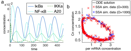
Figure 1: The dynamics of the exemplar systems. a. The (deterministic) solutions of the NF-$\kappa$B system responding to a continuous TNF$\alpha$ stimulation plotted against time. Here only 4 variables are presented, specifically the concentrations of the inhibitor protein I$\kappa$B$\alpha$ in the cytoplasm, the NF-$\kappa$B concentration in the nucleus, the concentration of the active kinase of the inhibitor IKKa, and of the A20 protein. Observe that the I$\kappa$B$\alpha$ is negatively correlated with NF-$\kappa$B , same with A20 and IKKa. b. The ODE solutions of the Drosophila circadian clock and simulated data produced using the SSA. Two variables are presented and plotted against each other. These are the mRNA expression levels of per gene, and the concentration of its inhibitor, $C_{n}$, which is a a complex formed by a (phosphorylated) form of proteins Per and Tim.

2 Reaction network dynamics and the pcLNA model

We consider a system of multiple populations, $M_{1},M_{2},\dots,M_{n}$, that interact between each other according to a fixed number of $R$ interactions, in this context called reactions. These populations might be for instance the Susceptible, Infected and Recovered individuals in epidemiology, the predators and prey in ecology, or various molecular populations in biochemistry. Reactions can be described by

$$k_{1j}M_{1}+\dots+k_{nj}M_{n}\stackrel{{\scriptstyle c_{j}}}{{\longrightarrow}}k_{1j}^{\prime}M_{1}+\dots+k_{nj}^{\prime}M_{n},\qquad k_{lj},k_{lj}^{\prime}\geq 0,\;l=1,\dots,n$$

where on the left hand side, $k_{lj}$ gives the number of individuals of population $M_{l}$ that is needed for the reaction to happen and on the right hand side, $k^{\prime}_{lj}$ gives the number of $M_{l}$ individuals that is produced by the reaction, where $l=1,\dots,n$ and $j=1,\dots,R$. The populations $M_{l}$ with $k_{lj}\neq 0$ are called reactants while those with $k^{\prime}_{lj}\neq 0$ are called products of the reaction. The vector ${\bm{a}}_{j}=(k_{1j}-k_{1j}^{\prime},\dots,k_{nj}-k_{nj}^{\prime})^{T}$ describes the net change after one occurrence of the $j$-th reaction. We call the matrix ${\bm{A}}$ with columns ${\bm{a}}_{j}$, $j=1,\dots,R$, the stoichiometry matrix of the reaction network. The positive constant $c_{j}$ indicates the frequency of the reaction.

We define the state ${\bm{x}}(t)=(x_{1}(t),\dots,x_{n}(t))^{T}$ where the $l$-th entry gives the number of individuals of the $M_{l}$ population at time $t\geq 0$. Under the assumption that the populations live in a well-mixed environment with constant conditions (see Gillespie (1992)), the occurrence of the next reaction of type $j$ follows an exponential distribution. The rate of this exponential distribution depends on the state of the reactants and the constant $c_{j}$. If the current state ${\bm{x}}(t)={\bm{x}}$, then a general form of the rate of the $j$-th reaction is $w_{j}({\bm{x}})=c_{j}\prod_{l}{\bm{x}}_{l}^{k_{lj}},$ but it is worth noting that other forms (e.g. $w_{j}({\bm{x}})=c_{j}\frac{k}{k+x_{l}}$, $k>0$) are also commonly used. The parameters involved in the reactions (e.g. $c_{j}$, $k$) are typically unknown and we will attempt to estimate them in the following sections. The stochastic process describing the evolution of state ${\bm{x}}(t)$ in time $t\geq 0$ is a continuous time-inhomogeneous Poisson process, where the inhomogeneity is due to the non-constant, state-dependent rates. The evolution of the probability distribution of this Poisson process over time can be described by the so-called master equation, which is the Kolmogorov-Smirnov equation of this process (see Wilkinson (2011)). The master equation can only be solved very rarely, but an exact stochastic simulation called Stochastic Simulation Algorithm (SSA), also known as Gillespie algorithm (Gillespie, 2000), can be used to generate stochastic trajectories that exactly follow the probability distribution of the Poisson process. A number of approximate models and simulation algorithms have been developed (Gillespie and Petzold, 2003; Gillespie, 2000).

We next describe the standard Linear Noise Approximation (LNA) model (Van Kampen, 2007; Kurtz, 1970, 1971). The LNA gives the state of the system at time $t>0$ by

$${\bm{x}}(t)=\Omega\bm{\varphi}(t)+\sqrt{\Omega}\,\bm{\xi}_{t}.$$ (2.1)

The term $\Omega$ is a parameter, often called system size, that is typically considered as a known property of the system (e.g. cell volume, total population size). It is not necessary to identify such a parameter (i.e. it can be fixed to 1), but in some cases, in particular for the NF-$\kappa$B system that we consider, the parameter has been estimated for certain cell types.

Then $\bm{\varphi}_{t}=\bm{\varphi}(t;\bm{\theta})$ is a (deterministic) solution of the ODE

$$d\bm{\varphi}_{t}={\bm{F}}(\bm{\varphi}_{t}){dt},\quad{\color[rgb]{0,0,0}{\text{where }{\bm{F}}(\bm{\varphi}_{t})={\bm{A}}{\bm{r}}(\bm{\varphi}_{t})}}.$$ (2.2)

The vector ${\bm{r}}(\bm{\varphi}_{t})=(r_{1}(\bm{\varphi}_{t}),\dots,r_{R}(\bm{\varphi}_{t}))^{T}$ has entries the classical rates of each reaction that satisfy the macroscopic law of reactions (see Wilkinson (2011)). Each entry $r_{j}(\cdot)$ is related to the corresponding function $w_{j}(\cdot)$ typically by $w_{j}({\bm{x}})=\Omega r_{j}({\bm{x}}/\Omega)$. The solution $\bm{\varphi}_{t}$ is a macroscopic ($\Omega\to\infty$) limit of ${\bm{x}}(t)/\Omega$.

Finally $\bm{\xi}_{t}=\bm{\xi}(t)$ is the solution of the SDE

$$d\bm{\xi}_{t}=\bm{J}_{t}\bm{\xi}_{t}dt+{\bm{S}}_{t}^{1/2}d\bm{w}_{t}.$$ (2.3)

The drift matrix of the SDE in (2.3) is the Jacobian matrix of the system in (2.2), i.e. $\bm{J}_{t}=\bm{J}(\bm{\varphi}_{t})=(dF_{i}(\bm{\varphi}_{t})/d\varphi_{j})_{i,j}$, while ${\bm{S}}_{t}={\bm{A}}{\bm{R}}(\bm{\varphi}_{t}){\bm{A}}^{T}$ with ${\bm{R}}(\bm{\varphi})$ a diagonal matrix with main diagonal ${\bm{r}}(\bm{\varphi})$. The stochastic process $\{\bm{w}_{t}:t\geq 0\}$ is a classical $N$-dimensional Wiener process.

The key advantage of the LNA over other approximate models is that the SDE in (2.3) can be solved analytically with the solution satisfying

$$\bm{\xi}_{t}={\bm{C}}(t_{0},t)\bm{\xi}_{t_{0}}+{\bm{\eta}}_{t},\quad{\bm{\eta}}_{t}\sim N(0,{\bm{V}}(t_{0},t)).$$ (2.4)

Here the matrices ${\bm{C}}$ and ${\bm{V}}$ are solutions of the initial value problems,

$$d{\bm{C}}/dt =\bm{J}_{t}{\bm{C}}, {\bm{C}}(t_{0},t_{0})={\bm{I}},$$ (2.5)

$$\quad d{\bm{V}}/dt =\bm{J}_{t}{\bm{V}}+{\bm{V}}\bm{J}_{t}^{T}+{\bm{S}}_{t}, {\bm{V}}(t_{0},t_{0})={\bm{0}}$$ (2.6)

where ${\bm{I}}$ and ${\bm{0}}$ are the $n\times n$ identity and zero matrix, respectively.

Equation (2.4) implies that the transition probabilities $P(\bm{\xi}(t_{1})|\bm{\xi}(t_{0})=\bm{\xi}_{0})$ and $P({\bm{x}}(t_{1})|{\bm{x}}(t_{0})={\bm{x}}_{0})$, where $\bm{\xi}_{0}$ and ${\bm{x}}_{0}$ fixed values, are MVN, for any $t_{1}>t_{0}$, and also more generally that, if the initial condition $\bm{\xi}(t_{0})$ is a random vector with MVN distribution, the transition probabilities of the LNA model $P({\bm{x}}(t_{1})|{\bm{x}}(t_{0}))$ are also MVN. We can also show that the joint probability distribution of time series $({\bm{x}}(t_{0}),{\bm{x}}(t_{1}),\dots,{\bm{x}}(t_{n}))$ are multivariate normal with precision matrix that has a block tridiagonal form. Practically, using the LNA involves solving the ODE system in (2.2) for appropriate initial conditions, and then using this solution $\bm{\varphi}(t)$ to compute the matrices $\bm{J}=\bm{J}(\bm{\varphi}(t))$ and ${\bm{S}}={\bm{S}}(\bm{\varphi}(t))$, and solve (2.5), and (2.6). The solutions $\bm{\varphi}(t)$, ${\bm{C}}(t,t_{0})$, ${\bm{V}}(t,t_{0})$, $t\in[t_{0},T]$ can be used for deriving the probability distribution of the state of the system, performing simulations, computing the FIM of the model parameters, statistical inference (see below), and other purposes.

The accuracy of the standard LNA model depends on the system dynamics, and the relation between $\Omega$ and $T-t_{0}$, i.e. the length of the time-interval to be described. For instance, the LNA model is shown to be accurate for long-times when describing the dynamics of a stochastic dynamical system that has reached the neighborhood of an equilibrium of the system in (2.2). An accurate LNA can also be derived for any system when for a given $\Omega$, the length of the time-interval is chosen to be sufficiently short (see Grima et al. (2011), Wallace et al. (2012)). However, it is inaccurate in describing the long-time behaviour of stochastic systems presenting oscillations. For instance, we found that the standard LNA model is inaccurate when describing the NF-$\kappa$B and circadian clock oscillations even for time-intervals less than one oscillation cycle (Minas and Rand (2017)).

By studying the dynamics of oscillatory systems that present attractive limit cycles, the phase corrected LNA model (pcLNA) takes advantage of the stability of these systems in all-but-one directions of the state space. That is, these systems are stable in the $N-1$ transversal directions to the limit cycle. This stability is reflected into the stochastic dynamics. More specifically, Minas and Rand (2017) compare the joint probability distributions of SSA trajectories at multiple transversal sections with the corresponding Multivariate Normal distributions derived analytically under the LNA model to show that they are approximately equal. The variation in the unstable tangental direction can be controlled by frequently correcting the phase of the system between standard LNA transitions. The frequency depends on the dynamics of the system and the scale of stochasticity (here expressed by parameter $\Omega$). Minas and Rand (2017) observed that about 3-4 corrections per oscillation cycle was sufficient for the NF-$\kappa$B system and the Drosophila circadian clock model ($\Omega\in(300,2000)$).

For a system with limit cycle solution, $\bm{\varphi}(t)$, $t\in[0,\pi]$, with period $\pi$, the pcLNA model at times $t_{1},\dots,t_{N}$ is described by the following equations

(State) $${\bm{x}}_{i}={\bm{x}}(t_{i})=\Omega\bm{\varphi}_{i}\!+\!\sqrt{\Omega}\,\bm{\xi}_{i},$$ (2.7)

(Transition) $$\bm{\varphi}_{i}=\bm{\varphi}(s_{i-1}\!+\!\Delta t_{i}), \Delta t_{i}=t_{i}-t_{i-1}\qquad$$ (2.8)

$$\bm{\xi}_{i}={\bm{C}}(s_{i-1},s_{i-1}\!+\!\Delta t_{i})\,\bm{\kappa}_{i-1}+{\bm{\eta}}_{i}, {\bm{\eta}}_{i}\sim N(0,{\bm{V}}(s_{i-1},s_{i-1}\!+\!\Delta t_{i})),\;\qquad$$ (2.9)

(Phase correction) $$s_{i-1}\!=\!\operatorname*{arg\,min}\limits_{s\in[0,\pi]}d\left(\frac{{\bm{x}}_{i-1}}{\Omega},\bm{\varphi}(s)\right), \bm{\kappa}_{i-1}=({\bm{x}}_{i-1}-\Omega\bm{\varphi}_{i-1})/\sqrt{\Omega}$$ (2.10)

The only difference between pcLNA and the standard LNA model is the phase correction step in equation (2.10). There we find the phase-time, $s_{i-1}$, such that the point, $\bm{\varphi}(s_{i-1})$, which is on the limit cycle, minimises the distance $d({\bm{x}}_{i-1},\bm{\varphi}(s))$ to the state ${\bm{x}}_{i-1}$. If $d$ is the Euclidean distance metric, then $\bm{\varphi}(s_{i-1})$ is the point on the limit cycle that is the closest to the state ${\bm{x}}(t_{i-1})$. It is also the intersection point of the limit cycle and the orthogonal transversal section at $\bm{\varphi}(s_{i-1})$. The stochastic term is next adjusted to $\bm{\kappa}_{i-1}$ that lies on the transversal section, and is orthogonal to the tangential direction, which implies the elimination of noise in the unstable tangential direction. The search for the minimum distance in equation (2.10) can be performed by an optimization method (we use the standard Newton-Raphson method), and it is extremely fast, partly due to the search in the constraint space $[0,\pi]$. Note that a single set of solutions of the initial value problems in eqs. 2.2, 2.5 and 2.6 of the LNA are used for computing the states at all time-points, which makes simulations extremely fast.

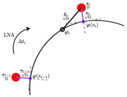
Figure 2: The pcLNA transitions. The phase corrected states of the underlying deterministic and stochastic process $\bm{\varphi}_{t}$ and $\bm{\xi}_{t}$, respectively, are used to proceed using the standard LNA transition equations.

As discussed earlier, we found that 3-4 phase corrections per cycle are needed to achieve high accuracy. In experimental settings, multiple time-points per cycle will be observed in order to study the oscillations. If more than 4 time-points are obtained per cycle, one may omit the phase correction step for some time-points, i.e. perform standard LNA transitions for some time-points, which would speed up the computation slightly without seriously affecting accuracy.

3 The pcLNA Kalman Filter

We now consider time-series observations of the system ${\bm{y}}=({\bm{y}}_{0},{\bm{y}}_{1},\dots,{\bm{y}}_{N})$ where ${\bm{y}}_{i}={\bm{y}}(t_{i})$ and $0\leq t_{0}\leq\dots\leq t_{N}$. We assume that the observation ${\bm{y}}_{i}=({\bm{y}}_{1i},\dots,{\bm{y}}_{qi})$ is related to the state ${\bm{x}}_{i}={\bm{x}}(t_{i})$ by

$${\bm{y}}_{i}={\bm{y}}(t_{i})={\bm{B}}{\bm{x}}_{i}+\bm{\epsilon}_{i}.$$ (3.1)

Here the matrix ${\bm{B}}$ in the observation equation (3.1) is a constant $q\times n$ matrix that determines how the observation relates to the underlying stochastic process. For example, ${\bm{B}}$ might eliminate unobserved variables in ${\bm{x}}$. The $m$-dim vectors $\bm{\epsilon}_{i}$, $i=1,\dots,N$ are independent (between them and to ${\bm{x}}$) measurement errors with normal distribution $N(0,\bm{\Sigma}_{e})$.

We derive a Kalman Filter to compute the likelihood

$$L(\bm{\theta};{\bm{y}})=\prod_{i=0}^{N}P({\bm{y}}_{i}|{\bm{y}}_{(i-1)};\bm{\theta}),\quad{\bm{y}}_{(i-1)}=({\bm{y}}_{0},\dots,{\bm{y}}_{i-1})$$ (3.2)

of the model parameters $\bm{\theta}$. Here we denote by ${\bm{y}}_{(-1)}=(\bm{\mu}_{0},\bm{\Sigma}_{0})$, where $\bm{\mu}_{0}$, and $\bm{\Sigma}_{0}$ the prior mean and variance of the state ${\bm{x}}$The Kalman Filter is a recursive algorithm (see Grewal and Andrews (2014)) that uses the model’s transition equations and Bayes rule to repeatedly perform the transition from prior to posterior distributions to obtain the likelihood factors $P({\bm{y}}_{i}|{\bm{y}}_{(i-1)};\bm{\theta})$, for $i=1,2,\dots,N-1$.

The pcLNA Kalman Filter transitions are governed by the observation equation in (3.1) and the pcLNA equations (2.7)-(2.10).

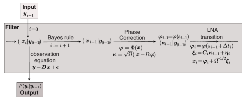
Figure 3: The iterative steps of the pcLNA Kalman filter. The filter starts by taking the inputs ${\bm{y}}_{i-1}$ and goes through a cycle of applying the Bayes rule, phase correction, and LNA transition to derive $({\bm{x}}_{i}|{\bm{y}}_{(i-1)})$. Each time the filter reaches the latter step, it applies the observation equation to output a likelihood factor.

We now outline the steps of the pcLNA Kalman Filter algorithm. We use the notation $P_{N}(\cdot\,|{\bm{m}},{\bm{S}})$ to denote the pdf of a MVN distribution with mean vector ${\bm{m}}$ and variance matrix ${\bm{S}}$. The mean and variance of observation ${\bm{y}}_{i}$ are denoted by $\{\bm{\mu}^{({\bm{y}})}_{i},\bm{\Sigma}^{({\bm{y}})}_{i}\}$, prior means and variances of $({\bm{x}}_{i}|{\bm{y}}_{(i-1)})$ and $(\bm{\kappa}_{i}|{\bm{y}}_{(i-1)})$ by $\{\bm{\mu}_{i},\bm{\Sigma}_{i}\}$ and $\{{\bm{m}}_{i},{\bm{S}}_{i}\}$, with the symbol ^∗ denoting the corresponding posterior parameters.

1. Input $\left({\bm{y}}_{-1},{\bm{y}}_{0},{\bm{y}}_{1},\dots,{\bm{y}}_{N}\right)$, $\bm{\varphi}$, ${\bm{C}}$, ${\bm{V}}$, ${\bm{B}}$ and $\bm{\Sigma}_{e}$.
   

2. Compute $\bm{\mu}^{({\bm{y}})}_{0}={\bm{B}}\bm{\mu}_{0}$, $\bm{\Sigma}^{({\bm{y}})}_{0}=\bm{\Sigma}_{0}+\bm{\Sigma}_{e}$. Output: $P({\bm{y}}_{0};\bm{\theta})=P_{N}({\bm{y}}_{0}|\bm{\mu}^{({\bm{y}})}_{0},\bm{\Sigma}^{({\bm{y}})}_{0})$.
   

3. For iteration $i=1,2,\ldots,N-1$

   1. Compute the posterior mean and variance of $({\bm{x}}_{i-1}|{\bm{y}}_{(i-1)})$

      $$\bm{\mu}^{*}_{i-1} = \bm{\mu}_{i-1}+\bm{\Sigma}_{i-1}{\bm{B}}^{T}(\bm{\Sigma}^{\bm{y}}_{i-1})^{-1}\hat{\bm{\epsilon}}_{i-1},\quad\hat{\bm{\epsilon}}_{i-1}={\bm{y}}_{i-1}-\bm{\mu}^{\bm{y}}_{i-1}$$

      $$\bm{\Sigma}^{*}_{i-1} = \bm{\Sigma}_{i-1}-\bm{\Sigma}_{i-1}{\bm{B}}^{T}(\bm{\Sigma}^{\bm{y}}_{i-1})^{-1}{\bm{B}}\bm{\Sigma}_{i-1}$$

   2. Compute $\bm{\varphi}_{i-1}:=\bm{\varphi}(s_{i-1})=\operatorname*{arg\,min}_{s\in[0,\pi]}d(\bm{\mu}^{*}_{i-1},\bm{\varphi}(s))$ and the posterior mean and variance of $(\bm{\kappa}_{i-1}|{\bm{y}}_{(i-1)})$

      $${\bm{m}}^{*}_{i-1} = \Omega^{1/2}(\bm{\mu}^{*}_{i-1}-\bm{\varphi}_{i-1})$$

      $${\bm{S}}^{*}_{i-1} = \Omega{\bm{E}}_{2}\left(\bm{\Sigma}_{22,i-1}^{*}-\frac{(\bm{\Sigma}_{12,i-1}^{*})^{T}\bm{\Sigma}_{12,i-1}^{*}}{\bm{\Sigma}_{11,i-1}^{*}}\right){\bm{E}}_{2}^{T}$$

      where ${\bm{E}}_{2}:=[{\bm{e}}_{2}\cdots{\bm{e}}_{n}]$ with ${\bm{e}}_{j}^{T}{\bm{e}}_{j^{\prime}}=0$, $j,j^{\prime}\in\{1,2,\dots,n\}$, and ${\bm{e}}_{1}:={\bm{F}}(\bm{\varphi}_{i-1})$. Here

      $$\bm{\Sigma}^{*}_{11,i-1}=e_{1}^{T}\bm{\Sigma}^{*}_{i-1}e_{1},\quad\bm{\Sigma}^{*}_{12,i-1}=e_{1}^{T}\bm{\Sigma}^{*}_{i-1}E_{2},\quad\bm{\Sigma}^{*}_{22,i-1}=E_{2}^{T}\bm{\Sigma}^{*}(t)E_{2}.$$

   3. Compute the prior mean and variance matrix of $({\bm{x}}_{i}|{\bm{y}}_{(i-1)})$

      $$\bm{\mu}_{i} = \bm{\varphi}_{i}+{\bm{C}}(s_{i-1},s_{i}){\bm{m}}^{*}_{i-1},\,\bm{\varphi}_{i}=\bm{\varphi}(s_{i}),\,s_{i}=s_{i-1}+\Delta t_{i},\,\Delta t_{i}=t_{i}-t_{i-1}$$

      $$\bm{\Sigma}_{i} = {\bm{C}}(s_{i-1},s_{i}){\bm{S}}^{*}_{i-1}{\bm{C}}(s_{i-1},s_{i})^{T}+{\bm{V}}(s_{i-1},s_{i})$$

   4. Compute $\bm{\mu}^{{\bm{y}}}_{i}={\bm{B}}\bm{\mu}_{i}$, $\bm{\Sigma}^{\bm{y}}_{i}=\bm{\Sigma}_{i}+\bm{\Sigma}_{e}$.
      Output: $P({\bm{y}}_{i}|{\bm{y}}_{(i-1)};\bm{\theta})=P_{N}({\bm{y}}_{i}|\bm{\mu}^{{\bm{y}}}_{i},\bm{\Sigma}^{\bm{y}}_{i})$.

As we illustrate in Figure 3, in steps (KF2) and (KF3)(KF3d) we used the observation equation to derive the likelihood terms. In step (KF3)(KF3a), we used Bayes rule to derive the posterior distribution, and in steps (KF3)(KF3c) the transition equations. In step (KF3)(KF3b), the phase correction in (2.10) is performed using the Euclidean distance, which implies that the transversal sections are orthogonal to the tangent vectors ${\bm{F}}(\varphi)$ in $\eqref{eq:ode}$. A Newton-Raphson algorithm is used to find the point $\bm{\varphi}(s_{i-1})$ as in (2.10). The posterior distributions $(\bm{\kappa}_{i-1}|{\bm{y}}_{(i-1)})$ are then projections (on the orthogonal transversal section) of the conditional distribution of the noise $(\bm{\xi}_{i-1}|{\bm{y}}_{(i-1)})$, with $\bm{\xi}_{i-1}$ as in $\eqref{eq:stTr}$.

3.0.1 Multiple time-series

Typically data consist of multiple independent time-series of observations, possibly with observations taken at different time-points. In this case, the joint likelihood of the multiple time-series is simply the product of the likelihood of each time-series that can be computed based on the above Kalman Filter. If the same initial condition is used for all time-series, then the LNA system in eqs. 2.2, 2.5 and 2.6 needs to be solved only once for all time-series. This assumption might be suitable when the experimental design implies that the oscillating system is initialised in the same experimental conditions. For instance, for the NF-$\kappa$B system that we consider, each time-series correspond to different cells. These cells at the initial time-point are left at resting state for an appropriate time interval before applying an activating signal. The noise around the initial condition is incorporated into the model by the distribution of $\bm{\xi}_{0}$. Therefore, the use of the same initial conditions is not only appropriate but also preferable because it allows us to draw inference for them from the data. Alternatively, the initial conditions might differ only by their phase in the oscillating cycle. Again the LNA system can be solved once and the phase of the system at the initial time-point can be identified by phase correction.

Finally, if the initial conditions differ vastly one might wish to use a different initial condition for each time-series with additional computational cost.

4 System sensitivity analysis and identifiability

Due to the coupling between the variables of non-linear dynamical systems in biology, it is frequently the case that parameters are fully or partially non-identifiable. Local sensitivity metrics such as Fisher information enable a study of parameter identifiability in the system and can therefore provide an a priori indication of which parameter(s) are identifiable. Here, we will show how a decomposition of the Fisher Information matrix allows us to define parameter sensitivity coefficients that capture the effect of changes in parameter values on the likelihood.

Fisher Information quantifies the information that an observable random variable carries about an unknown parameter $\theta$. If $P_{\bm{\theta}}({\bm{x}})$ is the probability density function of a continuous random vector ${\bm{x}}$ depending on parameter vector $\bm{\theta}$, the Fisher Information Matrix (FIM) $\mathcal{I}=\mathcal{I}_{\bm{\theta}}$ has entries

$$\mathcal{I}_{ij}=E\left[\frac{\partial\ell}{\partial\theta_{i}}\frac{\partial\ell}{\partial\theta_{j}}\right]=-E\left[\frac{\partial^{2}\ell(\theta;{\bm{x}})}{\partial\theta_{i}\partial\theta_{j}}\right],$$ (4.1)

where $\ell=\log P_{\bm{\theta}}$, and $\theta_{i}$ and $\theta_{j}$ are the $i$th and $j$th components of the parameter vector $\bm{\theta}$. If $P_{\bm{\theta}}$ is Multivariate Normal (MVN) with mean vector $\bm{\mu}=\bm{\mu}(\bm{\theta})$ and covariance matrix $\bm{\Sigma}=\bm{\Sigma}(\bm{\theta})$ then

$$\mathcal{I}_{ij}=\frac{\partial\bm{\mu}}{\partial\theta_{i}}^{T}\bm{\Sigma}^{-1}\frac{\partial\bm{\mu}}{\partial\theta_{j}}+\frac{1}{2}\text{tr}\left(\bm{\Sigma}^{-1}\frac{\partial\bm{\Sigma}}{\partial\theta_{i}}\bm{\Sigma}^{-1}\frac{\partial\bm{\Sigma}}{\partial\theta_{j}}\right).$$ (4.2)

The FIM measures the sensitivity of $P_{\bm{\theta}}$ to a change in parameters in the sense that

$$D_{KL}(P_{\bm{\theta}+\delta\bm{\theta}}||P_{\bm{\theta}})=\frac{1}{2}\delta\bm{\theta}^{T}\mathcal{I}_{\bm{\theta}}\delta\bm{\theta}+\text{O}(||\delta\bm{\theta}||^{3})$$

where $D_{KL}$ is the Kullback-Leibler divergence between the distribution of the random vector ${\bm{x}}$ with parameter $\bm{\theta}$ and the distribution of ${\bm{x}}$ with parameter $\bm{\theta}+\delta\bm{\theta}$. The significance of the FIM in (4.1) for sensitivity and experimental design follows from its role as an approximation to the Hessian of the log-likelihood function at a maximum. Assuming non-degeneracy, the likelihood of a parameter value $\bm{\theta}$ near the maximum likelihood estimate $\bm{\theta}^{*}$ is

$$\ell(\bm{\theta})\approx\ell(\bm{\theta}^{*})-\frac{1}{2}\sum_{i}\sigma_{i}^{2}\left.\bm{\theta}^{\prime}_{i}\right.^{2},$$

where $\sigma_{i}^{2}$ are the eigenvalues ($\sigma_{i}$ the singular values), and $\bm{\theta}^{\prime}_{i}$ the coordinates of the parameter $\bm{\theta}$ with respect to an eigenbasis of the FIM in (4.1) If we assume that the $\sigma_{i}$ are ordered so that $\sigma_{1}^{2}\geq\cdots\geq\sigma_{s}^{2}$ then it follows that near the maximum the likelihood is most sensitive when $\theta^{\prime}_{1}$ is varied and least sensitive when $\theta^{\prime}_{s}$ is. Moreover, $\sigma_{i}$ is a measure of this sensitivity.

Furthermore, because the FIM $\mathcal{I}_{\bm{\theta}}$ is symmetric and positive semi-definite, it can be decomposed to $\mathcal{I}=\underline{{\bm{s}}}^{T}\underline{{\bm{s}}}$and the KL divergence

$$D_{\text{KL}}(P_{{\bm{\theta}}+\delta{\bm{\theta}}}||P_{{\bm{\theta}}})=\frac{1}{2}\|\underline{{\bm{s}}}\,\delta{\bm{\theta}}\|^{2}+\text{O}(||\delta{\bm{\theta}}||^{3})=\frac{1}{2}\sum_{i,j,l}\delta\theta_{j}\delta\theta_{l}\underline{{\bm{s}}}_{ij}\underline{{\bm{s}}}_{il}+\text{O}(||\delta{\bm{\theta}}||^{3}).$$ (4.3)

The length, $\|\,\underline{{\bm{s}}}_{j}\,\|^{2}=2D_{\text{KL}}(P_{{\bm{\theta}}+\delta\bm{e}_{j}}||P_{{\bm{\theta}}})+\text{O}(||\delta{\bm{\theta}}||^{3})$, of the $j$-th column vector $\underline{{\bm{s}}}_{j}=(\underline{{\bm{s}}}_{1j},\dots,\underline{{\bm{s}}}_{kj})^{T}$ of $\underline{{\bm{s}}}$, measures the effects of a single unit change of the $j$-th parameter $\theta_{j}$ to the distribution $P_{\bm{\theta}}$, $j=1,\dots,k$, i.e. $D_{\text{KL}}(P_{{\bm{\theta}}+\delta\bm{e}_{j}}||P_{{\bm{\theta}}})=\frac{1}{2}\delta^{2}\|\underline{{\bm{s}}}_{j}\|^{2}+\text{O}(|\delta|^{3})$, where $\bm{e}_{j}$ the unit vector with only non-zero entry being the $j$-th entry. It can therefore be used to study the sensitivity of $P$ to changes in the parameter values.

4.1 Computation of FIM for reaction network dynamics

The computation of the Fisher Information matrix requires the computation of the derivatives of the likelihood in (4.1). If the data distribution is assumed to be Multivariate Normal then this computation reduces to computing derivatives of the mean vector and covariance matrix. In the case where observations are time-series with assumed model the continuous time-inhomogeneous Poisson process of reaction network dynamics, the computation of likelihood and even more the derivatives required for the FIM are very rarely computationally feasible. The LNA model gives Multivariate Normal distributions for time-series observations and FIM computation is feasible, but it is often inaccurate for oscillatory dynamics as we explained in section 2. The pcLNA model requires a Kalman Filter to compute the likelihood of time-series observations as a product of transition densities that are Multivariate Normal. It is possible but computationally intensive to compute the required derivatives of these likelihood functions. Here we opt for computing the FIM with the likelihood function set as the joint probability distribution, derived in Minas and Rand (2017) (see Supplementary information 1, section 9 for details), of trajectories transitioning between a large number of transversal sections of the limit cycle solutions of the studied systems under the LNA model. We ask whether the sensitivity coefficients of this FIM can predict which parameters are identifiable. Note that we use the pcLNA Kalman Filter described in section (3) to compute the likelihood of time-series observations. Both these likelihood functions are derived under the LNA model and they both control the instability of oscillatory dynamics in the tangential direction, only in a different way as explained in section 2. In section 6, we will try to answer this question by applying our methodology to our exemplar systems and comparing the outputs with our sensitivity analysis predictions.

5 Markov chain Monte Carlo algorithms

We implement a Bayesian analysis to conduct inference on the selected parameters within the model systems. Previous analyses of smaller systems (e.g. Girolami and Calderhead, 2011; Burton et al., 2021) have shown that the choice of inference algorithm can severely impact the efficiency of the parameter estimation for even relatively small dynamical systems. The likelihood of time-series observations is derived through the Kalman Filter and has the form of a product of conditional Multivariate Normal densities as explained above. It’s not possible to derive the full conditional distributions for the parameters due to the complex dependence of the likelihood to the parameters and therefore we cannot utilise Gibbs samplers to conduct inference.

Due to the nature of the dynamics of the systems, previous studies have found significant problems of poor mixing in chains when conducting analyses on small stochastic systems (e.g. Fearnhead et al., 2014).

To overcome these challenges, we implement three different Monte Carlo algorithms, namely a parallel-tempered Random Walk algorithm (Gupta et al., 2018) and a simplified manifold Metropolis adjusted Langevin algorithm (Girolami and Calderhead, 2011), with a random walk Metropolis algorithm. We do not formally compare the three algorithms, but show how each can be used in models of this kind and some of the challenges that are common to these stochastic complex systems.

5.0.1 Random Walk Metropolis algorithm

The first baseline approach used a random walk Metropolis algorithm, with proposal distribution $q(.)$ set as a multivariate Normal distribution centered on the current parameter vector $\mathbf{\theta^{t}}$ and with diagonal covariance matrix $\mathbf{\Sigma=\mathbf{\sigma^{2}I}}$. The proposal variances were specified on the same order of magnitude as the simulated parameter value. Multivariate new parameter values $\mathbf{\theta^{t+1}}$ are subsequently drawn from the proposal distribution, and are accepted jointly with probability $\alpha(\mathbf{\theta^{t},\theta^{t+1}})$. More complex covariance proposals were also considered, using pilot runs, however these were not found to work well due to the complex behaviour of the systems around specific parameter values.

Due to the general properties of MH algorithms to get stuck in local modes, especially in high-dimensional problems or multimodal densities, alternative algorithms were also tested.

5.0.2 Simplified Manifold MALA

Girolami and Calderhead (2011) propose geometric MCMC algorithms, that use a metric tensor $\mathbf{G(\theta)}$ specified on the target posterior distribution to move efficiently around parameter space. Using the local geometric structure of the target around the current parameter value, proposed moves are made along a manifold in the multivariate space to move more swiftly towards regions of high posterior probability. Multiple variants of traditional MCMC methods are proposed, however the approach used here is a manifold algorithm using an approximation to the Fisher information matrix as the metric tensor $\mathbf{G(\theta)}$, based on the mean component of the Kalman-Filter likelihood.

The proposal distribution utilised, $q(\mathbf{\theta})$, is then

$$N\left(\mathbf{\theta}+\frac{\epsilon^{2}}{2}\mathbf{G^{-1}(\theta)}\nabla_{\theta}\mathcal{L}\{\mathbf{\theta}_{t}\},\;\epsilon^{2}\mathbf{G^{-1}(\theta)}\right)$$

where $\epsilon$ is tuned to provide reasonable acceptance rates.

Taking account of the higher order geometric structure of the posterior within the proposal has shown considerable improvements in effective sample size, albeit at a significant computational cost of calculating the system derivatives (Girolami and Calderhead, 2011). We test the simplified manifold MALA as a trade-off between computational efficiency and speed as it only requires the first-order partial derivatives of the likelihoods to be calculated.

5.0.3 Parallel tempering

A feasible solution to attempt to circumvent the problem of local modes is trying to run a population of Markov chains in parallel, each with possibly different, but related stationary distributions. Information exchange between distinct chains enables the target chains to learn from past samples, improving the convergence to the target chain (Gupta et al., 2018).

Parallel tempering (PT) is an algorithm that attempts periodic swaps between multiple Markov chains running in parallel at different temperatures, where samplers with shallower energy landscape can traverse between multiple modes more efficiently. Each chain is equipped with an invariant distribution connected to an auxiliary variable, the temperature $\beta$, which scales the shallowness of the energy landscape, and hence defines the probability of accepting an unsuitable move (Gupta et al., 2018; Hansmann, 1997). An increase in the temperature eases the traversal of the sample space. High temperature chains accept unfavourable moves with higher probability. As a result, higher temperature chains allow circumvention of local minima, improving both convergence and sampling efficiency (Chib and Greenberg, 1995).

Defining the energy $E[\theta^{*}]$ as the negative log-posterior evaluated at that parameter value, the Parallel Tempering algorithm for a parameter vector $\theta$ can be illustrated as follows.

• For $s=1,...,S$ swap attempts

  1. For $j=1,...,J$ chains

     1. For $t=1,...,N_{iter}$ iterations

        1. Propose a new parameter vector $\theta^{*}(j)$ from a symmetric distribution $q(\theta^{*}(j)|\theta(j))$

        2. Calculate the energy $E_{j}=E[\theta^{*}(j)]$

        3. Set $\theta_{t+1}(j)=\theta^{*}(j)$ with probability $min(1,e^{-\beta_{j}\Delta E_{j}})$, where $\Delta E_{j}=E[\theta^{*}(j)]-E[\theta_{t-1}(j)].$ Otherwise, set $\theta_{t+1}(j)=\theta_{t}(j)$.

     2. Record the value of the parameters and the energy on the final iteration

  2. For each consecutive pair of chains (in decreasing order of temperature)

     • Accept swaps with probability $min(1,e^{\Delta\beta\Delta E})$, where $\Delta E=E_{j}-E_{j-1}$ and $\Delta\beta=\beta_{j}-\beta_{j-1}.$

If $\beta_{c}=1$, then the exact posterior distribution of interest is being sampled, hence, samples of the chain where $\beta_{c}=1$ are retained and summary statistics calculated, with other chains used for improving convergence and subsequently discarded. An additional step could combine use an importance sampling approach to combine the chains, thus improving efficiency Gramacy et al. (2010).

6 Simulation studies

6.1 System analysis and identifiability

System sensitivity analyses were performed for the two exemplar systems using Fisher Information around the values of parameters reported in the literature as broadly representing the system dynamics. The analyses, which are shown in Figure 4, examine both the absolute and relative sensitivity of the model through the eigenvalues of the FIM, but also the model sensitivity to changes in the values of each parameter.

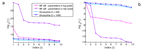
Figure 4: Eigenvalues of the FIM for the pcLNA model of the two exemplar systems. Plot (a) compares the 10 largest singular values of the FIM of: the NF-$\kappa$B system with model parameters in log- and raw-scale, the Drosophila circadian clock model for two values of the system size $\Omega$ (see legend). Plot (b) compares the 10 largest normalised (divided by the largest singular value) singular values of the FIM of the same models as in (a) (see legend). The NF-$\kappa$B system overall has larger sensitivities, but the FIM is dominated by few eigen-directions, while the clock model is more balanced in parameter sensitivities.

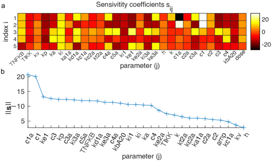
Figure 5: Sensitivity coefficients for the pcLNA model of the NF-$\kappa$B system with parameters in raw scale. Plot (a) is the heatmap of the sensitivity coefficients (in log scale, with base 2), $s_{ij}$, with $i=1,\dots,5$ as in (4.3) and plot (b) gives the overall sensitivity coefficient, $\|s_{j}\|$, of each parameter (j).

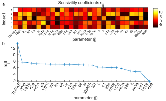
Figure 6: Sensitivity coefficients for the pcLNA model of the NF-$\kappa$B system with parameters in log scale. Plot (a) is the heatmap of the sensitivity coefficients (in log scale, with base 2), $s_{ij}$, with $i=1,\dots,5$ as in (4.3) and plot (b) gives the overall sensitivity coefficient, $\|s_{j}\|$, of each parameter (j) (in log-scale).

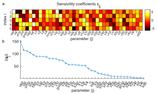
Figure 7: Sensitivity coefficients for the pcLNA model of the NF-$\kappa$B system with parameters in log scale. Plot (a) is the heatmap of the sensitivity coefficients (in log scale, with base 2), $s_{ij}$, with $i=1,\dots,5$ as in (4.3) and plot (b) gives the overall sensitivity coefficient, $\|s_{j}\|$, of each parameter (j) (in raw-scale).

The singular values of the FIM of the NF-$\kappa$B system with parameter changes in the log-scale are substantially larger than all other systems indicating a generally higher sensitivity in this model (see Figure 4a). However, the relative sensitivity of the same system is worse than any other considered system as the first two singular values dominate the magnitude of the FIM (see Figure 4b). The circadian clock model for both values of $\Omega$ exhibits a slow decrease in the first ten singular values of the system, which is translated as relatively small differences in the sensitivity of the model in a much larger number of directions of the parameter space, compared to the NF-$\kappa$B system. This suggests that the circadian clock will provide better mixing of the MCMC chains since the changes in the likelihood over the parameter space are more smooth compared to the NF-$\kappa$B system. In contrast, the sharp decrease of the singular values of the NF-$\kappa$B system indicate that the likelihood is much more sensitive to changes in a small number of directions of the parameter space (one for the log-scale and two for the raw scale) compared to any other direction. When conducting inference, the choice of scale to conduct inference on will also change depending on this variation in sensitivity.

From the sensitivity analysis, it is apparent that the two parameters associated with the two largest singular values of the NF-$\kappa$B system in the raw scale were those corresponding to the mRNA synthesis rates for the variables I$\kappa$B$\alpha$ and A20, namely $c1$ and $c1a$ respectively. Notice the white and black color for those parameters in the heatmap in Figure 5a and the corresponding high values of the overall sensitivity $\|{\bm{s}}_{j}\|$ in Figure 5b.

Different parameters were highlighted as sensitive on the log-scale, with substantially higher sensitivity coefficients primarily for total NF-$\kappa$B concentration (TNFKB) compared to all other parameters (see Figure 6).

The slow decay in the eigenvalues of the Drosophila circadian clock is reflected also in the parameter sensitivity coefficients with a larger number of parameters having closer sensitivities compared to those in the NF-$\kappa$B model. In particular, the sensitivities coefficients suggest that more parameters could be estimable.

We used these sensitivity analyses to guide the choice of parameters to estimate within the Bayesian inferential framework. In particular, we highlight the differences between estimating parameters with high sensitivity coefficients compared to estimating those with low sensitivity coefficients.We see whether there is a clear dependence between the sensitivity coefficients and the precision of posterior distributions. We also consider scenarios where a mix up of parameters with high and low sensitivity and coefficients is estimated. Other parameters not included in the inference are fixed at the respective values from the literature.

6.2 Parameter estimates and identifiability

For each of the different settings, ten independent stochastic trajectories were generated using either the pcLNA simulation algorithm (Minas and Rand, 2017) or the full SSA, with parameters fixed at those from available literature (Ashall et al., 2009; Gonze et al., 2003). This is a modest sample size for typical experiments of those systems.

6.2.1 NF-$\kappa$B system

We first run the three Markov chain Monte Carlo (MCMC) described in section 5 to the NF-$\kappa$B system with parameters in raw-scale. We should note that it is generally preferable to run the sensitivity analysis and estimation in log-scale. This is because the raw-scale is affected by the measurements units used to set the parameter values. A change in the measurement units can largely influence the sensitivities. Unless the parameters need to be estimated to a specific measurement unit, it is preferable to use the log-scale. In this first example, we simply consider the raw-scale because it provides an informative illustration of applying our methods, which is different to results in the log-scale.

Each of the three Markov chain Monte Carlo algorithms were run with 20000 iterations, the first 10000 being discarded as burn-in. For the parallel tempering algorithm, $k=4$ parallel chains were run with $\beta_{k}\in\{1,0.75,0.5,0.25\}$. Prior distributions were specified on each of the rate parameters on the raw scale, whilst inference was conducted both on the raw scale and on the log scale with appropriate Jacobian term applied to the acceptance probabilities in the case of the latter. Alternatively, priors could be specified on the log-scale, removing the need for the Jacobian term. Relatively vague Gamma(1,10) priors were specified on rate parameters and inverse Gamma IG(0.001,0.001) for the error variance. Unless stated otherwise, we assume $B$ is an identity matrix, that is all species are measured at all time points.

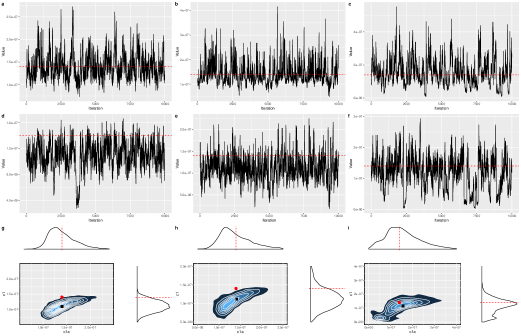
Figure 8: Posterior inference post-burn-in for parameters $c1a$ and $c1$ in the NF-$\kappa$B system, conducted on the original parameter scale. Top two rows show traceplots for parameter $c1a$ and $c1$ respectively with the bottom row showing bivariate marginal distributions. Each column relates to a single algorithm type (random walk Metropolis, SMMALA and parallel tempered random walk). Red dashed lines/circles correspond to the true parameter values and yellow circles the posterior mean.

Each of the three Markov chain Monte Carlo algorithms were initially run for the NF-$\kappa$B system with two unknown parameters ($c1a$ and $c1$) identified from the sensitivity analysis, with other parameters fixed at values from the literature. Posterior summary plots for the three algorithms are shown in 8. All three of these algorithms appeared to converge relatively quickly, and were centered on the true parameter values. Effective sample sizes were calculated for each of the three methods, with the geometric algorithm unsurprisingly showing on average a 35% improvement relative to the random walk Metropolis algorithm. The parallel tempering algorithm on average had a 52% reduction in ESS relative to the random walk algorithm. The main difference in posteriors between the three algorithms were observed in the parallel tempering algorithm, where a second mode close to zero was also occasionally visited by the the main chain. Although the initial chains look like they converged, clearly the smaller mode of the posterior was not visited by either of the two algorithms, hindered by the low-probability region between the two modes.

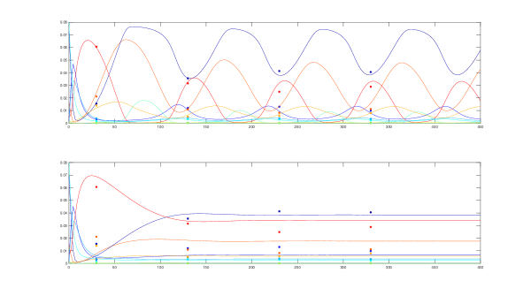
Figure 9: Deterministic solutions of the NF-$\kappa$B ODE system evaluated at the two posterior modes highlighted by the parallel tempering algorithm. The upper plot corresponds to a value close to the correct values, whilst the lower plot corresponds to values close to zero giving no oscillations beyond the first peak. The overlayed points correspond to the value of a randomly selected data sample. The colors represent the variables of the system.

Parameter	Algorithm	Truth	Post. mean	95% HPDI
$c1a$	RWM	1.4e-7	1.41e-7	9.28e-8	1.98e-7
	SMMALA		1.42e-7	7.45e-8	2.26e-7
	PT		1.57e-7	1.08e-8	3.08e-7
$c1$	RWM	1.4e-7	1.09e-7	7.15e-8	1.50e-7
	SMMALA		1.12e-7	5.76e-8	1.76e-7
	PT		1.16e-7	1.50e-8	2.05e-7

Table 1: Posterior summary statistics for the NF-$\kappa$B system on the raw scale. Data simulated from the pcLNA algorithm.

This second mode observed in the parallel tempering analysis was studied further to determine possible reasons that the tempered algorithm visited this mode and the biological implications of this. Figure 9 shows the deterministic solution to the system with parameters $c1a$ and $c1$ at the values from the literature and also again when replaced with the mean of this lower mode. This shows a clear problem with the discrete timepoints used for inference, as the observation times traditionally measured correspond only to the peaks of the nuclear NF-$\kappa$B. In this case, the algorithm correctly fails to reject parameters that give deterministic model solutions without oscillations as the level of nuclear NF-$\kappa$B remains constant at a similar level to the peak height in the oscillatory system. Biologically, this corresponds to a system with zero feedback between the corresponding variables.

As the parallel tempered algorithm was the only algorithm to effectively explore the multimodal parameter space, all further analyses were conducted using this algorithm. We further varied the parameter settings in the following ways.

6.2.2 Log-scale inference

The sensitivity analysis also showed variability depending on whether the parameters were transformed or not prior to conducting analysis. Whilst parameters $c1a$ and $c1$ were the most sensitive on the raw scale, when transforming parameters to a log scale, alternative parameters had higher sensitivity coefficients. We therefore also conducted inference on the log parameter scale using these parameters as the basis for inference. Despite this, there is one dominant singular value in the system so it was again expected this would correspond to the number of estimable parameter directions. Specifically, the total concentration of NF-$\kappa$B was the dominant parameter, with additional lower sensitivities to parameters (TNF$\alpha$) dose and $kbA20$. Additional parameters with much lower sensitivities, namely $kc1a$ and $c5a$, were included to test how these would behave in the inference. The total NF-$\kappa$B parameter determines the overall levels of all variables in the system. Prior distributions were kept similar to those in the previous analysis, specified on the un-transformed scale, but an appropriate Jacobian term was introduced into the Metropolis acceptance step to ensure the correct invariant distribution was reached. In the case of the log transform such that $\psi_{i}=\log(\theta_{i})$, with prior specified on the raw scale, the log posterior is $\log(\pi(\psi|\mathbf{y}))=\log(f(\mathbf{y}|\psi))+\sum_{i}\log(p(\exp(\psi_{i})))-\sum_{i}\log(\psi_{i})+constant$.

In each case, four chains were again run in parallel, with 20000 iterations consisting of 200 swaps in total, with swaps proposed every 100 iterations. The $\beta$ parameters across four chains were set at $\beta\in[1,0.5,0.2,0.1]$.

Parameter	Truth	Post. mean	95% HPDI
TNFKB	0.080	0.080	0.079	0.081
$kc1a$	0.074	0.115	0.072	0.186
$c5a$	2.2e-5	1.50e-4	1.77e-5	3.05e-4
$kbA20$	0.002	0.002	0.001	0.002
$dose$	1.000	1.026	0.890	1.240
$\sigma$	0.000	0.000	0.000	0.000

Table 2: Posterior estimates to 3d.p. for the NF$\kappa$B system with parameter inference conducted on the log-scale and all 11 variables measured. Data simulated from the pcLNA algorithm.

Table 2 presents posterior summaries of the results, in which the parameters can be reliably estimated. Posterior means were very close to the true parameter values, with all 95% HPDIs containing the true value for all parameters.

6.2.3 Unobserved variables

Further analyses were run under the setting that measurements of some of the biological species are not easily obtained experimentally. In this case, the matrix $\mathbf{B}$ in the Kalman filter is no longer an identity matrix, but contains some zero elements along the diagonal also. Table 3 shows the results for the same set-up as Table 2 but assuming only nuclear and cytoplasmic NF-$\kappa$B, cytoplasmic I$\kappa$B$\alpha$ and A20 are measurable.

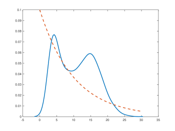
Figure 10: Prior distribution (dashed line) vs posterior marginal density (solid line) for the dose parameter when only four measurements are used.

The parallel tempered algorithm converged similarly in this case, but the ability to estimate some of the parameters deteriorated. Specifically, the dose parameter posterior distribution was very similar to the prior distribution, suggesting the data is non longer informative on this parameter (Figure 10) and the estimate of parameter $kc1a$ was positively biased towards the prior mean. The other parameters did not appear to be greatly impacted by the reduced measurement matrix. As the sensitivity coefficients are a sum over the sensitivities across all state variables in the system, if the dominant variable showing sensitivity to a given parameter is no longer measured, then the ability to practically identify that parameter will be removed. The number of dominant principal directions may also change.

Parameter	Truth	Post. mean	95% HPDI
$TNFKB$	0.080	0.079	0.066	0.092
$kc1a$	0.074	1.191	0.006	2.218
$c5a$	2.2e-5	3.69e-4	9.88e-5	6.79e-4
$kbA20$	0.002	0.007	0.001	0.016
$dose$	1.000	10.623	2.845	19.595
$\sigma$	0.000	0.000	0.000	0.000

Table 3: Posterior estimates for the NF$\kappa$B system with parameter inference conducted on the log-scale and only four variables measured. Data simulated from the pcLNA algorithm.

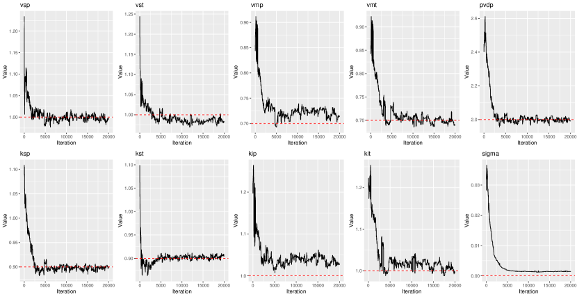
Figure 11: Posterior inference for the Drosophila circadian clock system estimating 9 parameters. Dashed horizontal line corresponds to the true parameter value used to simulate the data using the SSA.

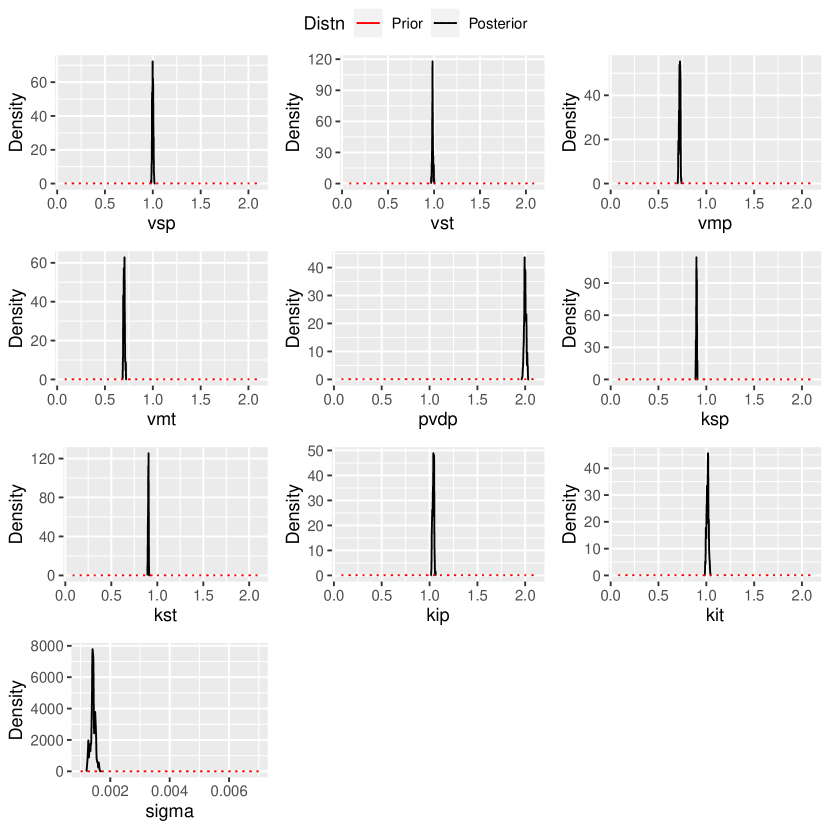
Figure 12: Drosophila marginal posterior densities (solid black) with corresponding prior density (dotted red).

Parameter	Truth	Post. mean	95% HPDI
$vsp$	1.000	0.999	0.987	1.009
$vst$	1.000	0.984	0.975	0.998
$vmp$	0.700	0.722	0.707	0.732
$vmt$	0.700	0.700	0.687	0.713
$pvdp$	2.000	1.999	1.976	2.021
$ksp$	0.900	0.898	0.890	0.906
$kst$	0.900	0.903	0.896	0.909
$kip$	1.000	1.038	1.023	1.052
$kit$	1.000	1.013	0.994	1.035
$\sigma$	0.000	0.001	0.001	0.002

Table 4: Posterior summary statistics for the estimated parameters in the Drosophila circadian clock with $\Omega=1000$. Data simulated from the SSA.

6.2.4 Drosophila clock

Analyses were also conducted using the Drosophila circadian clock system with similar settings to those in the NF-$\kappa$B system. Parameters (here considered in log-scale) selected for inference corresponded to those with highest sensitivity loadings. As noted previously, the clock system has higher sensitivities to a larger number of parameters and hence here nine parameters were firstly estimated. For the Drosophila clock, data were simulated directly from the Gillespe algorithm (SSA) to confirm the correct stochastic trajectories can still be obtained when fitting to the exact algorithm. Specifically we used $20$ SSA simulated trajectories and obtained observations every $8$ hours for all variables. The data are shown in Figure 1 It would be expected that results under this setting could perform worse due to any potential discrepancies between the approximation of the stochastic dynamics using the LNA and the exact stochastic algorithm. Prior distributions for the rate parameters were set as Gamma(1,10). Trace plots are shown in Figure 11 for the nine parameters in addition to the error standard deviation and Table 4 shows posterior summary statistics. All estimates were very close to the true values, with credible interval coverage being high. The estimation of an additional observational error may explain some of the small discrepancies in parameter estimates, although the magnitude is negligible. Figure 12 compares the posterior to prior densities clearly demonstrating the gain of information using the data.

6.2.5 Varying stochasticity

In the case of a higher value of the system size, $\Omega=1000$, which leads to a system with lower stochasticity, we were able to correctly estimate the nine simulated parameters with high precision. When stochasticity was higher, namely $\Omega=300$, with same observed time-points, variables, and sample size as above (see Figure 1) , reasonable estimates of the parameters were still obtained (Table 5) but slightly higher bias in the posterior estimates and credible intervals were observed. The observation error variance was also inflated in this case.

Parameter	Truth	Post. mean	95% HPDI
vsp	1.000	1.000	0.960	1.028
vst	1.000	1.052	1.035	1.077
vmp	0.700	0.768	0.705	0.794
vmt	0.700	0.851	0.819	0.890
pvdp	2.000	2.041	1.986	2.097
ksp	0.900	0.919	0.896	0.938
kst	0.900	0.912	0.896	0.926
kip	1.000	1.152	1.097	1.176
kit	1.000	1.181	1.142	1.231
sigma	0.000	0.013	0.011	0.014

Table 5: Posterior summary statistics for the estimated parameters in the Drosophila circadian clock with $\Omega=300$. Data simulated from the SSA.

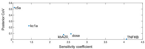
Figure 13: Sensitivity coefficients plotted against coefficient of variation in the NF-$\kappa$B system (left) and Drosophila clock $\Omega=300$ (right) (rows corresponding to standardisation by posterior mean and true value respectively).

The relation of parameter estimates to the sensitivity coefficients

We next wish to establish whether the sensitivity analysis could and/or should be used to guide parameter estimation. More specifically, we consider the relation between the sensitivity coefficients derived using the method described in section 4.1 and the posterior Coefficient of Variation (CoV, standard deviation/mean) of each parameter. Note that the prior CoV is $1$ for the priors used here.

Figure 13 shows the log10 overall sensitivity coefficients $\|{\bm{s}}_{j}\|$ plotted against posterior coefficients of variation for the two systems. The NF-$\kappa$B systems clearly shows a distinction between the three most sensitive parameters, having low CoV and those with low sensitivity. The Drosophila system shows less clear distinction across parameters, as all parameters estimated have comparatively high sensitivities. To investigate this further, we run the PT MCMC with $\beta_{k}\in\{1,0.5,0.3,0.1\}$ considering various parameters for estimation, leaving the rest fixed. We see a clear distinction between the case where the 5 parameters with the highest overall sensitivity coefficients $\|{\bm{s}}_{j}\|$ are estimated compared to estimating the 5 parameters with the lowest $\|{\bm{s}}_{j}\|$ (see Figure 14a). The parameters with low sensitivity have much larger posterior CoV compared to those with high sensitivity. Figure 15 shows that parameter chains wonder around the parameter space, accepting various parameter combinations that form low modes in the posterior distribution. That comes in stark contrast to the unimodal posteriors that arise for the parameters with high $\|{\bm{s}}_{j}\|$ (see Figure 16). A difference between posterior CoV for parameters with low $\|{\bm{s}}_{j}\|$ and high $\|{\bm{s}}_{j}\|$ is also seen when ten parameters are estimated, albeit here is smaller. A general tendency for higher posterior CoV as the sensitivity coefficient $\|{\bm{s}}_{j}\|$ becomes smaller is observed in Figure 14c where more parameters are estimated.

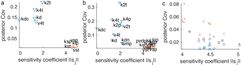
Figure 14: Posterior Coefficients of Variation against the overall sensitivity coefficients $\|{\bm{s}}_{j}\|$ for different runs of PT MCMC. The results in (a) are for a run with the 5 parameters of highest (red crosses) and lowest (blue triangles) $\|{\bm{s}}_{j}\|$ are estimated, in (b) 10 parameters of highest (red triangles) and lowest (blue triangles) $\|{\bm{s}}_{j}\|$ are estimated, and (c) 15 (blue circles) and 20 (red crosses) parameters of highest $\|{\bm{s}}_{j}\|$.

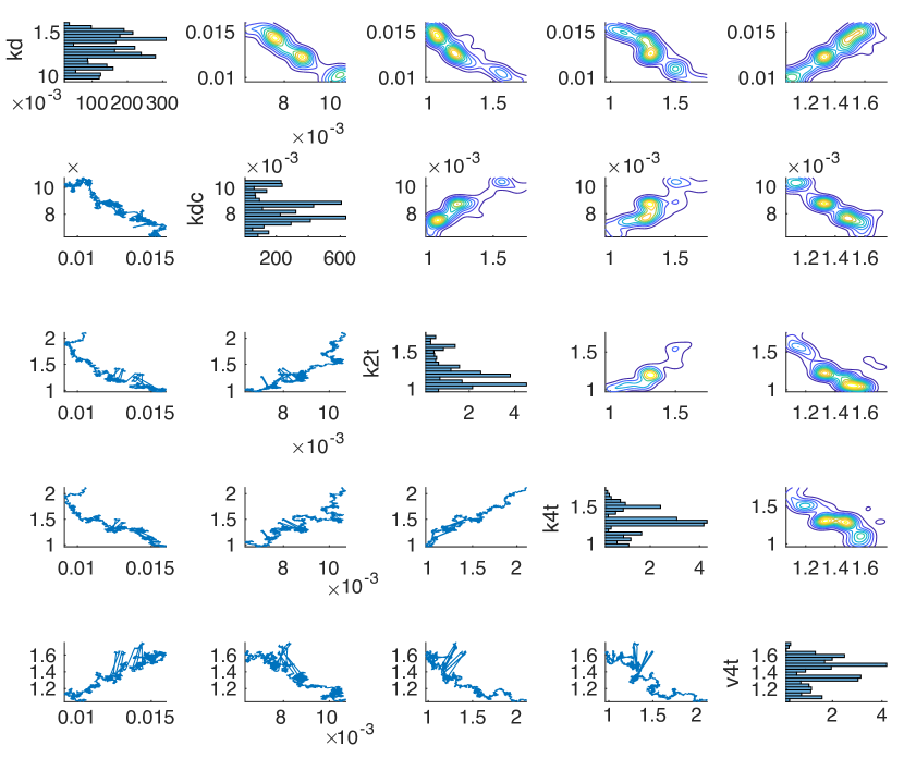
Figure 15: Posterior inference for the Drosophila circadian clock system ($\Omega=300$ estimating 5 parameters. The histograms (main diagonal) of each parameter, and the MCMC chains (lower diagonal) and contour plots of posterior distribution (upper diagonal) of pairs of parameters are presented. For this parameters with low sensitivity, the posteriors present multimodality with the chains exploring various parameter combinations.

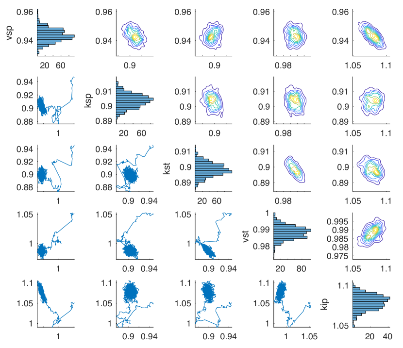
Figure 16: Posterior inference for the Drosophila circadian clock system ($\Omega=300$ estimating 5 parameters. The histograms (main diagonal) of each parameter, and the MCMC chains (lower diagonal) and contour plots of posterior distribution (upper diagonal) of pairs of parameters are presented. For this parameters with high sensitivity, the posteriors quickly converge to their unimodal posteriors.

6.3 Comparison to restarting LNA of Fearnhead et al. (2014)

We compare our approach to that of Fearnhead et al. (2014), which also uses the LNA as the underlying model. The difference is that the restarting LNA Kalman Filter replaces the phase correction implemented in our method with a resetting of the initial condition of the ODE in (2.2) that sets the stochastic component $\bm{\xi}_{t_{i}}$ to zero before transition from time $t_{i}$ to $t_{i+1}$. The restarting LNA makes no assumptions on the dynamics of the LNA, and therefore could potentially be applied to systems of any dynamics. The rough idea is to make LNA steps short transitions by frequently resetting of initial conditions; since LNA is accurate in short transitions this should improve its accuracy. The resetting of initial conditions of the ODE implies that the solutions of all the ODEs involved in the LNA are solved between each resetting times. The trajectory of the restarting LNA follows (in some sense) the (dynamic) posterior mean, even when this is rapidly changing, and it’s therefore smooth only between transitions. This is unlike the pcLNA that, which as we described in section 2, for a given parameter vector, solves the system once for all the observed time interval, and adjusts only the time-phase of the ODE solutions.

We implemented the same PT MCMC used above with the likelihood now computed under the restarting LNA described in Fearnhead et al. (2014), but all the remaining steps unchanged. We saw that the posterior distributions are similar to the pcLNA, with main difference the speed of implementation, which is about 2 times slower. The main factor for this slow down is the extra calls of the ODE solvers.

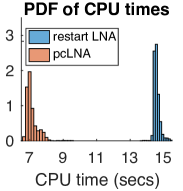
Figure 17: Histograms of the CPU times of one iteration in seconds for pcLNA and restarting LNA (see legend). The increase in CPU time with restarting LNA is roughly 2 fold.

7 Discussion

The proposed approach was highly successful in retrieving accurate estimates of simulated parameters from data in large stochastic non-linear dynamical systems with oscillations, conditional on the level of sensitivity of the model output to those parameters being sufficiently high. The sensitivity analysis was able to predict which parameters were estimable from observed data, across the tested simulation settings (different variables, varying Omega and Gillespe and pcLNA simulated data). These highly-parameterised systems have not previously been estimable due to the computational demand of calculating the conditional distributions of the state process at the desired timepoints. Our simulations have highlighted a variety of challenges of the systems, including (non-)identifiability, data resolution and multimodal distributions common to these types of systems.

We emphasise the importance of conducting sensitivity analysis on non-linear dynamical systems prior to conducting inference. Attempting to conduct inference in partially- or non-identifiable systems risks erroneous results, even for parameters that should be identifiable. In the case of the parallel tempering algorithm, posteriors marginals were similar to the priors specified on them but with too many non-identifiable parameters this may not remain the case. Our results also show the importance of considering the discrete time points that are used to conduct inference. In some instances these may be determined by the experimental set-up, but as modern sequencing technologies continue to advance, the choice of resolution and interrogation of the underlying continuous process will be increasingly important. Sensitivity analyses or inference should also allow for varying temporal resolutions in the data (Baggenstoss, 2018, e.g.), particularly in the presence of observation errors.

We compared several MCMC algorithms for conducting inference and found that despite improvements in sample sizes, the random walk Metropolis and geometric algorithms struggled to bypass bifurcations in parameter space and hence underestimate posterior uncertainty in marginal distributions. Our approach using the tempered algorithm was able to account for bifurcations in parameter space and also highlight alternative parameter combinations consistent with the data that warranted further study. Girolami and Calderhead (2011) highlight that extending the manifold MALA algorithm to a manifold Hamiltonian Monte Carlo (HMC) algorithm facilitates implementation within a parallel tempered algorithm and this may further improve the results found here. In particular, the improved convergence rate of parallel tempering combined with the improved local mixing of the geometric algorithms. It should be noted, however, that this does require significant increased computational power in the calculation of the derivatives of the metric tensor (i.e. FIM) and improvements in efficiency could be hindered by this.

We have shown that the ability to estimate parameters accurately and precisely varies along a variety of axes within these stochastic models. Increasing number of large eigenvalues of the mechanistic model is shown empirically to be proportional to the number of estimable parameters in the model and the loadings of the principal eigenvalues are highly indicative of which parameters are estimable. Similarly, increasing stochasticity unsurprisingly hindered the ability to obtain more precise parameter estimates via uncertainty in the corresponding posterior marginals. In many experimental designs, it may not be feasible to measure all of the biological species and our results show this can hinder the estimation of some parameters, but others are still estimable if the sensitive outputs are still measured.

Our approach has made significant advances in the ability to conduct exact and fast Bayesian inference in high-dimensional stochastic systems of reaction networks, whilst being similarly applicable to other stochastic models based on stochastic differential equations, such as those found in epidemiology and population dynamics. Remaining challenges exist in improving optimal experimental design, as well as developing optimum block updating strategies for the parameters when single parameters may dominate.

Appendix

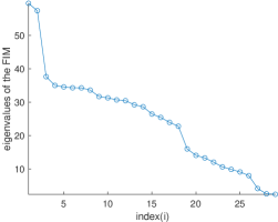
Figure 18: Eigenvalues (in log2 scale) of the FIM for the pcLNA model of the NF-$\kappa$B system with parameters in raw scale. The log2 of the eigenvalues is presented here. This is the same setting with Figure 4 but here all eigenvalues are reported.

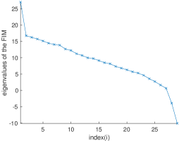
Figure 19: Eigenvalues (in log2 scale) of the FIM for the pcLNA model of the NF-$\kappa$B system with parameters in log-scale. This is the same setting with Figure 4 but here all eigenvalues are reported.

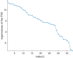
Figure 20: Eigenvalues (in log2 scale) of the FIM for the pcLNA model of the circadian clock system with parameters in log-scale. This is the same setting with Figure 4 but here all eigenvalues are reported.

References

-
Allen (2017)
Allen, L. J. S. (2017).
“A primer on stochastic epidemic models: Formulation,
numerical simulation, and analysis.”
Infectious Disease Modelling, 2: 128–142.
URL http://www.ncbi.nlm.nih.gov/pubmed/29928733http://www.pubmedcentral.nih.gov/articlerender.fcgi?artid=PMC6002090 - Ashall et al. (2009) Ashall, L., Horton, C. A., Nelson, D. E., Paszek, P., Harper, C. V., Sillitoe, K., Ryan, S., Spiller, D. G., Unitt, J. F., Broomhead, D. S., Kell, D. B., Rand, D. A., Sée, V., and White, M. R. H. (2009). “Pulsatile Stimulation Determines Timing and Specificity of NF-B-Dependent Transcription.” Science, 324(5924): 242–246.
- Baggenstoss (2018) Baggenstoss, P. M. (2018). “Acoustic Event Classification Using Multi-Resolution HMM.” In 2018 26th European Signal Processing Conference (EUSIPCO), 972–976.
- Beaumont (2003) Beaumont, M. A. (2003). “Estimation of Population Growth or Decline in Genetically Monitored Populations.” Genetics, 164(3): 1139–1160.
-
Boettiger (2018)
Boettiger, C. (2018).
“From noise to knowledge: how randomness generates novel
phenomena and reveals information.”
Ecology Letters, 21: 1255–1267.
URL http://doi.wiley.com/10.1111/ele.13085 -
Browning et al. (2020)
Browning, A. P., Warne, D. J., Burrage, K., Baker, R. E., and Simpson, M. J.
(2020).
“Identifiability analysis for stochastic differential
equation models in systems biology.”
Journal of The Royal Society Interface, 17(173): 20200652.
URL https://royalsocietypublishing.org/doi/abs/10.1098/rsif.2020.0652 - Burton et al. (2021) Burton, J., Manning, C. S., Rattray, M., Papalopulu, N., and Kursawe, J. (2021). “Inferring kinetic parameters of oscillatory gene regulation from single cell time-series data.” Journal of The Royal Society Interface, 18(182): 20210393.
- Chib and Greenberg (1995) Chib, S. and Greenberg, E. (1995). “Understanding the Metropolis-Hastings Algorithm.” American Statistician, 49: 327–335.
- Cover and Thomas (2006) Cover, T. M. and Thomas, J. A. (2006). Elements of Information Theory (Wiley Series in Telecommunications and Signal Processing). USA: Wiley-Interscience.
- DeFelice et al. (2019) DeFelice, M. M., Clark, H. R., Hughey, J. J., Maayan, I., Kudo, T., Gutschow, M. V., Covert, M. W., and Regot, S. (2019). “NF-B signaling dynamics is controlled by a dose-sensing autoregulatory loop.” Science Signaling, 12.
- Fearnhead et al. (2014) Fearnhead, P., Giagos, V., and Sherlock, C. (2014). “Inference for reaction networks using the linear noise approximation.” Biometrics, 70(2): 457–466.
- Finkenstädt et al. (2013) Finkenstädt, B., Woodcock, D. J., Komorowski, M., Harper, C. V., Davis, J. R. E., White, M. R. H., and Rand, D. A. (2013). “Quantifying intrinsic and extrinsic noise in gene transcription using the linear noise approximation: an application to single cell data.” The Annals of Applied Statistics, 7(4): 1960–1982.
- Forger (2017) Forger, D. B. (2017). Biological clocks, rhythms, and oscillations: The theory of biological timekeeping. Cambridge (MA): MIT Press. MIT Press, Cambridge (MA).
-
Froda and Nkurunziza (2007)
Froda, S. and Nkurunziza, S. (2007).
“Prediction of predator–prey populations modelled by
perturbed ODEs.”
Journal of Mathematical Biology, 54(3): 407–451.
URL https://doi.org/10.1007/s00285-006-0051-9 - Gabriel et al. (2021) Gabriel, C. H., del Olmo, M., Zehtabian, A., Jäger, M., Reischl, S., van Dijk, H., Ulbricht, C., Rakhymzhan, A., Korte, T., Koller, B., Grudziecki, A., Maier, B., Herrmann, A., Niesner, R., Zemojtel, T., Ewers, H., Granada, A. E., Herzel, H., and Kramer, A. (2021). “Live-cell imaging of circadian clock protein dynamics in CRISPR-generated knock-in cells.” Nature Communications, 12: 3796.
- Gard and Kannan (1976) Gard, T. C. and Kannan, D. (1976). “On a stochastic differential equation modeling of prey-predator evolution.” Journal of Applied Probability, 13(3): 429–443.
- Gillespie (1977) Gillespie, D. T. (1977). “Exact stochastic simulation of coupled chemical reactions.” The Journal of Physical Chemistry, 81(25): 2340–2361.
-
Gillespie (1992)
— (1992).
“A rigorous derivation of the chemical master equation.”
Physica A: Statistical Mechanics and its Applications, 188:
404–425.
URL http://www.sciencedirect.com/science/article/pii/037843719290283Vhttps://www.sciencedirect.com/science/article/pii/037843719290283V -
Gillespie (2000)
— (2000).
“The chemical Langevin equation.”
The Journal of Chemical Physics, 113: 297–306.
URL http://scitation.aip.org/content/aip/journal/jcp/113/1/10.1063/1.481811 - Gillespie and Petzold (2003) Gillespie, D. T. and Petzold, L. R. (2003). “Improved leap-size selection for accelerated stochastic simulation.” The Journal of Chemical Physics, 119.