Singularities of regular black holes and the monodromy method for asymptotic quasinormal modes

Abstract

We use the monodromy method to investigate the asymptotic quasinormal modes of regular black holes based on the explicit Stokes portraits. We find that, for regular black holes with spherical symmetry and a single shape function, the analytical forms of the asymptotic frequency spectrum are not universal and do not depend on the multipole number but on the presence of complex singularities and the trajectory of asymptotic solutions along the Stokes lines.

1 Introduction

Regular black holes (RBHs) are a collection of black holes (BHs) that do not have singularities in spacetime, especially at their centers [1, 2, 3], i.e., all the curvature invariants of BHs, such as the Kretschmann scalar, are finite everywhere. This definition is related to Markov’s limiting curvature conjecture [4, 5], which states that the curvature invariants should be restricted by a universal value. There is also a well-known definition of the regularity of spacetime through the completeness of null and timelike geodesics [6, 7]. Unfortunately, these two definitions are not equivalent. Some BHs have finite curvature everywhere, but the spacetime contain incomplete geodesics, e.g., the Taub–NUT BH [8, 9]. Others are the opposite, namely, the geodesics in spacetime are complete everywhere, but the curvatures can be divergent in a certain area, e.g., a wormhole model in Ref. [10].

The study of RBHs dates back to Sakharov and Gliner [11, 12] and is interesting because RBHs are not restricted by the Penrose singularity theorem [13]. The spacetime singularity can be avoided by replacing the center with a de Sitter core[14]. The first RBH model was implemented by Bardeen [15], in which a RBH was obtained by a formal modification of the Schwarzschild BH. A significant breakthrough came in 1998, when Ayon-Beato and Garcia offered the first interpretation of matter, in terms of classical fields, that generates RBHs [1]. In their follow-up research [16], Ayon-Beato and Garcia also showed that the Bardeen BH can be interpreted by the nonlinear magnetic monopole. This idea was generalized further by Fan and Wang [17]. Now, all spherically symmetric RBHs with singular shape functions can be interpreted in the context of nonlinear electrodynamics, i.e., given the metric of a RBH, the Lagrangian of matter generation can be derived in terms of electrodynamic field strength. These results stimulated further research on RBHs, including not only their construction [18, 2, 19, 20, 21, 22, 23], but also the interpretation of RBH models [24, 25, 26, 27] and various physical phenomena in RBHs spacetime, such as BH thermodynamics [28, 29], BH shadows [30, 31], and quasinormal modes (QNMs)[32, 33, 34].

The research program for RBHs may differ from that of traditional BHs with singularities. In the latter, the full action of the system is first given, and the BH solution can then be solved using the Euler–Lagrange equation obtained from the variational principle. In the former, the metric of a RBH can be constructed from the aspect of finite curvature invariants. Subsequently, information on the matter source can be deduced within a specific context that facilitates the solution, such as nonlinear electrodynamics [35, 36, 37, 38], in the presence of a phantom scalar field [25, 39] or modified gravity[40, 41].

The area/entropy spectrum of BHs is known to be related to their QNMs [42, 39] and, specifically, to the imaginary component of QNMs in the large damping limit, i.e. asymptotic QNMs (AQNMs) [43]. In other words, the area/entropy spectrum is obtained via the Bohr–Sommerfeld quantization of an adiabatic invariant [44] constructed using the AQNMs, whereas the AQNMs of BHs can be determined by the so-called monodromy approach [45], in which singularities and Stokes lines play crucial roles [46]. As a result, studying the quantum entropy spectrum of RBHs requires a thorough understanding of AQNMs. The goal of this study is to investigate the AQNMs of RBHs in greater detail using a clear Stokes diagram.

For a traditional BH with a singularity at the center, such as the Schwarzschild BH, the Stokes lines emit from the central singularity. Thus, when the asymptotic solutions of the Regge–Wheeler master equation rotate from one Stokes line to another around the zero point of the radial coordinate (i.e., the center of the BH), the change is not trivial, and the monodromy along a closed Stokes line will give an analytical expression for AQNMs, see e.g. [47, 48].

For a RBH [3], the zero point of the metric is no longer singular in most cases, and the corresponding Stokes lines do not converge to that point, which implies that the rotation of the asymptotic solution around the zero point is trivial. Several attempts have been made by ignoring this problem [32, 49], where the Stokes lines of RBHs are borrowed from Reissner–Nordström (RN) or RN-like BHs based on the similarity of the metrics at infinity, and the asymptotic frequencies of these models have a universal form, see Eq.(12) in [32]. In other words, to obtain the monodromy, the RBH is regarded as a singular BH. Therefore, one may ask what the true Stokes lines of RBHs are and what the monodromy based on these is. In the current study, we give a detailed discussion.

This paper is organized as follows: In Sec. 2, we illustrate and classify the singularities of RBHs from the perspective of complex analysis, which can be regarded as a prelude for the calculation of AQNMs in the subsequent sections.

After introducing an alternative approach to displaying the Stokes diagram in Sec. 3, we calculate the AQNMs of RBHs that still have complex singularities as the poles of the shape functions based on the explicit Stokes portrait in Sec. 4. Sec. 5 contains other examples in which the RBHs have essential singularities or no singularities at all.

We also provide a brief comparison of the monodromy method and complex WKB method from the perspective of the Stokes portrait in Sec. 6, and a conclusion is given in Sec. 7.

2 Singularities of regular black holes

Let us start with spherically symmetric BHs with a single shape function $f(r)$ in the metric

$$g_{\mu\nu}=\operatorname{diag}\{-f(r),f^{-1}(r),r^{2},r^{2}\sin^{2}(\theta)\},$$ (1)

where we suppose that $f(r)$ is of the following form:

$$f(r)=1-\frac{2M}{r}\sigma\left(r\right).$$ (2)

Here, $M$ is the BH mass, and $\sigma(r)$ is a dimensionless function of the radial coordinate. A BH with the metric in Eq. (1) is regular if all its curvature invariants referring to the Riemann tensor are finite for $r\in[0,\infty)$, e.g. the Ricci curvature $R\coloneqq g^{\mu\nu}R_{\mu\nu}$ and Weyl curvature $W\coloneqq W_{\mu\nu\alpha\beta}W^{\mu\nu\alpha\beta}$, where $R_{\mu\nu}$ and $W_{\mu\nu\alpha\beta}$ are the Ricci and Weyl tensors respectively. From a physical perspective, “regularity” implies that there are no gravitational singularities within the BH horizons. Furthermore, all RBHs with the Eq. (1) metric can be interpreted as magnetic monopoles [17].

For the Eq. (1) metric, we can compute the Ricci and Weyl curvatures

$$R=\frac{2M}{r^{2}}\left(2\sigma^{\prime}+r\sigma^{\prime\prime}\right),\quad W=\frac{4M^{2}}{3r^{6}}\left[r\left(r\sigma^{\prime\prime}-4\sigma^{\prime}\right)+6\sigma\right]^{2},$$ (3)

from which we note that the singularities of the curvature invariants are unavoidable if the function $f(r)$ has singularities in $r\in[0,\infty)$. Additional restricted conditions for $f(r)$ that guarantee the finiteness of the curvature invariants at $r=0$ have been discussed, for example, in Ref. [21, 5, 17, 29].

Furthermore, the Ricci and Weyl curvatures can be simplified if we replace $\sigma\to s_{1}(r)/(2Mr)$ for $R$ and $\sigma\to\sqrt{3}r^{2}s_{2}(r)/(2M)$ for $W$, yielding

$$R=\frac{s_{1}^{\prime\prime}(r)}{r^{2}},\qquad W=r^{2}s_{2}^{\prime\prime}(r)^{2},$$ (4)

which provides convenience when constructing RBHs with various types of mathematical singularities.

In contrast, according to the monodromy method, as we compute the AQNMs for BHs with gravitational singularities at $r=0$, such as Schwarzschild and RN BHs, the radial coordinate $r$ in the Regge–Wheeler master equation is analytically continued into the complex plane, and the physical singularities (gravitational singularities and BH horizons) play a key role [45]. Therefore, it is natural to wonder what to do when dealing with the AQNMs of RBHs if there are no gravitational singularities.

In fact, the mechanisms for removing the singularities of BHs are considerbaly different from each other from the perspective of complex analysis, and these differences are reflected in the calculations of AQNMs. Therefore, we first divide the RBHs into three classes according to the types of singularities of the curvature invariants after analytically continuing the radial coordinate into the complex plane:

1. The curvature invariants are entire functions of $r$, i.e., they have either no singularities on the entire complex plane $\mathbb{C}$ or removable singularities at $r=0$.

2. The curvature invariants are meromorphic functions on $\mathbb{C}$. In other words, the point $r=0$ is a regular point; however, the singularities (as poles) still exist and are located in the ranges beyond the non-negative axis of $r$, i.e., the singularities of the curvature invariants are dragged into the non-physical domain.

3. $r=0$ is an essential singularity of the curvature invariants. Via Picard’s great theorem [51], RBHs with an essential singularity at $r=0$ must have infinitely many complex horizons on any punctured neighborhood of $r=0$.

Several BH examples can be used to help understand this classification. First, we propose a RBH model with

$$\sigma=\frac{Mr}{Q^{2}}-\frac{Q^{2}}{16Mr}\sin^{2}\left(\frac{4Mr}{Q^{2}}\right),$$ (5)

where $Q$ is a parameter introduced to balance the dimensions.

To reduce the parameters, we rescale $r\to l^{2/3}(2M)^{1/3}z$ and $Q\to 2^{7/6}l^{1/3}M^{2/3}$, where $z$ is a dimensionless radial coordinate, and $l$ is a parameter of length dimension and is expected to be the Planck length or of the same order. Then, the horizons $z_{\rm H}$ can be determined using the equation

$$\lambda\coloneqq\left(\frac{l}{2M}\right)^{2/3}=\frac{1}{4}-\frac{\sin^{2}(z_{\rm H})}{4z_{\rm H}^{2}}.$$ (6)

Because sine is a transcendental function, there must be infinitely many complex horizons for any $\lambda\in\mathbb{R}$ and no Picard exceptional values according to Picard’s little theorem [51, 52]; however, the number of complex horizons is finite in any circle around $z=0$.

We also note that the number of physical horizons increases discretely with increasing $\lambda$ in the interval $(0.238,1/4]$. The model has only one horizon when $\lambda\lesssim 0.238$, two horizons when $\lambda\approx 0.238$, and an infinite number of horizons when $\lambda=1/4$. The Ricci and Weyl curvatures can be computed as

$$R=\frac{\sin^{2}(z)}{l^{2}z^{2}},\qquad W=\frac{\sin^{2}(z)}{3l^{4}z^{8}}\left[\left(z^{2}-3\right)\sin(z)+3z\cos(z)\right]^{2},$$ (7)

where $z=0$ is a removable singularity belonging to the first type above. Moreover, it is easy to verify that this model meets the dominant energy condition (DEC) [53].

To understand another case in the first type, we propose a model of a RBH with

$$\sigma=\mathrm{e}^{-\frac{r}{l}}\left(\frac{6l}{r}+\frac{r}{l}+4\right)-\frac{6l}{r}+2.$$ (8)

Under the rescalings $r\to l^{2/3}(2M)^{1/3}z,l\to l^{2/3}(2M)^{1/3}$, we can fix the horizons via

$$\lambda=\mathrm{e}^{-z_{\rm H}}\left(\frac{6}{z_{\rm H}^{2}}+\frac{4}{z_{\rm H}}+1\right)-\frac{6}{z_{\rm H}^{2}}+\frac{2}{z_{\rm H}},$$ (9)

where $\lambda$ is formally the same as defined in Eq. (6). When $\lambda\lesssim 0.173$, there are two physical horizons, whereas there are infinitely many complex horizons. In addition, the DEC of this model also holds. The typical curvature invariants are then

$$R=\frac{\mathrm{e}^{-z}}{l^{2}},\qquad W=\frac{\mathrm{e}^{-2z}}{3l^{4}z^{8}}\left[12\mathrm{e}^{z}(z-6)+z^{4}+6z^{3}+24z^{2}+60z+72\right]^{2},$$ (10)

which are surely finite in the physical domain. In contrast, as we analytically continue $z$ into the entire complex plane, although there are no singularities in the finite range divergence occures at complex infinity owing to the Stokes phenomenon of the function $\mathrm{e}^{-z}$. In other words, as $z$ approaches infinity along a path restricted in the sector

$$\frac{\uppi}{2}<\arg(z)<\frac{3\uppi}{2},$$ (11)

the curvature invariants become divergent, namely complex infinity is an essential singularity of the model.

Now, we turn to the Hayward BH [2] with $\sigma=r^{3}/\left(r^{3}+2Ml^{2}\right)$, where $l/(2M)\ll 1$. The curvature invariants of this model are finite in the domain $r\in[0,\infty)$. However, after analytically continuing $r$ into the complex plane, the Weyl curvature

$$W=\frac{48M^{2}r^{6}\left(r^{3}-4l^{2}M\right)^{2}}{\left(2l^{2}M+r^{3}\right)^{6}}$$ (12)

starts having three singularities in the non-physical domain, which are determined using the algebraic equation $2l^{2}M+r^{3}=0$. More precisely, the Hayward BH has three poles after the analytical continuation. This is what we have in the second type, i.e., the singularities are hidden in the non-physical domain.

Furthermore, we can determine that all three singularities are located in the outermost horizons. The proof is a typical application of Rouché’s theorem [51]. First, we note from $2l^{2}M+r^{3}=0$ that all the singularities are located on a circle with the radius $\absolutevalue{r}=(2Ml^{2})^{1/3}$. Second, we can rewrite $f(r)=0$ as $r^{3}-2Mr^{2}+2Ml^{2}=0$, i.e., we obtain three complex horizons using the fundamental theorem of algebra. Third, on the circle $\absolutevalue{r}=(2Ml^{2})^{1/3}+\epsilon$, where $\epsilon\ll(2Ml^{2})^{1/3}$, we have $\absolutevalue{2Mr^{2}}>\absolutevalue{r^{3}}+\absolutevalue{2Ml^{2}}$ if $l/2M<1/(2\sqrt{2})\approx 0.35$ and $\epsilon/(2M)<\left(\sqrt{5}-1\right)/4\approx 0.31$. Finally, because $l/(2M)\ll 1$, we can conclude that there are two horizons in the circle $\absolutevalue{r}=(2Ml^{2})^{1/3}+\epsilon$ by applying Rouché’s theorem. In other words, the three complex horizons are sandwiched between the outermost and next to outermost horizons.

At last, the widely discussed model [21] with $\sigma(r)=\exp[-P^{2}/(2Mr)]$ belongs to the third type. After rescalings $r\to l^{2/3}\sqrt[3]{2M}z,P\to\sqrt[3]{l}(2M)^{2/3}$, its curvature invariants can be represented by

$$R=\frac{\mathrm{e}^{-1/z}}{l^{2}z^{5}},\qquad W=\frac{\mathrm{e}^{-2/z}}{3l^{4}z^{10}}[6(z-1)z+1]^{2}$$ (13)

where $z=0$ becomes an essential singularity after analytical continuation into the complex plane. A detailed discussion on this model is given in Sec. 5.1.

We end this section with a comment on constructing physical RBHs, Eqs. (5) and (8). Here, “physical” implies that the RBHs must obey the DEC [53]. Instead of the traditional method of selecting the well-behaved $\sigma$ [37, 5], we start with the curvature invariants Eqs. (3) and (4) directly, and choose strictly positive and finite functions as curvatures, solving $\sigma$-functions inversely from the differential equations. The “strict positivity” of Ricci curvature is a minimum requirement for satisfying the DEC, whereas the “finiteness” is the regularity in $r\in[0,\infty)$ and asymptotic flatness at infinity in their given sense. This process apparently provides an efficient approach to establishing physical RBHs, and it has indeed helped us create a series of models.

However, several problems in the process must to be treated carefully. For example, the existence of horizons and the integrality of $\sigma$. In other words, the $\sigma$-functions obtained from this method do not always provide horizons for the models. Because these problems go beyond the scope of the current study, we leave them for future research.

Furthermore, in this study, we concentrate on not only physical RBHs, but also non-physical models within the framework of Einstein’s gravity to focus on how the singularities of RBHs affect the spectrum of ANMQs.

3 Asymptotic quasinormal modes of regular black holes

3.1 Perturbation of a massless scalar field

The perturbation of a BH can be realized by laying a probing field onto the BH spacetime [48]. For a massless scalar field without backreaction, the perturbation reduces to the propagation equation of a scalar field,

$$\frac{1}{\sqrt{-g}}\partial_{\nu}\left(g^{\mu\nu}\sqrt{-g}\partial_{\mu}\Psi\right)=0.$$ (14)

In the spherically symmetric spacetime given by Eq. (1), we can substitute the ansatz $\Psi=\mathrm{e}^{-\mathrm{i}\omega t}Y_{l}(\theta,\phi)r^{-1}\psi(r)$ and then select the radial component

$$f\partial_{r}\left(f\partial_{r}\psi\right)+\left(\omega^{2}-V\right)\psi=0,\quad V=f\left[\frac{l(l+1)}{r^{2}}+\frac{f^{\prime}}{r}\right],$$ (15)

which is a second order differential equation. Or in the canonical form, we have

$$\psi^{\prime\prime}(r)+p\psi^{\prime}+q\psi=0,$$ (16)

where

$$p=\frac{f^{\prime}}{f},\qquad q=\frac{\omega^{2}-V}{f^{2}}.$$ (17)

Then, substituting the shape function, Eq. (2), the effective potential $V$ can be represented in terms of $\sigma$ and its derivatives

$$V=\frac{l(l+1)}{r^{2}}+V_{\rm reg},$$ (18)

where

$$V_{\rm reg}=-2l(l+1)M\frac{\sigma(r)}{r^{3}}+2M\frac{\sigma(r)}{r^{2}}-2M\frac{\sigma^{\prime}(r)}{r},$$ (19)

is a regular function at $r=0$ when $r\in[0,\infty)$, because for RBHs, $\sigma\sim O(r^{3})$ as $r\to 0$ [21, 5, 17, 29]. Thus, for any BHs without degenerate horizons (i.e., the horizons are the simple roots of the algebraic equation $f(r)=0$), one may find that $r=0$ and horizons are regular singular points of the master equation Eq. (16).

Furthermore, to diagonalize Eq. (16), we can define the tortoise coordinate by an indefinite integral,

$$z=\int\frac{\mathrm{d}r}{f(r)},$$ (20)

or the solution of the differential equation

$$\frac{\mathrm{d}z}{\mathrm{d}r}=\frac{1}{f(r)}.$$ (21)

The master equation, Eq. (16), then becomes

$$\left\{\frac{\mathrm{d}{}^{2}}{\mathrm{d}z^{2}}+\omega^{2}-V[r(z)]\right\}\psi(z)=0,$$ (22)

The QNMs are the solutions of Eq. (22) under the following boundary conditions:

$$\begin{split}\psi&\sim\mathrm{e}^{-\mathrm{i}\omega z},\quad z\to-\infty;\\ \psi&\sim\mathrm{e}^{\mathrm{i}\omega z},\quad z\to\infty.\end{split}$$ (23)

Thus, the high damping limit of QNMs will be defined as AQNMs, i.e., $\absolutevalue{\imaginary(\omega)}\gg\absolutevalue{\real(\omega)}$ as the overtone number approaches infinity for BHs with asymptotic flatness, see e.g., Refs. [47, 48].

Our goal in the current section is to find the AQNMs of Eq. (22) using an asymptotic analysis known as the monodromy method, in which the Stokes lines play a pivotal role. Therefore, before studying the AQNMs of specific models, let us take a close look at the geometry of Stokes lines. A detailed illustration of the monodromy method can be found in Refs. [45, 46, 54].

3.2 Stokes portraits for black holes

To understand the geometric aspects of Stokes lines, we first extend the radial coordinate $r$ into the complex plane and explicitly rewrite it with its real and imaginary components $x$ and $y$. We can then recast Eq. (20) as

$$z(x,y)\coloneqq\int^{x+\mathrm{i}y}\frac{\mathrm{d}r}{f(r)},$$ (24)

where the tortoise coordinate $z$ is also complex in general. Based on this representation, the real and imaginary parts of $z(x,y)$ can be regarded as two surfaces, and $z(x,y)=C$ are two groups of contours on each surfaces, i.e.

$$\real[z(x,y)]=c_{1},\qquad\imaginary[z(x,y)]=c_{2},\qquad C=c_{1}+\mathrm{i}c_{2}.$$ (25)

The Stokes lines are defined as the zero-contours, $\real[z(x,y)]=0$, on the first surface [45]. The Stokes lines must be symmetric with respect to the $y$-axis, i.e.

$$\real[z(x,y)]=\frac{1}{2}\left[z(x,y)+z(x,-y)\right]=\real[z(x,-y)].$$ (26)

The one-form $\mathrm{d}\real[z]$ corresponds to a vector field,

$$\mathrm{d}\real[z]=\real\left[1/f(x+\mathrm{i}y)\right]\mathrm{d}x-\imaginary\left[1/f(x+\mathrm{i}y)\right]\mathrm{d}y,$$ (27)

whereas its Hodge dual (with respect to the Euclidean metric) or the Stokes field [55]

$$\star\!\mathrm{d}\real[z]=\imaginary\left[1/f(x+\mathrm{i}y)\right]\mathrm{d}x+\real\left[1/f(x+\mathrm{i}y)\right]\mathrm{d}y$$ (28)

is tangent to the contours at each point. In the following, we also use the component notation to represent the Stokes field, i.e.

$${\bm{V}}_{\rm st}=\left\{\imaginary\left[1/f(x+\mathrm{i}y)\right],\;\real\left[1/f(x+\mathrm{i}y)\right]\right\}.$$ (29)

Moreover, it is easy to verify that both the divergence and curl of the Stokes fields are constantly zero, i.e. $\star\mathrm{d}\star(\star\mathrm{d}\real[z])=0=\star\mathrm{d}\,(\star\mathrm{d}\real[z])$. In other words, the Stokes field $\star\mathrm{d}\real[z]$ is a harmonic one-form [56] because $z(r)$ is a holomorphic function, and its real and imaginary parts satisfy the Cauchy–Riemann equations.

The critical points of the Stokes field are defined as a set of points $\{(x,y)|\star\mathrm{d}\real[z(x,y)]=0\}$, i.e., the zeros of $1/f(r)=0$ on the complex plane of $r\in\mathbb{C}$. Meanwhile, the critical points of the field are also the singular points [57] of the Stokes lines. Then, one can immediately deduce a fact about the point $r=0$: the origin $r=0$ is a critical point for singular BHs but not for RBHs, which implies that the Stokes lines of singular BHs converge to (or emit from) zero, whereas for RBHs, the convergence points may not include $r=0$.

Let us first review two integrable examples, Schwarzschild and RN BHs. The two plots in Fig. 1 show the Stokes surfaces $\real[z(x,y)]$, where the peaks on the surfaces correspond to the horizons.

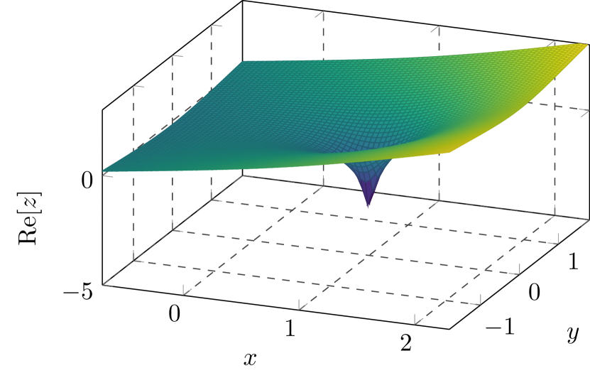
(a) Schwarzschild BH

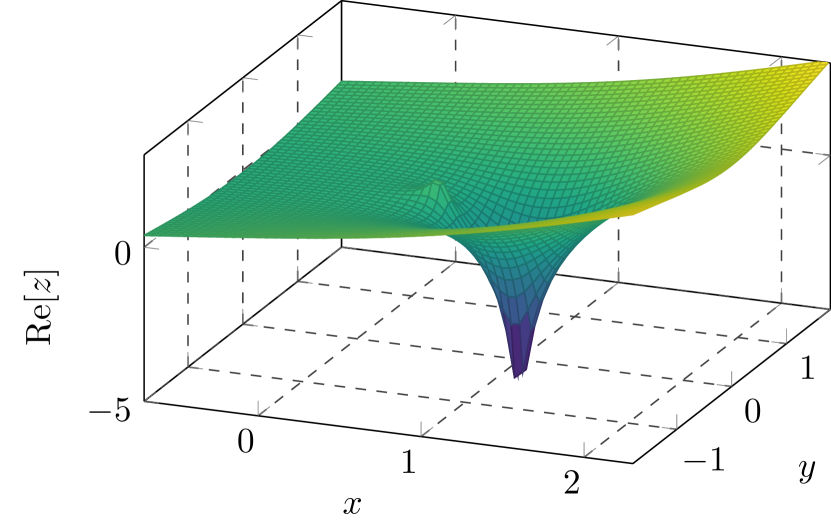
(b) Reissner–Nordström BH

Figure 1: Stokes surfaces $\real[z(x,y)]$.

Fig. 2 is a Stokes portrait/diagram, which consists of the vector field $\star\mathrm{d}\real[z]$ (blue), Stokes lines $\real[z]$=0 (yellow-brown) and complex horizons (purple). The Stokes lines can then be understood as the integral curves passing through the critical points in the Stokes portrait. Meanwhile, the complex horizons must be located inside the closed parts of the Stokes lines.

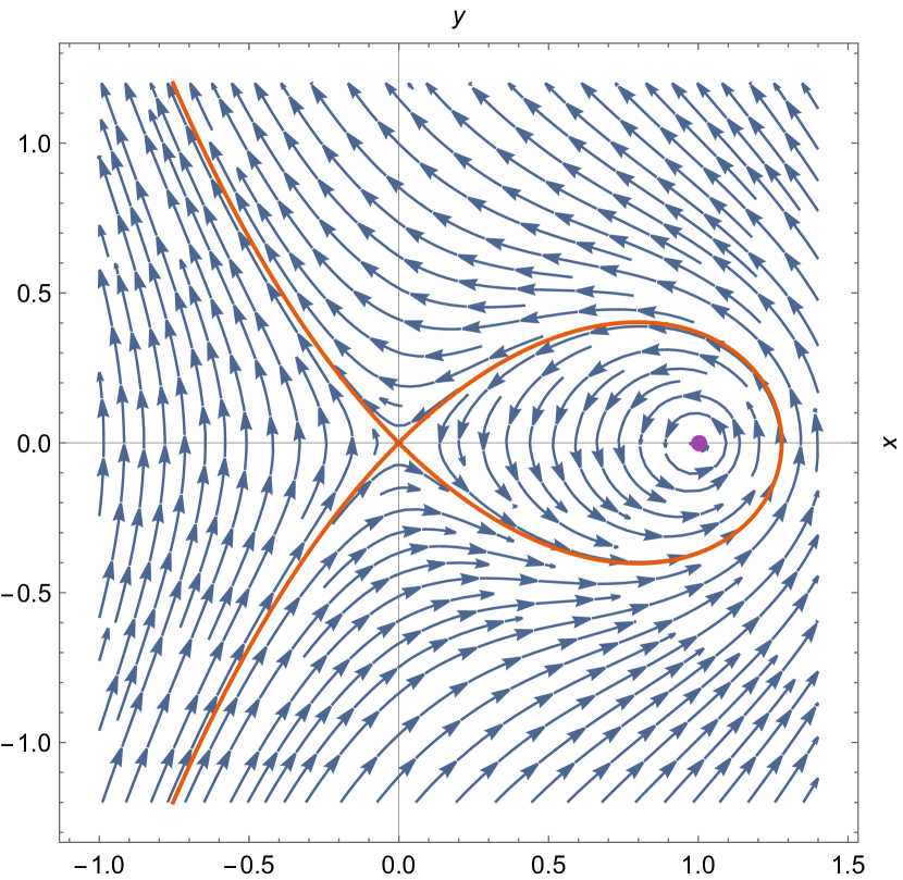
(a) Schwarzschild BH

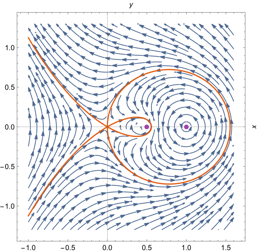
(b) Reissner–Nordström BH

Figure 2: Stokes diagrams in Cartesian coordinates; $\star\mathrm{d}\real[z(x,y)]$–blue vector fields, and the yellow-brown stream corresponds to the Stokes curves $\real[z(x,y)]=0$, where we set $k=1/2$ for RN BHs.

For the Schwarzschild BH with the shape function $f=1-1/r$, the Stokes vector field reads

$${\bm{V}}_{\rm st}=\left\{\frac{-y}{(x-1)^{2}+y^{2}},1+\frac{x-1}{(x-1)^{2}+y^{2}}\right\}.$$ (30)

The origin $r=(0,0)$ on the complex plane is a critical point, i.e., this Stokes line has a self-intersection at the origin. Near this point $(0,0)$, there is an approximation, ${\bm{V}}_{\rm st}\sim\left\{-y,-x\right\}$. The Stokes line of the Schwarzschild BH can be integrated out analytically,

$$(x-1)^{2}+y^{2}=\mathrm{e}^{-2x},$$ (31)

which is a transcendental curve. Moreover, around the origin $r=(0,0)$, Eq. (31) reduces to $y=\pm x$, i.e., there are $2\times 2=4$ lines emitting from the origin, and the angle between any two adjacent lines is $\uppi/2$.

For the RN BH with the shape function $f=(r-1)(r-k)/r^{2}$, where $1\geq k>0$, the Stokes field is

$$\begin{split}{\bm{V}}_{\rm st}=\Big{\{}&-\frac{xy[k(x-2)+x]+(k+1)y^{3}}{\left[(x-1)^{2}+y^{2}\right]\left[(x-k)^{2}+y^{2}\right]},\\ &\frac{-y^{2}\left(kx+k-2x^{2}+x\right)-(x-1)x^{2}(k-x)+y^{4}}{\left[(x-1)^{2}+y^{2}\right]\left[(x-k)^{2}+y^{2}\right]}\Big{\}}.\end{split}$$ (32)

The origin $r=(0,0)$ is also a self-intersecting point, near which there is an asymptotic behavior, ${\bm{V}}_{\rm st}\sim\left\{2xy/k,(x^{2}-y^{2})/k\right\}$. The Stokes line for this case is also a transcendental curve,

$$(x-1)^{2}+y^{2}=\mathrm{e}^{2(k-1)x}k^{-2k^{2}}\left[(k-x)^{2}+y^{2}\right]^{k^{2}}.$$ (33)

Around the origin $r=(0,0)$, $x=0$ and $x=\pm\sqrt{3}\,y$, i.e., there are $3\times 2=6$ lines emitting from the origin, and the angle between any two adjacent lines is $\uppi/3$.

Alternatively, to fix the angles between any two adjacent Stokes lines emitting from the critical point, we can also rewrite Eq. (28) in the polar coordinates $\{\rho,\phi\}$

$$\star\mathrm{d}\real[z]=\imaginary\left[\rho\mathrm{e}^{\mathrm{i}\phi}/f(\rho\mathrm{e}^{\mathrm{i}\phi})\right]\mathrm{d}\rho+\real\left[\mathrm{e}^{\mathrm{i}\phi}/f(\rho\mathrm{e}^{\mathrm{i}\phi})\right]\mathrm{d}\phi.$$ (34)

The angle relationship can then be directly visualized from the diagram in Fig. 3, i.e., the intersection of the Stokes lines with $\rho=0$ corresponds to the incident/exit angle of each line.

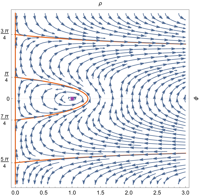
(a) Schwarzschild BH

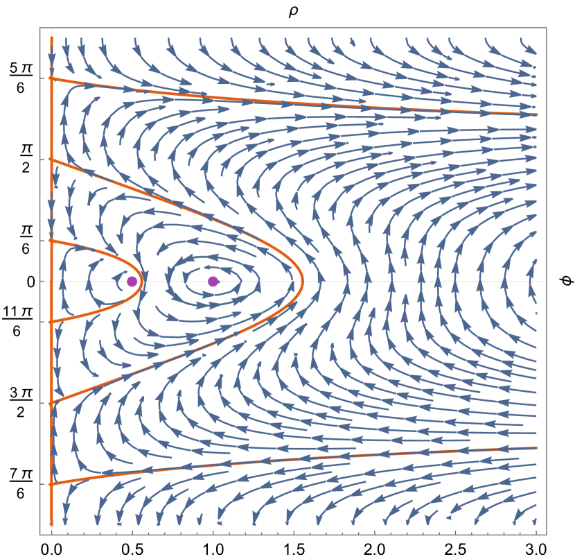
(b) Reissner–Nordström BH

Figure 3: Stokes diagrams in polar coordinates; $\star\mathrm{d}\real[z(\rho,\phi)]$–blue vector fields, and the yellow-brown stream corresponds to the exact Stokes lines. The parameter $k=1/2$ is adopted in the RN BH.

From an analytical point of view, the Stokes line of the Schwarzschild BH in polar coordinates becomes

$$1+\rho^{2}-2\rho\cos(\phi)=\exp\left[-2\rho\cos(\phi)\right]$$ (35)

where $\rho\geq 0$, and $2\uppi\geq\phi\geq 0$, see the plot in Fig. 3(a). To fix the angles of the emitting lines from origin, let us consider the corresponding vector field approaching $\rho\sim 0$, which gives

$$\frac{\mathrm{d}\rho}{\mathrm{d}\phi}\sim\rho\tan(2\phi)+O\left(\rho^{2}\right).$$ (36)

The stability condition $\mathrm{d}\rho/\mathrm{d}\phi\equiv 0$ implies that $\phi=\uppi n/2$ with $n\in\mathbb{Z}$. The angles of the emitting lines from origin can then be calculated as

$$\phi_{\rm st}=\frac{\uppi}{2}n+\frac{\uppi}{4},\qquad n\in\mathbb{Z}.$$ (37)

Similarly, we can compute the Stokes line and emitting angle for the RN BH arriving at

$$1+4\rho^{2}-4\rho\cos(\phi)=\left[\rho^{2}-2\rho\cos(\phi)+1\right]^{4}\exp\left[4\rho\cos(\phi)\right]$$ (38)

and $\phi_{\rm st}=\uppi n/3+\uppi/6$, $n\in\mathbb{Z}$, see the plot in Fig. 3(b).

4 Regular black holes with complex poles

4.1 Trajectory along the Stokes lines

Now, let us start with our first example of RBHs, the Bardeen BH [15], which can be generated by a nonlinear magnetic monopole. The Lagrangian of matter generation can be found in Ref. [35, 17],

$$\mathcal{L}=\frac{12}{\alpha}\frac{(\alpha\mathcal{F})^{5/4}}{(1+\sqrt{\alpha\mathcal{F}})^{5/2}},\quad\alpha=P^{3}/M,$$ (39)

where $\mathcal{F}=F_{\mu\nu}F^{\mu\nu}$ is the field strength, and $P$ and $M$ are the magnetic charge and mass parameters, respectively. We first rescale the shape function by

$$r\to Pr,\qquad M\to\frac{P}{2}M,$$ (40)

such that it becomes

$$f(r)=1-\frac{Mr^{2}}{\left(r^{2}+1\right)^{3/2}},$$ (41)

where all variables and parameters are dimensionless. The Stokes diagrams are displayed in Fig. 4.

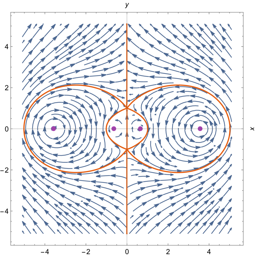
(a) Cartesian coordinates

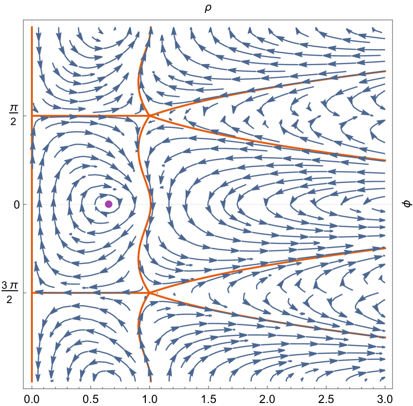
(b) Polar coordinates

Figure 4: Stokes diagrams for the Bardeen BH; $\star\mathrm{d}\real[z(x,y)]$–blue vector fields, and the yellow-brown curves correspond to the Stokes lines, where $M=4$.

Note that there are two critical points $\pm\mathrm{i}$, i.e., the singularities of the Bardeen BH are stretched from zero to the pure imaginary axis compared with the RN BH, see Fig. 2(b). This can also be understood from the Weyl curvature $W$, which is regular at zero but divergent at $\pm\mathrm{i}$, i.e., $\pm\mathrm{i}$ are the poles of the seventh-order,

$$W\sim\pm\frac{75\mathrm{i}M^{2}}{128P^{4}(r\mp\mathrm{i})^{7}}+O[(r\mp i)^{-6}].$$ (42)

Therefore, $\pm\mathrm{i}$ are the singular points of the master equation according to the effective potential, Eq. (18). Meanwhile, they are regular singular points because

$$(r\pm\mathrm{i})p=-\frac{3}{2}+O\left[(r\pm\mathrm{i})\right]\quad\text{and}\quad(r\pm\mathrm{i})^{2}q=\mp\frac{3}{2}\mathrm{i}(r\pm\mathrm{i})+O\left[(r\pm\mathrm{i})^{3/2}\right]$$ (43)

are regular at the corresponding points, where $p$ and $q$ are the coefficients in Eq. (17) of the master equation for the Bardeen BH. Furthermore, around these two critical points, there is an approximation of the tortoise coordinate

$$z\sim-\frac{4}{5M}\left(1\mp\mathrm{i}\right)(r\mp\mathrm{i})^{5/2},$$ (44)

and thus, there are five lines emitting from each critical point [58]. The polar diagram in Fig. 4(b) shows the angles of the Stokes lines passing through the zero point. Because $r=0$ is no longer a critical point, the angles at this point are trivial $\uppi$, the monodromy of the asymptotic solutions around $r=0$ is trivial.

To obtain information on the angles around the critical points $\pm\mathrm{i}$, we should apply the polar coordinates with the starting point at each critical point separately. Polar diagrams with starting points at $r=\mathrm{i}$ and $r=-\mathrm{i}$ are shown in Fig. 5. The angle between adjacent lines can be computed as $2\uppi/5$. Meanwhile, it must be emphasized that the line $\phi=\uppi/2$ emits from the lower point, whereas $\phi=3\uppi/2$ emits from the upper point. This information will help us determine a closed contour, which is applied to calculate the monodromy.

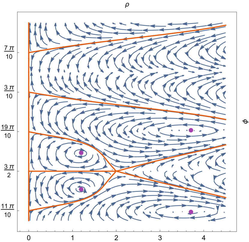
(a) Upper point

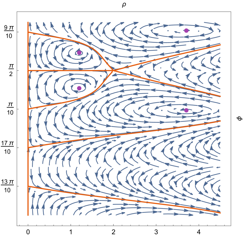
(b) Lower point

Figure 5: Stokes diagrams for the Bardeen BH in polar coordinates with starting points at each critical point.

For convenience of later discussions, let us denote the origin as $\mathcal{O}$, the upper and lower critical points as $\mathcal{A}$ and $\mathcal{B}$ respectively, and a point close to the right inner horizon as $\mathcal{C}$.

Now, let us start with the master equation at zero located on the Stokes line to calculate the AQNMs. Because the tortoise coordinate is approximately $z\sim r$ at $r=0$, we have

$$\psi^{\prime\prime}(z)+\left[\omega^{2}-\frac{l(l+1)}{z^{2}}\right]\psi(z)=0,$$ (45)

which gives the solution around $\mathcal{O}$

$$\psi_{\mathcal{O}}=Q_{+}\sqrt{2\uppi\omega z}J_{\frac{\nu}{2}}(\omega z)+Q_{-}\sqrt{2\uppi\omega z}J_{-\frac{\nu}{2}}(\omega z),$$ (46)

where $\nu=2l+1$, and $Q_{\pm}$ are two arbitrary constants. Then, considering the asymptotics of the Bessel functions

$$\sqrt{2\uppi\omega z}J_{\pm\frac{\nu}{2}}(\omega z)\sim 2\cos\left(\omega z-\alpha_{\pm}\right),\qquad\omega z>0$$ (47)

with $\alpha_{\pm}=\uppi\left(1\pm\nu\right)/4$, we find that at $-\mathrm{i}\infty$,

$$\psi_{-\mathrm{i}\infty}\sim\left(Q_{+}\mathrm{e}^{\mathrm{i}\alpha_{+}}+Q_{-}\mathrm{e}^{\mathrm{i}\alpha_{-}}\right)\mathrm{e}^{-\mathrm{i}\omega z}$$ (48)

and the condition

$$Q_{+}\mathrm{e}^{-\mathrm{i}\alpha_{+}}+Q_{-}\mathrm{e}^{-\mathrm{i}\alpha_{-}}=0,$$ (49)

where the boundary condition $\psi\to\mathrm{e}^{-\mathrm{i}z\omega}$ as $z\to\infty$ is used. To pass through $\mathcal{O}$, we must rotate $\uppi$ and hence obtain

$$\begin{split}\psi_{\mathcal{\hat{O}}}&=\mathrm{e}^{2\mathrm{i}\alpha_{+}}Q_{+}\sqrt{2\uppi\omega z}J_{\frac{\nu}{2}}(\omega z)+\mathrm{e}^{2\mathrm{i}\alpha_{-}}Q_{-}\sqrt{2\uppi\omega z}J_{-\frac{\nu}{2}}(\omega z)\\ &\sim\left(Q_{+}\mathrm{e}^{\mathrm{i}\alpha_{+}}+Q_{-}\mathrm{e}^{\mathrm{i}\alpha_{-}}\right)\mathrm{e}^{\mathrm{i}\omega z}+\left(Q_{+}\mathrm{e}^{3\mathrm{i}\alpha_{+}}+Q_{-}\mathrm{e}^{3\mathrm{i}\alpha_{-}}\right)\mathrm{e}^{-\mathrm{i}\omega z},\end{split}$$ (50)

which will be matched with the asymptotics at point $\mathcal{A}$

$$\begin{split}\psi_{\mathcal{A}}&\sim A_{+}\sqrt{2\uppi\omega(z-\mathrm{i})}J_{\frac{\nu}{2}}(\omega(z-\mathrm{i}))+A_{-}\sqrt{2\uppi\omega(z-\mathrm{i})}J_{-\frac{\nu}{2}}(\omega(z-\mathrm{i}))\\ &\sim\left(A_{+}\mathrm{e}^{\omega-\mathrm{i}\alpha_{+}}+A_{-}\mathrm{e}^{\omega-\mathrm{i}\alpha_{-}}\right)\mathrm{e}^{\mathrm{i}\omega z}+\left(A_{+}\mathrm{e}^{-\omega+\mathrm{i}\alpha_{+}}+A_{-}\mathrm{e}^{-\omega+\mathrm{i}\alpha_{-}}\right)\mathrm{e}^{-\mathrm{i}\omega z}.\end{split}$$ (51)

Here, we use $\hat{\mathcal{O}}$ to denote the position after rotation around $\mathcal{O}$. This notation also applies to the following discussion. The matching $\psi_{\mathcal{A}}\leftrightarrow\psi_{\mathcal{\hat{O}}}$ provides two more conditions:

$$\begin{split}Q_{+}\mathrm{e}^{\mathrm{i}\alpha_{+}}+Q_{-}\mathrm{e}^{\mathrm{i}\alpha_{-}}&=A_{+}\mathrm{e}^{\omega-\mathrm{i}\alpha_{+}}+A_{-}\mathrm{e}^{\omega-\mathrm{i}\alpha_{-}},\\ Q_{+}\mathrm{e}^{3\mathrm{i}\alpha_{+}}+Q_{-}\mathrm{e}^{3\mathrm{i}\alpha_{-}}&=A_{+}\mathrm{e}^{-\omega+\mathrm{i}\alpha_{+}}+A_{-}\mathrm{e}^{-\omega+\mathrm{i}\alpha_{-}}.\end{split}$$ (52)

To pass through $\mathcal{A}$, we also rotate $\uppi$ instead of $2\uppi$, which provides

$$\psi_{\mathcal{\hat{A}}}\sim\left(A_{+}\mathrm{e}^{\omega+\mathrm{i}\alpha_{+}}+A_{-}\mathrm{e}^{\omega+\mathrm{i}\alpha_{-}}\right)\mathrm{e}^{\mathrm{i}\omega z}+\left(A_{+}\mathrm{e}^{-\omega+3\mathrm{i}\alpha_{+}}+A_{-}\mathrm{e}^{-\omega+3\mathrm{i}\alpha_{-}}\right)\mathrm{e}^{-\mathrm{i}\omega z},$$ (53)

and the asymptotics as $z$ approaches the inner horizon are

$$\begin{split}\psi_{\mathcal{C}}&=C_{+}\sqrt{2\uppi\omega(z-\delta)}J_{\frac{\nu}{2}}(\omega(z-\delta))+C_{-}\sqrt{2\uppi\omega(z-\delta)}J_{-\frac{\nu}{2}}(\omega(z-\delta))\\ &\sim\left(C_{+}\mathrm{e}^{-\mathrm{i}\omega\delta+\mathrm{i}\alpha_{+}}+C_{-}\mathrm{e}^{-\mathrm{i}\omega\delta+\mathrm{i}\alpha_{-}}\right)\mathrm{e}^{\mathrm{i}\omega z}+\left(C_{+}\mathrm{e}^{\mathrm{i}\omega\delta-\mathrm{i}\alpha_{+}}+C_{-}\mathrm{e}^{\mathrm{i}\omega\delta-\mathrm{i}\alpha_{-}}\right)\mathrm{e}^{-\mathrm{i}\omega z},\end{split}$$ (54)

where $\delta=\mathrm{i}/(2T_{\rm H}^{-})$, and $T_{\rm H}^{-}$ is the “temperature” of the inner horizon. We use

$$\sqrt{2\uppi\omega(z-\delta)}J_{\pm\frac{\nu}{2}}(\omega(z-\delta))\sim 2\cos(\omega(z-\delta)+\alpha_{\pm}),\qquad(z-\delta)\omega\ll-1,$$ (55)

because $\omega(z-\delta)$ is negative on this branch. Then, the matching $\psi_{\mathcal{\hat{A}}}\leftrightarrow\psi_{\mathcal{C}}$ gives

$$\begin{split}C_{+}\mathrm{e}^{-\mathrm{i}\omega\delta+\mathrm{i}\alpha_{+}}+C_{-}\mathrm{e}^{-\mathrm{i}\omega\delta+\mathrm{i}\alpha_{-}}&=A_{+}\mathrm{e}^{\omega+\mathrm{i}\alpha_{+}}+A_{-}\mathrm{e}^{\omega+\mathrm{i}\alpha_{-}},\\ C_{+}\mathrm{e}^{\mathrm{i}\omega\delta-\mathrm{i}\alpha_{+}}+C_{-}\mathrm{e}^{\mathrm{i}\omega\delta-\mathrm{i}\alpha_{-}}&=A_{+}\mathrm{e}^{-\omega+3\mathrm{i}\alpha_{+}}+A_{-}\mathrm{e}^{-\omega+3\mathrm{i}\alpha_{-}}.\end{split}$$ (56)

Subsequently, we will rotate to the branch containing $\mathcal{B}$. We find

$$\psi_{\mathcal{\hat{C}}}\sim\left(C_{+}\mathrm{e}^{-\mathrm{i}\omega\delta+3\mathrm{i}\alpha_{+}}+C_{-}\mathrm{e}^{-\mathrm{i}\omega\delta+3\mathrm{i}\alpha_{-}}\right)\mathrm{e}^{\mathrm{i}\omega z}+\left(C_{+}\mathrm{e}^{\mathrm{i}\omega\delta+\mathrm{i}\alpha_{+}}+C_{-}\mathrm{e}^{\mathrm{i}\omega\delta+\mathrm{i}\alpha_{-}}\right)\mathrm{e}^{-\mathrm{i}\omega z},$$ (57)

which should be matched with the asymptotics at $\mathcal{B}$

$$\begin{split}\psi_{\mathcal{B}}&=B_{+}\sqrt{2\uppi\omega(z+\mathrm{i})}J_{\frac{\nu}{2}}(\omega(z+\mathrm{i}))+B_{-}\sqrt{2\uppi\omega(z+\mathrm{i})}J_{-\frac{\nu}{2}}(\omega(z+\mathrm{i}))\\ &\sim\left(B_{1}\mathrm{e}^{-\omega+\mathrm{i}\alpha_{+}}+B_{2}\mathrm{e}^{-\omega+\mathrm{i}\alpha_{-}}\right)\mathrm{e}^{\mathrm{i}\omega z}+\left(B_{1}\mathrm{e}^{\omega-\mathrm{i}\alpha_{+}}+B_{2}\mathrm{e}^{\omega-\mathrm{i}\alpha_{-}}\right)\mathrm{e}^{-\mathrm{i}\omega z}.\end{split}$$ (58)

The matching $\psi_{\mathcal{\hat{C}}}\leftrightarrow\psi_{\mathcal{B}}$ leads to another two conditions:

$$\begin{split}B_{1}\mathrm{e}^{-\omega+\mathrm{i}\alpha_{+}}+B_{2}\mathrm{e}^{-\omega+\mathrm{i}\alpha_{-}}&=C_{+}\mathrm{e}^{-\mathrm{i}\omega\delta+3\mathrm{i}\alpha_{+}}+C_{-}\mathrm{e}^{-\mathrm{i}\omega\delta+3\mathrm{i}\alpha_{-}},\\ B_{1}\mathrm{e}^{\omega-\mathrm{i}\alpha_{+}}+B_{2}\mathrm{e}^{\omega-\mathrm{i}\alpha_{-}}&=C_{+}\mathrm{e}^{\mathrm{i}\omega\delta+\mathrm{i}\alpha_{+}}+C_{-}\mathrm{e}^{\mathrm{i}\omega\delta+\mathrm{i}\alpha_{-}}.\end{split}$$ (59)

We then pass to the origin $\mathcal{O}$ again but in a different branch. To distinguish the solution of the master equation with the original one Eq. (46), let us denote it as $\widetilde{\psi}_{\mathcal{O}}$, i.e.

$$\begin{split}\widetilde{\psi}_{\mathcal{O}}&=\widetilde{Q}_{+}\sqrt{2\uppi\omega z}J_{\frac{\nu}{2}}(\omega z)+\widetilde{Q}_{-}\sqrt{2\uppi\omega z}J_{-\frac{\nu}{2}}(\omega z)\\ &\sim\left(\widetilde{Q}_{+}\mathrm{e}^{\mathrm{i}\alpha_{+}}+\widetilde{Q}_{-}\mathrm{e}^{\mathrm{i}\alpha_{-}}\right)\mathrm{e}^{\mathrm{i}\omega z}+\left(\widetilde{Q}_{+}\mathrm{e}^{-\mathrm{i}\alpha_{+}}+\widetilde{Q}_{-}\mathrm{e}^{-\mathrm{i}\alpha_{-}}\right)\mathrm{e}^{-\mathrm{i}\omega z},\end{split}$$ (60)

which should be matched with the asymptotics at $\mathcal{B}$, $\psi_{\mathcal{B}}\leftrightarrow\psi_{\mathcal{\widetilde{O}}}$

$$\begin{split}\widetilde{Q}_{+}\mathrm{e}^{\mathrm{i}\alpha_{+}}+\widetilde{Q}_{-}\mathrm{e}^{\mathrm{i}\alpha_{-}}&=B_{1}\mathrm{e}^{-\omega+\mathrm{i}\alpha_{+}}+B_{2}\mathrm{e}^{-\omega+\mathrm{i}\alpha_{-}},\\ \widetilde{Q}_{+}\mathrm{e}^{-\mathrm{i}\alpha_{+}}+\widetilde{Q}_{-}\mathrm{e}^{-\mathrm{i}\alpha_{-}}&=B_{1}\mathrm{e}^{\omega-\mathrm{i}\alpha_{+}}+B_{2}\mathrm{e}^{\omega-\mathrm{i}\alpha_{-}}.\end{split}$$ (61)

Finally, after rotating $\uppi$ around the origin, we arrive at

$$\begin{split}\widetilde{\psi}_{\mathcal{\hat{O}}}&=\mathrm{e}^{2\mathrm{i}\alpha_{+}}\widetilde{Q}_{+}\sqrt{2\uppi\omega z}J_{\frac{\nu}{2}}(\omega z)+\mathrm{e}^{2\mathrm{i}\alpha_{-}}\widetilde{Q}_{-}\sqrt{2\uppi\omega z}J_{-\frac{\nu}{2}}(\omega z)\\ &\sim\left(\widetilde{Q}_{+}\mathrm{e}^{3\mathrm{i}\alpha_{+}}+\widetilde{Q}_{-}\mathrm{e}^{3\mathrm{i}\alpha_{-}}\right)\mathrm{e}^{\mathrm{i}\omega z}+\left(\widetilde{Q}_{+}\mathrm{e}^{\mathrm{i}\alpha_{+}}+\widetilde{Q}_{-}\mathrm{e}^{\mathrm{i}\alpha_{-}}\right)\mathrm{e}^{-\mathrm{i}\omega z}.\end{split}$$ (62)

Then, as we close the counter and compare it with the change around the outer horizon, we obtain the condition

$$\frac{\widetilde{Q}_{+}\mathrm{e}^{\mathrm{i}\alpha_{+}}+\widetilde{Q}_{-}\mathrm{e}^{\mathrm{i}\alpha_{-}}}{Q_{+}\mathrm{e}^{\mathrm{i}\alpha_{+}}+Q_{-}\mathrm{e}^{\mathrm{i}\alpha_{-}}}=\mathrm{e}^{\omega/T_{\rm H}^{+}}$$ (63)

where $T_{\rm H}^{+}$ is the temperature of the outer horizon. The condition of asymptotic QNMs is computed by combining Eqs.(49), (52),(56), (59), (61), and (63), which gives

$$\exp\left[\left(\frac{1}{T_{\rm H}^{-}}-2\right)\omega\right]+\frac{\omega}{T_{\rm H}^{+}}=0$$ (64)

or

$$\omega=\frac{T_{\rm H}^{-}}{2T_{\rm H}^{-}-1}W_{n}\left[\frac{T_{\rm H}^{+}}{T_{\rm H}^{-}}(1-2T_{\rm H}^{-})\right]$$ (65)

where $n\in\mathbb{Z}$. This result is completely different from that obtained in Ref. [32] for two reasons. First, the origin $r=0$ is no longer a singular point of the Stokes lines in our calculation, and second, the trajectory of the asymptotic solution along the Stokes lines is different from that of the RN BH.

Before we start a new model, let us comment on the above process. First, the origin point $r=0$ is a common point of the Stokes lines for the Bardeen BH (i.e., there is only one incoming line and one outgoing line), although it is a regular singular point of the master equation; therefore, when we follow the contour around it, the rotation of the solution is trivial, and thus the multipole number $l$ does not contribute to the spectrum of AQNMs.

Second, to calculate the monodromy of the solution, we start the asymptotics, Eq.(46) at the point $r=0$. In fact, we can start with any point on the Stokes lines, and the result will be the same. Nevertheless, in practice, if one begins the analysis at $r=+\mathrm{i}$, the master equation becomes

$$\left(\frac{\mathrm{d}{}^{2}}{\mathrm{d}z^{2}}+\omega^{2}-\frac{V_{0}}{z^{8/5}}\right)\psi(z)=0,$$ (66)

where $V_{0}=3\sqrt[5]{-1}M^{2/5}/5^{8/5}$, and $z\sim-4\left(1-\mathrm{i}\right)(r-\mathrm{i})^{5/2}/(5M)$. This equation is not solvable because the recursion relation obtained using the Frobenius method is not solvable as a difference equation. Therefore, the asymptotic analysis of the solution becomes complicated.

To provide an effective analysis, one can use the perturbation method by considering the following equation with a perturbative parameter $\epsilon$

$$\left(\frac{\mathrm{d}{}^{2}}{\mathrm{d}z^{2}}+\omega^{2}-\frac{V_{0}}{z^{2+\epsilon}}\right)\psi(z)=0,$$ (67)

the zero-order $O(\epsilon^{0})$ of which can be applied in the calculation of the monodromy. Owing to this approximation, a deviation from the result Eq.(64) is allowed.

Third, there is no linear dependence of $\omega$ on $n$, which is considerably different from the case of the traditional BHs with singularities at the centre, e.g. Schwarzschild, and RN BHs, see Ref. [45].

4.2 Disconnected Stokes lines

The second example refers to the Hayward BH [2]. Though the original model is proposed following Markov’s idea based on the limiting curvature conjecture [4], it can also be reparameterized and interpreted in the context of nonlinear electrodynamics[17]. We apply the latter in our discussion. The matter Lagrangian reads as[17]

$$\mathcal{L}=\frac{12}{\alpha}\frac{(\alpha\mathcal{F})^{3/2}}{(1+(\alpha\mathcal{F}^{3/4}))^{2}},\qquad\alpha=P^{3}/M$$ (68)

With the help of the coordinate transformation

$$r\to Pr,\qquad M\to\frac{MP}{2},$$ (69)

the shape function becomes

$$f(r)=1-\frac{Mr^{2}}{r^{3}+1}.$$ (70)

After analytically continuing $r$ into the complex plane, we find that the Hayward BH has three horizons. The three critical points are $-1$, $(-1)^{1/3}$, and $-(-1)^{2/3}$, and the Stokes diagrams are shown in Fig. 6, where the Stokes lines are separated into two groups. One crosses the critical point $-1$, and the other crosses both $(-1)^{1/3}$ and $-(-1)^{2/3}$ simultaneously; however, neither crosses the zero point. Furthermore, because $r=-1$ corresponds to a temperature with a negative BH radius, we calculate the monodromy based on Fig. 6(b). In other words, we follow the Stokes line crossing the points $(-1)^{1/3}$ and $-(-1)^{2/3}$.

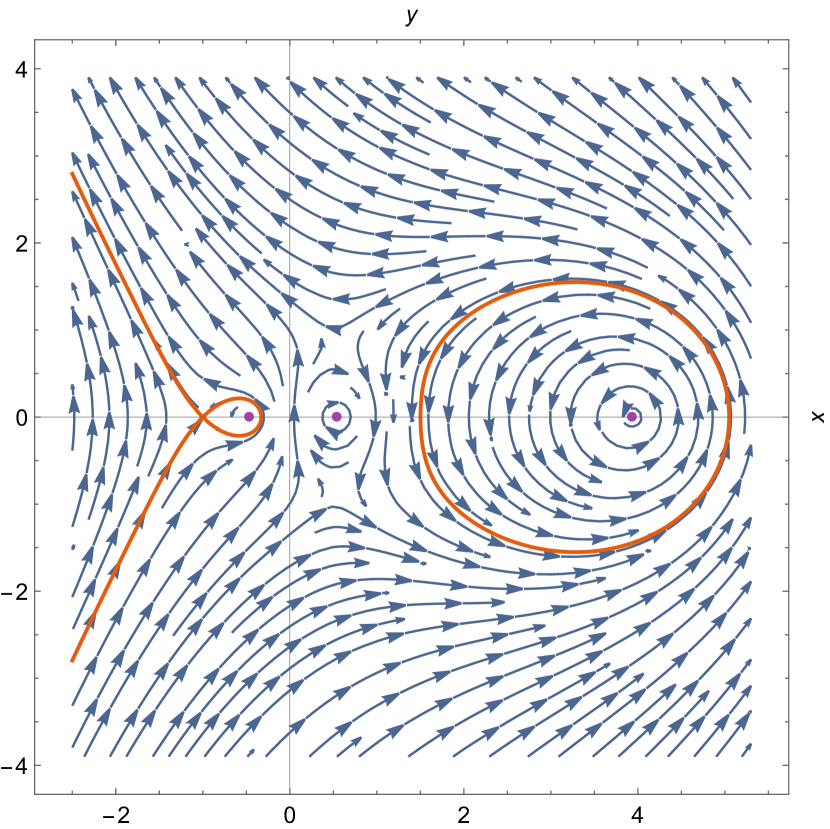
(a) Crossing $-1$.

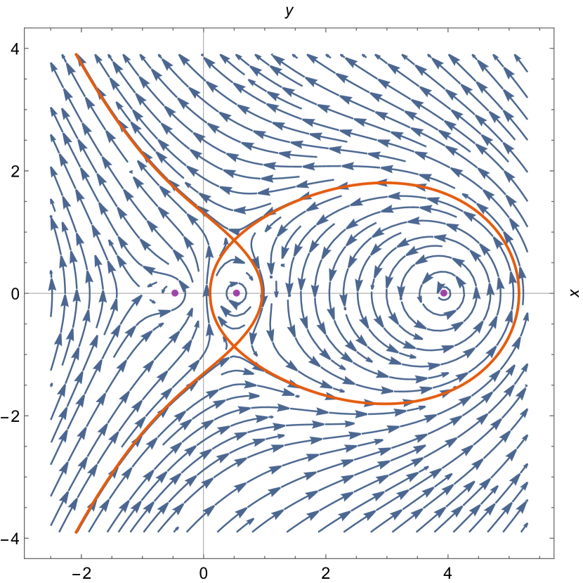
(b) Crossing $(-1)^{1/3}$ and $-(-1)^{2/3}$.

Figure 6: Stokes diagrams for the Hayward BH; $\star\mathrm{d}\real[z(x,y)]$–blue vector fields, and the yellow-brown stream corresponds to the exact Stokes curves, where $M=4$.

Information on the angles at each critical point is shown in Fig. 5, i.e., the angle between two adjacent lines is $\uppi/2$.

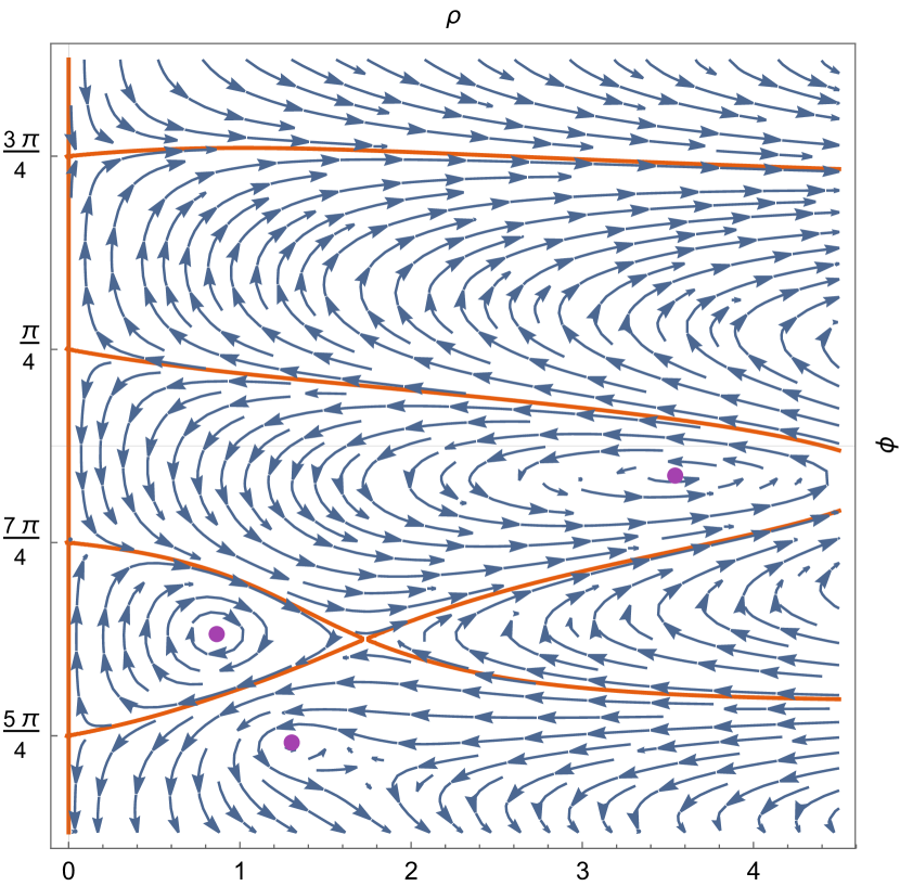
(a) Upper point

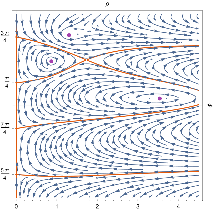
(b) Lower point

Figure 7: Stokes diagrams of the Hayward BH in polar coordinates, with starting points at each critical point.

The tortoise coordinate around $(-1)^{1/3}$ and $-(-1)^{2/3}$ are, respectively,

$$z\sim-\frac{3}{2M}\left[r-(-1)^{1/3}\right]^{2},\quad\text{and}\quad z\sim-\frac{3}{2M}\left[r+(-1)^{2/3}\right]^{2}.$$ (71)

Because $r=0$ is not a point on the Stokes line, we start with the lower critical point $r=(-1)^{1/3}$. The master equation then becomes

$$\left(\frac{\mathrm{d}{}^{2}}{\mathrm{d}z^{2}}+\omega^{2}-\frac{V_{0}}{z^{3/2}}\right)\psi(z)=0,$$ (72)

where $V_{0}=-\sqrt[6]{-1}\sqrt{M}/(2\sqrt{6})$, and its coefficient multivalues owing to $z^{3/2}$. To perform the asymptotic analysis, we apply the perturbation method based on a Bessel-type equation, as mentioned at the end of previous subsection, i.e. we recast the master equation with

$$\left(\frac{\mathrm{d}{}^{2}}{\mathrm{d}z^{2}}+\omega^{2}-\frac{V_{0}}{z^{2+\epsilon}}\right)\psi(\epsilon,z)=0,$$ (73)

and expand the wave function as a power series of $\epsilon$, $\psi(\epsilon,z)=\psi_{0}(z)+\epsilon\psi_{1}(z)+\dots$, where $\epsilon$ is the perturbative parameter. Then, we can obtain the perturbative equations order by order

$$\begin{split}O(\epsilon^{0}),\quad&\psi_{0}^{\prime\prime}(z)+\left(\omega^{2}-\frac{V_{0}}{z^{2}}\right)\psi_{0}(z)=0;\\ O(\epsilon^{1}),\quad&\psi_{1}^{\prime\prime}(z)+\left(\omega^{2}-\frac{V_{0}}{z^{2}}\right)\psi_{1}(z)+\frac{V_{0}\ln(z)}{z^{2}}\psi_{0}(z)=0;\\ \ldots.\quad&\end{split}$$ (74)

Next, to calculate the monodromy, we only use the zero-order equation and drop the order subscript of the wave function to simplify the notation. In other words, our starting point is the solution of the zero-order perturbative equation

$$\psi=B_{1}\sqrt{2\uppi\omega z}J_{\nu/2}(\omega z)+B_{2}\sqrt{2\uppi\omega z}J_{-\nu/2}(\omega z),$$ (75)

where $\nu=\sqrt{1+4V_{0}}$ is a complex number. Moreover, as with the Bardeen BH, we denote the upper and lower critical points as $\mathcal{A}$ and $\mathcal{B}$, respectively, and a point close to the middle horizon as $\mathcal{C}$.

From the lower critical point, we can obtain an asymptotic behavior of the wave function in Eq. (75),

$$\psi_{\mathcal{B}}\sim\left(B_{1}\mathrm{e}^{\mathrm{i}\alpha_{+}}+B_{2}\mathrm{e}^{\mathrm{i}\alpha_{-}}\right)\mathrm{e}^{-\mathrm{i}\omega z},$$ (76)

and the condition

$$B_{1}\mathrm{e}^{-\mathrm{i}\alpha_{+}}+B_{2}\mathrm{e}^{-\mathrm{i}\alpha_{-}}=0,$$ (77)

where $\alpha_{\pm}=\uppi(1\pm\nu)/4$. Then, with the matching $\psi_{\mathcal{\hat{B}}}\leftrightarrow\psi_{\mathcal{C}}$, the asymptotics after rotating around $\mathcal{B}$ with that around $\mathcal{C}$ give another two conditions:

$$\begin{split}B_{1}\mathrm{e}^{3\mathrm{i}\alpha_{+}}+B_{2}\mathrm{e}^{3\mathrm{i}\alpha_{-}}&=C_{1}\mathrm{e}^{-\mathrm{i}\omega\delta+\mathrm{i}\alpha_{+}}+C_{2}\mathrm{e}^{-\mathrm{i}\omega\delta+\mathrm{i}\alpha_{-}},\\ B_{1}\mathrm{e}^{5\mathrm{i}\alpha_{+}}+B_{2}\mathrm{e}^{5\mathrm{i}\alpha_{-}}&=C_{1}\mathrm{e}^{\mathrm{i}\omega\delta-\mathrm{i}\alpha_{+}}+C_{2}\mathrm{e}^{\mathrm{i}\omega\delta-\mathrm{i}\alpha_{-}},\end{split}$$ (78)

where $\delta=\mathrm{i}/(2T_{\rm H}^{-})$, and $T_{\rm H}^{-}$ is the “temperature” of the inner horizon.

With the matching $\psi_{\mathcal{\hat{C}}}\leftrightarrow\psi_{\mathcal{A}}$, the asymptotics of the wave function at $\mathcal{C}$ after rotating around the upper critical point with that at $\mathcal{A}$ provide two more conditions:

$$\begin{split}A_{1}\mathrm{e}^{\mathrm{i}\omega\sqrt{3}+\mathrm{i}\alpha_{+}}+A_{2}\mathrm{e}^{\mathrm{i}\omega\sqrt{3}+\mathrm{i}\alpha_{-}}&=C_{1}\mathrm{e}^{-\mathrm{i}\omega\delta+5\mathrm{i}\alpha_{+}}+C_{2}\mathrm{e}^{-\mathrm{i}\omega\delta+5\mathrm{i}\alpha_{-}},\\ A_{1}\mathrm{e}^{-\mathrm{i}\omega\sqrt{3}-\mathrm{i}\alpha_{+}}+A_{2}\mathrm{e}^{-\mathrm{i}\omega\sqrt{3}-\mathrm{i}\alpha_{-}}&=C_{1}\mathrm{e}^{\mathrm{i}\omega\delta+3\mathrm{i}\alpha_{+}}+C_{2}\mathrm{e}^{\mathrm{i}\omega\delta+3\mathrm{i}\alpha_{-}}.\end{split}$$ (79)

where $\sqrt{3}$ originates from a shift in the variable in Eq. (75) from the lower critical point to the upper, i.e. $z\to z+\sqrt{3}$, because the difference between the upper critical point and the lower is $\imaginary\left[(-1)^{1/3}\right]-\imaginary\left[-(-1)^{2/3}\right]=\sqrt{3}$.

Finally, after closing the contour and comparing it with the change around the outer horizon, we arrive at

$$\frac{A_{1}\mathrm{e}^{\mathrm{i}\omega\sqrt{3}-\mathrm{i}\alpha_{+}}+A_{2}\mathrm{e}^{\mathrm{i}\omega\sqrt{3}-\mathrm{i}\alpha_{-}}}{B_{1}\mathrm{e}^{\mathrm{i}\alpha_{+}}+B_{2}\mathrm{e}^{\mathrm{i}\alpha_{-}}}=\mathrm{e}^{\frac{\omega}{T_{\rm H}^{+}}},$$ (80)

where $T_{\rm H}^{+}$ denotes the temperature of the outer horizon. Furthermore, combining all the above conditions, we obtain an analytical expression for the AQMNs,

$$\mathrm{e}^{\omega/T^{+}_{\rm H}}=-2\mathrm{e}^{-\omega/T^{-}_{\rm H}}[\cos(\uppi\nu)+1]-2\cos(\uppi\nu)-1,$$ (81)

which has a similar form to the result in Ref. [32] because the track along the Stokes lines is similar to that of RN BH. However, there is an essential difference, in our result, the AQNMs should not depend on the multipole number $l$ because $r=0$ is not a singular point of the Stokes lines, and thus rotation of the asymptotic solution around $r=0$ is trivial, and $l$ does not appear in the formula of AQNMs.

4.3 Universal form of asymptotic quasinormal modes

For the third class of RBHs generalized by the nonlinear electrodynamic source in Ref. [17], we simply choose $\mu=3$, yielding the matter Lagrangian [17]

$$\mathcal{L}=\frac{12}{\alpha}\frac{\alpha\mathcal{F}}{(1+(\alpha\mathcal{F})^{1/4})^{4}},\qquad\alpha=P^{3}/M$$ (82)

and the shape function

$$f=1-\frac{2Mr^{2}}{(P+r)^{3}},$$ (83)

and use the transformation $r\to Pr$ and $M\to MP/2$ to rescale the variables, such that all the parameters appearing in the shape function are dimensionless. Furthermore, there is one critical point $r=-1$ and three horizons in this model, see Fig. 8, and from the critical point, there are eight Stokes lines emitting with adjacent angle of $\uppi/4$.

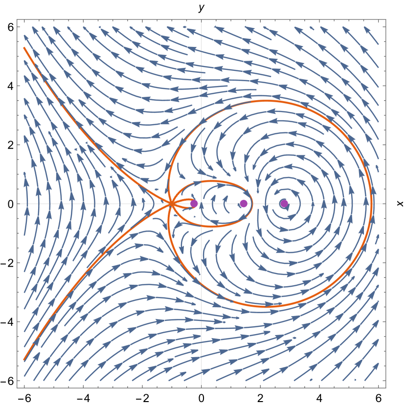
(a) Cartesian coordinates

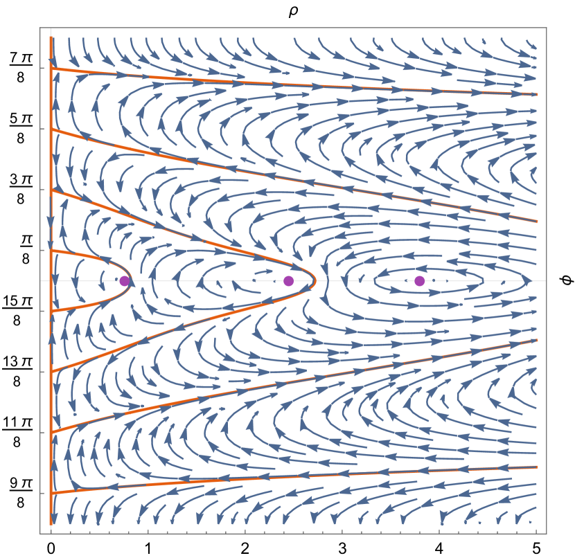
(b) Polar coordinates starting at $r=-1$

Figure 8: Stokes diagrams for the third class of RBHs; $\star\mathrm{d}\real[F(x,y)]$–blue vector fields, and the yellow-brown curves correspond to the Stokes lines, where $M=7$.

Approaching the critical point, the leading term of the tortoise coordinate is

$$r_{*}\sim-\frac{(r+1)^{4}}{4M},$$ (84)

and thus the master equation becomes

$$\left(\frac{\mathrm{d}{}^{2}}{\mathrm{d}z^{2}}+\omega^{2}-\frac{V_{0}}{z^{7/4}}\right)\psi(z)=0,$$ (85)

where $V_{0}=3\sqrt[4]{-M}/(8\sqrt{2})$. The same as before, we apply perturbation theory and take the zero-order solution as the asymptotics of the master equation at the critical point. This procedure gives us a similar Bessel-type function.

On the other side, the closed contour starts from the bottom left of Fig. 8(a), and approaches the critical point before rotating $\uppi/2$ in $r$ (i.e., $2\uppi$ in $z$). Subsequently, it moves toward the middle horizon, returns to the critical point, and then finally reaches the top left corner by rotating $\uppi/2$ in $r$.

The expression for the AQNMs of this third class is formally the same as that of the Hayward BH, Eq. (81), but with a different value of $\nu$. This implies that the matching of $\psi_{\mathcal{\hat{C}}}\leftrightarrow\psi_{\mathcal{A}}$ in the case of the Hayward BH can be ignored. Moreover, this reflects the fact that a transformation, such as Eq. (69), should not affect the physical results, even though the numerical values of the upper and lower critical points depend on the scale transformations.

From the above examples, we clearly see that the AQNMs have the same form as long as the traces of the asymptotic solutions along the Stokes lines are similar. Let us analyze one more integrable example.

Inspired by [59], we construct the following shape function:

$$f=\left(1-\frac{P^{2}}{r^{2}}\right)^{2}\left(\sqrt{1-\frac{P^{2}}{r^{2}}}-\frac{2M}{r}\right),$$ (86)

where $P$ is interpreted as magnetic charge, as before. The complete roots of $f(r)=0$ include $\pm P$ and $\pm\sqrt{P^{2}+4M^{2}}$, among which only the positive are physical. The AQNMs of a similar type of RBH have been considered in Refs. [60, 61].

The physical radius of this BH cannot be less than $P$, otherwise the metric becomes complex. Even though the curvature invariants are mathematically divergent at the zero point, the physical condition $r\geq P$ forbids any test particle from passing into the inner horizon $r_{-}=P$. Therefore, all the curvature invariants are finite in the physical domain $r\in[P,\infty)$. Moreover, the origin is the only critical point, and the tortoise coordinate can be obtained analytically,

$$2(z+z_{0})=\frac{2r^{2}}{\sqrt{r^{2}-1}}+\frac{1}{r^{2}-1}+\ln\left[\frac{\left(2-r^{2}\right)^{8}}{\left(1-r^{2}\right)^{3}\left(r^{2}+2\sqrt{r^{2}-1}\right)^{4}}\right],$$ (87)

where $z_{0}=-1/2+\ln(4)+\mathrm{i}\uppi$, and we use the normalization $r\to 2Mr$ and $P\to 2MP$ and set $P=1$. Thus

$$z\sim-\left(1+\mathrm{i}\right)r^{6}/12$$ (88)

which implies that there are twelve Stokes lines emitting from the origin, and the angle between any two adjacent lines is $\uppi/6$, see Fig. 9.

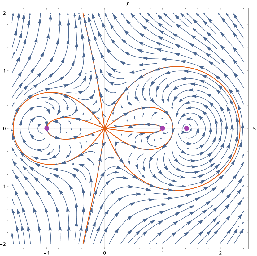
(a) Cartesian coordinates

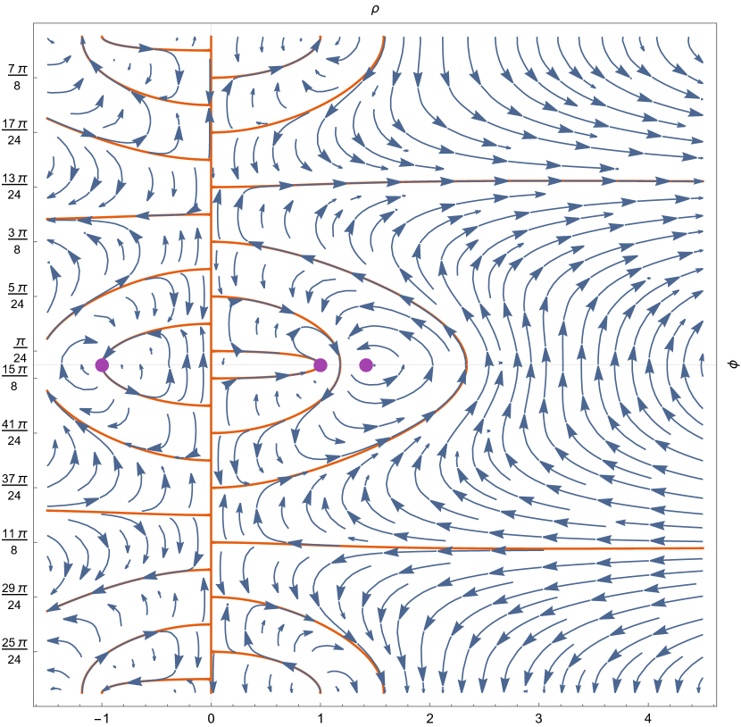
(b) Polar coordinates

Figure 9: Stokes diagrams for the PK BH; $\star\mathrm{d}\real[F(x,y)]$–blue vector fields, and the yellow-brown curves correspond to the Stokes lines, where $M=1/2$ and $P=1$.

The master equation is

$$\psi^{\prime\prime}(z)+\left(\omega^{2}-\frac{5}{36z^{2}}\right)\psi(z)=0.$$ (89)

Thus, the monodromy relation is similar to that for the RN BH,

$$\mathrm{e}^{\omega/T^{+}_{\rm H}}=-\left[1+2\cos(\uppi\nu)\right]-2\left[1+\cos(\uppi\nu)\right]\mathrm{e}^{-\omega/T^{-}_{\rm H}},$$ (90)

where $\nu=\sqrt{14}/3$. Substituting the explicit forms of the temperatures of the inner and outer horizons,

$$T^{+}_{\rm H}=\frac{2M^{3}}{\uppi\left(4M^{2}+P^{2}\right)^{2}},\qquad T^{-}_{\rm H}=0,$$ (91)

we arrive at

$$\omega/T^{+}_{\rm H}=2\mathrm{i}\uppi n+\ln\left[-1-2\cos\left(\uppi\sqrt{14}/3\right)\right].$$ (92)

As a step summary, we have shown that the analytical form of AQNMs may be universal if the trajectories of the asymptotic solutions along the Stokes lines are similar; however, they should not depend on the multipole number $l$.

5 Regular black holes with essential singularities or without singularities

The models considered in Sec. 3 have a common aspect: the singularities of RBHs still exist (defined as the second types), but they are simply moved to the classically forbidden region. In the current section, we investigate several exotic examples that belong to the first and third types discussed in Sec. 2.

5.1 Essential singularity as a semi-critical point

Let us express the shape function with an essential singularity at $r=0$ as [62, 21]

$$f(r)=1-\frac{2M}{r}\sigma(r),\qquad\sigma(r)=\mathrm{e}^{-\frac{P^{2}}{2Mr}},$$ (93)

where $P$ is interpreted as magnetic charge. The Lagrangian of the matter source as a nonlinear magnetic monopole can be found as

$$\mathcal{L}=\frac{4P^{3}}{\mathcal{F}}\exp\left[-\frac{P^{9/4}}{2^{3/4}M\sqrt[4]{\mathcal{F}}}\right].$$ (94)

To perform an appropriate analysis, we use a dimensionless representation with the help of the rescaling transformation [28]

$$r\to\frac{2M}{P^{2}}r,\qquad P\to\frac{2M}{P}.$$ (95)

The shape function then becomes

$$f(r)=1-\frac{P^{2}}{r}\mathrm{e}^{-1/r}.$$ (96)

When $r\in\mathbb{R}$, there are two real horizons $r_{\rm H}=-1/W_{n}\left(-P^{-2}\right)$ with $n=0,-1$ if $P^{2}>\mathrm{e}$. Here $W_{n}(z)$ is the Lambert W function [63]. When $r$ is analytically continued into the complex plane, $n$ is enlarged to all natural numbers $\mathbb{N}$, i.e., the roots of $f(r_{\rm H})=0$ are infinitely many according to Picard’s great theorem [51] because $r=0$ is an essential singularity of $f(r)$. Meanwhile, all of these roots except the physical horizons are bounded by $\absolutevalue{r_{\rm H}}\leq\absolutevalue{-1/W_{0}\left(-P^{-2}\right)}$ and located symmetrically with respect to the real axis because $W^{*}_{n}\left(-P^{-2}\right)=W_{-n-1}\left(-P^{-2}\right)$ if $n\neq 0,-1$.

To find the critical points, it is equivalent to calculate the zeros of $r\mathrm{e}^{1/r}$ because

$$1/f=\frac{r\mathrm{e}^{1/r}}{r\mathrm{e}^{1/r}-P^{2}},$$ (97)

but $r\mathrm{e}^{1/r}$ does not have any zeros on the complex plane, i.e, the zero is a Picard exceptional value of $1/f$. Thus, there are no critical points for this model. However, the origin $r=0$ is a jump discontinuity,

$$\lim_{r\to 0^{+}}1/f=1,\qquad\lim_{r\to 0^{-}}1/f=0,$$ (98)

which signifies that it may play a special role in the Stokes diagram, even though it is not a critical point. The superscript in $0^{+}$ ($0^{-}$) indicates that the path of the limit to $0$ is taken in the right (left) half-plane. From the perspective of the Weyl curvature

$$W=\frac{P^{12}}{48M^{4}}\frac{\mathrm{e}^{-2/r}}{r^{10}}[6(r-1)r+1]^{2},$$ (99)

the jump discontinuity of $r=0$ implies that

$$\lim_{r\to 0^{+}}W=0,\qquad\lim_{r\to 0^{-}}W\to\infty,$$ (100)

i.e., the Weyl curvature is divergent at the essential singularity $r=0$ as $r$ approaches zero from the left half-plane. Thus, we dub $r=0$ as the semi-critical point because it is different from regular points and the critical points considered in Sec. 3.

To perform a quantitative analysis of the Stokes lines, we apply the asymptotic relation $1/f(r)\sim-r\mathrm{e}^{1/r}/P^{2}$ as $r\to 0^{-}$ and rewrite Eq. (21) as

$$z^{\prime}(r) \approx-\frac{r}{P^{2}}\mathrm{e}^{1/r}\quad\text{with}\quad z(0^{-})=0,$$ (101)

which provides the solution

$$z(r) =-\frac{1}{2P^{2}}\mathrm{e}^{1/r}r(r+1)+\frac{1}{2P^{2}}{\rm Ei}\left(\frac{1}{r}\right)\sim\frac{\mathrm{e}^{1/r}r^{3}}{P^{2}}$$ (102)

where ${\rm Ei}$ denotes the exponential integral [63]. Thus, the Stokes lines $\real[z]=0$ around $0^{-}$ are approximately

$$y\left(3x^{2}-y^{2}\right)\sin\left(\frac{y}{x^{2}+y^{2}}\right)+x\left(x^{2}-3y^{2}\right)\cos\left(\frac{y}{x^{2}+y^{2}}\right)=0.$$ (103)

Along the longitudinal direction, $x=0$, this reduces to

$$0=y^{3}\sin\left(\frac{1}{y}\right).$$ (104)

As a results, we find that there are infinite Stokes lines quantified by $1/y=n\uppi$ with $n\in\mathbb{Z}/\{0\}$ owing to the periodicity of the sine function, see Fig. 10.

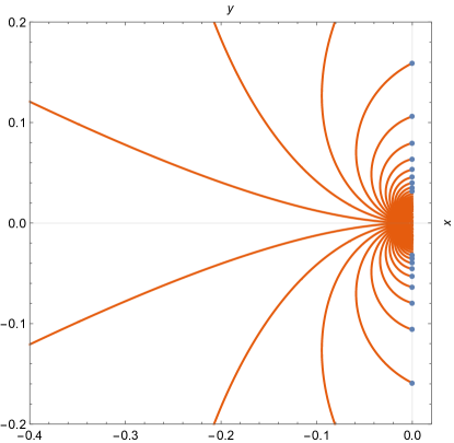
Figure 10: Stokes diagrams in Cartesian coordinates for the Balart–Vagenas BH close to $0^{-}$. The yellow-brown curves are Stokes lines, whereas the blue points are their intersections with the longitudinal axis $y$.

This phenomenon of infinitely many Stokes lines around the essential singularity $r=0$ is also a reflection of Picard’s great theorem.

To fix the angle between two adjacent Stokes lines at $0^{-}$, we rewrite Eq. (103) in the polar system $\{\rho,\phi\}$, which gives

$$\rho\cos\left[3\phi-\frac{\sin(\phi)}{\rho}\right]=0.$$ (105)

When $\rho$ becomes small, we find that

$$\sin(\phi)\approx\frac{2n+1}{2}\uppi\rho\to 0.$$ (106)

That is, $\phi=\uppi$ as $r\to 0^{-}$. In other words, the angles of all Stokes lines emitting from $0^{-}$ are zero. see Fig. 11.

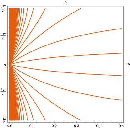
Figure 11: Stokes diagrams in polar coordinates for the Balart–Vagenas BH close to $0^{-}$.

The full Stokes lines are computed using a numeric integral and are depicted in Fig.12.

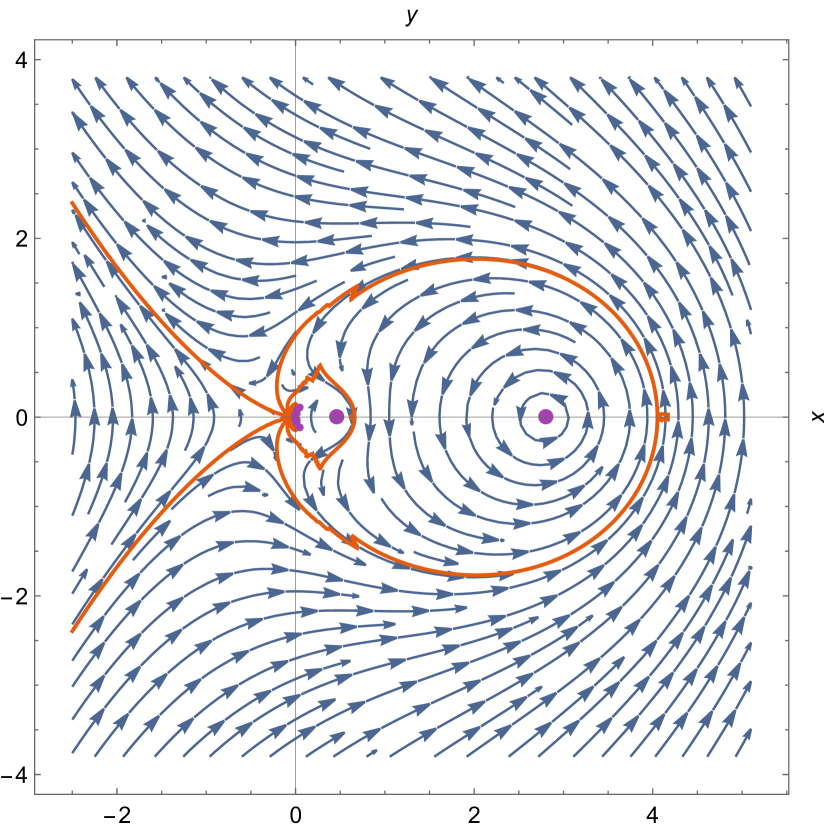
(a) Cartesian coordinates

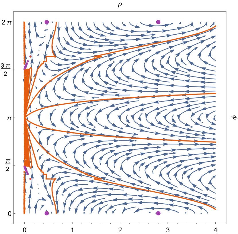
(b) Polar coordinates

Figure 12: Stokes diagrams for the Balart–Vagenas BH; $\star\mathrm{d}\real[z(x,y)]$–blue vector fields, and the yellow-brown curves correspond to the Stokes lines, where $P=2$.

Because of the extreme characteristic of the integrand near the singularities, the lines are not smooth at all, as shown in the plot. Alternatively, we develop a formula based on the Cauchy–Riemann equations [51] to estimate the global feature of Stokes lines in the range far from the origin,

$$0=\int^{x}_{0}\mathrm{d}\widetilde{x}\real\left[\frac{1}{f(\widetilde{x}+\mathrm{i}y)}\right]-\int^{y}_{0}\mathrm{d}\widetilde{y}\lim_{x\to 0}\imaginary\left[\frac{1}{f(x+\mathrm{i}\widetilde{y})}\right],$$ (107)

which loses its validity as $x\to 0^{-}$ because an infinite number of complex horizons are located there, see Fig. 13.

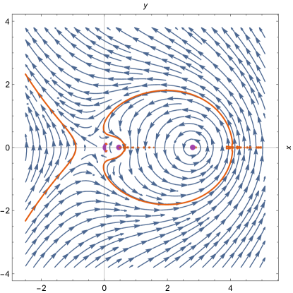
Figure 13: Improved Stokes lines for the Balart–Vagenas BH based on the numeric integral in Eq. (107) with $P=2$.

Now we turn to the master equation. First, we obtain the asymptotic form of the potential in Eq. (18) as $r\to 0^{-}$

$$V\sim\frac{P^{4}\mathrm{e}^{-2/r}}{r^{5}},$$ (108)

and then with the help of the asymptotic relation in Eq. (102), we can rewrite the master equation as

$$\left[\frac{\mathrm{d}{}^{2}}{\mathrm{d}z^{2}}+\omega^{2}+\frac{1}{3z^{2}W_{0}\left(\frac{1}{3P^{2/3}\sqrt[3]{-z}}\right)}\right]\psi(z)=0,$$ (109)

However, because the angles of the Stokes lines emitting from the origin are zero, a trivial monodromy relation is obtained, i.e. $1=\exp(\omega/T^{+}_{\rm H})$, which gives a pure imaginary spectrum of the AQNMs, $\omega=2\uppi\mathrm{i}nT^{+}_{\rm H}$.

5.2 No critical points at all

Next we turn to a RBH model inspired by noncommutative geometry [64],

$$f(r)=1-\frac{2M}{r}\sigma,\qquad\sigma(r)=\frac{2}{\sqrt{\uppi}}\gamma\left(\frac{3}{2},\frac{r^{2}}{4\epsilon}\right),$$ (110)

where $\epsilon$ denotes the noncommutative parameter, and $\gamma\left(\frac{3}{2},\frac{r^{2}}{4\epsilon}\right)$ is the lower incomplete gamma function [63]. The original model was proposed by considering the existence of a minimum distance scale. However, we use the monopole interpretation instead of the original model, i.e., we replace the parameter $\epsilon$ with $P^{2}$. Thus, the Lagrangian can be obtained as

$$\mathcal{L}=\frac{2M}{P^{3}\sqrt{\uppi}}\mathrm{e}^{-\frac{\sqrt{\mathcal{F}}}{4\sqrt{2}P^{5/2}}}.$$ (111)

Then, with the help of the following transformation [28];

$$r\to\frac{2PM}{\sqrt{\uppi}}r,\qquad P\to\frac{PM}{\sqrt{\uppi}},$$ (112)

the shape function becomes

$$f=1-\frac{2}{Pr}\gamma\left(\frac{3}{2},r^{2}\right),$$ (113)

where the parameter $P$ is bounded by $0.93\gtrsim P>0$, otherwise there will be not physical horizons.

The complex extended horizons can be calculated numerically using $f(r)=0$. The distribution of complex horizons depends on the value of $\absolutevalue{r}$, which can be illustrated by the argument principle, see Fig. 14, where we show winding indices for the images of circles with different moduli $\absolutevalue{r}$.

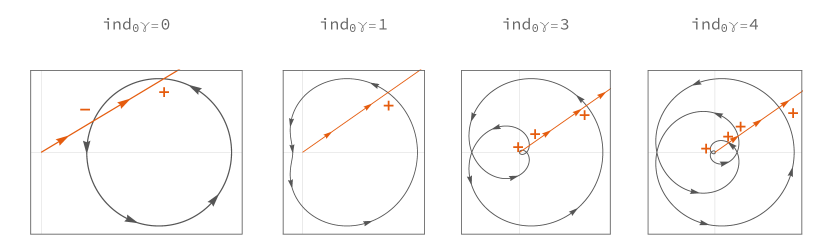
Figure 14: Winding indices. The images (black closed curves) of circles with radii $\absolutevalue{r}=1/2,1,3,4$ from left to right under the map of Eq. (113), where $P=1/2$. The yellow-brown rays from zero to infinity are auxiliary lines for calculating the winding indices. The signs “$\pm$” correspond to the counter-clockwise and clockwise intersections of the curve with the ray, respectively.

The number of complex horizons increases with increasing modulus $\absolutevalue{r}$. Moreover, we can find a property of the horizons, that is, if $r$ is a horizon, its conjugate $r^{*}$ is also a horizon because $\gamma^{*}(3/2,z^{2})=\gamma(3/2,(z^{*})^{2})$, and thus, $0=f^{*}(r)=f(r^{*})$, see Fig. 15(a).

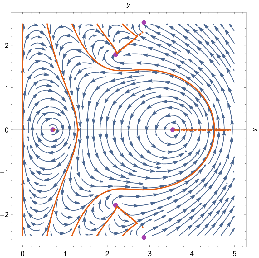
(a) Cartesian coordinates

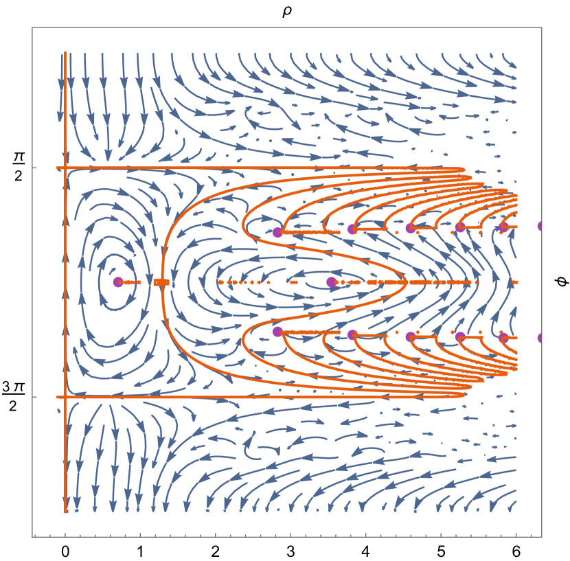
(b) Polar coordinates

Figure 15: Stokes diagrams for the Eq. (110) BH; $\star\mathrm{d}\real[F(x,y)]$–blue vector fields with $P=1/2$.

As the modulus of $r=x+\mathrm{i}y$ becomes large, the complex horizons can be approximately computed by solving the system

$$4\mathrm{e}^{y^{2}-x^{2}}\cos(2xy)+1=0,\qquad\sin(2xy)=0$$ (114)

which gives

$$2xy=2\uppi n+\uppi,\qquad x^{2}-y^{2}=2\ln(2)$$ (115)

with $n\in\mathbb{Z}$. We can also verify that there are neither critical nor semi-critical points in this model, because $\gamma\left(3/2,r^{2}\right)/r$ is an entire function. In particular, $1/f$ approaches $1$ as $r\to 0$. Therefore, the monodromy of the asymptotic solutions along any closed curve is trivial, which leads to a similar result to that of the above example, $1=\exp(\omega/T^{+}_{\rm H})$.

However, if we consider the small-charge approximation $P\sim 0$, i.e., if we treat the RBH model as a singular one, we obtain

$$f(r)\sim 1-\frac{\sqrt{\uppi}}{Pr}+\frac{2}{P}\mathrm{e}^{-r^{2}},$$ (116)

which has a critical point at zero and one real horizon. In other words, the Stokes diagram of this model in the small-charge approximation is similar that of the Schwarzschild BH. The tortoise coordinate and effective potential close to zero are, respectively,

$$z\sim-\frac{r^{2}}{4\sqrt{\uppi}},\qquad V\sim-\frac{\uppi}{P^{2}r^{4}}.$$ (117)

The master equation becomes

$$\left(\frac{\mathrm{d}{}^{2}}{\mathrm{d}z^{2}}+\omega^{2}-\frac{1}{16P^{2}z^{2}}\right)\psi(z)=0,$$ (118)

and the monodromy relation is then

$$-\left[1+2\cos(\uppi\nu)\right]=\mathrm{e}^{\omega/T_{\rm H}}$$ (119)

with

$$\nu=\frac{1}{2}\sqrt{\frac{1}{P^{2}}+4},\qquad T_{\rm H}=\frac{\sqrt{\uppi}\mathrm{e}^{r_{\rm H}^{2}}-4r_{\rm H}^{3}}{4\uppi^{3/2}\mathrm{e}^{r_{\rm H}^{2}}r_{\rm H}-8\uppi r_{\rm H}^{2}}.$$ (120)

As we find in this section, the analytical spectrum of the AQNMs reduces to an extreme simple form because the monodromy of the asymptotic solutions along any closed Stokes lines is trivial.

6 Relationship between the monodromy method and WKB approach

To study the AQNMs using the complex WKB approach, Andersson and Howls used another method to diagonalize the differential operator in the master equation, where the radial coordinate, unlike the tortoise coordinate, is no longer mutivalued [65]. The diagonalized master equation in Andersson and Howls’ approach is

$$\frac{\mathrm{d}^{2}\Phi}{\mathrm{d}r^{2}}+Q^{2}\Phi=0$$ (121)

with

$$Q^{2}=f^{-2}Q^{2}_{0},\qquad Q^{2}_{0}=\left[\omega^{2}-V(r)+\frac{1}{4}\left(\frac{\mathrm{d}f}{\mathrm{d}r}\right)^{2}-\frac{1}{2}f\left(\frac{\mathrm{d}^{2}f}{\mathrm{d}r^{2}}\right)\right]$$ (122)

where $V(r)$ is the same as in Eq. (18), and $\Phi$ connects with $\psi$ via $\Phi=f^{1/2}\psi$. The Stokes lines are defined by

$$\imaginary\left[\int^{r}_{r_{0}}Q(r^{\prime})\mathrm{d}r^{\prime}\right]=0.$$ (123)

Generally, the integral in Eq. (123) cannot be calculated analytically for RBHs. Therefore, we use the WKB Stokes field $\{\real[Q],-\imaginary[Q]\}$ to depict the Stokes portrait, see Fig. 16, where the Stokes field for Schwarzschild and RN BHs are shown.

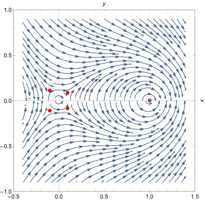
(a) Schwarzschild BH

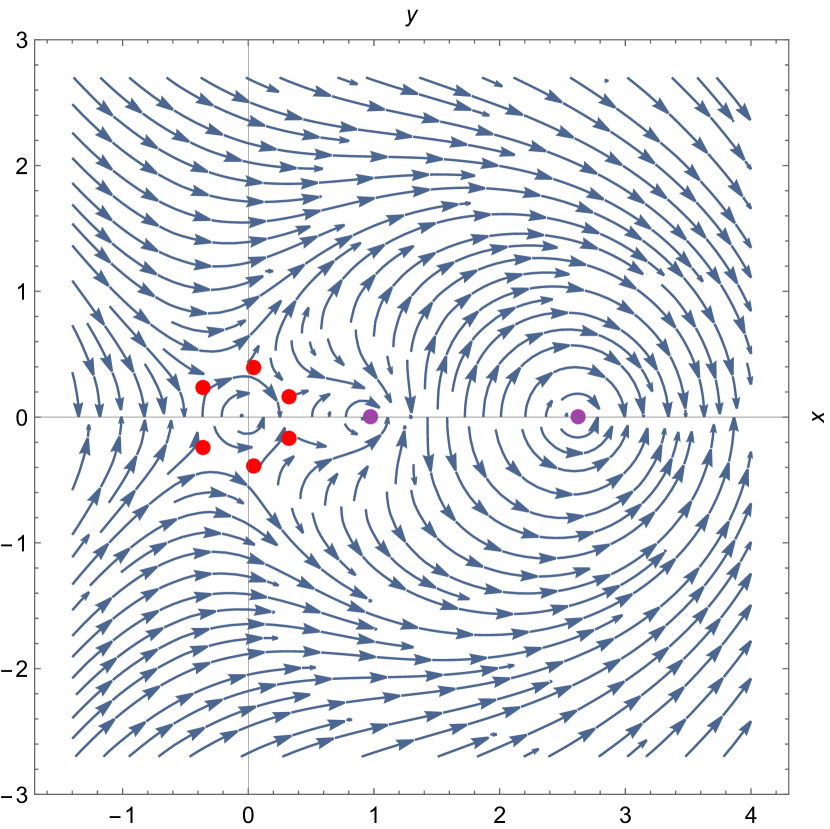
(b) Reissner–Nordström BH

Figure 16: Stokes field $\{\real[Q],-\imaginary[Q]\}$. The purple points denote horizons, whereas the red points are zeros of $Q$.

We use the term “WKB Stokes field” to distinguish it from the one we discuss in the monodromy method. However, for a given BH model, these two fields are related. To see it clearly, let us take the damping limit $\omega\to-\mathrm{i}\infty$ in the WKB Stokes field, which gives us $Q\sim-\mathrm{i}\absolutevalue{\imaginary(\omega)}/f(r)$ for $r\geq r_{\rm H}$. Thus, the WKB Stokes field in the damping limit becomes

$$\{\real[Q],-\imaginary[Q]\}\sim\absolutevalue{\imaginary(\omega)}\left\{\imaginary\left[1/f(r)\right],\real\left[1/f(r)\right]\right\}$$ (124)

which is the scaled Stokes field in the monodromy method, Eq. (28). Furthermore, for singular BHs, the critical points (zeros) of $Q$ converge to the origin (essential singularities) of BHs as $\imaginary(\omega)\to\infty$, and the WKB Stokes field becomes the Stokes field in the monodromy method.

The situation for RBHs is slightly different from the above case for singular BHs. $Q_{0}^{2}$ of RBHs has two zeros around the origin $r=0$ owing to $V\sim r^{-2}$ (see Fig. 17), even though $r=0$ is not a zero of $f^{-2}$. However, these two zeros do not converge to the origin but disappear as $\omega\to-\mathrm{i}\infty$ because $\omega$ dominates in $Q_{0}^{2}$ at that moment. As a result, $r=0$ becomes a regular point in the damping limit. In other words, the AQNMs via the complex WKB approach, like in the monodromy method, are not dependent on the behavior around the BH center.

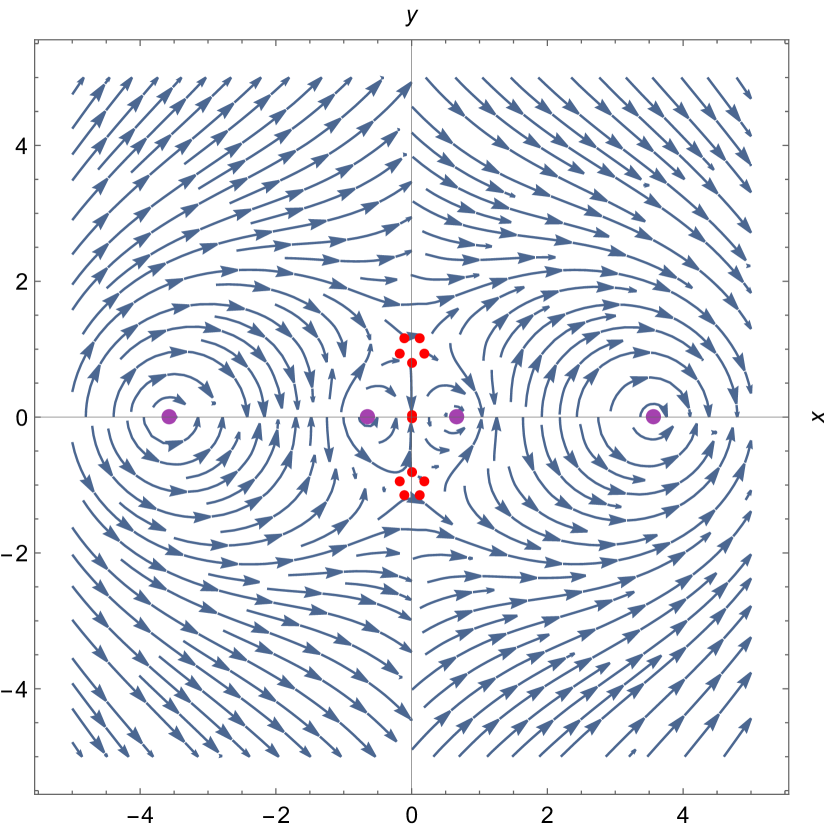
(a) Bardeen BH

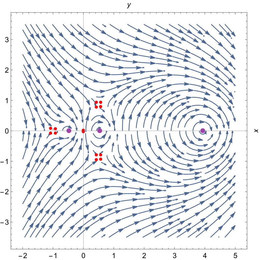
(b) Hayward BH

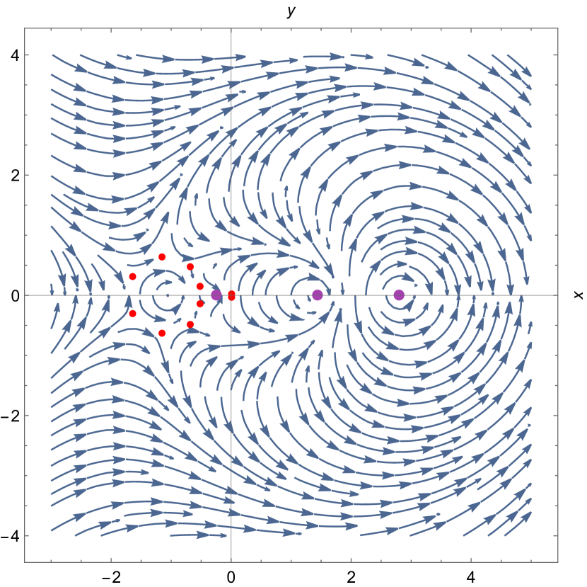
(c) Third class BH

Figure 17: Stokes field $\{\real[Q],-\imaginary[Q]\}$. The purple points denote horizons, whereas the red points are zeros of $Q$.

7 Conclusions and outlook

In this study, to calculate the AQNMs of RBHs, we apply the Stokes field to extensively investigate the local characteristics of the Stokes lines and classify RBHs based on the types of their complex singularities, which arise as a result of the analytical continuation of the radial coordinate into the complex plane.

From the calculation, we find several novel aspects of the AQNMs of RBHs, i.e., the analytical forms of the asymptotic frequency spectrum are not universal for spherically symmetric RBHs with single shape functions and do not depend on the multipole number $l$ because $r=0$ is not a point on the Stokes lines; even if $r=0$ is a point on the Stokes lines, it must not be an accumulation point, such that the rotation of the asymptotic solution around $r=0$ is trivial and $l$ does not appear in the formula of the AQNM.

The forms of asymptotic frequency may depend on the structures of the Stokes portraits.

1. The existence of singularities. The absence of singularities leads to a trivial monodromy, such that the asymptotic frequency is purely imaginary.

2. The rotation angle of the asymptotic solutions around singularities. If the rotation angle is trivial, the asymptotic frequency also has only the imaginary part.

3. The trajectory of the asymptotic solutions along the Stokes lines. It is not the topology of the Stokes line that plays a decisive role, but the way of bypassing the trajectory.

In a broader sense, specific research on AQNMs relates to several mathematical topics, such as transcendental curves and the value distribution of holomorphic functions. As shown in this study, even the simplest Stokes lines obtained from the Schwarzschild BH cannot be depicted by a polynomial, whereas the Stokes lines for RBHs are usually not integrable and have no analytical expressions.

On the one hand, to provide aspects of the Stokes lines, we attempt several numerical methods in this study to remove the integral of the tortoise coordinate, e.g., Newton–Cotes quadrature rules. Nevertheless, the results obtained from these numerical methods more or less lose some important information on the Stokes lines.

On the other hand, the situation of the complex singularities (curvature and coordinate singularities) of RBHs becomes intricate because the Stokes lines must have self-intersections at curvature singularities, and their closed parts must surround the coordinate singularities. Thus, the distribution of the zeros and poles of the shape functions directly affect the appearance of the Stokes lines. Clarification of the value distribution may help us construct information on the Stokes lines. Therefore, we will devote ourselves to developing more effective approaches to obtaning the feature of Stokes lines in future studies.

Finally, because our main motivation for studying the AQNMs is to obtain the quantum entropy spectrum of RBHs, our subsequent work will focus on how to derive the correct quantum entropy spectrum based on the AQNMs obtained in this study.

References

- [1] E. Ayon-Beato and A. Garcia, “Regular black hole in general relativity coupled to nonlinear electrodynamics,” Phys. Rev. Lett. 80 (1998) 5056–5059, arXiv:gr-qc/9911046.
- [2] S. A. Hayward, “Formation and evaporation of nonsingular black holes,” Phys. Rev. Lett. 96 (Jan., 2006) 031103, arXiv:gr-qc/0506126 [gr-qc].
- [3] S. Ansoldi, “Spherical black holes with regular center: A Review of existing models including a recent realization with Gaussian sources,” in Conference on Black Holes and Naked Singularities. 2, 2008. arXiv:0802.0330 [gr-qc].
- [4] M. A. Markov, “Limiting density of matter as a universal law of nature,” JETP Lett. (Engl. Transl.); (United States) 36 (9, 1982) 214–216. https://www.osti.gov/biblio/6268156.
- [5] V. P. Frolov, “Notes on nonsingular models of black holes,” Phys. Rev. D 94 no. 10, (2016) 104056, arXiv:1609.01758 [gr-qc].
- [6] S. W. Hawking and G. F. R. Ellis, The Large Scale Structure of Space-Time. Cambridge Monographs on Mathematical Physics. Cambridge University Press, 2, 2011.
- [7] R. M. Wald, General Relativity. University of Chicago Press, Chicago, USA, 1984.
- [8] C. W. Misner and A. H. Taub, “A Singularity-free Empty Universe,” Sov. Phys. JETP 28 (1969) 122. http://www.jetp.ras.ru/cgi-bin/dn/e_028_01_0122.pdf.
- [9] V. Kagramanova, J. Kunz, E. Hackmann, and C. Lammerzahl, “Analytic treatment of complete and incomplete geodesics in Taub-NUT space-times,” Phys. Rev. D 81 (2010) 124044, arXiv:1002.4342 [gr-qc].
- [10] G. J. Olmo, D. Rubiera-Garcia, and A. Sanchez-Puente, “Geodesic completeness in a wormhole spacetime with horizons,” Phys. Rev. D 92 no. 4, (2015) 044047, arXiv:1508.03272 [hep-th].
- [11] A. D. Sakharov, “The initial stage of an expanding Universe and the appearance of a nonuniform distribution of matter,” Sov. Phys. JETP 22 (1966) 241.
- [12] E. B. Gliner, “Algebraic Properties of the Energy-momentum Tensor and Vacuum-like States of Matter,” Sov. Phys. JETP 22 (1966) 378.
- [13] A. Borde, “Regular black holes and topology change,” Phys. Rev. D 55 (1997) 7615–7617, arXiv:gr-qc/9612057.
- [14] I. Dymnikova, “Vacuum nonsingular black hole,” Gen. Rel. Grav. 24 (1992) 235–242.
- [15] J. M. Bardeen, “Non-singular general-relativistic gravitational collapse,” in Conference Proceedings of GR5, Tbilisi, USSR, vol. 174. 1968.
- [16] E. Ayon-Beato and A. Garcia, “The Bardeen model as a nonlinear magnetic monopole,” Phys. Lett. B 493 (2000) 149–152, arXiv:gr-qc/0009077.
- [17] Z.-Y. Fan and X. Wang, “Construction of regular black holes in general relativity,” Phys. Rev. D 94 (Dec., 2016) 124027, arXiv:1610.02636 [gr-qc].
- [18] E. Ayon-Beato and A. Garcia, “Four parametric regular black hole solution,” Gen. Rel. Grav. 37 (2005) 635, arXiv:hep-th/0403229.
- [19] P. Nicolini, “Noncommutative Black Holes, The Final Appeal To Quantum Gravity: A Review,” Int. J. Mod. Phys. A 24 (2009) 1229–1308, arXiv:0807.1939 [hep-th].
- [20] C. Bambi and L. Modesto, “Rotating regular black holes,” Phys. Lett. B 721 (2013) 329–334, arXiv:1302.6075 [gr-qc].
- [21] L. Balart and E. C. Vagenas, “Regular black holes with a nonlinear electrodynamics source,” Phys. Rev. D 90 (Dec., 2014) 124045, arXiv:1408.0306 [gr-qc].
- [22] C. Lan, Y.-G. Miao, and Y.-X. Zang, “Acoustic regular black hole in fluid and its similarity and diversity to a conformally related black hole,” Eur. Phys. J. C 82 no. 3, (2022) 231, arXiv:2109.13556 [gr-qc].
- [23] C. Lan, Y.-G. Miao, and Y.-X. Zang, “Simulations of physical regular black holes in fluids,” arXiv:2206.08694 [gr-qc].
- [24] A. Bonanno and M. Reuter, “Renormalization group improved black hole space-times,” Phys. Rev. D 62 (2000) 043008, arXiv:hep-th/0002196.
- [25] K. A. Bronnikov and J. C. Fabris, “Regular phantom black holes,” Phys. Rev. Lett. 96 (2006) 251101, arXiv:gr-qc/0511109.
- [26] L. Modesto, “Super-renormalizable Quantum Gravity,” Phys. Rev. D 86 (2012) 044005, arXiv:1107.2403 [hep-th].
- [27] L. Modesto, J. W. Moffat, and P. Nicolini, “Black holes in an ultraviolet complete quantum gravity,” Phys. Lett. B 695 (2011) 397–400, arXiv:1010.0680 [gr-qc].
- [28] C. Lan, Y.-G. Miao, and H. Yang, “Quasinormal modes and phase transitions of regular black holes,” Nucl. Phys. B 971 (2021) 115539, arXiv:2008.04609 [gr-qc].
- [29] C. Lan and Y.-G. Miao, “Gliner vacuum, self-consistent theory of ruppeiner geometry for regular black holes,” arXiv:2103.14413 [gr-qc].
- [30] Z. Li and C. Bambi, “Measuring the Kerr spin parameter of regular black holes from their shadow,” JCAP 01 (2014) 041, arXiv:1309.1606 [gr-qc].
- [31] A. Abdujabbarov, M. Amir, B. Ahmedov, and S. G. Ghosh, “Shadow of rotating regular black holes,” Phys. Rev. D 93 no. 10, (2016) 104004, arXiv:1604.03809 [gr-qc].
- [32] A. Flachi and J. P. S. Lemos, “Quasinormal modes of regular black holes,” Phys. Rev. D 87 (Jan., 2013) 024034, arXiv:1211.6212 [gr-qc].
- [33] S. Fernando and J. Correa, “Quasinormal Modes of Bardeen Black Hole: Scalar Perturbations,” Phys. Rev. D 86 (2012) 064039, arXiv:1208.5442 [gr-qc].
- [34] B. Toshmatov, A. Abdujabbarov, Z. Stuchlík, and B. Ahmedov, “Quasinormal modes of test fields around regular black holes,” Phys. Rev. D 91 no. 8, (2015) 083008, arXiv:1503.05737 [gr-qc].
- [35] E. Ayon-Beato and A. Garcia, “The bardeen model as a nonlinear magnetic monopole,” Phys. Lett. B 493 no. 1-2, (Nov., 2000) 149–152, arXiv:gr-qc/0009077 [gr-qc].
- [36] K. A. Bronnikov, “Regular magnetic black holes and monopoles from nonlinear electrodynamics,” Phys. Rev. D 63 (Jan., 2001) 044005, arXiv:gr-qc/0006014 [gr-qc].
- [37] K. A. Bronnikov, V. N. Melnikov, and H. Dehnen, “Regular black holes and black universes,” Gen. Rel. Grav. 39 (2007) 973–987, arXiv:gr-qc/0611022.
- [38] Y. Zhang and S. Gao, “First law and Smarr formula of black hole mechanics in nonlinear gauge theories,” Class. Quant. Grav. 35 no. 14, (Oct., 2016) 145007, arXiv:1610.01237 [gr-qc].
- [39] K. A. Bronnikov, R. A. Konoplya, and A. Zhidenko, “Instabilities of wormholes and regular black holes supported by a phantom scalar field,” Phys. Rev. D 86 (2012) 024028, arXiv:1205.2224 [gr-qc].
- [40] W. Berej, J. Matyjasek, D. Tryniecki, and M. Woronowicz, “Regular black holes in quadratic gravity,” Gen. Rel. Grav. 38 (2006) 885–906, arXiv:hep-th/0606185.
- [41] J. W. Moffat, “Black Holes in Modified Gravity (MOG),” Eur. Phys. J. C 75 no. 4, (2015) 175, arXiv:1412.5424 [gr-qc].
- [42] S. Hod, “Bohr’s correspondence principle and the area spectrum of quantum black holes,” Phys. Rev. Lett. 81 (Nov., 1998) 4293, arXiv:gr-qc/9812002 [gr-qc].
- [43] M. Maggiore, “Physical interpretation of the spectrum of black hole quasinormal modes,” Phys. Rev. Lett. 100 no. 14, (Apr., 2008) 141301, arXiv:0711.3145 [gr-qc].
- [44] G. Kunstatter, “-dimensional black hole entropy spectrum from quasinormal modes,” Phys. Rev. Lett. 90 (Apr., 2003) 161301, arXiv:gr-qc/0212014 [gr-qc].
- [45] L. Motl and A. Neitzke, “Asymptotic black hole quasinormal frequencies,” Adv. Theor. Math. Phys. 7 no. 2, (Jan., 2003) 307–330, arXiv:hep-th/0301173 [hep-th].
- [46] J. Natario and R. Schiappa, “On the classification of asymptotic quasinormal frequencies for -dimensional black holes and quantum gravity,” Adv. Theor. Math. Phys. 8 no. 6, (Nov., 2004) 1001–1131, arXiv:hep-th/0411267 [hep-th].
- [47] E. Berti, V. Cardoso, and A. O. Starinets, “Quasinormal modes of black holes and black branes,” Class. Quant. Grav. 26 no. 16, (July, 2009) 163001, arXiv:0905.2975 [gr-qc].
- [48] R. A. Konoplya and A. Zhidenko, “Quasinormal modes of black holes: From astrophysics to string theory,” Rev. Mod. Phys. 83 no. 3, (July, 2011) 793–836, arXiv:1102.4014 [gr-qc].
- [49] P. R. Giri, “Asymptotic quasinormal modes of a noncommutative geometry inspired Schwarzschild black hole,” Int. J. Mod. Phys. A 22 no. 11, (Apr., 2007) 2047–2056, arXiv:hep-th/0604188 [hep-th].
- [50] R. P. Geroch, “What is a singularity in general relativity?,” Annals Phys. 48 (1968) 526–540.
- [51] B. V. Shabat, Introduction to Complex Analysis. Part 1: Functions of a single variable. URSS, 6th ed., 2020.
- [52] A. A. Goldberg and I. V. Ostrovskii, Value distribution of meromorphic functions. Transl. Math. Monographs 236, American. American Mathematical Soc., 2008.
- [53] E. Curiel, “A Primer on Energy Conditions,” Einstein Stud. 13 (2017) 43–104, arXiv:1405.0403 [physics.hist-ph].
- [54] F. Moura and J. a. Rodrigues, “Asymptotic quasinormal modes of string-theoretical d-dimensional black holes,” JHEP 08 (2021) 078, arXiv:2105.02616 [hep-th].
- [55] R. B. White, Asymptotic Analysis of Differential Equations. Imperial College Press, Nov., 2005.
- [56] M. Nakahara, Geometry, Topology and Physics. CRC Press, 2nd ed., June, 2003.
- [57] I. R. Shafarevich, Basic Algebraic Geometry 1. Springer Berlin Heidelberg, 2013. https://doi.org/10.1007%2F978-3-642-37956-7.
- [58] M. V. Fedoryuk, Asymptotic Analysis. Springer, 1993.
- [59] A. Peltola and G. Kunstatter, “Effective polymer dynamics of -dimensional black hole interiors,” Phys. Rev. D 80 (Aug., 2009) 044031, arXiv:0902.1746 [gr-qc].
- [60] J. Babb, R. Daghigh, and G. Kunstatter, “Highly Damped Quasinormal Modes and the Small Scale Structure of Quantum Corrected Black Hole Exteriors,” Phys. Rev. D 84 (2011) 084031, arXiv:1106.4357 [gr-qc].
- [61] R. G. Daghigh, G. Kunstatter, and J. Ziprick, “The Mystery of the asymptotic quasinormal modes of Gauss-Bonnet black holes,” Class. Quant. Grav. 24 (2007) 1981–1992, arXiv:gr-qc/0611139.
- [62] H. Culetu, “On a regular charged black hole with a nonlinear electric source,” Int. J. Theor. Phys. 54 no. 8, (2015) 2855–2863, arXiv:1408.3334 [gr-qc].
- [63] F. W. Olver, D. W. Lozier, R. F. Boisvert, and C. W. Clark, NIST handbook of mathematical functions hardback and CD-ROM. Cambridge university press, 2010.
- [64] P. Nicolini, A. Smailagic, and E. Spallucci, “Noncommutative geometry inspired Schwarzschild black hole,” Phys. Lett. B 632 no. 4, (Jan., 2006) 547–551, arXiv:gr-qc/0510112 [gr-qc].
- [65] N. Andersson and C. J. Howls, “The asymptotic quasinormal mode spectrum of non-rotating black holes,” Class. Quant. Grav. 21 no. 6, (Mar., 2004) 1623–1642, arXiv:gr-qc/0307020 [gr-qc].