Bottleneck Matching in the Plane

Abstract

We present an algorithm for computing a bottleneck matching in a set of $n=2\ell$ points in the plane, which runs in $O(n^{\omega/2}\log n)$ deterministic time, where $\omega\approx 2.37$ is the exponent of matrix multiplication.

Let $P$ be a set of $n=2\ell$ points in the plane, and let $G=(P,E)$ denote the complete Euclidean graph over $P$, which is an undirected weighted graph with $P$ as its set of vertices, and the weight of an edge $e=(p,q)\in E$ is ${\sf dist}(p,q)$, where ${\sf dist}$ denotes the Euclidean distance. For a perfect matching $M$ in $G$, let $\lambda(M)$ denote the length of a longest edge in $M$. A perfect matching $M$ is a bottleneck matching of $P$ if $\lambda(M)\leq\lambda(M^{\prime})$, for any other perfect matching $M^{\prime}$ in $G$.

In this note, we present an algorithm for computing a bottleneck matching $M^{*}$ of $P$, with running time $O(n^{\omega/2}\log n)=O(n^{1.187})$, where $\omega<2.3728596$ is the exponent of matrix multiplication [4, 10]. All previous algorithms for computing $M^{*}$ are based on the algorithm of Gabow and Tarjan [9], which computes a bottlenck maximum matching in a (general) graph with $n$ vertices and $m$ edges in time $O((n\log n)^{1/2}m)$. These algorithms apply Gabow and Tarjan’s algorithm to a subgraph $G^{\prime}$ of $G$, with only $O(n)$ edges, that is guaranteed to contain $M^{*}$. The running time of these algorithms is therefore $O(T(n)+n^{3/2}\log^{1/2}n)$, where $T(n)$ is the time needed to compute some suitable subgraph $G^{\prime}$. In the work of Chang et al. [7], $T(n)=O(n^{2})$, and in the subsequent work of Su and Chang [11], $T(n)=O(n^{5/3}\log n)$, which is the best previously-known bound for computing $M^{*}$; see below for further details concerning possible choices of $G^{\prime}$. In contrast to the previous algorithms, we replace the algorithm of Gabow and Tarjan (which immediately sets a lower bound of $\Omega(n^{3/2}\log^{1/2}n)$ on the running time) by an algorithm of Bonnet et al. [5] for computing a maximum matching (not necessarily bottleneck) in an intersection graph of geometric objects in the plane, and use it as a decision procedure in our search for $M^{*}$.

We first observe that $\lambda^{*}\coloneqq\lambda(M^{*})$ is the distance between some pair of points in $P$. For a real number $r>0$, let $G_{r}$ denote the graph that is obtained from $G$ by retaining only the edges of length at most $r$. That is, $G_{r}=(P,E_{r})$, where

$$E_{r}=\{(p,q)\in P\times P\mid p\neq q\text{ and }{\sf dist}(p,q)\leq r\}.$$

$G_{r}$ is also the intersection graph of the set of disks of radius $r/2$ centered at the points of $P$, and by suitably scaling the configuration, it is the unit-disk graph over $P$ (see [8]). Bonnet et al. [5] presented an $O(n^{\omega/2})$-time algorithm for computing a maximum matching in $G_{r}$. Their algorithm can therefore also be used to determine whether $G_{r}$ contains a perfect matching, which is the case if and only if the number of edges in the returned maximum matching is $\ell$. Let $r^{*}>0$ be the smallest value for which $G_{r^{*}}$ contains a perfect matching. Then, by applying the algorithm of Bonnet et al. to $G_{r^{*}}$, we obtain a bottleneck matching $M^{*}$ of $P$ (with $\lambda^{*}=r^{*}$).

Since $r^{*}$ is the distance between some pair of points in $P$, we can perform a binary search in the (implicit) set of the $n\choose 2$ distances determined by pairs of points in $P$, using the algorithm of Bonnet et al. to resolve comparisons, thereby obtaining $r^{*}$ and $M^{*}$. To perform the binary search, we use a distance selection algorithm (such as in [2]), whose running time is $O^{*}(n^{4/3})$ (where the $O^{*}(\cdot)$ notation hides subpolynomial factors), to find the next distance to test. Since $\omega/2<4/3$, we obtain a bottleneck matching algorithm for $n=2\ell$ points in the plane with running time $O^{*}(n^{4/3})$, which is already significantly faster than the best known such algorithm.

However, we can do better. If we are given a set $D$ of $m$ candidate distances that includes $r^{*}$, we can obtain, in total time $O(m+n^{\omega/2}\log m)$, a bottleneck matching of $P$, by performing a binary search in $D$. Our goal is, therefore, to find such a candidate set $D$ of size $m=O(n^{\omega/2})$ (in fact, our set will be of size $O(n)$) that can also be generated efficiently. A natural choice of $D$ is the set of lengths of a suitable subgraph $G^{\prime}$ of $G$ that can be shown to contain a bottleneck matching of $P$.

Chang et al. [7] proved that the 17-relative neighborhood graph of $P$, denoted as ${\rm 17RNG}(P)$, contains a bottleneck matching of $P$. This is a graph over $P$, where $(p,q)$ is an edge if and only if the number of points of $P$ whose distance from both $p$ and $q$ is smaller than ${\sf dist}(p,q)$ is at most 16. As shown in [7], the number of edges in ${\rm 17RNG}(P)$ is $O(n)$, so we could use the set of distances corresponding to these edges as our candidate set $D$. However, we do not know how to compute ${\rm 17RNG}(P)$ efficiently. The best known algorithm for computing the $k$RNG, for any fixed integer $k$, of a set of $n$ points, is due to Su and Chang [11], and it runs in $O(n^{5/3}\log n)$ time (with the constant of proportionality depending on $k$). This bound can be improved, using more recent range searching techniques, but it seems unlikely that such an improvement will be near the bound we are after.

Instead, we consider another graph, known as the 17-geographic neighborhood graph of $P$, denoted as ${\rm 17GNG}(P)$, which has also been studied in [7] and is defined as follows. Partition the plane into six closed wedges $W_{1},\ldots,W_{6}$, each with opening angle $60^{\circ}$, by the three lines through the origin with slopes $0$, $\pm\sqrt{3}$. The graph ${\rm 17GNG}(P)$ consists of all the edges $(p,q)\in P\times P$, with $p\neq q$, for which there exists $1\leq i\leq 6$ such that $q\in p+W_{i}$, where $p+W_{i}$ is $W_{i}$ translated by $p$, so that there are at most $16$ points $q^{\prime}\in p+W_{i}$ with ${\sf dist}(p,q^{\prime})<{\sf dist}(p,q)$. (When the slope of the line through $p$ and $q$ is in $\{0,\pm\sqrt{3}\}$ there are two such wedges $W_{i}$.) See Figure 1 for an illustration. As shown in [7], ${\rm 17GNG}(P)$ is a supergraph of ${\rm 17RNG}(P)$, and the number of its edges is still $O(n)$. We show below that ${\rm 17GNG}(P)$ can be computed in $O(n\log^{3}n)$ time. Once we have computed ${\rm 17GNG}(P)$, we perform a binary search on the set of distances corresponding to its edge set, as described above, to obtain $M^{*}$, in total time $O(n^{\omega/2}\log n)$.

Before continuing, we remark that there is actually no need to compute ${\rm 17GNG}(P)$. All we need is the set of lengths of its edges, over which we will run binary search to find $M^{*}$ using the algorithm of [5]. Nevertheless, for the sake of completeness, and since this is a result of independent interest, we present an algorithm that actually constructs ${\rm 17GNG}(P)$ efficiently. The algorithm is relatively simple when the points of $P$ are in general position, but is somewhat more involved when this is not the case.

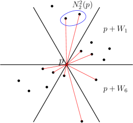
Figure 1: The wedges $p+W_{1},\ldots,p+W_{6}$ and the edges that are added to 2GNG$(P)$ ‘due’ to $p$.

Computing ${\rm 17GNG}(P)$ in general position.

Begin by assuming that $P$ is in general position. Actually, the only condition that we require is that no three points form an isosceles triangle. Computing ${\rm 17GNG}(P)$ in this case is relatively simple, since informally, the ranges that arise in computing ${\rm 17GNG}(P)$ are wedges with fixed orientations of their bounding rays. In contrast, the ranges that arise in computing ${\rm 17RNG}(P)$ are lenses formed by the intersection of two congruent disks, which are more expensive to process.

For each $p\in P$, we compute the set $N_{i}^{17}(p)$, for $i=1,\ldots,6$, which consists of the points that have at most 16 other points in $P\cap(p+W_{i})$ that are closer to $p$. When $P$ is in general position, these are the 17 closest points to $p$ in $P\cap(p+W_{i})$, see Figure 1. However, when this is not the case, $|N_{i}^{17}(p)|$ could be much larger, see Figure 2. (If $|P\cap(p+W_{i})|\leq 17$, then $N_{i}^{17}(p)=P\cap(p+W_{i})$.) We will later discuss the extension of the algorithm and analysis to degenerate situations.

We construct six similar data structures, where the $i$’th structure is used to compute the collection of sets $\{N_{i}^{17}(p)\mid p\in P\}$. The $i$’th structure is an augmented two-level ‘orthogonal’ range searching structure, where each level stores the points of (suitable canonical subsets of) $P$ in their order in the direction perpendicular to a bounding ray of $W_{i}$. For each node $v$ in the second level of the structure, we compute the 17th-order Voronoi diagram ${\rm Vor}_{17}(Q_{v})$ of $Q_{v}$, the canonical set of $v$, and store it at $v$ as a point-location structure. (Recall that ${\rm Vor}_{17}(Q_{v})$ partitions the plane into maximal regions, each with a fixed set of 17 closest sites.) The total size of the data structure is thus $O(n\log^{2}n)$, and it can be computed in total time $O(n\log^{3}n)$, where the Voronoi diagrams are computed by the algorithm of Chan and Tsakalidis [6], which takes $O(|Q_{v}|\log|Q_{v}|)$ deterministic time per diagram. (See also the earlier algorithm of Agarwal et al. [3], which is randomized and slightly less efficient.) In fact, since 17 is a constant, we can compute the diagram in a simpler incremental manner, starting with the standard diagram and adding one index at a time. This also takes $O(|Q_{v}|\log|Q_{v}|)$ time per diagram.

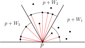
Figure 2: When $P$ is not in general position $|N_{i}^{2}(p)|$ could be larger than 2. Here, $|N_{1}^{2}(p)|=2$, $|N_{2}^{2}(p)|=5$, and $|N_{3}^{2}(p)|=3$.

Now, for each $p\in P$, we perform a query in the $i$’th structure to obtain the set $N_{i}^{17}(p)$. We initialize this set to be empty. We then identify the $O(\log^{2}n)$ second-level nodes, such that $P\cap(p+W_{i})$ is the disjoint union of their canonical sets. Next, we visit these nodes, one at a time, and at each node $v$ we perform a query with $p$ in ${\rm Vor}_{17}(Q_{v})$, and update $N_{i}^{17}(p)$ accordingly, in constant time. A query thus takes $O(\log^{3}n)$ time for each $p\in P$, for a total of $O(n\log^{3}n)$ time. (The latter bound follows since, in general position, each set $N_{i}^{17}(p)$ is of constant size (at most $17$)). The overall output of this procedure is the desired graph ${\rm 17GNG}(P)$.

Handling degeneracies.

When $P$ is not in general position, some modifications are required. As already observed, in this case $|N_{i}^{17}(p)|$ might be much larger than 17 (it could be even as large as $n-1$), although the total number of edges in ${\rm 17GNG}(P)$ remains $O(n)$ [7]. The problematic situation is when, for some $p\in P$ and some $1\leq i\leq 6$, and for some canonical set $Q$ of $P\cap(p+W_{i})$, there exists a large subset $Q^{\prime}$ of $Q$, all of whose points lie on a circle centered at $p$, with at most 16 points of $Q$ inside the circle. In that case all points of $Q^{\prime}$ form with $p$ potential edges of ${\rm 17GNG}(P)$, but to retain the aforementioned running time, we cannot afford to spend more than $O(\log n)$ time while processing $Q$ (when querying with $p$), unless they are indeed edges of ${\rm 17GNG}(P)$, in which case we may spend additional $O(|Q^{\prime}|)$ time. However, at this point we do not know whether they are edges of ${\rm 17GNG}(P)$, because other canonical sets might generate with $p$ shorter edges that exclude the potentially numerous longest edges involving $Q$ from the graph.

To address this issue, we modify the query with $p$ in the $i$’th structure as follows. As before, we first identify the $O(\log^{2}n)$ second-level nodes of the structure, such that $P\cap(p+W_{i})$ is the disjoint union of their canonical sets. The next stage consists of two rounds, where in each round we process each of these $O(\log^{2}n)$ nodes. The sole purpose of the first round is to find the distances $d_{1}<d_{2}<\cdots<d_{k}$, where $k\leq 17$, between $p$ and the $17$ closest points to $p$ among the points in $P\cap(p+W_{i})$. (We write $k\leq 17$, since the same distance may be attained by several points.) More precisely, if we were to sort the points in $P\cap(p+W_{i})$ by their distance from $p$, resolving ties arbitrarily, then $d_{1},\ldots,d_{k}$ would be the distinct distances corresponding to the first 17 points in the sequence. We now describe how to implement the first round in total $O(\log^{3}n)$ time, for each fixed $p$ and $i$, that is, in overall $O(n\log^{3}n)$ time.

We use the following notation. For a (two-dimensional open) cell $C$ of ${\rm Vor}_{17}(Q_{v})$, for some second-level node $v$, denote by $P(C)$ the set of the (uniquely defined) 17 closest points of $Q_{v}$ to any point in $C$. Moreover, for any point $p$ in the closure of $C$, put $d_{p}(C)=\max\{{\sf dist}(p,q)\mid q\in P(C)\}$.

For fixed $p$ and $i$, we maintain a sorted sequence $A=A_{p,i}$ of the 17 closest points to $p$ among the points of $P\cap(p+W_{i})$ that were encountered so far; initially $A$ is empty. (Ties are broken arbitrarily, and we limit the length of $A$ to 17 even when there are additional points, not in $A$, whose distance from $p$ is equal to that between $p$ and the last point in $A$.) At each second-level node $v$ of the structure, we locate $p$ in ${\rm Vor}_{17}(Q_{v})$, and proceed as follows. Let $C$ be a cell of the diagram such that $p$ lies in the closure of $C$ (the cell is not unique when $p$ lies on an edge or is a vertex of the diagram). Obtaining $C$ from the point location query is straightforward in all cases, and takes constant time. We update $A$ (or initialize it, if $v$ is the first visited node) by examining the points in $P(C)$. Specifically, we sort the set $P(C)$ by distance to $p$, and either copy the resulting sequence into $A$, when $v$ is the first processed node, or otherwise merge it with $A$, retaining only the first 17 elements.

Put $\Delta_{p,i}=\{{\sf dist}(p,q)\mid q\in A\}$, and note that $|\Delta_{p,i}|\leq 17$, where a strict inequality is possible. We have:

Lemma.

After processing all the $O(\log^{2}n)$ canonical sets that form $P\cap(p+W_{i})$, $\Delta_{p,i}$ is the set of distances between $p$ and the $17$ closest points to $p$ in $P\cap(p+W_{i})$.

Proof. We argue, by induction, that after processing some of the canonical sets, $\Delta_{p,i}$ is the set of distances between $p$ and the 17 closest points to $p$ in the union of these sets. The claim holds trivially initially, so assume that it holds just before processing some canonical set $Q$.

Let $C$ be the cell of ${\rm Vor}_{17}(Q)$ that is obtained from the point location query, so $p$ lies in the closure of $C$. The claim is easy to argue when $p$ lies in the interior of $C$, so the interesting case is when $p\in{\partial}C$. We observe that in this case, if $C^{\prime}$ is any other cell that contains $p$ (necessarily on its boundary) then $d_{p}(C^{\prime})=d_{p}(C)$ and

$$P(C^{\prime})\setminus\{q\in P(C^{\prime})\mid{\sf dist}(p,q)<d_{p}(C^{\prime})\}=P(C)\setminus\{q\in P(C)\mid{\sf dist}(p,q)<d_{p}(C)\}.$$

This follows directly from the definition of the diagram, since otherwise, either $P(C)$ or $P(C^{\prime})$ (or both) would not be the correct answer to the query with $p$. In other words, in this case it does not matter which of the cells that are adjacent to $p$ we use to update $A$. This property implies that the invariant is preserved after processing $Q$, and it therefore completes the induction step in this case too. $\Box$

In the second round, we iterate again over all points $p$ and indices $i$. For a fixed pair $p$ and $i$, we retrieve the $O(\log^{2}n)$ canonical sets that form $P\cap(p+W_{i})$. For each of these sets $Q$, we locate $p$ in ${\rm Vor}_{17}(Q)$ and compute $d_{p}(C)$ in constant time, for some (single) cell $C$ of the diagram whose closure contains $p$ (recall that this value is independent of $C$). We then compute the set $\Delta_{p,i}(C)$ of distances between $p$ and the points of $P(C)$ that belong to $\Delta_{p,i}$, i.e., $\Delta_{p,i}(C)=\{d\in\Delta_{p,i}\mid d={\sf dist}(p.q)\text{ for some }q\in P(C)\}$. Two cases can arise:

(i) $d_{p}(C)\notin\Delta_{p,i}(C)$. In this case the subset $P_{p}(C)$ of $P(C)$ of the points whose distances to $p$ are in $\Delta_{p,i}(C)$ is independent of the cell $C$ (as long as $C$ contains $p$ in its closure). We then simply find $P_{p}(C)$ and add to ${\rm 17GNG}(P)$ all the (at most 16) edges $(p,q)$ for $q\in P_{p}(C)$.

(ii) $d_{p}(C)\in\Delta_{p,i}(C)$. In this case we iterate over all the cells $C$ incident to $p$, and add all the edges $(p,q)$, for $q\in\bigcup_{C}P(C)$. This does not affect the asymptotic bound on the running time: if there are $k$ such cells, we process $O(k)$ points but add $\Theta(k)$ edges to ${\rm 17GNG}(P)$, as is easily checked. (If $p$ is adjacent to $k$ cells then there are $k$ points in $Q$ at distance $d_{p}(C)$ from $p$, and all of them form with $p$ edges of ${\rm 17GNG}(P)$.)

By applying this procedure to each $p$ and $i$ and to each corresponding canonical set $Q$, we obtain the desired graph ${\rm 17GNG}(P)$.

Wrapping it up.

We have shown that one can compute ${\rm 17GNG}(P)$ in $O(n\log^{3}n)$ time. Having computed ${\rm 17GNG}(P)$, we continue as before, running a binary search over its $O(n)$ edge lengths, using the algorithm of Bonnet et al. [5] to guide the search. In summary, we obtain:

Theorem.

A bottleneck matching of a set of $n=2\ell$ points in the plane can be computed in $O(n^{\omega/2}\log n)$ deterministic time.

Abu-Affash et al. [1] presented an algorithm that, given a perfect matching $M$ of $P$, returns in $O(n\log n)$ time a non-crossing perfect matching $N$ of $P$, such that $\lambda(N)\leq 2\sqrt{10}\lambda(M)$. We thus obtain:

Corollary.

A non-crossing perfect matching $N$ of a set of $n=2\ell$ points in the plane with $\lambda(N)\leq 2\sqrt{10}\lambda^{*}$ can be computed in $O(n^{\omega/2}\log n)$ deterministic time, where $\lambda^{*}$ is the length of a longest edge in a bottleneck matching of $P$.

References

- [1] A. K. Abu-Affash, P. Carmi, M. J. Katz and Y. Trabelsi, Bottleneck non-crossing matching in the plane, Comput. Geom. 47 (2014), 447–457.
- [2] P. K. Agarwal, B. Aronov, M. Sharir and S. Suri, Selecting distances in the plane, Algorithmica 9 (1993), 495–514.
- [3] P. K. Agarwal, M. de Berg, J. Matoušek and O. Schwarzkopf, Constructing levels in arrangements and higher-order Voronoi diagrams, SIAM J. Comput. 27 (1998), 654–667.
- [4] J. Alman and V. Vassilevska Williams, A refined laser method and faster matrix multiplication, Proc. ACM-SIAM Sympos. on Discrete Algorithms (SODA), 2021, 522–539.
- [5] É. Bonnet, S. Cabello and W. Mulzer, Maximum matchings in geometric intersection graphs, Proc. 37th Internat. Sympos. on Theoretical Aspects of Computer Science (STACS), 2020, 31:1–31:17. See also, arXiv:1910.02123.
- [6] T. M. Chan and K. Tsakalidis, Optimal deterministic algorithms for 2-d and 3-d shallow cuttings, Discrete Comput. Geom. 56 (2016), 866–881.
- [7] M. S. Chang, C. Y. Tang and R. C. T. Lee, Solving the Euclidean bottleneck matching problem by -relative neighborhood graphs, Algorithmica 8 (1992), 177–194.
- [8] B. N. Clark, C. J. Colbourn and D. S. Johnson, Unit disk graphs, Discrete Math. 86 (1990), 165–177.
- [9] H. N. Gabow and R. E. Tarjan, Algorithms for two bottleneck optimization problems, J. Algorithms 9 (1988), 411–417.
- [10] F. Le Gall, Powers of tensors and fast matrix multiplication, Proc. 39th Internat. Sympos. on Symbolic and Algebraic Computation (ISSAC), 2014, 296–303.
- [11] T.-H. Su and R.-C. Chang, Computing the k-relative neighborhood graphs in Euclidean plane, Pattern Recognition 24 (1991), 231–239.