Improved Sensitivity for Space Domain Awareness Observations with the Murchison Widefield Array

Abstract

Our previously reported survey of the Low Earth Orbit (LEO) environment using the Murchison Widefield Array (MWA) detected over 70 unique Resident Space Objects (RSOs) over multiple passes, from 20 hours of observations in passive radar mode. In this paper, we extend this work by demonstrating two methods that improve the detection sensitivity of the system. The first method, called shift-stacking, increases the statistical significance of faint RSO signals through the spatially coherent integration of the reflected signal along the RSO’s trajectory across the sky. This method was tested on the observations used during our previous blind survey, and we obtained a $75\%$ increase in the total number of detections. The second method re-focuses the MWA to the near-field RSO’s position (post-observation), by applying a complex phase correction to each visibility to account for the curved wave-front. The method was tested successfully on an MWA extended array observation of an ISS pass. However, the method is currently limited by signal de-coherence on the long-baselines (due to the hardware constraints of the current correlator). We discuss the sensitivity improvement for RSO detections we expect from the MWA Phase 3 correlator upgrade. We conclude the paper by briefly commenting on future dedicated Space Domain Awareness (SDA) systems that will incorporate MWA technologies.

1 INTRODUCTION

The onset of the Kessler Syndrome [10], a cascading collision event scenario in the near-Earth environment, can be delayed or prevented by preforming space surveillance. The current rapid increase in the number of Resident Space Objects (RSOs) in the Low Earth Orbit (LEO) demands the development of multiple Space Domain Awareness (SDA) sensors, that together contribute towards the global SDA effort. Most of the current SDA activities are undertaken by the Space Surveillance Network (SSN) [14] based in the US and its European equivalent operated by the European Space Agency (ESA) [3]. The majority of the existing SDA facilities consist of either optical sensors that perform space surveillance during twilight or active coherent radars that perform searches for RSO reflections (we direct the reader to [15] for a detailed summary of current SDA radar systems and how the non-coherent MWA radar system employed in this work is novel compared to existing solutions). Both of these types of systems often have a small Field of View (FOV), thus limiting their capability to perform simultaneous detections.

In the recent past, there has been a growing interest in decentralising SDA information across different countries in order to prevent “bias of information” [11]. We aim to address these issues by using an already existing wide FOV radio telescope, the Murchison Widefield Array (MWA) [25] [30], as a passive radar to perform space surveillance by searching for RSO reflections of terrestrial FM transmissions. The MWA is an international effort by different countries and its data are publicly available. In this paper, we build upon our previous SDA work with the MWA, and demonstrate two different techniques that provide more sensitive RSO signal detections.

In our previous survey of the LEO environment using the MWA [20], we demonstrated blind detection techniques for detecting RSOs, meteors, and aircraft using MWA observations. Whilst blind searches are a good method for detecting lost/new RSOs, in this paper we perform more sensitive detections of faint RSO signals by using prior knowledge of their trajectory to integrate the signal across the sky.

The first method that we explore in this work is called “shift-stacking”. The shift-stacked RSO search method uses phase-tracked difference images to perform detections by integrating the signal along the predicted trajectory of the pass. Although shift-stacking has been previously described in the literature to search for new Kuiper belt objects, trans-Neptunian objects [2] such as “Planet Nine” [22], and solar-system satellites [4] by trial and error iterations performed in a multi-dimensional parameter space, we adapt this method to perform searches for weak RSO signals in MWA data. A similar method has been also previously explored by [23] for optical SDA sensors.

The second method that is demonstrated in this paper aims to improve the detection of RSO signals by re-focusing the interferometer (the MWA) to the predicted near-field RSO position. Standard interferometer theory assumes the observed source to be in the far-field of the instrument, thus deriving a 2D Fourier relationship between the re-constructed sky image and the measured visibilities. However, due to the near-field nature of the LEO RSOs, the longer baselines of the MWA see a curved wave-front rather than a planar wave-front. Hence, when imaged (without accounting for the curvature), the satellite signal appears de-focused, resulting in reduced signal to noise. In this work, we demonstrate a near-field RSO search performed using the MWA and also address its current limitations due to hardware constraints.

This paper is structured as follows. In Section 1.1 we briefly describe the MWA and the SDA techniques. In Section 2 we describe the observations used and the data processing methods employed. The results of the analysis performed are provided in Section 3, followed by a brief discussion. We draw our conclusions in Section 4.

1.1 BACKGROUND

Most of the current SDA sensors are concentrated in the northern hemisphere. The development of SDA capability using the limited land in the Southern Hemisphere is therefore of international importance. Hence, since the MWA has been shown in the past to be capable of performing SDA observations, we continue our effort to develop further the sensitivity of the MWA SDA system. The development of more sensitive detection methods was also motivated by our participation in Space Fest 2020, an Australian Airforce sponsored civilian event, when different SDA groups from around Australia came together to demonstrate their SDA capabilities. Based in part on the demonstrations performed during Space Fest, future dedicated SDA facilities may be constructed.

The MWA [25] is a low-frequency radio interferometer located at the radio quiet Murchison Radio-astronomy Observatory (MRO), Western Australia. The MWA is capable of observing the southern radio sky between $70-300$  MHz using $128$ tiles, with an instantaneous bandwidth of $30.72$ MHz. The MWA underwent an upgrade to Phase $2$ during 2016 [30], using the same hardware as the Phase $1$ array, but with an additional $128$ tiles deployed. The MWA Phase 2 array is periodically reconfigured between the extended configuration and the compact configuration, each of which contains $128$ tiles [30]. The extended configuration has baseline lengths up to $5.3$ km and has a higher angular resolution, while most of the compact configuration baselines are under $200$ m to provide increased sensitivity to extended emission.

The MWA previously demonstrated SDA by performing coherent SDA radar detections [19][5][6] using the MWA’s Voltage Capture System [28], as well as non-coherent SDA radar detections [26][31][21][20] using the MWA’s standard operation mode (as an aperture synthesis array). By using the line of sight FM transmission as the reference signal, the coherent radar method uses matched filtering to identify satellite reflections. The non-coherent radar method performs source finding on difference images to search for satellite signals. In this paper, we continue to develop the non-coherent method, and the reader is referred to the aforementioned papers for more information about the MWA’s coherent SDA system.

The non-coherent MWA SDA system performs RSO detections by searching for time-varying signals in fine-channel ($40$ kHz wide) difference images. [31] demonstrated difference imaging to be an effective technique to search for RSOs in MWA observations, as it subtracts the static background sources along with its side-lobe confusion noise and is only limited by the thermal noise of the instrument. RSO signals in difference images appear as a streak with a positive head and a negative tail, as shown in Figure 1 and Figure 8.

2 DATA AND METHODS

2.1 Shift-Stacking

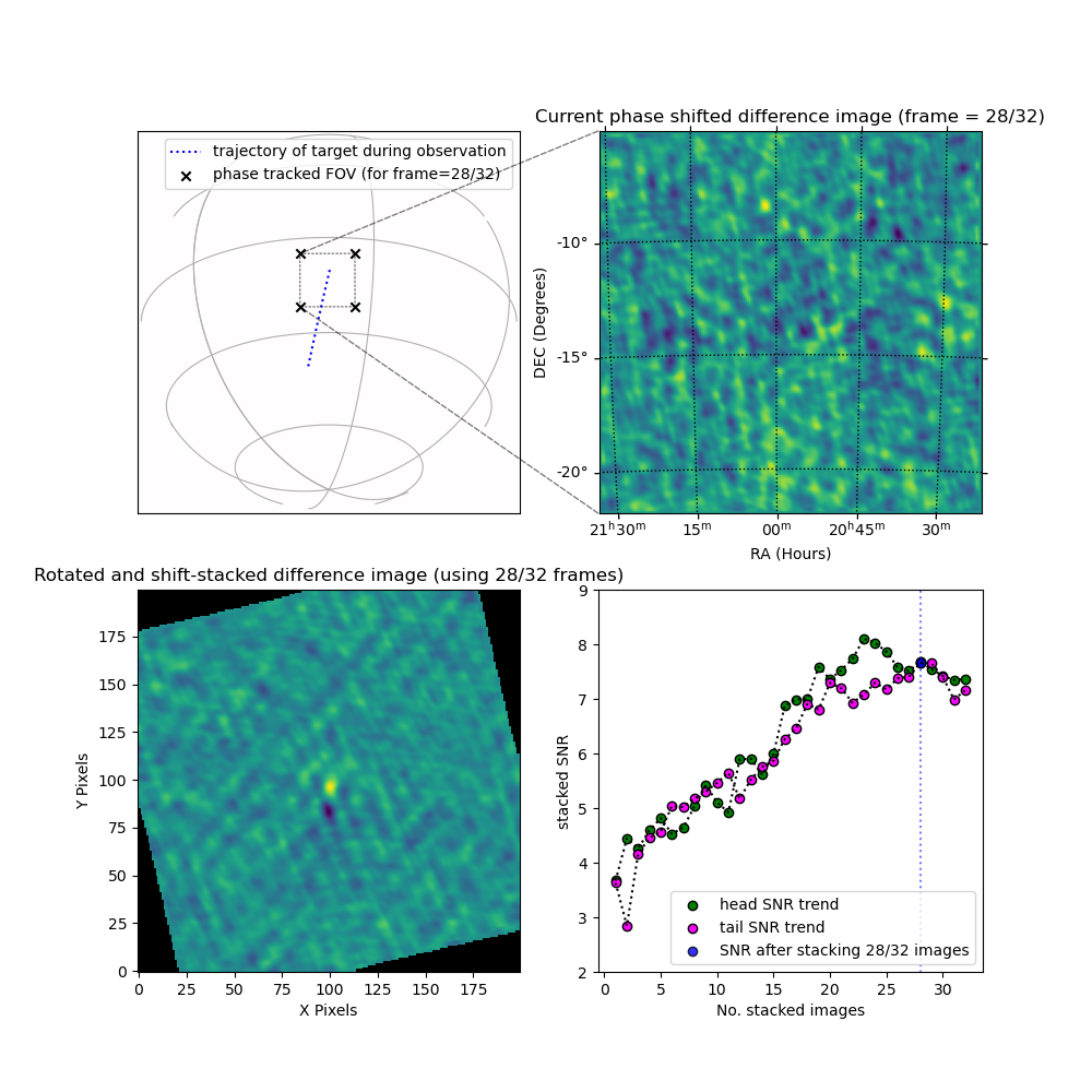
Figure 1: Demonstration of detection performed using the shift-stacking method. The top left-panel is the entire horizon visible to the MWA during the observation. The predicted trajectory of the satellite (blue dotted line) and the phase tracked FOV of the satellite for frame $N=28$ (black crosses) are shown. The insert panel (top-right) shows the phase-tracked fine channel difference image for the considered time-step/frame. The bottom-left panel is the rotated shift-stacked fine channel difference image of the RSO signal after stacking N frames (in this case $N=28$). An animation of this figure is available at https://www.youtube.com/watch?v=_dbEW61RnFk. The bottom-right panel shows the SNR of the RSO signal increasing with the number of stacked frames.

We test the shift-stacking method using the $20$ hours of Phase 2 compact configuration observations used in our previous blind survey [20]. For the MWA, the GPS time of the observation is used as the observation ID, and observations can be obtained from the All-Sky Virtual Observatory (ASVO). Re-using the observations in this work allows us to compare the performance of the previously demonstrated blind detection method and the shift-stacking detection method developed here. The visibilities are calibrated (using the calibrate tool developed in [18]) and converted to CASA measurement set format [13] as explained in [20], and the fine frequency channel images are created using WSClean [16][17].

The shift-stacking method seeks to detect RSOs by performing a spatially coherent averaging of the signals along the predicted trajectory. An example of shift-stacking for the object PICOSAT-9 (NORAD ID $26930$) during the observation ID $1157400472$ is demonstrated in Figure 1. The top-left panel shows the predicted trajectory of the RSO above the visible horizon and the phase-tracked field-of-view (FOV) of an individual shift-stack frame. Due to the large FOV of the MWA (approx. $1300$ degree²), the curvature of the RSO pass is often resolved (i.e, the apparent direction of the RSO motion changes during the pass) and stacking without any orientation correction would result in signal smearing. Hence we rotate the individual frames (using scipy.ndimage.rotate) to align the signal in the vertical direction (arbitrarily chosen) prior to stacking. The bottom-left panel of Figure 1 shows the rotated shift-stacked difference image (after performing an inverse-noise weighted stacking of $N$ frames) for one fine frequency channel.

All LEO RSOs that were predicted to pass through the MWA’s primary beam during the observations were identified. For every identified object, we search for the satellite signal at every $40$ kHz fine frequency channel using the shift-stacking pipeline (resulting in a stacked image cube). Prior to stacking, the phase centre of each of the individual frames is centred (using the chgcentre tool developed by Andre Offringa) at the predicted location of the object during the epoch, thus enabling spatially coherent stacking of the faint RSO signal along the RSO’s trajectory.

All $6\sigma$ detections that appeared as the expected streak signal were identified from the shift-stacked image cube (the third dimension being frequency). We vet the detections to obtain a preliminary list of candidate detections using the criterion that the detection must appear as a spatially coherent $6\sigma$ streak in more than one fine frequency channel. This helps get rid of aliased side-lobes of other bright events that may spatially coincide with the object of interest and this is also the selection criterion used during our previous blind survey. The list of $164$ detected candidates are further investigated in Section 3.

2.2 Near-Field Re-Focusing

The RSO reflected wavefronts appear curved when observed using the long MWA baselines, resulting in de-focused (reduced SNR) signals. This apparent deviation ($\Delta w$) from a planar wave-front as seen by a “long” baseline is shown in Figure 2. Since the Phase $2$ compact configuration array has the majority of its baselines shorter than $200$ m, LEO RSOs would appear in the far-field of the instrument and therefore no re-focusing is required. We therefore focus our efforts on the Phase $2$ extended array (observation ID $1290483224$ that had the ISS pass through the primary beam) which has predominantly long baselines that sees the RSO in the near-field. The ISS observation was calibrated using amplitude and phase solutions obtained for the observation ID $1290513616$ (infield GLEAM sources [8] were used as the model for the sky based calibration performed, followed by the application of self-calibration). The two observations were approximately $8$ hours apart and MWA calibration solutions are generally valid within a day.

Prior knowledge of the RSO’s and MWA tile’s Geocentric Cartesian coordinates (e.g, $X_{rso}$, $Y_{rso}$, $Z_{rso}$ and $X_{tile1}$, $Y_{tile1}$, $Z_{tile1}$) are used to calculate the actual deviation/delay from a planar wave-front ($\Delta w$ in Figure 2) as seen by each baseline (calculated independently for every time-step within the observation). The calculated delay $\Delta w$ is applied as a phase offset to re-focus the array to the desired near-field location. For a baseline between $tile_{1}$ and $tile_{2}$, $\Delta w_{1-2}$ is calculated using Equation 1

$$\begin{array}[]{l}R_{1}^{2}=(X_{rso}-X_{tile1})^{2}+(Y_{rso}-Y_{tile1})^{2}\\ \qquad\qquad\qquad\quad+(Z_{rso}-Z_{tile1})^{2}\\ R_{2}^{2}=(X_{rso}-X_{tile2})^{2}+(Y_{rso}-Y_{tile2})^{2}\\ \qquad\qquad\qquad\quad+(Z_{rso}-Z_{tile2})^{2}\\ \Delta w_{1-2}=(R_{1}-R_{2})-w_{1-2}\par\end{array}$$ (1)

where $R_{1}$($R_{2}$) is the distance in metres between the RSO and $tile_{1}$($tile_{2}$). $\Delta w_{1-2}$ is the w-term associated with a planar wave-front as seen by the baseline. The calculated delay is applied to the measured visibility as a complex phase offset using Equation 2 (adapted from [12]),

$$\Delta phase_{1-2}=\exp^{i2\pi\frac{\Delta w_{1-2}}{\lambda}},$$ (2)

where $\lambda$ is the wavelength of the fine frequency channel. The correction is applied to the visibilities set prior to imaging using our python tool LEOVision. Results are discussed in Section 3.

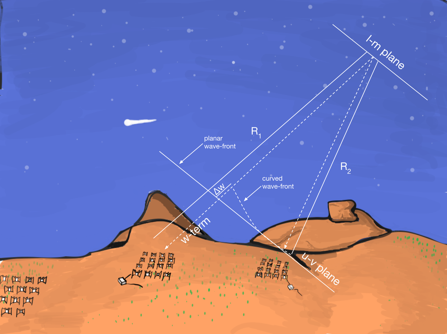
Figure 2: The near-field curvature as seen by a baseline-pair. $\Delta w$ is the delay due to the curved wave-front and $R_{i}$ is the distance between the RSO and $tile_{i}$.

3 RESULTS AND DISCUSSION

3.1 Shift-Stacking Candidates

Through manual inspection of the $164$ candidates obtained from the shift-stack search performed in Section 2.1, we identify two different types of detections, namely, flaring events (64) and steady reflection events (100). Flaring events often have a single frame with a very high SNR signal, where stacking reduces the SNR of the detection (due to a lack of spatially coherent signals in other frames). An example of a flaring event is shown in Figure 3. On the contrary, the SNR of steady reflection events only increases with stacking and an example is shown in the bottom panels of Figure 1.

Figure 3: An example of a flaring event detected using the shift-stack pipeline. Figure shows the SNR of the RSO signal reducing with the number of stacked frames.

The two different populations of candidates are further analysed based on their offset from the phase centre (predicted location of the object using previously estimated orbital parameters) of the shift-stacked image, and the frequency channel they are detected in. While the frequency channel investigation helps determine if the event is due to an FM reflection from RSOs, or bad difference imaging (imperfect background source subtraction due to time varying sky signal or instrument response), the apparent offset helps determine if the detected signals are likely to be from the RSO of interest.

Figure 4 shows the centroid offset (projected into in-track and cross-track directions) for all the flaring and steady reflection events, and we see very different behaviour between the two populations. The majority of the steady reflection events appear within a degree of the phase centre (expected location of the object), while the flaring events have an almost uniform distribution of offsets before tapering off near the edge of the shift-stacked FOV. This tapering is due to image rotation resulting in many blank pixels near the edge as seen in the bottom-left panel of Figure 1.

As most of the steady reflection events are closer to the predicted locations than the flaring events, they are more likely to be from the RSO of interest, and hence we classify them as our final list of candidate detections. We detect almost all the RSOs detected during our blind survey [20], except a few RSOs where a few noisy frames reduced the stacked SNR of the RSO signal below the detection threshold used in Section 2.1). We also detect many more new RSOs not previously detected. Using shift-stacking, we improve the total number of RSO detection candidates from our $20$ hours of observation by $75\%$. The list of new detections (excluding the events already detected during the blind survey in [20]) is given in Table 1. Note that for the MWA, primary beam correction is applied in the image domain, and creating the corresponding phase tracked primary beam models for every time-step is a very computationally intensive task, as the individual shift-stack frames were not primary beam corrected. Hence, Table 1 provides only the apparent peak flux density of the detections and can be treated as a lower limit on the actual flux density of the detection. The in-track and cross-track offsets measured for every steady reflection event (shown in Figure 4) can also be used for performing orbital element updates for the RSOs.

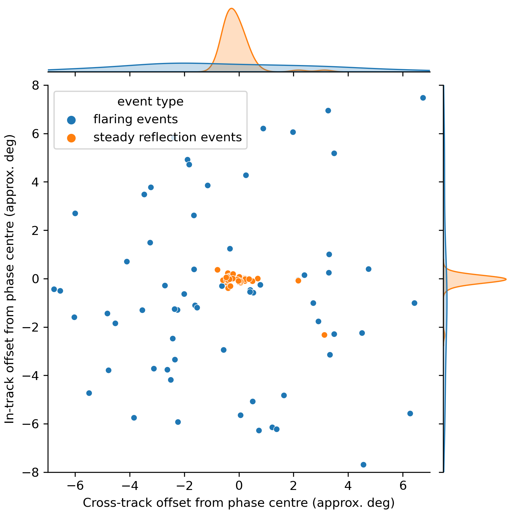
Figure 4: The apparent centroid offset distribution for steady reflection and flaring events. Most of the steady reflection events are within a degree of the predicted location, while the flaring events have almost a uniform distribution within the FOV and tapers off towards the edge due to rotating the frames prior to stacking.

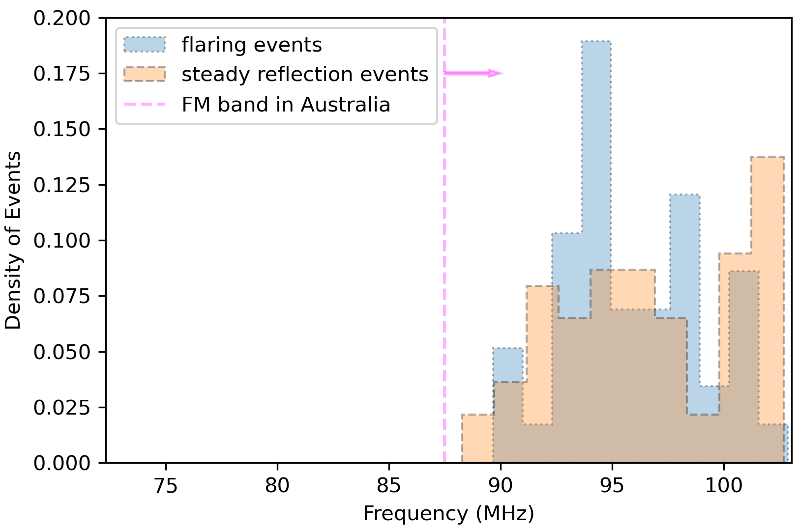
Figure 5: The density distribution of channels in which the flaring and steady reflection events were detected. The two brightest channels at which the event was detected spatially coherent (channels identified during the candidate vetting process in Section 2.1) was used to create the plot. We see that all the steady reflection events are confined within the FM band (as expected), and all of the flaring events were also detected within the FM band, implying that many of the flaring events could be FM reflections from other real events such as meteors trails.

The frequency of the observations used in the shift-stack analysis span $72.335-103.015$ MHz, while the FM band only overlaps with the second half of the observation band (i.e, above $88$ MHz). Figure 5 shows the frequency distribution of all the detected steady reflection and flaring events. From Figure 5 we see that all the steady reflection events are confined within the FM band (as expected from FM reflecting RSO) and all of the flaring events are also confined within the FM band. Hence, it is very likely that the flaring events, though not the RSOs searched for, are real reflection events (and not due to noise). Many ($8.5$ hours) of the observations used coincided with the Geminids meteor shower and it is likely that many of the flaring events are associated with FM reflections from ionised meteor trails. The occurrence of these FM reflecting flaring events are consistent with a recent study of the RFI environment at the MRO by [27].

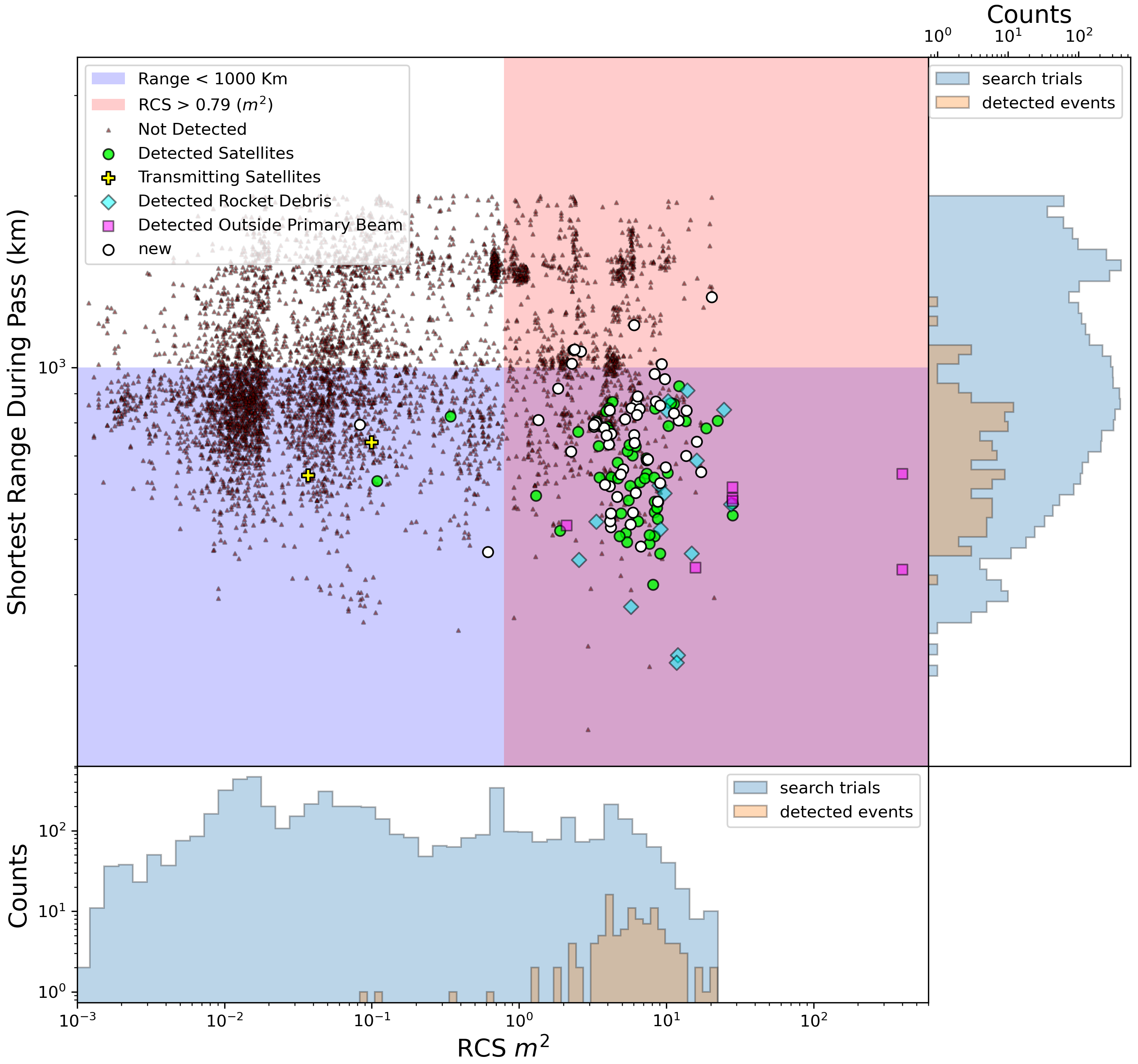
Figure 6: New candidate detections (steady reflections) in range vs RCS parameter space using white circle markers. The background image is the detection summary of the blind survey performed in [20]. Note that the objects detected outside the primary beam were not considered in the histograms plotted along the right and lower axes.

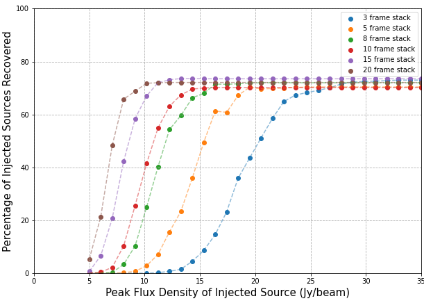
Figure 7: Figure shows the percentage of injected synthetic sources recovered by our detection pipeline for different number of images/time-steps stacked. Note that the vertical scatter on the maximum recovery parentage for different number of frames stacked is within the error of the simulation. They often converged very close to the theoretical limit upon using large number of search trials, but were not performed here due to the process being computationally expensive.

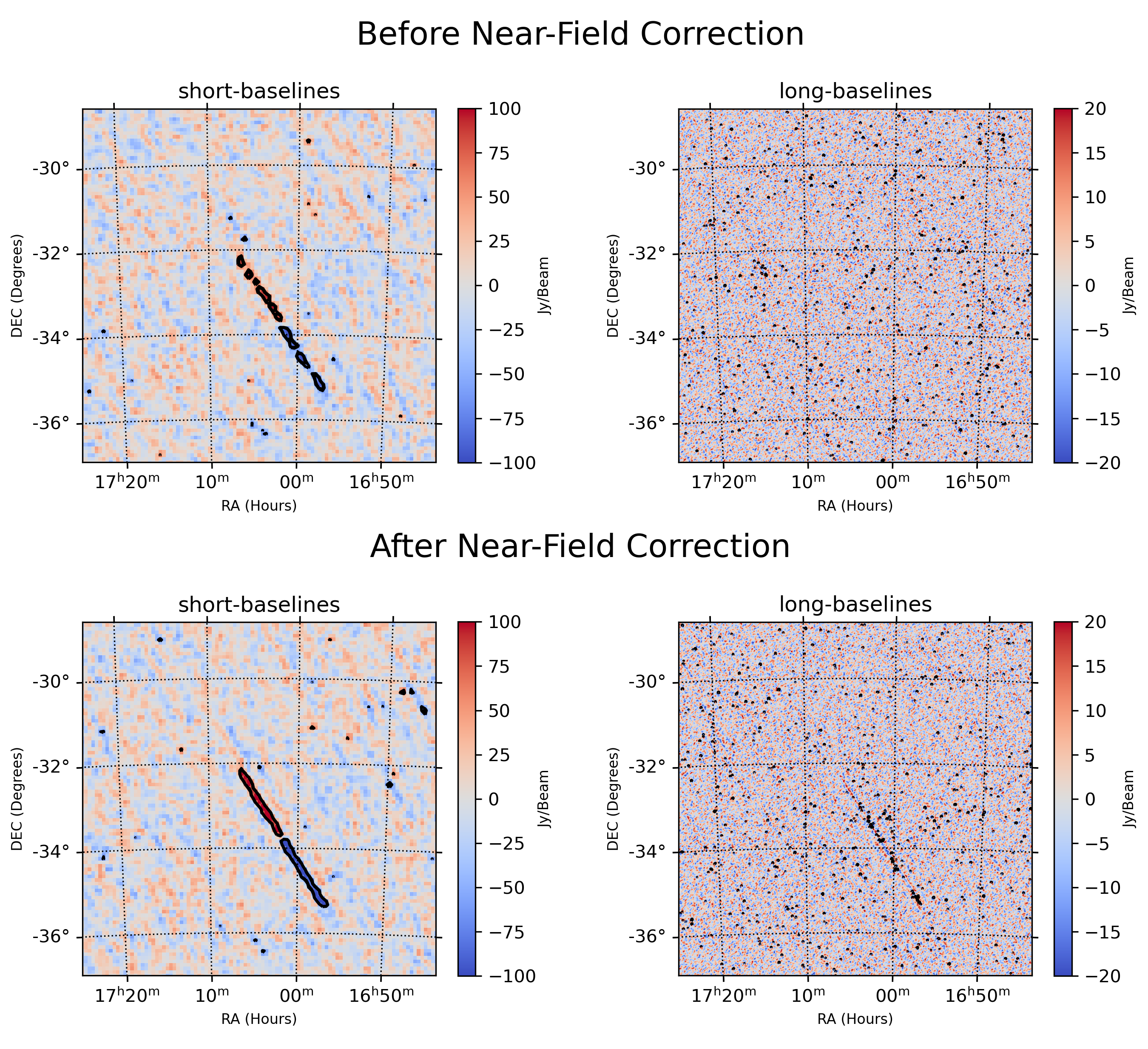
Figure 8: Demonstration of the near-field imaging capability with the MWA. The top two panels are the short-baseline and long-baseline difference image of a single fine channel at a given time-step, prior to applying the required phase correction. The long/short baseline cut-off used is $826$ m, as determined by the near-field equation. In all the four panels, we use black contours to help identity bright pixels in the image (pixels whose absolute value is greater than 60 in the short baseline images and pixels whose absolute value is greater than 25 in the long baseline images). The fits files used to make the above figure can be obtained from https://zenodo.org/record/5493585#.YThmjO0zZhE.

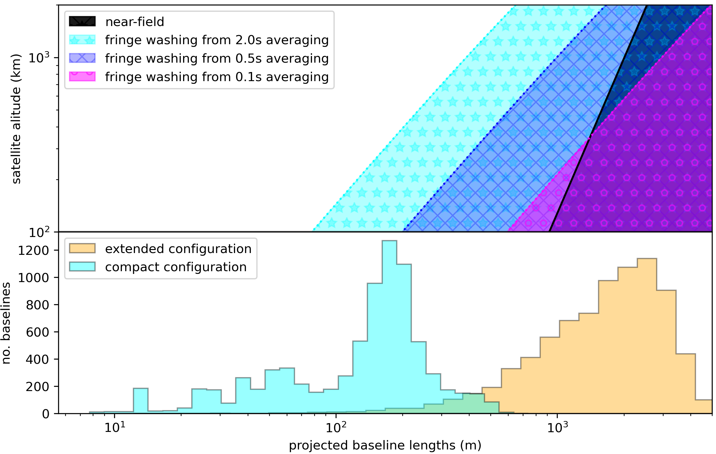
Figure 9: Top panel shows the baselines affected by the near-field effect and fringe-washing (phase change of $\pi$) as a function of satellite altitude (angular speed). The bottom panel of the figure shows the baseline length distribution for the phase 2 compact and extended configuration.

The final list of new detection candidates (from Table 1) from the shift-stack targeted search is shown in the Radar Cross-Section (RCS) vs range parameter space in Figure 6. The background image is the blind survey detection summary figure from [20], and the new detections are annotated using white circle markers. The histograms along the right and lower axes of Figure 6 show the distribution of all the search trials performed using shift-stack in this paper (blue) along with the total number of detections (blind survey and shift-stack in orange) obtained inside the primary beam during the observations used. The blue histogram shows the parameter space probed during the search, and the orange is what was detected (completeness of the technique) using the non-coherent methods developed in [20] and this paper. We also show the region with RCS $>0.79$ m² and range $<1000$ km as the parameter space [26] predicts the MWA to be sensitive towards. The majority of the detections do fall within the predicted region. Within the predicted parameter space (bottom-right quadrant of Figure 6), we detect $20\%$ of the objects that passed through the primary beam. The remaining objects were likely not detected due to non-favourable transmitter-RSO-MWA reflection geometries during the pass. Also, the RCS values plotted in Figure 6 are very likely to be much smaller in the observed FM wavelengths(hence we use them as a size order of magnitude guide only).

3.1.1 Shift-Stacking Completeness

We quantify the completeness of our shift-stacking search by performing an injection and recovery test. We inject 2D Gaussian sources of varying peak flux density into real MWA images and calculate our recovery rates. Since in Section 2.1 we only classify events with spatially coherent signal in more than one fine channel as a detection (to remove false positives from aliased side-lobes of other bright events), we inject the synthetic source in two fine-channels and attempt to recover them. Doing so helps us also estimate the number of false-negatives in our method due to one of the injected fine frequency channels being noisier than the other (resulting in the source being recovered in only one of them). Performing the injection and recovery test using real MWA images also helps determine the impact of the instrument’s thermal noise on the detection rate, and accurately captures the impact of increased confusion noise from other FM band events (such as meteor scatter, atmospheric FM ducting, and other RSOs within the FOV). Different RSOs were visible for different duration, (resulting in different number of frames stacked) within the MWA’s primary beam, and hence we also test our recovery rates for different number of frames stacked.

For a given peak flux density ($S_{peak}$) and number of frames stacked ($N$), we perform $1000$ search trails (arbitrarily chosen large number) to estimate our recovery rates, and the steps involved in the injection recovery test is given below.

• Step1: randomly choose two different fine channels within the FM band;

• Step2: retrieve $N$ difference images in the chosen fine channels;

• Step3: inject synthetic source in each frame of peak flux density $S_{peak}$; and

• Step4: stack frames and attempt recovering the synthetic source. Note the event is classified as a detection only if its is detected over $6\sigma$ in both the fine channels.

The percentages of sources recovered is shown in Figure 7, and we see that we can recovery only approximately about $72$ percent of the sources. This is in agreement with our expectation as about $25$ percent of the fine channels in our observations were flagged due to non-linear band-pass characteristics of the MWA’s poly-phase filter bank.

3.2 Near-Field Analysis

The ISS passed through the primary beam of an extended array observation, and hence is used as the object of interest in this section. The motivation for using the ISS is two-fold. First, it is a large-sized object which gives consistent reflections at multiple frequencies and secondly, it is a particularly low orbit RSO and thus is in the near-field more often than other large objects. For one of the time-steps that the ISS was detected, the MWA’s baselines were divided into short and long baselines (using $826$ m as the cut-off for the baseline separation, as determined by the near-field approximation $d<2D^{2}/\lambda$, where $\lambda$ is the wavelength, $D$ is the baseline length, and $d$ is the far-field distance), and the corresponding fine-channel difference images are shown in the top panels of Figure 8. We see that the streak signal is detected above $6\sigma$ in the short baseline image while it is not detected using the long baselines.

The near-field visibility phase correction for the appropriate time-step is applied using the LEOVision python tool. The phase-corrected difference images for the short and the long baselines are shown in the bottom panels of Figure 8. While the SNR of the short baseline image has increased, the previously undetected streak signal in the long baseline image now begins to appear. This demonstrates the MWA’s capability to focus on the desired near-field RSO position to perform more sensitive SDA detections.

Although the signal was recovered in the long-baseline difference image after applying the phase correction, the SNR in the long-baseline difference image is much lower than the short-baseline SNR, contrary to our expectation. When the baseline cut-off was applied, $1365$ baselines were classified as short baselines and the remaining $6636$ baselines were classified as long baselines (note only $8001$ baselines were available after flagging). Because the long-baseline image has more collecting area (number of baselines), we expect it to detect the RSO signal at a higher SNR than the short baseline image, contrary to what we see in Figure 8. We attribute this effect to the fringe-washing of the RSO signal on the long baselines. The phase of the measured complex visibility contains information about the source position with respect to the phase-centre. The visibility averaging duration (limited to $0.5$ s with the current MWA hardware) of the correlator is often optimised to minimise fringe-washing of celestial sources due to sidereal rotation ($0.25^{\circ}/minute$ on the equator). However, the phase of the fast moving LEO objects (e.g, ISS moves at approx. $60^{\circ}/minute$ near the zenith) considered in this work changes rapidly within the time averaging duration, thus resulting in a loss of coherence (fringe-washing) when using the long baselines. The baseline lengths affected by fringe-washing when observing an object at an altitude $alt$ can be obtained from Equation 3 (the equation is derived in Appendix A),

$$\begin{array}[]{l}\Delta\text{phase}\approx 2\pi\frac{\displaystyle b}{\displaystyle\lambda\times alt}\sqrt{\frac{\displaystyle GM_{earth}}{\displaystyle R_{earth}+alt}}\Delta t\par\end{array}$$ (3)

where $\Delta\text{phase}$ is the change in visibility phase, $\Delta t$ is the visibility averaging duration in $s$, $b$ is the length (in $m$) of the baseline component parallel to the satellite motion, $\lambda$ is the wavelength in $m$, G ($m^{3}kg^{-1}s^{-2}$) is the gravitational constant, $M_{earth}$ ($kg$) is the mass of Earth, and $R_{earth}$ ($m$) is the radius of Earth. Using Equation 3, we show the baseline lengths (parallel to the motion of the satellite, and the parallel component of baselines of other orientations) affected by the fringe-washing effect (visibility phase change of $\pi$ radians) in the top panel of Figure 9 (for $2.0$ s, $0.5$ s, and $0.1$ s visibility averaging). Note that the figure also shows the baseline lengths affected by the near-field effect (independent of the visibility averaging duration).

The bottom panel of Figure 9 also shows the baseline distribution of the MWA Phase 2 extended array and the compact array. As we go from short baselines towards the longer baselines, from Figure 9, we see that the fringe-washing comes into effect much before the near-field de-focusing effect (plotted using equation $d<2D^{2}/\lambda$) for the $2$ s time-averaging used. Hence, in Figure 8 we cannot recover the RSO signal with the longer baseline difference image due to fringe-washing. However, with the Phase 3 MWA, we will be able to sample visibilities with $0.1$ s time-averaging and more sensitive SDA observations with longer baselines should be possible. The minimum number of baselines not fringe-washed as a function of altitude is shown in Figure 10. We see that the sensitivity of the extended array with the new Phase 3 correlator ($0.1$ s averaging) is more sensitive (as more baselines are not fringe-washed) than the current hex configuration blind survey performed in [20] (compact configuration with $2$ s averaging).

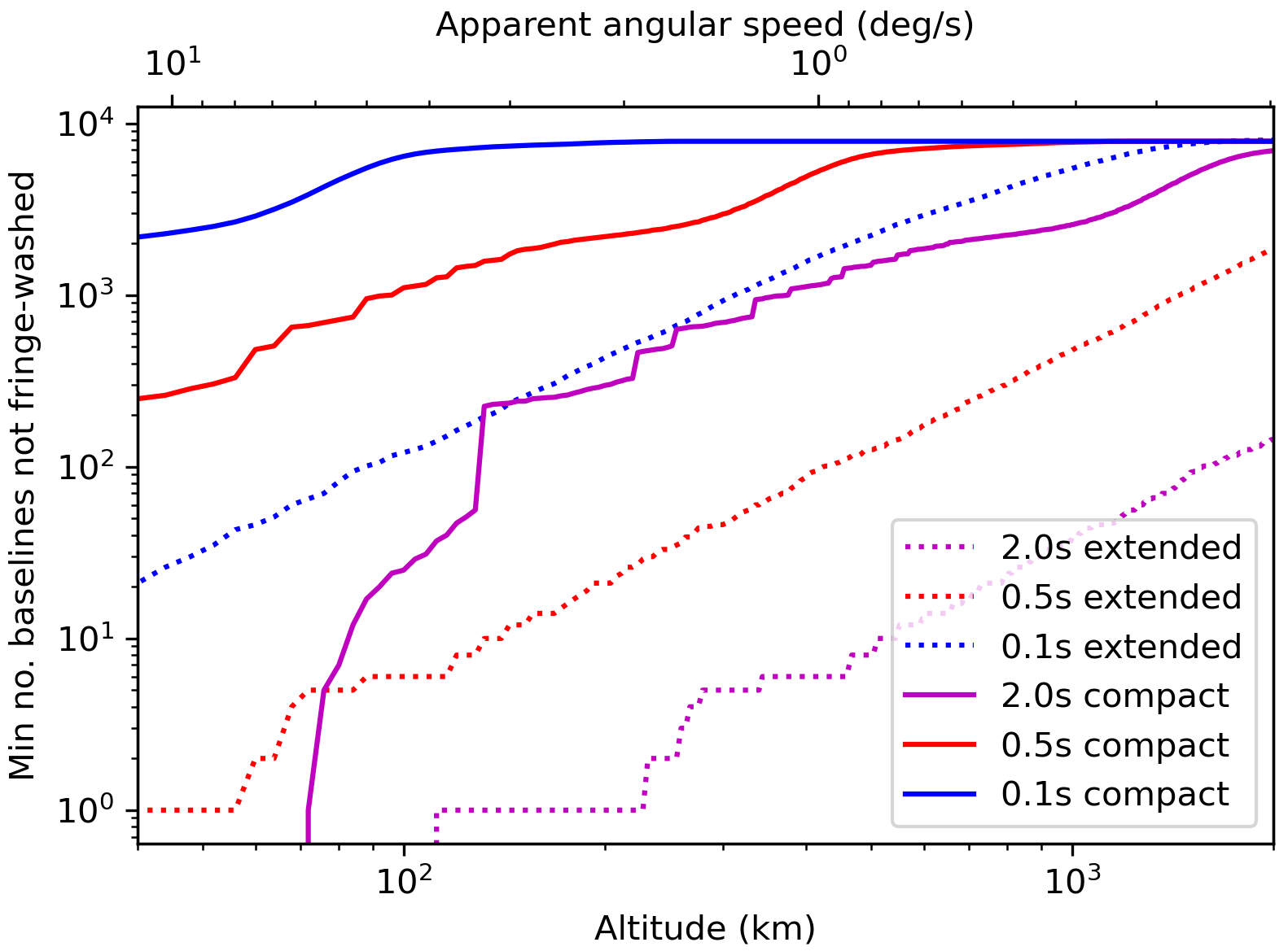
Figure 10: The minimum number of baselines not fringe-washed as a function of satellite altitude (or angular speed). The actual number of baselines not affected depends on the direction of the satellite pass (as baselines perpendicular to the satellite motion are not fringe-washed).

4 CONCLUSION

In this paper we have developed and demonstrated two different methods to improve the detection sensitivity of the non-coherent MWA SDA system. The first RSO search method is called shift-stacking. The method increases the SNR of faint RSO signals by averaging the signal along the predicted trajectory, through coherent stacking. We test the method for all the objects that passed through the MWA’s primary beam during the $20$ hours of observation used during our previous blind survey [20]. The shift-stacking targeted search resulted in $55$ new detections that were previously not detected by our blind detection pipeline, demonstrating that the shift-stacking method is able to probe a weaker population of signals as it uses prior information about the object’s pass to perform signal stacking. The MWA shift-stacking pipeline also identifies the in-track and cross-track offsets of the RSO detections, and these measurements can be used to perform RSO catalog updates.

The second method performs detections of weak RSO signals by re-focusing the interferometer to the desired near-field RSO location. It does so by calculating the apparent delay as seen by a baseline and converting it into a visibility phase correction. This method was proved to work effectively using an extended array observation of the ISS. The previously undetected ISS FM reflection signal in the long-baseline difference image of the observation was recovered after applying the required near-field phase correction. However, the recovered signal was weaker than expected, due to visibility fringe-washing. The phase of the ISS signal changed rapidly (during the correlator integration time of $0.5$ s) resulting in de-correlation of the signal. However, with the ongoing upgrade of MWA to Phase 3, we should be able to perform more sensitive near-field detections due to being able to sample the apparent sky with $0.1$ s averaging (reduces fringe-washing).

In summary, the implementation of the shift-stack method has increased the detection rate of the non-coherent MWA SDA system by $75\%$. Any future SDA dedicated arrays that may be built using MWA-like technology should incorporate short baselines to avoid fringe-washing of RSO signals or incorporate correlators that allow smaller integration times (higher data rate), due to the issues discussed in this paper. In the future, the near-field phase correction software developed can be modified to determine the 3D location of the target by iterative maximisation of the RSO signal, by varying its predicted location (the SNR of the focused signal is maximum when the predicted near-field location matches with its true position).

Sofware

We acknowledge the work and the support of the developers of the following Python packages: Astropy [24, 1], Numpy [29], Scipy [9], matplotlib [7], seaborn python-casacore ,and SkyField. The work also used WSCLEAN [16, 17] for making fits images and DS9 for visualization purposes. Adobe Illustrator was used for creating Figure 2.

Appendix A Visibility fringe-washing as a function of satellite altitude

The classical mechanics equation for the linear velocity of a satellite in a circular orbit around Earth is given by

$$\begin{array}[]{l}v=\sqrt{\frac{\displaystyle GM}{\displaystyle R+alt}}\par\par\end{array}$$ (4)

where $v$ ($m/s$) is the linear velocity of the satellite, $G$ is the gravitational constant ($6.67408\times 10^{-11}m^{3}kg^{-1}s^{-2}$), $R$ ($6.371\times 10^{6}$ m) is the radius of Earth, $M$ is the mass of Earth ($5.972\times 10^{24}$ kg) and $alt$ is the altitude of the considered satellite.

The fringe-rate (the time rate of change of the visibility phase) as measured by a zenith pointed East-West baseline is given by (obtained from [12])

$$\begin{array}[]{l}\frac{\displaystyle\delta\Phi}{\displaystyle\delta t}\approx 2\pi\omega\frac{\displaystyle b}{\displaystyle\lambda}\end{array}$$ (5)

and for small integration times Equation 5 becomes

$$\begin{array}[]{l}\frac{\displaystyle\Delta\Phi}{\displaystyle\Delta t}\approx 2\pi\omega\frac{\displaystyle b}{\displaystyle\lambda}\\ \end{array}$$ (6)

$$\begin{array}[]{l}\Delta\Phi\approx 2\pi\omega\frac{\displaystyle b}{\displaystyle\lambda}\Delta t\end{array}$$ (7)

For an observer on the surface (i.e, the MWA), the apparent angular motion (for small angles near the zenith) can be derived using the derivative form of $s=r\theta$ relating angular velocity with linear velocity ($v=r\omega$). The apparent angular velocity $\omega$ for a satellite (near the zenith) can be determined using Equation 4

$$\begin{array}[]{l}\omega=\frac{\displaystyle v}{\displaystyle radius}=\frac{\displaystyle v}{\displaystyle alt}\\ \implies\quad\omega=\frac{\displaystyle 1}{\displaystyle alt}\sqrt{\frac{\displaystyle GM}{\displaystyle R+alt}}\par\end{array}$$ (8)

Substituting the value of $\omega$ from Equation 8 in Equation 6, we get the function relating the change in visibility phase as measured by a baseline for the apparent motion of a satellite.

$$\begin{array}[]{l}\Delta\Phi\approx 2\pi\frac{\displaystyle b}{\displaystyle\lambda\times alt}\sqrt{\frac{\displaystyle GM}{\displaystyle R+alt}}\Delta t\par\par\end{array}$$ (9)

Appendix B List of new detections

Table 1: All the new events detected by the shift-stacking targeted search. We list the North American Aerospace Defence (NORAD) catalog number of all the objects detected along with its RCS, shortest range during observation, and its apparent peak flux density.

Observation	Name	Norad ID	RCS	Shortest Range	Apparent Peak Flux Density
ID			$m^{2}$	km	(Jy/beam)
1165782736	DELTA 2 R/B(1)	24809	9.88	668	5.41
1165782496	DELTA 2 R/B(1)	23640	9.75	954	5.65
1165776496	CZ-2D R/B	36597	8.72	582	6.09
1165776256	SL-24 R/B	31123	5.23	811	7.85
1165775896	FENGYUN 3B	37214	6.21	863	7.43
1165771576	SUOMI NPP	37849	5.78	848	8.78
1165770376	IRIDIUM 43	25039	3.20	788	5.18
1165770256	ATLAS AGENA D R/B	2144	6.04	761	5.32
1165768576	ASTRO-H (HITOMI)	41337	6.16	603	7.11
1165767376	OCEANSAT-2	35931	4.06	732	6.14
1165766296	SL-16 R/B	24298	8.49	871	6.79
1165765936	OAO 1	2142	12.1	807	4.33
1165765816	PSLV R/B	25759	6.06	737	5.20
1165763536	DELTA 2 DEB [DPAF]	29110	5.07	662	4.61
1165763536	KAZEOSAT 1	39731	4.22	765	3.66
1165760896	COSMOS 2486	39177	16.0	741	2.18
1165759696	KORONAS-FOTON	33504	4.18	524	6.90
1165757896	KMS 4	41332	0.61	475	3.29
1165757056	CZ-2C DEB	40288	0.08	793	2.86
1165753576	CAMEO and DELTA 1 R/B	11081	8.30	975	6.23
1160505712	IRIDIUM 7	24793	3.32	799	5.72
1160505112	IRIDIUM 6	24794	3.23	794	8.27
1160504872	SL-24 DEB	33318	4.64	593	6.12
1160504272	SL-16 R/B	17974	9.05	858	10.0
1160503672	IRS-1D	24971	3.91	760	9.29
1160502232	FORTE	24920	1.35	809	6.57
1160500192	SL-14 R/B	10974	4.12	619	4.62
1160499712	SUZAKU (ASTRO-EII)	28773	4.15	538	7.94
1160499352	INTERCOSMOS 25	21819	7.32	688	8.92
1160498872	CZ-2C R/B	40262	7.47	690	10.5
1160489992	PSLV R/B	41620	6.71	485	9.66
1160489152	METOP-B	38771	13.6	840	6.87
1160489032	H-2A R/B	38341	17.2	655	6.57
1160483992	COSMOS 1833	17589	4.11	841	7.97
1160482912	FENGYUN 3A	32958	6.58	845	9.37
1160479912	COSMOS 1300	12785	5.69	531	16.2
1157489632	SL-24 R/B	31699	5.92	557	21.3
1157469232	KORONAS-FOTON	33504	4.18	554	17.9
1157459032	ALOS (DAICHI)	28931	13.6	700	33.5
1157406472	SL-14 R/B	14820	3.82	623	4.42
1157406472	TSX-5	26374	1.84	919	3.42
1157401672	SL-3 R/B	7275	6.37	889	6.34
1157398072	BREEZE-M DEB [TANK]	36594	6.29	825	4.05
1157384272	SJ-11-07	40261	2.26	712	8.18
1157378272	METOP-A	29499	11.2	830	8.86
1165769776	COSMOS 860	9486	2.28	1015	4.71
1160496712	SL-12 R/B(2)	27473	20.3	1329	3.73
1160495392	YAOGAN 25A	40338	2.33	1074	5.19

Continued on next page…

Table 1: …continued from previous page.

Observation	Name	Norad ID	RCS	Shortest Range	Apparent Peak Flux Density
ID			$m^{2}$	km	(Jy/beam)
1160495392	YAOGAN 25C	40340	2.63	1066	6.21
1160495392	YAOGAN 25B	40339	2.39	1075	3.09
1157484832	CZ-3 R/B	20474	9.30	1014	26.3
1165762936	CBERS 4	40336	3.78	783	6.94
1160498512	SL-8 R/B	11170	6.04	1187	5.08
1160491312	SL-24 DEB	35689	4.88	649	8.64
1160492992	DELTA 1 R/B(1)	10793	9.06	627	10.8

References

- [1] Astropy Collaboration, A.. Price-Whelan and B.. Sipőcz “The Astropy Project: Building an Open-Science Project and Status of the v2.0 Core Package” In The Astronomical Journal 156, 2018, pp. 123 DOI: 10.3847/1538-3881/aabc4f
- [2] G.. Bernstein et al. “The Size Distribution of Trans-Neptunian Bodies” In AJ 128.3, 2004, pp. 1364–1390 DOI: 10.1086/422919
- [3] N. Bobrinsky and L. Del Monte “The space situational awareness program of the European Space Agency” In Cosmic Research 48.5, 2010, pp. 392–398 DOI: 10.1134/S0010952510050035
- [4] Luke D. Burkhart, Darin Ragozzine and Michael E. Brown “A Deep Search for Additional Satellites around the Dwarf Planet Haumea” In AJ 151.6, 2016, pp. 162 DOI: 10.3847/0004-6256/151/6/162
- [5] B. Hennessy et al. “Improved Techniques for the Surveillance of the Near Earth Space Environment with the Murchison Widefield Array” In 2019 IEEE Radar Conference (RadarConf), 2019, pp. 1–6 DOI: 10.1109/RADAR.2019.8835821
- [6] Brendan Hennessy, Mark Rutten, Steven Tingay and Robert Young “Orbit Determination Before Detect: Orbital Parameter Matched Filtering for Uncued Detection” In 2020 IEEE International Radar Conference (RADAR), 2020, pp. 889–894 IEEE
- [7] J.. Hunter “Matplotlib: A 2D graphics environment” In Computing in Science & Engineering 9.3 IEEE COMPUTER SOC, 2007, pp. 90–95 DOI: 10.1109/MCSE.2007.55
- [8] N. Hurley-Walker et al. “GaLactic and Extragalactic All-sky Murchison Widefield Array (GLEAM) survey - I. A low-frequency extragalactic catalogue” In MNRAS 464.1, 2017, pp. 1146–1167 DOI: 10.1093/mnras/stw2337
- [9] Eric Jones, Travis Oliphant and Pearu Peterson “SciPy: Open Source Scientific Tools for Python”, 2001
- [10] D.. Kessler and B.. Cour-Palais “Collision frequency of artificial satellites: The creation of a debris belt” In J. Geophys. Res. 83, 1978, pp. 2637–2646 DOI: 10.1029/JA083iA06p02637
- [11] Bhavya Lal et al. “Global trends in space situational awareness (SSA) and space traffic management (STM)”, 2018
- [12] Jonathan M Marr, Ronald L Snell and Stanley E Kurtz “Fundamentals of radio astronomy: observational methods” CRC Press, 2015
- [13] J.. McMullin et al. “CASA Architecture and Applications” In Astronomical Data Analysis Software and Systems XVI 376, Astronomical Society of the Pacific Conference Series, 2007, pp. 127
- [14] James G Miller “A new sensor allocation algorithm for the space surveillance network” In Military Operations Research JSTOR, 2007, pp. 57–70
- [15] Giacomo Muntoni “Crowded Space: A Review on Radar Measurements for Space Debris Monitoring and Tracking” In Applied Sciences 11.4, 2021, pp. 1364 DOI: 10.3390/app11041364
- [16] A.. Offringa, B. McKinley and Hurley-Walker “WSClean: an implementation of a fast, generic wide-field imager for radio astronomy” In MNRAS 444.1, 2014, pp. 606–619 DOI: 10.1093/mnras/stu1368
- [17] A.. Offringa and O. Smirnov “An optimized algorithm for multiscale wideband deconvolution of radio astronomical images” In MNRAS 471.1, 2017, pp. 301–316 DOI: 10.1093/mnras/stx1547
- [18] A.. Offringa et al. “Parametrizing Epoch of Reionization foregrounds: a deep survey of low-frequency point-source spectra with the Murchison Widefield Array” In MNRAS 458.1, 2016, pp. 1057–1070 DOI: 10.1093/mnras/stw310
- [19] James E. Palmer et al. “Surveillance of Space using Passive Radar and the Murchison Widefield Array” In arXiv e-prints, 2019, pp. arXiv:1910.04435 arXiv:1910.04435 [eess.SP]
- [20] S. Prabu, P. Hancock, X. Zhang and S.. Tingay “A low-frequency blind survey of the low Earth orbit environment using non-coherent passive radar with the Murchison widefield array” In Publications of the Astronomical Society of Australia 37 Cambridge University Press, 2020, pp. e052 DOI: 10.1017/pasa.2020.40
- [21] Steve Prabu, Paul J. Hancock, Xiang Zhang and Steven J. Tingay “The development of non-coherent passive radar techniques for space situational awareness with the Murchison Widefield Array” In Publications of the Astronomical Society of Australia 37 Cambridge University Press, 2020, pp. e010 DOI: 10.1017/pasa.2020.1
- [22] Malena Rice and Gregory Laughlin “Exploring Trans-Neptunian Space with TESS: A Targeted Shift-stacking Search for Planet Nine and Distant TNOs in the Galactic Plane” In The Planetary Science Journal 1.3, 2020, pp. 81 DOI: 10.3847/PSJ/abc42c
- [23] Makoto Tagawa et al. “Orbital objects detection algorithm using faint streaks” In Advances in Space Research 57.4 Elsevier, 2016, pp. 929–937
- [24] The Astropy Collaboration, Thomas P. Robitaille and Erik J. Tollerud “Astropy: A Community Python Package for Astronomy” In Astronomy & Astrophysics 558, 2013, pp. 9–9 DOI: 10.1051/0004-6361/201322068
- [25] S.. Tingay et al. “The murchison widefield array: The square kilometre array precursor at low radio frequencies” In Publications of the Astronomical Society of Australia 30.1, 2013 DOI: 10.1017/pasa.2012.007
- [26] S.. Tingay et al. “On the detection and tracking of space debris using the murchison widefield array. I. Simulations and test observations demonstrate feasibility” In Astronomical Journal 146.4, 2013 DOI: 10.1088/0004-6256/146/4/103
- [27] S.. Tingay, M. Sokolowski, R. Wayth and D. Ung “A survey of spatially and temporally resolved radio frequency interference in the FM band at the Murchison Radio-astronomy Observatory” In PASA 37, 2020, pp. e039 DOI: 10.1017/pasa.2020.32
- [28] S.. Tremblay et al. “The High Time and Frequency Resolution Capabilities of the Murchison Widefield Array” In PASA 32, 2015, pp. e005 DOI: 10.1017/pasa.2015.6
- [29] Stéfan van der Walt, S Chris Colbert and Gaël Varoquaux “The NumPy Array: A Structure for Efficient Numerical Computation” In Computing in Science & Engineering 13.2, 2011, pp. 22–30 DOI: 10.1109/MCSE.2011.37
- [30] R.. Wayth et al. “The Phase II Murchison Widefield Array: Design overview” In PASA 35, 2018 DOI: 10.1017/pasa.2018.37
- [31] Xiang Zhang et al. “Limits on radio emission from meteors using the MWA” In Monthly Notices of the Royal Astronomical Society 11.April, 2018, pp. 1–11 DOI: 10.1093/mnras/sty930