Quasi-static decomposition and the Gibbs factorial in small thermodynamic systems

Abstract

For small thermodynamic systems in contact with a heat bath, we determine the free energy by imposing the following two conditions. First, the quasi-static work in any configuration change is equal to the free energy difference. Second, the temperature dependence of the free energy satisfies the Gibbs-Helmholtz relation. We find that these prerequisites uniquely lead to the free energy of a classical system consisting of $N$-interacting identical particles, up to an additive constant proportional to $N$. The free energy thus determined contains the Gibbs factorial $N!$ in addition to the phase space integration of the Gibbs-Boltzmann factor. The key step in the derivation is to construct a quasi-static decomposition of small thermodynamic systems.

1 Introduction

Suppose that a small thermodynamic system contacts with a heat bath of temperature $T$. For equilibrium cases, microscopic states obey a canonical distribution. Dynamical properties of the system are described by stochastic processes with the detailed balance condition or by projected dynamics of the system from the Hamiltonian dynamics of the total system containing the heat bath. The transition from an equilibrium state to another equilibrium state is caused by a time-dependent parameter. Even for small systems without the thermodynamic limit, thermodynamic concepts such as the first law and the second law are formulated together with incorporating fluctuation properties Sekimoto ; Seifert ; Peliti .

We study $N$-interacting identical particles whose Hamiltonian is given by $H(\Gamma;{\cal C})$ with a microscopic coordinate $\Gamma$ and a set of parameters ${\cal C}$ describing a system configuration. The equilibrium state is given by the canonical distribution

$$\rho_{\beta}(\Gamma;{\cal C})=\frac{1}{Z(T,{\cal C})}\exp(-\beta H(\Gamma;{\cal C})),$$ (1)

where $\beta\equiv 1/(k_{\rm B}T)$ with the Boltzmann constant $k_{\rm B}$ and the partition function $Z(T,{\cal C})$ is given by

$$Z(T,{\cal C})=\int d\Gamma\exp(-\beta H(\Gamma;{\cal C}))$$ (2)

from the normalization condition $\int d\Gamma\rho_{\beta}(\Gamma;{\cal C})=1$. We then define the free energy $F(T,{\cal C})$ of this system from the following two prerequisites. First, for any ${\cal C}_{0}$ and ${\cal C}_{1}$, the free energy difference $F(T,{\cal C}_{1})-F(T,{\cal C}_{0})$ is equal to the quasi-static work from ${\cal C}_{0}$ to ${\cal C}_{1}$. Because the latter is expressed by the partition function, the first condition is expressed as

$$F(T,{\cal C}_{1})-F(T,{\cal C}_{0})=-k_{\rm B}T[\log Z(T,{\cal C}_{1})-\log Z(T,{\cal C}_{0})].$$ (3)

See Sec. 2.2 for the derivation. The second condition is that $F(T,{\cal C})$ satisfies the Gibbs-Helmholtz relation:

$$E=\frac{\partial(\beta F)}{\partial\beta},$$ (4)

where $E$ is the expectation of $H(\Gamma;{\cal C})$.

As the simplest configuration, we consider the case where $N$-interacting identical particles are confined in a cuboid container of volume $V$. The partition function and the free energy of this system are denoted by $Z(T,V,N)$ and $F(T,V,N)$. It has been known that (3) and (4) lead to

$$F(T,V,N)=-k_{\rm B}T[\log Z(T,V,N)-\bar{\phi}(N)]$$ (5)

with a function $\bar{\phi}(N)$. See Sec. 2.2 for a review of the derivation. Then, the main claim of this paper is that we can derive

$$\bar{\phi}(N)=\log N!+c_{0}N$$ (6)

from (3), where $c_{0}$ is an arbitrary constant. Substituting (6) into (5), we obtain

$$F(T,V,N)=-k_{\rm B}T\left[\log\frac{Z(T,V,N)}{N!}-c_{0}N\right].$$ (7)

The formula (7) has been explained in standard textbooks of statistical mechanics. If the system is described by quantum mechanics, the free energy is defined as

$$F\equiv{\rm Tr}[\hat{\rho}_{\beta}\hat{H}]+k_{\rm B}T{\rm Tr}[\hat{\rho}_{\beta}\log\hat{\rho}_{\beta}]$$ (8)

using the density matrix $\hat{\rho}_{\beta}({\cal C})$ with a Hamiltonian $\hat{H}({\cal C})$. For $N$-interacting identical particles, the classical limit of $F$ leads to (7) with $c_{0}=3\log h$, where $h$ is the Planck constant. However, when $\hat{\rho}_{\beta}$ and $\hat{H}$ in (8) are replaced by $\rho_{\beta}(\Gamma;{\cal C})$ and $H(\Gamma;{\cal C})$, (8) becomes (7) without $N!$. From this fact, one may understand that $N!$, which we call the Gibbs factorial, comes from quantum mechanics. However, this interpretation is not logically correct, because it might be possible that the definition of $F$ in (8) is not valid. There are several approaches characterizing the Gibbs factorial in classical systems Kampen ; Jaynes ; Warren ; Swedsen ; Frenkel ; Murashita ; Yoshida . Our argument stands on a general principle that thermodynamic quantities are defined by experimentally measurable quantities. That is, whether or not $N!$ appears in the formula should be determined by thermodynamic considerations. This viewpoint has been repeatedly explained in the literature Kampen ; Jaynes .

To determine the functional form of $\bar{\phi}(N)$ based on (3), one may conjecture that a quasi-static decomposition process can be achieved by inserting a separating wall slowly. If the decomposition were possible without work as assumed in macroscopic thermodynamics, (3) could lead to

$$F(T,\lambda V,\lambda N)+F(T,(1-\lambda)V,(1-\lambda)N)-F(T,V,N)=0$$ (9)

for any $N$ and $\lambda$ such that $\lambda N$ is an integer. The combination of (5) with (9) gives

$$\bar{\phi}(N)=N\log N+c_{1}N,$$ (10)

as shown in Sec. 2.3, where $c_{1}$ is an arbitrary constant. Here, (10) is consistent with (6) when $o(N)$ terms are ignored in the thermodynamic limit $N\to\infty$ and $V\to\infty$ with $V/N$ fixed, while (10) is not equal to (6) for finite $N$ cases. The correct statement is that (9) is valid only in the thermodynamic limit. Thus, the Gibbs factorial $N!$ for macroscopic systems is understood by thermodynamic considerations, but (6) has not been derived from (3) for finite $N$ cases.

The difference between (6) and (10) has been studied from the viewpoint of information thermodynamics Yoshida . Indeed, one can quickly insert a separating wall after measuring the particle number in the left region of the volume $\lambda V$. Then, the free energy associated with measurement-and-feedback appears on the right-hand side of (9). The form of $\bar{\phi}(N)$, taking account of this contribution, is found to be (6), not (10). This argument provides the operational foundation of (7). Therefore, the Gibbs factorial $N!$ would be derived only from quasi-static works if the quasi-static process corresponding to the free energy obtained by measurement-and-feedback is constructed.

Concerning the last point, in Ref. Horowitz , it is claimed that such a quasi-static process exists, but the process is not explicitly shown. In the present paper, we construct a quasi-static decomposition process using a special confining potential.

Here, it should be noted that for a system consisting of identical particles, the symmetry of the Hamiltonian for any permutation of particle indexes plays an essential role in the calculation of the quasi-static work. In contrast, when two types of particles, A and B, are mixed, the Gibbs factorial becomes $N_{A}!N_{B}!$, where $N_{A}$ and $N_{B}$ are the numbers of particles of type $A$ and $B$, respectively. In addition to the quasi-static decomposition, the separation of different types of particles is conducted using a semi-permeable wall under the assumption that the semi-permeable wall can be prepared for any type described in the Hamiltonian.

The remainder of the paper is organized as follows. In Sec. 2, we describe the setup of our study. We then derive (3), (5), and (10) as a review. In Sec. 3, we derive the main result (6). In Sec. 4, we study binary mixtures and clarify how the Gibbs factorial is modified from simple systems. In Sec. 5, we briefly comment on the other approaches presented in Refs. Warren ; Swedsen ; Frenkel ; Murashita . We also consider quantum systems from the viewpoint of quasi-static decomposition.

2 Preliminaries

2.1 Setup

We study $N$-interacting particles confined in a cuboid region $D$ with $|D|=V$, where $|D|$ represents the volume of of the region $D$. Let $({\bm{r}}_{i},{\bm{p}}_{i})\in\mathbb{R}^{6}$ be the position and momentum of $i$-th particle. The phase space coordinate $\Gamma$ of the system is then given by

$$\Gamma=({\bm{r}}_{1},{\bm{r}}_{2},\cdots,{\bm{r}}_{N},{\bm{p}}_{1},{\bm{p}}_{2},\cdots,{\bm{p}}_{N}).$$ (11)

We assume the Hamiltonian of the system as

$$H_{0}(\Gamma)=\sum_{i=1}^{N}\frac{|{\bm{p}}_{i}|^{2}}{2m}+\sum_{i<j}V_{\rm int}(|{\bm{r}}_{i}-{\bm{r}}_{j}|),$$ (12)

where $V_{\rm int}$ represents a short-range interaction between two particles. For simplicity, we assume that there exists a microscopic length $\xi$ such that $V_{\rm int}(r)=0$ for $r\geq\xi$.

To describe confinement of the $N$ particles into the region $D$, we introduce a wall potential

$$V_{\rm wall}({\bm{r}};D,\kappa)=\frac{\kappa}{2}|d({\bm{r}},D)|^{2}$$ (13)

with

$$d({\bm{r}},D)=\inf_{{\bm{r}}^{\prime}\in D}|{\bm{r}}-{\bm{r}}^{\prime}|,$$ (14)

which indicates the distance between a point ${\bm{r}}$ and the region $D$. The parameter $\kappa$ in (13) represents the strength of confinement. We express the total Hamiltonian as

$$H(\Gamma;D,\kappa)=H_{0}(\Gamma)+\sum_{i=1}^{N}V_{\rm wall}({\bm{r}}_{i};D,\kappa).$$ (15)

The canonical distribution for this Hamiltonian is given by

$$\rho_{\beta}(\Gamma;D,\kappa)=\frac{1}{Z(T,V,N;\kappa)}\exp(-\beta H(\Gamma;D,\kappa))$$ (16)

with the partition function

$$Z(T,V,N;\kappa)=\int d\Gamma\exp(-\beta H(\Gamma;D,\kappa)),$$ (17)

where only $V$ dependence of $Z$ is explicitly written in the $D$ dependence of $Z$. In the hard wall limit $\kappa\to\infty$, we have the standard partition function

$$Z(T,V,N) =\lim_{\kappa\to\infty}Z(T,V,N;\kappa),$$ (18)

$$=\int d\Gamma\exp(-\beta H_{0}(\Gamma))\prod_{i=1}^{N}\chi({\bm{r}}_{i}\in D),$$ (19)

where $\chi({\cal A})=1$ if ${\cal A}$ is true, otherwise $\chi({\cal A})=0$.

More generally, $V_{\rm con}(\Gamma;{\cal C})$ denotes a general confining potential described by a set of parameters ${\cal C}$. We then write

$$H(\Gamma;{\cal C})=H_{0}(\Gamma)+V_{\rm con}(\Gamma;{\cal C}).$$ (20)

The canonical distribution and the partition function of this system are given by (1) and (2). Thermodynamic processes are described by time-dependence of ${\cal C}$ that describes a system configuration. In particular, for any ${\cal C}_{0}$ and ${\cal C}_{1}$, a quasi-static process connecting them is represented by a one-parameter continuous family ${\cal C}_{\alpha}$, where $0\leq\alpha\leq 1$, which forms a path in the parameter space. The quasi-static work done in this process is defined by

$$W({\cal C}_{0}\to{\cal C}_{1})=\int_{0}^{1}d\alpha\int d\Gamma\rho_{\beta}(\Gamma;{\cal C}_{\alpha})\frac{\partial H(\Gamma;{\cal C}_{\alpha})}{\partial\alpha}.$$ (21)

2.2 Derivation of (3) and (5)

We substitute (1) into the right-hand side of (21), and then calculate it as

$$W({\cal C}_{0}\to{\cal C}_{1}) =-k_{\rm B}T\int_{0}^{1}d\alpha\frac{1}{Z(T;{\cal C}_{\alpha})}\int d\Gamma\frac{\partial}{\partial\alpha}\exp(-\beta H(\Gamma;{\cal C}_{\alpha}))$$

$$=-k_{\rm B}T\int_{0}^{1}d\alpha\frac{\partial}{\partial\alpha}\log Z(T;{\cal C}_{\alpha})$$

$$=-k_{\rm B}T[\log Z(T;{\cal C}_{1})-\log Z(T;{\cal C}_{0})].$$ (22)

From the condition that the free energy difference is equal to $W({\cal C}_{0}\to{\cal C}_{1})$, we obtain (3).

As a special case, we consider the system with a confining potential

$$V_{\rm con}(\Gamma;{\cal C})=\sum_{i=1}^{N}V_{\rm wall}({\bm{r}}_{i};D).$$ (23)

Let $F(T,V,N;\kappa)$ be the free energy of the system. The formula (3) in this case becomes

$$F(T,V_{1},N;\kappa)-F(T,V_{0},N;\kappa)=-k_{\rm B}T[\log Z(T,V_{1},N;\kappa)-\log Z(T,V_{0},N;\kappa)]$$ (24)

for any $V_{0}$ and $V_{1}$. Taking the limit $\kappa\to\infty$, we obtain

$$F(T,V_{1},N)-F(T,V_{0},N)=-k_{\rm B}T[\log Z(T,V_{1},N)-\log Z(T,V_{0},N)].$$ (25)

Note that the formula (3) cannot be directly applied to the system with $\kappa\to\infty$ because $\partial H/\partial\alpha$ is not defined for the case $\kappa\to\infty$. This is the reason why we need to pass (24) to get (25). Because the relation (25) holds for any $V_{0}$ and $V_{1}$, $F(T,V,N)$ takes the form

$$F(T,V,N)=-k_{\rm B}T\log Z(T,V,N)+\phi(T,N),$$ (26)

where a functional form of $\phi(T,N)$ is not determined yet.

Furthermore, the expectation of the energy is calculated as

$$E=-\frac{\partial\log Z}{\partial\beta}.$$ (27)

The condition (4) is then expressed as

$$\frac{\partial(\beta F+\log Z)}{\partial\beta}=0.$$ (28)

This equality with (26) becomes

$$\frac{\partial\beta\phi(T,N)}{\partial\beta}=0,$$ (29)

which leads to

$$\phi(T,N)=k_{\rm B}T\bar{\phi}(N)$$ (30)

with a function $\bar{\phi}(N)$. Substituting (30) into (26), we obtain (5).

2.3 Derivation of (10)

Let $H_{\rm id}(\Gamma;D,\kappa)$ be the Hamiltonian of $N$-free particles confined in the same region $D$. The system corresponds to the ideal gas in thermodynamics. The partition function of the system is denoted by $Z_{\rm id}(T,V,N)$. Here, putting $\alpha$ in front of $V_{\rm int}$ in (12), we change $\alpha$ from $\alpha=0$ to $\alpha=1$ gradually. We then have a quasi-static process from $H_{\rm id}(\Gamma;D,\kappa)$ to $H(\Gamma;D,\kappa)$. Because the work done in the quasi-static process is equal to the free energy difference of the two systems, the relation

$$F(T,V,N)-F_{\rm id}(T,V,N)=-k_{\rm B}T[\log Z(T,V,N)-\log Z_{\rm id}(T,V,N)]$$ (31)

holds. By substituting (5) into (31), we obtain

$$F_{\rm id}(T,V,N)=-k_{\rm B}T[\log Z_{\rm id}(T,V,N)-\bar{\phi}(N)].$$ (32)

This expression indicates that $\bar{\phi}(N)$ is independent of $H_{0}(\Gamma)$. Now, we can directly calculate $Z_{\rm id}(T,V,N)$ as

$$Z_{\rm id}(T,V,N)=\left(\frac{2m\pi}{\beta}\right)^{3N/2}V^{N}.$$ (33)

We substitute (32) with (33) into (9) for $F_{\rm id}$. We then have

$$\bar{\phi}(\lambda N)+\bar{\phi}((1-\lambda)N)-\bar{\phi}(N)=N[\lambda\log\lambda+(1-\lambda)\log(1-\lambda)].$$ (34)

Because this relation holds for any $N$ and $\lambda$ such that $\lambda N$ is an integer, we obtain (10).

3 Derivation of the main result (6)

3.1 Outline

The key step in the derivation of (6) is to construct a quasi-static decomposition. We start with a description of the decomposed system. Let $D^{\rm L}$ and $D^{\rm R}$ be two cuboid regions separated by greater than the interaction length $\xi$. By using a confining potential with a strength $\kappa$, we attempt to construct a system where $N^{\rm L}$ and $N^{\rm R}$ particles are almost in $D^{\rm L}$ and $D^{\rm R}$, where $N^{\rm L}+N^{\rm R}=N$ and $|D^{\rm L}|=V^{\rm L}$ and $|D^{\rm R}|=V^{\rm R}=V-V^{\rm L}$. Let ${\cal C}_{1}$ be a parameter set of the confining potential for the decomposed system, and ${\cal C}_{0}$ be the confining potential given in (23). The most important step is to find a continuous family of confining potentials $V_{\rm con}(\Gamma;{\cal C}_{\alpha})$ with $0\leq\alpha\leq 1$ starting from (23). Here, it is assumed that a particular $N^{\rm L}$-particles cannot be selected by controlling a potential without measuring particle positions. This property is expressed by

$$V_{\rm con}(\Gamma_{\sigma};{\cal C}_{\alpha})=V_{\rm con}(\Gamma;{\cal C}_{\alpha})$$ (35)

with

$$\Gamma_{\sigma}\equiv({\bm{r}}_{\sigma(1)},{\bm{r}}_{\sigma(2)},\cdots,{\bm{r}}_{\sigma(N)},{\bm{p}}_{\sigma(1)},{\bm{p}}_{\sigma(2)},\cdots,{\bm{p}}_{\sigma(N)})$$ (36)

for any $\Gamma$ and $\sigma\in P$, where $P$ denotes a set of all permutations of $\{1,2,\cdots,N\}$. If such a family of potentials $V_{\rm con}(\Gamma;{\cal C}_{\alpha})$, $0\leq\alpha\leq 1$, is found, (3) can be applied to the quasi-static decomposition process represented by this $({\cal C}_{\alpha})_{\alpha=0}^{1}$. Then, we take the limit $\kappa\to\infty$ for the obtained expression. The result is

$$F(T,V^{\rm L},N^{\rm L})+F(T,V^{\rm R},N^{\rm R})-F(T,V,N)=-k_{\rm B}T\lim_{\kappa\to\infty}[\log Z(T,{\cal C}_{1})-\log Z(T,{\cal C}_{0})],$$ (37)

where the numbers of particles in the regions $D^{\rm L}$ and $D^{\rm R}$ are fixed as $N^{\rm L}$ and $N^{\rm R}$. Because

$$Z(T,{\cal C}_{0})=Z(T,V,N;\kappa),$$ (38)

we have only to calculate $\log Z(T,{\cal C}_{1})$. In the next section, by explicitly constructing the quasi-static decomposition, we calculate

$$\lim_{\kappa\to\infty}Z(T,{\cal C}_{1})=\frac{N!}{N^{\rm L}!N^{\rm R}!}Z(T,V^{\rm L},N^{\rm L})Z(T,V^{\rm R},N^{\rm R}).$$ (39)

Substituting (5), (38), and (39) into (37), we obtain

$$\phi(N^{\rm L})+\phi(N^{\rm R})-\phi(N)+\log\frac{N!}{N^{\rm L}!N^{\rm R}!}=0.$$ (40)

Because this holds for any $N$, $N^{\rm L}$, and $N^{\rm R}$, we conclude (6).

3.2 Derivation of (39)

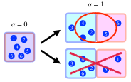
Figure 1: Illustration of a decomposed system using the confining potential (41). $N=6$, $N^{\rm L}=4$, and $N^{\rm R}=2$. Because particles with index $i$ satisfying $1\leq i\leq N^{\rm L}$ are distinguished from the others, this operation is not allowed.

We explicitly construct a confining potential for the decomposed system described by ${\cal C}_{1}$, where $N^{\rm L}$ and $N^{\rm R}$ particles are almost in $D^{\rm L}$ and $D^{\rm R}$. One may naively consider such a potential as

$$V_{\rm con}(\Gamma;{\cal C}_{1})=\sum_{i=1}^{N^{\rm L}}V_{\rm wall}({\bm{r}}_{i};D^{\rm L})+\sum_{i=N^{\rm L}+1}^{N}V_{\rm wall}({\bm{r}}_{i};D^{\rm R}),$$ (41)

illustrated in Fig. 1. The confining potential (41) does not satisfy (35) with $\alpha=1$. This means that if (41) were realized in a quasi-static process from (23), particles with index $i$ satisfying $1\leq i\leq N^{\rm L}$ could be distinguished from the others. However, such distinguishment of identical particles is not allowed in the operation. Therefore, we have to look for a potential that is symmetric with respect to permutations of particle indexes.

As such an example, we propose

$$V_{\rm con}(\Gamma;{\cal C}_{1})\equiv\min_{\sigma\in P}\left[\sum_{i=1}^{N^{\rm L}}V_{\rm wall}({\bm{r}}_{\sigma(i)};D^{\rm L})+\sum_{i=N^{\rm L}+1}^{N}V_{\rm wall}({\bm{r}}_{\sigma(i)};D^{\rm R})\right].$$ (42)

Because $D^{\rm L}$ and $D^{\rm R}$ are separated by greater than the interaction length $\xi$, the particle configuration described by a phase space coordinate $\Gamma$ satisfying $V_{\rm con}(\Gamma;{\cal C}_{1})=0$ shows that $N^{\rm L}$ particles are confined in $D^{\rm L}$ and $N^{\rm R}=N-N^{\rm L}$ particles are confined in $D^{\rm R}$, respectively. We here note that particles can move from one region to the other region when $\kappa$ is finite. Therefore, all possible decompositions are observed in the time evolution.

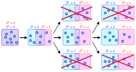
Figure 2: Illustration of quasi-static decomposition described by the family of potentials (43). A sequence of particle configurations. $N=8$, $N^{\rm L}=5$, and $N^{\rm R}=3$. The case $\alpha=0$ is on the leftmost side, and the case $\alpha=1$ on the rightmost side. $(R^{\rm L}_{0},R^{\rm R}_{0})=(D,D)$, $(R^{\rm L}_{1},R^{\rm R}_{1})=(D^{\rm L},D^{\rm R})$, and $R^{\rm L}_{\alpha}\cap R^{\rm R}_{\alpha}\not=\phi,D$ for $0<\alpha<1$. ${\hat{N}}^{\rm L}$ and ${\hat{N}}^{\rm R}$ denotes the number of particles in the region $R^{\rm L}_{\alpha}$ and $R^{\rm R}_{\alpha}$, respectively. Note that ${\hat{N}}^{\rm L}\geq N^{\rm L}$ and ${\hat{N}}^{\rm R}\geq N^{\rm R}$ hold if and only if $V_{\rm con}(\Gamma;{\cal C}_{\alpha})=0$.

Furthermore, we construct a quasi-static process from the parameter set ${\cal C}_{0}$ to ${\cal C}_{1}$. Let $R^{\rm L}_{\alpha}$ and $R^{\rm R}_{\alpha}$ ($0\leq\alpha\leq 1$) be a continuous family of regions satisfying $(R^{\rm L}_{0},R^{\rm R}_{0})=(D,D)$ and $(R^{\rm L}_{1},R^{\rm R}_{1})=(D^{\rm L},D^{\rm R})$. We then define

$$V_{\rm con}(\Gamma;{\cal C}_{\alpha})\equiv\min_{\sigma\in P}\left[\sum_{i=1}^{N^{\rm L}}V_{\rm wall}({\bm{r}}_{\sigma(i)};R^{\rm L}_{\alpha})+\sum_{i=N^{\rm L}+1}^{N}V_{\rm wall}({\bm{r}}_{\sigma(i)};R^{\rm R}_{\alpha})\right].$$ (43)

To see properties of the potential, we define ${\hat{N}}^{\rm L}$ and ${\hat{N}}^{\rm R}$ as the number of particles contained in $R^{\rm L}_{\alpha}$ and $R^{\rm R}_{\alpha}$ for a given particle configuration described by $\Gamma$. We then confirm that ${\hat{N}}^{\rm L}\geq N^{\rm L}$ and ${\hat{N}}^{\rm R}\geq N^{\rm R}$ hold if and only if $V_{\rm con}(\Gamma;{\cal C}_{\alpha})=0$. Keeping this in mind, we find that (43) with $\alpha=0$ is equivalent to (13), and thus (43) with $0\leq\alpha\leq 1$ represents the quasi-static decomposition, as illustrated in Fig. 2. We also note that (43) satisfies (35) for any permutation $\sigma$.

Now, we calculate $\lim_{\kappa\to\infty}Z(T,{\cal C}_{1})$. For later convenience, we define the subset $G$ of permutations $P$ as

$$G\equiv\{\sigma\in P|\sigma(1)<\sigma(2)\cdots<\sigma(N^{\rm L});\sigma(N^{\rm L}+1)<\sigma(N^{\rm L}+2)\cdots<\sigma(N)\}.$$ (44)

For a given phase-space coordinate $\Gamma$ satisfying $V_{\rm con}(\Gamma;{\cal C}_{1})=0$, there is a unique $\sigma\in G$ such that ${\bm{r}}_{\sigma(i)}\in D^{\rm L}$ for $1\leq i\leq N^{\rm L}$ and ${\bm{r}}_{\sigma(i)}\in D^{\rm R}$ for $N^{\rm L}+1\leq i\leq N$. We express this $\sigma$ as $\sigma_{\Gamma}$ to see the $\Gamma$ dependence explicitly. We then have

$$\lim_{\kappa\to\infty}Z(T,{\cal C}_{1})=\int d\Gamma\exp(-\beta H_{0}(\Gamma))\prod_{i=1}^{N^{\rm L}}\chi({\bm{r}}_{\sigma_{\Gamma}(i)}\in D^{\rm L})\prod_{i=N^{\rm L}+1}^{N}\chi({\bm{r}}_{\sigma_{\Gamma}(i)}\in D^{\rm R}).$$ (45)

By substituting $\sum_{\sigma\in G}\delta(\sigma,\sigma_{\Gamma})=1$ into the right-hand side of (45), we rewrite it as

$$\sum_{\sigma\in G}\int d\Gamma\exp(-\beta H_{0}(\Gamma))\prod_{i=1}^{N^{\rm L}}\chi({\bm{r}}_{\sigma(i)}\in D^{\rm L})\prod_{i=N^{\rm L}+1}^{N}\chi({\bm{r}}_{\sigma(i)}\in D^{\rm R}).$$ (46)

Here, using the symmetry property $H_{0}(\Gamma)=H_{0}(\Gamma_{\sigma})$ for any $\sigma\in P$, (46) is further expressed as

$$|G|Z(T,V^{\rm L},N^{\rm L})Z(T,V^{\rm R},N^{\rm R}).$$ (47)

Because

$$|G|=\frac{N!}{N^{\rm L}!N^{\rm R}!},$$ (48)

we obtain (39).

4 Free energy of binary mixtures

In this section, we study a system consisting of two different types of particles, A and B, confined in the cuboid region $D$. Let $\Gamma=(\Gamma^{A},\Gamma^{B})$ be a phase-space coordinate of the system, where

$$\Gamma^{A} =({\bm{r}}^{A}_{1},{\bm{r}}^{A}_{2},\cdots,{\bm{r}}^{A}_{N^{A}},{\bm{p}}^{A}_{1},{\bm{p}}^{A}_{2},\cdots,{\bm{p}}^{A}_{N^{A}}),$$ (49)

$$\Gamma^{B} =({\bm{r}}^{B}_{1},{\bm{r}}^{B}_{2},\cdots,{\bm{r}}^{B}_{N^{B}},{\bm{p}}^{B}_{1},{\bm{p}}^{B}_{2},\cdots,{\bm{p}}^{B}_{N^{B}}).$$ (50)

The Hamiltonian of the system is expressed as

$$H_{0}(\Gamma)=H^{A}(\Gamma^{A})+H^{B}(\Gamma^{B})+H^{AB}(\Gamma)$$ (51)

with

$$H^{A}(\Gamma^{A}) =\sum_{i=1}^{N^{A}}\frac{|{\bm{p}}_{i}|^{2}}{2m^{A}}+\sum_{i<j}V_{\rm int}^{A}(|{\bm{r}}_{i}^{A}-{\bm{r}}_{j}^{A}|),$$ (52)

$$H^{B}(\Gamma^{B}) =\sum_{i=1}^{N^{B}}\frac{|{\bm{p}}_{i}|^{2}}{2m^{B}}+\sum_{i<j}V_{\rm int}^{B}(|{\bm{r}}_{i}^{B}-{\bm{r}}_{j}^{B}|),$$ (53)

$$H^{AB}(\Gamma) =\frac{1}{2}\sum_{i=1}^{N^{A}}\sum_{j=1}^{N^{B}}V_{\rm int}^{AB}(|{\bm{r}}_{i}^{A}-{\bm{r}}_{j}^{B}|).$$ (54)

Here, $V_{\rm int}^{A/B}$ represents a short-range interaction between two particles with the same type $A$ or $B$, and $V_{\rm int}^{\rm AB}$ a short-range interaction between a particle of type $A$ and a particle of type $B$. The system configuration that all the particles are confined in the region $D$ is given by a confining potential

$$V_{\rm con}(\Gamma;{\cal C}_{0})=\sum_{i=1}^{N^{A}}V_{\rm wall}({\bm{r}}_{i}^{A};D)+\sum_{i=1}^{N^{B}}V_{\rm wall}({\bm{r}}_{i}^{B};D),$$ (55)

where ${\cal C}_{0}$ denotes this set of the parameters. The total Hamiltonian is denoted by $H(\Gamma;{\cal C}_{0})$, which is equal to $H_{0}(\Gamma)+V_{\rm con}(\Gamma;{\cal C}_{0})$. We then define the partition function $Z(T,V,N^{A},N^{B})$ by

$$Z(T,V,N^{A},N^{B})=\lim_{\kappa\to\infty}\int d\Gamma\exp(-\beta H(\Gamma;{\cal C}_{0})).$$ (56)

By a similar argument for the derivation of (5), we find that the free energy $F(T,V,N^{A},N^{B})$ of the binary mixture satisfies

$$F(T,V,N^{A},N^{B})=-k_{\rm B}T[\log Z(T,V,N^{A},N^{B})-\bar{\phi}^{(2)}(N^{A},N^{B})]$$ (57)

with a function $\bar{\phi}^{(2)}(N^{A},N^{B})$.

In order to determine $\bar{\phi}^{(2)}(N^{A},N^{B})$, we consider a system configuration that particles of type $A$ are in $D^{\rm L}$, while particles of type $B$ are in $D^{\rm R}$, where $D^{\rm L}$ and $D^{\rm R}$ are separated by greater than the interaction length of particles. This configuration is described by a confining potential

$$V_{\rm con}(\Gamma;{\cal C}_{1})=\sum_{i=1}^{N^{A}}V_{\rm wall}({\bm{r}}_{i}^{A};D^{\rm L})+\sum_{i=1}^{N^{B}}V_{\rm wall}({\bm{r}}_{i}^{B};D^{\rm R}),$$ (58)

Now, using $R^{\rm L}_{\alpha}$ and $R^{\rm R}_{\alpha}$ in the previous section, we can construct a quasi-static process parameterized by ${\cal C}_{\alpha}$ as

$$V_{\rm con}(\Gamma;{\cal C}_{\alpha})=\sum_{i=1}^{N^{A}}V_{\rm wall}({\bm{r}}_{i}^{A};R^{\rm L}_{\alpha})+\sum_{i=1}^{N^{B}}V_{\rm wall}({\bm{r}}_{i}^{B};R^{\rm R}_{\alpha}),$$ (59)

which enforces all particles of type A (and B) to be confined in $R^{\rm L}_{\alpha}$ (and $R^{\rm R}_{\alpha}$). This potential corresponds to a semi-permeable wall for any type of particles. Note that (59) is a standard one-body potential which is different from (43). The relation (3) for the quasi-static process $({\cal C}_{\alpha})_{\alpha=0}^{1}$ is written as

$$F(T,V_{1},N^{A},0)+F(T,V_{2},0,N^{B})-F(T,V,N^{A},N^{B})$$

$$=-k_{\rm B}T[\log Z(T,V_{1},N^{A},0)+\log Z(T,V_{1},0,N^{B})-\log Z(T,V,N^{A},N^{B})].$$ (60)

Here, from the result of the previous section, we have

$$F(T,V_{1},N^{A},0) =-k_{\rm B}T[\log Z(T,V_{1},N^{A},0)-\log N_{A}!-c_{A}N^{A}],$$ (61)

$$F(T,V_{2},0,N^{B}) =-k_{\rm B}T[\log Z(T,V_{2},0,N^{B})-\log N_{B}!-c_{B}N^{B}],$$ (62)

where $c_{A}$ and $c_{B}$ are arbitrary constants. By substituting (57), (61), and (62) into (60), we obtain

$$\bar{\phi}^{(2)}(N^{A},N^{B})=\log N^{A}!+\log N^{B}!+c_{A}N^{A}+c_{B}N^{B}.$$ (63)

Therefore, (57) with (63) becomes

$$F(T,V,N^{A},N^{B})=-k_{\rm B}T\left[\log\frac{Z(T,V,N^{A},N^{B})}{N^{A}!N^{B}!}-c_{A}N^{A}-c_{B}N^{B}\right].$$ (64)

The difference of (64) from (7) comes from the symmetry of the Hamiltonian for permutations. The assumption of the argument is that if the Hamiltonian is not invariant for the exchange of two particle indices, the two particles can be distinguished by the operation of a confining potential.

The above argument implies that the free energy of binary mixtures can be calculated from works measured in numerical simulations or experiments. However, from a practical viewpoint, using the potential (42) may be impossible in experiments and is not efficient in numerical simulations. As shown in Ref. Yoshida , the quasi-static decomposition can be replaced by the measurement-and-feedback with information thermodynamics. Furthermore, the expressions using other quasi-static works can be replaced by the Jarzynski relation Jarzynski , which turns out to be computationally efficient Yoshida .

5 Concluding remarks

We have derived (7) based on a quasi-static decomposition using the potential (42). Our argument stands on the view that free energy is defined by the measurement of thermodynamic quantities, that is, whether or not $N!$ appears in the formula should be determined by thermodynamic considerations. This understanding was first presented over one hundred years ago Ehrenfest . As explained in Sec. 1, it is established that the Gibbs factorial for macroscopic systems is characterized by quasi-static works. The achievement in the present paper is that this known result can be extended to small thermodynamic systems by distinguishing $\log N!$ and $N\log N$. In closing, we briefly discuss other approaches to understand the Gibbs factorial.

In Refs. Warren ; Frenkel , the partition function of a composite system of sub-systems with $(T,V^{\rm L},N^{\rm L})$ and $(T,V^{\rm R},N^{\rm R})$ is given as

$$Z_{\rm comp}(T,V^{\rm L},N^{\rm L},V^{\rm R},N^{\rm R})=\frac{N!}{N^{\rm L}!N^{\rm R}!}Z(T,V^{\rm L},N^{\rm L})Z(T,V^{\rm R},N^{\rm R}).$$ (65)

See Eq. (2) in Warren and Eq. (6) in Frenkel . Although this takes the same form as (39), the left-hand side of (65) is not explicitly defined in Ref. Warren . The Hamiltonian of the composite system should involve a confining potential that is symmetric with respect to permutations of particle indexes. As shown in our paper, we require a special potential (42), but such an example is not illustrated in Ref. Warren . Concerning the last point, in Ref. Frenkel , the composite system is prepared by making a small opening in the separating wall of the two sub-systems with the condition $N^{\rm L}/N^{\rm R}=V^{\rm L}/V^{\rm R}$. However, in this case, $N^{\rm L}$ fluctuates, and thus $N^{\rm L}$ is not a fixed parameter. Nevertheless, (65) may be justified when the thermodynamic limit is taken, because $N^{\rm L}/N$ takes the most probable value. Note that this argument cannot be applied to small thermodynamic systems.

As a slightly different approach, in Ref. Swedsen , the thermodynamic function is defined by the probability of unconstrained thermodynamic variables. For example, in isolated systems, the probability is expressed in terms of thermodynamic entropy Callen ; Einstein . For non-interacting particles in contact with a heat bath, the probability of the number of particles $N^{\rm L}$ in a given region $D^{\rm L}$ of the system is expressed as

$$P(N^{\rm L};T,V,N)=\frac{1}{\tilde{Z}(T,V,N)}\exp(-\beta[F(T,V^{\rm L},N^{\rm L})+F(T,V-V^{\rm L},N-N^{\rm L})]),$$ (66)

where $\tilde{Z}$ is the normalization constant independent of $N^{\rm L}$. Now, one may adopt (66) as a prerequisite for determining the free energy. Because $P(N^{\rm L};T,V,N)$ is calculated from the canonical distribution, we find that (7) holds. The argument is easily generalized to $N$-interacting identical particles for macroscopic systems, which is the standard large deviation theory of thermodynamic systems LD . Nevertheless, this approach cannot be used for small thermodynamic systems except for non-interacting particles.

As a generalization of (3), the Jarzynski relation can be used to determine the free energy from non-equilibrium works Jarzynski . Then, when a non-equilibrium process without the corresponding time-reversed path is considered, the relation takes a modified form MFU . In Ref. Murashita , the free energy is argued using this modified Jarzynski relation with absolute irreversibility. Although the formal result of Eq. (6) in Ref. Murashita is correct, the argument leading to the main result is limited to non-interacting particles. To prove their result for general cases, it is necessary to employ the quasi-static decomposition introduced in the present paper. We thus believe that the essence of the Gibbs factorial is in the quasi-static decomposition, not in the absolute irreversibility.

Finally, we consider quantum systems. Let $\hat{H}({\cal C})$ be a Hamiltonian for $N$-interacting identical particles in a system configuration described by ${\cal C}$. We define the partition function $Z_{\rm QM}({\cal C})$ as

$$Z_{\rm QM}(T,{\cal C})={\rm Tr}(\exp(-\beta\hat{H}({\cal C})).$$ (67)

By repeating a similar argument in Sec. 3, we obtain

$$\lim_{\kappa\to\infty}Z_{\rm QM}(T,{\cal C}_{1})=Z_{\rm QM}(T,V^{\rm L},N^{\rm L})Z_{\rm QM}(T,V^{\rm R},N^{\rm R})$$ (68)

instead of (39). This result leads to

$$F(T,V,N)=-k_{\rm B}T\left[\log{Z_{\rm QM}(T,V,N)}-c_{0}N\right],$$ (69)

instead of (7). The free energy $F$ defined by (8) is equivalent to (69) with $c_{0}=0$. In our viewpoint, (8) should not be a starting point, but interpreted as the result from the prerequisites of free energy. Then, the free energy for both classical and quantum systems can be uniquely determined from the quasi-static works without any confusion, up to an additive constant proportional to $N$. The difference between (7) and (69) comes from the difference in distinguishability of microscopic states for $N$-identical particles. Although this is correct, the distinguishability of microscopic states plays no role in the argument determining the free energy. Rather, the most important issue here is whether or not particles are distinguished by operation of a confining potential.

References

• (1) K. Sekimoto, Stochastic Energetics, Lect. Notes Phys. 799. Springer-Verlag, Berlin (2010).
• (2) U. Seifert, Stochastic thermodynamics, fluctuation theorems and molecular machines, Rep. Prog. Phys. 75, 126001 (2012).
• (3) L. Peliti and S. Pigolotti, Stochastic thermodynamics: an Introduction, Princeton University Press, Princeton (2021).
• (4) N. G. van Kampen, The Gibbs Paradox, edited by W.E. Parry (Pergamon press, Oxford, 1984).
• (5) E. T. Jaynes, in Maximum Entropy and Bayesian Methods, edited by C. R. Smith, G.J. Erickson, and P.O. Neudorfer, (Kluwer Academic, Holland, 1992).
• (6) P. B. Warren, Combinatorial entropy and the statistical mechanics of polydispersity, Phys. Rev. Lett. 80, 1369-1372 (1998).
• (7) R. H. Swendsen, Statistical mechanics of colloids and Boltzmann’s definition of the entropy, American Journal of Physics 74, 187 (2006).
• (8) D. Frenkel, Why colloidal systems can be described by statistical mechanics: Some not very original comments on the Gibbs paradox, Mol. Phys. 112, 2325 (2014).
• (9) Y. Murashita and M. Ueda, Gibbs Paradox Revisited from the Fluctuation Theorem with Absolute Irreversibility, Phys. Rev. Lett. 118, 060601 (2017).
• (10) A. Yoshida and N. Nakagawa, Work relation for determining the mixing free energy of small-scale mixtures, arXiv:2111.06110, to appear in Phys. Rev. Research
• (11) J. M. Horowitz and J. M. R. Parrondo, Designing optimal discrete-feedback thermodynamic engines, New Journal of Physics 13, 123019 (2011).
• (12) C. Jarzynski, Nonequilibrium equality for free energy differences, Phys. Rev. Lett. 78, 2690-2693 (1997).
• (13) P. Ehrenfest and V. Trkal, Ann. Physik 65, 609 (1921).
• (14) H. B. Callen, Thermodynamics and an Introduction to Thermostatistics, 2nd ed. (Wiley, New York, 1985).
• (15) A. Einstein, The theory of the opalescence of homogeneous fluids and liquid mixtures near the critical state, Ann. Phys. 33, 1275 (1910).
• (16) H. Touchette, The large deviation approach to statistical mechanics, Physics Reports, 478, 1-69 (2009).
• (17) Y. Murashita, K. Funo, and M. Ueda, Nonequilibrium equalities in absolutely irreversible processes, Phys. Rev. E 90, 042110 (2014).