Quadrupole topological insulators in Ta${}_{2}M_{3}$Te₅ ($M=$ Ni, Pd) monolayers

Abstract

Higher-order topological insulators have been introduced in the precursory Benalcazar-Bernevig-Hughes quadrupole model, but no electronic compound has been proposed to be a quadrupole topological insulator (QTI) yet. In this work, we predict that Ta${}_{2}M_{3}$Te₅ ($M=$ Pd, Ni) monolayers can be 2D QTIs with second-order topology due to the double-band inversion. A time-reversal-invariant system with two mirror reflections (M_x and M_y) can be classified by Stiefel-Whitney numbers ($w_{1},w_{2}$) due to the combined symmetry $TC_{2z}$. Using the Wilson loop method, we compute $w_{1}=0$ and $w_{2}=1$ for Ta₂Ni₃Te₅, indicating a QTI with $q^{xy}=e/2$. Thus, gapped edge states and localized corner states are obtained. By analyzing atomic band representations, we demonstrate that its unconventional nature with an essential band representation at an empty site, i.e., $A_{g}@4e$, is due to the remarkable double-band inversion on Y-$\Gamma$. Then, we construct an eight-band quadrupole model with $M_{x}$ and $M_{y}$ successfully for electronic materials. These transition-metal compounds of $A_{2}M_{1,3}X_{5}$ ($A$ = Ta, Nb; $M$ = Pd, Ni; $X$ = Se, Te) family provide a good platform for realizing the QTI and exploring the interplay between topology and interactions.

Introduction.

In higher-order topological insulators, the ingap states can be found in ($d-n$)-dimensional edges ($n>1$), such as the corner states of two-dimensional (2D) systems or the hinge states of three-dimensional systems Benalcazar et al. (2017); Schindler et al. (2018a); Song et al. (2017); Langbehn et al. (2017); Schindler et al. (2018b); Ezawa (2018); Khalaf (2018); Wang et al. (2019); Benalcazar et al. (2019a); Yue et al. (2019); Xu et al. (2019); Wieder et al. (2020). Different from topological insulators with ($d-1$)-dimensional edge states, the Chern numbers or $\mathbb{Z}_{2}$ numbers in higher-order topological insulators are zero. The higher-order topology can be captured by topological quantum chemistry Bradlyn et al. (2017); Elcoro et al. (2021); Gao et al. (2022a); Nie et al. (2021a, b); Gao et al. (2022b), nested Wilson loop method Benalcazar et al. (2017); Wang et al. (2019) and second Stiefel-Whitney (SW) class Fang et al. (2015); Zhao et al. (2016); Zhao and Lu (2017); Ahn et al. (2019a, b); Wu et al. (2019); Pan et al. (2022). Using topological quantum chemistry Bradlyn et al. (2017), the higher-order topological insulator can be diagnosed by the decomposition of atomic band representations (aBRs) as an unconventional insulator (or obstructed atomic insulator) with mismatching of electronic charge centers and atomic positions Nie et al. (2021a, b); Xu et al. (2021); Gao et al. (2022b). In contrast to dipoles (Berry phase) for topological insulators, the higher-order topological insulators can be understood by multipole moments Benalcazar et al. (2017). In a 2D system, the second-order topology corresponds to the quadrupole moment, which can be diagnosed by the nested Wilson loop method Benalcazar et al. (2017); Wang et al. (2019); Ahn et al. (2019b). When the system contains space-time inversion symmetries, such as $PT$ and $C_{2z}T$, where the $P$ and $T$ represent inversion and time-reversal symmetries, the second-order topology can be described by the second SW number ($w_{2}$) Wieder and Bernevig (2018); Ahn et al. (2019b). The second SW number $w_{2}$ is a well-defined 2D topological invariant of an insulator only when the first SW number $w_{1}=0$. Usually, a 2D quadrupole topological insulator (QTI) with $w_{1}=0,w_{2}=1$ has gapped edge states and degenerate localized corner states, which are pinned at zero energy (being topological) in the presence of chiral symmetry. When the degenerate corner states are in the energy gap of bulk and edge states, the fractional corner charge can be maintained due to filling anomaly Benalcazar et al. (2019b).

So far, various 2D systems are proposed to be SW insulators with second-order topology, such as monolayer graphdiyne Sheng et al. (2019); Lee et al. (2020), liganded Xenes Qian et al. (2021); Pan et al. (2022), $\beta$-Sb monolayer Gao et al. (2022b) and Bi/EuO Chen et al. (2020). However, no compound has been proposed to be a QTI with M_x and M_y symmetries. After considering many-body interactions in transition-metal compounds, superconductivity, exciton condensation and Luttinger liquid could emerge in a transition-metal QTI. In recent years, van der Waals layered materials of $A_{2}M_{1,3}X_{5}$ ($A$ = Ta, Nb; $M$ = Pd, Ni; $X$ = Se, Te) family have attracted attentions because of their special properties, such as quantum spin Hall effect in Ta₂Pd₃Te₅ monolayer Guo et al. (2021); Wang et al. (2021), excitons in Ta₂NiSe₅ Wakisaka et al. (2009); Lu et al. (2017); Mazza et al. (2020), and superconductivity in Nb₂Pd₃Te₅ and doped Ta₂Pd₃Te₅ Higashihara et al. (2021). In particular, the monolayers of $A_{2}M_{1,3}X_{5}$ family can be exfoliated easily, serving as a good platform for studying topology and interactions in lower dimensions.

In this work, we predict that based on first-principles calculations, Ta₂Ni₃Te₅ monolayer is a 2D QTI. Using the Wilson-loop method, we show that its SW numbers are $w_{1}=0$ and $w_{2}=1$, corresponding to the second-order topology. We also solve the aBR decomposition for Ta₂Ni₃Te₅ monolayer, and find that it is unconventional with an essential band representation (BR) at an empty Wykoff position (WKP), $A_{g}@4c$, which origins from the remarkable double-band inversion on Y–$\Gamma$ line. To verify the QTI phase, we compute the energy spectrum of Ta₂Ni₃Te₅ monolayer with open boundary conditions in both $x$ and $y$ directions and obtain four degenerate corner states. Then, we construct an eight-band quadrupole model with $M_{x}$ and $M_{y}$ successfully. The double-band-inversion picture widely happens in the band structures of $A_{2}M_{1,3}X_{5}$ family. The Ta${}_{2}M_{3}$Te₅ monolayers are 2D QTI candidates for experimental realization in electronic systems.

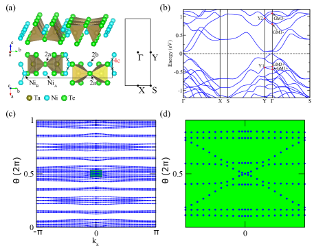
Figure 1: (a) The crystal structure, Wyckoff positions and Brillouin zone (BZ) of Ta₂Ni₃Te₅ monolayer. (b) Band structure and irreps at Y and $\Gamma$ of Ta₂Ni₃Te₅ monolayer. (c) The 1D $k_{y}$-direct Wilson bands as a function of $k_{x}$ calculated in the DFT code. (d) Close-up of the green region in (c), with one crossing of Wilson bands at $\theta=\pi$ indicating the second SW class $w_{2}=1$.

Band structures.

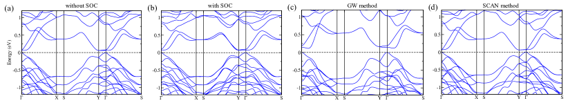
Figure S2: The comparisons of band structures of Ta₂Ni₃Te₅ monolayers (a) without SOC, (b) with SOC, (c) using GW method, (d) using SCAN method. The band gaps and double band inversions are remained in these band structures using different methods.

The band structure of Ta₂Ni₃Te₅ monolayer suggests that it is an insulator with a band gap of 65 meV. We have checked that spin-orbit coupling (SOC) has little effect on the band structure (Fig. S2(b)). We also checked the band structures using GW method and SCAN method, and we find that the band gap remains using these methods (the corresponding band structures are shown in Appendix A). As shown in the orbital-resolved band structures of Fig. 3(a-c), although low-energy bands near the Fermi level ($E_{F}$) are mainly contributed by Ta-$d_{z^{2}}$ orbitals (two conduction bands) and Ni_A-$d_{xz}$ orbitals (two valence bands), the inverted bands of $\{\rm{Y}2;\rm{GM}1-,\rm{GM}3-\}$ come from Te-$p_{x}$ orbitals. The irreducible representations (irreps) Gao et al. (2021) at Y and $\Gamma$ are denoted for the inverted bands in Fig. 1(b). We notice that the double-band inversion between $\{\rm{Y}2;\rm{GM}1-,\rm{GM}3-\}$ bands and $\{\rm{Y}1;\rm{GM}1+,\rm{GM}3+\}$ bands is remarkable, about 1 eV.

Atomic band representations.

To analyze the band topology, the decomposition of aBR is performed. In a unit cell of Ta₂Ni₃Te₅ monolayer in Fig. 1(a), four Ta atoms, four Ni_B atoms and eight Te atoms are located at different $4e$ WKPs. The rest two Te atoms and two Ni_A atoms are located at $2a$ and $2b$ WKPs respectively. The aBRs are obtained from the crystal structure by pos2aBR Nie et al. (2021a, b); Gao et al. (2022b), and irreps of occupied states are calculated by IRVSP Gao et al. (2021) at high-symmetry $k$-points. Then, the aBR decomposition is solved online -- http://tm.iphy.ac.cn/UnconvMat.html. The results are listed in Table S2 of Appendix B. Instead of being a sum of aBRs, we find that the aBR decomposition of the occupied bands has to include an essential BR at an empty WKP, i.e., $A_{g}@4c$. As illustrated in Fig. 1(a), the charge centers of the essential BR are located at the middle of Ni_B-Ni_B bonds (i.e., the $4c$ WKP), indicating that the Ta₂Ni₃Te₅ monolayer is a 2D unconventional insulator with second-order topology.

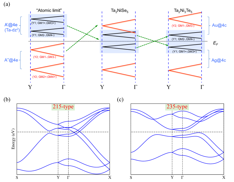
Figure 2: (a) The diagram of double-band inversion along Y--$\Gamma$ line. The schematic band structures of (b) 215-type semimetal and (c) 235-type insulator. The double-band inversion happens in both cases. The crossing points on the $\Gamma$--X line are part of the nodal line.

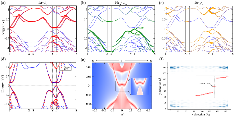
Figure 3: The orbital-resolved band structures of (a) $d_{z^{2}}$ orbitals of Ta atoms, (b) $d_{xz}$ orbitals of Ni_A atoms, and (c) $p_{x}$ orbitals of Te atoms. (d) The comparison between band structures of maximally localized Wannier functions and DFT results. (e) (01)-edge states around $\Gamma$. (f) The charge distribution of four corner states. The insert shows the energy spectrum of the tight-binding model with open boundaries in $x$ and $y$ directions.

Double-band inversion.

In an ideal atomic limit, Te-$p$ orbitals and Ni-$d$ orbitals are occupied, while Ta-$d$ orbitals are fully unoccupied. Thus, all the occupied bands are supposed to be the aBRs of Te-$p$ and Ni-$d$ orbitals, as shown in the left panel of Fig. 2(a). However, in the monolayers of $A_{2}M_{1,3}X_{5}$ family (see their band structures in Appendix A), a double-band inversion happens between the occupied aBR $A^{\prime\prime}@4e$ (Te-$p_{x}$ and Ni-$d$) and unoccupied aBR $A^{\prime}@4e$ (Ta-$d_{z^{2}}$), as shown in the right two panels of Fig. 2(a). When the double-band inversion happens between $\{\rm{Y}2;\rm{GM}1-,\rm{GM}3-\}$ and $\{\rm{Y}1;\rm{GM}2-,\rm{GM}4-\}$ on Y--$\Gamma$ line, it results in a semimetal for Ta₂NiSe₅ monolayer (215-type; Fig. 2(b)). When it happens between $\{\rm{Y}2;\rm{GM}1-,\rm{GM}3-\}$ and $\{\rm{Y}1;\rm{GM}1+,\rm{GM}3+\}$ in Fig. 2(c), the system becomes a 2D QTI for Ta₂Ni₃Te₅ monolayer (235-type), resulting in the essential BR of $A_{g}@4c$.

Second Stiefel-Whitney class $w_{2}=1$.

To identify the second-order topology of the monolayers, we compute the second SW number by the Wilson-loop method. The first SW class ($w_{1}$) is,

$$\evaluated{w_{1}}_{C}=\frac{1}{\pi}\oint_{C}\differential{{\bf\it k}}\cdot\Tr{\bf\it\mathcal{A}}({\bf\it k})$$ (1)

where ${\bf\it\mathcal{A}}_{mn}({\bf\it k})=\matrixelement{u_{m}({\bf\it k})}{{\text{i}}\gradient_{{\bf\it k}}}{u_{n}({\bf\it k})}$ Ahn et al. (2019a). The second SW class ($w_{2}$) can be computed by the nested Wilson-loop method, or simply by $m$ module 2, where $m$ is the number of crossings of Wilson bands at $\theta=\pi$. It should be noted that $w_{2}$ is well-defined only when $w_{1}=0$. With $w_{1}=0$, $w_{2}$ can be unchanged when choosing the unit cell shifting a half lattice constant. The 1D Wilson-loops are computed along $k_{y}$. The computed phases of the eigenvalues of Wilson-loop matrices $W_{y}(k_{x})$ (Wilson bands) are shown in Fig. 1(c) as a function of $k_{x}$. The results show that the first SW class is $w_{1}=0$. In addition, there is one crossing of Wilson bands at $\theta=\pi$ [Fig. 1(d)], indicating the second SW class $w_{2}=1$. The quadruple moment $q^{xy}=e/2$ calculated by the nested Wilson-loop method in Appendix C. Therefore, the Ta₂Ni₃Te₅ monolayer is a QTI with a nontrivial second SW number.

Edge spectrum and corner states.

From the orbital-resolved band structures (Fig. 3), the maximally localized Wannier functions of Ta-$d_{z^{2}}$, Ni_A-$d_{xz}$ and Te-$p_{x}$ orbitals are extracted, to construct a 2D tight-binding (TB) model of Ta₂Ni₃Te₅ monolayer. As shown in Fig. 3(d), the obtained TB model fits the density functional theory (DFT) band structure well. First, we compute the (01)-edge spectrum with open boundary condition along $y$. Instead of gapless edge states for a 2D $\mathbb{Z}_{2}$-nontrivial insulator, gapped edge states are obtained for the 2D QTI [Fig. 3(e)]. Then, we explore corner states as the hallmark of the 2D QTI. We compute the energy spectrum for a nanodisk. For concreteness, we take a rectangular-shaped nanodisk with $50\times 10$ unit cells, preserving both $M_{x}$ and $M_{y}$ symmetries in the 0D geometry. The obtained discrete spectrum for this nanodisk is plotted in the inset of Fig. 3(f). Remarkably, one observes four degenerate states near $E_{F}$. The spatial distribution of these four-fold modes can be visualized from their charge distribution, as shown in Fig. 3(f). Clearly, they are well localized at the four corners, corresponding to isolated corner states.

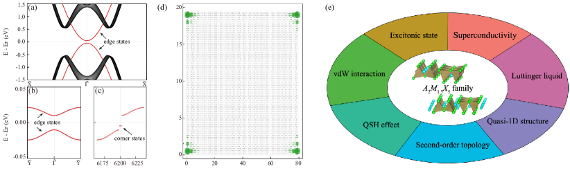
Figure 4: Energy spectrum for (a) the (01)-edge, (b) the (10)-edge, and (c) a $M_{x}$- and $M_{y}$-symmetric disk of $80\times 20$ unit cells of the minimum model with chiral symmetry slightly broken ($\delta=-0.1$). (d) The spatial distribution of four degenerate in-gap states in (c). (e) The diverse properties of $A_{2}M_{1,3}X_{5}$ ($A$ = Ta, Nb; $M$ = Pd, Ni; $X$ = Se, Te) family.

Minimum model for the 2D QTI.

As shown in Fig. 2, the minimum model for the 2D QTI should be consisted of two BRs of $A^{\prime}@4e$ and $A^{\prime\prime}@4e$. Based on the situation of Ta₂Ni₃Te₅ monolayer in Fig. 2(c), the minimum effective model is derived as below,

$$H_{\rm TB}({\bf\it k})=\begin{pmatrix}H_{\rm Ta}({\bf\it k})&H_{\rm hyb}({\bf\it k})\\ {H_{\rm hyb}({\bf\it k})}^{\scriptstyle{\dagger}}&H_{\rm Ni}({\bf\it k})\end{pmatrix}$$ (2)

The terms of $H_{\rm Ta}({\bf\it k}),H_{\rm Ni}({\bf\it k})$ and $H_{\rm int}({\bf\it k})$ are $4\times 4$ matrices, which read

$$H_{\rm Ta}({\bf\it k})= \;\bqty{\varepsilon_{s}+2t_{s1}\cos(k_{x})}\sigma_{0}\tau_{0}+t_{s2}\gamma_{1}({\bf\it k})+t_{s3}\sigma_{0}\tau_{x},$$ (3)

$$H_{\rm Ni}({\bf\it k})= \;\bqty{\varepsilon_{p}+2t_{p1}\cos(k_{x})}\sigma_{0}\tau_{0}+t_{p2}\gamma_{2}({\bf\it k})+t_{p3}\sigma_{0}\tau_{x},$$

$$H_{\rm hyb}({\bf\it k})= \;2{\text{i}}t_{sp}\sin(k_{x})\gamma_{3}({\bf\it k}).$$

The $\gamma_{1,2,3}({\bf\it k})$ matrices are given explicitly in Appendix D.

Table 1: Parameters of the TB model for the QTI with chiral symmetry when $\delta=0$.

$\varepsilon_{s}$	$t_{s1}$	$t_{s2}$	$t_{s3}$	$t_{sp}$	$\varepsilon_{p}$	$t_{p1}$	$t_{p2}$	$t_{p3}$
2.05	-1	-0.8	-0.2	0.3	-2.05	1	0.8	0.2(1+$\delta$)

We find that $t_{s1}<0$ and $t_{p1},t_{p2}>0$ for the $A_{2}M_{1,3}X_{5}$ family ($t_{s3}$ and $t_{p3}$ are small). When $\varepsilon_{s}+2t_{s1}-2\absolutevalue{t_{s2}}<\varepsilon_{p}+2t_{p1}+2t_{p2}$, the double-band inversion happens in the monolayers of this family. By fitting the DFT bands, we obtain $t_{s2}>0$ for the 215-type, while $t_{s2}<0$ for the 235-type. When $\varepsilon_{p}=-\varepsilon_{s}$ and $t_{pi}=-t_{si}(i=1,2,3)$, the model is chiral symmetric (i.e., $\delta=0$ in Table 1). Since the second SW insulator or QTI is topological in the presence of chiral symmetry, we would focus on the model (almost respecting chiral symmetry) in the following discussion.

Analytic solution of (01)-edge states

As the remnants of the QTI phase, the localized edge states can be solved analytically for the minimum model. For the (01)-edge, one can treat the model $H_{\rm TB}({\bf\it k})$ as two parts, $H_{0}({\bf\it k})$ and $H^{\prime}({\bf\it k})$,

$$H_{0}({\bf\it k})= \;\begin{pmatrix}t_{s2}\gamma_{1}({\bf\it k})+t_{s3}\sigma_{0}\tau_{x}&0\\ 0&t_{p2}\gamma_{2}({\bf\it k})+t_{p3}\sigma_{0}\tau_{x}\end{pmatrix}$$ (4)

$$H^{\prime}({\bf\it k})= \;\begin{pmatrix}\bqty{\varepsilon_{s}+2t_{s1}\cos(k_{x})}\sigma_{0}\tau_{0}&H_{\rm hyb}({\bf\it k})\\ {H_{\rm hyb}({\bf\it k})}^{\scriptstyle{\dagger}}&\bqty{\varepsilon_{p}+2t_{p1}\cos(k_{x})}\sigma_{0}\tau_{0}\end{pmatrix}$$

Note that there is a pair of Dirac points $(\pm k_{x}^{D},0)$, with $k_{x}^{D}=\arccos\left[\frac{1}{2}\pqty{\frac{t_{s3}}{t_{s2}}}^{2}-1\right]$. Since $k_{x}$ is still a good quantum number on the (01)-edge, expanding $k_{y}$ to the second order, the zero-mode equation $H_{0}(k_{x},-{\text{i}}\partial_{y})\Psi(k_{x},y)=0$ can be solved for $y\in[0,+\infty)$. Taking the trial solution of $\Psi(k_{x},y)=\psi(k_{x})e^{\lambda y}$, we obtain the secular equation and the solution of $\lambda=\pm\lambda_{\pm}$, where

$$\lambda_{\pm}=1\pm\sqrt{\frac{t_{s3}^{2}}{(1+\cos(k_{x}))t_{s2}^{2}}-1}$$ (5)

With the boundary conditions $\Psi(k_{x},0)=\Psi(k_{x},+\infty)=0$, only $-\lambda_{\pm}$ are permitted.

In the $k_{x}$ regime of $\left[-{\bf\it k}_{x}^{D},{\bf\it k}_{x}^{D}\right]$, the edge zero-mode states are $\Psi(k_{x},y)=\bqty{C_{1}(k_{x})\phi_{1}(k_{x})+C_{2}(k_{x})\phi_{2}(k_{x})}$ $\pqty{e^{-\lambda_{+}y}-e^{-\lambda_{-}y}}$ with

$$\phi_{1}(k_{x})= \;\begin{pmatrix}-\frac{(1+e^{-{\text{i}}k_{x}})t_{s2}}{t_{s3}}&0&1&0&0&0&0&0\end{pmatrix}^{\rm T}$$ (6)

$$\phi_{2}(k_{x})= \;\begin{pmatrix}0&0&0&0&-\frac{t_{p3}}{(1+e^{{\text{i}}k_{x}})t_{p2}}&0&1&0\end{pmatrix}^{\rm T}$$

The edge zero states are Fermi arcs that linking the pair of projected Dirac points $(\pm k_{x}^{D},0)$. Once $H^{\prime}({\bf\it k})$ included, the effective (01)-edge Hamiltonian is,

$$H^{eff}_{\rm 01} =\bra{\Phi}H({\bf\it k})\ket{\Phi}$$ (7)

$$=\begin{pmatrix}\varepsilon_{s}+2t_{s1}\cos(k_{x})&0\\ 0&\varepsilon_{p}+2t_{p1}\cos(k_{x})\end{pmatrix}$$

where $\ket{\Phi}\equiv\ket{\phi_{1}(k_{x}),\phi_{2}(k_{x})}$. Two edge spectra are obtained in Fig. 4 (a).

Effective SSH model on (10)-edge and corner states

Similarly, we derive the (10)-edge modes as $[F_{1}(k_{y})\varphi_{1}(k_{y})+F_{2}(k_{y})\varphi_{2}(k_{y})]\left(e^{-\Lambda_{+}x}-e^{-\Lambda_{-}x}\right)$ with

$$\varphi_{1}=\begin{pmatrix}0\\ 1-\Delta_{s}\\ 1-\Delta_{s}e^{ik_{y}}\\ 0\\ -1+\Delta_{p}\\ 0\\ 0\\ -1+\Delta_{p}e^{-ik_{y}}\end{pmatrix},\varphi_{2}=\begin{pmatrix}e^{-ik_{y}}\left(1-\Delta_{s}\right)\\ 0\\ 0\\ 1-\Delta_{s}e^{-ik_{y}}\\ 0\\ -1+\Delta_{p}\\ -e^{-ik_{y}}+\Delta_{p}\\ 0\end{pmatrix}.$$ (8)

Here, $\Lambda_{\pm}=\frac{2t_{sp}\pm\sqrt{4t_{sp}^{2}-2(2t_{s1}+t_{s2})(2t_{s1}+2t_{s2}+\varepsilon_{s})}}{2t_{s1}+t_{s2}}$, $\Delta_{s}=\left(\frac{t_{s3}}{2t_{s2}}\right)^{2}$, and $\Delta_{p}=\left(\frac{t_{p3}}{2t_{p2}}\right)^{2}$. Then we obtain the effective Hamiltonian on (10) edge below,

$$H^{eff}_{\rm 10} =\begin{pmatrix}0&v+we^{-ik_{y}}\\ v+we^{ik_{y}}&0\end{pmatrix},$$ (9)

$$w =t_{s3}+t_{p3}-4t_{s3}\Delta_{s},$$

$$v =t_{s3}+t_{p3}-4t_{p3}\Delta_{p}$$

When $\delta=0$, the minimum QTI model is chiral symmetric and it is gapless on the (10) edge (preserving $M_{y}$ symmetry). When the chiral symmetry is slightly broken ($\delta\neq 0$), the $H^{eff}_{10}$ becomes an Su-Schrieffer-Heeger model ($\delta<0$ nontrivial; $\delta>0$ trivial), as presented in Fig. 4(b-d). As a result, we obtain a solution state on the end of the edge mode, i.e., the corner. As long as the energy of the corner state is located in the gap of bulk and edge states, the corner state is well localized at the corners, as shown in Fig. 4(c,d).

Discussion.

In Ta₂NiSe₅ monolayer, the double-band inversion has also happened between Ta-$d_{z2}$ and Te-$p_{x}$ states, about 0.4 eV, resulting in a semimetal with a pair of nodal lines in the 215-type. The highest valence bands on Y--$\Gamma$ are from the inverted Ta-$d_{z^{2}}$ states. However, in Ta₂Ni₃Te₅ monolayer, the double-band inversion strength becomes remarkable, $\sim$ 1 eV, which is ascribed to the filled $B$-type voids and more extended Te-$p$ states. On the other hand, the highest valence bands become Ni_A-$d_{xz}$ states (slightly hybridized with Te-$p_{x}$ states). It is insulating with a small gap of 65 meV. When it comes to $A_{2}$Pd₃Te₅ monolayer, the remarkable inversion strength is similar to that of Ta₂Ni₃Te₅. But the Pd_A-$d_{xz}$ states go upwards further due to more expansion of the $d$-orbitals and the energy gap becomes almost zero in Ta₂Pd₃Te₅. In short, the double-band inversion happens in all these monolayers, while the band gap of the 235-type changes from positive (Ta₂Ni₃Te₅), to nearly zero (Ta₂Pd₃Te₅ with a tiny band overlap), to negative (Nb₂Pd₃Te₅), as shown in Fig. S1. Although the band structure of Ta₂Pd₃Te₅ bulk is metallic without SOC Guo et al. (2021); Wang et al. (2021); Higashihara et al. (2021), the monolayer could become a QSH insulator upon including SOC in Ref.Guo et al. (2021). Since their bulk materials are van der Waals layered compounds, the bulk topology and properties strongly rely on the band structures of the monolayers in the $A_{2}M_{1,3}X_{5}$ family.

As we find in Ref. Guo et al. (2021), the band topology of Ta₂Pd₃Te₅ monolayer is lattice sensitive. By applying $>1$% uniaxial compressive strain along $b$, it becomes a $\mathbb{Z}_{2}$-trivial insulator, being a QTI. On the other hand, due to the quasi-1D crystal structure, the screening effect of carriers is relatively weak and the electron-hole Coulomb interaction may be substantial for exciton condensation. The 1D in-gap edge states as remnants of the QTI are responsible for the observed Luttinger-liquid behavior.

In conclusion, we predict that Ta${}_{2}M_{3}$Te₅ monolayers can be QTIs by solving aBR decomposition and computing SW numbers. Through aBR analysis, we conclude that the second-order topology comes from an essential BR at the empty site ($A_{g}@4c$), and it origins from the remarkable double-band inversion. The double-band inversion also happens in the band structure of Ta₂NiSe₅ monolayer. The second SW number of Ta₂Ni₃Te₅ monolayer is $w_{2}=1$, corresponding to a QTI. Therefore, we obtain edge states and corner states of the monolayer. The eight-band quadrupole model with M_x and M_y has been constructed successfully for electronic materials. With the large double-band inversion and small band energy gap/overlap, these transition-metal materials of $A_{2}M_{1,3}X_{5}$ family provide a good platform to study the interplay between the topology and interactions (Fig. 4(e)).

Method.

Our first-principles calculations were performed within the framework of the DFT using the projector augmented wave method Blochl (1994); Kresse and Joubert (1999), as implemented in Vienna ab-initio simulation package (VASP) Kresse and Furthmuller (1996a, b). The Perdew-Burke-Ernzerhof (PBE) generalized gradient approximation exchange-correlations functional Perdew et al. (1996) was used. SOC is neglected in the calculations except Supplementary Figure 2(b). We also used SCAN Sun et al. (2015) and GW Shishkin and Kresse (2006) method when checking the band gap. In the self-consistent process, 16 $\times$ 4 $\times$ 1 $k$-point sampling grids were used, and the cut-off energy for plane wave expansion was 500 eV. The irreps were obtained by the program IRVSP Gao et al. (2021). The maximally localized Wannier functions were constructed by using the Wannier90 package Pizzi et al. (2020). The edge spectra are calculated using surface Green’s function of semi-infinite system Sancho et al. (1984, 1985).

Appendix

A The band structures of the monolayers of $A_{2}M_{1,3}X_{5}$ family

The space group of relaxed Ta₂Ni₃Te₅ monolayer is $Pmmn$ (No. 59). The symmetry operators are inversion, $\widetilde{C}_{2x}=\{C_{2x}|1/2,0,0\}$, $\widetilde{C}_{2y}=\{C_{2y}|0,1/2,0\}$ and $\widetilde{C}_{2z}=\{C_{2z}|1/2,1/2,0\}$. Although $P$ is weakly broken in the exfoliated monolayer from the bulk, it will be regained after relaxation. The change of the band structure is minute, as presented in Fig. S1(c-d). In a unit cell of Ta₂Ni₃Te₅ monolayer in Fig. 1(a), four Ta atoms, four Ni_B atoms and eight Te atoms are located at $4e$ WKPs. The rest two Te atoms and two Ni_A atoms are differently located at $2a$ and $2b$ WKPs respectively. They form 1D Ta₂Te₅ double chains. Unlike only $A$-type voids filled in Ta₂NiSe₅, both $A$- and $B$-types of tetrahedral voids are filled by Ni_A and Ni_B respectively in Ta₂Ni₃Te₅ Guo et al. (2021) (Fig. 1(a)).

There are two phases of bulk Ta₂NiSe₅, which are $C2/c$ (No. 15, low-temperature phase) and $Cmcm$ (No. 63, high-temperature phase). The exfoliated Ta₂NiSe₅ monolayer of $C2/c$ is insulator after relaxation (Fig. S1(a)). As shown in Fig. S1(b), the exfoliated Ta₂NiSe₅ monolayer of $Cmcm$ is semimetal, and the compatibility relationship is consistent with band inversion process in Fig. 2(a). In addition, the Ta₂NiSe₅ is proposed to be an exciton insulator Mazza et al. (2020). In literature, there is another argument about the band gap opening, which is the single-particle band hybridization after the structural phase transition (form high-temperature SG63 to low-temperature SG 15). The space group of bulk Ta${}_{2}M_{3}$Te₅($M$ = Ni, Pd) is $Pnma$ (No. 62), and space group of the corresponding exfoliated monolayer is $Pmn2_{1}$ (No. 31). However, the relaxed Ta₂Ni₃Te₅ monolayer structure has inversion symmetry, and the corresponding space group becomes $Pmmn$ (No. 59). Thus, the inversion was imposed into Ta${}_{2}M_{3}$Te₅ monolayers with tiny atom positions movements, and the corresponding band structures are also calculated, as shown in Fig. S1(c-h). In addition, with inversion symmetry, the irreps can be distinguished by parity and the aBR decomposition can be done easily.

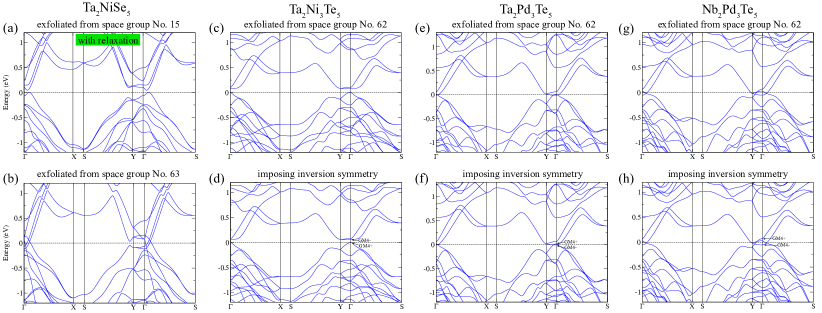
Figure S1: The comparisons of band structures of (a-b) Ta₂NiSe₅, (c-d) Ta₂Ni₃Te₅, (e-f) Ta₂Pd₃Te₅, (g-h) Nb₂Pd₃Te₅ monolayers. The lower panels share the same space group #59. The 235-type band gap ($E_{g}=E_{GM4-}-E_{GM4+}$) changes for 0.068 eV for Ta₂Ni₃Te₅, to -0.023 eV for Ta₂Pd₃Te₅, to -0.124 eV for Nb₂Pd₃Te₅ monolayers.

B The aBR decomposition of Ta₂Ni₃Te₅

As shown in Table. S1, we find that $A^{\prime}@4e+A^{\prime\prime}@4e=Ag@4c+Au@4c$ in aBRs for $Pmmn$ space group. The WKPs, aBRs and the aBR decomposition of Ta₂Ni₃Te₅ monolayer are given in Table. S2.

Table S1: The aBRs for $Pmmn$ space group at $4e$ and $4c$ WKPs, we can find $A^{\prime}@4e+A^{\prime\prime}@4e=Ag@4c+Au@4c$.

	$A^{\prime}@4e$	$A^{\prime\prime}@4e$	$Ag@4c$	$Au@4c$
$\Gamma$	$\Gamma_{1+}\oplus\Gamma_{2-}\oplus\Gamma_{3+}\oplus\Gamma_{4-}$	$\Gamma_{1-}\oplus\Gamma_{2+}\oplus\Gamma_{3-}\oplus\Gamma_{4+}$	$\Gamma_{1+}\oplus\Gamma_{2+}\oplus\Gamma_{3+}\oplus\Gamma_{4+}$	$\Gamma_{1-}\oplus\Gamma_{2-}\oplus\Gamma_{3-}\oplus\Gamma_{4-}$
S	$S_{1}\oplus$$S_{2}$	$S_{1}\oplus$$S_{2}$	$S_{1}\oplus$$S_{2}$	$S_{1}\oplus$$S_{2}$
X	$X_{1}\oplus$$X_{2}$	$X_{1}\oplus$$X_{2}$	$X_{1}\oplus$$X_{2}$	$X_{1}\oplus$$X_{2}$
Y	$2Y_{1}$	$2Y_{2}$	$Y_{1}\oplus$$Y_{2}$	$Y_{1}\oplus$$Y_{2}$

Table S2: The aBRs, BR decomposition for $Pmmn$ Ta₂Ni₃Te₅ monolayer.

Atom	WKP$(q)$	Symm.	Orbital	Irrep$(\rho)$	aBR($\rho@q$)	Occ.
Ta	4$e$	$m$	$d_{x^{2}-y^{2}}$	$A^{\prime}$	$A^{\prime}@$4$e$
			$d_{z^{2}}$	$A^{\prime\prime}$	$A^{\prime}@$4$e$
			$d_{yz}$	$A^{\prime\prime}$	$A^{\prime}@$4$e$
			$d_{xz}$	$A^{\prime\prime}$	$A^{\prime\prime}@$4$e$
			$d_{xy}$	$A^{\prime\prime}$	$A^{\prime\prime}@$4$e$
NiA	2$b$	$mm2$	$d_{z^{2}}$	$A_{1}$	$A_{1}@$2$b$	yes
			$d_{x^{2}-y^{2}}$	$A_{1}$	$A_{1}@$2$b$	yes
			$d_{xy}$	$A_{2}$	$A_{2}@$2$b$	yes
			$d_{xz}$	$B_{1}$	$B_{1}@$2$b$	yes
			$d_{yz}$	$B_{2}$	$B_{2}@$2$b$	yes
NiB	4$e$	$m$	$d_{z^{2}}$	$A^{\prime}$	$A^{\prime}@$4$e$	yes
			$d_{x^{2}-y^{2}}$	$A^{\prime}$	$A^{\prime}@$4$e$	yes
			$d_{yz}$	$A^{\prime}$	$A^{\prime}@$4$e$	yes
			$d_{xz}$	$A^{\prime\prime}$	$A^{\prime\prime}@$4$e$	yes
			$d_{xy}$	$A^{\prime\prime}$	$A^{\prime\prime}@$4$e$	yes
Te1	2$a$	$mm2$	$p_{z}$	$A_{1}$	$A_{1}@$2$a$	yes
			$p_{x}$	$B_{1}$	$B_{1}@$2$a$	yes
			$p_{y}$	$B_{2}$	$B_{2}@$2$a$	yes
Te2	4$e$	$m$	$p_{z}$	$A^{\prime}$	$A^{\prime}@$4$e$	yes
			$p_{y}$	$A^{\prime}$	$A^{\prime}@$4$e$	yes
			$p_{x}$	$A^{\prime\prime}$	$A^{\prime\prime}@$4$e$	yes
Te3	4$e$	$m$	$p_{z}$	$A^{\prime}$	$A^{\prime}@$4$e$	yes
			$p_{y}$	$A^{\prime}$	$A^{\prime}@$4$e$	yes
			$p_{x}$	$A^{\prime\prime}$	$A^{\prime\prime}@$4$e$
					$A_{g}@$4$c$	yes

C Wilson-loop method

The Wilson-loop method is widely applied in identifying topology in bands. A Hamiltonian satisfies,

$$H(k_{x},k_{y})\ket{u_{n}(k_{x},k_{y})}=E_{n}(k_{x},k_{y})\ket{u_{n}(k_{x},k_{y})}$$ (10)

with $n_{\rm occ}$ occupied energy bands. We can define the overlap matrix,

$$M_{y}^{mn}(k_{x};k_{y}^{j},k_{y}^{j+1})=\innerproduct{u_{m}(k_{x},k_{y}^{j})}{u_{n}(k_{x},k_{y}^{j+1})}$$ (11)

where $k_{y}^{j}=2{\pi}j/N$, $m,n=1,2,...,n_{\rm occ}$, and,

$${\mathcal{W}}_{y}(k_{x})=\prod_{j=0}^{N-1}M_{y}(k_{x};k_{y}^{j},k_{y}^{j+1}).$$ (12)

Diagonalizing ${\mathcal{W}}_{y}(k_{x})$, we can get the eigenvalues $W_{ly}(k_{x})=e^{{\text{i}}\theta_{l}(k_{x})}\;(l=1,2,...,n_{\rm occ})$ and the corresponding eigenvectors $\ket{w_{ly}(k_{x})}$. The phase is also called the Wannier charge center (WCC). In systems with $PT$ symmetry or 2D systems with $C_{2z}T$ symmetry, the Hamiltonian can be transformed to be real. In this condition, the system can be classified using the SW class instead of the Chern class. And the second SW class can be determined by a $\mathbb{Z}_{2}$ number $w_{2}$, which is corresponding to the number of cross points at $\theta=\pi$ modulo 2. When calculating nested Wilson loop, we define $M_{xy}^{mn}(k_{x}^{j},k_{x}^{j+1})=\innerproduct{w_{my}(k_{x}^{j})}{w_{ny}(k_{x}^{j+1})}$ ($k_{x}^{j}=2{\pi}j/N$; $m,n=1,2,...,n^{\prime}$). Similar to the Wilson-loop method,

$${\mathcal{W}}_{xy}=\prod_{j=0}^{N-1}M_{xy}(k_{x}^{j},k_{x}^{j+1}).$$ (13)

Thus the final Berry phase of nested Wilson loop is,

$$\Phi=-\imaginary\ln\bqty{\det({\mathcal{W}}_{xy})}.$$ (14)

D The Effective model for a 2D QTI

With unit cell defined in Fig. S3(a), basis chosen as

$$\left(\ket{{\bf\it k},{\rm Ta}_{1},d_{z^{2}}},\ket{{\bf\it k},{\rm Ta}_{2},d_{z^{2}}},\ket{{\bf\it k},{\rm Ta}_{3},d_{z^{2}}},\ket{{\bf\it k},{\rm Ta}_{4},d_{z^{2}}},\right.$$ (15)

$$\left.\ket{{\bf\it k},{\rm Ni}_{1},d_{xz}},\ket{{\bf\it k},{\rm Ni}_{2},d_{xz}},\ket{{\bf\it k},{\rm Ni}_{3},d_{xz}},\ket{{\bf\it k},{\rm Ni}_{4},d_{xz}}\right),$$

hoppings considered listed in Fig. S3(b-h), and being Fourier transformed with atomic position ${\bf\it\tau}$ excluded (i.e., lattice gauge; denoted as $H({\bf\it k})$), the minimum effective eight-band tight-binding Hamiltonian of Ta₂Ni₃Te₅ are given as Eq. (3) in the main text, with $\gamma$-matrices defined as

$$\gamma_{1}({\bf\it k})= \;\begin{pmatrix}0&0&0&e^{-{\text{i}}k_{y}}\pqty{1+e^{-{\text{i}}k_{x}}}\\ 0&0&1+e^{-{\text{i}}k_{x}}&0\\ 0&1+e^{{\text{i}}k_{x}}&0&0\\ e^{{\text{i}}k_{y}}\pqty{1+e^{{\text{i}}k_{x}}}&0&0&0\end{pmatrix}$$ (16a)

$$\gamma_{2}({\bf\it k})= \;\begin{pmatrix}0&0&0&1+e^{-{\text{i}}k_{x}}\\ 0&0&e^{{\text{i}}k_{y}}\pqty{1+e^{-{\text{i}}k_{x}}}&0\\ 0&e^{-{\text{i}}k_{y}}\pqty{1+e^{{\text{i}}k_{x}}}&0&0\\ 1+e^{{\text{i}}k_{x}}&0&0&0\end{pmatrix}$$ (16b)

$$\gamma_{3}({\bf\it k})= \;\begin{pmatrix}0&e^{-{\text{i}}k_{y}}&0&0\\ 1&0&0&0\\ 0&0&0&1\\ 0&0&e^{{\text{i}}k_{y}}&0\end{pmatrix}$$ (16c)

Therefore, the full tight-binding (TB) Hamiltonian is

$$H_{\rm TB}({\bf\it k})= \;\begin{pmatrix}H_{\rm Ta}({\bf\it k})&H_{\rm hyb}({\bf\it k})\\ {H_{\rm hyb}({\bf\it k})}^{\scriptstyle{\dagger}}&H_{\rm Ni}({\bf\it k})\end{pmatrix}$$ (17)

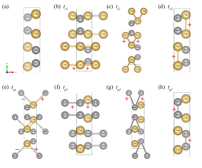
Figure S3: (a) Unit cell of minimum effective model of Ta₂Ni₃Te₅. (b)-(h) Hoppings considered in effective model. The hoppings are represented by bonds between Ta and Ni atoms. And the plus and minus represent the positive and negative values of hoppings.