MagneticKP: A package for quickly constructing k$\cdot$p models of magnetic and non-magnetic crystals

Abstract

We propose an efficient algorithm to construct $\bm{k}\cdot\bm{p}$ effective Hamiltonians, which is much faster than the previously proposed algorithms. This algorithm is implemented in MagneticKP package. The package applies to both single-valued (spinless) and double-valued (spinful) cases, and it works for both magnetic and nonmagnetic systems. By interfacing with SpaceGroupIrep or MSGCorep packages, it can directly output the $\bm{k}\cdot\bm{p}$ Hamiltonian around arbitrary momentum and expanded to arbitrary order in $k$.

Program summary

Program title: MagneticKP

Licensing provisions: GNU General Public Licence 3.0

Programming language: Mathematica

External routines/libraries used: SpaceGroupIrep (Optional), MSGCorep (Optional)

Developer’s repository link: https://github.com/zhangzeyingvv/MagneticKP

Nature of problem: Construct $\bm{k}\cdot\bm{p}$ Hamiltonian for arbitrary magnetic space group

Solution method: Linear algebra, iterative algorithm to solve common null space of operators

1 Introduction

$\bm{k}\cdot\bm{p}$ modelling is widely used in the research of condensed matter physics. Such models describe the local band structure around certain momentum $\bm{K}$ in the Brillouin zone and take the form of a Taylor expansion in powers of $\bm{k}$, with $\bm{k}$ being the derivation from $\bm{K}$. The famous early examples include the Kohn-Luttinger model and the Kane model for studying semiconductor materials [1, 2]. In the past twenty years, with the development in two-dimensional materials and topological materials, $\bm{k}\cdot\bm{p}$ modelling has become a standard tool for studying their properties. In these materials, the physical responses are mostly determined by the electronic states around a few band extremal or degeneracy points, so $\bm{k}\cdot\bm{p}$ models are most suitable for their description. For example, many exotic properties of graphene can be understood from its 2D Dirac model obtained using $\bm{k}\cdot\bm{p}$ method [3]. $\bm{k}\cdot\bm{p}$ models have also been constructed to study other 2D semiconductors, such as transition-metal dichalcogenides and monolayers of group-IV or group-V elements [4, 5, 6, 7], to capture the band inversion topology such as in HgTe quantum wells [8], and to describe nodal states in topological semimetals, such as Weyl/Dirac points [9, 10, 11, 12], triple points [13, 14], and various nodal loops/surfaces [15, 16, 17, 18, 19].

In practice, a $\bm{k}\cdot\bm{p}$ model is usually constructed from symmetry constraint. The input information include the symmetry group of at the expansion point $\bm{K}$ and the symmetry information of the target band states at $\bm{K}$. Depending on the needs, the output model is expanded to a specified cutoff power of $k$. At present, there already exist a few packages, including kdotp-symmetry[20], Qsymm [21], kdotp-generator (based on kdotp-symmetry) [22] and Model-Hamiltonian [23], which can construct $\bm{k}\cdot\bm{p}$ Hamiltonians. All these packages are written in Python and use a similar algorithm, namely, the direct-product decomposition algorithm (DDA). In the DDA approach, each symmetry constraint is transformed to a set of linear equations, and one solves the null space of these equations by the standard linear algebra method. After going through all symmetry constraints, one obtains a collection of null spaces. The output model Hamiltonian is obtained by calculating the intersection of all the null spaces using the standard Zassenhaus algorithm [24], such that it satisfies all the symmetry constraints.

In this work, we propose an improved algorithm, which has been implemented in our MagneticKP package (written in Wolfram language). We term this algorithm as the iterative simplification algorithm (ISA). We show that compared with the DDA, ISA reduces the time complexity of constructing $\bm{k}\cdot\bm{p}$ Hamiltonians. The improvement increases with the symmetry group size, the model dimension, and the cutoff power in $k$. The main difference lies in the method to obtain the intersection of a collection of null spaces. As mentioned above, DDA uses the direct Gaussian elimination method, which is quite time consuming. Instead, ISA adopts an iterative method, such that the problem size is reduced at each step in obtaining the common null spaces of two operators. Besides the improvement in algorithm, the usage of Wolfram language in the MagneticKP package also helps to enhance the speed, since its handling of analytic calculation is more efficient than Python. The application and the validity of our algorithm and package have been demonstrated in many of our previous works [25, 26, 27, 28].

This paper is organized as follows: In Sec. 2, we give a detailed description of ISA and compare it with DDA. In Sec. 3, we introduce the capabilities of MagneticKP package, including the installation and running of MagneticKP. In Sec. 4, we present a simple example. Finally, a conclusion is given in Sec. 5.

2 Algorithm

To construct a $\bm{k}\cdot\bm{p}$ Hamiltonian, we need to first specify the expansion point $\bm{K}$ and the basis states at $\bm{K}$. The form of the $\bm{k}\cdot\bm{p}$ Hamiltonian is constrained by the symmetry elements of the little co-group $G$ at $\bm{K}$. Consider a symmetry $Q\in G$. Its constraint on the Hamiltonian $H$ is given by

$$H(\bm{k})=\begin{cases}D(Q)H(R^{-1}\bm{k})D^{-1}(Q)&\text{if }Q=\{R|t\}\\ D(Q)H^{*}(-R^{-1}\bm{k})D^{-1}(Q)&\text{if }Q=\{R|t\}{\cal T}\\ \end{cases}$$ (1)

where the relation depends on whether $Q$ involves the time reversal operation $\mathcal{T}$, $D(Q)$ is the matrix (co)representation matrix of $Q$ (not necessarily irreducible) in the basis states. The target result is a Hamiltonian that satisfies symmetry constraints by all the $Q$’s in $G$ and meanwhile includes all the allowed terms. In the calculation, one does not need to go through all the $Q$’s. Only the generators of the magnetic little co-group at $\bm{K}$ are needed.

2.1 Problem formulation

Now, we formulate the above problem into a form that can be handled numerically. Suppose we take $N$ basis states at $\bm{K}$, and we demand a model expanded to $P$-th power in $k$. We may first decompose the $\bm{k}\cdot\bm{p}$ Hamiltonian $H$ as a sum

$$H(\bm{k})=\sum_{m=0}^{P}\mathcal{H}_{m}(\bm{k}),$$ (2)

where each $\mathcal{H}_{m}$ includes terms that of $m$-th power in $k$. According to (1), the symmetry transforms $\bm{k}$ in a linear way, so each individual $\mathcal{H}_{m}$ would satisfy the symmetry constraint in (1). Therefore, we are allowed to consider each $\mathcal{H}_{m}$ separately.

Note that $H$ and $\mathcal{H}_{m}$’s are $N\times N$ complex Hermitian matrices. It is known that $N\times N$ complex Hermitian matrices form a vector space over $\mathbb{R}$, which has a dimension of $N^{2}$. We can choose $N^{2}$ basis for this vector space, and label them as $M_{\mu}$ with $\mu=1,\cdots,N^{2}$. For example, for $N=2$, the four basis may be chosen as the identity matrix and the three Pauli matrices; for $N=3$, one may choose the identity and the eight Gell-Mann matrices, and so on.

After choosing the basis $M_{\mu}$, we can express the Hamiltonian $\mathcal{H}_{m}(\bm{k})$ in the following form

$$\mathcal{H}_{m}(\bm{k}) =\sum_{\ell=1,..,L;\ \mu=1,..,N^{2}}c^{\ell\mu}p_{\ell}(\bm{k})M_{\mu}.$$ (3)

Here, $p_{\ell}(\bm{k})\in\{k_{x}^{a}k_{y}^{b}k_{z}^{c}|a+b+c=m;a,b,c\geq 0\}$ is a product of the $k$ vector components with a total power of $m$. There are totally $L=\frac{1}{2}(m+1)(m+2)$ such products. We label these products by $\ell$, which runs from $1$ to $L$. The expansion coefficients $c^{\ell\mu}\in\mathbb{R}$ are what we want to find after imposing the symmetry constraints.

First, consider the first line in (1), i.e., for the case when $Q=\{R|t\}$ not involving $\mathcal{T}$. Note that the $D$ matrix does not depend on $\bm{k}$. Then the right hand of Eq. (1) (for $\mathcal{H}_{m}$) can be expressed as

$$D(Q)\mathcal{H}_{m}(R^{-1}\bm{k})D^{-1}(Q)=\sum_{\ell,n=1,\dots,L;\mu,\nu=1,..,N^{2}}c^{n\mu}p_{\ell}(\bm{k})F^{\ell}_{\ n}(Q)M_{\nu}J_{\ \mu}^{\nu}(Q).$$ (4)

Here, $F^{\ell}_{\ n}(Q)$ is an $L\times L$ constant matrix satisfying $p_{n}(R^{-1}\bm{k})=\sum_{\ell}p_{\ell}(\bm{k})F^{\ell}_{\ n}$; and $J_{\ \mu}^{\nu}(Q)$ is an $N^{2}\times N^{2}$ matrix satisfying $DM_{\mu}D^{-1}=\sum_{\nu}M_{\nu}J_{\ \mu}^{\nu}$. Then, the symmetry condition in (1) can be re-written in the following form

$$\mathbf{0}= \mathcal{H}_{m}(\bm{k})-D(Q)\mathcal{H}_{m}(R^{-1}\bm{k})D^{-1}(Q)$$ (5)

$$= \sum_{\ell,n=1,\dots,L;\mu,\nu=1,..,N^{2}}p_{\ell}(\bm{k})M_{\nu}\Big{[}\delta^{\ell}_{\ n}\delta_{\ \mu}^{\nu}-F^{\ell}_{\ n}(Q)J^{\nu}_{\ \mu}(Q)\Big{]}c^{n\mu}$$

$$= \mathbf{b}\cdot\mathbf{S}(Q)\cdot\mathbf{c}$$

where $\mathbf{b}\equiv(p_{1}M_{1},p_{1}M_{2}\cdots,p_{L}M_{N^{2}})$ is a $1\times LN^{2}$ row vector, $\mathbf{c}\equiv(c^{11},\cdots,c^{LN^{2}})^{T}$ is a $LN^{2}\times 1$ column vector, and

$$\mathbf{S}(Q)\equiv\delta^{\ell}_{\ n}\delta_{\ \mu}^{\nu}-F^{\ell}_{\ n}(Q)J^{\nu}_{\ \mu}(Q)$$ (6)

is an $LN^{2}\times LN^{2}$ matrix. Since $\mathbf{b}$ is a vector of linearly independent $k$-products, the condition in (5) is equivalent to

$$\mathbf{S}(Q)\ \mathbf{c}=\mathbf{0}.$$ (7)

Thus, $\mathbf{c}\in\mathrm{ker}\ \mathbf{S}(Q)$, so the condition reduces to finding the null space or the kernel of $\mathbf{S}(Q)$.

As for the second line in Eq. (1), i.e., for $Q=\{R|t\}{\cal T}$, one can see that we only need to slightly modify the definition of $\mathbf{S}(Q)$ as

$$\mathbf{S}(Q)\equiv\delta^{\ell}_{\ n}\delta_{\ \mu}^{\nu}-\tilde{F}^{\ell}_{\ n}(Q)\tilde{J}_{\ \mu}^{\nu}(Q),$$ (8)

where $\tilde{F}^{\ell}_{\ n}(Q)$ is defined from the relation $p_{n}(-R^{-1}\bm{k})=\sum_{\ell}p_{\ell}(\bm{k})\tilde{F}^{\ell}_{\ n}$; and $\tilde{J}^{\nu}_{\ \mu}(Q)$ satisfies $DM_{\mu}^{*}D^{-1}=\sum_{\nu}M_{\nu}\tilde{J}_{\ \mu}^{\nu}$.

Typically, the group $G$ has multiple generators $Q_{1},Q_{2},\cdots$. Each generator $Q_{i}$ gives a $\mathbf{S}(Q_{i})$ for which we solve its null space $\mathrm{ker}\ \mathbf{S}(Q_{i})$. The final solution is their common subspace $\mathfrak{S}=\bigcap_{i}\mathrm{ker}\ \mathbf{S}(Q_{i})$. In practice, we need to solve out a basis set $\{\mathbf{u}_{1},\cdots,\mathbf{u}_{r}\}$ for $\mathfrak{S}$, where $r=\text{dim}\mathfrak{S}$, such that the coefficient $c^{\ell\mu}$ in Eq. (3) is expressed as

$$c^{\ell\mu}=\sum_{i=1}^{r}a^{i}[\mathbf{u}_{i}]^{\ell\mu}$$ (9)

with $r$ real coefficients $a^{i}$ serving as the model parameters for $\mathcal{H}_{m}$.

2.2 Iterative simplification algorithm

The direct way to obtain the common null space $\mathfrak{S}$ is by the Gaussian elimination method. Here, we propose an iterative numerical method. To this end, we need to first introduce a definition, a proposition and a short proof.

Definition 1

$S$ is a linear mapping from $\mathbb{C}^{m}$ to $\mathbb{C}^{n}$. The matrix for $S$ in the standard bases is denoted as $\mathbf{S}$, which is of size $n\times m$. Let $\{\alpha_{1},\alpha_{2},\cdots,\alpha_{r}\}$ be any basis set for $\mathrm{ker}\,\mathbf{S}$, i.e., $\mathrm{ker}\,\mathbf{S}=\mathrm{Span}\{\alpha_{1},\alpha_{2},...,\alpha_{r}\}$, $r=\mathrm{dim}\,\mathrm{ker}\,\mathbf{S}$. Then, we define a $m\times r$ matrix $\mathcal{K}(\mathbf{S})$ associated with $\mathbf{S}$ by

$$\mathcal{K}(\mathbf{S})=(\alpha_{1},\alpha_{2},...,\alpha_{r}).$$

When treating each column of $\mathcal{K}(\mathbf{S})$ as a vector in $\mathbb{C}^{m}$, we can write

$$\mathrm{ker}\,\mathbf{S}=\mathrm{Span}\{\mathcal{K}(\mathbf{S})\}.$$

Proposition 1

Consider two linear mappings $A:\mathbb{C}^{m}\rightarrow\mathbb{C}^{n}$ and $B:\mathbb{C}^{m}\rightarrow\mathbb{C}^{p}$. The matrices for ${A}$ and ${B}$ in standard bases are $\mathbf{A}$ and $\mathbf{B}$, which are of size $n\times m$ and $p\times m$, respectively. Then, we have

$$\mathrm{ker}\,\mathbf{A}\bigcap\mathrm{ker}\,\mathbf{B}=\mathrm{Span}\big{\{}\mathcal{K}(\mathbf{A})\cdot\mathcal{K}(\mathbf{B}\cdot\mathcal{K}(\mathbf{A}))\big{\}}.$$

Proof: The intersection space of $\ker A$ and $\ker B$ is equal to the kernel of linear mapping restricted to the space $\ker A$, i.e. $\ker A\cap\ker B=\ker(B|_{\ker A})$. Now, take a set of bases of $\ker\mathbf{A}:$ $\{\alpha_{1},\alpha_{2},...,\alpha_{r}\}$ and let $\mathcal{K}(\mathbf{A})=(\alpha_{1},\alpha_{2},...,\alpha_{r})$ being a $m\times r$ matrix. The linear mapping $B|_{\ker A}:$ $\ker A\rightarrow\mathbb{C}^{n}$ in the basis of $\{\alpha_{1},\alpha_{2},...,\alpha_{r}\}$ is represented by the $p\times r$ matrix $\mathbf{B}\cdot\mathcal{K}(\mathbf{A})$. Then the $r\times\ell$ matrix $\mathcal{K}(\mathbf{B}\cdot\mathcal{K}(\mathbf{A}))$ gives the basis set of $\ker A\bigcap\ker B$ expressed in the basis of $\{\alpha_{1},\alpha_{2},...,\alpha_{r}\}$, where $\ell=\mathrm{dim}(\ker A\cap\ker B)$. The multiplication of $\mathcal{K}(\mathbf{A})$ from the left converts them back to the standard bases, which generates the desired result.

As we have discussed in the last subsection, the target is to find a basis set for the common null subspace $\mathfrak{S}=\bigcap_{i=1}^{s}\mathrm{ker}\ \mathbf{S}(Q_{i})$, where $s$ is the number of generators of $G$. Based on the above proposition, we can obtain it in the following iterative way. Let $\mathcal{U}_{1}=\mathcal{K}(\mathbf{S}(Q_{1}))$, and for $1\leq i\leq s-1$,

$$\mathcal{U}_{i+1}=\mathcal{U}_{i}\cdot\mathcal{K}(\mathbf{S}(Q_{i+1})\cdot\mathcal{U}_{i})$$ (10)

Then the final matrix $\mathcal{U}_{s}=(\mathbf{u}_{1},\cdots,\mathbf{u}_{r})$ contains the desired basis set for $\mathfrak{S}$.

The pseudo code for obtaining $\mathcal{U}_{s}$ is shown in Algorithm 1.

Algorithm 1 Iterative calculation of $\mathcal{U}_{s}$

procedure $\mathcal{U}$({$\mathbf{S}(Q_{1}),...,\mathbf{S}(Q_{s})$})

     $\mathcal{U}\leftarrow\mathcal{K}(\mathbf{S}(Q_{1}))$

     for $\mathbf{S}$ in {$\mathbf{S}(Q_{2}),...,\mathbf{S}(Q_{s})$} do

         if $\mathcal{U}=\varnothing$ then return $\varnothing$          

         $\mathcal{U}\leftarrow\mathcal{U}\cdot\mathcal{K}(\mathbf{S}\cdot\mathcal{U})$      return $\mathcal{U}$

2.3 Comparison of ISA to DDA

DDA differs from ISA in the way to obtain the common null space basis set, i.e., the $\mathcal{U}_{s}$ above. In DDA, after constructing $\mathbf{S}(Q_{i})$ $(i=1,\cdots,s)$, one needs to first solve the null space matrix $\mathcal{K}(\mathbf{S}(Q_{i}))$ for each $i$ separately. Then, $\mathcal{U}_{s}$ is obtained by combining all the $\mathcal{K}(\mathbf{S}(Q_{i}))$’s into one big matrix and do Gaussian elimination to find the common basis set [20]. Hence, it is a two-step process.

In comparison, in ISA, $\mathcal{U}_{s}$ is obtained in an iterative way. The dimension of space, i.e., the size of matrix, decreases in each iteration step, which greatly reduces the computational cost. The processes of the two algorithms are illustrated in Fig. 1.

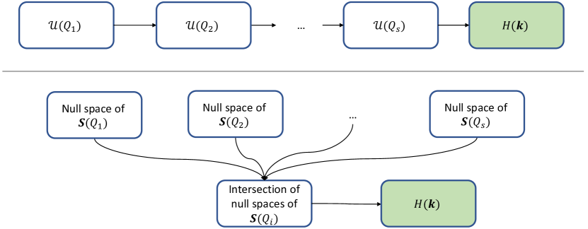
Figure 1: Schematic comparison of the two algorithms. Upper panel: ISA. Lower panel: DDA.

Here, we give an estimation of the time complexity of the two algorithms. The complexity for calculating the null space of a $a\times b$ $(a\geq b)$ matrix is approximately $O(ab^{2})$ [29] (note that this is a very rough estimate, because the method for NullSpace in Wolfram language is automatically chosen by "CofactorExpansion", "DivisionFreeRowReduction" and "OneStepRowReduction", thus the complexity of NullSpace also depends on the specific form of the matrix). The time complexity for finding $\mathcal{U}_{s}$ in DDA is about $O(s(LN^{2})^{3}+(\sum_{i=1}^{s}d_{i})\times(LN^{2})^{2})$, where $d_{i}=\mathrm{dim}\ker\mathbf{S}(Q_{i})$. The first term is for calculating the null spaces for the $s$ matrices $\mathbf{S}(Q_{i})$, and the second term is for calculating their intersection. In comparison, for ISA, the time complexity is approximately $O((LN^{2})^{3}+LN^{2}\sum_{n=2}^{s}(LN^{2}-\sum_{i=1}^{n}r_{i})^{2})$, where $r_{i}$ is the number of columns of $\mathcal{U}_{i}$. In practice, we find the first term dominates, so ISA complexity is roughly $O((LN^{2})^{3})$, which is at least $s$ times faster than DDA.

To test the computational efficiency, we construct several $\bm{k}\cdot\bm{p}$ Hamiltonians using three different ways: (1) ISA implemented in MagneticKP (written in Wolfram language), (2) DDA implemented in MagneticKP (written in Wolfram language), and (3) DDA implemented in kdotp-symmetry (written in Python language). The test results as shown in Table 1. One can see that ISA implemented in MagneticKP has the best performance. The time cost difference between approaches (1) and (3) becomes more and more pronounced with the cutoff power and basis size. One also notes that approach (2) is also much better than (3), which demonstrates that for the current task involving analytic calculations, Wolfram language is more efficient than Python.

Table 1: Comparison of time costs for three different approaches. The column labeled "MSG" gives the magnetic space group number. "corep" gives the $\Gamma$ label of the co-representation (basis size), "dim" is the dimension of the co-representation, "$k$-order" is the cutoff power of the $\bm{k}\cdot\bm{p}$ model. The three approaches are: (1) ISA implemented in MagneticKP, (2) DDA implemented in MagneticKP, and (3) DDA implemented in kdotp-symmetry. The values are in unit of second. All tests are run on intel i7-10870H CPU@2.20GHz with 32GB RAM.

MSG	corep	dim	$\bm{k}$-order	ISA (MagneticKP)	DDA (MagneticKP)	DDA (kdotp-symmetry)
226.123	$L_{4}L_{4}$	4	2	0.43	0.59	5.76
			4	1.18	3.20	137.99
			6	3.30	12.12	> 2 hours
			8	8.80	36.43	> 2 hours
218.82	$R_{4}R_{5}$	6	2	4.48	5.97	41.58
			4	10.22	22.80	490.33
			6	28.87	86.55	> 2 hours
			8	87.87	282.83	> 2 hours

3 Capability of MagneticKP

3.1 Installation

The steps of installing MagneticKP is exactly the same as installing MagneticTB [30]. One just needs to unzip the "MagneticKP-main.zip" file and copy the MagneticKP directory to any directory in $Path. e.g., copy to FileNameJoin[{$UserBaseDirectory, "Applications"}]. Then, one can start to use the package after running Needs["MagneticKP‘"]. The version of Mathematica should be $\geq$ v11.3.

3.2 Running

3.2.1 Core module

The core part of MagneticKP package is the function kpHam which computes the $\bm{k}\cdot\bm{p}$ Hamiltonian. The format of this function is

⬇

kpHam[korder, input, "Method"->"IterativeSimplification" or "DirectProductDecomposition"]

Here, korder can be both an integer or a list of integers that specifies the cutoff power in $k$ for the $\bm{k}\cdot\bm{p}$ Hamiltonian to be calculated. When korder is a list such as $\{n,m\}$, the function will output two Hamiltonians of the cutoff power of $n$ and $m$, respectively. input has the format of an Association in Mathematica. It contains the input information for constructing the Hamiltonian. There are three necessary inputs, the rotation part of $Q$, the (co)representation matrix of $Q$, and whether $Q$ is an unitary or an anti-unitary operator. The format of input is

⬇

input = <|

"Unitary" -><|$Q_{1}$ -> {$D(Q_{1})$, $R_{1}\bm{k}$},…|>,

"Anitunitary" -><|$Q_{2}$ -> {$D(Q_{2})$, -$R_{2}\bm{k}$},…|>

|>

Notice that the role of Keys of input["Unitary"] or input["Anitunitary"] is to make the input clearer, MagneticKP will respectively read the Values of input["Unitary"] and input["Anitunitary"] to do the calculation. $R\bm{k}$ can be in either Cartesian or primitive coordinates.

The default method in kpHam is ISA. Users can explicitly specify a method by putting "Method"->"IterativeSimplification" or "Method"->"DirectProductDecomposition" in kpHam. After the above parameters are set appropriately, one can run kpHam to obtain the $\bm{k}\cdot\bm{p}$ Hamiltonian. The output of kpHam is also an Association. The format of the output is [see Sec. 4 for a concrete example]

⬇

<|"ham" -> expression of $\bm{k}\cdot\bm{p}$ Hamiltonian, "korder" -> order of Hamiltonian,

"dim" -> dimension of Hamiltonian, "NumberOfParameters" -> number of parameters|>

3.2.2 IO module

The input to kpHam contains the matrix $D(Q_{i})$. Here, we introduce how to get its expression. In general, for $Q_{i}\in G$, one can use the projective representation method to get the irreducible representation $\Delta(Q_{i})$. The reality of $\Delta(Q_{i})$ can be determined by Herring’s rule [31] and $D(Q_{i})$ can be easily constructed from $\Delta(Q_{i})$ and the reality of $\Delta(Q_{i})$ [32]. More direct method is to obtain $D(Q_{i})$ from standard reference books [33, 32, 34, 35], or Bilbao crystallographic server [36], or many software packages [37, 38, 39, 40, 41]. Here, we provide a function interfaceRep to interface with packages SpaceGroupIrep [41] and MSGCorep [42]. MSGCorep package is our home-made package and will be made public soon. The format of interfaceRep is

⬇

interfaceRep[MSGNO, k, reps, "CartesianCoordinates" -> True or False, "CalculateGenerators" -> True or False]

where MSGNO can be either space group number (one integer) or BNS magnetic space group number (a list containing two integers). When MSGNO is an integer number (list), SpaceGroupIrep (MSGCorep) package must be loaded. k can be given in the form of the coordinate of $\bm{K}$ or the symbol of the $\bm{K}$ point (if it is a high-symmetry point). reps is an integer or a list of integers, which represents the serial number of irreducible (co)representations in showLGIrepTab(showMLGCorep). When reps is a list, MagneticKP will automatically calculate the direct sum of (co)representations. "CartesianCoordinates" (default value is True) tells MagneticKP whether to convert the operations into Cartesian coordinates. Finally, since SpaceGroupIrep (MSGCorep) will show all the symmetry operations in the (magnetic) little group, to save the computing resources we develop a greedy algorithm to find the generators of a group [43]. The pseudo code is shown in Algorithm 2.

Algorithm 2 Use greedy algorithm to find the generators of a group

procedure getGenerator(InputGroup)

     Generator $\leftarrow$ $\varnothing$

     group $\leftarrow$ {identity element}

     for element in InputGroup do

         temGenerator $\leftarrow$ Append[Generator,element]

         temgroup $\leftarrow$ GenerateGroup[temGenerator]

         if group $\neq$ temgroup then Generator $\leftarrow$ temGenerator;

              group $\leftarrow$ temgroup          

         if group $=$ InputGroup then Break               return Generator

It should be mentioned that Ref. [22, 44] only generate models for high symmetry $\bm{k}$ points. In comparison, in MagneticKP, with the help of SpaceGroupIrep (MSGCorep), it can work for arbitrary $\bm{k}$ point, for arbitrary direct sums of more than two irreducible representations, for different types of coordinates etc. Hence, it is also more general and more convenient than previous packages.

4 Example

We use the four-band nodal ring in TiB₂ [25] as an example to show how to use MagneticKP. TiB₂ is a nonmagnetic material with time-reversal symmetry and belongs to space group 191 ($P6/mmm$) (see Fig. 2(a)). The four-band nodal ring appears around $K\ (-\frac{1}{3},\frac{2}{3},0)$ point when spin-orbit coupling effect is neglected. The generators of the little co-group at $K$ can be chosen as $\{C_{3}^{+}|000\}$, $\{C_{2}^{\prime\prime}|000\}$, $\{\sigma_{h}|000\}$ and $\{I{\cal T}|000\}$. Then $R\bm{k}$ and the single-value representation matrices of the relevant band representations ($K_{5}\oplus K_{6}$) can be written as [32]:

$$C_{3}^{+}:(k_{x},k_{y},k_{z}) \rightarrow(-\frac{k_{x}}{2}-\frac{\sqrt{3}k_{y}}{2},\frac{\sqrt{3}k_{x}}{2}-\frac{k_{y}}{2},k_{z}), D(C_{3}^{+})=-\frac{\Gamma_{0,0}}{2}-\frac{1}{2}i\sqrt{3}\Gamma_{3,2}$$ (11)

$$C_{2}^{\prime\prime}:(k_{x},k_{y},k_{z}) \rightarrow(k_{x},-k_{y},k_{z}), D(C_{2}^{\prime\prime})=\Gamma_{0,3}$$

$$\sigma_{h}:(k_{x},k_{y},k_{z}) \rightarrow(k_{x},k_{y},-k_{z}), D(\sigma_{h})={\Gamma_{3,0}}$$

$$I{\cal T}:(k_{x},k_{y},k_{z}) \rightarrow(k_{x},k_{y},k_{z}), D(I{\cal T})=\Gamma_{0,0}$$

where $\Gamma_{i,j}=\sigma_{i}\otimes\sigma_{j}$, $\sigma_{0}$ is the $2\times 2$ identity matrix and $\sigma_{i}(i=1,2,3)$ are the three Pauli matrices. With these input information, one can run the following code to get the $\bm{k}\cdot\bm{p}$ Hamiltonian up to first order

⬇

1Needs["MagneticKP‘"];

2input=<|"Unitary" -> <|

3C3 -> {-IdentityMatrix[4]/2 + I Sqrt[3] KroneckerProduct[PauliMatrix[3], PauliMatrix[2]]/2, {-kx/2 - (Sqrt[3] ky)/2, Sqrt[3] kx/2 - ky/2, kz}},

4C2 -> {KroneckerProduct[PauliMatrix[0], PauliMatrix[3]], {-kx, ky, -kz}},

5$\sigma$h -> {KroneckerProduct[PauliMatrix[3], PauliMatrix[0]], {kx, ky, -kz}}|>,

6"Anitunitary" -> <|IT -> {IdentityMatrix[4], {kx, ky, kz}}|>|>;

7MatrixForm[kpHam[1, input]["ham"]]

The output of the above script is:

Here, $C_{i,j}$ is the $j$-th real parameter of the $i$-th $\bm{k}$-order of the $\bm{k}\cdot\bm{p}$ Hamiltonian. On the $k_{z}=0$ plane, the Hamiltonian is decoupled into two $2\times 2$ diagonal blocks, which has different mirror eigenvalues ($+1$ for $K_{5}$ and $-1$ for $K_{6}$) and makes it possible to generate a nodal ring on the $k_{z}=0$ plane. To fully capture the four-band nodal ring in TiB₂ [25], one needs a $2$nd order Hamiltonian, which can be easily obtained by changing line 7 in the above script to

⬇

MatrixForm[kpHam[2, input]["ham"]]

The band structure of the 2nd order $\bm{k}\cdot\bm{p}$ Hamiltonian is shown in Fig. 2(b), which is consistent with the result in Ref. [25].

A more direct way is to interface with MSGCorep. One needs to simply write

⬇

Needs["MSGCorep‘"]

input = interfaceRep[{191, 234}, "K", {5, 6}];

kpHam[2, input]

Here, the output of interfaceRep is:

This output additionally contains the labels of (co)representations, which would make the analysis more convenient.

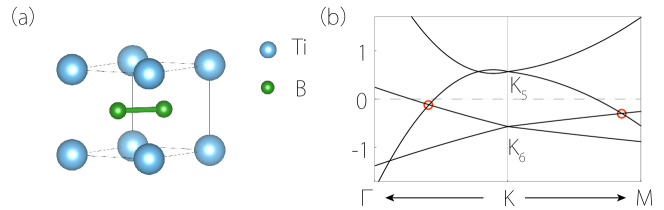
Figure 2: (a) Crystal structure of TiB₂. (b) Band structure of the output of kpHam[2, input]. Here, we take the values $C_{0,1}=0,C_{0,2}=0.6,C_{2,1}=0,C_{2,2}=0.13,C_{2,3}=0.,C_{2,4}=0.12,C_{2,5}=0,C_{2,6}=0,C_{2,7}=0,C_{1,1}=0.1,C_{1,2}=0,C_{1,3}=0$. The two red circles indicate the crossing points on the nodal ring.

5 Conclusion

In conclusion, we have developed a package MagneticKP to generate $\bm{k}\cdot\bm{p}$ Hamiltonian at an arbitrary momentum point. We develop the ISA approach, which is much faster than the algorithm used in previous packages. By interfacing with SpaceGroupIrep (MSGCorep), MagneticKP can generate the $\bm{k}\cdot\bm{p}$ Hamiltonians for any (magnetic) space group. The package will be a useful tool for band structure modeling and analysis.

References

- Luttinger and Kohn [1955] J. M. Luttinger, W. Kohn, Motion of Electrons and Holes in Perturbed Periodic Fields, Physical Review 97 (1955) 869.
- Kane [1957] E. O. Kane, Band structure of indium antimonide, Journal of Physics and Chemistry of Solids 1 (1957) 249–261.
- Castro Neto et al. [2009] A. H. Castro Neto, F. Guinea, N. M. R. Peres, K. S. Novoselov, A. K. Geim, The electronic properties of graphene, Reviews of Modern Physics 81 (2009) 109–162.
- Liu et al. [2011a] C.-C. Liu, W. Feng, Y. Yao, Quantum Spin Hall Effect in Silicene and Two-Dimensional Germanium, Physical Review Letters 107 (2011a) 076802.
- Liu et al. [2011b] C.-C. Liu, H. Jiang, Y. Yao, Low-energy effective Hamiltonian involving spin-orbit coupling in silicene and two-dimensional germanium and tin, Physical Review B 84 (2011b) 195430.
- Xiao et al. [2012] D. Xiao, G.-B. Liu, W. Feng, X. Xu, W. Yao, Coupled Spin and Valley Physics in Monolayers of MoS2 and Other Group-VI Dichalcogenides, Physical Review Letters 108 (2012) 196802.
- Lu et al. [2016] Y. Lu, D. Zhou, G. Chang, S. Guan, W. Chen, Y. Jiang, J. Jiang, X.-s. Wang, S. A. Yang, Y. P. Feng, Y. Kawazoe, H. Lin, Multiple unpinned Dirac points in group-Va single-layers with phosphorene structure, npj Computational Materials 2 (2016) 16011.
- Bernevig et al. [2006] B. A. Bernevig, T. L. Hughes, S.-C. Zhang, Quantum Spin Hall Effect and Topological Phase Transition in HgTe Quantum Wells, Science 314 (2006) 1757.
- Wan et al. [2011] X. Wan, A. M. Turner, A. Vishwanath, S. Y. Savrasov, Topological semimetal and Fermi-arc surface states in the electronic structure of pyrochlore iridates, Phys. Rev. B 83 (2011) 205101.
- Wang et al. [2012] Z. Wang, Y. Sun, X.-Q. Chen, C. Franchini, G. Xu, H. Weng, X. Dai, Z. Fang, Dirac semimetal and topological phase transitions in ABi (A=Na, K, Rb), Physical Review B 85 (2012) 195320.
- Yang and Nagaosa [2014] B.-J. Yang, N. Nagaosa, Classification of stable three-dimensional Dirac semimetals with nontrivial topology, Nature Communications 5 (2014) ncomms5898.
- Young and Kane [2015] S. M. Young, C. L. Kane, Dirac Semimetals in Two Dimensions, Physical Review Letters 115 (2015) 126803.
- Weng et al. [2016] H. Weng, C. Fang, Z. Fang, X. Dai, Topological semimetals with triply degenerate nodal points in -phase tantalum nitride, Physical Review B 93 (2016) 241202.
- Zhu et al. [2016] Z. Zhu, G. W. Winkler, Q. Wu, J. Li, A. A. Soluyanov, Triple Point Topological Metals, Physical Review X 6 (2016) 031003.
- Yang et al. [2014] S. A. Yang, H. Pan, F. Zhang, Dirac and Weyl Superconductors in Three Dimensions, Phys. Rev. Lett. 113 (2014) 046401.
- Weng et al. [2015] H. Weng, Y. Liang, Q. Xu, R. Yu, Z. Fang, X. Dai, Y. Kawazoe, Topological node-line semimetal in three-dimensional graphene networks, Physical Review B 92 (2015) 045108.
- Zhao et al. [2016] Y. X. Zhao, A. P. Schnyder, Z. Wang, Unified Theory of P T and C P Invariant Topological Metals and Nodal Superconductors, Physical Review Letters 116 (2016).
- Bzdušek and Sigrist [2017] T. Bzdušek, M. Sigrist, Robust doubly charged nodal lines and nodal surfaces in centrosymmetric systems, Phys. Rev. B 96 (2017) 155105.
- Wu et al. [2018] W. Wu, Y. Liu, S. Li, C. Zhong, Z.-M. Yu, X.-L. Sheng, Y. X. Zhao, S. A. Yang, Nodal surface semimetals: Theory and material realization, Physical Review B 97 (2018) 115125.
- Gresch [2018] D. Gresch, Identifying Topological Semimetals, Ph.D. thesis (ETH Zurich) (2018).
- Varjas et al. [2018] D. Varjas, T. . Rosdahl, A. R. Akhmerov, Qsymm: algorithmic symmetry finding and symmetric Hamiltonian generation, New Journal of Physics 20 (2018) 093026.
- Jiang et al. [2021] Y. Jiang, Z. Fang, C. Fang, A kp Effective Hamiltonian Generator, Chin. Phys. Lett. 38 (2021) 077104.
- Zhan et al. [2021] G. Zhan, M. Shi, Z. Yang, H. Zhang, A Programmable k $\cdotp$ p Hamiltonian Method and Application to Magnetic Topological Insulator MnBi2Te4, Chinese Physics Letters 38 (2021) 077105.
- Luks et al. [1997] E. M. Luks, F. Rákóczi, C. R. Wright, Some Algorithms for Nilpotent Permutation Groups, Journal of Symbolic Computation 23 (1997) 335–354.
- Zhang et al. [2017] X. Zhang, Z.-M. Yu, X.-L. Sheng, H. Y. Yang, S. A. Yang, Coexistence of four-band nodal rings and triply degenerate nodal points in centrosymmetric metal diborides, Physical Review B 95 (2017) 235116.
- Yu et al. [2022] Z.-M. Yu, Z. Zhang, G.-B. Liu, W. Wu, X.-P. Li, R.-W. Zhang, S. A. Yang, Y. Yao, Encyclopedia of emergent particles in three-dimensional crystals, Science Bulletin 67 (2022) 375–380.
- Liu et al. [2022] G.-B. Liu, Z. Zhang, Z.-M. Yu, S. A. Yang, Y. Yao, Systematic investigation of emergent particles in type-III magnetic space groups, Physical Review B 105 (2022) 085117.
- Zhang et al. [2022] Z. Zhang, G.-B. Liu, Z.-M. Yu, S. A. Yang, Y. Yao, Encyclopedia of emergent particles in type-IV magnetic space groups, Physical Review B 105 (2022) 104426.
- Hogben [2006] L. Hogben (Ed.), Handbook of Linear Algebra, 2006.
- Zhang et al. [2022] Z. Zhang, Z.-M. Yu, G.-B. Liu, Y. Yao, MagneticTB: A package for tight-binding model of magnetic and non-magnetic materials, Computer Physics Communications 270 (2022) 108153.
- Herring [1937] C. Herring, Effect of Time-Reversal Symmetry on Energy Bands of Crystals, Physical Review 52 (1937) 361.
- Bradley and Cracknell [2009] C. Bradley, A. Cracknell, Mathematical theory of symmetry in solids: representation theory for point groups and space groups, Oxford classic texts in the physical sciences, Oxford, 2009.
- Bradley and Davies [1968] C. J. Bradley, B. L. Davies, Magnetic Groups and Their Corepresentations, Reviews of Modern Physics 40 (1968) 359–379.
- Lax [2001] M. Lax, Symmetry Principles in Solid State and Molecular Physics, 2001.
- Dresselhaus et al. [2008] M. S. Dresselhaus, G. Dresselhaus, A. Jorio, Group theory: application to the physics of condensed matter, Berlin, 2008.
- Aroyo et al. [2006] M. I. Aroyo, A. Kirov, C. Capillas, J. M. Perez-Mato, H. Wondratschek, Bilbao Crystallographic Server. II. Representations of crystallographic point groups and space groups, Acta Crystallographica Section A 62 (2006) 115–128.
- Bosma et al. [1997] W. Bosma, J. Cannon, C. Playoust, The Magma Algebra System I: The User Language, Journal of Symbolic Computation 24 (1997) 235–265.
- Iraola et al. [2020] M. Iraola, J. L. Mañes, B. Bradlyn, T. Neupert, M. G. Vergniory, S. S. Tsirkin, IrRep: symmetry eigenvalues and irreducible representations of ab initio band structures, arXiv:2009.01764 [cond-mat, physics:physics] (2020).
- Matsugatani et al. [2021] A. Matsugatani, S. Ono, Y. Nomura, H. Watanabe, qeirreps: An open-source program for Quantum ESPRESSO to compute irreducible representations of Bloch wavefunctions, Computer Physics Communications 264 (2021) 107948.
- noa [2021] GAP – Groups, Algorithms, and Programming, Version 4.11.1, 2021.
- Liu et al. [2021] G.-B. Liu, M. Chu, Z. Zhang, Z.-M. Yu, Y. Yao, SpaceGroupIrep: A package for irreducible representations of space group, Computer Physics Communications 265 (2021) 107993.
- Liu and et al. [2021] G.-B. Liu, et al., MSGCorep: A package for corepresentations of magnetic space groups, to be published. (2021).
- Cormen [2001] T. H. Cormen (Ed.), Introduction to algorithms, Cambridge, Mass, 2001.
- Tang and Wan [2021] F. Tang, X. Wan, Exhaustive constructions of effective models in 1651 magnetic space groups, Physical Review B 104 (2021) 085137.