Consistency study of high- and low-accreting Mg ii quasars:
No significant effect of the Fe ii to Mg ii flux ratio on the radius-luminosity relation dispersion

Narayan Khadka\scalerel |1\scalerel |1{}^{\href https://orcid.org/0000-0001-5512-27161}, Michal Zajaček\scalerel |2\scalerel |2{}^{\href https://orcid.org/0000-0001-6450-11872}, Swayamtrupta Panda\scalerel |3,4\scalerel |34{}^{\href https://orcid.org/0000-0002-5854-7426{3,4}},   Mary Loli Martínez-Aldama\scalerel |5\scalerel |5{}^{\href https://orcid.org/0000-0002-7843-7689{5}}, Bharat Ratra\scalerel |1\scalerel |1{}^{\href https://orcid.org/0000-0002-7307-07261}
1Department of Physics, Kansas State University, 116 Cardwell Hall, Manhattan, KS 66506, USA
2Department of Theoretical Physics and Astrophysics, Faculty of Science, Masaryk University, Kotlářská 2, 611 37 Brno, Czech Republic
3Center for Theoretical Physics, Polish Academy of Sciences, Al. Lotników 32/46, 02-668 Warsaw, Poland
4Laboratório Nacional de Astrofísica - MCTIC, R. dos Estados Unidos, 154 - Nações, Itajubá - MG, 37504-364, Brazil
5Departamento de Astronomía, Universidad de Chile, Camino del Observatorio 1515, Santiago, Chile
E-mail: nkhadka@phys.ksu.eduE-mail: zajacek@mail.muni.czE-mail: panda@cft.edu.plCNPq fellowE-mail: mmartinez@das.uchile.clE-mail: ratra@phys.ksu.edu
(Accepted XXX. Received YYY; in original form ZZZ)
Abstract

We use observations of 66 reverberation-measured Mg ii quasars (QSOs) in the redshift range 0.36z1.6860.36𝑧1.6860.36\leq z\leq 1.686 — a subset of the 78 QSOs we previously studied that also have FeiisubscriptFeii{\cal R}_{\rm{Fe\textsc{ii}}} (flux ratio parameter of UV Fe ii to Mg ii that is used as an accretion-rate proxy) measurements — to simultaneously constrain cosmological model parameters and QSO 2-parameter and 3-parameter radius-luminosity (RL𝑅𝐿R-L) relation parameters in six different cosmological models. We find that these QSO RL𝑅𝐿R-L relation parameters are independent of the assumed cosmological model and so these QSOs are standardizable through the RL𝑅𝐿R-L relations. Also: (1) With the 2-parameter RL𝑅𝐿R-L relation, we find that the low-FeiisubscriptFeii{\cal R}_{\rm{Fe\textsc{ii}}} and high-FeiisubscriptFeii{\cal R}_{\rm{Fe\textsc{ii}}} data subsets obey the same RL𝑅𝐿R-L relation within the error bars. (2) Extending the 2-parameter RL𝑅𝐿R-L relation to a 3-parameter one does not result in the hoped-for reduction in the intrinsic dispersion of the RL𝑅𝐿R-L relation. (3) Neither of the 3-parameter RL𝑅𝐿R-L relations provide a significantly better fit to the measurements than does the 2-parameter RL𝑅𝐿R-L relation. These are promising results for the on-going development of Mg ii cosmological probes. The first and third of these results differ significantly from those we found elsewhere from analyses of reverberation-measured Hβ𝛽\beta QSOs.

keywords:
(cosmology:) cosmological parameters – (cosmology:) observations – (cosmology:) dark energy – (galaxies:) quasars: emission lines
pubyear: 2022pagerange: Consistency study of high- and low-accreting Mg ii quasars: No significant effect of the Fe ii to Mg ii flux ratio on the radius-luminosity relation dispersionA

1 Introduction

The spatially-flat ΛΛ\LambdaCDM model (Peebles, 1984) is consistent with most cosmological observations (see, e.g. Scolnic et al., 2018; Yu et al., 2018; Planck Collaboration, 2020; eBOSS Collaboration, 2021). This model assumes that the dark energy responsible for the currently accelerated cosmological expansion is a time-independent cosmological constant ΛΛ\Lambda that contributes 70%similar-toabsentpercent70\sim 70\% of the current cosmological energy budget, with non-relativistic cold dark matter (CDM) contributing 25%similar-toabsentpercent25\sim 25\%, and with most of the remaining 5%similar-toabsentpercent5\sim 5\% contributed by non-relativistic baryonic matter. However, observational data do not rule out a little spatial curvature or dynamical dark energy, so we also study such cosmological models in this paper.

Some measurements (of the same quantity) appear mutually incompatible when considered in the spatially-flat ΛΛ\LambdaCDM model (see, e.g. Di Valentino et al., 2021a; Perivolaropoulos & Skara, 2021; Abdalla et al., 2022). It is not clear whether these discrepancies point to new physics beyond the spatially-flat ΛΛ\LambdaCDM model or instead are a reflection of as yet unidentified systematic errors in one or both of the mutually incompatible data sets. New alternate cosmological probes might help resolve this issue. Such probes include H ii starburst galaxy observations which reach to redshift z2.4similar-to𝑧2.4z\sim 2.4 (Mania & Ratra, 2012; Chávez et al., 2014; González-Morán et al., 2021; Cao et al., 2020, 2021a, 2022c; Johnson et al., 2022; Mehrabi et al., 2022), quasar (QSO) angular size observations which reach to z2.7similar-to𝑧2.7z\sim 2.7 (Cao et al., 2017; Ryan et al., 2019; Cao et al., 2020, 2021b; Zheng et al., 2021; Lian et al., 2021), QSO X-ray and UV flux observations which reach to z7.5similar-to𝑧7.5z\sim 7.5 (Risaliti & Lusso, 2015, 2019; Khadka & Ratra, 2020a, b, 2021, 2022; Lusso et al., 2020; Rezaei et al., 2022; Luongo et al., 2021; Dainotti et al., 2022a),111Although the most recent Lusso et al. (2020) QSO flux compilation can only be used to derive significantly lower-z𝑧z cosmological constraints since it assumes a UV–X-ray correlation model that is invalid above z1.51.7similar-to𝑧1.51.7z\sim 1.5-1.7 (Khadka & Ratra, 2021, 2022). and gamma-ray burst observations that reach to z8.2similar-to𝑧8.2z\sim 8.2 (Wang et al., 2016, 2022; Fana Dirirsa et al., 2019; Demianski et al., 2021; Khadka & Ratra, 2020c; Khadka et al., 2021c; Hu et al., 2021; Luongo & Muccino, 2021; Cao et al., 2022d, e, a; Dainotti et al., 2022b).

Reverberation-measured QSOs might prove to be another useful cosmological probe. The method is based on the observed broad-line region (hereafter BLR) radius-luminosity (RL𝑅𝐿R-L) relation or rather correlation (Koratkar & Gaskell, 1991; Peterson, 1993; Kaspi et al., 2000; Bentz et al., 2013) that allows one to convert the measured rest-frame time-delay of the broad emission line with respect to the photoionizing continuum to an absolute monochromatic luminosity of the QSO.222For early discussions of reverberation-measured QSOs in cosmology, see Watson et al. (2011), Haas et al. (2011), and Czerny et al. (2013); more recent discussions can be traced back through Martínez-Aldama et al. (2019), Panda et al. (2019a), Martinez Aldama et al. (2020a), Zajaček et al. (2021), and Czerny et al. (2021). We have shown that the largest available compilation of 78 reverberation-measured Mg ii QSOs are standardizable through the observed 2-parameter RL𝑅𝐿R-L relation and that the current best Mg ii cosmological constraints are weak but consistent with those determined from better-established cosmological probes (Khadka et al., 2021b).333In our analyses we simultaneously determine cosmological-model and RL𝑅𝐿R-L-correlation parameters; this allows us to circumvent the circularity problem. We found that the QSO RL𝑅𝐿R-L relation is independent of the assumed cosmological model so these Mg ii QSOs are standardizable and, thus, useful for the purpose of constraining cosmological parameters.

More recently, we performed similar analyses using the largest available compilation of 118 Hβ𝛽\beta QSO sources, where we found that the 2-parameter RL𝑅𝐿R-L relation Hβ𝛽\beta cosmological constraints were somewhat (2σsimilar-toabsent2𝜎\sim 2\sigma) inconsistent with those from better-established cosmological probes (Khadka et al., 2021a). In contrast, we have found that cosmological parameters determined from the largest available data set of 38 high-quality C iv QSOs are consistent with those from better-established BAO+H(z)𝐻𝑧H(z) data as well as with those from Mg ii QSOs, which allows us to jointly analyze the C iv and Mg ii samples, as well as use the joint C iv+Mg ii+BAO+H(z)𝐻𝑧H(z) sample to constrain cosmological parameters (Cao et al., 2022b). Combining the C iv+Mg ii sample with the BAO+H(z)𝐻𝑧H(z) sample alters the cosmological constraints by 0.1σsimilar-toabsent0.1𝜎\sim 0.1\sigma at most in comparison with those from the BAO+H(z)𝐻𝑧H(z) sample alone.

To try to reduce the intrinsic dispersion of the QSO sample, attempts have previously been made to correct for the accretion-rate effect observed in the 2-parameter RL𝑅𝐿R-L relation (Du & Wang, 2019; Martínez-Aldama et al., 2020b; Zajaček et al., 2021; Prince et al., 2022) by extending it to a 3-parameter RL𝑅𝐿R-L relation. Partially to determine whether such a procedure might alter the Hβ𝛽\beta cosmological constraints, we also considered a 3-parameter RL𝑅𝐿R-L relation, with optical FeiisubscriptFeii{\cal R}_{\rm{Fe\textsc{ii}}} being the third parameter (Khadka et al., 2021a).444For Hβ𝛽\beta quasars, FeiisubscriptFeii{\cal R}_{\rm{Fe\textsc{ii}}} is the ratio of the flux densities of the optical Fe ii line to the Hβ𝛽\beta broad component, and analogously, for MgII sources, it is defined as the ratio of the flux densities of the UV Fe ii pseudocontinuum and the MgII broad line. FeiisubscriptFeii{\cal R}_{\rm{Fe\textsc{ii}}} is used as an accretion-rate intensity proxy. More interestingly, we confirmed that the low- and high-FeiisubscriptFeii{\cal R}_{\rm{Fe\textsc{ii}}} Hβ𝛽\beta sources obey significantly different RL𝑅𝐿R-L relations, which suggests that it might not be possible to standardize Hβ𝛽\beta QSOs using an RL𝑅𝐿R-L relation. We also discovered that the intrinsic dispersion did not significantly decrease when going from the 2- to the 3-parameter RL𝑅𝐿R-L relation. These findings motivated us to examine here the same issues for the Mg ii sources, whose cosmological constraints are compatible with those derived using better-established cosmological probes (Khadka et al., 2021b).

In this paper, we also investigate two 3-parameter RL𝑅𝐿R-L relations for Mg ii QSO sources, one in which the time-delay depends exponentially on FeiisubscriptFeii{\cal R}_{\rm{Fe\textsc{ii}}}, and the other where it depends on a power of FeiisubscriptFeii{\cal R}_{\rm{Fe\textsc{ii}}}. Our conclusions are qualitatively similar in the two 3-parameter cases. We find that for Mg ii data and the 2-parameter RL𝑅𝐿R-L relation, the low-FeiisubscriptFeii{\cal R}_{\rm{Fe\textsc{ii}}} and high-FeiisubscriptFeii{\cal R}_{\rm{Fe\textsc{ii}}} data subsets obey the same RL𝑅𝐿R-L relation within the error bars. This differs from what happens in the Hβ𝛽\beta case (Khadka et al., 2021a) and is a hopeful result for the on-going development of Mg ii cosmological probes. In the 3-parameter RL𝑅𝐿R-L relation cases, the inclusion of the third parameter increases the RL𝑅𝐿R-L relation parameter differences between the low-FeiisubscriptFeii{\cal R}_{\rm{Fe\textsc{ii}}} and high-FeiisubscriptFeii{\cal R}_{\rm{Fe\textsc{ii}}} data subsets. This increase is not very significant for the exponential FeiisubscriptFeii{\cal R}_{\rm{Fe\textsc{ii}}} case but is a little more significant for the power-law FeiisubscriptFeii{\cal R}_{\rm{Fe\textsc{ii}}} RL𝑅𝐿R-L relation. However, we find that extending the 2-parameter RL𝑅𝐿R-L relation to a 3-parameter does not reduce the intrinsic dispersion of the RL𝑅𝐿R-L relation,555This is similar to what happens in the Hβ𝛽\beta case (Khadka et al., 2021a). which was the main motivation for extending the 2-parameter RL𝑅𝐿R-L relation. In Khadka et al. (2021a) we found that for the full Hβ𝛽\beta data set the 3-parameter RL𝑅𝐿R-L relation provided a significantly better fit to the measurements than did the 2-parameter RL𝑅𝐿R-L relation, unlike what we find for Mg ii data here. This is because the Hβ𝛽\beta low-FeiisubscriptFeii{\cal R}_{\rm{Fe\textsc{ii}}} and high-FeiisubscriptFeii{\cal R}_{\rm{Fe\textsc{ii}}} data subsets obey very different 2-parameter RL𝑅𝐿R-L relations, unlike what we find for Mg ii data here.

In Sec. 2 we describe the dark energy cosmological models we use. In Sec. 3 we summarize the Mg ii QSO data we use to constrain cosmological-model and RL𝑅𝐿R-L correlation parameters. In Sec. 4 we summarize the data analysis methods we use. We present our results in Sec. 5, discuss some of them in more detail in Sec. 6, and conclude in Sec. 7.

2 Parameters and Cosmological models

In this study we use Mg ii QSOs to simultaneously infer cosmological model parameters 𝐩𝐩\mathbf{p} as well as the parameters of either the 2-parameter or the 3-parameter RL𝑅𝐿R-L correlation.

We use three pairs of dark-energy cosmological models with flat and non-flat spatial geometries, hence in total 6 cosmological models.666For discussions of constraints on spatial curvature see Chen et al. (2016), Rana et al. (2017), Ooba et al. (2018a, c), Park & Ratra (2019c, a), Wei (2018), DES Collaboration (2019), Li et al. (2020), Efstathiou & Gratton (2020), Di Valentino et al. (2021b), Vagnozzi et al. (2021a); Vagnozzi et al. (2021b), KiDS Collaboration (2021), Arjona & Nesseris (2021), Dhawan et al. (2021), Renzi et al. (2021), Geng et al. (2022), Wei & Melia (2022), Mukherjee & Banerjee (2022), and references therein. The cosmological expansion rate or the Hubble parameter H(z,𝐩)𝐻𝑧𝐩H(z,\mathbf{p}) is introduced for each cosmological model below as a function of the cosmological redshift z𝑧z and a set of cosmological parameters 𝐩𝐩\mathbf{p} specific to each model. H(z,𝐩)𝐻𝑧𝐩H(z,\mathbf{p}) is then used to make theoretical predictions for Mg ii QSOs, specifically their rest-frame BLR time delays τ𝜏\tau that are related to the BLR radius as R=cτ𝑅𝑐𝜏R=c\tau where c𝑐c is the speed of light.

The fundamental observables for each Mg ii QSO is its redshift z𝑧z, determined from the shift of its spectral lines, and the monochromatic flux density F3000subscript𝐹3000F_{3000} at 3000 Å  measured in ergs1cm2ergsuperscripts1superscriptcm2{\rm erg\,s^{-1}\,cm^{-2}}. To obtain the RL𝑅𝐿R-L relation for each cosmological model, we calculate the monochromatic luminosity at 3000 Å  using

L3000(z,𝐩)=4πDL(z,𝐩)2F3000,subscript𝐿3000𝑧𝐩4𝜋subscript𝐷𝐿superscript𝑧𝐩2subscript𝐹3000L_{3000}(z,\mathbf{p})=4\pi D_{L}(z,\mathbf{p})^{2}F_{3000}\,, (1)

where the luminosity distance DL(z,𝐩)subscript𝐷L𝑧𝐩D_{\rm L}(z,\mathbf{p}) (expressed in cm) is a function of z𝑧z and of the cosmological-model parameters 𝐩𝐩\mathbf{p}. Depending on the considered cosmological model and its current spatial curvature density parameter Ωk0subscriptΩ𝑘0\Omega_{k0}, the luminosity distance for a given Mg ii QSO at redshift z𝑧z is

DL(z,𝐩)={c(1+z)H0Ωk0sinh[H0Ωk0cDC(z,𝐩)]ifΩk0>0,(1+z)DC(z,𝐩)ifΩk0=0,c(1+z)H0|Ωk0|sin[H0|Ωk0|cDC(z,𝐩)]ifΩk0<0,subscript𝐷𝐿𝑧𝐩cases𝑐1𝑧subscript𝐻0subscriptΩk0subscript𝐻0subscriptΩk0𝑐subscript𝐷𝐶𝑧𝐩ifsubscriptΩk001𝑧subscript𝐷𝐶𝑧𝐩ifsubscriptΩk00𝑐1𝑧subscript𝐻0subscriptΩk0subscript𝐻0subscriptΩk0𝑐subscript𝐷𝐶𝑧𝐩ifsubscriptΩk00D_{L}(z,\mathbf{p})=\begin{cases}\frac{c(1+z)}{H_{0}\sqrt{\Omega_{\rm k0}}}\sinh\left[\frac{H_{0}\sqrt{\Omega_{\rm k0}}}{c}D_{C}(z,\mathbf{p})\right]&\text{if}\ \Omega_{\rm k0}>0,\\ \vspace{1mm}(1+z)D_{C}(z,\mathbf{p})&\text{if}\ \Omega_{\rm k0}=0,\\ \vspace{1mm}\frac{c(1+z)}{H_{0}\sqrt{|\Omega_{\rm k0}|}}\sin\left[\frac{H_{0}\sqrt{|\Omega_{\rm k0}|}}{c}D_{C}(z,\mathbf{p})\right]&\text{if}\ \Omega_{\rm k0}<0,\end{cases}

(2)

where H0subscript𝐻0H_{0} is the Hubble constant and DC(z,𝐩)subscript𝐷𝐶𝑧𝐩D_{C}(z,\mathbf{p}) is the comoving distance defined for a given cosmological model as

DC(z,𝐩)=c0zdzH(z,𝐩).subscript𝐷𝐶𝑧𝐩𝑐subscriptsuperscript𝑧0𝑑superscript𝑧𝐻superscript𝑧𝐩D_{C}(z,\mathbf{p})=c\int^{z}_{0}\frac{dz^{\prime}}{H(z^{\prime},\mathbf{p})}\,. (3)

Observations indicate the existence of the RL𝑅𝐿R-L relation for Mg ii  QSOs at known redshifts z𝑧z (Czerny et al., 2019; Zajaček et al., 2020; Homayouni et al., 2020; Zajaček et al., 2021; Yu et al., 2021) that can generally be expressed as (Martínez-Aldama et al., 2020b)

log(τday)=β+γlog[L3000(z,𝐩)1044ergs1]+kq,𝜏day𝛽𝛾subscript𝐿3000𝑧𝐩superscript1044ergsuperscripts1𝑘𝑞\log\left({\frac{\tau}{\rm day}}\right)=\beta+\gamma\log\left[{\frac{L_{3000}(z,\mathbf{p})}{10^{44}\,{\rm erg\,s^{-1}}}}\right]+kq\,, (4)

where the intercept β𝛽\beta and the slope γ𝛾\gamma are treated as free parameters. For the standard 2-parameter RL𝑅𝐿R-L relation, k=0𝑘0k=0, while for the extended 3-parameter RL𝑅𝐿R-L relation, k𝑘k is another free parameter and the quantity q𝑞q is the observationally determined FeiisubscriptFeii{\cal R}_{\rm{Fe\textsc{ii}}} or log\log{}FeiisubscriptFeii{\cal R}_{\rm{Fe\textsc{ii}}}. The RL𝑅𝐿R-L relation free parameters β𝛽\beta, γ𝛾\gamma, and k𝑘k and the cosmological-model parameters 𝐩𝐩\mathbf{p} that enter the RL𝑅𝐿R-L relation via L3000(z,𝐩)subscript𝐿3000𝑧𝐩L_{3000}(z,\mathbf{p}), see eq. (1), are fitted simultaneously as is explained in detail in Sec. 4.

In the ΛΛ\LambdaCDM model the cosmological expansion rate

H(z,𝐩)=H0Ωm0(1+z)3+Ωk0(1+z)2+ΩΛ.𝐻𝑧𝐩subscript𝐻0subscriptΩ𝑚0superscript1𝑧3subscriptΩ𝑘0superscript1𝑧2subscriptΩΛH(z,\mathbf{p})=H_{0}\sqrt{\Omega_{m0}(1+z)^{3}+\Omega_{k0}(1+z)^{2}+\Omega_{\Lambda}}\,. (5)

The parameters Ωm0subscriptΩ𝑚0\Omega_{m0}, Ωk0subscriptΩ𝑘0\Omega_{k0}, and ΩΛsubscriptΩΛ\Omega_{\Lambda}, that are constrained through the energy budget equation Ωm0subscriptΩ𝑚0\Omega_{m0} + Ωk0subscriptΩ𝑘0\Omega_{k0} + ΩΛsubscriptΩΛ\Omega_{\Lambda} = 1, are the current values of the non-relativistic matter density parameter, the spatial curvature density parameter, and the cosmological constant density parameter, respectively. In the spatially non-flat ΛΛ\LambdaCDM model it is conventional to choose Ωm0subscriptΩ𝑚0\Omega_{m0}, Ωk0subscriptΩ𝑘0\Omega_{k0}, and H0subscript𝐻0H_{0} to be the free parameters. In the spatially-flat ΛΛ\LambdaCDM model we use the same set of free parameters but with Ωk0=0subscriptΩ𝑘00\Omega_{k0}=0 to account for the flat geometry.

In the XCDM dynamical dark energy parametrization the cosmological expansion rate

H(z,𝐩)=H0Ωm0(1+z)3+Ωk0(1+z)2+ΩX0(1+z)3(1+ωX),𝐻𝑧𝐩subscript𝐻0subscriptΩ𝑚0superscript1𝑧3subscriptΩ𝑘0superscript1𝑧2subscriptΩ𝑋0superscript1𝑧31subscript𝜔𝑋H(z,\mathbf{p})=H_{0}\sqrt{\Omega_{m0}(1+z)^{3}+\Omega_{k0}(1+z)^{2}+\Omega_{X0}(1+z)^{3(1+\omega_{X})}}, (6)

where ΩX0subscriptΩ𝑋0\Omega_{X0} is the current value of the X𝑋X-fluid dark energy density parameter and is constrained with Ωm0subscriptΩ𝑚0\Omega_{m0} and Ωk0subscriptΩ𝑘0\Omega_{k0} through the energy budget equation Ωm0subscriptΩ𝑚0\Omega_{m0} + Ωk0subscriptΩ𝑘0\Omega_{k0} + ΩX0subscriptΩ𝑋0\Omega_{X0} = 1. ωXsubscript𝜔𝑋\omega_{X} is the equation of state parameter of the X𝑋X-fluid and is the ratio of the pressure to the energy density of the X𝑋X-fluid. In the spatially non-flat XCDM parametrization it is conventional to choose Ωm0subscriptΩ𝑚0\Omega_{m0}, Ωk0subscriptΩ𝑘0\Omega_{k0}, ωXsubscript𝜔𝑋\omega_{X}, and H0subscript𝐻0H_{0} to be the free parameters. In the spatially-flat XCDM parametrization we use the same set of free parameters but with Ωk0=0subscriptΩ𝑘00\Omega_{k0}=0 to account for the flat geometry. The XCDM parametrization with ωX=1subscript𝜔𝑋1\omega_{X}=-1 corresponds to the ΛΛ\LambdaCDM model.

The ϕitalic-ϕ\phiCDM model is a physically-complete dynamical dark energy model with the scalar field ϕitalic-ϕ\phi being the dynamical dark energy (Peebles & Ratra, 1988; Ratra & Peebles, 1988; Pavlov et al., 2013).777For discussions of constraints on the ϕitalic-ϕ\phiCDM model see Zhai et al. (2017), Ooba et al. (2018b, 2019), Park & Ratra (2018, 2019b, 2020), Solà Peracaula et al. (2019), Singh et al. (2019), Ureña-López & Roy (2020), Sinha & Banerjee (2021), Xu et al. (2021), de Cruz Perez et al. (2021), Jesus et al. (2021), Cao & Ratra (2022), and references therein. In this model, the scalar field dark energy density parameter Ωϕ(z,α)subscriptΩitalic-ϕ𝑧𝛼\Omega_{\phi}(z,\alpha) is determined by the scalar field potential energy density V(ϕ)𝑉italic-ϕV(\phi) that we assume to be an inverse power law of ϕitalic-ϕ\phi,

V(ϕ)=12κmp2ϕα.𝑉italic-ϕ12𝜅superscriptsubscript𝑚𝑝2superscriptitalic-ϕ𝛼V(\phi)=\frac{1}{2}\kappa m_{p}^{2}\phi^{-\alpha}. (7)

Here mpsubscript𝑚𝑝m_{p} and α𝛼\alpha are the Planck mass and a positive parameter respectively, and κ𝜅\kappa is a constant whose value is determined using the shooting method to ensure that the current energy budget equation Ωm0+Ωk0+Ωϕ(z=0,α)=1subscriptΩ𝑚0subscriptΩ𝑘0subscriptΩitalic-ϕ𝑧0𝛼1\Omega_{m0}+\Omega_{k0}+\Omega_{\phi}(z=0,\alpha)=1 is obeyed.

With this potential energy density, the dynamics of a spatially homogeneous scalar field and the cosmological scale factor a𝑎a are determined by the scalar field equation of motion and the Friedmann equation. These equations are

ϕ¨+3a˙aϕ˙12ακmp2ϕα1=0,¨italic-ϕ3˙𝑎𝑎˙italic-ϕ12𝛼𝜅superscriptsubscript𝑚𝑝2superscriptitalic-ϕ𝛼10\displaystyle\ddot{\phi}+3\frac{\dot{a}}{a}\dot{\phi}-\frac{1}{2}\alpha\kappa m_{p}^{2}\phi^{-\alpha-1}=0, (8)
(a˙a)2=8π3mp2(ρm+ρϕ)ka2.superscript˙𝑎𝑎28𝜋3superscriptsubscript𝑚𝑝2subscript𝜌𝑚subscript𝜌italic-ϕ𝑘superscript𝑎2\displaystyle\left(\frac{\dot{a}}{a}\right)^{2}=\frac{8\pi}{3m_{p}^{2}}\left(\rho_{m}+\rho_{\phi}\right)-\frac{k}{a^{2}}. (9)

Here an overdot denotes a derivative with respect to time, k𝑘k is positive, zero, and negative for closed, flat, and open spatial hypersurfaces (corresponding to Ωk0<0,=0,and>0\Omega_{k0}<0,=0,{\rm and}>0), ρmsubscript𝜌𝑚\rho_{m} is the non-relativistic matter energy density, and ρϕsubscript𝜌italic-ϕ\rho_{\phi} is the scalar field energy density given by

ρϕ=mp232π[ϕ˙2+κmp2ϕα].subscript𝜌italic-ϕsubscriptsuperscript𝑚2𝑝32𝜋delimited-[]superscript˙italic-ϕ2𝜅subscriptsuperscript𝑚2𝑝superscriptitalic-ϕ𝛼\rho_{\phi}=\frac{m^{2}_{p}}{32\pi}\left[\dot{\phi}^{2}+\kappa m^{2}_{p}\phi^{-\alpha}\right]. (10)

The numerical solution of the coupled differential equations (8) and (9) is used to compute ρϕsubscript𝜌italic-ϕ\rho_{\phi} and then Ωϕ(z,α)subscriptΩitalic-ϕ𝑧𝛼\Omega_{\phi}(z,\alpha) is determined from the definition

Ωϕ(z,α)=8πρϕ3mp2H02.subscriptΩitalic-ϕ𝑧𝛼8𝜋subscript𝜌italic-ϕ3subscriptsuperscript𝑚2𝑝subscriptsuperscript𝐻20\Omega_{\phi}(z,\alpha)=\frac{8\pi\rho_{\phi}}{3m^{2}_{p}H^{2}_{0}}. (11)

The cosmological expansion rate in the ϕitalic-ϕ\phiCDM model is

H(z,𝐩)=H0Ωm0(1+z)3+Ωk0(1+z)2+Ωϕ(z,α).𝐻𝑧𝐩subscript𝐻0subscriptΩ𝑚0superscript1𝑧3subscriptΩ𝑘0superscript1𝑧2subscriptΩitalic-ϕ𝑧𝛼H(z,\mathbf{p})=H_{0}\sqrt{\Omega_{m0}(1+z)^{3}+\Omega_{k0}(1+z)^{2}+\Omega_{\phi}\left(z,\alpha\right)}. (12)

In the spatially non-flat ϕitalic-ϕ\phiCDM model it is conventional to choose Ωm0subscriptΩ𝑚0\Omega_{m0}, Ωk0subscriptΩ𝑘0\Omega_{k0}, α𝛼\alpha, and H0subscript𝐻0H_{0} to be the free parameters. In the spatially-flat ϕitalic-ϕ\phiCDM model we use the same set of free parameters but with Ωk0=0subscriptΩ𝑘00\Omega_{k0}=0 to account for the flat geometry. The ϕitalic-ϕ\phiCDM model with α=0𝛼0\alpha=0 corresponds to the ΛΛ\LambdaCDM model.

In the BAO + H(z)𝐻𝑧H(z) data analyses, whose results we use for comparison with Mg ii QSO cosmological constraints, instead of Ωm0subscriptΩ𝑚0\Omega_{m0} we use the present values of the physical CDM and baryonic matter density parameters, Ωch2subscriptΩ𝑐superscript2\Omega_{c}h^{2} and Ωbh2subscriptΩ𝑏superscript2\Omega_{b}h^{2}, as free parameters. Here Ωm0=Ωc+ΩbsubscriptΩ𝑚0subscriptΩ𝑐subscriptΩ𝑏\Omega_{m0}=\Omega_{c}+\Omega_{b} and hh is the Hubble constant in units of 100 km s-1 Mpc-1.
Refer to caption
Refer to caption
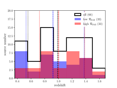
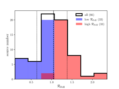
Figure 1: The relative Fe ii intensity and the redshift distributions of 66 MgII QSOs. Left panel: The FeiisubscriptFeii{\cal R}_{\rm{Fe\textsc{ii}}} distribution for the whole sample (black histogram), low-FeiisubscriptFeii{\cal R}_{\rm{Fe\textsc{ii}}} subsample (blue histogram), and the high-FeiisubscriptFeii{\cal R}_{\rm{Fe\textsc{ii}}} subsample (pink histogram). The dashed vertical line denotes the median FeiisubscriptFeii{\cal R}_{\rm{Fe\textsc{ii}}} value (1.0467), while the dotted vertical lines stand for the 16% and 84% percentile values (0.64 and 1.38, respectively). The bin size of the histogram is set by the Sturges’ and the Doane’s choice, ΔΔ\DeltaFeiisubscriptFeii{\cal R}_{\rm{Fe\textsc{ii}}}0.32similar-to-or-equalsabsent0.32\simeq 0.32, which both give 7 bins for the FeiisubscriptFeii{\cal R}_{\rm{Fe\textsc{ii}}}  range of (0.1,2.36)0.12.36(0.1,2.36). Right panel: The redshift distribution of 66 QSOs for the whole sample (black solid line), and low- and high-FeiisubscriptFeii{\cal R}_{\rm{Fe\textsc{ii}}} subsamples (33 sources in each subsample) that are depicted by blue and pink bars, respectively. The dashed vertical lines (black, blue, and red) stand for the corresponding median values for the whole, low-FeiisubscriptFeii{\cal R}_{\rm{Fe\textsc{ii}}}  and high-FeiisubscriptFeii{\cal R}_{\rm{Fe\textsc{ii}}} subsamples, respectively. The two sets of dotted vertical lines stand for the corresponding 16%- and 84%-percentiles for each sample. The bin size of the histogram is detemined via the Sturges’s and the Doane’s choice, Δz0.19similar-to-or-equalsΔ𝑧0.19\Delta z\simeq 0.19, which both yield 7 bins in the redshift range of (0.36,1.686)0.361.686(0.36,1.686).

3 Data

In this paper, we use 66 QSOs, with reverberation-measured time-delays of the broad Mg ii line with respect to the 3000Å  continuum, and with measurements of the intensity of the UV Fe ii pseudocontinuum given in terms of the ratio parameter FeiisubscriptFeii{\cal R}_{\rm{Fe\textsc{ii}}} =F(Feii22502650Å)/F(Mgii)absent𝐹Fesubscriptii22502650italic-Å𝐹Mgii=F(\mathrm{Fe}\textsc{ii}_{2250-2650\AA})/F(\mathrm{Mg}\textsc{ii}). These data are listed in Table LABEL:tab:MgQSOdata, including their redshifts, 3000Å  continuum flux densities, rest-frame time-delays of the MgII line, the UV FeiisubscriptFeii{\cal R}_{\rm{Fe\textsc{ii}}} parameter, and the original publication reference.

This Mg ii dataset spans the redshift range of 0.36z1.6860.36𝑧1.6860.36\leq z\leq 1.686 and is a subset of our earlier 78 Mg ii QSO compilation (Khadka et al., 2021b) for which the FeiisubscriptFeii{\cal R}_{\rm{Fe\textsc{ii}}} parameter is reliably inferred. The FeiisubscriptFeii{\cal R}_{\rm{Fe\textsc{ii}}} range for the whole sample is (0.1,2.36)0.12.36(0.1,2.36), or (1.0,0.37)1.00.37(-1.0,0.37) when using the log-scale. We also consider two low- and high-FeiisubscriptFeii{\cal R}_{\rm{Fe\textsc{ii}}} subsets of these 66 QSOs, divided at the median FeiisubscriptFeii{\cal R}_{\rm{Fe\textsc{ii}}} = 1.0467 value, each containing 33 QSOs. The FeiisubscriptFeii{\cal R}_{\rm{Fe\textsc{ii}}} distribution for 66 QSOs is shown in Fig. 1 (left panel), including the median as well as 16%- and 84%-percentile values of the distribution. The FeiisubscriptFeii{\cal R}_{\rm{Fe\textsc{ii}}}-subsample flag is included in Table LABEL:tab:MgQSOdata in the last column where (1) denotes a low-FeiisubscriptFeii{\cal R}_{\rm{Fe\textsc{ii}}} source and (2) corresponds to a high-FeiisubscriptFeii{\cal R}_{\rm{Fe\textsc{ii}}} source. The low-FeiisubscriptFeii{\cal R}_{\rm{Fe\textsc{ii}}} subset spans the redshift range 0.36z1.5870.36𝑧1.5870.36\leq z\leq 1.587 and the high-FeiisubscriptFeii{\cal R}_{\rm{Fe\textsc{ii}}} subset spans 0.4253z1.6860.4253𝑧1.6860.4253\leq z\leq 1.686. The redshift distribution of all 66 QSOs, as well as low- and high-FeiisubscriptFeii{\cal R}_{\rm{Fe\textsc{ii}}} subsamples, is displayed in Fig. 1 (right panel). For all the sources, the median redshift value is z=0.990𝑧0.990z=0.990 (0.556 and 1.384 for 16%- and 84% percentiles, respectively), while it is z=0.921𝑧0.921z=0.921 for low-FeiisubscriptFeii{\cal R}_{\rm{Fe\textsc{ii}}} (16% percentile: 0.527; 84% percentile: 1.376) and z=1.004𝑧1.004z=1.004 for high-FeiisubscriptFeii{\cal R}_{\rm{Fe\textsc{ii}}} sources (16% percentile: 0.723; 84% percentile: 1.384). The redshift distribution of the Mg ii QSOs is quite different from that of the Hβ𝛽\beta QSOs, which peaks at the lowest-redshift bin between z=0𝑧0z=0 and 0.10.10.1 for the whole Hβ𝛽\beta dataset as well as for low- and high-FeiisubscriptFeii{\cal R}_{\rm{Fe\textsc{ii}}} subsamples, see Fig. 1 in Khadka et al. (2021a).
Refer to caption
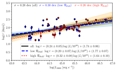
Figure 2: The Mg ii-based RL𝑅𝐿R-L relation ( in a spatially flat ΛΛ\LambdaCDM model with H0=70kms1Mpc1subscript𝐻070kmsuperscripts1superscriptMpc1H_{0}=70\,{\rm km\,s^{-1}\,Mpc^{-1}}, Ωm0=0.3subscriptΩ𝑚00.3\Omega_{m0}=0.3, and ΩΛ=0.7subscriptΩΛ0.7\Omega_{\Lambda}=0.7) for 66 QSOs with the inferred relative Fe ii intensities. The low-FeiisubscriptFeii{\cal R}_{\rm{Fe\textsc{ii}}} sources are depicted with blue circles, while high-FeiisubscriptFeii{\cal R}_{\rm{Fe\textsc{ii}}} sources are represented by red circles. The black solid, blue dashed, and red dotted lines correspond to the best-fit RL𝑅𝐿R-L relations for the whole sample, the low-, and the high-FeiisubscriptFeii{\cal R}_{\rm{Fe\textsc{ii}}} subsamples, respectively. The best-fit parameters are listed in the legend. The shaded areas around each line correspond to 1σ1𝜎1\sigma confidence intervals. The intrinsic rms scatter for each sample is listed along the top part of the plot.

The Mg ii RL𝑅𝐿R-L relation shows a significant positive correlation for the whole dataset of 66 sources as well as for the low-FeiisubscriptFeii{\cal R}_{\rm{Fe\textsc{ii}}} and the high-FeiisubscriptFeii{\cal R}_{\rm{Fe\textsc{ii}}} subsamples (33 sources in each subsample), see Fig. 2 for the graphical depiction of the RL𝑅𝐿R-L relation including the corresponding best-fit relations for all three datasets and the intrinsic scatters. For Fig. 2, to obtain the monochromatic luminosity at 300030003000 Å, we assume a spatially-flat ΛCDMΛCDM\Lambda\text{CDM} model with H0=70kms1Mpc1subscript𝐻070kmsuperscripts1superscriptMpc1H_{0}=70\,{\rm km\,s^{-1}\,Mpc^{-1}}, Ωm0=0.3subscriptΩ𝑚00.3\Omega_{m0}=0.3, and ΩΛ=0.7subscriptΩΛ0.7\Omega_{\Lambda}=0.7. It is clear that the best-fit RL𝑅𝐿R-L relations are consistent with each other within 1σ𝜎\sigma confidence intervals,

All:logτAll:𝜏\displaystyle\text{All:}\log{\tau} =(0.24±0.05)logL44+(1.74±0.06),absentplus-or-minus0.240.05subscript𝐿44plus-or-minus1.740.06\displaystyle=(0.24\pm 0.05)\log{L_{44}}+(1.74\pm 0.06)\,\,,
Low-Feii:logτLow-Feii:𝜏\displaystyle\text{Low-${\cal R}_{\rm{Fe\textsc{ii}}}$:}\log{\tau} =(0.20±0.07)logL44+(1.77±0.07),absentplus-or-minus0.200.07subscript𝐿44plus-or-minus1.770.07\displaystyle=(0.20\pm 0.07)\log{L_{44}}+(1.77\pm 0.07)\,\,,
High-Feii:logτHigh-Feii:𝜏\displaystyle\text{High-${\cal R}_{\rm{Fe\textsc{ii}}}$:}\log{\tau} =(0.32±0.08)logL44+(1.64±0.10),absentplus-or-minus0.320.08subscript𝐿44plus-or-minus1.640.10\displaystyle=(0.32\pm 0.08)\log{L_{44}}+(1.64\pm 0.10)\,\,, (13)

where τ𝜏\tau is the source-frame time delay expressed in days, L44=L3000/1044ergs1subscript𝐿44subscript𝐿3000superscript1044ergsuperscripts1L_{44}=L_{3000}/10^{44}\,{\rm erg\,s^{-1}} corresponds to the monochromatic 3000 Å luminosity L3000subscript𝐿3000L_{3000} (expressed in ergs1ergsuperscripts1{\rm erg\,s^{-1}}) normalized to 1044ergs1superscript1044ergsuperscripts110^{44}\,{\rm erg\,s^{-1}}, and loglog10subscript10\log\equiv\log_{10}. The intrinsic scatter of σext=0.28subscript𝜎ext0.28\sigma_{\rm ext}=0.28, 0.300.300.30, and 0.260.260.26 dex for the whole, low-FeiisubscriptFeii{\cal R}_{\rm{Fe\textsc{ii}}}, and high-FeiisubscriptFeii{\cal R}_{\rm{Fe\textsc{ii}}} samples are comparable, though it appears to be lower for the high-FeiisubscriptFeii{\cal R}_{\rm{Fe\textsc{ii}}} subsample. For the whole sample of 66 sources, the Pearson correlation coefficient is r=0.51𝑟0.51r=0.51 (p=1.01×10⁵𝑝1.01superscript105p=1.01\times 10^{-5}) and the Spearman rank-order correlation coefficient is s=0.40𝑠0.40s=0.40 (p=9.67×10⁴𝑝9.67superscript104p=9.67\times 10^{-4}). For the low-FeiisubscriptFeii{\cal R}_{\rm{Fe\textsc{ii}}} subsample, we obtain a Pearson correlation coefficient of r=0.46𝑟0.46r=0.46 (p=0.00738𝑝0.00738p=0.00738) and a Spearman rank-order correlation coefficient of s=0.37𝑠0.37s=0.37 (p=0.0354𝑝0.0354p=0.0354). For the high-FeiisubscriptFeii{\cal R}_{\rm{Fe\textsc{ii}}} subsample, the Pearson correlation coefficient is r=0.57𝑟0.57r=0.57 (p=5.79×10⁴𝑝5.79superscript104p=5.79\times 10^{-4}) and the Spearman rank-order correlation coefficient is s=0.48𝑠0.48s=0.48 (p=4.91×10³𝑝4.91superscript103p=4.91\times 10^{-3}). Hence, for the high-FeiisubscriptFeii{\cal R}_{\rm{Fe\textsc{ii}}} subsample the correlation is stronger and more significant than for the low-FeiisubscriptFeii{\cal R}_{\rm{Fe\textsc{ii}}} subsample.

Refer to caption
Refer to caption
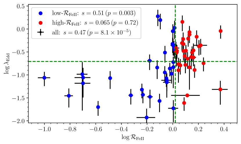
Figure 3: Relation between the relative Fe ii strength expressed by the ratio FeiisubscriptFeii{\cal R}_{\rm{Fe\textsc{ii}}}  and the Eddington ratio λEddsubscript𝜆Edd\lambda_{\rm Edd} (top panel) and the dimensionless accretion rate ˙˙\dot{\mathcal{M}} (bottom panel). The dashed green lines mark the median values of the corresponding quantities. For the whole sample, FeiisubscriptFeii{\cal R}_{\rm{Fe\textsc{ii}}}  shows a significant positive correlation with respect to both quantities as measured by the Spearman correlation coefficient, see the legend. However, when the sample is divided the significance of the correlation drops considerably, especially for the high-FeiisubscriptFeii{\cal R}_{\rm{Fe\textsc{ii}}} subsample, which exhibits no significant correlation with the quantities of interest.

The main motivation for including the FeiisubscriptFeii{\cal R}_{\rm{Fe\textsc{ii}}} parameter is that it is expected to be correlated with the Eddington ratio λEddsubscript𝜆Edd\lambda_{\rm Edd}888The Eddington ratio is λEddLbol/LEddsubscript𝜆Eddsubscript𝐿bolsubscript𝐿Edd\lambda_{\rm Edd}\equiv L_{\rm bol}/L_{\rm Edd}, where Lbolsubscript𝐿bolL_{\rm bol} is the bolometric luminosity calculated as Lbol=κbolL3000subscript𝐿bolsubscript𝜅bolsubscript𝐿3000L_{\rm bol}=\kappa_{\rm bol}L_{3000}, where κbolsubscript𝜅bol\kappa_{\rm bol} is the bolometric correction factor taken from Netzer (2019). LEddsubscript𝐿EddL_{\rm Edd} stands for the Eddington luminosity, where we adopt the standard relation for stationary spherical accretion. The black hole mass is calculated using the reveberation method, M=fvircτFWHM2/Gsubscript𝑀subscript𝑓vir𝑐𝜏superscriptFWHM2𝐺M_{\bullet}=f_{\rm vir}c\tau\text{FWHM}^{2}/G, where FWHM is the full width at half maximum in kms1kmsuperscripts1{\rm km\,s^{-1}} for the Mg ii line, and fvirsubscript𝑓virf_{\rm vir} is the virial factor calculated using the FWHM-dependent relation for Mg ii (Mejía-Restrepo et al., 2018). or the dimensionless accretion-rate ˙˙\dot{\mathcal{M}} (Panda et al., 2019c; Śniegowska et al., 2020). 999The dimensionless accretion rate is ˙=26.2(L44/cosθ)3/2m72˙26.2superscriptsubscript𝐿44𝜃32superscriptsubscript𝑚72\dot{\mathcal{M}}=26.2(L_{44}/\cos{\theta})^{3/2}m_{7}^{-2} (Wang et al., 2014), where θ𝜃\theta is the accretion-disk angle with respect to the line of sight and we fix cosθ=0.75𝜃0.75\cos{\theta}=0.75 according to the mean angle for type I AGN taking into account the covering factor of the dusty molecular torus (Lawrence & Elvis, 2010; Ichikawa et al., 2015). m7subscript𝑚7m_{7} is the reverberation-measured black hole mass scaled to 107Msuperscript107subscript𝑀direct-product10^{7}\,M_{\odot}, i.e. m7M/(107M)subscript𝑚7subscript𝑀superscript107subscript𝑀direct-productm_{7}\equiv M_{\bullet}/(10^{7}\,M_{\odot}). Since both λEddsubscript𝜆Edd\lambda_{\rm Edd} and ˙˙\dot{\mathcal{M}} depend on the Mg ii QSO black-hole mass that is determined via reverberation mapping, they are intrinsically correlated with τ𝜏\tau as well as L3000subscript𝐿3000L_{3000}. Their inclusion would bias the extended RL𝑅𝐿R-L relation, which is avoided by using the independent observable FeiisubscriptFeii{\cal R}_{\rm{Fe\textsc{ii}}}. Since the scatter about the RL𝑅𝐿R-L relation appears to be driven by the accretion rate (Martínez-Aldama et al., 2020b), the inclusion of FeiisubscriptFeii{\cal R}_{\rm{Fe\textsc{ii}}} as an independent observable could in principle decrease the scatter. We show the correlation between FeiisubscriptFeii{\cal R}_{\rm{Fe\textsc{ii}}} and the two accretion-rate quantities in Fig. 3, computed in the fixed flat ΛΛ\LambdaCDM model of the previous paragraph. For the whole sample of 66 sources, FeiisubscriptFeii{\cal R}_{\rm{Fe\textsc{ii}}} exhibits a significant positive correlation with both λEddsubscript𝜆Edd\lambda_{\rm Edd} and ˙˙\dot{\mathcal{M}} as measured by the Spearman rank-order correlation coefficient, s=0.47𝑠0.47s=0.47 (p=8.07×10⁵𝑝8.07superscript105p=8.07\times 10^{-5}) and s=0.46𝑠0.46s=0.46 (p=9.77×10⁵𝑝9.77superscript105p=9.77\times 10^{-5}), respectively. However, when the sample is divided in two with respect to the median of FeiisubscriptFeii{\cal R}_{\rm{Fe\textsc{ii}}}, the correlation significance drops considerably, especially for the high-FeiisubscriptFeii{\cal R}_{\rm{Fe\textsc{ii}}} subsample, which does not show a significant correlation.

In this study, we also use 11 BAO measurements listed in Table 1 of Khadka & Ratra (2021) and 31 H(z)𝐻𝑧H(z) observations listed in Table 2 of Ryan et al. (2018). We use the better-established joint BAO+H(z)𝐻𝑧H(z) sample cosmological constraints for comparison with the cosmological constraints based on Mg ii QSOs, in all 6 cosmological models considered in this study.

4 Methods and Model comparison

First, we consider the 2-parameter RL𝑅𝐿R-L relation using eq. (4) with k=0𝑘0k=0; see also Khadka et al. (2021b) for the analysis using 78 Mg ii  QSOs and the 2-parameter RL𝑅𝐿R-L relation. When we analyse Mg ii data assuming the 2-parameter RL𝑅𝐿R-L relation, we denote the three data sets without a prime (Mg ii QSO-66, Mg ii low-FeiisubscriptFeii{\cal R}_{\rm{Fe\textsc{ii}}}, and Mg ii high-FeiisubscriptFeii{\cal R}_{\rm{Fe\textsc{ii}}}).

Attempts have been made to correct for the accretion rate effect observed in the 2-parameter RL𝑅𝐿R-L relation (Du & Wang, 2019; Martínez-Aldama et al., 2020b; Zajaček et al., 2021) by extending it to a 3-parameter RL𝑅𝐿R-L relation; the hope is that this will reduce the intrinsic dispersion and result in tighter cosmological constraints. In our Hβ𝛽\beta QSO work (Khadka et al., 2021a) we did not find evidence for this, however, the Hβ𝛽\beta QSO cosmological constraints were somewhat inconsistent with those from better-established cosmological probes. Here we examine this issue for Mg ii QSOs whose cosmological constraints are consistent with those from better-established cosmological probes (Khadka et al., 2021b).

For this study we consider two 3-parameter RL𝑅𝐿R-L relations, the first being eq. (4) with q=𝑞absentq=FeiisubscriptFeii{\cal R}_{\rm{Fe\textsc{ii}}}  where k𝑘k is the third free parameter associated with the intensity of the UV Fe ii  flux ratio parameter FeiisubscriptFeii{\cal R}_{\rm{Fe\textsc{ii}}} and must be determined from data. When we analyse Mg ii data assuming this 3-parameter RL𝑅𝐿R-L relation we denote the three data sets with a single prime (Mg ii QSO-66, Mg ii low-FeiisubscriptFeii{\cal R}_{\rm{Fe\textsc{ii}}}, and Mg ii high-FeiisubscriptFeii{\cal R}_{\rm{Fe\textsc{ii}}}).

The second 3-parameter RL𝑅𝐿R-L relation we use assumes a power-law dependency of τ𝜏\tau on FeiisubscriptFeii{\cal R}_{\rm{Fe\textsc{ii}}}  hence q=log𝑞q=\logFeiisubscriptFeii{\cal R}_{\rm{Fe\textsc{ii}}}  in eq. (4). When we analyse Mg ii data assuming this 3-parameter RL𝑅𝐿R-L relation we denote the three data sets with a double prime (Mg ii′′ QSO-66, Mg ii′′ low-FeiisubscriptFeii{\cal R}_{\rm{Fe\textsc{ii}}}, and Mg ii′′ high-FeiisubscriptFeii{\cal R}_{\rm{Fe\textsc{ii}}}).

The rest-frame time-delay of a QSO at known redshift in a given cosmological model can be theoretically predicted using eq. (4), along with eqs. (1) and (2). The log likelihood function that compares predicted time-delays with the corresponding observed time-delays, and so allows us to determine the constraints on cosmological-model and QSO-correlation parameters, is (D’Agostini, 2005)

ln(LF)=12i=1N[[log(τX,iobs)log(τX,ith)]2si2+ln(2πsi2)].LF12subscriptsuperscript𝑁𝑖1delimited-[]superscriptdelimited-[]subscriptsuperscript𝜏obs𝑋𝑖subscriptsuperscript𝜏th𝑋𝑖2subscriptsuperscript𝑠2𝑖2𝜋subscriptsuperscript𝑠2𝑖\ln({\rm LF})=-\frac{1}{2}\sum^{N}_{i=1}\left[\frac{[\log(\tau^{\rm obs}_{X,i})-\log(\tau^{\rm th}_{X,i})]^{2}}{s^{2}_{i}}+\ln(2\pi s^{2}_{i})\right]. (14)

Here ln\ln = logesubscript𝑒\log_{e}, τX,ith(p)subscriptsuperscript𝜏th𝑋𝑖p\tau^{\rm th}_{X,i}(\textbf{\emph{p}}) and τX,iobssubscriptsuperscript𝜏obs𝑋𝑖\tau^{\rm obs}_{X,i} are the predicted and observed time-delays at measured redshift zisubscript𝑧𝑖z_{i}. In the 2-parameter RL𝑅𝐿R-L relation case, si2=σlogτobs,i2+γ2σlogF3000,i2+σext2subscriptsuperscript𝑠2𝑖subscriptsuperscript𝜎2subscript𝜏obs𝑖superscript𝛾2subscriptsuperscript𝜎2subscript𝐹3000𝑖superscriptsubscript𝜎ext2s^{2}_{i}=\sigma^{2}_{\log{\tau_{\rm obs},i}}+\gamma^{2}\sigma^{2}_{\log{F_{3000},i}}+\sigma_{\rm ext}^{2}, while in the linear 3-parameter RL𝑅𝐿R-L relation case, si2=σlogτobs,i2+γ2σlogF3000,i2+k2σFeII,i2+σext2subscriptsuperscript𝑠2𝑖subscriptsuperscript𝜎2subscript𝜏obs𝑖superscript𝛾2subscriptsuperscript𝜎2subscript𝐹3000𝑖superscript𝑘2subscriptsuperscript𝜎2subscriptFeII𝑖superscriptsubscript𝜎ext2s^{2}_{i}=\sigma^{2}_{\log{\tau_{\rm obs},i}}+\gamma^{2}\sigma^{2}_{\log{F_{3000},i}}+k^{2}\sigma^{2}_{{\cal R}_{\text{Fe{\sc II}}},i}+\sigma_{\rm ext}^{2}, where σlogτobs,isubscript𝜎subscript𝜏obs𝑖\sigma_{\log{\tau_{\rm obs},i}}, σlogF3000,isubscript𝜎subscript𝐹3000𝑖\sigma_{\log{F_{3000},i}}, and σFeII,isubscript𝜎subscriptFeII𝑖\sigma_{{\cal R}_{\text{Fe{\sc II}}},i} are the measurement errors on the observed time-delay (τX,iobssubscriptsuperscript𝜏obs𝑋𝑖\tau^{\rm obs}_{X,i}), measured flux (F3000,isubscript𝐹3000𝑖F_{3000,i}), and measured FeiisubscriptFeii{\cal R}_{\rm{Fe\textsc{ii}}},i respectively, and in the log 3-parameter RL𝑅𝐿R-L relation case, si2=σlogτobs,i2+γ2σlogF3000,i2+k2σlogFeII,i2+σext2subscriptsuperscript𝑠2𝑖subscriptsuperscript𝜎2subscript𝜏obs𝑖superscript𝛾2subscriptsuperscript𝜎2subscript𝐹3000𝑖superscript𝑘2subscriptsuperscript𝜎2subscriptFeII𝑖superscriptsubscript𝜎ext2s^{2}_{i}=\sigma^{2}_{\log{\tau_{\rm obs},i}}+\gamma^{2}\sigma^{2}_{\log{F_{3000},i}}+k^{2}\sigma^{2}_{\log{{\cal R}_{\text{Fe{\sc II}}}},i}+\sigma_{\rm ext}^{2}, where σlogFeII,isubscript𝜎subscriptFeII𝑖\sigma_{\log{{\cal R}_{\text{Fe{\sc II}}}},i} is the measurement error on the measured log FeiisubscriptFeii{\cal R}_{\rm{Fe\textsc{ii}}},i. σextsubscript𝜎ext\sigma_{\rm ext} is the intrinsic dispersion of the RL𝑅𝐿R-L relation.

The BAO + H(z)𝐻𝑧H(z) cosmological constraints used here are from Khadka & Ratra (2021); see that paper for the derivation and description of these constraints. The better-established BAO+H(z)𝐻𝑧H(z) data cosmological constraints are used for comparison with the Mg ii QSO cosmological constraints.

We perform Markov chain Monte Carlo (MCMC) sampling, as implemented in the MontePython code (Brinckmann & Lesgourgues, 2019), to maximize the log likelihood function given in eq. (14). We use top hat priors for each free parameter, see Table 1. Mg ii data cannot constrain H0subscript𝐻0H_{0} because of the degeneracy between β𝛽\beta and H0subscript𝐻0H_{0}, so in QSO data analyses we set H0subscript𝐻0H_{0} to 707070 kms1Mpc1kmsuperscripts1superscriptMpc1{\rm km}\hskip 2.84526pt{\rm s}^{-1}{\rm Mpc}^{-1}. Each MCMC chain satisfies the Gelman-Rubin convergence criterion, R1<0.05𝑅10.05R-1<0.05. The MCMC sampling chains are analysed using the Python package Getdist (Lewis, 2019).

Table 1: Non-zero flat prior parameter ranges.
Parameter Prior range
Ωbh2subscriptΩ𝑏superscript2\Omega_{b}h^{2} [0,1]01[0,1]
Ωch2subscriptΩ𝑐superscript2\Omega_{c}h^{2} [0,1]01[0,1]
Ωm0subscriptΩ𝑚0\Omega_{m0} [0,1]01[0,1]
Ωk0subscriptΩ𝑘0\Omega_{k0} [2,2]22[-2,2]
ωXsubscript𝜔𝑋\omega_{X} [5,0.33]50.33[-5,0.33]
α𝛼\alpha [0,10]010[0,10]
σextsubscript𝜎ext\sigma_{\rm ext} [0,5]05[0,5]
β𝛽\beta [0,10]010[0,10]
γ𝛾\gamma [0,5]05[0,5]
k𝑘k [10,10]1010[-10,10]

We compute the Akaike and the Bayesian information criterion (AIC𝐴𝐼𝐶AIC and BIC𝐵𝐼𝐶BIC) values and use them for the comparison of different RL𝑅𝐿R-L relations. These are

AIC=𝐴𝐼𝐶absent\displaystyle AIC= 2ln(LFmax)+2d,2subscriptLFmax2𝑑\displaystyle-2\ln({\rm LF}_{\rm max})+2d, (15)
BIC=𝐵𝐼𝐶absent\displaystyle BIC= 2ln(LFmax)+dlnN,2subscriptLFmax𝑑𝑁\displaystyle-2\ln({\rm LF}_{\rm max})+d\ln{N}\,, (16)

where LFmaxsubscriptLFmax\rm LF_{\rm max} is the maximum likelihood value, d𝑑d is the number of free parameters, and N𝑁N is the number of data points, with the degrees of freedom dof=Nd𝑑𝑜𝑓𝑁𝑑dof=N-d. We compute ΔAICΔ𝐴𝐼𝐶\Delta AIC and ΔBICΔ𝐵𝐼𝐶\Delta BIC differences of the 3-parameter RL𝑅𝐿R-L relations with respect to the corresponding 2-parameter RL𝑅𝐿R-L reference model. Positive (negative) values of ΔAICΔ𝐴𝐼𝐶\Delta AIC or ΔBICΔ𝐵𝐼𝐶\Delta BIC indicate that the 3-parameter correlation relation under investigation fit the measurements worse (better) than the 2-parameter reference one. ΔAIC(BIC)[0,2]Δ𝐴𝐼𝐶𝐵𝐼𝐶02\Delta AIC(BIC)\in[0,2] is weak evidence in favor of the 2-parameter reference relation, ΔAIC(BIC)(2,6]Δ𝐴𝐼𝐶𝐵𝐼𝐶26\Delta AIC(BIC)\in(2,6] is positive evidence for the reference relation, ΔAIC(BIC)>6Δ𝐴𝐼𝐶𝐵𝐼𝐶6\Delta AIC(BIC)>6 is strong evidence for the reference relation, and ΔAIC(BIC)>10Δ𝐴𝐼𝐶𝐵𝐼𝐶10\Delta AIC(BIC)>10 is very strong evidence for the reference reference.

5 Results

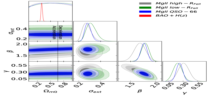
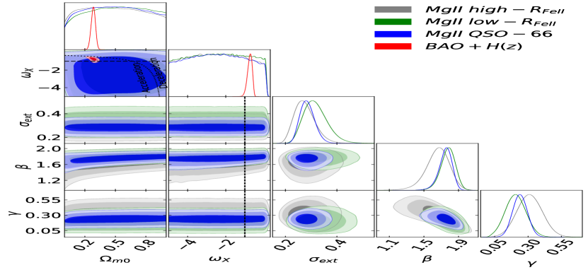
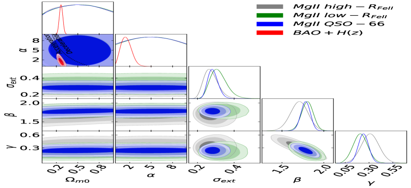
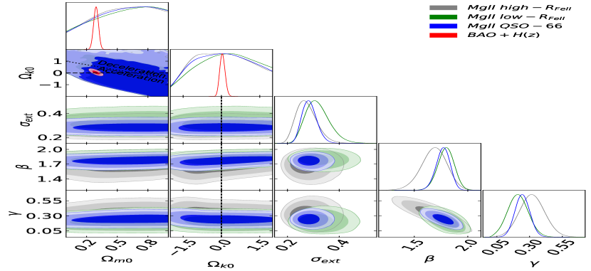
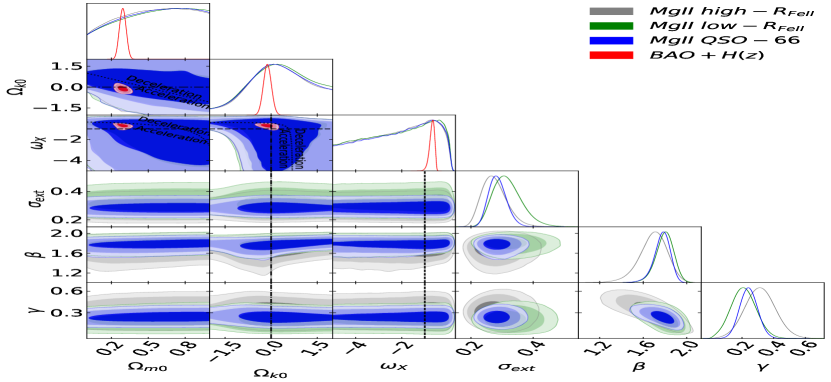
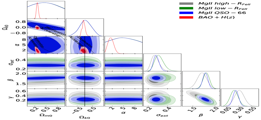
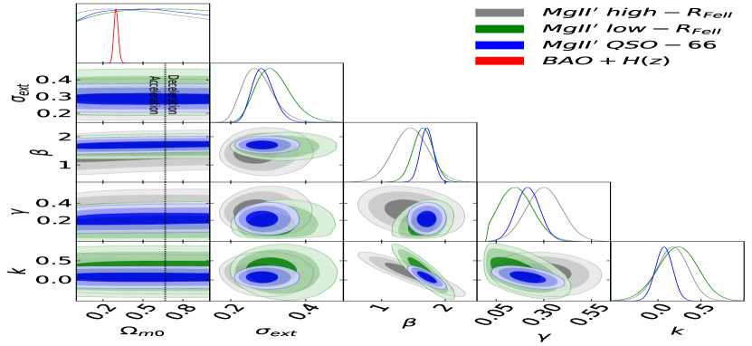
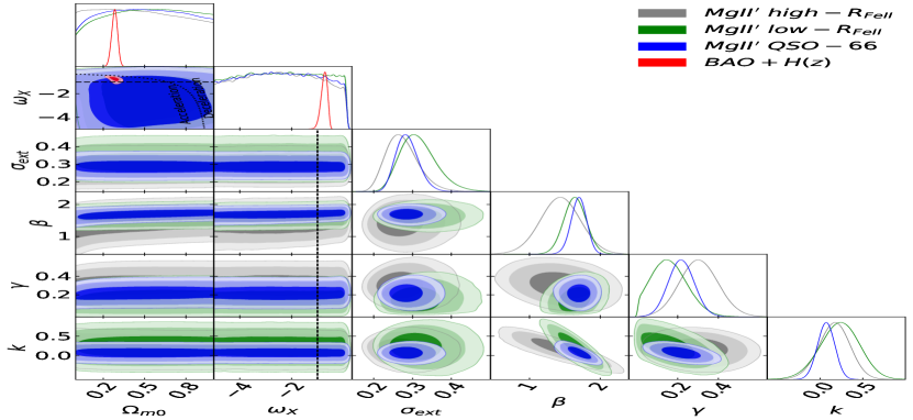
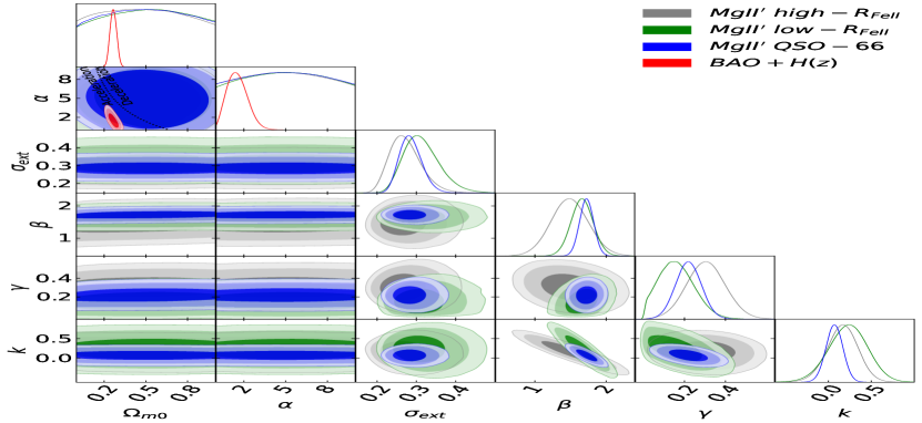
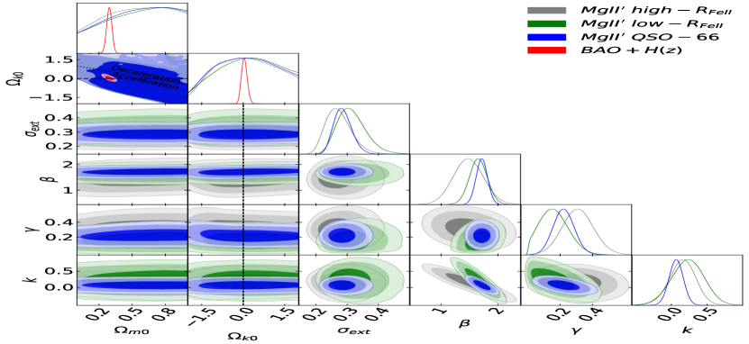
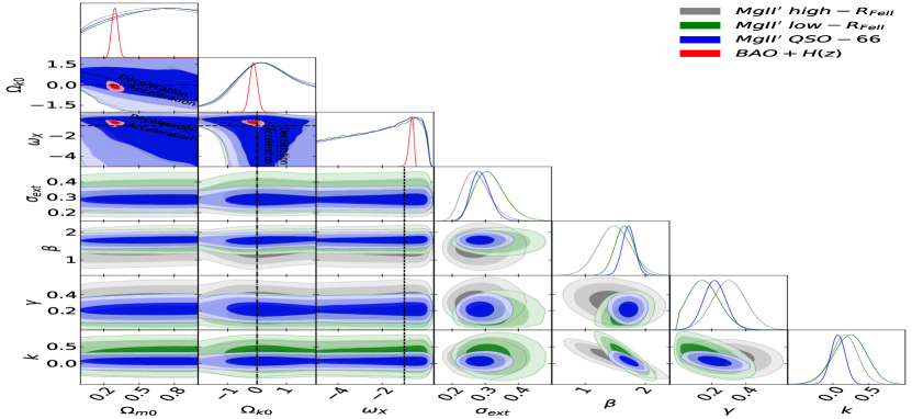
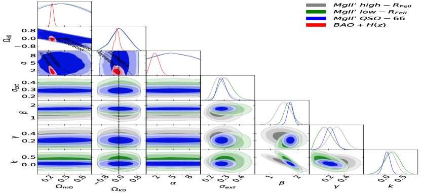
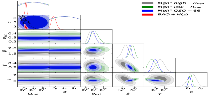
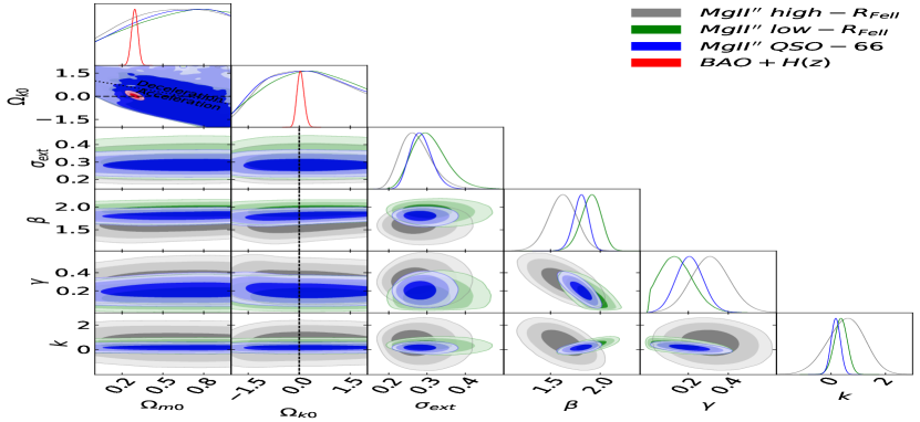
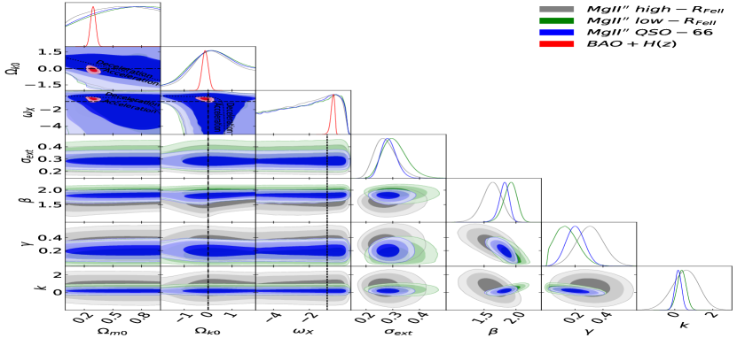
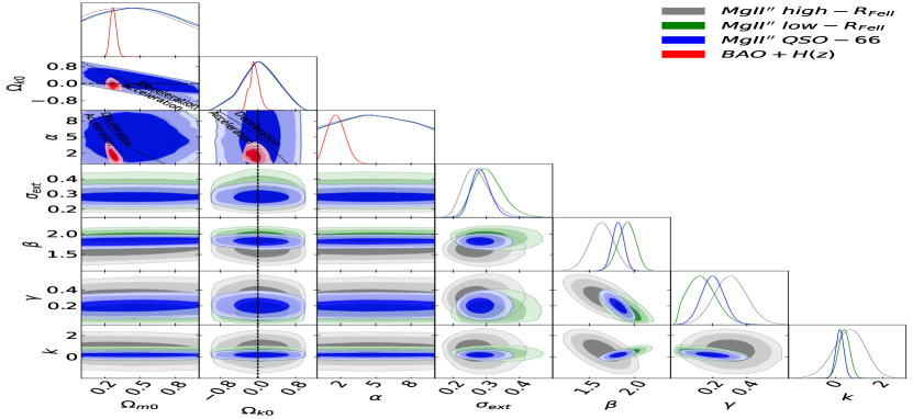
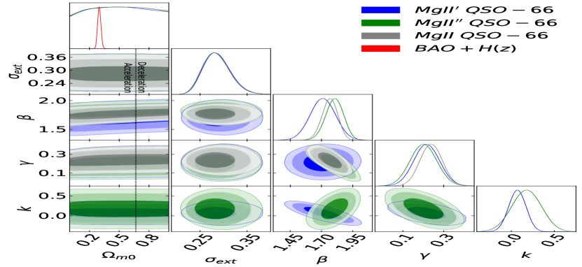
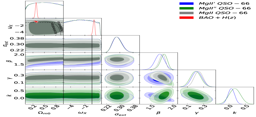
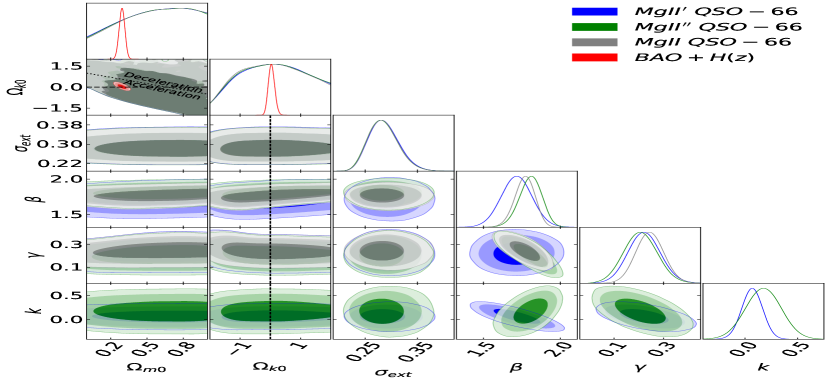
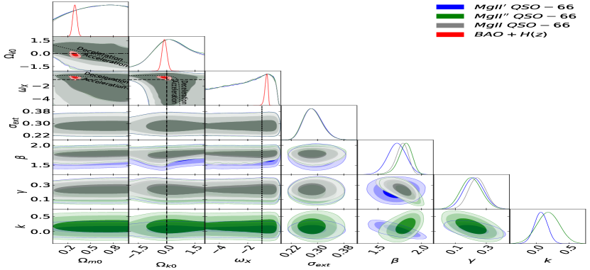
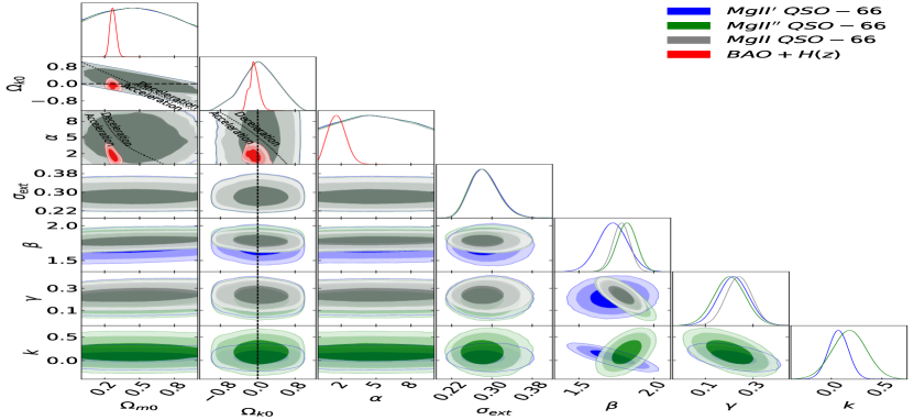
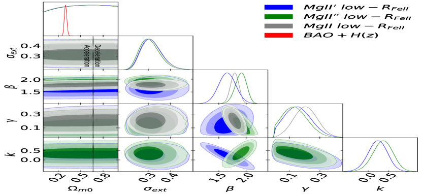
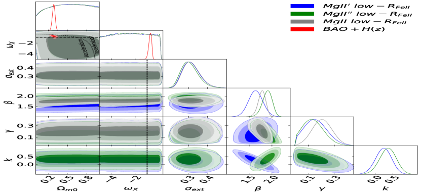
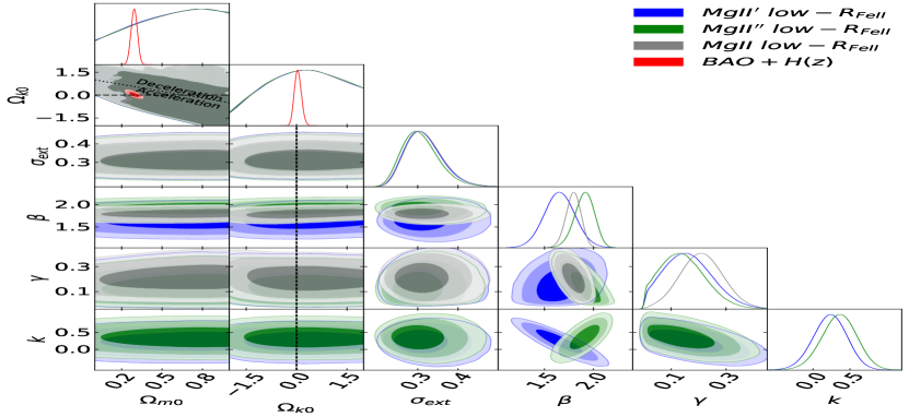
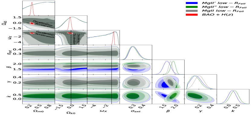
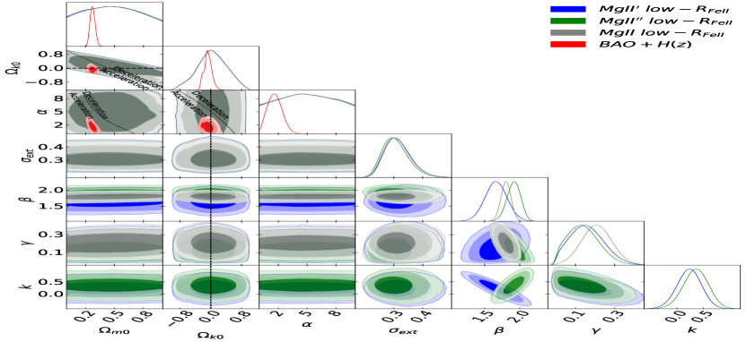
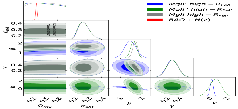
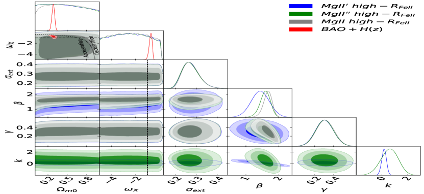
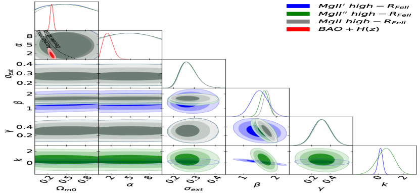
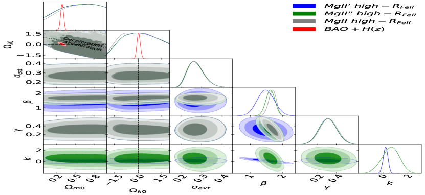
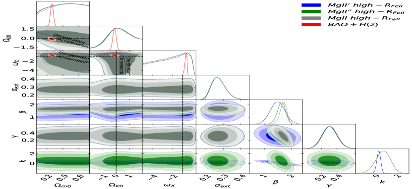
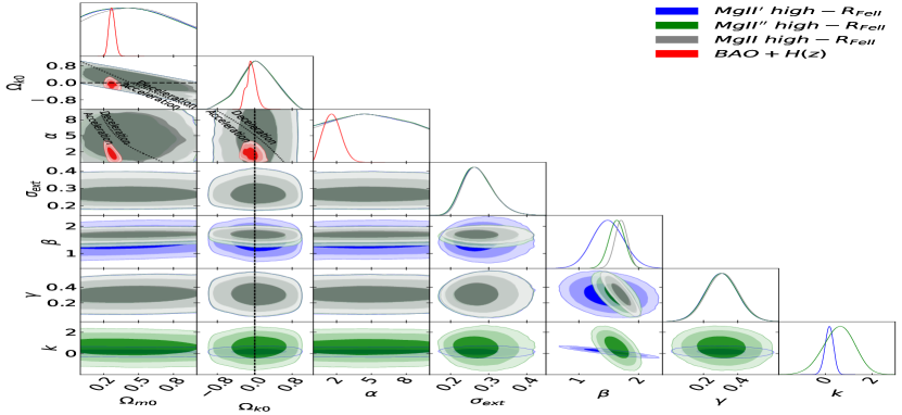
Results from the analyses of the QSO and BAO + H(z)𝐻𝑧H(z) data sets are listed in Tables LABEL:tab:1 and LABEL:tab:2. Unmarginalized best-fit parameter values are given in Table LABEL:tab:1 and marginalized best-fit parameter values and error bars are listed in Table LABEL:tab:2. One-dimensional likelihoods and two-dimensional likelihood contours are shown in Figs. 49.

We use the BAO + H(z)𝐻𝑧H(z) results to compare with the results from the QSO data sets. This comparison allows us to draw a qualitative conclusion about the consistency or inconsistency between the QSO results and the results from other well-established cosmological data. From Figs. 49 we see that the Mg ii QSO cosmological constraints are consistent with those derived from BAO + H(z)𝐻𝑧H(z) data, which is also the case for the cosmological constraints derived from the full 78 source Mg ii data set (Khadka et al., 2021b). This, however, differs from what happens with the Hβ𝛽\beta sources whose cosmological constraints are 2σsimilar-toabsent2𝜎\sim 2\sigma inconsistent with the BAO + H(z)𝐻𝑧H(z) cosmological constraints (Khadka et al., 2021a).

From Table LABEL:tab:2, for the 2-parameter Mg ii QSO-66 data set, in all models, the measured values of β𝛽\beta, γ𝛾\gamma, and σextsubscript𝜎ext\sigma_{\rm ext} lie in the range 1.7470.061+0.086subscriptsuperscript1.7470.0860.0611.747^{+0.086}_{-0.061} to 1.7820.056+0.056subscriptsuperscript1.7820.0560.0561.782^{+0.056}_{-0.056}, 0.2390.055+0.055subscriptsuperscript0.2390.0550.0550.239^{+0.055}_{-0.055} to 0.2450.057+0.057subscriptsuperscript0.2450.0570.0570.245^{+0.057}_{-0.057}, and 0.2850.032+0.024subscriptsuperscript0.2850.0240.0320.285^{+0.024}_{-0.032} to 0.2860.032+0.024subscriptsuperscript0.2860.0240.0320.286^{+0.024}_{-0.032} respectively. For the 3-parameter linear-FeiisubscriptFeii{\cal R}_{\rm{Fe\textsc{ii}}} Mg ii QSO-66 data set, in all models, the measured values of β𝛽\beta, γ𝛾\gamma, k𝑘k, and σextsubscript𝜎ext\sigma_{\rm ext} lie in the range 1.6900.110+0.110subscriptsuperscript1.6900.1100.1101.690^{+0.110}_{-0.110} to 1.7250.098+0.098subscriptsuperscript1.7250.0980.0981.725^{+0.098}_{-0.098}, 0.2170.063+0.063subscriptsuperscript0.2170.0630.0630.217^{+0.063}_{-0.063} to 0.2230.066+0.066subscriptsuperscript0.2230.0660.0660.223^{+0.066}_{-0.066}, 0.0690.099+0.099subscriptsuperscript0.0690.0990.0990.069^{+0.099}_{-0.099} to 0.0700.100+0.100subscriptsuperscript0.0700.1000.1000.070^{+0.100}_{-0.100}, and 0.2860.032+0.024subscriptsuperscript0.2860.0240.0320.286^{+0.024}_{-0.032} to 0.2870.032+0.025subscriptsuperscript0.2870.0250.0320.287^{+0.025}_{-0.032} respectively. For the 3-parameter log-FeiisubscriptFeii{\cal R}_{\rm{Fe\textsc{ii}}} Mg ii′′ QSO-66 data set, in all models, the measured values of β𝛽\beta, γ𝛾\gamma, k𝑘k, and σextsubscript𝜎ext\sigma_{\rm ext} lie in the range 1.7870.070+0.091subscriptsuperscript1.7870.0910.0701.787^{+0.091}_{-0.070} to 1.8180.065+0.065subscriptsuperscript1.8180.0650.0651.818^{+0.065}_{-0.065}, 0.2010.065+0.065subscriptsuperscript0.2010.0650.0650.201^{+0.065}_{-0.065} to 0.2070.068+0.068subscriptsuperscript0.2070.0680.0680.207^{+0.068}_{-0.068}, 0.1700.170+0.170subscriptsuperscript0.1700.1700.1700.170^{+0.170}_{-0.170} to 0.1800.170+0.170subscriptsuperscript0.1800.1700.1700.180^{+0.170}_{-0.170}, and 0.2840.032+0.024subscriptsuperscript0.2840.0240.0320.284^{+0.024}_{-0.032} to 0.2860.032+0.024subscriptsuperscript0.2860.0240.0320.286^{+0.024}_{-0.032} respectively. In each of the three QSO-66 data sets the RL𝑅𝐿R-L correlation parameter values are independent, within the error bars, of the cosmological model used in the analysis and so all three QSO-66 data sets are standardizable.101010This is also true for all the high-FeiisubscriptFeii{\cal R}_{\rm{Fe\textsc{ii}}} and low-FeiisubscriptFeii{\cal R}_{\rm{Fe\textsc{ii}}} data subsets. Importantly, there is no change in the intrinsic dispersion σextsubscript𝜎ext\sigma_{\rm ext} when going from the 2-parameter RL𝑅𝐿R-L relation to either of the 3-parameter RL𝑅𝐿R-L relations. This differs mildly from what happens in the Hβ𝛽\beta case (Khadka et al., 2021a) where σextsubscript𝜎ext\sigma_{\rm ext} is about 0.75σ𝜎\sigma smaller in the 3-parameter linear-FeiisubscriptFeii{\cal R}_{\rm{Fe\textsc{ii}}} RL𝑅𝐿R-L relation case compared to the 2-parameter one.111111Khadka et al. (2021a) did not study the log-FeiisubscriptFeii{\cal R}_{\rm{Fe\textsc{ii}}} 3-parameter relation in the Hβ𝛽\beta case.

From Table LABEL:tab:2, for the 2-parameter Mg ii low-FeiisubscriptFeii{\cal R}_{\rm{Fe\textsc{ii}}} data subset, in all models, the measured values of β𝛽\beta, γ𝛾\gamma, and σextsubscript𝜎ext\sigma_{\rm ext} lie in the range 1.7760.074+0.092subscriptsuperscript1.7760.0920.0741.776^{+0.092}_{-0.074} to 1.8030.072+0.072subscriptsuperscript1.8030.0720.0721.803^{+0.072}_{-0.072}, 0.2070.078+0.078subscriptsuperscript0.2070.0780.0780.207^{+0.078}_{-0.078} to 0.2120.079+0.079subscriptsuperscript0.2120.0790.0790.212^{+0.079}_{-0.079}, and 0.3160.054+0.038subscriptsuperscript0.3160.0380.0540.316^{+0.038}_{-0.054} to 0.3180.053+0.036subscriptsuperscript0.3180.0360.0530.318^{+0.036}_{-0.053} respectively. For the 2-parameter Mg ii high-FeiisubscriptFeii{\cal R}_{\rm{Fe\textsc{ii}}} data subset, in all models, the measured values of β𝛽\beta, γ𝛾\gamma, and σextsubscript𝜎ext\sigma_{\rm ext} lie in the range 1.6600.110+0.150subscriptsuperscript1.6600.1500.1101.660^{+0.150}_{-0.110} to 1.7100.110+0.110subscriptsuperscript1.7100.1100.1101.710^{+0.110}_{-0.110}, 0.3100.095+0.095subscriptsuperscript0.3100.0950.0950.310^{+0.095}_{-0.095} to 0.3200.098+0.098subscriptsuperscript0.3200.0980.0980.320^{+0.098}_{-0.098}, and 0.2750.046+0.031subscriptsuperscript0.2750.0310.0460.275^{+0.031}_{-0.046} to 0.2760.047+0.031subscriptsuperscript0.2760.0310.0470.276^{+0.031}_{-0.047} respectively. From Table 4, for the 2-parameter Mg ii low-FeiisubscriptFeii{\cal R}_{\rm{Fe\textsc{ii}}} and high-FeiisubscriptFeii{\cal R}_{\rm{Fe\textsc{ii}}} data subsets, the difference in β𝛽\beta values, ΔβΔ𝛽\Delta\beta, between different cosmological models lie in the range (0.64–0.77)σ𝜎\sigma which is not statistically significant. The difference in γ𝛾\gamma values, ΔγΔ𝛾\Delta\gamma, between different cosmological models lie in the range (0.84–0.86)σ𝜎\sigma which is not statistically significant. The difference in σextsubscript𝜎ext\sigma_{\rm ext} values, ΔσextΔsubscript𝜎ext\Delta\sigma_{\rm ext} between different cosmological models lie in the range (0.65–0.69)σ𝜎\sigma which is statistically insignificant. This is very different from what happens with the 2-parameter RL𝑅𝐿R-L relation for Hβ𝛽\beta QSOs where Δβ(34)σsimilar-toΔ𝛽34𝜎\Delta\beta\sim(3-4)\sigma (Khadka et al., 2021a).

From Table LABEL:tab:2, for the 3-parameter linear-FeiisubscriptFeii{\cal R}_{\rm{Fe\textsc{ii}}} Mg ii low-FeiisubscriptFeii{\cal R}_{\rm{Fe\textsc{ii}}} data subset, in all models, the measured values of β𝛽\beta, γ𝛾\gamma, k𝑘k, and σextsubscript𝜎ext\sigma_{\rm ext} lie in the range 1.6400.160+0.160subscriptsuperscript1.6400.1600.1601.640^{+0.160}_{-0.160} to 1.6600.160+0.160subscriptsuperscript1.6600.1600.1601.660^{+0.160}_{-0.160}, 0.1620.100+0.072subscriptsuperscript0.1620.0720.1000.162^{+0.072}_{-0.100} to 0.1650.100+0.073subscriptsuperscript0.1650.0730.1000.165^{+0.073}_{-0.100}, 0.2300.230+0.230subscriptsuperscript0.2300.2300.2300.230^{+0.230}_{-0.230}, and 0.3150.053+0.036subscriptsuperscript0.3150.0360.0530.315^{+0.036}_{-0.053} to 0.3160.054+0.036subscriptsuperscript0.3160.0360.0540.316^{+0.036}_{-0.054} respectively. For the 3-parameter linear-FeiisubscriptFeii{\cal R}_{\rm{Fe\textsc{ii}}} Mg ii high-FeiisubscriptFeii{\cal R}_{\rm{Fe\textsc{ii}}} data subset, in all models, the measured values of β𝛽\beta, γ𝛾\gamma, k𝑘k, and σextsubscript𝜎ext\sigma_{\rm ext} lie in the range 1.4300.290+0.290subscriptsuperscript1.4300.2900.2901.430^{+0.290}_{-0.290} to 1.4900.270+0.270subscriptsuperscript1.4900.2700.2701.490^{+0.270}_{-0.270}, 0.3050.098+0.098subscriptsuperscript0.3050.0980.0980.305^{+0.098}_{-0.098} to 0.3110.098+0.098subscriptsuperscript0.3110.0980.0980.311^{+0.098}_{-0.098}, 0.1500.190+0.190subscriptsuperscript0.1500.1900.1900.150^{+0.190}_{-0.190} to 0.1600.190+0.190subscriptsuperscript0.1600.1900.1900.160^{+0.190}_{-0.190}, and 0.2730.047+0.031subscriptsuperscript0.2730.0310.0470.273^{+0.031}_{-0.047} to 0.2750.047+0.032subscriptsuperscript0.2750.0320.0470.275^{+0.032}_{-0.047} respectively. From Table 5, for the 3-parameter linear-FeiisubscriptFeii{\cal R}_{\rm{Fe\textsc{ii}}} Mg ii low-FeiisubscriptFeii{\cal R}_{\rm{Fe\textsc{ii}}} and high-FeiisubscriptFeii{\cal R}_{\rm{Fe\textsc{ii}}} data subsets, the difference in β𝛽\beta values, ΔβΔ𝛽\Delta\beta, between different cosmological models lie in the range (0.54–0.63)σ𝜎\sigma which is statistically insignificant. The difference in γ𝛾\gamma values, ΔγΔ𝛾\Delta\gamma, between different cosmological models lie in the range (1.17–1.19)σ𝜎\sigma which is not statistically significant. The difference in k𝑘k values, ΔkΔ𝑘\Delta k, between different cosmological models lie in the range (0.23–0.27)σ𝜎\sigma which is statistically insignificant. The difference in σextsubscript𝜎ext\sigma_{\rm ext} values, ΔσextΔsubscript𝜎ext\Delta\sigma_{\rm ext}, between different cosmological models lie in the range (0.65–0.69)σ𝜎\sigma which is statistically insignificant. Mostly these differences are insignificant but ΔγΔ𝛾\Delta\gamma are larger than in the 2-parameter RL𝑅𝐿R-L relation case shown in Table 4. This differs from what happens with the Hβ𝛽\beta sources, where ΔγΔ𝛾\Delta\gamma are smaller in the 3-parameter case compared to the 2-parameter case (Khadka et al., 2021a).

From Table LABEL:tab:2, for the 3-parameter log-FeiisubscriptFeii{\cal R}_{\rm{Fe\textsc{ii}}} Mg ii′′ low-FeiisubscriptFeii{\cal R}_{\rm{Fe\textsc{ii}}} data subset, in all models, the measured values of β𝛽\beta, γ𝛾\gamma, k𝑘k, and σextsubscript𝜎ext\sigma_{\rm ext} lie in the range 1.8900.094+0.120subscriptsuperscript1.8900.1200.0941.890^{+0.120}_{-0.094} to 1.9100.092+0.110subscriptsuperscript1.9100.1100.0921.910^{+0.110}_{-0.092}, 0.1420.097+0.063subscriptsuperscript0.1420.0630.0970.142^{+0.063}_{-0.097} to 0.1460.098+0.064subscriptsuperscript0.1460.0640.0980.146^{+0.064}_{-0.098}, 0.3500.240+0.240subscriptsuperscript0.3500.2400.2400.350^{+0.240}_{-0.240} to 0.3600.240+0.240subscriptsuperscript0.3600.2400.2400.360^{+0.240}_{-0.240}, and 0.3070.051+0.035subscriptsuperscript0.3070.0350.0510.307^{+0.035}_{-0.051} to 0.3090.053+0.035subscriptsuperscript0.3090.0350.0530.309^{+0.035}_{-0.053} respectively. For the 3-parameter log-FeiisubscriptFeii{\cal R}_{\rm{Fe\textsc{ii}}} Mg ii′′ high-FeiisubscriptFeii{\cal R}_{\rm{Fe\textsc{ii}}} data subset, in all models, the measured values of β𝛽\beta, γ𝛾\gamma, k𝑘k, and σextsubscript𝜎ext\sigma_{\rm ext} lie in the range 1.5800.140+0.170subscriptsuperscript1.5800.1700.1401.580^{+0.170}_{-0.140} to 1.6400.130+0.130subscriptsuperscript1.6400.1300.1301.640^{+0.130}_{-0.130}, 0.3040.095+0.095subscriptsuperscript0.3040.0950.0950.304^{+0.095}_{-0.095} to 0.3120.098+0.098subscriptsuperscript0.3120.0980.0980.312^{+0.098}_{-0.098}, 0.5500.650+0.730subscriptsuperscript0.5500.7300.6500.550^{+0.730}_{-0.650} to 0.5900.650+0.720subscriptsuperscript0.5900.7200.6500.590^{+0.720}_{-0.650}, and 0.2720.047+0.032subscriptsuperscript0.2720.0320.0470.272^{+0.032}_{-0.047} to 0.2750.048+0.033subscriptsuperscript0.2750.0330.0480.275^{+0.033}_{-0.048} respectively. From Table 6, for the 3-parameter log-FeiisubscriptFeii{\cal R}_{\rm{Fe\textsc{ii}}} Mg ii′′ low-FeiisubscriptFeii{\cal R}_{\rm{Fe\textsc{ii}}} and high-FeiisubscriptFeii{\cal R}_{\rm{Fe\textsc{ii}}} data subsets, the difference in β𝛽\beta values, ΔβΔ𝛽\Delta\beta, between different cosmological models lie in the range (1.58–1.78)σ𝜎\sigma which could be statistically significant. The difference in γ𝛾\gamma values, ΔγΔ𝛾\Delta\gamma, between different cosmological models lie in the range (1.40–1.44)σ𝜎\sigma which could be statistically significant. The difference in k𝑘k values, ΔkΔ𝑘\Delta k, between different cosmological models lie in the range (0.27–0.35)σ𝜎\sigma which is statistically insignificant. The difference in σextsubscript𝜎ext\sigma_{\rm ext} values, ΔσextΔsubscript𝜎ext\Delta\sigma_{\rm ext}, between different cosmological models lie in the range (0.54–0.58)σ𝜎\sigma which is statistically insignificant. ΔβΔ𝛽\Delta\beta values are (somewhat significantly) larger in the log-FeiisubscriptFeii{\cal R}_{\rm{Fe\textsc{ii}}} 3-parameter case compared to the linear-FeiisubscriptFeii{\cal R}_{\rm{Fe\textsc{ii}}} 3-parameter and the 2-parameter RL𝑅𝐿R-L correlation cases shown in Tables 5 and 4.

This difference in ΔβΔ𝛽\Delta\beta values is connected to the smaller and mostly negative range of log FeiisubscriptFeii{\cal R}_{\rm{Fe\textsc{ii}}} (1.0,0.37)1.00.37(-1.0,0.37) in comparison to the larger and positive range of FeiisubscriptFeii{\cal R}_{\rm{Fe\textsc{ii}}} (0.1,2.36)0.12.36(0.1,2.36). This results in the normalization, β𝛽\beta, values being larger in the log-FeiisubscriptFeii{\cal R}_{\rm{Fe\textsc{ii}}} case compared to those in the linear-FeiisubscriptFeii{\cal R}_{\rm{Fe\textsc{ii}}} case. Another qualitative difference is that Mg ii′′ high-FeiisubscriptFeii{\cal R}_{\rm{Fe\textsc{ii}}} sources always have positive log FeiisubscriptFeii{\cal R}_{\rm{Fe\textsc{ii}}} values, with mean value of 0.130.130.13, while Mg ii′′ low-FeiisubscriptFeii{\cal R}_{\rm{Fe\textsc{ii}}} sources have mostly negative log FeiisubscriptFeii{\cal R}_{\rm{Fe\textsc{ii}}} values, with mean value of 0.210.21-0.21. This apparently makes the inferred high- and low-FeiisubscriptFeii{\cal R}_{\rm{Fe\textsc{ii}}} β𝛽\beta values differ more in the log-FeiisubscriptFeii{\cal R}_{\rm{Fe\textsc{ii}}} case than in the linear-FeiisubscriptFeii{\cal R}_{\rm{Fe\textsc{ii}}} case.

From Table LABEL:tab:1, from the ΔAICΔ𝐴𝐼𝐶\Delta AIC values, there is mostly only weak evidence (mostly) for or against the 2-parameter RL𝑅𝐿R-L relation. The exceptions for the 66 source data set are the flat ΛΛ\LambdaCDM model and the non-flat XCDM parametrization where there is positive evidence for and against the 2-parameter RL𝑅𝐿R-L relation relative to the 3-parameter linear-FeiisubscriptFeii{\cal R}_{\rm{Fe\textsc{ii}}} RL𝑅𝐿R-L relations, respectively. From the ΔBICΔ𝐵𝐼𝐶\Delta BIC values, in all 66 source cases, there is positive evidence in favor of the 2-parameter RL𝑅𝐿R-L relation over the 3-parameter RL𝑅𝐿R-L relations. The high- and low-FeiisubscriptFeii{\cal R}_{\rm{Fe\textsc{ii}}} data subset ΔBICΔ𝐵𝐼𝐶\Delta BIC values indicate that the 2-parameter relation is weakly or positively favored over both the 3-parameter relations. The results for the 66 source data set analyses are dramatically different from those for the full Hβ𝛽\beta data set analyses (Khadka et al., 2021a) where the linear-FeiisubscriptFeii{\cal R}_{\rm{Fe\textsc{ii}}} 3-parameter RL𝑅𝐿R-L is very strongly favored over the 2-parameter one. This difference is a consequence of the significant difference between low- and high-FeiisubscriptFeii{\cal R}_{\rm{Fe\textsc{ii}}} Hβ𝛽\beta sources relative to the small difference between these two subsets in the Mg ii case here.

When considering the full Mg ii sample, using both the linear- and log-FeiisubscriptFeii{\cal R}_{\rm{Fe\textsc{ii}}} relations, k𝑘k is consistent with zero at less than 1σ1𝜎1\sigma. It is only for the Mg ii′′ low-FeiisubscriptFeii{\cal R}_{\rm{Fe\textsc{ii}}} case that k𝑘k is a little less than 1.5σ𝜎\sigma away from zero. This is another indication that FeiisubscriptFeii{\cal R}_{\rm{Fe\textsc{ii}}} is of no significant relevance for current Mg ii  data. This is another difference compared to the Hβ𝛽\beta case, where k<0𝑘0k<0 at more than 4σ𝜎\sigma for the full sample in the linear-FeiisubscriptFeii{\cal R}_{\rm{Fe\textsc{ii}}} case.

The Mg ii cosmological constraints obtained in this paper are listed in Table LABEL:tab:2. They are weak. Since we have found no reason to favor either of the 3-parameter RL𝑅𝐿R-L relations over the 2-parameter one, the 2-parameter RL𝑅𝐿R-L relation cosmological constraints derived in Khadka et al. (2021b) from the complete 78 source data set are the appropriate Mg ii cosmological constraints.

Table 2: Unmarginalized best-fit parameters for all data sets.
Model Data set Ωbh2subscriptΩ𝑏superscript2\Omega_{b}h^{2} Ωch2subscriptΩ𝑐superscript2\Omega_{c}h^{2} Ωm0subscriptΩ𝑚0\Omega_{m0} Ωk0subscriptΩ𝑘0\Omega_{k0} ωXsubscript𝜔𝑋\omega_{X} α𝛼\alpha H0subscript𝐻0H_{0}a σextsubscript𝜎ext\sigma_{\rm ext} β𝛽\beta γ𝛾\gamma k𝑘k dof𝑑𝑜𝑓dof 2ln(LFmax)2subscriptLFmax-2\ln({\rm LF}_{\rm max}) AIC𝐴𝐼𝐶AIC BIC𝐵𝐼𝐶BIC ΔAICΔ𝐴𝐼𝐶\Delta AIC ΔBICΔ𝐵𝐼𝐶\Delta BIC
Mg ii QSO-66 - - 0.211 - - - - 0.274 1.745 0.230 - 62 20.52 28.52 37.28 - -
Flat Mg ii low-FeiisubscriptFeii{\cal R}_{\rm{Fe\textsc{ii}}} - - 0.534 - - - - 0.291 1.796 0.206 - 29 14.30 22.30 28.29 - -
ΛΛ\LambdaCDM Mg ii high-FeiisubscriptFeii{\cal R}_{\rm{Fe\textsc{ii}}} - - 0.132 - - - - 0.253 1.651 0.294 - 29 4.64 12.64 18.63 - -
Mg ii QSO-66 - - 0.120 - - - - 0.272 1.684 0.202 0.076 61 19.90 29.90 40.85 1.381.381.38 3.573.573.57
Mg ii low-FeiisubscriptFeii{\cal R}_{\rm{Fe\textsc{ii}}} - - 0.993 - - - - 0.284 1.662 0.149 0.255 28 12.90 22.90 30.38 0.600.600.60 2.092.092.09
Mg ii high-FeiisubscriptFeii{\cal R}_{\rm{Fe\textsc{ii}}} - - 0.027 - - - - 0.243 1.375 0.278 0.194 28 3.12 13.12 20.60 0.480.480.48 1.971.971.97
Mg ii′′ QSO-66 - - 0.088 - - - - 0.270 1.817 0.270 0.182 61 19.26 26.29 40.21 -2.23 2.932.932.93
Mg ii′′ low-FeiisubscriptFeii{\cal R}_{\rm{Fe\textsc{ii}}} - - 0.959 - - - - 0.276 1.939 0.122 0.393 28 11.34 21.34 28.82 -0.96 0.530.530.53
Mg ii′′ high-FeiisubscriptFeii{\cal R}_{\rm{Fe\textsc{ii}}} - - 0.030 - - - - 0.241 1.546 0.272 0.791 28 3.10 13.10 20.58 0.460.460.46 1.951.951.95
BAO + H(z)𝐻𝑧H(z) 0.024 0.119 0.298 - - - 69.119 - - - - 39 23.66 29.66 34.87 - -
Mg ii QSO-66 - - 0.347 1.0501.050-1.050 - - - 0.271 1.683 0.295 - 61 18.28 28.28 39.23 - -
Non-flat Mg ii low-FeiisubscriptFeii{\cal R}_{\rm{Fe\textsc{ii}}} - - 0.393 -1.120 - - - 0.286 1.731 0.237 - 28 14.08 24.08 31.56 - -
ΛΛ\LambdaCDM Mg ii high-FeiisubscriptFeii{\cal R}_{\rm{Fe\textsc{ii}}} - - 0.254 -0.853 - - - 0.242 1.561 0.368 - 28 1.22 11.22 18.70 - -
Mg ii QSO-66 - - 0.337 -1.025 - - - 0.272 1.645 0.253 0.057 60 18.16 30.16 43.30 1.881.881.88 4.074.074.07
Mg ii low-FeiisubscriptFeii{\cal R}_{\rm{Fe\textsc{ii}}} - - 0.737 -1.773 - - - 0.281 1.632 0.195 0.230 27 12.78 24.78 33.76 0.700.700.70 2.202.202.20
Mg ii high-FeiisubscriptFeii{\cal R}_{\rm{Fe\textsc{ii}}} - - 0.237 -0.800 - - - 0.239 1.392 0.392 0.094 27 0.84 12.84 21.82 1.621.621.62 3.123.123.12
Mg ii′′ QSO-66 - - 0.291 -0.933 - - - 0.271 1.722 0.251 0.108 60 17.56 29.56 42.70 1.281.281.28 3.473.473.47
Mg ii′′ low-FeiisubscriptFeii{\cal R}_{\rm{Fe\textsc{ii}}} - - 0.615 -1.587 - - - 0.280 1.883 0.164 0.367 27 11.22 23.22 32.20 -0.86 0.640.640.64
Mg ii′′ high-FeiisubscriptFeii{\cal R}_{\rm{Fe\textsc{ii}}} - - 0.214 -0.750 - - - 0.230 1.525 0.343 0.426 27 0.90 12.90 21.88 1.681.681.68 3.183.183.18
BAO + H(z)𝐻𝑧H(z) 0.025 0.114 0.294 0.021 - - 68.701 - - - - 38 23.60 31.60 38.55 - -
Mg ii QSO-66 - - 0.002 - -4.549 - - 0.276 1.517 0.178 - 61 19.58 29.58 40.53 - -
Flat Mg ii low-FeiisubscriptFeii{\cal R}_{\rm{Fe\textsc{ii}}} - - 0.431 - 1.4541.454-1.454 - - 0.291 1.780 0.205 - 28 14.30 24.30 31.78 - -
XCDM Mg ii high-FeiisubscriptFeii{\cal R}_{\rm{Fe\textsc{ii}}} - - 0.000 - 4.9104.910-4.910 - - 0.233 1.287 0.234 - 28 2.46 12.46 19.94 - -
Mg ii QSO-66 - - 0.015 - -3.639 - - 0.265 1.520 0.178 0.094 60 18.96 30.96 44.10 1.381.381.38 3.573.573.57
Mg ii low-FeiisubscriptFeii{\cal R}_{\rm{Fe\textsc{ii}}} - - 0.280 - 0.091 - - 0.285 1.656 0.143 0.272 27 12.90 24.90 33.88 0.600.600.60 2.102.102.10
Mg ii high-FeiisubscriptFeii{\cal R}_{\rm{Fe\textsc{ii}}} - - 0.002 - -4.373 - - 0.223 0.980 0.228 0.297 27 0.40 12.40 21.38 -0.06 1.441.441.44
Mg ii′′ QSO-66 - - 0.003 - -4.524 - - 0.268 1.559 0.170 0.151 60 18.34 30.34 43.48 0.760.760.76 2.952.952.95
Mg ii′′ low-FeiisubscriptFeii{\cal R}_{\rm{Fe\textsc{ii}}} - - 0.770 - 0.058 - - 0.276 1.939 0.128 0.375 27 11.34 23.34 32.32 -0.96 0.540.540.54
Mg ii′′ high-FeiisubscriptFeii{\cal R}_{\rm{Fe\textsc{ii}}} - - 0.002 - -4.655 - - 0.244 1.102 0.274 1.136 27 0.120.12-0.12 11.88 20.86 -0.58 0.920.920.92
BAO + H(z)𝐻𝑧H(z) 0.031 0.088 0.280 - -0.691 - 65.036 - - - - 38 19.66 27.66 34.61 - -
Mg ii QSO-66 - - 0.129 -0.248 -2.424 - - 0.264 1.552 0.261 - 60 16.38 28.38 41.52 - -
Non-flat Mg ii low-FeiisubscriptFeii{\cal R}_{\rm{Fe\textsc{ii}}} - - 0.154 -0.353 -1.771 - - 0.293 1.697 0.187 - 27 13.88 25.88 34.86 - -
XCDM Mg ii high-FeiisubscriptFeii{\cal R}_{\rm{Fe\textsc{ii}}} - - 0.073 0.1520.152-0.152 -2.501 - - 0.213 1.298 0.372 - 27 -3.34 8.66 17.64 - -
Mg ii QSO-66 - - 0.110 -0.231 -2.246 - - 0.260 1.565 0.268 0.0040.004-0.004 59 15.96 29.96 45.29 1.581.581.58 3.773.773.77
Mg ii low-FeiisubscriptFeii{\cal R}_{\rm{Fe\textsc{ii}}} - - 0.634 -1.833 -0.776 - - 0.285 1.628 0.167 0.261 26 12.78 26.78 37.26 0.900.900.90 2.402.402.40
Mg ii high-FeiisubscriptFeii{\cal R}_{\rm{Fe\textsc{ii}}} - - 0.054 -0.133 -2.083 - - 0.213 1.163 0.316 0.167 26 2.562.56-2.56 11.44 21.92 2.782.782.78 4.284.284.28
Mg ii′′ QSO-66 - - 0.146 -0.326 -1.886 - - 0.282 1.620 0.254 0.065 59 16.42 30.42 45.75 2.042.042.04 4.234.234.23
Mg ii′′ low-FeiisubscriptFeii{\cal R}_{\rm{Fe\textsc{ii}}} - - 0.991 -1.250 -4.657 - - 0.271 1.865 0.166 0.424 26 11.22 25.22 35.70 -0.66 0.840.840.84
Mg ii′′ high-FeiisubscriptFeii{\cal R}_{\rm{Fe\textsc{ii}}} - - 0.039 -0.084 -2.682 - - 0.215 1.248 0.377 0.164 26 5.285.28-5.28 8.72 19.20 0.060.060.06 1.561.561.56
BAO + H(z)𝐻𝑧H(z) 0.030 0.094 0.291 -0.147 -0.641 - 65.204 - - - - 37 18.34 28.34 37.03 - -
Mg ii QSO-66 - - 0.123 - - 0.174 - 0.273 1.739 0.229 - 61 20.56 30.56 41.51 - -
Flat Mg ii low-FeiisubscriptFeii{\cal R}_{\rm{Fe\textsc{ii}}} - - 0.866 - - 5.741 - 0.291 1.816 0.214 - 28 14.30 24.30 31.78 - -
ϕitalic-ϕ\phiCDM Mg II high-FeiisubscriptFeii{\cal R}_{\rm{Fe\textsc{ii}}} - - 0.096 - - 0.113 - 0.250 1.652 0.291 - 28 4.64 14.64 22.12 - -
Mg ii QSO-66 - - 0.143 - - 0.217 - 0.272 1.681 0.209 0.078 60 19.92 31.92 45.06 1.361.361.36 3.553.553.55
Mg ii low-FeiisubscriptFeii{\cal R}_{\rm{Fe\textsc{ii}}} - - 0.957 - - 0.814 - 0.281 1.660 0.150 0.262 27 12.90 24.90 33.88 0.600.600.60 2.102.102.10
Mg ii high-FeiisubscriptFeii{\cal R}_{\rm{Fe\textsc{ii}}} - - 0.039 - - 0.196 - 0.243 1.336 0.282 0.231 27 3.20 15.20 24.18 0.600.600.60 2.062.062.06
Mg ii′′ QSO-66 - - 0.197 - - 0.089 - 0.275 1.786 0.198 0.182 60 19.28 31.28 44.42 0.720.720.72 2.912.912.91
Mg ii′′ low-FeiisubscriptFeii{\cal R}_{\rm{Fe\textsc{ii}}} - - 0.969 - - 6.156 - 0.278 1.937 0.126 0.385 27 11.34 23.34 32.32 -0.96 0.540.540.54
Mg ii′′ high-FeiisubscriptFeii{\cal R}_{\rm{Fe\textsc{ii}}} - - 0.028 - - 0.397 - 0.238 1.564 0.271 0.776 27 3.20 15.20 24.18 0.560.560.56 2.062.062.06
BAO + H(z)𝐻𝑧H(z) 0.033 0.080 0.265 - - 1.445 65.272 - - - - 38 19.56 27.56 34.51 - -
Mg ii QSO-66 - - 0.342 -0.308 - 0.194 - 0.275 1.746 0.238 - 60 20.44 32.44 45.58 - -
Non-flat Mg ii low-FeiisubscriptFeii{\cal R}_{\rm{Fe\textsc{ii}}} - - 0.987 -0.854 - 0.393 - 0.291 1.809 0.210 - 27 14.28 26.28 35.26 - -
ϕitalic-ϕ\phiCDM Mg ii high-FeiisubscriptFeii{\cal R}_{\rm{Fe\textsc{ii}}} - - 0.278 -0.267 - 0.136 - 0.245 1.649 0.316 - 27 4.58 16.58 25.56 - -
Mg ii QSO-66 - - 0.487 -0.365 - 0.404 - 0.271 1.718 0.219 0.057 59 19.94 33.94 49.27 1.501.501.50 3.693.693.69
Mg ii low-FeiisubscriptFeii{\cal R}_{\rm{Fe\textsc{ii}}} - - 0.970 -0.898 - 5.136 - 0.282 1.672 0.154 0.255 26 12.88 26.88 37.36 0.600.600.60 2.102.102.10
Mg ii high-FeiisubscriptFeii{\cal R}_{\rm{Fe\textsc{ii}}} - - 0.064 0.042 - 0.082 - 0.243 1.431 0.298 0.155 26 3.32 17.32 27.80 0.740.740.74 2.242.242.24
Mg ii′′ QSO-66 - - 0.401 -0.191 - 0.331 - 0.268 1.804 0.202 0.188 59 19.24 33.24 48.57 0.800.800.80 2.992.992.99
Mg ii′′ low-FeiisubscriptFeii{\cal R}_{\rm{Fe\textsc{ii}}} - - 0.857 -0.708 - 3.576 - 0.280 1.942 0.124 0.384 26 11.32 25.32 35.80 -0.96 0.530.530.53
Mg ii′′ high-FeiisubscriptFeii{\cal R}_{\rm{Fe\textsc{ii}}} - - 0.065 -0.021 - 0.315 - 0.248 1.545 0.284 0.727 26 3.30 17.30 27.78 0.720.720.72 2.222.222.22
BAO + H(z)𝐻𝑧H(z) 0.035 0.078 0.261 -0.155 - 2.042 65.720 - - - - 37 18.16 28.16 36.85 - -

a kms1Mpc1kmsuperscripts1superscriptMpc1{\rm km}\hskip 2.84526pt{\rm s}^{-1}{\rm Mpc}^{-1}. H0subscript𝐻0H_{0} is set to 707070 kms1Mpc1kmsuperscripts1superscriptMpc1{\rm km}\hskip 2.84526pt{\rm s}^{-1}{\rm Mpc}^{-1} for the QSO-only analyses.
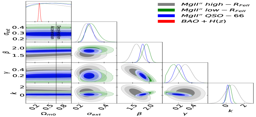
Table 3: Marginalized one-dimensional best-fit parameters with 1σ𝜎\sigma confidence intervals or 2σ𝜎\sigma limits for all data sets.
Model Data       Ωbh2subscriptΩ𝑏superscript2\Omega_{b}h^{2}       Ωch2subscriptΩ𝑐superscript2\Omega_{c}h^{2}       Ωm0subscriptΩ𝑚0\Omega_{m0}       ΩΛsubscriptΩΛ\Omega_{\Lambda}a       Ωk0subscriptΩ𝑘0\Omega_{k0}       ωXsubscript𝜔𝑋\omega_{X}       α𝛼\alpha       H0subscript𝐻0H_{0}b       σextsubscript𝜎ext\sigma_{\rm ext}       β𝛽\beta       γ𝛾\gamma       k𝑘k
Mg ii QSO-66 - - 0.4900.280+0.280subscriptsuperscript0.4900.2800.2800.490^{+0.280}_{-0.280} - - - - 0.2850.032+0.024subscriptsuperscript0.2850.0240.0320.285^{+0.024}_{-0.032} 1.7660.0620.062subscriptsuperscript1.7660.0620.0621.766^{-0.062}_{-0.062} 0.2390.055+0.055subscriptsuperscript0.2390.0550.0550.239^{+0.055}_{-0.055} -
Flat Mg ii low-FeiisubscriptFeii{\cal R}_{\rm{Fe\textsc{ii}}} - - 0.4900.480+0.260subscriptsuperscript0.4900.2600.4800.490^{+0.260}_{-0.480} - - - - 0.3180.054+0.036subscriptsuperscript0.3180.0360.0540.318^{+0.036}_{-0.054} 1.7900.0770.077subscriptsuperscript1.7900.0770.0771.790^{-0.077}_{-0.077} 0.2070.078+0.078subscriptsuperscript0.2070.0780.0780.207^{+0.078}_{-0.078} -
ΛΛ\LambdaCDM Mg ii high-FeiisubscriptFeii{\cal R}_{\rm{Fe\textsc{ii}}} - - 0.5000.310+0.360subscriptsuperscript0.5000.3600.3100.500^{+0.360}_{-0.310} - - - - 0.2760.047+0.031subscriptsuperscript0.2760.0310.0470.276^{+0.031}_{-0.047} 1.6800.1200.120subscriptsuperscript1.6800.1200.1201.680^{-0.120}_{-0.120} 0.3100.095+0.095subscriptsuperscript0.3100.0950.0950.310^{+0.095}_{-0.095} -
Mg ii QSO-66 - - 0.5000.280+0.280subscriptsuperscript0.5000.2800.2800.500^{+0.280}_{-0.280} - - - - 0.2870.032+0.025subscriptsuperscript0.2870.0250.0320.287^{+0.025}_{-0.032} 1.7100.1000.100subscriptsuperscript1.7100.1000.1001.710^{-0.100}_{-0.100} 0.2170.063+0.063subscriptsuperscript0.2170.0630.0630.217^{+0.063}_{-0.063} 0.0700.100+0.100subscriptsuperscript0.0700.1000.1000.070^{+0.100}_{-0.100}
Mg ii low-FeiisubscriptFeii{\cal R}_{\rm{Fe\textsc{ii}}} - - 0.4900.480+0.230subscriptsuperscript0.4900.2300.4800.490^{+0.230}_{-0.480} - - - - 0.3160.054+0.036subscriptsuperscript0.3160.0360.0540.316^{+0.036}_{-0.054} 1.6500.1600.160subscriptsuperscript1.6500.1600.1601.650^{-0.160}_{-0.160} 0.1620.100+0.072subscriptsuperscript0.1620.0720.1000.162^{+0.072}_{-0.100} 0.2300.240+0.240subscriptsuperscript0.2300.2400.2400.230^{+0.240}_{-0.240}
Mg ii high-FeiisubscriptFeii{\cal R}_{\rm{Fe\textsc{ii}}} - - 0.5200.230+0.470subscriptsuperscript0.5200.4700.2300.520^{+0.470}_{-0.230} - - - - 0.2740.048+0.032subscriptsuperscript0.2740.0320.0480.274^{+0.032}_{-0.048} 1.4600.2700.270subscriptsuperscript1.4600.2700.2701.460^{-0.270}_{-0.270} 0.3030.095+0.095subscriptsuperscript0.3030.0950.0950.303^{+0.095}_{-0.095} 0.1600.190+0.190subscriptsuperscript0.1600.1900.1900.160^{+0.190}_{-0.190}
Mg ii′′ QSO-66 - - 0.4900.280+0.280subscriptsuperscript0.4900.2800.2800.490^{+0.280}_{-0.280} - - - - 0.2850.032+0.025subscriptsuperscript0.2850.0250.0320.285^{+0.025}_{-0.032} 1.8040.071+0.071subscriptsuperscript1.8040.0710.0711.804^{+0.071}_{-0.071} 0.2010.065+0.065subscriptsuperscript0.2010.0650.0650.201^{+0.065}_{-0.065} 0.1800.170+0.170subscriptsuperscript0.1800.1700.1700.180^{+0.170}_{-0.170}
Mg ii′′ low-FeiisubscriptFeii{\cal R}_{\rm{Fe\textsc{ii}}} - - 0.4900.480+0.300subscriptsuperscript0.4900.3000.4800.490^{+0.300}_{-0.480} - - - - 0.3090.053+0.036subscriptsuperscript0.3090.0360.0530.309^{+0.036}_{-0.053} 1.9000.0940.110subscriptsuperscript1.9000.1100.0941.900^{-0.110}_{-0.094} 0.1430.097+0.064subscriptsuperscript0.1430.0640.0970.143^{+0.064}_{-0.097} 0.3500.240+0.240subscriptsuperscript0.3500.2400.2400.350^{+0.240}_{-0.240}
Mg ii′′ high-FeiisubscriptFeii{\cal R}_{\rm{Fe\textsc{ii}}} - - 0.5200.190+0.470subscriptsuperscript0.5200.4700.1900.520^{+0.470}_{-0.190} - - - - 0.2730.048+0.032subscriptsuperscript0.2730.0320.0480.273^{+0.032}_{-0.048} 1.6100.1400.140subscriptsuperscript1.6100.1400.1401.610^{-0.140}_{-0.140} 0.3040.095+0.095subscriptsuperscript0.3040.0950.0950.304^{+0.095}_{-0.095} 0.5900.650+0.720subscriptsuperscript0.5900.7200.6500.590^{+0.720}_{-0.650}
BAO + H(z)𝐻𝑧H(z) 0.0240.003+0.003subscriptsuperscript0.0240.0030.0030.024^{+0.003}_{-0.003} 0.1190.008+0.008subscriptsuperscript0.1190.0080.0080.119^{+0.008}_{-0.008} 0.2990.017+0.015subscriptsuperscript0.2990.0150.0170.299^{+0.015}_{-0.017} - - - - 69.301.80+1.80subscriptsuperscript69.301.801.8069.30^{+1.80}_{-1.80} - - - -
Mg ii QSO-66 - - <1.770absent1.770<1.770 0.1001.200+1.100subscriptsuperscript0.1001.1001.2000.100^{+1.100}_{-1.200} - - - 0.2850.032+0.024subscriptsuperscript0.2850.0240.0320.285^{+0.024}_{-0.032} 1.7680.061+0.069subscriptsuperscript1.7680.0690.0611.768^{+0.069}_{-0.061} 0.2450.057+0.057subscriptsuperscript0.2450.0570.0570.245^{+0.057}_{-0.057} -
Non-flat Mg ii low-FeiisubscriptFeii{\cal R}_{\rm{Fe\textsc{ii}}} - - <1.500absent1.500<1.500 0.1800.980+1.300subscriptsuperscript0.1801.3000.9800.180^{+1.300}_{-0.980} - - - 0.3180.054+0.036subscriptsuperscript0.3180.0360.0540.318^{+0.036}_{-0.054} 1.7950.077+0.077subscriptsuperscript1.7950.0770.0771.795^{+0.077}_{-0.077} 0.2120.079+0.079subscriptsuperscript0.2120.0790.0790.212^{+0.079}_{-0.079} -
ΛΛ\LambdaCDM Mg ii high-FeiisubscriptFeii{\cal R}_{\rm{Fe\textsc{ii}}} - - 0.5500.160+0.430subscriptsuperscript0.5500.4300.1600.550^{+0.430}_{-0.160} 0.400.710+1.400subscriptsuperscript0.401.4000.7100.40^{+1.400}_{-0.710} 0.0001.300+1.000subscriptsuperscript0.0001.0001.3000.000^{+1.000}_{-1.300} - - - 0.2750.046+0.031subscriptsuperscript0.2750.0310.0460.275^{+0.031}_{-0.046} 1.6800.110+0.130subscriptsuperscript1.6800.1300.1101.680^{+0.130}_{-0.110} 0.3200.098+0.098subscriptsuperscript0.3200.0980.0980.320^{+0.098}_{-0.098} -
Mg ii QSO-66 - - <1.640absent1.640<1.640 0.1001.000+1.000subscriptsuperscript0.1001.0001.0000.100^{+1.000}_{-1.000} - - - 0.2860.032+0.025subscriptsuperscript0.2860.0250.0320.286^{+0.025}_{-0.032} 1.7200.100+0.100subscriptsuperscript1.7200.1000.1001.720^{+0.100}_{-0.100} 0.2230.066+0.066subscriptsuperscript0.2230.0660.0660.223^{+0.066}_{-0.066} 0.0700.100+0.100subscriptsuperscript0.0700.1000.1000.070^{+0.100}_{-0.100}
Mg ii low-FeiisubscriptFeii{\cal R}_{\rm{Fe\textsc{ii}}} - - <1.500absent1.500<1.500 0.1800.980+1.300subscriptsuperscript0.1801.3000.9800.180^{+1.300}_{-0.980} - - - 0.3160.053+0.036subscriptsuperscript0.3160.0360.0530.316^{+0.036}_{-0.053} 1.6600.160+0.160subscriptsuperscript1.6600.1600.1601.660^{+0.160}_{-0.160} 0.1650.100+0.073subscriptsuperscript0.1650.0730.1000.165^{+0.073}_{-0.100} 0.2300.230+0.230subscriptsuperscript0.2300.2300.2300.230^{+0.230}_{-0.230}
Mg ii high-FeiisubscriptFeii{\cal R}_{\rm{Fe\textsc{ii}}} - - 0.5400.190+0.420subscriptsuperscript0.5400.4200.1900.540^{+0.420}_{-0.190} <1.650absent1.650<1.650 0.1001.000+1.000subscriptsuperscript0.1001.0001.0000.100^{+1.000}_{-1.000} - - - 0.2730.047+0.032subscriptsuperscript0.2730.0320.0470.273^{+0.032}_{-0.047} 1.4800.270+0.270subscriptsuperscript1.4800.2700.2701.480^{+0.270}_{-0.270} 0.3110.098+0.098subscriptsuperscript0.3110.0980.0980.311^{+0.098}_{-0.098} 0.1500.170+0.190subscriptsuperscript0.1500.1900.1700.150^{+0.190}_{-0.170}
Mg ii′′ QSO-66 - - <2.000absent2.000<2.000 0.1001.000+1.000subscriptsuperscript0.1001.0001.0000.100^{+1.000}_{-1.000} - - - 0.2850.032+0.024subscriptsuperscript0.2850.0240.0320.285^{+0.024}_{-0.032} 1.8050.068+0.078subscriptsuperscript1.8050.0780.0681.805^{+0.078}_{-0.068} 0.2070.068+0.068subscriptsuperscript0.2070.0680.0680.207^{+0.068}_{-0.068} 0.1700.170+0.170subscriptsuperscript0.1700.1700.1700.170^{+0.170}_{-0.170}
Mg ii′′ low-FeiisubscriptFeii{\cal R}_{\rm{Fe\textsc{ii}}} - - <2.000absent2.000<2.000 0.1700.970+1.300subscriptsuperscript0.1701.3000.9700.170^{+1.300}_{-0.970} - - - 0.3080.052+0.035subscriptsuperscript0.3080.0350.0520.308^{+0.035}_{-0.052} 1.9100.092+0.110subscriptsuperscript1.9100.1100.0921.910^{+0.110}_{-0.092} 0.1460.098+0.064subscriptsuperscript0.1460.0640.0980.146^{+0.064}_{-0.098} 0.3500.240+0.240subscriptsuperscript0.3500.2400.2400.350^{+0.240}_{-0.240}
Mg ii′′ high-FeiisubscriptFeii{\cal R}_{\rm{Fe\textsc{ii}}} - - 0.5400.190+0.420subscriptsuperscript0.5400.4200.1900.540^{+0.420}_{-0.190} <1.900absent1.900<1.900 0.1001.000+1.000subscriptsuperscript0.1001.0001.0000.100^{+1.000}_{-1.000} - - - 0.2730.047+0.032subscriptsuperscript0.2730.0320.0470.273^{+0.032}_{-0.047} 1.6200.140+0.140subscriptsuperscript1.6200.1400.1401.620^{+0.140}_{-0.140} 0.3120.098+0.098subscriptsuperscript0.3120.0980.0980.312^{+0.098}_{-0.098} 0.5500.650+0.730subscriptsuperscript0.5500.7300.6500.550^{+0.730}_{-0.650}
BAO + H(z)𝐻𝑧H(z) 0.0250.004+0.004subscriptsuperscript0.0250.0040.0040.025^{+0.004}_{-0.004} 0.1130.019+0.019subscriptsuperscript0.1130.0190.0190.113^{+0.019}_{-0.019} 0.2920.023+0.023subscriptsuperscript0.2920.0230.0230.292^{+0.023}_{-0.023} 0.667+0.081+0.093subscriptsuperscript0.6670.0930.0810.667^{+0.093}_{+0.081} 0.0140.075+0.075subscriptsuperscript0.0140.0750.075-0.014^{+0.075}_{-0.075} - - 68.702.30+2.30subscriptsuperscript68.702.302.3068.70^{+2.30}_{-2.30} - - - -
Mg ii QSO-66 - - 0.5000.280+0.280subscriptsuperscript0.5000.2800.2800.500^{+0.280}_{-0.280} - - <0.000absent0.000<0.000 - - 0.2860.032+0.024subscriptsuperscript0.2860.0240.0320.286^{+0.024}_{-0.032} 1.7470.061+0.086subscriptsuperscript1.7470.0860.0611.747^{+0.086}_{-0.061} 0.2400.055+0.055subscriptsuperscript0.2400.0550.0550.240^{+0.055}_{-0.055} -
Flat Mg ii low-FeiisubscriptFeii{\cal R}_{\rm{Fe\textsc{ii}}} - - 0.5200.250+0.390subscriptsuperscript0.5200.3900.2500.520^{+0.390}_{0.250} - - <0.000absent0.000<0.000 - - 0.3180.053+0.036subscriptsuperscript0.3180.0360.0530.318^{+0.036}_{-0.053} 1.7760.074+0.092subscriptsuperscript1.7760.0920.0741.776^{+0.092}_{-0.074} 0.2080.078+0.078subscriptsuperscript0.2080.0780.0780.208^{+0.078}_{-0.078} -
XCDM Mg ii high-FeiisubscriptFeii{\cal R}_{\rm{Fe\textsc{ii}}} - - - - <0.163absent0.163<-0.163 - - 0.2760.047+0.031subscriptsuperscript0.2760.0310.0470.276^{+0.031}_{-0.047} 1.6600.110+0.150subscriptsuperscript1.6600.1500.1101.660^{+0.150}_{-0.110} 0.3120.096+0.096subscriptsuperscript0.3120.0960.0960.312^{+0.096}_{-0.096} -
Mg ii QSO-66 - - - - <0.153absent0.153<-0.153 - - 0.2870.032+0.025subscriptsuperscript0.2870.0250.0320.287^{+0.025}_{-0.032} 1.6900.110+0.110subscriptsuperscript1.6900.1100.1101.690^{+0.110}_{-0.110} 0.2180.064+0.064subscriptsuperscript0.2180.0640.0640.218^{+0.064}_{-0.064} 0.0700.100+0.100subscriptsuperscript0.0700.1000.1000.070^{+0.100}_{-0.100}
Mg ii low-FeiisubscriptFeii{\cal R}_{\rm{Fe\textsc{ii}}} - - 0.5200.230+0.410subscriptsuperscript0.5200.4100.2300.520^{+0.410}_{-0.230} - - <0.100absent0.100<-0.100 - - 0.3160.054+0.036subscriptsuperscript0.3160.0360.0540.316^{+0.036}_{-0.054} 1.6400.160+0.160subscriptsuperscript1.6400.1600.1601.640^{+0.160}_{-0.160} 0.1620.100+0.072subscriptsuperscript0.1620.0720.1000.162^{+0.072}_{-0.100} 0.2300.230+0.230subscriptsuperscript0.2300.2300.2300.230^{+0.230}_{-0.230}
Mg ii high-FeiisubscriptFeii{\cal R}_{\rm{Fe\textsc{ii}}} - - - - <0.177absent0.177<-0.177 - - 0.2740.048+0.032subscriptsuperscript0.2740.0320.0480.274^{+0.032}_{-0.048} 1.4300.290+0.290subscriptsuperscript1.4300.2900.2901.430^{+0.290}_{-0.290} 0.3050.096+0.096subscriptsuperscript0.3050.0960.0960.305^{+0.096}_{-0.096} 0.1600.190+0.190subscriptsuperscript0.1600.1900.1900.160^{+0.190}_{-0.190}
Mg ii′′ QSO-66 - - 0.5000.280+0.280subscriptsuperscript0.5000.2800.2800.500^{+0.280}_{-0.280} - - <0.145absent0.145<0.145 - - 0.2850.032+0.024subscriptsuperscript0.2850.0240.0320.285^{+0.024}_{-0.032} 1.7870.070+0.091subscriptsuperscript1.7870.0910.0701.787^{+0.091}_{-0.070} 0.2030.065+0.065subscriptsuperscript0.2030.0650.0650.203^{+0.065}_{-0.065} 0.1800.170+0.170subscriptsuperscript0.1800.1700.1700.180^{+0.170}_{-0.170}
Mg ii′′ low-FeiisubscriptFeii{\cal R}_{\rm{Fe\textsc{ii}}} - - 0.5200.250+0.390subscriptsuperscript0.5200.3900.2500.520^{+0.390}_{-0.250} - - <0.100absent0.100<0.100 - - 0.3080.053+0.035subscriptsuperscript0.3080.0350.0530.308^{+0.035}_{-0.053} 1.8900.094+0.120subscriptsuperscript1.8900.1200.0941.890^{+0.120}_{-0.094} 0.1420.097+0.063subscriptsuperscript0.1420.0630.0970.142^{+0.063}_{-0.097} 0.3600.240+0.240subscriptsuperscript0.3600.2400.2400.360^{+0.240}_{-0.240}
Mg ii′′ high-FeiisubscriptFeii{\cal R}_{\rm{Fe\textsc{ii}}} - - - - <0.183absent0.183<-0.183 - - 0.2730.048+0.032subscriptsuperscript0.2730.0320.0480.273^{+0.032}_{-0.048} 1.5800.140+0.170subscriptsuperscript1.5800.1700.1401.580^{+0.170}_{-0.140} 0.3060.095+0.095subscriptsuperscript0.3060.0950.0950.306^{+0.095}_{-0.095} 0.5800.650+0.720subscriptsuperscript0.5800.7200.6500.580^{+0.720}_{-0.650}
BAO + H(z)𝐻𝑧H(z) 0.0300.005+0.005subscriptsuperscript0.0300.0050.0050.030^{+0.005}_{-0.005} 0.0930.017+0.019subscriptsuperscript0.0930.0190.0170.093^{+0.019}_{-0.017} 0.2820.021+0.021subscriptsuperscript0.2820.0210.0210.282^{+0.021}_{-0.021} - - 0.7440.097+0.140subscriptsuperscript0.7440.1400.097-0.744^{+0.140}_{-0.097} - 65.802.50+2.20subscriptsuperscript65.802.202.5065.80^{+2.20}_{-2.50} - - - -
Mg ii QSO-66 - - - 0.2600.920+0.920subscriptsuperscript0.2600.9200.9200.260^{+0.920}_{-0.920} <0.000absent0.000<0.000 - - 0.2860.032+0.024subscriptsuperscript0.2860.0240.0320.286^{+0.024}_{-0.032} 1.7720.060+0.083subscriptsuperscript1.7720.0830.0601.772^{+0.083}_{-0.060} 0.2420.057+0.057subscriptsuperscript0.2420.0570.0570.242^{+0.057}_{-0.057} -
Non-flat Mg ii low-FeiisubscriptFeii{\cal R}_{\rm{Fe\textsc{ii}}} - - - 0.2800.930+0.930subscriptsuperscript0.2800.9300.9300.280^{+0.930}_{-0.930} <0.100absent0.100<0.100 - - 0.3180.054+0.036subscriptsuperscript0.3180.0360.0540.318^{+0.036}_{-0.054} 1.7960.071+0.089subscriptsuperscript1.7960.0890.0711.796^{+0.089}_{-0.071} 0.2100.080+0.080subscriptsuperscript0.2100.0800.0800.210^{+0.080}_{-0.080} -
XCDM Mg ii high-FeiisubscriptFeii{\cal R}_{\rm{Fe\textsc{ii}}} - - 0.5400.160+0.460subscriptsuperscript0.5400.4600.1600.540^{+0.460}_{-0.160} - 0.2600.910+0.910subscriptsuperscript0.2600.9100.9100.260^{+0.910}_{-0.910} <0.000absent0.000<0.000 - - 0.2760.047+0.031subscriptsuperscript0.2760.0310.0470.276^{+0.031}_{-0.047} 1.6900.110+0.140subscriptsuperscript1.6900.1400.1101.690^{+0.140}_{-0.110} 0.3150.097+0.097subscriptsuperscript0.3150.0970.0970.315^{+0.097}_{-0.097} -
Mg ii QSO-66 - - - 0.2700.920+0.920subscriptsuperscript0.2700.9200.9200.270^{+0.920}_{-0.920} <0.138absent0.138<-0.138 - - 0.2870.032+0.025subscriptsuperscript0.2870.0250.0320.287^{+0.025}_{-0.032} 1.7200.110+0.110subscriptsuperscript1.7200.1100.1101.720^{+0.110}_{-0.110} 0.2200.065+0.065subscriptsuperscript0.2200.0650.0650.220^{+0.065}_{-0.065} 0.0700.100+0.100subscriptsuperscript0.0700.1000.1000.070^{+0.100}_{-0.100}
Mg ii low-FeiisubscriptFeii{\cal R}_{\rm{Fe\textsc{ii}}} - - - 0.2700.940+0.940subscriptsuperscript0.2700.9400.9400.270^{+0.940}_{-0.940} <0.100absent0.100<0.100 - - 0.3160.054+0.036subscriptsuperscript0.3160.0360.0540.316^{+0.036}_{-0.054} 1.6500.100+0.072subscriptsuperscript1.6500.0720.1001.650^{+0.072}_{-0.100} 0.1630.160+0.160subscriptsuperscript0.1630.1600.1600.163^{+0.160}_{-0.160} 0.2300.230+0.230subscriptsuperscript0.2300.2300.2300.230^{+0.230}_{-0.230}
Mg ii high-FeiisubscriptFeii{\cal R}_{\rm{Fe\textsc{ii}}} - - 0.5300.180+0.450subscriptsuperscript0.5300.4500.1800.530^{+0.450}_{-0.180} - 0.2900.910+0.910subscriptsuperscript0.2900.9100.9100.290^{+0.910}_{-0.910} <0.000absent0.000<0.000 - - 0.2750.047+0.032subscriptsuperscript0.2750.0320.0470.275^{+0.032}_{-0.047} 1.4800.270+0.270subscriptsuperscript1.4800.2700.2701.480^{+0.270}_{-0.270} 0.3050.098+0.098subscriptsuperscript0.3050.0980.0980.305^{+0.098}_{-0.098} 0.1600.190+0.190subscriptsuperscript0.1600.1900.1900.160^{+0.190}_{-0.190}
Mg ii′′ QSO-66 - - - 0.2800.930+0.930subscriptsuperscript0.2800.9300.9300.280^{+0.930}_{-0.930} <0.134absent0.134<-0.134 - - 0.2860.032+0.024subscriptsuperscript0.2860.0240.0320.286^{+0.024}_{-0.032} 1.8100.065+0.087subscriptsuperscript1.8100.0870.0651.810^{+0.087}_{-0.065} 0.2030.067+0.067subscriptsuperscript0.2030.0670.0670.203^{+0.067}_{-0.067} 0.1800.170+0.170subscriptsuperscript0.1800.1700.1700.180^{+0.170}_{-0.170}
Mg ii′′ low-FeiisubscriptFeii{\cal R}_{\rm{Fe\textsc{ii}}} - - - 0.2700.940+0.940subscriptsuperscript0.2700.9400.9400.270^{+0.940}_{-0.940} <0.100absent0.100<0.100 - - 0.3090.053+0.035subscriptsuperscript0.3090.0350.0530.309^{+0.035}_{-0.053} 1.9100.090+0.110subscriptsuperscript1.9100.1100.0901.910^{+0.110}_{-0.090} 0.1450.099+0.063subscriptsuperscript0.1450.0630.0990.145^{+0.063}_{-0.099} 0.3600.240+0.240subscriptsuperscript0.3600.2400.2400.360^{+0.240}_{-0.240}
Mg ii′′ high-FeiisubscriptFeii{\cal R}_{\rm{Fe\textsc{ii}}} - - 0.5200.200+0.430subscriptsuperscript0.5200.4300.2000.520^{+0.430}_{-0.200} - 0.3000.900+0.900subscriptsuperscript0.3000.9000.9000.300^{+0.900}_{-0.900} <0.000absent0.000<0.000 - - 0.2750.048+0.033subscriptsuperscript0.2750.0330.0480.275^{+0.033}_{-0.048} 1.6200.140+0.160subscriptsuperscript1.6200.1600.1401.620^{+0.160}_{-0.140} 0.3080.098+0.098subscriptsuperscript0.3080.0980.0980.308^{+0.098}_{-0.098} 0.5500.650+0.730subscriptsuperscript0.5500.7300.6500.550^{+0.730}_{-0.650}
BAO + H(z)𝐻𝑧H(z) 0.0290.005+0.005subscriptsuperscript0.0290.0050.0050.029^{+0.005}_{-0.005} 0.0990.021+0.021subscriptsuperscript0.0990.0210.0210.099^{+0.021}_{-0.021} 0.2930.027+0.027subscriptsuperscript0.2930.0270.0270.293^{+0.027}_{-0.027} - 0.1200.130+0.130subscriptsuperscript0.1200.1300.130-0.120^{+0.130}_{-0.130} 0.6930.077+0.130subscriptsuperscript0.6930.1300.077-0.693^{+0.130}_{-0.077} - 65.902.40+2.40subscriptsuperscript65.902.402.4065.90^{+2.40}_{-2.40} - - - -
Mg ii QSO-66 - - - - - - 0.2850.031+0.024subscriptsuperscript0.2850.0240.0310.285^{+0.024}_{-0.031} 1.7810.057+0.057subscriptsuperscript1.7810.0570.0571.781^{+0.057}_{-0.057} 0.2410.054+0.054subscriptsuperscript0.2410.0540.0540.241^{+0.054}_{-0.054} -
Flat Mg ii low-FeiisubscriptFeii{\cal R}_{\rm{Fe\textsc{ii}}} - - - - - - 0.3160.053+0.035subscriptsuperscript0.3160.0350.0530.316^{+0.035}_{-0.053} 1.8020.072+0.072subscriptsuperscript1.8020.0720.0721.802^{+0.072}_{-0.072} 0.2100.077+0.077subscriptsuperscript0.2100.0770.0770.210^{+0.077}_{-0.077} -
ϕitalic-ϕ\phiCDM Mg ii high-FeiisubscriptFeii{\cal R}_{\rm{Fe\textsc{ii}}} - - - - - - 0.2750.046+0.030subscriptsuperscript0.2750.0300.0460.275^{+0.030}_{-0.046} 1.7000.110+0.110subscriptsuperscript1.7000.1100.1101.700^{+0.110}_{-0.110} 0.3130.095+0.095subscriptsuperscript0.3130.0950.0950.313^{+0.095}_{-0.095} -
Mg ii QSO-66 - - - - - - 0.2860.032+0.024subscriptsuperscript0.2860.0240.0320.286^{+0.024}_{-0.032} 1.7250.098+0.098subscriptsuperscript1.7250.0980.0981.725^{+0.098}_{-0.098} 0.2190.063+0.063subscriptsuperscript0.2190.0630.0630.219^{+0.063}_{-0.063} 0.0690.099+0.099subscriptsuperscript0.0690.0990.0990.069^{+0.099}_{-0.099}
Mg ii low-FeiisubscriptFeii{\cal R}_{\rm{Fe\textsc{ii}}} - - - - - - 0.3150.053+0.036subscriptsuperscript0.3150.0360.0530.315^{+0.036}_{-0.053} 1.6600.160+0.160subscriptsuperscript1.6600.1600.1601.660^{+0.160}_{-0.160} 0.1630.100+0.073subscriptsuperscript0.1630.0730.1000.163^{+0.073}_{-0.100} 0.2300.230+0.230subscriptsuperscript0.2300.2300.2300.230^{+0.230}_{-0.230}
Mg ii high-FeiisubscriptFeii{\cal R}_{\rm{Fe\textsc{ii}}} - - - - - - 0.2730.047+0.031subscriptsuperscript0.2730.0310.0470.273^{+0.031}_{-0.047} 1.4900.270+0.270subscriptsuperscript1.4900.2700.2701.490^{+0.270}_{-0.270} 0.3050.095+0.095subscriptsuperscript0.3050.0950.0950.305^{+0.095}_{-0.095} 0.1600.180+0.180subscriptsuperscript0.1600.1800.1800.160^{+0.180}_{-0.180}
Mg ii′′ QSO-66 - - - - - - 0.2840.032+0.024subscriptsuperscript0.2840.0240.0320.284^{+0.024}_{-0.032} 1.8170.066+0.066subscriptsuperscript1.8170.0660.0661.817^{+0.066}_{-0.066} 0.2030.065+0.065subscriptsuperscript0.2030.0650.0650.203^{+0.065}_{-0.065} 0.1800.170+0.170subscriptsuperscript0.1800.1700.1700.180^{+0.170}_{-0.170}
Mg ii′′ low-FeiisubscriptFeii{\cal R}_{\rm{Fe\textsc{ii}}} - - - - - - 0.3070.051+0.035subscriptsuperscript0.3070.0350.0510.307^{+0.035}_{-0.051} 1.9100.089+0.100subscriptsuperscript1.9100.1000.0891.910^{+0.100}_{-0.089} 0.1430.096+0.063subscriptsuperscript0.1430.0630.0960.143^{+0.063}_{-0.096} 0.3600.240+0.240subscriptsuperscript0.3600.2400.2400.360^{+0.240}_{-0.240}
Mg ii′′ high-FeiisubscriptFeii{\cal R}_{\rm{Fe\textsc{ii}}} - - - - - - 0.2730.047+0.031subscriptsuperscript0.2730.0310.0470.273^{+0.031}_{-0.047} 1.6300.130+0.130subscriptsuperscript1.6300.1300.1301.630^{+0.130}_{-0.130} 0.3070.095+0.095subscriptsuperscript0.3070.0950.0950.307^{+0.095}_{-0.095} 0.5700.630+0.710subscriptsuperscript0.5700.7100.6300.570^{+0.710}_{-0.630}
BAO + H(z)𝐻𝑧H(z) 0.0320.003+0.006subscriptsuperscript0.0320.0060.0030.032^{+0.006}_{-0.003} 0.0810.017+0.017subscriptsuperscript0.0810.0170.0170.081^{+0.017}_{-0.017} 0.2660.023+0.023subscriptsuperscript0.2660.0230.0230.266^{+0.023}_{-0.023} - - - 1.5300.850+0.620subscriptsuperscript1.5300.6200.8501.530^{+0.620}_{-0.850} 65.102.10+2.10subscriptsuperscript65.102.102.1065.10^{+2.10}_{-2.10} - - - -
Mg ii QSO-66 - - - 0.0500.370+0.370subscriptsuperscript0.0500.3700.3700.050^{+0.370}_{-0.370} - - 0.2850.032+0.025subscriptsuperscript0.2850.0250.0320.285^{+0.025}_{-0.032} 1.7820.056+0.056subscriptsuperscript1.7820.0560.0561.782^{+0.056}_{-0.056} 0.2410.054+0.054subscriptsuperscript0.2410.0540.0540.241^{+0.054}_{-0.054} -
Non-flat Mg ii low-FeiisubscriptFeii{\cal R}_{\rm{Fe\textsc{ii}}} - - - 0.0400.370+0.370subscriptsuperscript0.0400.3700.3700.040^{+0.370}_{-0.370} - - 0.3160.054+0.038subscriptsuperscript0.3160.0380.0540.316^{+0.038}_{-0.054} 1.8030.072+0.072subscriptsuperscript1.8030.0720.0721.803^{+0.072}_{-0.072} 0.2100.077+0.077subscriptsuperscript0.2100.0770.0770.210^{+0.077}_{-0.077} -
ϕitalic-ϕ\phiCDM Mg ii high-FeiisubscriptFeii{\cal R}_{\rm{Fe\textsc{ii}}} - - 0.4800.370+0.260subscriptsuperscript0.4800.2600.3700.480^{+0.260}_{-0.370} - 0.0400.370+0.370subscriptsuperscript0.0400.3700.3700.040^{+0.370}_{-0.370} - - 0.2750.047+0.033subscriptsuperscript0.2750.0330.0470.275^{+0.033}_{-0.047} 1.7100.110+0.110subscriptsuperscript1.7100.1100.1101.710^{+0.110}_{-0.110} 0.3130.095+0.095subscriptsuperscript0.3130.0950.0950.313^{+0.095}_{-0.095} -
Mg ii QSO-66 - - 0.4800.370+0.260subscriptsuperscript0.4800.2600.3700.480^{+0.260}_{-0.370} - 0.0400.370+0.370subscriptsuperscript0.0400.3700.3700.040^{+0.370}_{-0.370} - - 0.2860.032+0.024subscriptsuperscript0.2860.0240.0320.286^{+0.024}_{-0.032} 1.7250.098+0.098subscriptsuperscript1.7250.0980.0981.725^{+0.098}_{-0.098} 0.2190.063+0.063subscriptsuperscript0.2190.0630.0630.219^{+0.063}_{-0.063} 0.0690.099+0.099subscriptsuperscript0.0690.0990.0990.069^{+0.099}_{-0.099}
Mg ii low-FeiisubscriptFeii{\cal R}_{\rm{Fe\textsc{ii}}} - - - 0.0400.380+0.380subscriptsuperscript0.0400.3800.3800.040^{+0.380}_{-0.380} - - 0.3150.053+0.036subscriptsuperscript0.3150.0360.0530.315^{+0.036}_{-0.053} 1.6600.160+0.160subscriptsuperscript1.6600.1600.1601.660^{+0.160}_{-0.160} 0.1620.100+0.074subscriptsuperscript0.1620.0740.1000.162^{+0.074}_{-0.100} 0.2300.230+0.230subscriptsuperscript0.2300.2300.2300.230^{+0.230}_{-0.230}
Mg ii high-FeiisubscriptFeii{\cal R}_{\rm{Fe\textsc{ii}}} - - 0.4700.410+0.220subscriptsuperscript0.4700.2200.4100.470^{+0.220}_{-0.410} - 0.0600.370+0.370subscriptsuperscript0.0600.3700.3700.060^{+0.370}_{-0.370} - - 0.2730.047+0.032subscriptsuperscript0.2730.0320.0470.273^{+0.032}_{-0.047} 1.4900.270+0.270subscriptsuperscript1.4900.2700.2701.490^{+0.270}_{-0.270} 0.3050.095+0.095subscriptsuperscript0.3050.0950.0950.305^{+0.095}_{-0.095} 0.1600.180+0.180subscriptsuperscript0.1600.1800.1800.160^{+0.180}_{-0.180}
Mg ii′′ QSO-66 - - - 0.0400.370+0.370subscriptsuperscript0.0400.3700.3700.040^{+0.370}_{-0.370} - - 0.2840.032+0.024subscriptsuperscript0.2840.0240.0320.284^{+0.024}_{-0.032} 1.8180.065+0.065subscriptsuperscript1.8180.0650.0651.818^{+0.065}_{-0.065} 0.2030.065+0.065subscriptsuperscript0.2030.0650.0650.203^{+0.065}_{-0.065} 0.1800.170+0.170subscriptsuperscript0.1800.1700.1700.180^{+0.170}_{-0.170}
Mg ii′′ low-FeiisubscriptFeii{\cal R}_{\rm{Fe\textsc{ii}}} - - - 0.0400.380+0.380subscriptsuperscript0.0400.3800.3800.040^{+0.380}_{-0.380} - - 0.3070.053+0.035subscriptsuperscript0.3070.0350.0530.307^{+0.035}_{-0.053} 1.9100.091+0.100subscriptsuperscript1.9100.1000.0911.910^{+0.100}_{-0.091} 0.1430.097+0.065subscriptsuperscript0.1430.0650.0970.143^{+0.065}_{-0.097} 0.3600.240+0.240subscriptsuperscript0.3600.2400.2400.360^{+0.240}_{-0.240}
Mg ii′′ high-FeiisubscriptFeii{\cal R}_{\rm{Fe\textsc{ii}}} - - - 0.0600.370+0.370subscriptsuperscript0.0600.3700.3700.060^{+0.370}_{-0.370} - - 0.2720.047+0.032subscriptsuperscript0.2720.0320.0470.272^{+0.032}_{-0.047} 1.6400.130+0.130subscriptsuperscript1.6400.1300.1301.640^{+0.130}_{-0.130} 0.3060.095+0.095subscriptsuperscript0.3060.0950.0950.306^{+0.095}_{-0.095} 0.5800.640+0.710subscriptsuperscript0.5800.7100.6400.580^{+0.710}_{-0.640}
BAO + H(z)𝐻𝑧H(z) 0.0320.004+0.006subscriptsuperscript0.0320.0060.0040.032^{+0.006}_{-0.004} 0.0850.021+0.017subscriptsuperscript0.0850.0170.0210.085^{+0.017}_{-0.021} 0.2710.028+0.024subscriptsuperscript0.2710.0240.0280.271^{+0.024}_{-0.028} - 0.0800.100+0.100subscriptsuperscript0.0800.1000.100-0.080^{+0.100}_{-0.100} - 1.6600.830+0.670subscriptsuperscript1.6600.6700.8301.660^{+0.670}_{-0.830} 65.502.50+2.50subscriptsuperscript65.502.502.5065.50^{+2.50}_{-2.50} - - - -

a In our analyses ΩΛsubscriptΩΛ\Omega_{\Lambda} is a derived parameter and in each case ΩΛsubscriptΩΛ\Omega_{\Lambda} chains are derived using the current energy budget equation ΩΛ=1Ωm0Ωk0subscriptΩΛ1subscriptΩ𝑚0subscriptΩ𝑘0\Omega_{\Lambda}=1-\Omega_{m0}-\Omega_{k0} (where Ωk0=0subscriptΩ𝑘00\Omega_{k0}=0 in the flat ΛΛ\LambdaCDM model).
b kms1Mpc1kmsuperscripts1superscriptMpc1{\rm km}\hskip 2.84526pt{\rm s}^{-1}{\rm Mpc}^{-1}. H0subscript𝐻0H_{0} is set to 707070 kms1Mpc1kmsuperscripts1superscriptMpc1{\rm km}\hskip 2.84526pt{\rm s}^{-1}{\rm Mpc}^{-1} for the QSO-only analyses.
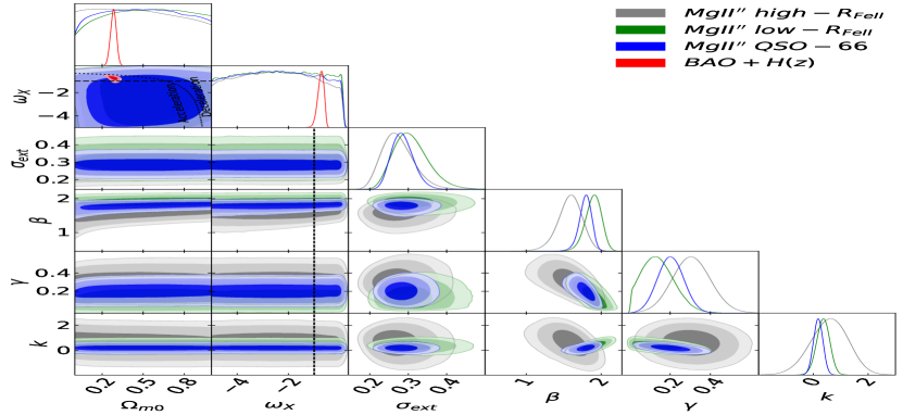
Refer to caption
Refer to caption
Refer to caption
Refer to caption
Refer to caption
Refer to caption
Figure 4: One-dimensional likelihood distributions and two-dimensional likelihood contours at 1σ𝜎\sigma, 2σ𝜎\sigma, and 3σ𝜎\sigma confidence levels using Mg ii high-FeiisubscriptFeii{\cal R}_{\rm{Fe\textsc{ii}}} (gray), Mg ii low-FeiisubscriptFeii{\cal R}_{\rm{Fe\textsc{ii}}} (green), Mg ii QSO-66 (blue), and BAO + H(z)𝐻𝑧H(z) (red) data for all free parameters. Left column shows the flat ΛΛ\LambdaCDM model, flat XCDM parametrization, and flat ϕitalic-ϕ\phiCDM model respectively. The black dotted lines in all plots are the zero acceleration lines. The black dashed lines in the flat XCDM parametrization plots are the ωX=1subscript𝜔𝑋1\omega_{X}=-1 lines. Right column shows the non-flat ΛΛ\LambdaCDM model, non-flat XCDM parametrization, and non-flat ϕitalic-ϕ\phiCDM model respectively. Black dotted lines in all plots are the zero acceleration lines. Black dashed lines in the non-flat ΛΛ\LambdaCDM and ϕitalic-ϕ\phiCDM model plots and black dotted-dashed lines in the non-flat XCDM parametrization plots correspond to Ωk0=0subscriptΩ𝑘00\Omega_{k0}=0. The black dashed lines in the non-flat XCDM parametrization plots are the ωX=1subscript𝜔𝑋1\omega_{X}=-1 lines.
Refer to caption
Refer to caption
Refer to caption
Refer to caption
Refer to caption
Refer to caption
Figure 5: One-dimensional likelihood distributions and two-dimensional likelihood contours at 1σ𝜎\sigma, 2σ𝜎\sigma, and 3σ𝜎\sigma confidence levels using Mg ii high-FeiisubscriptFeii{\cal R}_{\rm{Fe\textsc{ii}}} (gray), Mg ii low-FeiisubscriptFeii{\cal R}_{\rm{Fe\textsc{ii}}} (green), Mg ii QSO-66 (blue), and BAO + H(z)𝐻𝑧H(z) (red) data for all free parameters. Left column shows the flat ΛΛ\LambdaCDM model, flat XCDM parametrization, and flat ϕitalic-ϕ\phiCDM model respectively. The black dotted lines in all plots are the zero acceleration lines. The black dashed lines in the flat XCDM parametrization plots are the ωX=1subscript𝜔𝑋1\omega_{X}=-1 lines. Right column shows the non-flat ΛΛ\LambdaCDM model, non-flat XCDM parametrization, and non-flat ϕitalic-ϕ\phiCDM model respectively. Black dotted lines in all plots are the zero acceleration lines. Black dashed lines in the non-flat ΛΛ\LambdaCDM and ϕitalic-ϕ\phiCDM model plots and black dotted-dashed lines in the non-flat XCDM parametrization plots correspond to Ωk0=0subscriptΩ𝑘00\Omega_{k0}=0. The black dashed lines in the non-flat XCDM parametrization plots are the ωX=1subscript𝜔𝑋1\omega_{X}=-1 lines.
Refer to caption
Refer to caption
Refer to caption
Refer to caption
Refer to caption
Refer to caption
Figure 6: One-dimensional likelihood distributions and two-dimensional likelihood contours at 1σ𝜎\sigma, 2σ𝜎\sigma, and 3σ𝜎\sigma confidence levels using using Mg ii′′ high-FeiisubscriptFeii{\cal R}_{\rm{Fe\textsc{ii}}} (gray), Mg ii′′ low-FeiisubscriptFeii{\cal R}_{\rm{Fe\textsc{ii}}} (green), Mg ii′′ QSO-66 (blue), and BAO + H(z)𝐻𝑧H(z) (red) data for all free parameters. Left column shows the flat ΛΛ\LambdaCDM model, flat XCDM parametrization, and flat ϕitalic-ϕ\phiCDM model respectively. The black dotted lines in all plots are the zero acceleration lines. The black dashed lines in the flat XCDM parametrization plots are the ωX=1subscript𝜔𝑋1\omega_{X}=-1 lines. Right column shows the non-flat ΛΛ\LambdaCDM model, non-flat XCDM parametrization, and non-flat ϕitalic-ϕ\phiCDM model respectively. Black dotted lines in all plots are the zero acceleration lines. Black dashed lines in the non-flat ΛΛ\LambdaCDM and ϕitalic-ϕ\phiCDM model plots and black dotted-dashed lines in the non-flat XCDM parametrization plots correspond to Ωk0=0subscriptΩ𝑘00\Omega_{k0}=0. The black dashed lines in the non-flat XCDM parametrization plots are the ωX=1subscript𝜔𝑋1\omega_{X}=-1 lines.
Refer to caption
Refer to caption
Refer to caption
Refer to caption
Refer to caption
Refer to caption
Figure 7: One-dimensional likelihood distributions and two-dimensional likelihood contours at 1σ𝜎\sigma, 2σ𝜎\sigma, and 3σ𝜎\sigma confidence levels using using Mg ii QSO-66 (blue), Mg ii′′ QSO-66 (green), Mg ii QSO-66 (gray), and BAO + H(z)𝐻𝑧H(z) (red) data for all free parameters. Left column shows the flat ΛΛ\LambdaCDM model, flat XCDM parametrization, and flat ϕitalic-ϕ\phiCDM model respectively. The black dotted lines in all plots are the zero acceleration lines. The black dashed lines in the flat XCDM parametrization plots are the ωX=1subscript𝜔𝑋1\omega_{X}=-1 lines. Right column shows the non-flat ΛΛ\LambdaCDM model, non-flat XCDM parametrization, and non-flat ϕitalic-ϕ\phiCDM model respectively. Black dotted lines in all plots are the zero acceleration lines. Black dashed lines in the non-flat ΛΛ\LambdaCDM and ϕitalic-ϕ\phiCDM model plots and black dotted-dashed lines in the non-flat XCDM parametrization plots correspond to Ωk0=0subscriptΩ𝑘00\Omega_{k0}=0. The black dashed lines in the non-flat XCDM parametrization plots are the ωX=1subscript𝜔𝑋1\omega_{X}=-1 lines.
Refer to caption
Refer to caption
Refer to caption
Refer to caption
Refer to caption
Refer to caption
Figure 8: One-dimensional likelihood distributions and two-dimensional likelihood contours at 1σ𝜎\sigma, 2σ𝜎\sigma, and 3σ𝜎\sigma confidence levels using using Mg ii low-FeiisubscriptFeii{\cal R}_{\rm{Fe\textsc{ii}}} (blue), Mg ii′′ low-FeiisubscriptFeii{\cal R}_{\rm{Fe\textsc{ii}}} (green), Mg ii low-FeiisubscriptFeii{\cal R}_{\rm{Fe\textsc{ii}}} (gray), and BAO + H(z)𝐻𝑧H(z) (red) data for all free parameters. Left column shows the flat ΛΛ\LambdaCDM model, flat XCDM parametrization, and flat ϕitalic-ϕ\phiCDM model respectively. The black dotted lines in all plots are the zero acceleration lines. The black dashed lines in the flat XCDM parametrization plots are the ωX=1subscript𝜔𝑋1\omega_{X}=-1 lines. Right column shows the non-flat ΛΛ\LambdaCDM model, non-flat XCDM parametrization, and non-flat ϕitalic-ϕ\phiCDM model respectively. Black dotted lines in all plots are the zero acceleration lines. Black dashed lines in the non-flat ΛΛ\LambdaCDM and ϕitalic-ϕ\phiCDM model plots and black dotted-dashed lines in the non-flat XCDM parametrization plots correspond to Ωk0=0subscriptΩ𝑘00\Omega_{k0}=0. The black dashed lines in the non-flat XCDM parametrization plots are the ωX=1subscript𝜔𝑋1\omega_{X}=-1 lines.
Refer to caption
Refer to caption
Refer to caption
Refer to caption
Refer to caption
Refer to caption
Figure 9: One-dimensional likelihood distributions and two-dimensional likelihood contours at 1σ𝜎\sigma, 2σ𝜎\sigma, and 3σ𝜎\sigma confidence levels using using Mg ii high-FeiisubscriptFeii{\cal R}_{\rm{Fe\textsc{ii}}} (blue), Mg ii′′ high-FeiisubscriptFeii{\cal R}_{\rm{Fe\textsc{ii}}} (green), Mg ii high-FeiisubscriptFeii{\cal R}_{\rm{Fe\textsc{ii}}} (gray), and BAO + H(z)𝐻𝑧H(z) (red) data for all free parameters. Left column shows the flat ΛΛ\LambdaCDM model, flat XCDM parametrization, and flat ϕitalic-ϕ\phiCDM model respectively. The black dotted lines in all plots are the zero acceleration lines. The black dashed lines in the flat XCDM parametrization plots are the ωX=1subscript𝜔𝑋1\omega_{X}=-1 lines. Right column shows the non-flat ΛΛ\LambdaCDM model, non-flat XCDM parametrization, and non-flat ϕitalic-ϕ\phiCDM model respectively. Black dotted lines in all plots are the zero acceleration lines. Black dashed lines in the non-flat ΛΛ\LambdaCDM and ϕitalic-ϕ\phiCDM model plots and black dotted-dashed lines in the non-flat XCDM parametrization plots correspond to Ωk0=0subscriptΩ𝑘00\Omega_{k0}=0. The black dashed lines in the non-flat XCDM parametrization plots are the ωX=1subscript𝜔𝑋1\omega_{X}=-1 lines.
Table 4: Two-parameter RL𝑅𝐿R-L relation parameters (and σextsubscript𝜎ext\sigma_{\rm ext}) differences between the Mg ii low-FeiisubscriptFeii{\cal R}_{\rm{Fe\textsc{ii}}} and high-FeiisubscriptFeii{\cal R}_{\rm{Fe\textsc{ii}}} data sets.
Model ΔσextΔsubscript𝜎ext\Delta\sigma_{\rm ext} ΔγΔ𝛾\Delta\gamma ΔβΔ𝛽\Delta\beta
Flat ΛΛ\LambdaCDM 0.67σ0.67𝜎0.67\sigma 0.84σ0.84𝜎0.84\sigma 0.77σ0.77𝜎0.77\sigma
Non-flat ΛΛ\LambdaCDM 0.69σ0.69𝜎0.69\sigma 0.86σ0.86𝜎0.86\sigma 0.76σ0.76𝜎0.76\sigma
Flat XCDM 0.68σ0.68𝜎0.68\sigma 0.85σ0.85𝜎0.85\sigma 0.69σ0.69𝜎0.69\sigma
Non-flat XCDM 0.67σ0.67𝜎0.67\sigma 0.84σ0.84𝜎0.84\sigma 0.64σ0.64𝜎0.64\sigma
Flat ϕitalic-ϕ\phiCDM 0.67σ0.67𝜎0.67\sigma 0.84σ0.84𝜎0.84\sigma 0.76σ0.76𝜎0.76\sigma
Non-flat ϕitalic-ϕ\phiCDM 0.65σ0.65𝜎0.65\sigma 0.84σ0.84𝜎0.84\sigma 0.71σ0.71𝜎0.71\sigma
Table 5: Three-parameter linear-FeiisubscriptFeii{\cal R}_{\rm{Fe\textsc{ii}}} RL𝑅𝐿R-L relation parameters (and σextsubscript𝜎ext\sigma_{\rm ext}) differences between the Mg ii low-FeiisubscriptFeii{\cal R}_{\rm{Fe\textsc{ii}}} and high-FeiisubscriptFeii{\cal R}_{\rm{Fe\textsc{ii}}} data sets.
Model ΔσextΔsubscript𝜎ext\Delta\sigma_{\rm ext} ΔγΔ𝛾\Delta\gamma ΔβΔ𝛽\Delta\beta ΔkΔ𝑘\Delta k
Flat ΛΛ\LambdaCDM 0.67σ0.67𝜎0.67\sigma 1.18σ1.18𝜎1.18\sigma 0.61σ0.61𝜎0.61\sigma 0.23σ0.23𝜎0.23\sigma
Non-flat ΛΛ\LambdaCDM 0.69σ0.69𝜎0.69\sigma 1.19σ1.19𝜎1.19\sigma 0.57σ0.57𝜎0.57\sigma 0.27σ0.27𝜎0.27\sigma
Flat XCDM 0.67σ0.67𝜎0.67\sigma 1.19σ1.19𝜎1.19\sigma 0.63σ0.63𝜎0.63\sigma 0.23σ0.23𝜎0.23\sigma
Non-flat XCDM 0.65σ0.65𝜎0.65\sigma 1.17σ1.17𝜎1.17\sigma 0.54σ0.54𝜎0.54\sigma 0.23σ0.23𝜎0.23\sigma
Flat ϕitalic-ϕ\phiCDM 0.68σ0.68𝜎0.68\sigma 1.19σ1.19𝜎1.19\sigma 0.54σ0.54𝜎0.54\sigma 0.24σ0.24𝜎0.24\sigma
Non-flat ϕitalic-ϕ\phiCDM 0.69σ0.69𝜎0.69\sigma 1.19σ1.19𝜎1.19\sigma 0.54σ0.54𝜎0.54\sigma 0.24σ0.24𝜎0.24\sigma
Table 6: Three-parameter log-FeiisubscriptFeii{\cal R}_{\rm{Fe\textsc{ii}}} RL𝑅𝐿R-L relation parameters (and σextsubscript𝜎ext\sigma_{\rm ext}) differences between the Mg ii′′ low-FeiisubscriptFeii{\cal R}_{\rm{Fe\textsc{ii}}} and high-FeiisubscriptFeii{\cal R}_{\rm{Fe\textsc{ii}}} data sets.
Model ΔσextΔsubscript𝜎ext\Delta\sigma_{\rm ext} ΔγΔ𝛾\Delta\gamma ΔβΔ𝛽\Delta\beta ΔkΔ𝑘\Delta k
Flat ΛΛ\LambdaCDM 0.58σ0.58𝜎0.58\sigma 1.41σ1.41𝜎1.41\sigma 1.72σ1.72𝜎1.72\sigma 0.35σ0.35𝜎0.35\sigma
Non-flat ΛΛ\LambdaCDM 0.58σ0.58𝜎0.58\sigma 1.41σ1.41𝜎1.41\sigma 1.72σ1.72𝜎1.72\sigma 0.35σ0.35𝜎0.35\sigma
Flat XCDM 0.57σ0.57𝜎0.57\sigma 1.44σ1.44𝜎1.44\sigma 1.60σ1.60𝜎1.60\sigma 0.32σ0.32𝜎0.32\sigma
Non-flat XCDM 0.54σ0.54𝜎0.54\sigma 1.40σ1.40𝜎1.40\sigma 1.58σ1.58𝜎1.58\sigma 0.27σ0.27𝜎0.27\sigma
Flat ϕitalic-ϕ\phiCDM 0.57σ0.57𝜎0.57\sigma 1.44σ1.44𝜎1.44\sigma 1.78σ1.78𝜎1.78\sigma 0.31σ0.31𝜎0.31\sigma
Non-flat ϕitalic-ϕ\phiCDM 0.57σ0.57𝜎0.57\sigma 1.42σ1.42𝜎1.42\sigma 1.70σ1.70𝜎1.70\sigma 0.32σ0.32𝜎0.32\sigma

6 Discussion

In this paper we analyzed a sample of 66 Mg ii quasars with inferred UV FeiisubscriptFeii{\cal R}_{\rm{Fe\textsc{ii}}} ratios (or relative Fe ii strengths) that are meant to serve as accretion-rate proxies (Panda et al., 2019c; Śniegowska et al., 2020). We derived cosmological constraints using six cosmological models (flat and non-flat ΛΛ\LambdaCDM, ϕitalic-ϕ\phiCDM, and XCDM), and 2- and 3-parameter RL𝑅𝐿R-L relations, while considering the full Mg ii sample as well as two equally-sized subsamples of low- and high-FeiisubscriptFeii{\cal R}_{\rm{Fe\textsc{ii}}} sources, with 33 Mg ii sources in each subsample. We included the relative UV Fe ii strength in an attempt to correct for the accretion-rate effect. The cosmological constraints are in all cases consistent among the different samples as well as with constraints from better-established cosmological probes (BAO + H(z)𝐻𝑧H(z) data). The inclusion of the third parameter FeiisubscriptFeii{\cal R}_{\rm{Fe\textsc{ii}}} in the RL𝑅𝐿R-L relation does not result in the widely-expected reduction of the intrinsic scatter σextsubscript𝜎ext\sigma_{\rm ext}. In most cases the 2-parameter relation is mildly to positively preferred over the 3-parameter RL𝑅𝐿R-L relation, see Table LABEL:tab:1.

Previously, Khadka et al. (2021a) found for Hβ𝛽\beta quasars that including the optical FeiisubscriptFeii{\cal R}_{\rm{Fe\textsc{ii}}} parameter in a 3-parameter RL𝑅𝐿R-L relation also did not result in the widely-expected reduction of the intrinsic scatter. Moreover, in contrast to Mg ii quasars, low- and high-FeiisubscriptFeii{\cal R}_{\rm{Fe\textsc{ii}}} Hβ𝛽\beta sources obey different RL𝑅𝐿R-L relations, with the 3-parameter RL𝑅𝐿R-L relation being strongly favored over the 2-parameter one for the full sample of 118 sources, and with the inferred cosmological constraints being in 2σsimilar-toabsent2𝜎\sim 2\sigma tension with those found using better established cosmological probes.

There are several potential reasons for these differences between standardizable Mg ii quasars and Hβ𝛽\beta sources that may or may not be standardizable:

  • (i)

    For the sample of 66 Mg ii sources, low- and high-FeiisubscriptFeii{\cal R}_{\rm{Fe\textsc{ii}}} sources have consistent RL𝑅𝐿R-L relations and intrinsic scatter. In fact, high-FeiisubscriptFeii{\cal R}_{\rm{Fe\textsc{ii}}} Mg ii sources appear to have somewhat smaller scatter in comparison with that of the full sample as well as that of the low-FeiisubscriptFeii{\cal R}_{\rm{Fe\textsc{ii}}} sources (also see Martínez-Aldama et al., 2020b). This is unlike Hβ𝛽\beta sources where high-accretors exhibit a larger scatter with respect to low-FeiisubscriptFeii{\cal R}_{\rm{Fe\textsc{ii}}}  sources. (Martínez-Aldama et al., 2019; Du & Wang, 2019; Khadka et al., 2021a; Panda, 2022),

  • (ii)

    The sample of 66 Mg ii quasars used here is about a factor of 2 smaller than the Hβ𝛽\beta sample of 118 sources. The majority of the Mg ii sources, 57, are from the SDSS-reverberation-mapping (SDSS-RM) program (Homayouni et al., 2020) and cover a rather narrow range in monochromatic luminosity and rest-frame time-delay. The Hβ𝛽\beta sample of 118 sources is not only larger, but also more heterogeneous in terms of the time-delay determination methods.

  • (iii)

    Mg ii sources have a larger median redshift in comparison with the Hβ𝛽\beta quasars, z=0.990𝑧0.990z=0.990 vs. z=0.157𝑧0.157z=0.157, hence their redshifts are not significantly affected by peculiar velocities.

  • (iv)

    The UV region is not significantly affected by host starlight, which is the case for low-luminous Hβ𝛽\beta sources (Bentz et al., 2013). On the other hand, UV continuum emission may be prone to dust-extinction within their host galaxies and the intergalactic medium, but this effect is systematic for all Mg ii sources.

  • (v)

    Broad Hβ𝛽\beta and Mg ii lines are excited by different mechanisms: Hβ𝛽\beta is a recombination line, while Mg ii is a resonance line (Panda et al., 2019b; Śniegowska et al., 2020). Different photoionization mechanisms may account for some of the differences, such as the RL𝑅𝐿R-L relation slope, though a detailed analysis is beyond the scope of the current study. The Mg ii line is 20%similar-toabsentpercent20\sim 20\% narrower than the Hβ𝛽\beta line (Marziani et al., 2013) which hints at its position being farther away from the supermassive black hole. In addition, Yang et al. (2020) found that the Mg ii line responds to the variable continuum with a smaller amplitude, while the Mg ii line width does not significantly change with luminosity (lack of “breathing”), as Guo et al. (2020) found.

  • (vi)

    The smaller slope of the Mg ii-based RL𝑅𝐿R-L relation in comparison with both the Hβ𝛽\beta-based RL𝑅𝐿R-L correlation slope (Martínez-Aldama et al., 2019; Khadka et al., 2021a) and the slope predicted by simple photoionization theory (γionsubscript𝛾ion\gamma_{\rm ion}=0.5; Karas et al., 2021; Panda, 2022) is either caused by the source selection effect (cumulation of SDSS-RM sources at intermediate luminosities) or by the different photoionization mechanism and/or distribution of Mg ii-emitting gas (e.g. lack of the intrinsic “breathing” effect for Mg ii-emitting material; Guo et al., 2020; Wang et al., 2020).

The common feature for both Mg ii and Hβ𝛽\beta sources is that the inclusion of the third parameter, FeiisubscriptFeii{\cal R}_{\rm{Fe\textsc{ii}}}, in a 3-parameter RL𝑅𝐿R-L relation does not result in the widely-expected significant reduction of the intrinsic scatter (this paper and Khadka et al., 2021a). This may be due to the fact that the correlation between the Eddington ratio and the FeiisubscriptFeii{\cal R}_{\rm{Fe\textsc{ii}}}  parameter is generally not very strong (Zajaček et al., 2021) and/or the accretion-rate effect is not entirely responsible for the intrinsic scatter in the RL𝑅𝐿R-L relation.121212Du & Wang (2019) report a significant scatter reduction for their sample of Hβ𝛽\beta sources, going from σext0.28similar-tosubscript𝜎ext0.28\sigma_{\rm ext}\sim 0.28 to σext=0.196subscript𝜎ext0.196\sigma_{\rm ext}=0.196 after the inclusion of the optical FeiisubscriptFeii{\cal R}_{\rm{Fe\textsc{ii}}} parameter. This is, however, based on an approximate computation that only accounts for the variation in the RL𝑅𝐿R-L relation parameters and the intrinsic dispersion, while holding fixed all cosmological-model parameters (they adopted the flat ΛΛ\LambdaCDM model with H0=67kms1Mpc1subscript𝐻067kmsuperscripts1superscriptMpc1H_{0}=67\,{\rm km\,s^{-1}\,Mpc^{-1}}, ΩΛ=0.68subscriptΩΛ0.68\Omega_{\Lambda}=0.68, and Ωm0=0.32subscriptΩ𝑚00.32\Omega_{m0}=0.32), unlike the more complete computations done in Khadka et al. (2021a) and this paper. In addition, their sample size was smaller (75 vs. 118 sources) in comparison with Khadka et al. (2021a). The scatter is partially also driven by the time-delay uncertainties since the determination of the broad-line time-delay requires long enough monitoring to be reliable. Adding just a few extra years of monitoring can change the rest-frame time-delay by as much as a factor of two, as was the case for one of the Mg ii quasars CTS C30.10 (Czerny et al., 2019; Prince et al., 2022). This can be mitigated by continued monitoring of already reverberation-mapped sources and by enlarging the sample using extensive photometric and spectroscopic surveys of higher-redshift quasars.

7 Conclusion

We have investigated two 3-parameter RL𝑅𝐿R-L relations for Mg ii QSO sources. In our previous work with Mg II QSOs, we only studied the 2-parameter RL𝑅𝐿R-L relation (Khadka et al., 2021b) and found that the Mg ii QSO cosmological constraints were weak but consistent with cosmological constraints derived using better-established cosmological probes. Some discrepancies in the RL𝑅𝐿R-L relations of Hβ𝛽\beta QSOs (Khadka et al., 2021a), and the 2σsimilar-toabsent2𝜎\sim 2\sigma discrepancy between the Hβ𝛽\beta cosmological constraints and those derived using better-established cosmological probes, motivated our current paper.

We find here that for Mg ii data and the 2-parameter RL𝑅𝐿R-L relation, the low-FeiisubscriptFeii{\cal R}_{\rm{Fe\textsc{ii}}} and high-FeiisubscriptFeii{\cal R}_{\rm{Fe\textsc{ii}}} data subsets obey the same RL𝑅𝐿R-L relation within the error bars. This is strikingly different compared to what happens in the Hβ𝛽\beta QSO case (Khadka et al., 2021a) and is a positive result for the on-going development of Mg ii QSOs as cosmological probes. Our analyses with the 3-parameter RL𝑅𝐿R-L relations here show that the inclusion of the third parameter k𝑘k increases the RL𝑅𝐿R-L relation parameter differences between the low-FeiisubscriptFeii{\cal R}_{\rm{Fe\textsc{ii}}} and high-FeiisubscriptFeii{\cal R}_{\rm{Fe\textsc{ii}}} data subsets. This increase is not very significant for the linear-FeiisubscriptFeii{\cal R}_{\rm{Fe\textsc{ii}}} 3-parameter RL𝑅𝐿R-L relation in eq. (4) with q=𝑞absentq=FeiisubscriptFeii{\cal R}_{\rm{Fe\textsc{ii}}}  but is more significant for the log-FeiisubscriptFeii{\cal R}_{\rm{Fe\textsc{ii}}} 3-parameter RL𝑅𝐿R-L relation in eq. (4) with q=log𝑞q=\log{}FeiisubscriptFeii{\cal R}_{\rm{Fe\textsc{ii}}}. However, the motivation for extending the 2-parameter RL𝑅𝐿R-L relation to a 3-parameter one is the attempt to reduce the intrinsic dispersion of the RL𝑅𝐿R-L relation; our analyses here shows no evidence for this (and this is similar to what happens in the Hβ𝛽\beta case, Khadka et al., 2021a).131313In Khadka et al. (2021a) we found that for the full Hβ𝛽\beta data set the 3-parameter RL𝑅𝐿R-L relation provided a significantly better fit to data than did the 2-parameter RL𝑅𝐿R-L relation, unlike what we have found for Mg ii data here. This is because the Hβ𝛽\beta low-FeiisubscriptFeii{\cal R}_{\rm{Fe\textsc{ii}}} and high-FeiisubscriptFeii{\cal R}_{\rm{Fe\textsc{ii}}} data subsets obey very different 2-parameter RL𝑅𝐿R-L relations, unlike the case for Mg ii data here.

Unlike current Hβ𝛽\beta QSOs, current Mg ii QSOs consistently obey the 2-parameter RL𝑅𝐿R-L relation and so are standardizable and can be used as cosmological probes. It is important to continue to check whether this remains true for future Mg ii QSOs. If it does, and if there is a significant increase in the quantity and quality of reverberation-measured Mg ii time-lag QSOs over an extended redshift range, this will allow for tighter Mg ii cosmological constraints as well as a more definitive study of the adequacy of the 2-parameter RL𝑅𝐿R-L relation for Mg ii sources.

8 ACKNOWLEDGEMENTS

This research was supported in part by US DOE grant DE-SC0011840, by the Polish Funding Agency National Science Centre, project 2017/26/A/ST9/00756 (Maestro 9), by GAČR EXPRO grant 21-13491X, by Millenium Nucleus NCN19_05819_05819\_058 (TITANs), and by the Conselho Nacional de Desenvolvimento Científico e Tecnológico (CNPq) Fellowship (164753/2020-6). Part of the computation for this project was performed on the Beocat Research Cluster at Kansas State University.

Data availability

The data analysed in this article are listed in Table LABEL:tab:MgQSOdata of this paper.

References

  • Abdalla et al. (2022) Abdalla E., et al., 2022, arXiv e-prints, p. arXiv:2203.06142
  • Arjona & Nesseris (2021) Arjona R., Nesseris S., 2021, Phys. Rev. D, 103, 103539
  • Bentz et al. (2013) Bentz M. C., et al., 2013, ApJ, 767, 149
  • Brinckmann & Lesgourgues (2019) Brinckmann T., Lesgourgues J., 2019, Physics of the Dark Universe, 24, 100260
  • Cao & Ratra (2022) Cao S., Ratra B., 2022, arXiv e-prints, p. arXiv:2203.10825
  • Cao et al. (2017) Cao S., Zheng X., Biesiada M., Qi J., Chen Y., Zhu Z.-H., 2017, A&A, 606, A15
  • Cao et al. (2020) Cao S., Ryan J., Ratra B., 2020, MNRAS, 497, 3191
  • Cao et al. (2021a) Cao S., Ryan J., Khadka N., Ratra B., 2021a, MNRAS, 501, 1520
  • Cao et al. (2021b) Cao S., Ryan J., Ratra B., 2021b, MNRAS, 504, 300
  • Cao et al. (2022a) Cao S., Dainotti M., Ratra B., 2022a, arXiv e-prints, p. arXiv:2204.08710
  • Cao et al. (2022b) Cao S., Zajaček M., Panda S., Martínez-Aldama M. L., Czerny B., Ratra B., 2022b, arXiv e-prints, p. arXiv:2205.15552
  • Cao et al. (2022c) Cao S., Ryan J., Ratra B., 2022c, MNRAS, 509, 4745
  • Cao et al. (2022d) Cao S., Khadka N., Ratra B., 2022d, MNRAS, 510, 2928
  • Cao et al. (2022e) Cao S., Dainotti M., Ratra B., 2022e, MNRAS, 512, 439
  • Chávez et al. (2014) Chávez R., Terlevich R., Terlevich E., Bresolin F., Melnick J., Plionis M., Basilakos S., 2014, MNRAS, 442, 3565
  • Chen et al. (2016) Chen Y., Ratra B., Biesiada M., Li S., Zhu Z.-H., 2016, ApJ, 829, 61
  • Czerny et al. (2013) Czerny B., Hryniewicz K., Maity I., Schwarzenberg-Czerny A., Życki P. T., Bilicki M., 2013, A&A, 556, A97
  • Czerny et al. (2019) Czerny B., et al., 2019, ApJ, 880, 46
  • Czerny et al. (2021) Czerny B., et al., 2021, Acta Physica Polonica A, 139, 389
  • D’Agostini (2005) D’Agostini G., 2005, arXiv e-prints, p. physics/0511182
  • DES Collaboration (2019) DES Collaboration 2019, Phys. Rev. D, 99, 123505
  • Dainotti et al. (2022a) Dainotti M. G., Bardiacchi G., Lukasz Lenart A., Capozziello S., Colgain E. O., Solomon R., Stojkovic D., Sheikh-Jabbari M. M., 2022a, arXiv e-prints, p. arXiv:2203.12914
  • Dainotti et al. (2022b) Dainotti M. G., Nielson V., Sarracino G., Rinaldi E., Nagataki S., Capozziello S., Gnedin O. Y., Bargiacchi G., 2022b, arXiv e-prints, p. arXiv:2203.15538
  • de Cruz Perez et al. (2021) de Cruz Perez J., Sola Peracaula J., Gomez-Valent A., Moreno-Pulido C., 2021, preprint, (arXiv:2110.07569)
  • Demianski et al. (2021) Demianski M., Piedipalumbo E., Sawant D., Amati L., 2021, MNRAS, 506, 903
  • Dhawan et al. (2021) Dhawan S., Alsing J., Vagnozzi S., 2021, MNRAS, 506, L1
  • Di Valentino et al. (2021a) Di Valentino E., et al., 2021a, Classical and Quantum Gravity, 38, 153001
  • Di Valentino et al. (2021b) Di Valentino E., Melchiorri A., Silk J., 2021b, ApJ, 908, L9
  • Du & Wang (2019) Du P., Wang J.-M., 2019, ApJ, 886, 42
  • eBOSS Collaboration (2021) eBOSS Collaboration 2021, Phys. Rev. D, 103, 083533
  • Efstathiou & Gratton (2020) Efstathiou G., Gratton S., 2020, MNRAS, 496, L91
  • Fana Dirirsa et al. (2019) Fana Dirirsa F., et al., 2019, ApJ, 887, 13
  • Geng et al. (2022) Geng C.-Q., Hsu Y.-T., Lu J.-R., 2022, ApJ, 926, 74
  • González-Morán et al. (2021) González-Morán A. L., et al., 2021, MNRAS,
  • Guo et al. (2020) Guo H., et al., 2020, ApJ, 888, 58
  • Haas et al. (2011) Haas M., Chini R., Ramolla M., Pozo Nuñez F., Westhues C., Watermann R., Hoffmeister V., Murphy M., 2011, A&A, 535, A73
  • Homayouni et al. (2020) Homayouni Y., et al., 2020, ApJ, 901, 55
  • Hu et al. (2021) Hu J. P., Wang F. Y., Dai Z. G., 2021, MNRAS, 507, 730
  • Ichikawa et al. (2015) Ichikawa K., et al., 2015, ApJ, 803, 57
  • Jesus et al. (2021) Jesus J. F., Valentim R., Escobal A. A., Pereira S. H., Benndorf D., 2021, preprint, (arXiv:2112.09722)
  • Johnson et al. (2022) Johnson J. P., Sangwan A., Shankaranarayanan S., 2022, J. Cosmology Astropart. Phys., 2022, 024
  • Karas et al. (2021) Karas V., Svoboda J., Zajaček M., 2021, in RAGtime: Workshops on black holes and netron stars. p. E1 (arXiv:1901.06507)
  • Kaspi et al. (2000) Kaspi S., Smith P. S., Netzer H., Maoz D., Jannuzi B. T., Giveon U., 2000, ApJ, 533, 631
  • Khadka & Ratra (2020a) Khadka N., Ratra B., 2020a, MNRAS, 492, 4456
  • Khadka & Ratra (2020b) Khadka N., Ratra B., 2020b, MNRAS, 497, 263
  • Khadka & Ratra (2020c) Khadka N., Ratra B., 2020c, MNRAS, 499, 391
  • Khadka & Ratra (2021) Khadka N., Ratra B., 2021, MNRAS, 502, 6140
  • Khadka & Ratra (2022) Khadka N., Ratra B., 2022, MNRAS, 510, 2753
  • Khadka et al. (2021a) Khadka N., Martínez-Aldama M. L., Zajaček M., Czerny B., Ratra B., 2021a, arXiv e-prints, p. arXiv:2112.00052
  • Khadka et al. (2021b) Khadka N., Yu Z., Zajaček M., Martinez-Aldama M. L., Czerny B., Ratra B., 2021b, MNRAS, 508, 4722
  • Khadka et al. (2021c) Khadka N., Luongo O., Muccino M., Ratra B., 2021c, J. Cosmology Astropart. Phys., 2021, 042
  • KiDS Collaboration (2021) KiDS Collaboration 2021, A&A, 649, A88
  • Koratkar & Gaskell (1991) Koratkar A. P., Gaskell C. M., 1991, ApJ, 370, L61
  • Kozłowski (2015) Kozłowski S., 2015, Acta Astron., 65, 251
  • Lawrence & Elvis (2010) Lawrence A., Elvis M., 2010, ApJ, 714, 561
  • Lewis (2019) Lewis A., 2019, preprint, (arXiv:1910.13970)
  • Li et al. (2020) Li E.-K., Du M., Xu L., 2020, MNRAS, 491, 4960
  • Lian et al. (2021) Lian Y., Cao S., Biesiada M., Chen Y., Zhang Y., Guo W., 2021, MNRAS, 505, 2111–2123
  • Luongo & Muccino (2021) Luongo O., Muccino M., 2021, Galaxies, 9
  • Luongo et al. (2021) Luongo O., Muccino M., Colgáin E. Ó., Sheikh-Jabbari M. M., Yin L., 2021, preprint, (arXiv:2108.13228)
  • Lusso et al. (2020) Lusso E., et al., 2020, A&A, 642, A150
  • Mania & Ratra (2012) Mania D., Ratra B., 2012, Physics Letters B, 715, 9
  • Martínez-Aldama et al. (2019) Martínez-Aldama M. L., Czerny B., Kawka D., Karas V., Panda S., Zajaček M., Życki P. T., 2019, ApJ, 883, 170
  • Martinez Aldama et al. (2020a) Martinez Aldama M. L., Panda S., Czerny B., Zajacek M., LSST AGN SC Collaboration 2020a, in Multifrequency Behaviour of High Energy Cosmic Sources - XIII. 3-8 June 2019. Palermo. p. 10 (arXiv:1910.02725)
  • Martínez-Aldama et al. (2020b) Martínez-Aldama M. L., Zajaček M., Czerny B., Panda S., 2020b, ApJ, 903, 86
  • Marziani et al. (2013) Marziani P., Sulentic J. W., Plauchu-Frayn I., del Olmo A., 2013, A&A, 555, A89
  • Mehrabi et al. (2022) Mehrabi A., et al., 2022, MNRAS, 509, 224
  • Mejía-Restrepo et al. (2018) Mejía-Restrepo J. E., Lira P., Netzer H., Trakhtenbrot B., Capellupo D. M., 2018, Nature Astronomy, 2, 63
  • Mukherjee & Banerjee (2022) Mukherjee P., Banerjee N., 2022, Phys. Rev. D, 105, 063516
  • Netzer (2019) Netzer H., 2019, MNRAS, 488, 5185
  • Ooba et al. (2018a) Ooba J., Ratra B., Sugiyama N., 2018a, ApJ, 864, 80
  • Ooba et al. (2018b) Ooba J., Ratra B., Sugiyama N., 2018b, ApJ, 866, 68
  • Ooba et al. (2018c) Ooba J., Ratra B., Sugiyama N., 2018c, ApJ, 869, 34
  • Ooba et al. (2019) Ooba J., Ratra B., Sugiyama N., 2019, Ap&SS, 364, 176
  • Panda (2022) Panda S., 2022, Frontiers in Astronomy and Space Sciences, 9, 850409
  • Panda et al. (2019a) Panda S., Martínez-Aldama M. L., Zajaček M., 2019a, Frontiers in Astronomy and Space Sciences, 6, 75
  • Panda et al. (2019b) Panda S., Czerny B., Done C., Kubota A., 2019b, ApJ, 875, 133
  • Panda et al. (2019c) Panda S., Marziani P., Czerny B., 2019c, ApJ, 882, 79
  • Park & Ratra (2018) Park C.-G., Ratra B., 2018, ApJ, 868, 83
  • Park & Ratra (2019a) Park C.-G., Ratra B., 2019a, Ap&SS, 364, 82
  • Park & Ratra (2019b) Park C.-G., Ratra B., 2019b, Ap&SS, 364, 134
  • Park & Ratra (2019c) Park C.-G., Ratra B., 2019c, ApJ, 882, 158
  • Park & Ratra (2020) Park C.-G., Ratra B., 2020, Phys. Rev. D, 101, 083508
  • Pavlov et al. (2013) Pavlov A., Westmoreland S., Saaidi K., Ratra B., 2013, Phys. Rev. D, 88, 123513
  • Peebles (1984) Peebles P. J. E., 1984, ApJ, 284, 439
  • Peebles & Ratra (1988) Peebles P. J. E., Ratra B., 1988, ApJ, 325, L17
  • Perivolaropoulos & Skara (2021) Perivolaropoulos L., Skara F., 2021, preprint, (arXiv:2105.05208)
  • Peterson (1993) Peterson B. M., 1993, PASP, 105, 247
  • Planck Collaboration (2020) Planck Collaboration 2020, A&A, 641, A6
  • Prince et al. (2022) Prince R., et al., 2022, arXiv e-prints, p. arXiv:2201.11062
  • Rana et al. (2017) Rana A., Jain D., Mahajan S., Mukherjee A., 2017, J. Cosmology Astropart. Phys., 2017, 028
  • Ratra & Peebles (1988) Ratra B., Peebles P. J. E., 1988, Phys. Rev. D, 37, 3406
  • Renzi et al. (2021) Renzi F., Hogg N. B., Giarè W., 2021, preprint, (arXiv:2112.05701)
  • Rezaei et al. (2022) Rezaei M., Solà Peracaula J., Malekjani M., 2022, MNRAS, 509, 2593
  • Risaliti & Lusso (2015) Risaliti G., Lusso E., 2015, ApJ, 815, 33
  • Risaliti & Lusso (2019) Risaliti G., Lusso E., 2019, Nature Astronomy, 3, 272
  • Ryan et al. (2018) Ryan J., Doshi S., Ratra B., 2018, MNRAS, 480, 759
  • Ryan et al. (2019) Ryan J., Chen Y., Ratra B., 2019, MNRAS, 488, 3844
  • Scolnic et al. (2018) Scolnic D. M., et al., 2018, ApJ, 859, 101
  • Shen et al. (2016) Shen Y., et al., 2016, ApJ, 818, 30
  • Shen et al. (2019) Shen Y., et al., 2019, ApJS, 241, 34
  • Singh et al. (2019) Singh A., Sangwan A., Jassal H. K., 2019, J. Cosmology Astropart. Phys., 2019, 047
  • Sinha & Banerjee (2021) Sinha S., Banerjee N., 2021, J. Cosmology Astropart. Phys., 2021, 060
  • Śniegowska et al. (2020) Śniegowska M., Kozłowski S., Czerny B., Panda S., Hryniewicz K., 2020, ApJ, 900, 64
  • Solà Peracaula et al. (2019) Solà Peracaula J., Gómez-Valent A., de Cruz Pérez J., 2019, Physics of the Dark Universe, 25, 100311
  • Ureña-López & Roy (2020) Ureña-López L. A., Roy N., 2020, Phys. Rev. D, 102, 063510
  • Vagnozzi et al. (2021a) Vagnozzi S., Di Valentino E., Gariazzo S., Melchiorri A., Mena O., Silk J., 2021a, Physics of the Dark Universe, 33, 100851
  • Vagnozzi et al. (2021b) Vagnozzi S., Loeb A., Moresco M., 2021b, ApJ, 908, 84
  • Wang et al. (2014) Wang J.-M., et al., 2014, ApJ, 793, 108
  • Wang et al. (2016) Wang J. S., Wang F. Y., Cheng K. S., Dai Z. G., 2016, A&A, 585, A68
  • Wang et al. (2020) Wang S., et al., 2020, ApJ, 903, 51
  • Wang et al. (2022) Wang F. Y., Hu J. P., Zhang G. Q., Dai Z. G., 2022, ApJ, 924, 97
  • Watson et al. (2011) Watson D., Denney K. D., Vestergaard M., Davis T. M., 2011, ApJ, 740, L49
  • Wei (2018) Wei J.-J., 2018, ApJ, 868, 29
  • Wei & Melia (2022) Wei J.-J., Melia F., 2022, ApJ, 928, 165
  • Xu et al. (2021) Xu T., Chen Y., Xu L., Cao S., 2021, preprint, (arXiv:2109.02453)
  • Yang et al. (2020) Yang Q., et al., 2020, MNRAS, 493, 5773
  • Yu et al. (2018) Yu H., Ratra B., Wang F.-Y., 2018, ApJ, 856, 3
  • Yu et al. (2021) Yu Z., et al., 2021, arXiv e-prints, p. arXiv:2103.01973
  • Zajaček et al. (2020) Zajaček M., et al., 2020, ApJ, 896, 146
  • Zajaček et al. (2021) Zajaček M., et al., 2021, ApJ, 912, 10
  • Zhai et al. (2017) Zhai Z., Blanton M., Slosar A., Tinker J., 2017, ApJ, 850, 183
  • Zheng et al. (2021) Zheng X., Cao S., Biesiada M., Li X., Liu T., Liu Y., 2021, Science China Physics, Mechanics, and Astronomy, 64, 259511

Appendix A Mg ii QSO data

Table 7: Reverberation-measured Mg ii QSO data. For each source, columns list: QSO name, redshift, continuum flux density at 3000 Å, measured rest-frame time-delay, the ratio of the UV Fe ii  flux density with respect to the MgII flux density FeiisubscriptFeii{\cal R}_{\rm{Fe\textsc{ii}}}, the original source reference, and the FeiisubscriptFeii{\cal R}_{\rm{Fe\textsc{ii}}} class where number 1 corresponds to low-FeiisubscriptFeii{\cal R}_{\rm{Fe\textsc{ii}}} sources (FeiisubscriptFeii{\cal R}_{\rm{Fe\textsc{ii}}}<1.0467absent1.0467<1.0467) and number 2 to high-FeiisubscriptFeii{\cal R}_{\rm{Fe\textsc{ii}}} sources (FeiisubscriptFeii{\cal R}_{\rm{Fe\textsc{ii}}}>1.0467absent1.0467>1.0467). The first 65 sources were analyzed by Martínez-Aldama et al. (2020b), the last source HE 0435-4312 is from Zajaček et al. (2021). The references are designated as follows: (a) stands for sources taken from Homayouni et al. (2020) (in total 57 source, where the object number corresponds to the RMID number from the original catalogue); (b) Shen et al. (2016); (c) Shen et al. (2019); (d) Czerny et al. (2019); (e) Prince et al. (2022); (f) Zajaček et al. (2020); (g) monochromatic luminosity inferred following Kozłowski (2015); (h) Zajaček et al. (2021).
Object z𝑧z log(F3000/ergs1cm2)subscript𝐹3000ergsuperscripts1superscriptcm2\log\left(F_{3000}/{\rm erg}\,{\rm s^{-1}}{\rm cm^{-2}}\right) log(L3000/ergs1)subscript𝐿3000ergsuperscripts1\log\left(L_{3000}/{\rm erg}\,{\rm s^{-1}}\right) τ𝜏\tau (day) FeiisubscriptFeii{\cal R}_{\rm{Fe\textsc{ii}}} Ref. FeiisubscriptFeii{\cal R}_{\rm{Fe\textsc{ii}}} class
018 0.848 13.1081±0.0009plus-or-minus13.10810.0009-13.1081\pm 0.0009 44.4331±0.0009plus-or-minus44.43310.000944.4331\pm 0.0009 125.97.0+6.8subscriptsuperscript125.96.87.0125.9^{+6.8}_{-7.0} 0.4716±0.0194plus-or-minus0.47160.01940.4716\pm 0.0194 (a) 1
028 1.392 12.4342±0.0004plus-or-minus12.43420.0004-12.4342\pm 0.0004 45.6391±0.0004plus-or-minus45.63910.000445.6391\pm 0.0004 65.714.2+24.8subscriptsuperscript65.724.814.265.7^{+24.8}_{-14.2} 1.0340±0.0134plus-or-minus1.03400.01341.0340\pm 0.0134 (a) 1
038 1.383 12.3956±0.0003plus-or-minus12.39560.0003-12.3956\pm 0.0003 45.6707±0.0003plus-or-minus45.67070.000345.6707\pm 0.0003 120.728.7+27.9subscriptsuperscript120.727.928.7120.7^{+27.9}_{-28.7} 1.2057±0.0152plus-or-minus1.20570.01521.2057\pm 0.0152 (a) 2
044 1.233 13.0287±0.0013plus-or-minus13.02870.0013-13.0287\pm 0.0013 44.9143±0.0013plus-or-minus44.91430.001344.9143\pm 0.0013 65.84.8+18.8subscriptsuperscript65.818.84.865.8^{+18.8}_{-4.8} 1.0594±0.0644plus-or-minus1.05940.06441.0594\pm 0.0644 (a) 2
102 0.861 12.5513±0.0005plus-or-minus12.55130.0005-12.5513\pm 0.0005 45.0061±0.0005plus-or-minus45.00610.000545.0061\pm 0.0005 86.913.3+16.2subscriptsuperscript86.916.213.386.9^{+16.2}_{-13.3} 1.4152±0.0259plus-or-minus1.41520.02591.4152\pm 0.0259 (a) 2
114 1.226 11.8682±0.0003plus-or-minus11.86820.0003-11.8682\pm 0.0003 46.0687±0.0003plus-or-minus46.06870.000346.0687\pm 0.0003 186.615.4+20.3subscriptsuperscript186.620.315.4186.6^{+20.3}_{-15.4} 1.3508±0.0399plus-or-minus1.35080.03991.3508\pm 0.0399 (a) 2
118 0.715 12.2374±0.0006plus-or-minus12.23740.0006-12.2374\pm 0.0006 45.1217±0.0006plus-or-minus45.12170.000645.1217\pm 0.0006 102.219.5+27.0subscriptsuperscript102.227.019.5102.2^{+27.0}_{-19.5} 1.2126±0.0270plus-or-minus1.21260.02701.2126\pm 0.0270 (a) 2
123 0.891 12.9147±0.0009plus-or-minus12.91470.0009-12.9147\pm 0.0009 44.6794±0.0009plus-or-minus44.67940.000944.6794\pm 0.0009 81.626.6+28.0subscriptsuperscript81.628.026.681.6^{+28.0}_{-26.6} 1.1069±0.325plus-or-minus1.10690.3251.1069\pm 0.325 (a) 2
135 1.315 12.7843±0.0005plus-or-minus12.78430.0005-12.7843\pm 0.0005 45.2279±0.0005plus-or-minus45.22790.000545.2279\pm 0.0005 93.09.8+9.6subscriptsuperscript93.09.69.893.0^{+9.6}_{-9.8} 1.0785±0.0097plus-or-minus1.07850.00971.0785\pm 0.0097 (a) 2
158 1.478 13.2009±0.0012plus-or-minus13.20090.0012-13.2009\pm 0.0012 44.9367±0.0012plus-or-minus44.93670.001244.9367\pm 0.0012 119.111.8+4.0subscriptsuperscript119.14.011.8119.1^{+4.0}_{-11.8} 0.9489±0.0211plus-or-minus0.94890.02110.9489\pm 0.0211 (a) 1
159 1.587 12.7115±0.0006plus-or-minus12.71150.0006-12.7115\pm 0.0006 45.5023±0.0006plus-or-minus45.50230.000645.5023\pm 0.0006 324.219.4+25.3subscriptsuperscript324.225.319.4324.2^{+25.3}_{-19.4} 1.0098±0.0180plus-or-minus1.00980.01801.0098\pm 0.0180 (a) 1
160 0.36 12.8476±0.0013plus-or-minus12.84760.0013-12.8476\pm 0.0013 43.7965±0.0013plus-or-minus43.79650.001343.7965\pm 0.0013 106.516.6+18.2subscriptsuperscript106.518.216.6106.5^{+18.2}_{-16.6} 0.2622±0.0055plus-or-minus0.26220.00550.2622\pm 0.0055 (a) 1
170 1.163 12.6724±0.0005plus-or-minus12.67240.0005-12.6724\pm 0.0005 45.2078±0.0005plus-or-minus45.20780.000545.2078\pm 0.0005 98.517.7+6.7subscriptsuperscript98.56.717.798.5^{+6.7}_{-17.7} 0.7566±0.0109plus-or-minus0.75660.01090.7566\pm 0.0109 (a) 1
185 0.987 12.8520±0.0094plus-or-minus12.85200.0094-12.8520\pm 0.0094 44.8519±0.0094plus-or-minus44.85190.009444.8519\pm 0.0094 387.93.0+3.3subscriptsuperscript387.93.33.0387.9^{+3.3}_{-3.0} 1.2979±0.3264plus-or-minus1.29790.32641.2979\pm 0.3264 (a) 2
191 0.442 13.0675±0.0012plus-or-minus13.06750.0012-13.0675\pm 0.0012 43.7869±0.0012plus-or-minus43.78690.001243.7869\pm 0.0012 93.929.1+24.3subscriptsuperscript93.924.329.193.9^{+24.3}_{-29.1} 0.6649±0.0339plus-or-minus0.66490.03390.6649\pm 0.0339 (a) 1
228 1.264 13.2425±0.0011plus-or-minus13.24250.0011-13.2425\pm 0.0011 44.7272±0.0011plus-or-minus44.72720.001144.7272\pm 0.0011 37.99.1+14.4subscriptsuperscript37.914.49.137.9^{+14.4}_{-9.1} 1.0697±0.0420plus-or-minus1.06970.04201.0697\pm 0.0420 (a) 2
232 0.808 13.2316±0.0014plus-or-minus13.23160.0014-13.2316\pm 0.0014 44.2579±0.0014plus-or-minus44.25790.001444.2579\pm 0.0014 273.84.1+5.1subscriptsuperscript273.85.14.1273.8^{+5.1}_{-4.1} 1.0113±0.0901plus-or-minus1.01130.09011.0113\pm 0.0901 (a) 1
240 0.762 13.3448±0.0021plus-or-minus13.34480.0021-13.3448\pm 0.0021 44.0821±0.0021plus-or-minus44.08210.002144.0821\pm 0.0021 17.22.8+3.5subscriptsuperscript17.23.52.817.2^{+3.5}_{-2.8} 0.6603±0.0276plus-or-minus0.66030.02760.6603\pm 0.0276 (a) 1
260 0.995 12.4492±0.0004plus-or-minus12.44920.0004-12.4492\pm 0.0004 45.2633±0.0004plus-or-minus45.26330.000445.2633\pm 0.0004 94.917.2+18.7subscriptsuperscript94.918.717.294.9^{+18.7}_{-17.2} 0.9968±0.0182plus-or-minus0.99680.01820.9968\pm 0.0182 (a) 1
280 1.366 12.5521±0.0003plus-or-minus12.55210.0003-12.5521\pm 0.0003 45.5009±0.0003plus-or-minus45.50090.000345.5009\pm 0.0003 99.19.5+3.3subscriptsuperscript99.13.39.599.1^{+3.3}_{-9.5} 1.0222±0.0145plus-or-minus1.02220.01451.0222\pm 0.0145 (a) 1
285 1.034 13.2726±0.0020plus-or-minus13.27260.0020-13.2726\pm 0.0020 44.4812±0.0020plus-or-minus44.48120.002044.4812\pm 0.0020 138.521.1+15.2subscriptsuperscript138.515.221.1138.5^{+15.2}_{-21.1} 0.5753±0.0189plus-or-minus0.57530.01890.5753\pm 0.0189 (a) 1
291 0.532 13.2325±0.0016plus-or-minus13.23250.0016-13.2325\pm 0.0016 43.8146±0.0016plus-or-minus43.81460.001643.8146\pm 0.0016 39.72.6+4.2subscriptsuperscript39.74.22.639.7^{+4.2}_{-2.6} 0.1551±0.0118plus-or-minus0.15510.01180.1551\pm 0.0118 (a) 1
294 1.215 12.4673±0.0004plus-or-minus12.46730.0004-12.4673\pm 0.0004 45.4599±0.0004plus-or-minus45.45990.000445.4599\pm 0.0004 71.89.5+17.8subscriptsuperscript71.817.89.571.8^{+17.8}_{-9.5} 1.3498±0.0247plus-or-minus1.34980.02471.3498\pm 0.0247 (a) 2
301 0.548 12.8427±0.0011plus-or-minus12.84270.0011-12.8427\pm 0.0011 44.2355±0.0011plus-or-minus44.23550.001144.2355\pm 0.0011 136.316.9+17.0subscriptsuperscript136.317.016.9136.3^{+17.0}_{-16.9} 0.7894±0.0270plus-or-minus0.78940.02700.7894\pm 0.0270 (a) 1
303 0.821 13.2805±0.0013plus-or-minus13.28050.0013-13.2805\pm 0.0013 44.2261±0.0013plus-or-minus44.22610.001344.2261\pm 0.0013 57.78.3+10.5subscriptsuperscript57.710.58.357.7^{+10.5}_{-8.3} 0.8923±0.0170plus-or-minus0.89230.01700.8923\pm 0.0170 (a) 1
329 0.721 11.9688±0.0007plus-or-minus11.96880.0007-11.9688\pm 0.0007 45.3992±0.0007plus-or-minus45.39920.000745.3992\pm 0.0007 87.514.0+23.8subscriptsuperscript87.523.814.087.5^{+23.8}_{-14.0} 1.5348±0.0333plus-or-minus1.53480.03331.5348\pm 0.0333 (a) 2
338 0.418 13.0371±0.0013plus-or-minus13.03710.0013-13.0371\pm 0.0013 43.7598±0.0013plus-or-minus43.75980.001343.7598\pm 0.0013 22.16.2+8.8subscriptsuperscript22.18.86.222.1^{+8.8}_{-6.2} 0.1975±0.0190plus-or-minus0.19750.01900.1975\pm 0.0190 (a) 1
419 1.272 12.9275±0.0011plus-or-minus12.92750.0011-12.9275\pm 0.0011 45.0489±0.0011plus-or-minus45.04890.001145.0489\pm 0.0011 95.515.5+15.2subscriptsuperscript95.515.215.595.5^{+15.2}_{-15.5} 1.1103±0.0257plus-or-minus1.11030.02571.1103\pm 0.0257 (a) 2
422 1.074 13.0888±0.0011plus-or-minus13.08880.0011-13.0888\pm 0.0011 44.7058±0.0011plus-or-minus44.70580.001144.7058\pm 0.0011 109.329.6+25.4subscriptsuperscript109.325.429.6109.3^{+25.4}_{-29.6} 0.3254±0.0073plus-or-minus0.32540.00730.3254\pm 0.0073 (a) 1
440 0.754 12.4820±0.0004plus-or-minus12.48200.0004-12.4820\pm 0.0004 44.9337±0.0004plus-or-minus44.93370.000444.9337\pm 0.0004 114.610.8+7.4subscriptsuperscript114.67.410.8114.6^{+7.4}_{-10.8} 0.9773±0.0139plus-or-minus0.97730.01390.9773\pm 0.0139 (a) 1
441 1.397 12.6008±0.0004plus-or-minus12.60080.0004-12.6008\pm 0.0004 45.4763±0.0004plus-or-minus45.47630.000445.4763\pm 0.0004 127.77.3+5.7subscriptsuperscript127.75.77.3127.7^{+5.7}_{-7.3} 1.3191±0.0424plus-or-minus1.31910.04241.3191\pm 0.0424 (a) 2
449 1.218 12.9573±0.0013plus-or-minus12.95730.0013-12.9573\pm 0.0013 44.9725±0.0013plus-or-minus44.97250.001344.9725\pm 0.0013 119.824.4+14.7subscriptsuperscript119.814.724.4119.8^{+14.7}_{-24.4} 1.1464±0.0336plus-or-minus1.14640.03361.1464\pm 0.0336 (a) 2
457 0.604 13.4931±0.0029plus-or-minus13.49310.0029-13.4931\pm 0.0029 43.6874±0.0029plus-or-minus43.68740.002943.6874\pm 0.0029 20.505.3+7.7subscriptsuperscript20.507.75.320.50^{+7.7}_{-5.3} 0.2002±0.0283plus-or-minus0.20020.02830.2002\pm 0.0283 (a) 1
459 1.156 12.8865±0.0011plus-or-minus12.88650.0011-12.8865\pm 0.0011 44.9872±0.0011plus-or-minus44.98720.001144.9872\pm 0.0011 122.85.7+5.1subscriptsuperscript122.85.15.7122.8^{+5.1}_{-5.7} 1.0102±0.0346plus-or-minus1.01020.03461.0102\pm 0.0346 (a) 1
469 1.004 12.1473±0.0002plus-or-minus12.14730.0002-12.1473\pm 0.0002 45.5749±0.0002plus-or-minus45.57490.000245.5749\pm 0.0002 224.174.3+27.9subscriptsuperscript224.127.974.3224.1^{+27.9}_{-74.3} 1.2398±0.0295plus-or-minus1.23980.02951.2398\pm 0.0295 (a) 2
492 0.964 12.3949±0.0004plus-or-minus12.39490.0004-12.3949\pm 0.0004 45.2837±0.0004plus-or-minus45.28370.000445.2837\pm 0.0004 92.012.7+16.3subscriptsuperscript92.016.312.792.0^{+16.3}_{-12.7} 1.0328±0.0167plus-or-minus1.03280.01671.0328\pm 0.0167 (a) 1
493 1.592 12.2609±0.0004plus-or-minus12.26090.0004-12.2609\pm 0.0004 45.9563±0.0004plus-or-minus45.95630.000445.9563\pm 0.0004 315.635.7+30.7subscriptsuperscript315.630.735.7315.6^{+30.7}_{-35.7} 1.3944±0.0360plus-or-minus1.39440.03601.3944\pm 0.0360 (a) 2
501 1.155 12.9605±0.0009plus-or-minus12.96050.0009-12.9605\pm 0.0009 44.9123±0.0009plus-or-minus44.91230.000944.9123\pm 0.0009 44.910.4+11.7subscriptsuperscript44.911.710.444.9^{+11.7}_{-10.4} 1.0066±0.0444plus-or-minus1.00660.04441.0066\pm 0.0444 (a) 1
505 1.144 13.0664±0.0011plus-or-minus13.06640.0011-13.0664\pm 0.0011 44.7961±0.0011plus-or-minus44.79610.001144.7961\pm 0.0011 94.716.7+10.8subscriptsuperscript94.710.816.794.7^{+10.8}_{-16.7} 0.8675±0.0209plus-or-minus0.86750.02090.8675\pm 0.0209 (a) 1
522 1.384 12.9840±0.0006plus-or-minus12.98400.0006-12.9840\pm 0.0006 45.0831±0.0006plus-or-minus45.08310.000645.0831\pm 0.0006 115.816.0+11.3subscriptsuperscript115.811.316.0115.8^{+11.3}_{-16.0} 1.2665±0.0320plus-or-minus1.26650.03201.2665\pm 0.0320 (a) 2
556 1.494 12.6554±0.0005plus-or-minus12.65540.0005-12.6554\pm 0.0005 45.4937±0.0005plus-or-minus45.49370.000545.4937\pm 0.0005 98.710.8+13.9subscriptsuperscript98.713.910.898.7^{+13.9}_{-10.8} 1.2118±0.0164plus-or-minus1.21180.01641.2118\pm 0.0164 (a) 2
588 0.998 12.1342±0.0002plus-or-minus12.13420.0002-12.1342\pm 0.0002 45.5816±0.0002plus-or-minus45.58160.000245.5816\pm 0.0002 74.318.2+23.0subscriptsuperscript74.323.018.274.3^{+23.0}_{-18.2} 1.0015±0.0125plus-or-minus1.00150.01251.0015\pm 0.0125 (a) 1
593 0.992 12.7386±0.0006plus-or-minus12.73860.0006-12.7386\pm 0.0006 44.9707±0.0006plus-or-minus44.97070.000644.9707\pm 0.0006 80.120.8+21.4subscriptsuperscript80.121.420.880.1^{+21.4}_{-20.8} 1.0595±0.0176plus-or-minus1.05950.01761.0595\pm 0.0176 (a) 2
622 0.572 12.6271±0.0005plus-or-minus12.62710.0005-12.6271\pm 0.0005 44.4961±0.0005plus-or-minus44.49610.000544.4961\pm 0.0005 61.74.3+6.0subscriptsuperscript61.76.04.361.7^{+6.0}_{-4.3} 1.7362±0.0368plus-or-minus1.73620.03681.7362\pm 0.0368 (a) 2
645 0.474 12.7685±0.0009plus-or-minus12.76850.0009-12.7685\pm 0.0009 44.1583±0.0009plus-or-minus44.15830.000944.1583\pm 0.0009 30.28.9+26.8subscriptsuperscript30.226.88.930.2^{+26.8}_{-8.9} 1.3497±0.0440plus-or-minus1.34970.04401.3497\pm 0.0440 (a) 2
649 0.85 13.0933±0.0013plus-or-minus13.09330.0013-13.0933\pm 0.0013 44.4504±0.0013plus-or-minus44.45040.001344.4504\pm 0.0013 165.525.1+22.2subscriptsuperscript165.522.225.1165.5^{+22.2}_{-25.1} 2.3486±0.3300plus-or-minus2.34860.33002.3486\pm 0.3300 (a) 2
651 1.486 12.9595±0.0011plus-or-minus12.95950.0011-12.9595\pm 0.0011 45.1839±0.0011plus-or-minus45.18390.001145.1839\pm 0.0011 76.515.6+18.0subscriptsuperscript76.518.015.676.5^{+18.0}_{-15.6} 0.8697±0.0216plus-or-minus0.86970.02160.8697\pm 0.0216 (a) 1
675 0.919 12.5484±0.0005plus-or-minus12.54840.0005-12.5484\pm 0.0005 45.0789±0.0005plus-or-minus45.07890.000545.0789\pm 0.0005 139.822.6+12.0subscriptsuperscript139.812.022.6139.8^{+12.0}_{-22.6} 1.2550±0.0146plus-or-minus1.25500.01461.2550\pm 0.0146 (a) 2
678 1.463 12.8283±0.0007plus-or-minus12.82830.0007-12.8283\pm 0.0007 45.2983±0.0007plus-or-minus45.29830.000745.2983\pm 0.0007 82.910.2+11.9subscriptsuperscript82.911.910.282.9^{+11.9}_{-10.2} 1.1805±0.0254plus-or-minus1.18050.02541.1805\pm 0.0254 (a) 2
709 1.251 12.9770±0.0010plus-or-minus12.97700.0010-12.9770\pm 0.0010 44.9816±0.0010plus-or-minus44.98160.001044.9816\pm 0.0010 85.419.3+17.7subscriptsuperscript85.417.719.385.4^{+17.7}_{-19.3} 1.3036±0.0475plus-or-minus1.30360.04751.3036\pm 0.0475 (a) 2
714 0.921 12.8414±0.0012plus-or-minus12.84140.0012-12.8414\pm 0.0012 44.7882±0.0012plus-or-minus44.78820.001244.7882\pm 0.0012 320.111.2+11.3subscriptsuperscript320.111.311.2320.1^{+11.3}_{-11.2} 0.5856±0.0216plus-or-minus0.58560.02160.5856\pm 0.0216 (a) 1
756 0.852 13.1449±0.0023plus-or-minus13.14490.0023-13.1449\pm 0.0023 44.4013±0.0023plus-or-minus44.40130.002344.4013\pm 0.0023 315.316.4+20.5subscriptsuperscript315.320.516.4315.3^{+20.5}_{-16.4} 1.2265±0.0345plus-or-minus1.22650.03451.2265\pm 0.0345 (a) 2
761 0.771 12.6558±0.0024plus-or-minus12.65580.0024-12.6558\pm 0.0024 44.7837±0.0024plus-or-minus44.78370.002444.7837\pm 0.0024 102.17.4+8.2subscriptsuperscript102.18.27.4102.1^{+8.2}_{-7.4} 1.4789±0.0420plus-or-minus1.47890.04201.4789\pm 0.0420 (a) 2
771 1.492 12.4571±0.0004plus-or-minus12.45710.0004-12.4571\pm 0.0004 45.6906±0.0004plus-or-minus45.69060.000445.6906\pm 0.0004 31.34.6+8.1subscriptsuperscript31.38.14.631.3^{+8.1}_{-4.6} 0.7654±0.0084plus-or-minus0.76540.00840.7654\pm 0.0084 (a) 1
774 1.686 12.5769±0.0004plus-or-minus12.57690.0004-12.5769\pm 0.0004 45.7017±0.0004plus-or-minus45.70170.000445.7017\pm 0.0004 58.910.1+13.7subscriptsuperscript58.913.710.158.9^{+13.7}_{-10.1} 1.1880±0.0306plus-or-minus1.18800.03061.1880\pm 0.0306 (a) 2
792 0.526 13.4922±0.0030plus-or-minus13.49220.0030-13.4922\pm 0.0030 43.5431±0.0030plus-or-minus43.54310.003043.5431\pm 0.0030 111.420.0+29.5subscriptsuperscript111.429.520.0111.4^{+29.5}_{-20.0} 0.6261±0.1034plus-or-minus0.62610.10340.6261\pm 0.1034 (a) 1
848 0.757 13.3426±0.0015plus-or-minus13.34260.0015-13.3426\pm 0.0015 44.0773±0.0015plus-or-minus44.07730.001544.0773\pm 0.0015 65.116.3+29.4subscriptsuperscript65.129.416.365.1^{+29.4}_{-16.3} 0.8990±0.0584plus-or-minus0.89900.05840.8990\pm 0.0584 (a) 1
J141214.20++532546.7 0.45810 12.2526±0.0004plus-or-minus12.25260.0004-12.2526\pm 0.0004 44.6388±0.0004plus-or-minus44.63880.000444.6388\pm 0.0004 36.74.8+10.4subscriptsuperscript36.710.44.836.7^{+10.4}_{-4.8} 1.650±0.201plus-or-minus1.6500.2011.650\pm 0.201 (b), (c) 2
J141018.04++532937.5 0.4696 13.1883±0.0051plus-or-minus13.18830.0051-13.1883\pm 0.0051 43.7288±0.0051plus-or-minus43.72880.005143.7288\pm 0.0051 32.35.3+12.9subscriptsuperscript32.312.95.332.3^{+12.9}_{-5.3} 0.900±0.085plus-or-minus0.9000.0850.900\pm 0.085 (b), (c) 1
J141417.13++515722.6 0.6037 13.4925±0.0029plus-or-minus13.49250.0029-13.4925\pm 0.0029 43.6874±0.0029plus-or-minus43.68740.002943.6874\pm 0.0029 29.18.8+3.6subscriptsuperscript29.13.68.829.1^{+3.6}_{-8.8} 0.200±0.028plus-or-minus0.2000.0280.200\pm 0.028 (b), (c) 1
J142049.28++521053.3 0.751 12.7205±0.0009plus-or-minus12.72050.0009-12.7205\pm 0.0009 44.6909±0.0009plus-or-minus44.69090.000944.6909\pm 0.0009 34.012.0+6.7subscriptsuperscript34.06.712.034.0^{+6.7}_{-12.0} 1.450±0.034plus-or-minus1.4500.0341.450\pm 0.034 (b), (c) 2
J141650.93++535157.0 0.5266 13.2587±0.0020plus-or-minus13.25870.0020-13.2587\pm 0.0020 43.7778±0.0020plus-or-minus43.77780.002043.7778\pm 0.0020 25.12.6+2.0subscriptsuperscript25.12.02.625.1^{+2.0}_{-2.6} 0.100±0.011plus-or-minus0.1000.0110.100\pm 0.011 (b), (c) 1
J141644.17++532556.1 0.4253 12.8668±0.0010plus-or-minus12.86680.0010-12.8668\pm 0.0010 43.9479±0.0010plus-or-minus43.94790.001043.9479\pm 0.0010 17.22.7+2.7subscriptsuperscript17.22.72.717.2^{+2.7}_{-2.7} 1.450±0.068plus-or-minus1.4500.0681.450\pm 0.068 (b), (c) 2
CTS C30.10 0.9005 11.5825±0.0260plus-or-minus11.58250.0260-11.5825\pm 0.0260 46.0230±0.0260plus-or-minus46.02300.026046.0230\pm 0.0260 275.519.5+12.4subscriptsuperscript275.512.419.5275.5^{+12.4}_{-19.5} 1.600±0.004plus-or-minus1.6000.0041.600\pm 0.004 (d), (e) 2
HE0413-4031 1.3765 11.3302±0.0824plus-or-minus11.33020.0824-11.3302\pm 0.0824 46.7310±0.0810plus-or-minus46.73100.081046.7310\pm 0.0810 302.919.1+23.7subscriptsuperscript302.923.719.1302.9^{+23.7}_{-19.1} 0.800±0.020plus-or-minus0.8000.0200.800\pm 0.020 (f), (g) 1
HE0435-4312 1.2231 11.5853±0.0361plus-or-minus11.58530.0361-11.5853\pm 0.0361 46.3490±0.0360plus-or-minus46.34900.036046.3490\pm 0.0360 29614.0+13.0subscriptsuperscript29613.014.0296^{+13.0}_{-14.0} 2.36±0.03plus-or-minus2.360.032.36\pm 0.03 (h), (g) 2
Table 7: continued.