Impact of Charge on the Complexity of Static Sphere in $f(R,\textbf{T}^{2})$ Gravity

Abstract

This paper investigates the complexity of a charged static sphere filled with anisotropic matter in the background of energy-momentum squared gravity. For this purpose, we evaluate the modified field and conservation equations to determine the structure of celestial system. The mass function is calculated through Misner-Sharp as well as Tolman mass definitions. The complexity of a self-gravitating system depends on different factors such as anisotropic pressure, electromagnetic field, energy density inhomogeneity, etc. We formulate the structure scalars by the orthogonal decomposition of the Riemann tensor to develop a complexity factor containing all vital features of the stellar structure. The vanishing complexity condition is achieved by setting the complexity factor equal to zero. Finally, we construct two static solutions by utilizing the energy density of Gokhroo-Mehra solution as well as the polytropic equation of state along with the zero complexity condition. It is found that electromagnetic field decreases the complexity of stellar structure.

Keywords: Energy-momentum squared gravity; Complexity factor; Polytropic equation of state.
PACS: 04.20.Jb; 04.40.Dg; 04.50.Kd

1 Introduction

Several astronomical observations from various experiments (Two-degree Field Galaxy Redshift, Survey Sloan Digital Sky Survey, Large Synoptic Survey Telescope) prove that the large scale structures such as galaxies and stars give vital information about the origin and evolution of the vast universe. Therefore, the study of these compact structures play a significant role in understanding the mechanism and origin of the cosmos. These self-gravitating structures are complex in nature as they comprise of organized and inter-linked components that collaborate in different ways. A slight perturbation in the complicated system may cause principal changes within the physical attributes of the stellar structure. To analyze the complicated nature and evolution of the astrophysical structure, it is mandatory to define a complexity factor that connects the essential physical parameters. Moreover, an effective complexity factor must measure how the internal and external perturbations affect the stability and evolution of stellar structures.

Numerous researchers have put a lot of efforts in determining an appropriate definition of complexity in different divisions of science [1]. However, a standard definition that is applicable in all fields has not been accomplished. In the earlier definitions of complexity, the idea of data and entropy were taken into account. However, these definitions were unable to precisely evaluate the complexity of the basic physical models: ideal gas and perfect crystal. In order to describe the symmetric distribution of particles in the perfect crystal, minimal data is sufficient. On the other hand, in case of ideal gas, maximal information is needed to indicate any of its likely state. Although these two states display a contrasting behavior, both are allotted the least complexity. Therefore, the definition of complexity must include factors other than entropy and information.

Lopez-Ruiz et al. [2] extended the idea of complexity by examining the concept of disequilibrium which is the difference between various probabilistic states and the equiprobable configuration of the structure. Researchers have replaced the probability distribution (used in defining the disequilibrium and information) by the energy density of the system to compute the complexity of self-gravitating structures like neutron stars and white dwarfs [3]. Dense stellar systems have particles that are compactly arranged in their interior. Consequently, less radial pressure is generated as compared to the tangential pressure which produces anisotropy in pressure. Thus, the anisotropy is an essential factor in determining the stability of a compact structure. As the idea of complexity suggested by Lopez-Ruiz and his collaborators dealt with energy density only while other state variables such as pressure and anisotropy were neglected, therefore, it does not define an effective criterion to measure complexity.

Recently, Herrera [4] established a new factor of complexity for static spherically symmetric structure in the background of general relativity (GR). The structure of the spherical system was examined in terms of state determinants such as anisotropic pressure, energy density, etc. The basic assumption was that a static matter distribution with homogeneous density and isotropic pressure constituted the simplest system. Consequently, the complexity factor for such a distribution is zero. Herrera utilized the Tolman mass to relate inhomogeneous energy density and pressure anisotropy through a single relation. He developed a complexity factor for self-gravitating anisotropic source by utilizing Bel’s technique for orthogonal decomposition of the Riemann tensor. Sharif and Butt [5] examined the complexity of the static cylindrical self-gravitating system by employing Herrera’s approach. Herrera et al. [6] also discussed the complexity of a dynamical spherically symmetric fluid distribution following a homologous pattern of evolution. This definition has been extended to axially symmetric static case by formulating three complexity factors [7]. Recently, Herrera et al. [8] explored a quasi-homologous self-gravitating structure satisfying the zero complexity condition.

The electromagnetic field is an essential factor in the evolution and stability of self-gravitating objects as it overcomes the attractive gravitational force. In astrophysics, the Reissner-Nordström metric was the first static spherically symmetric charged solution to the Einstein-Maxwell field equations. Rosseland and Eddington [9] studied the characteristics of charged fluid in the interior of self-gravitating spherically symmetric structures. Ray et al. [10] investigated the effect of electromagnetic field on compact stellar structure and deduced that the local impact of forces exerted on single charged particle created an imbalance of forces which ultimately generated a charged black hole. Sharif and Bhatti [11] investigated the stability of charged sphere filled with viscous dissipative matter and discussed the stability regions for collapsing systems through the adiabatic index. The stability of spherically symmetric anisotropic polytrope under the impact of electromagnetic field was checked by Sharif and Sadiq [12]. Sharif and Butt formulated the structures scalars by adopting Herrera’s technique and calculated the complexity factors for charged spherical [13] as well as cylindrical [14] self-gravitating systems. They concluded that the electromagnetic field decreases the complexity of stellar structures.

According to cosmic observations from numerous surveys (Type Ia Supernovae [15], Cosmic Microwave Background Radiation [16], Large Scale Structure [17], Baryon Acoustic Oscillations [18] and Sloan Digital Sky Survey [19]), our universe is undergoing accelerated expansion. This accelerated expansion is supposed to be the result of some mysterious force known as dark energy that has large negative pressure. Two different methods have been employed by researchers to determine the cause of cosmic expansion. First approach requires the modification of the energy-momentum tensor while the other way is to alter the geometric part in the Einstein-Hilbert action which leads to modified theories of relativity.

In GR, $\Lambda$ Cold Dark Matter model is used to successfully describe the evolution of the cosmos. However, it has some issues namely fine-tuning and coincidence problems. Thus, modified theories like $f(R),~{}f(R,T)$, etc. ($R$ denotes the Ricci scalar and $T$ is the trace of energy-momentum tensor $T_{\mu\nu}$) have gained the attention of researchers to deal with issues related to cosmic acceleration. The $f(R)$ theory is achieved by replacing $R$ with the generic function $f(R)$ in the Einstein-Hilbert action [20]. Harko et al. [21] proposed the $f(R,T)$ theory (an extension of $f(R)$ theory) by considering a gravitational Lagrangian density in terms of $R$ and $T$. The curvature-matter coupling models in $f(R,T)$ theory are valuable for describing the late-time cosmic acceleration as well as the interconnection of dark energy and dark matter [22]. A systematic review of some standard issues and also the latest developments of modified gravity in cosmology is given in [23]. The measure of complexity, introduced by Herrera, has also been developed in the context of these modified theories. Abbas and Nazar computed the complexity factor in $f(R)$ gravity for static [24] as well as dynamical [25] fluid distribution. Abbas and Ahmad [26] analyzed the complexity for a class of compact stars in $f(R,T)$ scenario. Herrera’s technique to formulate complexity factor has also been applied in other modified theories of gravity [27]. Several other works studying compact objects in modified gravity can be seen in [28].

Recently, Katrici and Kavuk [29] proposed a new generalization of GR by defining a specific coupling between matter and gravity through a term proportional to $T^{\mu\nu}T_{\mu\nu}$. This theory is referred to as energy-momentum squared gravity (EMSG) or $f(R,\textbf{T}^{2})$ theory with $\textbf{T}^{2}=T^{\mu\nu}T_{\mu\nu}$. The predictions of GR about singularities at high energy levels (such as big bang singularity) are no longer valid due to expected quantum effects. In this respect, EMSG is considered as a favorable framework because it resolves the big bang singularity by supporting regular bounce with finite maximum energy density and least scale factor in the beginning of the cosmos. The conservation law does not hold in EMSG due to interaction between matter and curvature which indicates the presence of some extra force. Consequently, the path of the test particle differs from the standard geodesic path. Various astrophysical and cosmological structures have been studied in $f(R,\textbf{T}^{2})$ theory.

Roshan and Shojai [30] obtained the exact solution of EMSG field equations and determined the possibility of bounce at an early time by applying $f(R,\textbf{T}^{2})$ theory to homogeneous and isotropic spacetime. Broad and Barrow [31] studied exact solutions representing the isotropic universe for different forms of $f(R,\textbf{T}^{2})$ and discussed their behavior with reference to various physical parameters. Some astrophysical objects such as neutron stars were examined in the background of EMSG with $f(R,\textbf{T}^{2})=R+\zeta T^{\mu\nu}T_{\mu\nu}$, $\zeta$ being a constant [32]. Bahamonde et al. [33] examined the dynamics of two different models to explain the current accelerated cosmic expansion. Sharif and Gul [34] explored the structure of cosmic objects through the Noether symmetry approach. They also studied the dynamics of cylindrical collapse with dissipative matter in the presence of charge and deduced that the dissipative matter, electromagnetic field and modified terms reduce the collapse rate [35].

The objective of this article is to develop the vanishing complexity condition for a static spherical distribution in the presence of charge within $f(R,\textbf{T}^{2})$ background. The layout of the paper is as follows. In the next section, we formulate the EMSG field equations for an anisotropic matter distribution. We discuss some physical attributes of matter distribution in section 3. In section 4, structure scalars are constructed by decomposing the curvature tensor with the help of four-velocity. In section 5, we formulate the zero complexity condition to produce solutions of modified field equations corresponding to an assumed energy density as well as polytropic equation of state. Finally, in section 6 we summarize the main results.

2 Field Equations

In this section, we will describe some physical variables related to charged spherical stellar structure and obtain the corresponding field equations. The modified Einstein-Hilbert action in $f(R,\textbf{T}^{2})$ gravity is given as [29]

$$S=\int(\mathcal{L}_{m}+\mathcal{L}_{e})\sqrt{-g}d^{4}x+\int\frac{f(R,\textbf{T}^{2})}{2\kappa^{2}}\sqrt{-g}d^{4}x,$$ (1)

where $g,~{}\mathcal{L}_{m},~{}\mathcal{L}_{e}$ and $\kappa$ are the determinant of the metric tensor ($g_{\mu\nu}$), matter Lagrangian, Lagrangian for the electromagnetic field and coupling constant, respectively. Here $\mathcal{L}_{e}$ has the form

$$\mathcal{L}_{e}=-\frac{1}{16\pi}\mathit{F}^{\mu\nu}\mathit{F}_{\mu\nu},$$

where the Maxwell field tensor $\mathit{F}_{\mu\nu}$ is defined as $\mathit{F}_{\mu\nu}=\phi_{\nu,\mu}-\phi_{\mu,\nu}$ and $\phi_{a}=\phi\delta^{0}_{a}$ with $\phi$ as the scalar field potential. The EMSG field equations obtained by varying Eq.(1) are

$$R_{\mu\nu}f_{R}+g_{\mu\nu}\Box f_{R}-\nabla_{\mu}\nabla_{\nu}f_{R}-\frac{1}{2}g_{\mu\nu}f=\kappa^{2}T_{\mu\nu}+E_{\mu\nu}-\Theta_{\mu\nu}f_{\textbf{T}^{2}},$$ (2)

where $R_{\mu\nu}$ denotes the Ricci tensor. Also, $\Box=\nabla^{\mu}\nabla_{\mu}$, $f_{R}=\frac{\partial f}{\partial R}$ and $f_{\textbf{T}^{2}}=\frac{\partial f}{\partial\textbf{T}^{2}}$. Here ${E}_{\mu\nu}$ is the electromagnetic field tensor and $\Theta_{\mu\nu}$ is given as

$$\Theta_{\mu\nu}=\frac{\delta\textbf{T}^{2}}{\delta g^{\mu\nu}}=\frac{\delta(T^{\mu\nu}T_{\mu\nu})}{\delta g^{\mu\nu}} = -2\mathcal{L}_{m}(T_{\mu\nu}-\frac{1}{2}g_{\mu\nu}T)-4\frac{\partial^{2}\mathcal{L}_{m}}{\partial g^{\mu\nu}\partial g^{\alpha\beta}}T^{\alpha\beta}$$ (3)

$$- TT_{\mu\nu}+2T^{\alpha}_{\mu}T_{\nu\alpha}.$$

The energy-momentum tensor related to the anisotropic fluid distribution is expressed as

$$T^{\mu}_{\nu}=\rho\emph{v}^{\mu}\emph{v}_{\nu}-\emph{p}\emph{h}^{\mu}_{\nu}+\Pi^{\mu}_{\nu}.$$ (4)

Here $\emph{v}_{\mu},~{}\emph{p},~{}\rho$ and $\Pi_{\mu\nu}$ denote the four-velocity, pressure, energy density and anisotropic tensor, respectively. These terms are defined as

$$\Pi^{\mu}_{\nu}=\frac{\Pi}{3}(3\emph{s}^{\mu}\emph{s}_{\nu}+\emph{h}^{\mu}_{\nu}),\quad\Pi=\emph{p}_{r}-\emph{p}_{\bot},\quad\emph{h}^{\mu}_{\nu}=\delta^{\mu}_{\nu}-\emph{v}^{\mu}\emph{v}_{\nu},~{}\emph{p}=\frac{1}{3}(\emph{p}_{r}+2\emph{p}_{\bot}),$$

where $\emph{p}_{r}$ and $\emph{p}_{\bot}$ are the radial and tangential pressures of anisotropic fluid, respectively. As matter Lagrangian has no specific definition, therefore, different matter Lagrangians produce different forms of the field equations. More widely used forms of matter Lagrangian are $\mathcal{L}_{m}=-\emph{p}$ and $\mathcal{L}_{m}=\rho$. These choices do not pose any problem in GR. However, for non-minimal coupling case, different forms of matter Lagrangian correspond to distinct results [36]. Thus, for our convenience, we consider $\mathcal{L}_{m}=\rho$ and $\kappa=1$ which yields [37]

$$\Theta_{\mu\nu} = -2\rho(T_{\mu\nu}-\frac{1}{2}g_{\mu\nu}T)-TT_{\mu\nu}+2T^{\alpha}_{\mu}T_{\nu\alpha},$$

$$\mathbb{G}_{\mu\nu} = R_{\mu\nu}-\frac{1}{2}Rg_{\mu\nu}=\frac{1}{\kappa^{2}f_{R}}(T^{(C)}_{\mu\nu}+T_{\mu\nu}+\emph{E}_{\mu\nu})=T^{(D)}_{\mu\nu},$$ (5)

where $\mathbb{G}_{\mu\nu}$ is the Einstein tensor and $T^{(C)}_{\mu\nu}$ are the modified terms of $f(R,\textbf{T}^{2})$ gravity (also called correction terms) takes the form

$$T^{(C)}_{\mu\nu} = \frac{1}{f_{R}}\bigg{\{}g_{\mu\nu}\left(\frac{f-R\ f_{R}}{2}\right)+(\nabla_{\mu}\nabla_{\nu}f_{R}-g_{\mu\nu}\Box f_{R})-\rho g_{\mu\nu}f_{\textbf{T}^{2}}T$$ (6)

$$+ (T+2\rho)f_{\textbf{T}^{2}}T_{\mu\nu}-2T^{\alpha}_{\mu}T_{\alpha\nu}f_{\textbf{T}^{2}}\bigg{\}}.$$

The role of charge is determined through the electromagnetic energy-momentum tensor given as

$${E}_{\mu\nu}=\frac{1}{4\pi}\left(\mathit{F}^{\alpha}_{\mu}\mathit{F}_{\nu\alpha}-\frac{1}{4}g_{\mu\nu}\mathit{F}^{\alpha\beta}\mathit{F}_{\alpha\beta}\right).$$

The tensorial formulation of Maxwell field equations is given as

$$\mathit{F}_{[\mu\nu;\lambda]}=0,\quad\mathit{F}^{\mu\nu}_{;\nu}=\mu_{o}\emph{J}^{\mu}.$$

where $\mu_{o}$ is the magnetic permeability. The electromagnetic four-current vector is defined as $\emph{J}_{i}=\frac{\sigma}{\sqrt{g_{00}}}\frac{\emph{d}x_{i}}{\emph{d}x^{4}}=\sigma\emph{v}_{i}$, where $\sigma$ is the charge density.

To analyze the compact structure, we consider the static spherical spacetime as

$$\emph{ds}^{2}=\mathcal{F}^{2}(r)\emph{dt}^{2}-\mathcal{G}^{2}(r)\emph{dr}^{2}-\emph{r}^{2}\emph{d}\theta^{2}-\emph{r}^{2}\sin^{2}\theta\emph{d}\Phi^{2}.$$ (7)

Consequently, the four-vector and four-velocity have the following forms

$$\emph{s}^{\mu}=(0,\frac{1}{\mathcal{G}},0,0),~{}\emph{v}^{\mu}=(\frac{1}{\mathcal{F}},0,0,0),$$

which imply that $\emph{v}_{\mu}\emph{v}^{\mu}=1,~{}\emph{s}_{\mu}\emph{s}^{\mu}=-1,~{}\emph{v}_{\mu}\emph{s}^{\mu}=0$. The Maxwell field equations for the considered metric turn out to be

$$\phi^{{}^{\prime\prime}}+(\frac{2}{r}-\frac{\mathcal{F}^{{}^{\prime}}}{\mathcal{F}}-\frac{\mathcal{G}^{{}^{\prime}}}{\mathcal{G}})\phi^{{}^{\prime}}=4\pi\sigma\mathcal{F}\mathcal{G}^{2},$$

where prime denotes derivative with respect to $r$. The integration of the above equation yields

$$\phi^{{}^{\prime}}=\frac{\mathcal{F}\mathcal{G}\emph{q}(r)}{r^{2}},$$

where the total charge within the sphere is given by $\emph{q}(r)=4\pi\int^{r}_{0}\sigma\mathcal{G}r^{2}\emph{d}r$. Taking covariant differentiation of Eq.(2), we obtain

$$\kappa^{2}\nabla^{\mu}T^{(D)}_{\mu\nu}=\nabla^{\mu}(\Theta_{\mu\nu}f_{\textbf{T}^{2}})-\frac{1}{2}g_{\mu\nu}\nabla^{\mu}f,$$ (8)

which implies that conservation of the energy-momentum tensor does not hold leading to the existence of an unknown force that causes non-geodesic movement of particles. The EMSG field equations corresponding to the line element in Eq.(7) are

$$\frac{1}{r^{2}}-\frac{1}{\mathcal{G}^{2}}\left(\frac{1}{r^{2}}-\frac{2\mathcal{G}^{{}^{\prime}}}{r\mathcal{G}}\right) = \frac{1}{f_{R}}\left(\rho+\varphi+\varphi_{00}-2\pi\mathbb{E}^{2}\right),$$ (9)

$$-\frac{1}{r^{2}}+\frac{1}{\mathcal{G}^{2}}\left(\frac{1}{r^{2}}+\frac{2\mathcal{F}^{{}^{\prime}}}{r\mathcal{F}}\right) = \frac{1}{f_{R}}\left\{(\emph{p}_{r}-\varphi+\varphi_{11})+\left(\rho^{2}+2\rho\emph{p}_{r}\right.\right.$$

$$- \left.\left.2\rho\emph{p}_{\bot}+\emph{p}^{2}_{r}-2\emph{p}_{r}\emph{p}_{\bot}\right)f_{\textbf{T}^{2}}+2\pi\mathbb{E}^{2}\right\},$$

$$\frac{1}{\mathcal{G}^{2}}\left(\frac{\mathcal{F}^{{}^{\prime\prime}}}{\mathcal{F}}-\frac{\mathcal{F}^{{}^{\prime}}\mathcal{G}^{{}^{\prime}}}{\mathcal{F}\mathcal{G}}\right)-\frac{1}{r\mathcal{G}^{2}}\left(\frac{\mathcal{G}^{{}^{\prime}}}{\mathcal{G}}-\frac{\mathcal{F}}{\mathcal{F}}\right) = \frac{1}{f_{R}}\left\{(\emph{p}_{\bot}-\varphi+\varphi_{22})+\left(\rho^{2}-\rho\emph{p}_{r}\right.\right.$$ (11)

$$+ \left.\left.\rho\emph{p}_{\bot}-\emph{p}_{r}\emph{p}_{\bot}\right)f_{\textbf{T}^{2}}-2\pi\mathbb{E}^{2}\right\},$$

where

$$\varphi = \frac{f-Rf_{R}}{2},$$

$$\varphi_{00} = -\frac{f^{{}^{\prime\prime}}_{R}}{\mathcal{G}^{2}}-\frac{1}{\mathcal{G}^{2}}\left(\frac{2}{r}-\frac{\mathcal{G}^{{}^{\prime}}}{\mathcal{G}}\right),$$

$$\varphi_{11} = -\frac{f^{{}^{\prime}}_{R}\mathcal{F}^{{}^{\prime}}}{\mathcal{F}\mathcal{G}^{2}}-\frac{2f^{{}^{\prime}}_{R}}{r\mathcal{G}^{2}},$$

$$\varphi_{22} = -\frac{1}{\mathcal{G}^{2}}\left\{f^{{}^{\prime\prime}}_{R}+\left(\frac{\mathcal{F}^{{}^{\prime}}}{\mathcal{F}}-\frac{\mathcal{G}^{{}^{\prime}}}{\mathcal{G}}+\frac{1}{r}\right)f^{{}^{\prime}}_{R}\right\},$$

$$\mathbb{E} = \frac{\emph{q}(r)}{4\pi r^{2}},$$

where $\mathbb{E}$ is the electric field intensity.

3 Physical Characteristics of Matter Distribution

The Riemann tensor measures the curvature of spacetime and is represented through the Ricci tensor, Ricci scalar and Weyl tensor ($\mathcal{C}^{\varepsilon}_{\mu\nu\lambda}$) as

$$R^{\varepsilon}_{\mu\nu\lambda}=\mathcal{C}^{\varepsilon}_{\mu\nu\lambda}+\frac{1}{2}R^{\varepsilon}_{\nu}g_{\mu\lambda}-\frac{1}{2}R_{\mu\nu}\delta^{\varepsilon}_{\lambda}+\frac{1}{2}R_{\mu\lambda}\delta^{\varepsilon}_{\nu}-\frac{1}{2}R^{\varepsilon}_{\lambda}g_{\mu\nu}-\frac{1}{6}R\left(\delta^{\varepsilon}_{\nu}g_{\mu\lambda}-g_{\mu\nu}\delta^{\varepsilon}_{\lambda}\right).$$ (12)

The Weyl tensor is the traceless component of the Riemann tensor which gauges the tidal constrain on a body. Utilizing the observer’s four-velocity, it can be decomposed into magnetic ($\mathcal{H}_{\mu\nu}$) and electric ($\mathcal{E}_{\mu\nu}$) parts as

$$\mathcal{H}_{\mu\nu}=\frac{1}{2}\eta_{\mu\alpha\varepsilon\beta}\mathcal{C}^{\varepsilon\beta}_{\nu\sigma}\emph{v}^{\alpha}\emph{v}^{\sigma},~{}\mathcal{E}_{\mu\nu}=\mathcal{C}_{\mu\lambda\nu\gamma}\emph{v}^{\lambda}\emph{v}^{\gamma}.$$

Here $\eta_{\alpha\beta\mu\nu}$ represents the Levi-Civita tensor, $g_{\iota\beta\lambda\nu}=g_{\iota\lambda}g_{\beta\nu}-g_{\iota\nu}g_{\beta\lambda}$ and $\mathcal{C}_{\alpha\beta\epsilon\sigma}=(g_{\alpha\beta\mu\nu}g_{\pi\lambda\kappa\varrho}-\eta_{\alpha\beta\mu\nu}\eta_{\pi\lambda\kappa\varrho})\emph{v}^{\mu}\emph{v}^{\kappa}\mathcal{E}^{\nu\varrho}$. For a spherically symmetric system, the magnetic part of the Weyl tensor varnishes whereas the electric component is written in terms of unit four-vector and projection tensor as

$$\mathcal{E}_{\mu\nu}=\mathcal{E}\left(\emph{s}_{\mu}\emph{s}_{\nu}+\frac{1}{3}\emph{h}_{\mu\nu}\right),$$ (13)

where $\mathcal{E}=-\frac{1}{2\mathcal{F}\mathcal{G}^{3}r^{2}}\left(\mathcal{F}^{{}^{\prime\prime}}\mathcal{G}r^{2}-\mathcal{F}^{{}^{\prime}}\mathcal{G}^{{}^{\prime}}r^{2}-\mathcal{F}\mathcal{G}^{3}+\mathcal{F}\mathcal{G}^{{}^{\prime}}r-\mathcal{F}^{{}^{\prime}}\mathcal{G}r+\mathcal{F}\mathcal{G}\right)$ with $\mathcal{E}^{\mu}_{\mu}\\ =0,~{}\mathcal{E}_{(\epsilon\delta)}=\mathcal{E}_{\epsilon\delta}$ and $\mathcal{E}_{\mu\lambda}\emph{v}^{\lambda}=0$.

Utilizing the definitions of Misner-Sharp [38] and Tolman mass [39], we develop an association between the Weyl tensor and mass function to explore some characteristics of the spherical framework. The mass obtained through Misner-Sharp as well as Tolman’s definitions has the same values at the boundary. However, these definitions provide the same estimates of mass within the interior in the scenario of isotropic and homogeneous fluid only. The formulation developed by Misner and Sharp under the impact of charge is given as

$$\frac{2}{r}\emph{m} = R^{2}_{232}=\left(1-\frac{1}{\mathcal{G}^{2}}\right)=\frac{1}{r}\int^{r}_{0}T^{(D)0}_{0}\tilde{r}^{2}\emph{d}\tilde{r}=\frac{1}{r}\int^{r}_{0}\frac{1}{f_{R}}\big{(}\rho+\varphi+\varphi_{00}$$ (14)

$$- 2\pi\mathbb{E}^{2}\big{)}\tilde{r}^{2}\emph{d}\tilde{r}.$$

Using the field equations along with Eq.(13), the mass function is rewritten as

m $$= r^{3}\left[\frac{1}{6f_{R}}\Big{\{}(\rho-\emph{p}_{r}+\emph{p}_{\bot})+(\varphi+\varphi_{00}-\varphi_{11}-\varphi_{22}-6\pi\mathbb{E}^{2})\right.$$ (15)

$$+ \left.(3\rho\emph{p}_{\bot}-3\rho\emph{p}_{r}+\emph{p}_{r}\emph{p}_{\bot}-\emph{p}^{2}_{r})f_{\textbf{T}^{2}}+\frac{\mathcal{E}}{3}\Big{\}}\right].$$

Equation (15) along with (14) leads to

$$\mathcal{E} = -\frac{1}{2r^{3}}\int^{r}_{0}\tilde{r}^{3}\bigg{\{}\left(\frac{1}{f_{R}}\right)^{{}^{\prime}}(\rho+\varphi+\varphi_{00}-2\pi\mathbb{E}^{2})+\left(\frac{1}{f_{R}}\right)\left(\rho+\varphi\right.$$ (16)

$$+ \left.\varphi_{00}-2\pi\mathbb{E}^{2})^{{}^{\prime}}\right)\bigg{\}}\emph{d}\tilde{r}+\frac{1}{2f_{R}}\Big{\{}(\emph{p}_{r}-\emph{p}_{\bot})+(\varphi_{11}-\varphi_{22}-4\pi\mathbb{E}^{2})$$

$$+ (3\rho\emph{p}_{r}-3\rho\emph{p}_{\bot}-\emph{p}_{r}\emph{p}_{\bot}+\emph{p}^{2}_{r})f_{\textbf{T}^{2}}\Big{\}}.$$

The above expression describes how Weyl tensor and physical properties of the fluid (anisotropic pressure, inhomogeneous energy density and total charge) are interlinked. Inserting Eq.(16) in (15) yields

$$\emph{m}(r) = \frac{r^{3}}{6}T^{(D)0}_{0}-\frac{1}{6}\int^{r}_{0}\tilde{r}^{3}\bigg{\{}\left(\frac{1}{f_{R}}\right)^{{}^{\prime}}(\rho+\varphi+\varphi_{00}-2\pi\mathbb{E}^{2})+\left(\frac{1}{f_{R}}\right)\big{(}\rho+\varphi$$ (17)

$$+ \varphi_{00}-2\pi\mathbb{E}^{2}\big{)}^{{}^{\prime}}d\tilde{r}\bigg{\}},$$

which shows the association of mass function with energy inhomogeneity in $f(R,\textbf{T}^{2})$ gravity. The above result coincides with GR for vanishing $\varphi$ and $\varphi_{00}$.

A self-gravitating body is in equilibrium when the inward force of gravity is balanced by the outward pressure. The Tolman-Opphenheimer-Volkoff (TOV) equation is the analog of hydrostatic equilibrium equation in GR. Bekenstein [40] determined an extension of TOV equation in 1971 for charged compact objects. The TOV equation for charged anisotropic fluid distribution in $f(R,\textbf{T}^{2})$ gravity is determined by using Eq.(8) as

$$\emph{p}^{{}^{\prime}}_{r} = \frac{1}{1+(\emph{p}_{r}+2\rho-2\emph{p}_{\bot})f_{\textbf{T}^{2}}}\left[2f_{\textbf{T}^{2}}\bigg{\{}\frac{\mathcal{F}^{{}^{\prime}}}{\mathcal{F}}\left(-\rho^{2}+2\rho\emph{p}_{\bot}-2\rho\emph{p}_{r}-\emph{p}^{2}_{r}-4\emph{p}^{2}_{\bot}\right.\right.$$ (18)

$$+ \left.\left.2\emph{p}_{r}\emph{p}_{\bot}\right)-\left(\rho^{{}^{\prime}}(\rho+2\emph{p}_{r}-2\emph{p}_{\bot})+\emph{p}^{{}^{\prime}}_{\bot}(-2\rho+7\emph{p}_{\bot}-2\emph{p}_{r})\right)-\frac{2}{r}\left(3\rho\emph{p}_{r}\right.\right.$$

$$- \left.\left.3\rho\emph{p}_{\bot}-\emph{p}_{r}\emph{p}_{\bot}+\emph{p}^{2}_{r}+4\emph{p}^{2}_{\bot}\right)\bigg{\}}-\frac{2}{r}\left(\frac{\emph{q}\emph{q}^{{}^{\prime}}}{8\pi r^{4}}\right)-\left\{\frac{\rho+\emph{p}_{r}}{r(r-2\emph{m})}\bigg{[}\emph{m}+\frac{r^{3}}{f_{R}}\right.\right.$$

$$\times \left.\left.\left((\emph{p}_{r}-\varphi+\varphi_{11})+\left(\rho^{2}+2\rho\emph{p}_{r}-2\rho\emph{p}_{\bot}+\emph{p}^{2}_{r}-2\emph{p}_{r}\emph{p}_{\bot}\right)f_{\textbf{T}^{2}}\right)\bigg{]}+\frac{2}{r}\right.\right.$$

$$\times \left.\left.\left((\emph{p}_{r}-\emph{p}_{\bot})-\frac{\emph{q}^{2}}{4\pi r^{4}}\right)\right\}\right].$$

The mass inside the boundary $\Sigma$ (with radius $r_{\Sigma}$) of a spherically symmetric distribution is calculated through Tolman’s formula as [39]

$$\emph{m}_{Tol}=\int^{r_{\Sigma}}_{0}\frac{\tilde{r}^{2}\mathcal{F}\mathcal{G}}{2}\left(T^{(D)0}_{0}-T^{(D)1}_{1}-2T^{(D)2}_{2}\right)\emph{d}\tilde{r},$$ (19)

which, for the current setup, is expressed as

$$\emph{m}_{Tol} = \mathcal{F}\mathcal{G}\bigg{[}\emph{m}(r)+\frac{r^{3}}{2f_{R}}\left\{(\emph{p}_{r}-\varphi+\varphi_{11})+\left(\rho^{2}+2\rho\emph{p}_{r}-2\rho\emph{p}_{\bot}\right.\right.$$

$$+ \left.\left.\emph{p}^{2}_{r}-2\emph{p}_{r}\emph{p}_{\bot}\right)f_{\textbf{T}^{2}}+2\pi\mathbb{E}^{2}\right\}\bigg{]}.$$ (20)

Using the field equations, the above expression reduces to

$$\emph{m}_{Tol}=\frac{2\mathcal{F}^{{}^{\prime}}}{\mathcal{G}}\left(\frac{r^{2}}{2}\right).$$

The gravitational acceleration of a test particle in a static gravitational field is related to Tolman mass as

$$\emph{a}=\frac{\mathcal{F}^{{}^{\prime}}}{\mathcal{F}\mathcal{G}}=\frac{\emph{m}_{Tol}}{\mathcal{F}r^{2}}.$$

The above expression describes the interpretation of $\emph{m}_{Tol}$ as active gravitational mass. The expression for Tolman mass can be rewritten using Eq.(16) as

$$\emph{m}_{Tol} = (\emph{m}_{Tol})_{\Sigma}\left(\frac{r}{r_{\Sigma}}\right)^{3}+r^{3}\int^{r_{\Sigma}}_{r}\frac{\mathcal{F}\mathcal{G}}{\tilde{r}}\left[\frac{1}{2f_{R}}\left\{(\emph{p}_{r}-\emph{p}_{\bot})+(\varphi_{11}-\varphi_{22})\right.\right.$$ (21)

$$+ \left.\left.4\pi\mathbb{E}^{2}+(3\rho\emph{p}_{r}-3\rho\emph{p}_{\bot}+\emph{p}^{2}_{r}-\emph{p}_{r}\emph{p}_{\bot})f_{\textbf{T}^{2}}\right\}+\mathcal{E}\right]\emph{d}\tilde{r}.$$

The integral term shows that the Tolman mass depends mainly on anisotropy, inhomogeneous energy density, electromagnetic field and non-linear combination of $f(R,\textbf{T}^{2})$ dark source terms.

4 Structure Scalars

Herrera et al. [41] formulated a methodology for orthogonal decomposition of the Riemann tensor to obtain structure scalars. Adopting his technique, we consider the following tensor quantities

$$\mathcal{Y}_{\mu\nu} = R_{\mu\gamma\nu\delta}\emph{v}^{\gamma}\emph{v}^{\delta},$$ (22)

$$\mathcal{Z}_{\mu\nu} = {}^{*}R_{\mu\gamma\nu\delta}\emph{v}^{\gamma}\emph{v}^{\delta}=\frac{1}{2}\eta_{\mu\gamma\lambda\varsigma}R^{\lambda\varsigma}_{\nu\delta}\emph{v}^{\gamma}\emph{v}^{\delta},$$ (23)

$$\mathcal{X}_{\mu\nu} = {}^{*}R^{*}_{\mu\gamma\nu\delta}\emph{v}^{\gamma}\emph{v}^{\delta}=\frac{1}{2}\eta^{\lambda\varsigma}_{\mu\gamma}R^{*}_{\lambda\varsigma\nu\delta}\emph{v}^{\gamma}\emph{v}^{\delta},$$ (24)

where $*$ denotes the dual tensor defined as $R^{*}_{\mu\nu\emph{e}\delta}=\frac{1}{2}\eta_{\lambda\omega\emph{e}\delta}R^{\lambda\omega}_{\mu\nu}$. Using Eq.(12), we can write the Riemann tensor as

$$R^{\mu\gamma}_{\nu\delta}=\mathcal{C}^{\mu\gamma}_{\nu\delta}+2T^{(D)[\mu}_{[\nu}\delta^{\gamma]}_{\delta]}+T^{(D)}\left(\frac{1}{3}\delta^{\mu}_{[\nu}\delta^{\gamma}_{\delta]}-\delta^{[\mu}_{[\nu}\delta^{\gamma]}_{\delta]}\right).$$ (25)

The Riemann tensor can be split using the above expression as

$$R^{\mu\gamma}_{\nu\delta}=R^{\mu\gamma}_{\mathbb{(I)}\nu\delta}+R^{\mu\gamma}_{\mathbb{(II)}\nu\delta}+R^{\mu\gamma}_{\mathbb{(III)}\nu\delta},$$

where

$$R^{\mu\gamma}_{\mathbb{(I)}\nu\delta} = \frac{2}{f_{R}}\left[\nabla^{[\mu}\nabla_{[\nu}\delta^{\gamma]}_{\delta]}+\left\{(\rho^{2}-\rho\emph{p}_{r}+\rho\emph{p}_{\bot}-\emph{p}_{r}\emph{p}_{\bot})f_{\textbf{T}^{2}}+(\rho+\emph{p}_{\bot})\right\}\right.$$

$$\times \left.\emph{v}^{[\mu}\emph{v}_{[\nu}\delta^{\gamma]}_{\delta]}+\left\{(-\rho^{2}+\rho\emph{p}_{r}-\rho\emph{p}_{\bot}+\emph{p}_{r}\emph{p}_{\bot})f_{\textbf{T}^{2}}+(\varphi-\emph{p}_{\bot}-\Box f_{R})\right\}\right.$$

$$\times \left.\delta^{[\mu}_{[\nu}\delta^{\gamma]}_{\delta]}+\left\{\left(\rho^{2}+3\rho\emph{p}_{r}-3\rho\emph{p}_{\bot}-\emph{p}_{r}\emph{p}_{\bot}\right)f_{\textbf{T}^{2}}+(\emph{p}_{r}-\emph{p}_{\bot})\right\}\emph{s}^{[\mu}\emph{s}_{[\nu}\delta^{\gamma]}_{\delta]}\right.$$

$$+ \left.\emph{E}^{[\mu}_{[\nu}\delta^{\gamma]}_{\delta]}\right],$$

$$R^{\mu\gamma}_{\mathbb{(II)}\nu\delta} = \frac{2}{3f_{R}}\left\{3\Box f_{R}-4\varphi-(\rho-\emph{p}_{r}-2\emph{p}_{\bot})+(3\rho^{2}-4\emph{p}_{r}\emph{p}_{\bot}-\emph{p}^{2}_{r})f_{\textbf{T}^{2}}\right\}$$

$$\times \left(\delta^{[\mu}_{[\nu}\delta^{\gamma]}_{\delta]}\right),$$

$$R^{\mu\gamma}_{\mathbb{(III)}\nu\delta} = 4\emph{v}^{[\mu}\emph{v}_{[\nu}\mathcal{E}^{\gamma]}_{\delta]}-\epsilon^{\mu\gamma}_{\alpha}\epsilon_{\nu\delta\beta}\mathcal{E}^{\alpha\beta},$$

where $\eta_{\mu\alpha\nu\beta}=\emph{v}_{\mu}\epsilon_{\alpha\nu\beta},~{}\epsilon_{\mu\nu\alpha}\emph{v}^{\alpha}=0$. The structure scalars are very helpful in exploring the physical properties of a system as they are a combination of physical parameters that are useful in determining the complexity of a system.

We can formulate $\mathcal{X}_{\mu\nu}$, $\mathcal{Y}_{\mu\nu}$ and $\mathcal{Z}_{\mu\nu}$ in terms of physical variables using the Riemann tensor. The quantities $\mathcal{X}_{\mu\nu}$ and $\mathcal{Y}_{\mu\nu}$ can be expressed in terms of their trace-free $(\mathcal{X}_{TF},~{}\mathcal{Y}_{TF})$ and trace parts $(\mathcal{X}_{T}=\mathcal{X}^{\mu}_{\mu},~{}\mathcal{Y}_{T}=\mathcal{Y}^{\mu}_{\mu})$ as

$$\mathcal{X}_{\mu\nu} = \frac{\mathcal{X}_{T}\emph{h}_{\mu\nu}}{3}+\mathcal{X}_{TF}\left(\emph{s}_{\mu}\emph{s}_{\nu}+\frac{1}{3}\emph{h}_{\mu\nu}\right),$$

$$\mathcal{Y}_{\mu\nu} = \frac{\mathcal{Y}_{T}\emph{h}_{\mu\nu}}{3}+\mathcal{Y}_{TF}\left(\emph{s}_{\mu}\emph{s}_{\nu}+\frac{1}{3}\emph{h}_{\mu\nu}\right).$$

The trace and trace-free parts in the context of $f(R,\textbf{T}^{2})$ gravity are calculated as

$$\mathcal{X}_{T} = \frac{3\Box f_{R}}{2f_{R}}-\frac{\varphi}{f_{R}}-\frac{\emph{q}^{2}}{8\pi r^{4}f_{R}}-\frac{1}{f_{R}}(\rho+\frac{11}{2}\emph{p}_{r}\emph{p}_{\bot})f_{\textbf{T}^{2}},$$ (26)

$$\mathcal{Y}_{T} = -\frac{\varphi}{f_{R}}+\frac{1}{2f_{R}}\Big{[}\rho+3\emph{p}+3\Box f_{R}+\frac{\emph{q}^{2}}{4\pi r^{4}}+\left(3\rho^{2}+\emph{p}^{2}_{r}-6\emph{p}_{r}\emph{p}_{\bot}\right)f_{\textbf{T}^{2}}\Big{]},$$

$$\mathcal{X}_{TF} = -\mathcal{E}-\frac{1}{2f_{R}}\Big{[}\left(\emph{p}_{\bot}-\emph{p}_{r}\right)+\frac{\emph{q}^{2}}{4\pi r^{4}}+\left(3\rho\emph{p}_{\bot}-3\rho\emph{p}_{r}-\emph{p}^{2}_{r}+\emph{p}_{r}\emph{p}_{\bot}\right)f_{\textbf{T}^{2}}\Big{]},$$

$$\mathcal{Y}_{TF} = \mathcal{E}+\frac{1}{2f_{R}}\Big{[}\left(\emph{p}_{r}-\emph{p}_{\bot}\right)-\frac{\emph{q}^{2}}{4\pi r^{4}}+\left(\emph{p}^{2}_{r}+3\rho\emph{p}_{r}-3\rho\emph{p}_{\bot}-\emph{p}_{r}\emph{p}_{\bot}\right)f_{\textbf{T}^{2}}\Big{]}.$$

It is noted from Eq.(LABEL:28) that the scalar $\mathcal{X}_{TF}$ is associated with the impact of total charge and inhomogeneous energy density of matter distribution. The scalar $\mathcal{Y}_{T}$ analyzes the impact of principal stresses generated by density inhomogeneity while the total energy density of the structure is determined through $\mathcal{X}_{T}$ in the presence of charge. The physical importance of scalar $\mathcal{Y}_{TF}$ can be interpreted by utilizing Eqs.(21) and (LABEL:29) as

$$\emph{m}_{Tol}=(\emph{m}_{Tol})_{\Sigma}\left(\frac{r}{r_{\Sigma}}\right)^{3}-r^{3}\int^{r_{\Sigma}}_{r}\frac{\mathcal{F}\mathcal{G}}{\tilde{r}}\left[\frac{1}{2f_{R}}(\varphi_{22}-\varphi_{11})-\mathcal{Y}_{TF}\right]\emph{d}\tilde{r}.$$ (30)

Equations (LABEL:29) and (30) show that the scalar $\mathcal{Y}_{TF}$ determines the effect of inhomogeneous energy density, anisotropic pressure and charge on the Tolman mass in the presence of correction terms in EMSG. We obtain local anisotropic pressure and electric charge with dark source terms of $f(R,\textbf{T}^{2})$ theory as

$$\mathcal{Y}_{TF}+\mathcal{X}_{TF} = \frac{1}{f_{R}}\left[(\emph{p}_{r}-\emph{p}_{\bot})+(\emph{p}^{2}_{r}+3\rho\emph{p}_{r}-3\rho\emph{p}_{\bot}-\emph{p}_{r}\emph{p}_{\bot})f_{\textbf{T}^{2}}-\frac{\emph{q}^{2}}{4\pi r^{4}}\right].$$

5 Complexity Factor

Many factors are responsible for creating complexity in a stellar structure. Such factors include heat dissipation, electromagnetic field, inhomogeneity, pressure anisotropy, viscosity, etc. In general, any structure possessing homogeneous energy together with isotropic pressure is considered as the only framework with insignificant complexity. In the considered setup, complexity is caused by energy density inhomogeneity, pressure anisotropy, electromagnetic field and correction terms of $f(R,\textbf{T}^{2})$ gravity. The structure scalar $\mathcal{Y}_{TF}$ connects the sources of complexity and also measures their impact on Tolman mass. Thus, $\mathcal{Y}_{TF}$ is a suitable candidate for the complexity factor of the considered system. Substituting Eq.(16) in (LABEL:29) yields $\mathcal{Y}_{TF}$ in terms of state variables as

$$\mathcal{Y}_{TF} = \frac{1}{2f_{R}}\bigg{\{}2(\emph{p}_{r}-\emph{p}_{\bot})+\varphi_{11}-\varphi_{22}-\frac{\emph{q}^{2}}{2\pi r^{4}}+\left(2\emph{p}^{2}_{r}+6\rho\emph{p}_{r}-6\rho\emph{p}_{\bot}\right.$$ (31)

$$- \left.2\emph{p}_{r}\emph{p}_{\bot}\right)f_{\textbf{T}^{2}}\bigg{\}}-\frac{1}{2r^{3}}\int^{r}_{0}\tilde{r}^{3}\left\{\left(\frac{1}{f_{R}}\right)^{{}^{\prime}}\left(\rho+\varphi+\varphi_{00}-\frac{\emph{q}^{2}}{8\pi\tilde{r}^{4}}\right)\right.$$

$$+ \left.\left(\frac{1}{f_{R}}\right)\left(\rho+\varphi+\varphi_{00}-\frac{\emph{q}^{2}}{8\pi\tilde{r}^{4}}\right)^{{}^{\prime}}d\tilde{r}\right\}.$$

We proceed by assuming the following expression for charge [42]

$$\emph{q}(r)=\emph{q}_{o}(r)\left(\frac{r}{r_{\Sigma}}\right)^{3}=\beta r^{3},$$ (32)

where subscript $o$ denotes the value of the physical quantity at $r=0$ and $\beta=\frac{\emph{q}_{o}(r)}{r_{\Sigma}^{3}}$. From Eqs.(31) and (32), we deduce that complexity decreases in the presence of charge.

In $f(R,\textbf{T}^{2})$ theory, five unknowns $\left(\mathcal{F},\mathcal{G},\rho,\emph{p}_{r},\emph{p}_{\bot}\right)$ are present in the system of field equations. We therefore require additional conditions to obtain a solution. For this purpose, one constraint is obtained through the vanishing complexity factor. By setting Eq.(31) equal to zero, we acquire the vanishing complexity condition as

$$\Pi = \frac{1}{1+(3\rho+\emph{p}_{r})f_{\textbf{T}^{2}}}\left[\frac{1}{2r^{3}}\int^{r}_{0}\tilde{r}^{3}\left\{\left(\frac{1}{f_{R}}\right)^{{}^{\prime}}\left(\rho+\varphi+\varphi_{00}-\frac{\emph{q}^{2}}{8\pi\tilde{r}^{4}}\right)\right.\right.$$ (33)

$$+ \left.\left.\left(\frac{1}{f_{R}}\right)\left(\rho+\varphi+\varphi_{00}-\frac{\emph{q}^{2}}{8\pi\tilde{r}^{4}}\right)^{{}^{\prime}}\right\}\emph{d}\tilde{r}+\frac{\left(\varphi_{22}-\varphi_{11}\right)}{2}+\frac{\emph{q}^{2}}{4\pi r^{4}}\right].$$

The complexity factor vanishes for isotropic and homogeneous fluid distribution in GR. However, in $f(R,\textbf{T}^{2})$, the complexity of a stellar system with homogeneous and isotropic matter configuration vanishes if the system obeys the following condition

$$\int^{r}_{0}\tilde{r}^{3}\bigg{\{}\left(\frac{1}{f_{R}}\right)^{{}^{\prime}}\left(\rho+\varphi+\varphi_{00}-\frac{\emph{q}^{2}}{8\pi\tilde{r}^{4}}\right)+\left(\frac{1}{f_{R}}\right)\Big{(}\varphi+\varphi_{00}$$

$$-\frac{\emph{q}^{2}}{8\pi\tilde{r}^{4}}\Big{)}^{{}^{\prime}}\bigg{\}}\emph{d}\tilde{r}+\frac{1}{2f_{R}}(\varphi_{22}-\varphi_{11})+\frac{1}{f_{R}}\frac{\emph{q}^{2}}{4\pi r^{4}}=0.$$ (34)

We now evaluate the vanishing complexity condition for a specific EMSG model given as [30]

$$f\left(R,\textbf{T}^{2}\right)=R+\zeta\textbf{T}^{2}.$$ (35)

For the above model, the vanishing complexity condition reduces to

$$\Pi = \frac{1}{1+(3\rho+\emph{p}_{r})\zeta}\left[\frac{1}{2r^{3}}\int^{r}_{0}\tilde{r}^{3}\rho^{{}^{\prime}}\emph{d}\tilde{r}+\left(1-\frac{1}{4\pi}\right)\frac{\emph{q}^{2}}{r^{4}}\right.$$ (36)

$$+ \left.\frac{\zeta}{4r^{3}}\int^{r}_{0}\tilde{r}^{3}\left(\rho^{2}+\emph{p}^{2}_{r}+2\emph{p}^{2}_{\bot}\right)^{{}^{\prime}}\emph{d}\tilde{r}\right].$$

Even after employing the condition $\mathcal{Y}_{TF}=0$, we still require a condition to solve the field equations. For this purpose, we utilize the energy density of Gokhroo-Mehra solution as well as polytropic equation of state to obtain the corresponding solutions.

5.1 The Gokhroo-Mehra Solution

Gokhroo and Mehra [43] considered a specific form of energy density to compute the solutions of the field equations representing an anisotropic spherical structure. They formulated a model that explained greater red-shifts of various quasi-stellar system as well as the dynamics of neutron stars. For the considered system, we will assume the form of energy density proposed in [43] and determine the behavior of compact structures by incorporating the condition of disappearing complexity in the presence of charge. The assumed energy density is

$$\rho=\rho_{o}\left(1-\frac{\emph{H}r^{2}}{r^{2}_{\Sigma}}\right),$$ (37)

where $\rho_{o}$ is constant and $\emph{H}\in(0,1)$. Employing Eqs.(14), (35) and (37), we have

$$\emph{m}(r) = \frac{\rho_{o}r^{3}}{6}-\frac{\emph{H}\rho_{o}r^{5}}{10r^{2}_{\Sigma}}+\frac{\zeta\rho^{2}_{o}r^{3}}{6}\left(\frac{1}{2}-\frac{3\emph{H}r^{2}}{5r^{2}_{\Sigma}}+\frac{3\emph{H}^{2}r^{4}}{14r^{4}_{\Sigma}}\right)$$ (38)

$$+ \frac{\zeta}{4}\int^{r}_{0}\tilde{r}^{2}(\emph{p}^{2}_{r}+2\emph{p}^{2}_{\bot})\emph{d}\tilde{r}-\frac{\emph{q}^{2}}{16\pi r}+\frac{1}{8\pi}\int^{r}_{0}\frac{\emph{q}\emph{q}^{{}^{\prime}}}{\tilde{r}}\emph{d}\tilde{r},$$

which leads to

$$\mathcal{G}^{-2} = 1-\frac{\rho_{o}r^{2}}{3}+\frac{\emph{H}\rho_{o}r^{4}}{5r^{2}_{\Sigma}}-\zeta\left(\frac{\rho^{2}_{o}r^{2}}{6}+\frac{\emph{H}^{2}\rho^{2}_{o}r^{6}}{14r^{4}_{\sigma}}-\frac{\emph{H}\rho^{2}_{o}r^{4}}{5r^{2}_{\sigma}}\right)$$

$$- \frac{\zeta}{2r}\int^{r}_{0}\tilde{r}^{2}(\emph{p}^{2}_{r}+2\emph{p}^{2}_{\bot})\emph{d}\tilde{r}+\frac{\emph{q}^{2}}{8\pi r^{2}}-\frac{1}{4\pi r}\int^{r}_{0}\frac{\emph{q}\emph{q}^{{}^{\prime}}}{\tilde{r}}\emph{d}\tilde{r}.$$

We introduce new variables (to determine the unknowns) as

$$\mathcal{F}^{2}(r)=\emph{e}^{\int\left(2\emph{z}(r)-\frac{2}{r}\right)\emph{d}r},\quad\frac{1}{\mathcal{G}^{2}}=\emph{x}(r).$$

From Eqs.(LABEL:10) and (11), we obtain

$$\Pi\left[1+(3\rho+\emph{p}_{r})\zeta\right] = \frac{1}{\mathcal{G}^{2}}\left[\frac{1}{r^{2}}-\frac{\mathcal{F}^{{}^{\prime\prime}}}{\mathcal{F}}+\frac{\mathcal{F}^{{}^{\prime}}}{\mathcal{F}r}+\frac{\mathcal{G}^{{}^{\prime}}}{\mathcal{G}}\left(\frac{\mathcal{F}}{\mathcal{F}}+\frac{1}{r}\right)\right]-\frac{1}{r^{2}}-\frac{\emph{q}^{2}}{4\pi r^{4}}.$$

After inserting new variables, the above equation is rewritten as

$$\emph{x}^{{}^{\prime}}+\emph{x}\left[\frac{2\emph{z}^{{}^{\prime}}}{\emph{z}}+2\emph{z}-\frac{6}{r}+\frac{4}{r^{2\emph{z}}}\right]+\frac{\emph{q}^{2}}{2\pi r^{4}\emph{z}}=-\frac{2}{\emph{z}}\left[\frac{1}{r^{2}}+\Pi\left\{1+\zeta(3\rho+\emph{p}_{r})\right\}\right],$$

whose integration yields the radial metric function as

$$\mathcal{G}^{2}(r)=\frac{\emph{e}^{2\int\left(\frac{2}{{r}^{2}\emph{z}({r})}+\emph{z}(r)\right)\emph{d}r}\emph{z}^{2}(r)}{r^{6}\left[-2\int\frac{\emph{e}^{2\int\left(\frac{2}{{r}^{2}\emph{z}(r)}+\emph{z}(r)\right)\emph{d}{r}}\emph{z}(r)(1+\Pi(r)[1+\zeta(3\rho+\emph{p}_{r})])}{r^{8}}\emph{d}r-\int\frac{\emph{q}^{2}}{2\pi r^{4}\emph{z}(r)}\emph{d}(r)+\mathbb{C}\right]},$$

where $\mathbb{C}$ is the constant of integration. Thus, the line element can be written in terms of $\emph{z}(r)$ and $\Pi$ as

$$\emph{ds}^{2} = \frac{-\emph{e}^{2\int\left(\frac{2}{r^{2}\emph{z}(r)}+\emph{z}(r)\right)\emph{d}r}\emph{z}^{2}(r)\emph{dr}^{2}}{r^{6}\left[-2\int\frac{\emph{e}^{2\int\left(\frac{2}{r^{2}\emph{z}(r)}+\emph{z}(r)\right)\emph{d}r}\emph{z}(r)(1+\Pi(r)[1+\zeta(3\rho+\emph{p}_{r})])}{r^{8}}\emph{d}r-\int\frac{\emph{q}^{2}}{2\pi r^{4}\emph{z}(r)}\emph{d}(r)+\mathbb{C}\right]}$$ (39)

$$- r^{2}\emph{d}\theta^{2}-r^{2}{\sin}^{2}\theta\emph{d}\Phi^{2}+\emph{e}^{\int\left(2\emph{z}(r)-\frac{2}{r}\right)\emph{d}r}\emph{dt}^{2}.$$

5.2 Polytropic Equation of State

Various physical variables have different roles in determining the interior of self-gravitating structures. However, some variables play a more dominant role in analyzing the structure than others. An equation of state that effectively determines the combination of vital variables assists in the analysis of stellar structures. The polytropic equation of state, defining the relation of energy density with radial pressure, has widely been used to study anisotropic stellar objects [44]. The polytropic equation of state for anisotropic fluid distribution is

$$\emph{p}_{r}=\mathcal{K}\rho^{\gamma}=\mathcal{K}\rho^{1+\frac{1}{n}},$$

where $\gamma$ is the polytropic exponent, the polytropic constant is represented by $\mathcal{K}$ and $n$ denotes the polytropic index. We introduce the following variables to determine the dimensionless forms of TOV equation and mass function

$$\omega=\frac{\emph{p}_{ro}}{\rho_{o}},\quad r=\frac{\xi}{\mathcal{A}},\quad\mathcal{A}^{2}=\frac{\rho_{o}}{2\omega(n+1)},\quad\Omega(\xi)^{n}=\frac{\rho}{\rho_{o}},\quad\Upsilon(\xi)=\frac{2\emph{m}(r)\mathcal{A}^{3}}{\rho_{o}},$$

where $\omega,~{}\xi,~{}\Omega$ and $\Upsilon$ are dimensionless variables. Substituting these variables in TOV equation and mass function, we obtain their respective dimensionless forms as

$$\frac{\left(1-\frac{2(n+1)\omega\Upsilon}{\xi}+\frac{\emph{q}^{2}\rho_{o}}{4\pi\omega(n+1)\xi^{2}}\right)}{(1+\omega\Omega)}\left[\left\{(-\rho_{o}\Omega^{n}-2\Pi-7\omega^{2}\Omega^{n+2}-\frac{8\Pi^{2}}{\rho_{o}\Omega^{n}})\right\}^{-1}\right.$$

$$\left.\left\{\left(\xi^{2}\frac{\mathit{d}\Omega}{\mathit{d}\xi}\right)\left(1+(2\Pi-\omega\rho_{o}\Omega^{n+1}+2\rho_{o}\Omega^{n})2\zeta\right)-\frac{2\zeta\xi^{2}}{\omega(n+1)}\left[-\rho_{o}n\Omega^{n-1}\frac{\mathit{d}\Omega}{\mathit{d}\xi}\right.\right.\right.$$

$$\left.\left.\left.+2\omega\rho_{o}(n+1)\Omega^{n}\frac{\mathit{d}\Omega}{\mathit{d}\xi}-2n\Omega^{-1}\Pi\frac{\mathit{d}\Omega}{\mathit{d}\xi}-2\frac{\mathit{d}\Pi}{\mathit{d}\xi}-12\omega^{2}\rho_{o}(n+1)\Omega^{n+1}\frac{\mathit{d}\Omega}{\mathit{d}\xi}\right.\right.\right.$$

$$\left.\left.\left.+12\omega\Omega\frac{\mathit{d}\Pi}{\mathit{d}\xi}+14\omega(n+1)\Pi\frac{\mathit{d}\Omega}{\mathit{d}\xi}-\frac{14\Pi}{\rho_{o}\Omega^{n}}\frac{\mathit{d}\Pi}{\mathit{d}\xi}+\frac{2}{\xi}\left(3\Pi-15\omega\Omega\Pi-\frac{8\Pi^{2}}{\rho_{o}\Omega^{n}}\right.\right.\right.\right.$$

$$\left.\left.\left.\left.-8\omega^{2}\rho_{o}\Omega^{n+2}\right)\right]+\frac{2\Pi\xi\Omega^{-n}}{\omega\rho_{o}(n+1)}-\frac{\omega^{2}\rho_{o}\emph{q}\frac{\emph{dq}}{\emph{d}\xi}\Omega^{-n}}{4\pi\xi^{2}(n+1)^{2}}\right\}\right]-\frac{\xi^{3}\zeta}{\rho_{o}}\left[\rho^{2}_{o}\Omega^{n}\left(\frac{1}{2}\Omega^{n}\right.\right.$$

$$\left.\left.+\frac{1}{2}\omega^{2}\Omega-\omega^{2}\Omega^{n+2}-\omega^{2}\Omega^{n+1}\right)+4\omega\rho_{o}\Pi\Omega^{n+1}\right]+\Upsilon+\omega\xi^{3}\Omega^{n+1}\Big{\{}1+\frac{\zeta}{2}$$

$$\times\Big{(}\rho_{o}\Omega^{n}+3\omega^{2}\rho_{o}\Omega^{n+2}+\frac{2\Pi^{2}}{\rho_{o}\Omega^{n}}-4\omega\Omega\Pi\Big{)}\Big{\}}-\frac{\emph{q}^{2}\rho_{o}}{4\pi\xi\omega^{2}(n+1)^{2}}=0,$$ (40)

$$\frac{\mathit{d}\Upsilon}{\mathit{d}\xi}=\xi^{2}\Omega^{n}\Bigg{\{}1-\frac{\emph{q}^{2}\rho_{o}}{4\pi\Omega^{n}(n+1)^{2}\xi^{4}}+\frac{\zeta}{2}\Big{(}\rho_{o}\Omega^{n}+3\omega^{2}\rho_{o}\Omega^{n+2}+\frac{2\Pi^{2}}{\rho_{o}\Omega^{n}}$$

$$-4\omega\Omega\Pi\Big{)}\Bigg{\}}.$$ (41)

Equations (40) and (41) constitute a system of differential equations consisting of three unknown functions $\Omega(\xi),\Pi(\xi)$ and $\Upsilon(\xi)$. To evaluate a unique solution of this system, we impose the condition of vanishing complexity. The vanishing complexity condition is written in dimensionless variables as

$$\frac{6\pi}{n\rho_{o}}\left(1+(3+\omega\Omega)\rho_{o}\Omega^{n}\zeta\right)+\frac{2\xi}{n\rho_{o}}\left[1+(3+\omega\Omega)\rho_{o}\zeta\Omega^{n}-\omega\zeta\rho_{o}\Omega^{n+1}\right.$$

$$\left.+\zeta\Pi\right]\frac{\mathit{d}\Pi}{\mathit{d}\xi}=\bigg{[}\frac{-2\xi\Pi}{n\rho_{o}}\left(3n\rho_{o}\Omega^{n-1}+\omega\rho_{o}(n+1)\Omega^{n}\right)\zeta+\xi\Omega^{n-1}+\frac{\zeta\xi}{n}$$

$$\times\left(n\rho_{o}\Omega^{2n-1}+3\omega^{2}\rho_{o}(1+n)\Omega^{2n+1}-2\omega(n+1)\Omega^{n}\Pi\right)\bigg{]}\frac{\mathit{d}\Omega}{\mathit{d}\xi}-\frac{1}{4\pi n\rho_{o}}$$

$$\times\left(\frac{\emph{q}\emph{q}^{{}^{\prime}}}{\xi^{4}}-\frac{4\emph{q}^{2}}{\xi^{5}}\right).$$ (42)

We obtain a unique solution for a complexity-free spherical stellar structure for some specific values of the parameter $n$ and $\omega$. The numerical solution is obtained by solving Eqs.(40)-(42) together with the initial conditions $\Upsilon(0)=0,~{}\Omega(0)=1,~{}\Pi(0)=0$ [45]. It is essential for a physically valid model that the state parameters (such as energy density, pressure) should be finite, maximum and positive at its center. Moreover, they should follow a monotonically decreasing behavior towards the boundary. Also, the mass function should be a positive and increasing function of the radial coordinate.

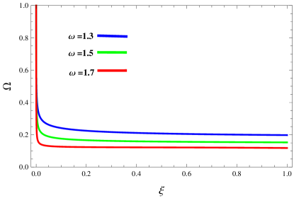
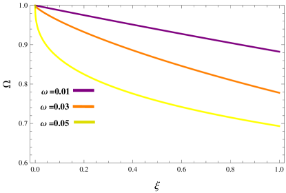
Figure 1: Plots of energy density versus $\xi$ for $n=3$, $\rho_{o}=5$, $\zeta=7$, $\beta=0.001$.

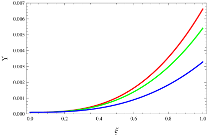
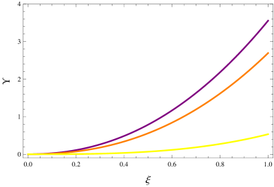
Figure 2: Plots of mass function versus $\xi$ for $n=3$, $\rho_{o}=5$, $\zeta=7$, $\beta=0.001$.

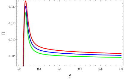
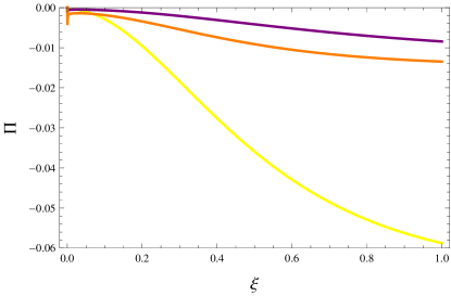
Figure 3: Plots of anisotropy versus $\xi$ for $n=3$, $\rho_{o}=5$, $\zeta=7$, $\beta=0.001$.

For graphical analysis, we choose $n=3,~{}\rho_{o}=5,~{}\zeta=7$ and $\beta=0.0010$. Figures 1-3 show the behavior of dimensionless energy density, mass function and anisotropy, respectively. It can be seen from Figure 1 that $\Omega$ is a decreasing function for smaller as well as greater values of $\omega$. Moreover, the mass function has an inverse relationship with $\omega$ while it varies directly with $\xi$. Further, we note an increment in the anisotropy as $\omega$ rises from 1.3 to 1.7. In contrast, the anisotropy within the system is negative when $\omega$ increases from 0.01 to 0.05. Thus, the physically acceptable solution is associated with $\omega=1.3,~{}1.5,~{}1.7$.

6 Conclusions

In this paper, we have studied the impact of charge on the complexity of a static sphere within the framework of EMSG. In this respect, we have constructed the EMSG fields equations for a static sphere by considering an anisotropic fluid distribution in the presence of electromagnetic field. We have formulated the mass functions m and $\emph{m}_{Tol}$ by utilizing the definitions given by Misner-Sharp and Tolman, respectively. Their link with Weyl tensor and matter variables has also been discussed. We have also formulated the TOV equation in the context of EMSG. The complexity factor has been obtained by formulating the structure scalars through the orthogonal decomposition of the curvature tensor. The scalar $\mathcal{Y}_{TF}$ accommodated the inhomogeneous energy density, charge, anisotropic pressure and dark source terms of $f(R,\textbf{T}^{2})$ gravity. Moreover, we have obtained the expression of Tolman mass in terms of this strucuture scalar in the presence of charge. Consequently, we have chosen $\mathcal{Y}_{TF}$ as a complexity factor. We have found that the addition of charge decreases the complexity of stellar structure.

We have formulated the disappearing complexity condition by setting $\mathcal{Y}_{TF}=0$. The vanishing complexity condition provides an extra constraint which assists in obtaining the solution of field equations by reducing the degrees of freedom. In this respect, we have determined the complexity factor for a specific model, $f\left(R,\textbf{T}^{2}\right)=R+\zeta\textbf{T}^{2}$. In GR, the self-gravitating spherical system has zero complexity if it is isotropic and homogeneous. However, in our work, an isotropic and homogeneous system does not correspond to zero complexity which implies the impact of dark source terms. Zero complexity is obtained for

$$\int^{r}_{0}\tilde{r}^{3}\left\{\left(\frac{1}{f_{R}}\right)^{{}^{\prime}}\left(\rho+\varphi+\varphi_{00}-\frac{\emph{q}^{2}}{8\pi r^{4}}\right)+\left(\frac{1}{f_{R}}\right)\Big{(}\varphi+\varphi_{00}-\frac{\emph{q}^{2}}{8\pi r^{4}}\Big{)}^{{}^{\prime}}\right\}\emph{d}\tilde{r}$$

$$+\frac{1}{f_{R}}\left(\frac{\left(\varphi_{22}-\varphi_{11}\right)}{2}+\frac{\emph{q}^{2}}{4\pi r^{4}}\right)=0.$$

Hence, the presence of additional matter terms of $f(R,\textbf{T}^{2})$ gravity has enhanced the complexity of stellar structure.

Finally, we have developed two solutions of EMSG field equations by assuming $\emph{q}(r)=\beta r^{3}$. Firstly, to investigate the features of stellar objects, we have assumed the energy density of compact structure suggested by Gokhroo and Mehra. Secondly, we have applied the polytropic equation of state and constructed a system of dimensionless equations by introducing some new variables. This system contained the dimensionless TOV equation, mass and disappearing complexity condition. We have graphically analyzed the numerical solution of this system by varying the parameter $\omega$. The system has positive energy density for smaller as well as larger values of $\omega$. However, the anisotropy corresponding to smaller values of $\omega$ is negative. Thus, we have concluded that the behavior of the considered system is physically acceptable for $\omega=1.3,~{}1.5,~{}1.7$. It is important to mention here that results of GR [5] can be retrieved corresponding to $\zeta=0$.

Data availability: No new data were generated or analyzed in support of this research.

References

[1] Kolmorgorov, A.N.: Prob. Inform. Theory J. 1(1965)3; Grassberger, P.: Int. J. Theor. Phys.
25(1986)907; Crutchfield, J.P. and Young, K.: Phys. Rev.
Lett. 63(1989)105; Anderson, P.W.: Phys. Today
44(1991)9; Parisi, G.: Phys. World 6(1993)42.
[2] Lopez-Ruiz, R., Mancini, H.L. and Calbet, X.: Phys. Lett. A
209(1995)321; Calbet, X. and Lopez-Ruiz, R.: Phys. Rev. E
63(2001)066116; Sañudo, J. and Lopez-Ruiz, R.: Phys.
Lett. A 372(2008)5283.
[3] Sañudo, J. and Pacheco, A.F.: Phys. Lett. A
373(2009)807; de Avellar, M.G.B. and Horvath, J.E.: Phys.
Lett. A 376(2012)1085; de Avellar, M.G.B. et al.: Phys.
Lett. A 378(2014)3481.
[4] Herrera, L.: Phys. Rev. D 97(2018)044010.
[5] Sharif, M. and Butt, I.I.: Eur. Phys. J. C 78(2018)850.
[6] Herrera, L., Di Prisco, A. and Ospino, J.: Phys. Rev. D 98(2018)104059.
[7] Herrera, L., Di Prisco, A. and Ospino, J.: Phys. Rev. D 99(2019)044049.
[8] Herrera, L., Di Prisco, A. and Ospino, J.: Eur. Phys. J. C 80(2020)631.
[9] Rosseland, S. and Eddington, A.S.: Mon. Not. R. Astron. Soc. 84(1924)720.
[10] Ray, S. et al.: Braz. J. Phys. 34(2004)310.
[11] Sharif, M. and Bhatti, M.Z.: Int. J. Mod. Phys. D 23(2014)1450085.
[12] Sharif, M. and Sadiq, S.: Eur. Phys. J. C 76(2016)568.
[13] Sharif, M. and Butt, I.I.: Eur. Phys. J. C 78(2018)688.
[14]Sharif, M. and Butt, I.I.: Chin. J. Phys. 61(2019)238.
[15] Riess, A.G. et al.: Astron. J. 116(1998)1009.
[16] Perlmutter, S. et al.: Astrophys. J. 517(1999)565.
[17] Tegmark, M. et al.: Phys. Rev. D 69(2004)103501; Seljak, U. et al.: Phys. Rev. D
71(2005)103515.
[18] Eisenstein, D.J. et al.: Astrophys. J. 633(2005)560.
[19] Anderson, L. et al.: Mon. Not. R. Astron. Soc. 427(2013)3435.
[20] Buchdahl, H.A.: Mon. Not. R. Astron. Soc. 1(1970)150.
[21] Harko, T. et al.: Phys. Rev. D 84(2011)024020.
[22] Harko, T. and Lobo, F.S.N.: Galaxies 2(2014)410.
[24] Abbas, G. and Nazar, H.: Eur. Phys. J. C 78(2018)510.
[25] Abbas, G. and Nazar, H.: Int. J. Geom. Methods Mod. Phys. 16(2019)1950174.
[26] Abbas, G. and Ahmad, R.: Astrophys. Space Sci. 364(2019)194.
[27] Sharif, M. and Majid, A.: Chin. J. Phys. 61(2019)38; Sharif, M., Majid, A. and Nasir, M.M.M.: Int.
J. Mod. Phys. A 34(2019)32; Yousaf, Z., Bhatti, M. and
Naseer, T.: Phys. Dark Universe 28(2020)100535.
[28] Astashenok, A.V. et al.: Phys. Lett. B 811(2020)135910; Astashenok, A.V. et al Eur. Phys. Lett. 134(2021)59001;
Astashenok, A.V. et al Eur. Phys. Lett. 136(2021)59001;
Oikonomou, V.K.: Class. Quantum Grav. 38(2021)175005.
[29] Katirci, N. and Kavuk, M.: Eur. Phys. J. Plus 129(2014)163.
[30] Roshan, M. and Shojai, F.: Phys. Rev. D 94(2016)4.
[31] Board, C.V.R. and Barrow, J.D.: Phys. Rev. D 96(2017)123517.
[32] Akarsu, Ö. et al.: Phys. Rev. D 97(2018)124017; Nari, N. and Roshan, M.: Phys.
Rev. D 98(2018)024031.
[33] Bahamonde, S., Marciu, M. and Rudra, P.: Phys. Rev. D 100(2019)083511.
[34] Sharif, M. and Gul, M.Z.: Phys. Scr. 96(2020)025002.
[35] Sharif, M. and Gul, M.Z.: Int. J. Mod. Phys. A 36(2021)2150004.
[36] Faraoni, V.: Phys. Rev. D 80(2009)124040.
[37] Zubair, M., Waheed, S. and Ahmad, Y.: Eur. Phys. J. C 76(2016)444.
[38] Misner, C.W. and Sharp, D.H.: Phys. Rev. 136(1964)B571.
[39] Tolman, R.: Phys. Rev. 35(1930)875.
[40] Bekenstein, J.D.: Phys. Rev. D 4(1971)2185.
[41] Herrera, L. et al.: Phys. Rev. D 79(2009)064025; Herrera, L., Di Prisco, A. and Ospino, J.:
Gen. Relativ. Gravit. 42(2010)1585.
[42] de Felice, F., Yu, Y. and Fang, Z.: Mon. Not. R. Aston. Soc. 277(1995)L17.
[43] Gokhroo, M.K. and Mehra, A.L.: Gen. Relativ. Gravit. 26(1994)75.
[44] Shapiro, S.L. and Teulolsky, S.A.: Black Holes, White Dwarfs and Neutron Stars (Johnwiley and Sons, 1983); Kippenhahn, R.
and Weigert, A.: Stellar Structure and Evolution
(Springer-Verlag, 1990).
[45] Herrera, L. et al.: Gen. Relativ. Gravit. 46(2014)1827.