Accelerating reactive-flow simulations using vectorized chemistry integration

Abstract

The high cost of chemistry integration is a significant computational bottleneck for realistic reactive-flow simulations using operator splitting. Here we present a methodology to accelerate the solution of the chemical kinetic ordinary differential equations using single-instruction, multiple-data vector processing on CPUs using the OpenCL framework. First, we compared several vectorized integration algorithms using chemical kinetic source terms and analytical Jacobians from the pyJac software against a widely used integration code, CVODEs. Next, we extended the OpenFOAM computational fluid dynamics library to incorporate the vectorized solvers, and we compared the accuracy of a fourth-order linearly implicit integrator–both in vectorized form and a corresponding method native to OpenFOAM—with the community standard chemical kinetics library Cantera. We then applied our methodology to a variety of chemical kinetic models, turbulent intensities, and simulation scales to examine a range of engineering and scientific scale problems, including (pseudo) steady-state as well as time-dependent Reynolds-averaged Navier–Stokes simulations of the Sandia flame D and the Volvo Flygmotor bluff-body stabilized, premixed flame. Subsequently, we compared the performance of the vectorized and native OpenFOAM integrators over the studied models and simulations and found that our vectorized approach performs up to $3335$$\times$ faster than the native OpenFOAM solver with high accuracy.

footnote

1 Introduction

Developers of next-generation combustion devices have increasingly turned to new operating regimes—e.g., low-temperature combustion [1]—to achieve higher efficiencies and reduced emissions. Computational reactive-flow modeling has been used to rapidly develop these new combustion concepts into functional prototypes [2], but accurately predicting combustion processes at these regimes depends on realistic chemical kinetics models. This places a large computational burden on reactive-flow modeling, since solving the ordinary differential equations (ODEs) governing chemical kinetics can dominate the overall cost of simulations. For example, in a study of n-dodecane spray injection, a high-resolution large-eddy simulation (LES) using a 54-species skeletal model and up to $22$ million cells took around $48,000$ CPU hours (or about 20 days of wall-clock time) to complete a single realization of just $2\text{\,}\mathrm{ms}\text{/}$ after start of injection [3]. Large model size and high numerical stiffness further increase computational cost, and unfortunately chemical kinetic models relevant to transportation or power-generation applications exhibit these characteristics [4].

Many strategies have been developed to reduce the cost of using realistic, detailed chemical kinetic models in reactive-flow simulations [4, 5]. Skeletal reduction methods aim to remove unimportant species and reactions from a chemical kinetic model while maintaining fidelity to the base detailed model [6, 7, 8, 9]. In addition, species with similar thermochemical properties may also be lumped together [10, 11, 12], time-scale methods can be used to reduce numerical stiffness [13, 14, 15, 16], and tabulation/interpolation methods reuse previously computed results to accelerate simulations [17, 18, 19]. Often, several of these techniques are combined to achieve better performance [20, 21, 22], or are even applied dynamically throughout a simulation to achieve greater local computational savings [23, 24, 25].

In addition to methods that reduce or approximate the base chemical kinetic model, performance can be increased by improving the ODE integration algorithms used to solve the chemical-kinetic equations. Some researchers have developed new integration algorithms specifically for efficiently solving chemical kinetics [26, 16, 27], while others have examined the performance of existing algorithms for use in reactive-flow simulations [28, 29, 30, 31, 32, 33]. Further, several codes have recently been developed for analytically evaluating the chemical-kinetic Jacobian matrix [34, 35, 36], which may be used to improve the performance of implicit ODE integration schemes [4].

In recent years, high-performance computing hardware has been evolving from a homogeneous, CPU-based paradigm to one dominated by heterogeneous processing architectures. In particular, single-instruction multiple-thread (SIMT) processors have become widely available, such as graphics processing units (GPUs), and many studies have leveraged their high floating-operation throughput to accelerate chemical-kinetics integration. Early work used GPUs to evaluate chemical-kinetic source terms or factorize the Jacobian matrix, but found significant speedups only for large chemical kinetic models [37, 38]. Later, several studies implemented GPU-based explicit integration techniques to achieve order-of-magnitude or more speedups when integrating non-stiff or moderately-stiff chemical kinetics [39, 28, 30]. Further work followed that developed GPU-based implicit integration schemes, but these exhibited decreased performance with increasing numerical stiffness due to thread divergence [40, 41, 42].

In contrast, vectorization based on the single-instruction multiple-data (SIMD) paradigm, like that found on modern CPUs, has not been as extensively investigated for use in chemical-kinetic integration, though SIMD vectorization has been used for ODE integration in related contexts [43, 44, 45]. Che et al. [46] used loop-unrolling/rearrangement, aligned arrays, and OpenMP [47] compilation directives (i.e., #pragmas) to achieve SIMD vectorization for accelerating an LES solver on the Intel Xeon Phi Many Integrated Core (MIC) co-processor. Stone et al. [33] used the OpenCL [48] framework to vectorize a linearly implicit Rosenbrock integration method [49] on the CPU, GPU, and MIC architectures. In addition, we developed the open-source platform pyJac that can generate vectorized, OpenCL-based chemical kinetic source term and Jacobian evaluation codes [35].

In this work, we describe a method to implement SIMD-based vectorized ODE integration methods—coupled with vectorized, analytical chemical kinetic Jacobian and source-term evaluations—for use in realistic reactive-flow simulations. Our primary focus is finding the acceleration and performance scaling achievable by the vectorized methods, so we examine these in applications with different turbulent and chemical time scales, mesh resolutions, and chemical-kinetic model sizes to assess their performance in a variety of engineering and scientific contexts. To do so, we extended the open-source computational fluid dynamics (CFD) code OpenFOAM [50] to use the vectorized methods.

Our goal here is to demonstrate the significant reduction in computational cost achievable by fully vectorized chemical-kinetic integration on CPUs without compromising accuracy, rather than to perform high-fidelity studies with the aim of investigating the combustion physics involved. Although the open-source nature of OpenFOAM is advantageous for these purposes—allowing modification to enable the vectorized ODE integration methods—it lacks some commonly used models (e.g., multi-component and mixture-averaged species transport [51]) and boundary conditions (e.g., Navier–Stokes Characteristic Boundary Conditions [52, 53]). It has to be pointed out that the impact of the interaction of errors from computational grid size, subgrid models, numerical schemes, and chemical kinetic model selection on the accuracy of reactive-flow simulations is not well understood. For instance, Cocks et al. [54] demonstrated that four different numerical schemes (as provided by industry, research, and open-source CFD codes) are unable to produce consistent reactive-flow LES solutions for the commonly used Volvo bluff-body stabilized flame [55, 56, 57], even when using the same computational grid, subgrid, and chemistry models. Similarly, Rochette et al. [58] found that the numerical scheme and chemical kinetic model have a large effect on the agreement of the solution with experimental data used in a reactive-flow LES solution of the Volvo bluff-body stabilized flame problem. The focus of this work is not model validation, so we will use only built-in OpenFOAM numerical schemes, subgrid models, and boundary conditions—substituting in our vectorized ODE solver—to simulate selected reactive-flow problems, demonstrating that the techniques developed here can further aid the development of standard models in OpenFOAM.

The rest of this article is organized as follows. Section 2 describes the numerical methods and software used in this study. Subsequently, Section 3 first verifies the vectorized solvers against a typical implicit integration algorithm, then confirms their coupling to the CFD code OpenFOAM [50]. Then, Section 4 presents two case studies that compare the performance of the vectorized solvers with those built into OpenFOAM: Sandia flame D [59, 60, 61] in Section 4.1 and the Volvo Flygmotor bluff-body flame [55, 56, 57] in Section 4.2. Finally, in Section 6 we identify and discuss directions for future efforts.

2 Numerical methods and software

2.1 pyJac code-generation platform

pyJac [35] is an open-source software package that generates code for evaluating the chemical-kinetic source terms and analytical Jacobian matrix for a variety of execution, data-ordering, and matrix-format patterns. For full details, we direct readers to our prior work focusing on pyJac [34, 35]; however, here we highlight key points relevant to this work. When using the constant-pressure assumption, the resulting thermochemical state vector in pyJac is

$$\Phi=\left\{T,V,n_{1},n_{2},\ldots,n_{N_{\text{sp}}-1}\right\}\;,$$ (1)

where $T$ is the temperature of the gas mixture, $V$ is the volume, $n_{i}$ is the moles of species $i$, and $N_{\text{sp}}$ is the number of species in the model. The last species in the model is typically the bath gas—N2 in this study—and omitted from the state vector, as it is calculated implicitly via the ideal gas equation of state:

$$n=\frac{PV}{\mathcal{R}T}=\sum_{i=1}^{N_{\text{sp}}}{n_{i}}\;,$$ (2)

where $n$ is the total number of moles of the gas mixture and $\mathcal{R}$ is the universal gas constant. The moles of the last species in the model $n_{N_{\text{sp}}}$ is then calculated as

$$n_{N_{\text{sp}}}=\frac{PV}{\mathcal{R}T}-\sum_{i=1}^{N_{\text{sp}}-1}{n_{i}}\;.$$ (3)

This formulation explicitly conserves mass in pyJac, and also ensures that the system of equations is not overconstrained [36].

Given a thermochemical state vector, pyJac can evaluate the chemical kinetic source rates

$$\frac{\text{d}\Phi}{\text{d}t}=f\left(\Phi\right)=\left\{\frac{\text{d}T}{\text{d}t},\frac{\text{d}V}{\text{d}t},\frac{\text{d}n_{1}}{\text{d}t},\frac{\text{d}n_{2}}{\text{d}t},\ldots,\frac{\text{d}n_{N_{\text{sp}}-1}}{\text{d}t}\right\}\;,$$ (4)

which form the autonomous chemical kinetic ODEs. In addition, pyJac can calculate the analytical chemical kinetic Jacobian

$$\mathcal{J}_{i,j}=\frac{\partial f_{i}}{\partial\Phi_{j}},\qquad i,j=1,\ldots,N_{\text{sp}}+1\;.$$ (5)

Although pyJac can evaluate the Jacobian in a sparse-matrix format (e.g., compressed row storage), we used a dense-matrix format to simplify implementing linear-algebra operations; extending this effort to use a sparse matrix is a goal for future studies. We used pyJac to generate an explicit “shallow”-vectorization, as described in Section 2.2, using a vector width of eight double-precision floating-point operations, and “C” (or row-major) data ordering.

2.2 OpenCL and vectorization

The parallel programming standard OpenCL [48] provides a common interface to execute vectorized code on a variety of different platforms (e.g., CPU, GPU, MIC). For a detailed overview of different vectorization patterns and their applications to different hardware platforms for integrating chemical kinetic ODEs, we refer the reader to past works [35, 42, 40, 62]. Here we will discuss only the so-called “shallow”-vectorization pattern for SIMD processors (e.g., CPUs) using OpenCL.

This method groups together the thermochemical state vectors of several chemical kinetic ODE systems:

$$\Phi_{\text{vec}}=\Bigl{\{} \left\{\Phi_{1,1},\Phi_{2,1},\ldots,\Phi_{N_{v},1}\right\},$$

$$\left\{\Phi_{1,2},\Phi_{2,2},\ldots,\Phi_{N_{v},2}\right\},\ldots,$$

$$\left\{\Phi_{1,N_{\text{sp}}+1},\Phi_{2,N_{\text{sp}}+1},\ldots,\Phi_{N_{v},N_{\text{sp}}+1}\right\}\Bigr{\}}\;,$$ (6)

where $N_{v}$ is the number of elements in the vector, also known as the vector width, and $\Phi_{j,i}$ is the $i$th component of the thermochemical state vector (Eq. 1) for the $j$th state.

These modified state vectors can be loaded into OpenCL vector data types, e.g., double8, allowing floating-point math operations to be performed concurrently over the vector (by specialized vector processors present on all modern CPUs), thus accelerating computations. The OpenCL runtime (e.g., as supplied by Intel [63]) then transforms the OpenCL code into vectorized operations using the vector-instruction set present on the device.

2.3 accelerInt ODE integration library

Efficiently and accurately integrating the autonomous chemical kinetic ODEs is critical to simulating reactive flows. Integration advances the source rates—described in Section 2.1—from an initial time $t_{i}$ to a final time $t_{f}$:

$$\frac{\text{d}\Phi}{\text{d}t}=f\left(\Phi\right),\quad t_{i}\leq t\leq t_{f}\;.$$ (7)

We have implemented several previously developed vectorized OpenCL-based ODE integration methods [33] in the accelerInt software library [42]: a fourth-order explicit Runge–Kutta method and several third- and fourth-order linearly implicit Rosenbrock methods [64, 65, 49]. Table 1 lists the OpenCL-based solvers available in accelerInt, as well as their orders, solver types, and references.

Solver name	Order	Solver type	Reference(s)	Short name
Rosenbrock	3	Linearly implicit	[64, 65]	ROS3
Rosenbrock	4	Linearly implicit	[49]	ROS4
RODAS	3	Linearly implicit	[64, 65]	RODAS3
RODAS	4	Linearly implicit	[49]	RODAS4
RKF45	4	Explicit	[66]	RKF45

Table 1: List of vectorized OpenCL integration methods incorporated into accelerInt.

Runge–Kutta methods include both implicit and explicit solvers, and are widely used to solve systems of stiff and non-stiff ODEs. A Runge–Kutta method with $s$ stages may be written as

$$\Phi\left(t_{n+1}\right)=\Phi\left(t_{n}\right)+\sum_{i=1}^{s}b_{i}\bm{k}_{i}\;,$$ (8)

where each stage is computed as

$$\bm{k}_{i}=h\,f\left(\Phi\left(t_{n}\right)+\sum_{j=1}^{s}a_{ij}\bm{k}_{j}\right)\;,$$ (9)

where $h$ is the time-step size, and $a_{ij}$ and $b_{i}$ are method coefficients that define the algorithm.

The explicit solver included in accelerInt is a five-stage, fourth-order-accurate embedded Runge–Kutta–Fehlberg method (RKF45) [66]. Explicit Runge–Kutta methods are obtained when the coefficient matrix $a_{ij}$ in Eq. 9 is strictly lower triangular (i.e., $a_{ii}=0$). While explicit integration methods are efficient for non-stiff problems, they are only conditionally stable and perform poorly for stiff problems where the step size $h$ is limited by stability concerns rather than the desired accuracy.

Implicit Runge–Kutta methods result from a fully populated coefficient matrix $a_{ij}$, resulting in a system of non-linear equations that are typically solved via Newton–Raphson iteration. This technique requires the repeated evaluation and factorization of the chemical-kinetic Jacobian matrix $\mathcal{J}$ (see Eq. 5). As such, implicit methods cost more per integration step, but their improved stability typically makes them more efficient for solving stiff ODEs. Implicit methods commonly reuse the Jacobian matrix (and its factorization) for multiple time steps to reduce the computational overhead.

Rosenbrock (ROS and RODAS) methods are more similar in structure to Runge–Kutta methods than to fully implicit techniques. They solve a linearized form of Eq. 8 and are therefore known as “linearly implicit” techniques. An $s$-stage Rosenbrock method is formulated as

$$\bm{k}_{i}=hf\left(\Phi\left(t_{n}\right)+\sum_{j=1}^{i-1}\alpha_{ij}\bm{k}_{j}\right)+h\mathcal{J}\sum_{j=1}^{i}\gamma_{ij}\bm{k}_{j},\quad i=1,\ldots,s$$ (10)

$$\Phi\left(t_{n+1}\right)=\Phi\left(t_{n}\right)+\sum_{i=1}^{s}b_{i}\bm{k}_{i}\;,$$ (11)

where $\alpha_{ij}$, $\gamma_{ij}$, and $b_{i}$ are the method parameters. Typically Rosenbrock methods are constructed with $\gamma_{11}=\ldots=\gamma_{ss}=\gamma$, a constant parameter, such that only one LU decomposition must be performed per time step [49].

To avoid solving a linear system and performing matrix-vector multiplication at each stage of the method [49, 67], Eq. 10 may be transformed:

$$\left(\frac{1}{h\gamma_{ii}}\bm{I}-\mathcal{J}\right)\bm{u}_{i}=f\left(\Phi\left(t_{n}\right)+\sum_{j=1}^{i-1}a_{ij}\bm{u}_{j}\right)+\sum_{j=1}^{i}\frac{c_{ij}}{h}\bm{u}_{j},\quad i=1,\ldots,s$$ (12)

$$\Phi\left(t_{n+1}\right)=\Phi\left(t_{n}\right)+\sum_{j=1}^{s}m_{j}\bm{u}_{j}\;,$$ (13)

where $\bm{\Gamma}=\left(\gamma_{ij}\right)$ is an intermediate matrix constructed from the $\gamma_{ij}$ values,

$$\bm{u}_{i} =\sum_{j=1}^{i}\gamma_{ij}\bm{k}_{j}\;,$$ (14)

$$a_{ij} =\alpha_{ij}\bm{\Gamma}^{-1}\;,$$ (15)

$$c_{ij} =\gamma\bm{I}-\bm{\Gamma}^{-1}\;,\text{ and}$$ (16)

$$m_{j} =b_{j}\bm{\Gamma}^{-1}\;.$$ (17)

Directly using the Jacobian matrix in Rosenbrock solvers avoids the need for Newton iteration, making these methods particularly well-suited for SIMD and SIMT vectorization due to the low levels of divergence between vector lanes/threads [29]. However, ROS solvers are formulated around using an exact (analytical) Jacobian, since a finite-difference Jacobian may impact the solver’s order and convergence [49, 68]. Further, the Jacobian must now be evaluated/factorized at each step, adding to the cost per time step. W-methods may be a suitable technique to avoid these costs, since they are formulated around using an inexact Jacobian [49]; these should be investigated for vectorized ODE integration in the future.

These Runge–Kutta and Rosenbrock solvers, coupled with OpenCL source-rate/Jacobian evaluation code generated by the latest version of pyJac [35], form the basis of the accelerated ODE integration techniques used here.

2.4 OpenFOAM

OpenFOAM [50] is an open-source C++ library capable of solving a variety of continuum mechanics problems, and is designed to allow straightforward extension and implementation of custom solvers. In this work, we extend the OpenFOAM applications for solving reactive-flow CFD problems to incorporate the vectorized ODE integration techniques outlined in Section 2.3. The reactive-flow solver reactingFoam supports using a variety of boundary conditions, models, solution techniques, and turbulence descriptions, including Reynolds-averaged Navier–Stokes (RANS) and LES simulations. For comprehensive details on these models and their implementation in OpenFOAM we refer readers to dedicated articles on these topics [69, 70, 50, 71]. Here we focus on the models relevant to incorporating accelerInt into OpenFOAM for solving chemical kinetic ODEs.

2.4.1 Chemistry solvers

OpenFOAM has a number of built-in solvers for integrating the chemical kinetic ODEs, including C++ implementations of the third- and fourth-order linearly implicit Rosenbrock solvers in accelerInt. However, the implementations differ in a number of key aspects. First, and most obviously, the difference in programming languages results in different execution patterns: serial evaluation in OpenFOAM vs. vectorized/batched integration in accelerInt. Second, the ROS4 solver in OpenFOAM uses a different set of method coefficients [68] than those used in accelerInt [49]. Third, OpenFOAM v6.x includes an analytical Jacobian evaluation code, but it uses a different state vector composed of the species concentrations, temperature, and pressure (which is assumed constant, as in pyJac). Finally, OpenFOAM does not employ the explicit mass-conservation formulation employed by pyJac, i.e., the concentration of the last species in the model is solved for directly in OpenFOAM.

We created a new chemistry model for OpenFOAM by extending the base class BasicChemistryModel: BatchedChemistryModel. This new model performs the chemical-kinetic integration of the thermochemical state vectors for the domain (or sub-domain, in the case of runs parallelized with the message passing interface, MPI [72]) in a single batched call to the accelerInt library, instead of evaluating them sequentially as in the base OpenFOAM code. The accelerInt library returns the updated thermochemical state vectors for the domain, as well as the final internal integration time step taken for each cell in the domain. The time-step values are used as an initial time step for the next ODE integration of this cell (as in the BasicChemistryModel used in the OpenFOAM code), as well as to adaptively limit the overall CFD time-step size for certain OpenFOAM solvers (e.g., chemFoam).

2.4.2 Turbulent combustion model

OpenFOAM implements multiple turbulent combustion models for simulating turbulence-chemistry interactions in reactive-flow simulations, ranging from a simple infinitely fast chemistry model to the more-complex flame surface density formulation [73]. We selected the eddy-dissipation concept (EDC) [74] as a robust and relatively computationally expensive combustion model to demonstrate the performance of the vectorized ODE solvers. EDC is a commonly used technique for modeling turbulence-chemistry interaction, and has been applied to a large variety of combustion problems [75, 76, 77]. Conceptually, EDC is based upon the idea of the turbulent energy cascade [74] and involves both a fine-scale reactor and its non-reacting surroundings [75]. EDC models molecular mixing between the fine scales and their surroundings by mass transfer between the two. When using a detailed chemical kinetic model, the fine-scale reactor is typically treated as a perfectly stirred reactor and solved to equilibrium, imposing significant computational overhead [78].

The mean reaction rate for species $i$ in the EDC model [74, 75], $\overline{R}_{i}$, is given by

$$\overline{R}_{i}=\frac{\overline{\rho}}{\tau^{*}}\frac{\gamma_{L}^{2}\chi}{1-\gamma_{L}^{2}\chi}\left(\overline{Y}_{i}-Y_{i}^{*}\right)\;,$$ (18)

where $\overline{\rho}$ is the mean fluid density; $\overline{Y}_{i}$ and $Y_{i}^{*}$ are the fluid mean and fine-structure mass fractions of species $i$, respectively; $\tau^{*}$ and $\gamma_{L}$ are the fine-structure residence time and dimensionless length fraction, respectively; and $\chi$ is the fraction of fine-structure regions that interact with the rest of the fluid, typically assumed to be unity [75].

By definition, for the concentration of species $i$ we have

$$[C_{i}] =\rho\frac{Y_{i}}{W_{i}}=\frac{n_{i}}{V}\;,$$

and

$$\rho Y_{i} =W_{i}\frac{n_{i}}{V}\;,$$ (19)

where $W_{i}$ is the molecular weight of species $i$ and the volume $V$ is that of the corresponding CFD cell. Combining Section 2.4.2 with Eq. 18 gives the mean reaction rate in terms of species moles (the species state variable used in pyJac):

$$\overline{R}_{i}=\frac{1}{\tau^{*}}\frac{\gamma_{L}^{2}\chi}{1-\gamma_{L}^{2}\chi}\frac{W_{i}}{\overline{V}}\left(\overline{n}_{i}-n_{i}^{*}\right)\;.$$ (20)

where $\overline{n}_{i}$ and $n_{i}^{*}$ are the mean and fine-structure moles of species $i$, respectively. Both $\overline{n}_{N_{\text{sp}}}$ and $n_{N_{\text{sp}}}^{*}$, the numbers of moles of the last species in the model in the mean and fine structures, respectively, are calculated using Eq. 3 to be consistent with pyJac.

3 Verification

In this section, we will verify the accuracy of the vectorized ODE solvers in two contexts. First, we will directly compare the vectorized solvers implemented in accelerInt against the commonly used high-order implicit solver CVODEs [79, 80, 81], to verify their accuracy and examine their relative performance. Then, we will compare the accuracy of the vectorized ROS4 solver coupled to OpenFOAM (using the methods described in Section 2.4) and the same ROS4 solver natively implemented in OpenFOAM to a reference chemical kinetics code Cantera [82] for constant-pressure homogeneous ignition problems.

3.1 accelerInt verification

To verify the new solvers, we sampled $100,000$ thermochemical conditions from a previously generated database [83], created using constant-pressure partially stirred reactor simulations [34] with the GRI-Mech 3.0 [84] chemical kinetic model, which consists of $53$ species and $325$ reactions. The database covers a pressure range of $125\text{\,}\mathrm{atm}\text{/}$ and a range of temperatures and compositions from a cold unburned CH4/air mixture to states of ignition and equilibrium. These conditions were integrated using CVODEs [79, 80, 81] with tight integration tolerances (absolute tolerance of ${10}^{-20}$, relative tolerance of ${10}^{-15}$) for a single global time step of ${10}^{-6}\text{\,}\sec$ to form a reference solution.

We then used the OpenCL solvers to integrate the same initial values to the same end time, varying the tolerances given to the adaptive time-stepping algorithm over ${10}^{-4}$, ${10}^{-5}$, …, ${10}^{-15}$. We set both the relative and absolute tolerances for the OpenCL solvers to this tolerance value for the verification effort; in general these can be (and often are) different, e.g., as in the computation of the reference CVODEs solution.

The error of each initial value problem (IVP) was then measured as

$$\lVert E_{j}\rVert=\left\lVert\frac{\lvert y_{i,j}^{\circ}(t)-y_{i,j}(t)\rvert}{${10}^{-10}$+${10}^{-6}$\times\lvert y_{i,j}^{\circ}(t)\rvert}\right\rVert_{2}\;,$$ (21)

where $y_{i,j}^{\circ}(t)$ is the $i$th component of the solution computed by CVODEs for the $j$th IVP and $y_{i,j}(t)$ is the solution computed by the solver being tested. The “tolerances” used for calculating the weighted reference solution components in Eq. 21 are for normalization purposes only, and are selected solely because they are the tolerances that will be used for the reactive-flow test-case (Section 4.2.2). The error over all IVPs was then calculated using the infinity norm

$$\lVert E\rVert=\lVert E_{j}\rVert_{\infty}=\max_{j}|E_{j}|\;.$$ (22)

The tested solvers used the same vectorization settings described in Section 2.1. Figure 1 shows the work-precision diagram for the accelerInt solvers: the vertical axis shows the error (as measured by Eqs. 21 and 22) for the solvers over the various tolerances tested, while the horizontal axis shows the mean CPU runtime (averaged over five individual runs) on a single core of an Intel® Xeon® X5650 CPU (with SSE4.2 vector instructions), using v16.1.1 of the Intel OpenCL runtime [63]. We omitted RKF45 from this test, as the stiffness of the chemical kinetic ODEs caused prohibitive computational costs; this solver will be examined in future work for less-stiff problems.

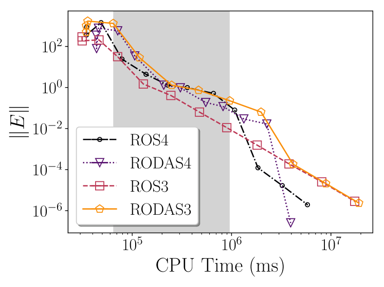
Figure 1: Work-precision diagram for the implicit OpenCL solvers in accelerInt. The vertical axis shows the error norm computed by Eqs. 21 and 22, while the horizontal axis shows the mean runtime of the solver, measured in $\mathrm{ms}\text{/}$. The region marked in grey corresponds to “intermediate” tolerances, ranging from ${10}^{-7}{10}^{-11}$ (with equal absolute and relative tolerances in the adaptive time-stepping algorithm).

For loose tolerances (${10}^{-4}{10}^{-6}$), the tested solvers all exhibit similar performance and error. However, for intermediate tolerances (${10}^{-7}{10}^{-11}$, marked in grey on Fig. 1) the ROS3 solver consistently has the lowest error compared with the reference solution; the fourth-order solvers (ROS4, RODAS4) tend to be slightly faster for a minor increase in error in this region. The higher accuracy of the ROS3 solver in this region is likely due to using a different set of method coefficients (see Table 1). At strict tolerances, i.e., less than ${10}^{-11}$, the ROS4 solver is both faster and more accurate than the third-order methods, while the RODAS4 solver is the most accurate for the strictest tolerance of ${10}^{-15}$.

3.2 Constant-pressure ignition in OpenFOAM

To verify the coupling of the accelerInt solvers to the OpenFOAM chemistry model (see Section 2.4), we ran a series of constant-pressure homogeneous ignition problems over initial temperatures of $T_{0}=$ $85011001500\text{\,}\mathrm{K}\text{/}$, initial pressures of $P_{0}=$ $11025\text{\,}\mathrm{atm}\text{/}$, and equivalence ratios of $\phi=$ $0.51.01.5$ in air, using the GRI-Mech 3.0 chemical kinetic model [84] and CH4 as the fuel. These conditions cover low-, intermediate-, and high-temperature ignition, as well as lean, stoichiometric, and rich fuel-air mixtures to test the accuracy of the solvers over different chemical kinetic regimes. To test the relative accuracy of the various solvers, the ignition problems were simulated to near chemical equilibrium (post-ignition) with both accelerInt and the built-in OpenFOAM integrators. The values of the thermochemical-state vectors for each solver were sampled $10$ times, equally distributed over the entire simulated time span (excluding the initial state); Fig. 2(a) shows an example of the time sampling. We compared the sampled values of both approaches with a reference solution computed using the open-source, community chemical kinetics code Cantera [82]. In this example we used the fourth-order linearly implicit Rosenbrock solver (ROS4) in both OpenFOAM and accelerInt, and set the absolute and relative integration tolerances to ${10}^{-10}$ and ${10}^{-6}$, respectively, for the OpenFOAM and accelerInt solvers, and to ${10}^{-20}$ and ${10}^{-15}$ for Cantera.

Figure 2 compares the values of the temperature and species mass fractions of CH4, OH, and NO for several initial conditions, showing that all three solvers agree qualitatively. To quantify this comparison, the supremum and mean $L^{2}$ norms of the (filtered) relative error between the tested solvers and Cantera were calculated respectively as

$$\lVert E\rVert_{\infty} =\left\lVert\frac{\lvert\Phi^{\circ}_{i}\left(t_{j}\right)-\Phi_{i}\left(t_{j}\right)\rvert}{\lvert$1\text{\times}{10}^{-10}$+\Phi_{i}^{\circ}\left(t_{j}\right)\rvert}\right\rVert_{\infty}$$ (23)

$$\lVert E\rVert_{\text{mean}} =\frac{1}{N_{s}\left(N_{\text{sp}}+1\right)}\left\lVert\frac{\lvert\Phi^{\circ}_{i}\left(t_{j}\right)-\Phi_{i}\left(t_{j}\right)\rvert}{\lvert$1\text{\times}{10}^{-10}$+\Phi_{i}^{\circ}\left(t_{j}\right)\rvert}\right\rVert_{2}\;,$$ (24)

where $N_{s}$ is the total number of sampled points, $N_{\text{sp}}+1$ is the size of the thermochemical state vector used in OpenFOAM (i.e., the temperature and all species concentrations), $\Phi_{i}\left(t_{j}\right)$ is the $i$th entry of the state vector calculated by either the built-in OpenFOAM or coupled accelerInt ROS4 solver at the $j$th sampled point, and $\Phi^{\circ}_{i}\left(t_{j}\right)$ the reference value calculated by Cantera.

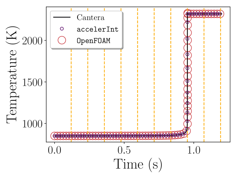
(a) The predicted temperature traces at $P_{0}=$25\text{\,}\mathrm{atm}\text{/}$$, $T_{0}=$850\text{\,}\mathrm{K}\text{/}$$, and CH4/air of $\phi=1.5$. The vertical dashed lines show the points at which the solution was sampled for error evaluation.

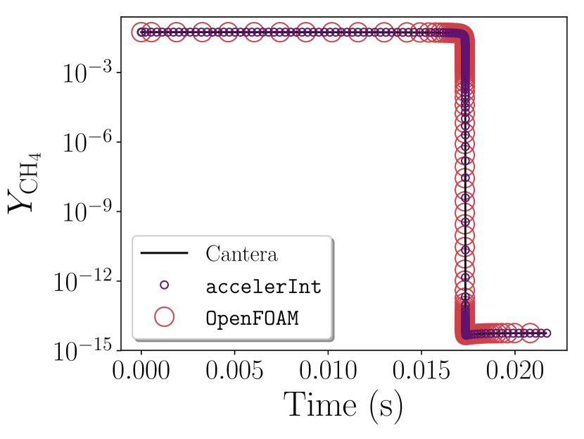
(b) The CH4 mass-fraction profiles predicted by the various solvers at $P_{0}=$10\text{\,}\mathrm{atm}\text{/}$$, $T_{0}=$1100\text{\,}\mathrm{K}\text{/}$$, and CH4/air of $\phi=1.0$

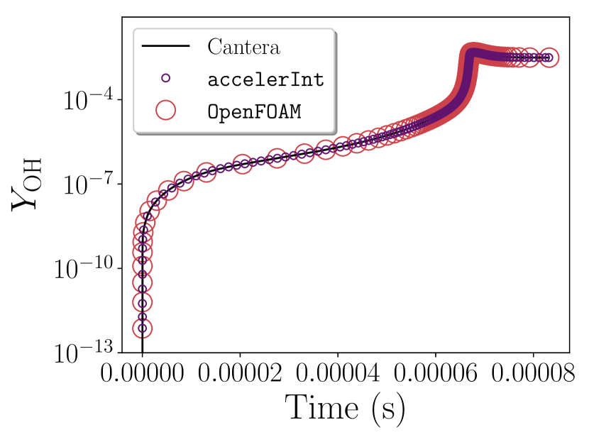
(c) The OH mass-fraction profiles predicted by the various solvers at $P_{0}=$25\text{\,}\mathrm{atm}\text{/}$$, $T_{0}=$1500\text{\,}\mathrm{K}\text{/}$$, and CH4/air of $\phi=0.5$

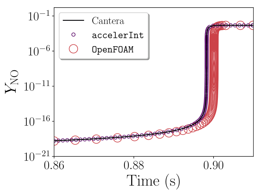
(d) A zoomed-in look at the NO mass-fraction profiles predicted by the various solvers during the ignition event, for $P_{0}=$25\text{\,}\mathrm{atm}\text{/}$$, $T_{0}=$850\text{\,}\mathrm{K}\text{/}$$, and CH4/air of $\phi=1.0$.

Figure 2: Comparison of constant-pressure homogeneous ignition problem with various solvers using GRI-Mech 3.0. The plotted points for the built-in OpenFOAM and coupled accelerInt ROS4 solvers were thinned somewhat for visibility.

Table 2 shows the values of these norms for both solvers; the coupled accelerInt solver agrees much better with the reference solution computed by Cantera than the built-in OpenFOAM solver. Although the computed error norms for OpenFOAM are several orders of magnitudes larger (i.e., $\mathcal{O}\left(10^{5}\right)$–$\mathcal{O}\left(10^{6}\right)$ versus $\mathcal{O}\left(10^{-1}\right)$–$\mathcal{O}\left(1\right)$ for accelerInt), this does not imply that the built-in OpenFOAM ROS4 solver is grossly inaccurate; indeed, a visual comparison of the solutions over the entire simulation (Figs. 2(b), 2(c) and 2(a)) show no easily discernible discrepancies. Instead, this difference largely results from more-accurate predictions of ignition delay time on the part of accelerInt. For instance, Fig. 2(d) shows the predicted mass fraction of NO during ignition for the stoichiometric case with an initial pressure of $25\text{\,}\mathrm{atm}\text{/}$ and temperature of $850\text{\,}\mathrm{K}\text{/}$. The OpenFOAM solver predicts ignition about $1.8\text{\,}\mathrm{ms}\text{/}$ later than either accelerInt or Cantera, a mere difference. Nonetheless, we conclude that the coupled accelerInt ROS4 solver is more accurate than the corresponding built-in OpenFOAM implementation.

Solver	$\lVert E\rVert_{\text{mean}}$	$\lVert E\rVert_{\infty}$
OpenFOAM	$4.68\text{\times}{10}^{5}$	$9.49\text{\times}{10}^{6}$
accelerInt	$3.39\text{\times}{10}^{-1}$	$8.12$

Table 2: The filtered mean and supremum relative error norms comparing the computed solutions of the built-in OpenFOAM and coupled accelerInt ROS4 solvers to those of Cantera for the homogeneous constant-pressure ignition problems.

4 Case studies

After verifying the accuracy of the accelerInt solvers, we next compare the performance of the built-in OpenFOAM and accelerInt ROS4 solvers on realistic reactive-flow simulations: the Sandia flame D and the Volvo Flygmotor bluff-body stabilized flame. Our objective in both cases is to determine the potential speedup offered by the vectorized solver.

4.1 Sandia flame D

The Sandia Flame D [59, 60, 61] is a well-characterized piloted CH4/air jet flame with a turbulent Reynolds number of $\text{Re}_{t}=22000$. OpenFOAM v5.x (the 2017 release from the OpenFOAM foundation [85]) and later include a case modeling this flame as a tutorial, providing a relatively inexpensive but more-realistic proving ground for the coupled accelerInt solvers. Table 3 and Table 4 list the operating conditions and key dimensions of the case, and Fig. 3(c) shows a schematic of the configuration superimposed over the simulation mesh.

	Source
	Jet	Coflow	Pilot
Composition	CH4/Air: 25/$75\text{\,}\mathrm{\char 37\relax}\text{/}$†	Dry air	Equil.‡
Velocity	$49.6\text{\,}\mathrm{m}\text{/}\mathrm{s}$	$0.9\text{\,}\mathrm{m}\text{/}\mathrm{s}$	$11.4\text{\,}\mathrm{m}\text{/}\mathrm{s}$
Temperature	$294\text{\,}\mathrm{K}\text{/}$	$291\text{\,}\mathrm{K}\text{/}$	$1880\text{\,}\mathrm{K}\text{/}$
Pressure	$0.993\text{\,}\mathrm{atm}\text{/}$	$0.993\text{\,}\mathrm{atm}\text{/}$	$0.993\text{\,}\mathrm{atm}\text{/}$

Table 3: Operating conditions for the Sandia Flame D case.

• The jet composition is measured by percent volume.

• Equilibrium state of CH4/air at $\phi=0.7$.

Dimension	Value
$D_{\text{jet, inner}}$	$7.2\text{\,}\mathrm{mm}\text{/}$
$D_{\text{pilot, inner}}$	$7.7\text{\,}\mathrm{mm}\text{/}$
$D_{\text{pilot, outer}}$	$18.2\text{\,}\mathrm{mm}\text{/}$
$D_{\text{wall, outer}}$	$18.9\text{\,}\mathrm{mm}\text{/}$
Exit	$30\text{\,}\mathrm{mm}\text{/}$ $\times$ $30\text{\,}\mathrm{mm}\text{/}$

Table 4: Diameter of the jet, pilot, and wall, and exit-plane dimensions for the Sandia Flame D case.

The mesh for this case, pictured in Fig. 3(a), is fully orthogonal with $5170$ cells, ranging in size from roughly $5\text{\,}\mathrm{mm}\text{/}$ on a side to $0.72\text{\,}\mathrm{mm}\text{/}$ tall near the wall. The solution domain is a thin three-dimensional wedge, with axi-symmetric boundary conditions on the front and back faces, and zero-gradient/total-pressure boundary conditions on the outlet. The case, as packaged with OpenFOAM, uses second-order interpolation and gradient schemes for all variables, but a strongly limited scheme (tending towards first-order) for divergence calculations. In addition, the simulation uses a standard $k$–$\varepsilon$ RANS model to model turbulence and a pseudo-transient, first-order time-stepping scheme to initially advance to a steady-state solution.

We modified the baseline case slightly to better suit the purposes of this study. First, we substituted the full GRI-Mech 3.0 chemical kinetic model [84] for the 36-species skeletal methane model originally used in OpenFOAM. Second, the base OpenFOAM case uses a tabulated dynamic adaptive chemistry scheme [19, 18] to accelerate the solution process; we disabled this to directly compare the performance and accuracy of the ODE solvers. Finally, after reaching steady state, we switched the time-stepping scheme to the second-order implicit method, set the minimum reacting temperature to $500\text{\,}\mathrm{K}\text{/}$, and ran the case for an additional $10\text{\,}\mathrm{ms}\text{/}$ of simulated time using a CFD time step of $\Delta t=${10}^{-6}\text{\,}\sec$$.

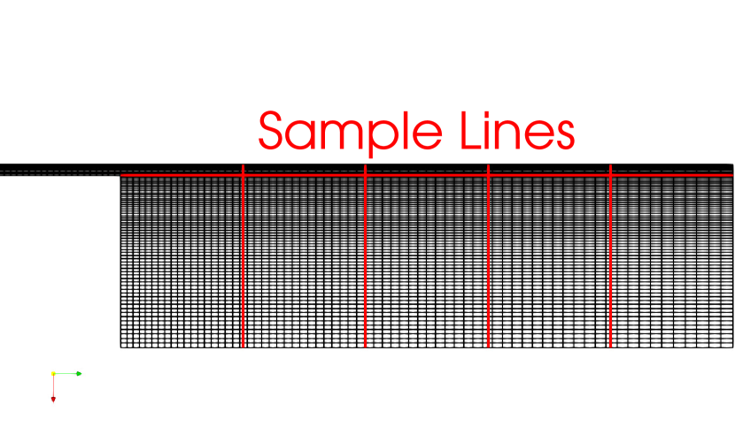
(a) The mesh for the Sandia Flame D case. The red line denotes where we sampled the solution for validation.

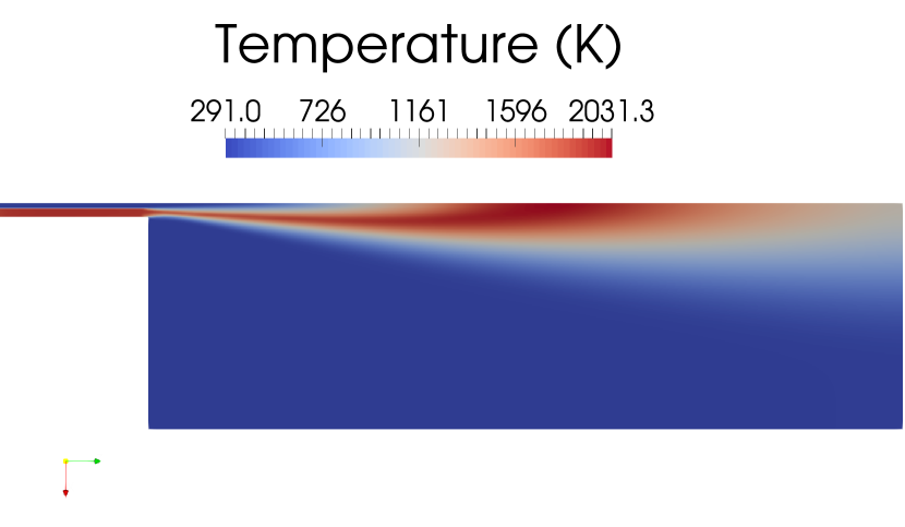
(b) The steady-state temperature profile in $\mathrm{K}\text{/}$, as solved by the base OpenFOAM fourth-order Rosenbrock ODE integrator.

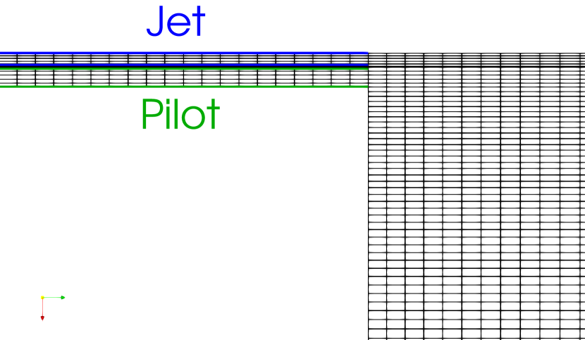
(c) A close-up view of the inlet to the domain. The jet and pilot flames are marked in blue and green, respectively. The sample lines are marked in red, as in Fig. 3(a)

Figure 3: The mesh and steady-state temperature profile of the Sandia Flame D case.

Using this case, we tested the performance of the various OpenFOAM and accelerInt solvers. Our goal here is to demonstrate the performance enhancement achievable through vectorized chemical kinetic integration, using available Intel CPUs; though dated, the AVX2 instruction set remains broadly relevant for CPUs that do not support the newer AVX-512 set. We ran the performance studies on $10$ cores of an Intel E5-2690 V3 CPU, with AVX2 vector instructions, $128\text{\,}\mathrm{Gbit}\text{/}$ of RAM, and v16.1.1 of the Intel OpenCL runtime. We used OpenFOAM version 6.x with v2.1.0 of the OpenMPI library [86], compiled with gcc v5.4.0 [87]. We instrumented the reactingFoam solver with the MPI profiling library IPM v2.0.6 [88] by placing profiling sections (via MPI_PControl) around the calls to the turbulent combustion model, ODE integration, and other key parts of the CFD time step (e.g., convection evaluation). Section S1 of the Supplemental Material compares in detail the predicted results for the different solvers; here, we focus on the computational cost/performance.

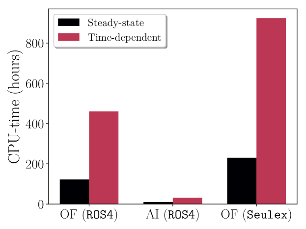
Figure 4: Total CPU hours spent evaluating chemistry in the Sandia Flame D case. AI is accelerInt and OF is OpenFOAM.

Figure 4 shows the total wall-clock execution time (over all $10$ processors) spent by each solver integrating the chemical kinetic ODEs. The accelerInt solver spends just 10.2 and $31.1\text{\,}\mathrm{h}\text{/}$ solving chemistry for the steady-state and time-dependent cases, respectively, while both the OpenFOAM solvers take over $100\text{\,}\mathrm{h}\text{/}$ in all cases. The slowest integration method is the OpenFOAM Seulex solver, which takes over $923\text{\,}\mathrm{h}\text{/}$ to complete the time-dependent solution. The chemistry evaluation time includes time spent idle due to the poor load balancing of chemistry present in most OpenFOAM simulations.

	Solver
	AI (ROS4)	OF (ROS4)	OF (Seulex)
Steady-state	$12.0\text{\,}\times$	–	$0.53\text{\,}\times$
Time-dependent	$14.8\text{\,}\times$	–	$0.50\text{\,}\times$
Chemistry time

Table 5: Speedups of the chemistry solvers (AI is accelerInt and OF is OpenFOAM), normalized by the OpenFOAM ROS4 solver and the percent of total execution time spent integrating the chemical-kinetic ODEs.

Table 5 compares the speedups of the solvers, reported against the OpenFOAM ROS4 solver as the baseline. The accelerInt ROS4 solver performs $12.014.8$$\times$ faster than the OpenFOAM equivalent. In addition, the OpenFOAM Seulex solver runs roughly 2$\times$ slower than the OpenFOAM ROS4 solver in both cases. Finally, the accelerInt solver spends in chemistry integration, while both OpenFOAM methods use over of the runtime solving chemistry.

4.2 Volvo bluff-body stabilized flame

Next, we will use the Volvo Flygmotor bluff-body stabilized premixed flame experiment [55, 56, 57] as a second test case. We simulated a reacting case, and used this to study the speedup of the coupled accelerInt solver compared to the built-in OpenFOAM method.

4.2.1 Case description

The Volvo Flygmotor bluff-body stabilized premixed flame experiments include many phenomena found in practical combustors, such as anchored flames, recirculation regions, and shear layers [55, 56, 57]. The computational domain is relatively simple and inexpensive to simulate, though, and it is a well-studied test case for non-swirling turbulent flames [89, 90, 91, 92, 54, 58]. Furthermore, experimental velocity, turbulence statistics, and temperature measurements are available for two inlet velocities and temperatures for validation purposes [55, 56, 57]. Section S2 of the Supplemental Material contains a validation of our setup using the non-reacting simulated velocity and turbulence statistics, compared with available experimental data; we did not include this in the main text, since our main focus is computational performance of the reacting solver.

Figure 5(a) shows the computational domain we used here, which omits the fuel injection, seeding, and flow-straightener parts upstream of the bluff body. Instead, we set steady inflow boundary conditions at $$5$D$—where $D=$40\text{\,}\mathrm{mm}\text{/}$$ is the bluff-body height—upstream of the trailing edge of the bluff body, as used in previous studies [90, 93, 54]. The domain extends $0.662\text{\,}\mathrm{m}\text{/}$ downstream of the trailing edge of the bluff body, where we used wave-transmissive outflow conditions as suggested in previous work [93, 90, 92]. The domain is $$2$D$ wide in the span-wise direction; the front and back faces of the domain use periodic boundary conditions to reduce computational effort [93, 54]. The walls of the domain use adiabatic and no-slip boundary conditions. Table 6 lists the inlet conditions, based on the available experimental conditions [94].

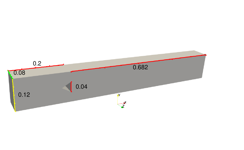
(a) Schematic of the computational domain for the Volvo bluff-body stabilized flame case. All distances are in meters.

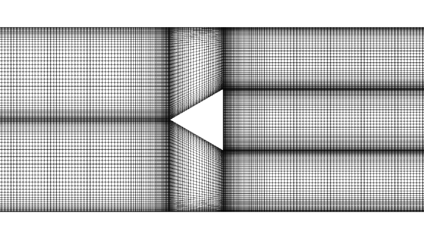
(b) A close up of the computational mesh near the bluff body. The cells are gradually stretched from a maximum wall-normal distance of $0.3\text{\,}\mathrm{mm}\text{/}$ near the walls and bluff body to a nominal mesh size of $2\text{\,}\mathrm{mm}\text{/}$.

Figure 5: The computational (a) domain and (b) mesh for the Volvo bluff-body stabilized flame case.

We developed the computational mesh (shown in Fig. 5(b)) based on recommendations from previous studies [54, 93]; it uses hexagonal cells nominally $2\text{\,}\mathrm{mm}\text{/}$ large and a maximum wall-normal distance of $0.3\text{\,}\mathrm{mm}\text{/}$. Grading clusters the cells near the walls and bluff-body edges, as well as the shear layers downstream of the bluff body; the domain is as isotropic as possible elsewhere, resulting in a total of $2,365,000$ mesh cells.

Parameter	Non-reactive	Reactive
Pressure	$1\text{\,}\mathrm{bar}\text{/}$	$1\text{\,}\mathrm{bar}\text{/}$
Temperature	$288\text{\,}\mathrm{K}\text{/}$	$288\text{\,}\mathrm{K}\text{/}$
$U_{\text{bulk}}$	$16.6\text{\,}\mathrm{m}\text{/}\mathrm{s}$	$17.3\text{\,}\mathrm{m}\text{/}\mathrm{s}$

Table 6: Inlet conditions for non-reactive and reactive cases [93], selected to match the available archived experiment data [94]. $U_{\text{bulk}}$ is the bulk inlet velocity.

To simulate this case we used the OpenFOAM solver reactingFoam with the LES turbulence model, along with a Smagorinsky subgrid scale model [95]. A second-order accurate central-differencing scheme discretized the Laplacian terms, while the solver used a second-order bounded cell-based Green-gauss method for gradient calculations. We used a second-order weakly-limited central scheme to calculate the velocity advection divergence and strong limiting for turbulent kinetic energy, species, and energy scalars. The solver advanced in time with a blended first- and second-order Crank–Nicolson scheme, and we handled pressure-velocity coupling with the PISO (pressure-implicit with split operator) algorithm [96]. Using a fully implicit second-order time-stepping method (along with an unlimited velocity advection scheme) was possible with multiple outer corrector steps—i.e., the PIMPLE algorithm in place of PISO—to avoid breakup of the flow due to pressure-velocity decoupling. However, this would require multiple solutions of the chemical kinetic ODEs at each step of the simulation, and consequentially make completing a single time step using the OpenFOAM ODE solvers take longer than the largest available time reservation on the computing cluster we used here. Hence, we used the blended time stepping and weakly limited velocity advection schemes instead.

4.2.2 Results

We ran the performance studies on 96 cores (i.e., four nodes with 2$\times$12 cores on each) of an Intel E5-2690 V3 CPU, with AVX2 vector instructions, $128\text{\,}\mathrm{GB}\text{/}$ of RAM, and using the Intel OpenCL runtime v16.1.1. We used OpenFOAM version 6.x [97] with v2.1.0 of the OpenMPI library [86], compiled with gcc v5.4.0 [87]. We instrumented the reactingFoam solver with the MPI-profiling library IPM v2.0.6 [88] by placing profiling sections (via MPI_PControl calls) around the calls to the turbulent combustion model, ODE integration, and other key parts of the CFD time step (e.g., convection evaluation). The absolute and relative tolerances of the OpenFOAM and accelerInt ROS4 solvers were ${10}^{-10}$ and ${10}^{-6}$, respectively.

Although the Volvo bluff-body reactive flame experiments used a lean propane-air mixture (overall global equivalence ratio of $\phi=$0.6$$), here we chose a stoichiometric CH4/air combustion case for this study. Previous studies have shown mixed agreement between simulated and experimental results using OpenFOAM on this configuration [54, 92]. Considering the many potential sources of error in a reactive-flow simulation [58]—e.g., the quality of chemical kinetic model, the turbulence-chemistry interaction model, and the numerical solver itself [54]—we opted to focus on the performance of the ODE integration algorithms instead of a detailed comparison of the reactive-flow case to the experimental data (as done for the non-reactive case as shown in the Supplemental Material). While we expect that these results could be reproduced for, e.g., the UCSD propane model [98] with $57$ species and $268$ reactions, we prefer to simply use the comparably sized GRI-Mech 3.0 [84] for our demonstration.

We initialized the reactive-flow case using a RANS simulation with the coarse ($4\text{\,}\mathrm{mm}\text{/}$ nominal cell size) mesh and the base OpenFOAM ROS4 integrator. A two-step methane model [99] ignited the flame via a spherical high-temperature kernel placed behind the bluff body. After the flame stabilized and attached to the bluff body, we ran the RANS simulation using the two-step methane model for a single flow-through time to develop the temperature field. Next, we mapped the RANS solution onto the same coarse mesh using the full GRI-Mech 3.0 model with the numerical schemes and LES setup described above; we reduced the CFD time-step size to $3\text{\times}{10}^{-7}\text{\,}\mathrm{s}\text{/}$ such that the maximum Courant number remained under $0.05$, and set a minimum reacting temperature threshold of $550\text{\,}\mathrm{K}\text{/}$. As species transport is more relevant in the reactive case, we used the Sutherland transport model in OpenFOAM, and determined species coefficients by a non-linear least squares fit [100, 101] to the species viscosities versus temperature relation obtained from Cantera [82].

For the reactive case, the OpenFOAM ROS4 solver proved too slow to advance the solution in a reasonable time frame, so the accelerInt solver was used instead to run the coarse LES mesh for a full flow-through time to develop the solution. Next, the coarse solution was mapped onto the finer grid described in Section 4.2.1 and run for $3\text{\,}\mathrm{ms}\text{/}$ of simulated time using the accelerInt ROS4 solver to obtain baseline timing and solution data. Figure 6 shows an instantaneous snapshot of the temperature field on the finer LES grid. For the fine mesh however, the OpenFOAM ROS4 solver was incapable of finishing more than a single CFD time step in the maximum allotted time reservation ($6\text{\,}\mathrm{h}\text{/}$) on the computing cluster used here, with each step taking on average, $3.023.80\text{\,}\mathrm{h}\text{/}$ of wall-clock time; in contrast, we note that a single time step using the accelerInt solver took only an average of $6.5\text{\,}\mathrm{min}\text{/}$ of wall-clock time. Thus, simulating the entire $3\text{\,}\mathrm{ms}\text{/}$ duration with the OpenFOAM solver would have required the completion of over $10,000$ individual job submissions. To get around this issue, $150$ evenly spaced solution points were selected throughout the $3\text{\,}\mathrm{ms}\text{/}$ duration, from each of which the solution was computed for a single CFD time step using the OpenFOAM ROS4 solver for comparison with accelerInt.

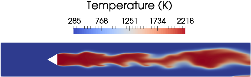
Figure 6: Instantaneous temperature contour of the reactive case on the finer LES grid.

The IPM library provides the total wall-clock execution time spent in user-designated MPI profiling sections for each MPI rank in the simulation over a single job run. Therefore, the computational time spent in, e.g., solving the chemical kinetic ODEs for each individual CFD time step cannot be obtained directly. Instead, we normalized the total wall-clock execution time by the number of CFD time steps completed in a run, and averaged the normalized wall-clock time per CFD time step over the total number of runs ($150$ for the OpenFOAM solver, and $175$ for accelerInt).

Region	Quantity	accelerInt	OpenFOAM
ODE solution	Time	$1.90\pm 0.192\text{\,}\mathrm{h}\text{/}$	$58.95\pm 8.05\text{\,}\mathrm{h}\text{/}$
	Speedup	$31.06\pm 5.27\text{\,}\times$	–
	% of total	$18.79\pm 3.32\text{\,}\mathrm{\char 37\relax}\text{/}$	$20.86\pm 2.93\text{\,}\mathrm{\char 37\relax}\text{/}$
Load balancing	Time	$7.11\pm 0.77\text{\,}\mathrm{h}\text{/}$	$254.34\pm 28.60\text{\,}\mathrm{h}\text{/}$
	Speedup	$35.82\pm 5.59\text{\,}\times$	–
	% of total	$81.06\pm 12.89\text{\,}\mathrm{\char 37\relax}\text{/}$	$78.06\pm 11.64\text{\,}\mathrm{\char 37\relax}\text{/}$
Total	Time	$9.10\pm 0.94\text{\,}\mathrm{h}\text{/}$	$313.76\pm 35.28\text{\,}\mathrm{h}\text{/}$
	Speedup	$34.48\pm 5.25\text{\,}\times$	–
	% of total

Table 7: The mean wall-clock execution time per CFD time step, speedup, and percent of total runtime spent in ODE integration and load balancing for both the accelerInt and OpenFOAM ROS4 ODE integration solvers averaged over ten runs. The times are reported in CPU hours per step, and were run on $96$ Intel E5-2690 V3 CPU cores with AVX2 vector instructions.

Table 7 presents the average wall-clock execution time per CFD time step for the accelerInt and OpenFOAM solvers. The accelerInt ROS4 solver performs, on average, $32.65$$\times$ faster (with a variation of $\pm 1.87$$\times$ depending on the run) in solving the chemical kinetic ODEs than the corresponding OpenFOAM approach. In addition, OpenFOAM poorly balances the load of the chemistry integration, with both the accelerInt and OpenFOAM chemistry solvers spending upwards of of the total computational time waiting on the solution of the chemical kinetic ODEs from other MPI ranks. OpenFOAM uses a simple static decomposition of the domain to distribute the computational cells to the various MPI ranks; hence, if a majority of the cells on an MPI rank are considered “non-reactive” (i.e., the temperature of the cell is less than the $550\text{\,}\mathrm{K}\text{/}$ threshold) the CPU core will sit idle during chemistry integration. A stiffness-based chemical kinetic load balancing scheme (e.g., as implemented by Kodavasal et al. [102]) could further improve the computational efficiency of reactive-flow simulations in OpenFOAM, and merits future investigation. Finally, Table 7 shows that the bluff-body simulation in OpenFOAM using the accelerInt solver spends $35.82\pm 5.59$$\times$ less time waiting due to poor chemical kinetic load balancing, while the overall simulation is $34.48\pm 5.25$$\times$ faster.

5 Lessons learned

Our strategy for vectorizing chemistry integration focused on building a solver based on extended versions of existing models in OpenFOAM. This consisted of

• existing turbulence-combustion interaction models (e.g., EDC, partially stirred reactor [PaSR]) to enable profiling via IPM [88];

• a batched chemistry model, based on the StandardChemistryModel class in OpenFOAM that additionally enables optional IPM profiling, that (1) scans the list of cells to determine the list of interacting cells based on the temperature cut-off, (2) converts the state variables to the form expected by pyJac, (3) passes the complete list of reacting cells to the accelerInt solver(s), and (4) finally converts state variables for the integration back to the native OpenFOAM format and stores them in the appropriate buffers;

• three solvers (each with optional IPM profiling):

  • testODE, used to verify the accuracy of the accelerInt solvers when converting to and from the OpenFOAM state variables (as compared to Cantera),

  • chemFoam, used to verify the accelerInt solver(s) coupling to OpenFOAM (i.e., integrating the system of equations), and

  • reactingFoam, used to enforce the explicit mass conservation in pyJac’s state variables, and enable the coupling to accelerInt for production simulations.

This strategy allowed us to vectorize chemistry integration while modifying little of OpenFOAM itself. Instead, almost all the logic for enabling alternate models and solvers was contained in the reactingFoamIPM module. Simultaneously, because we built the reactingFoamIPM module against existing OpenFOAM classes, we had to implement few new features there, instead using calls to the parent class wherever possible. For example, a call to the IPM-profiling-enabled PaSR class’s correction method just required placing MPI_Pcontrol calls around a call to the base PaSR class’s correction method. Thus, we did not need to vectorize OpenFOAM itself—the OpenCL code was entirely contained within the accelerInt and pyJac libraries.

We pursued an OpenCL-based strategy here to vectorize code, with the intent of supporting portability to different platforms. However, in practice, we found that this led to frequent problems involving segmentation faults during compiling, program crashes, incorrect compiled code, and more, in addition to the associated increase in complexity of the source code. Ultimately, this limited the utility of our approach. Moving forward, we recommend examining a pure OpenMP-based implementation to enable broad adoption; OpenMP version 5.0 [47, 103] might also support offloading calculations to GPUs.

6 Conclusions

This work adapted several previously developed linearly implicit and explicit OpenCL-vectorized ODE integration methods [33] into the accelerInt library [104]. We verified the accuracy of these solvers for the solution of the chemical kinetic ODEs (using source-rate and analytical Jacobian evaluation codes from the pyJac code-generation platform [35]) for a variety of cases in this effort. We developed OpenFOAM-based models of the Sandia Flame D [59, 60, 61] stabilized jet flame and Volvo bluff-body stabilized premixed flame [105]. Furthermore, we used a vectorized solver to accelerate chemical-kinetic integration of these reactive simulations, resulting in large performance improvements.

The major contributions of this work are

• Incorporating vectorized chemical kinetic ODE integration methods (provided by the accelerInt and pyJac libraries) into a publicly available OpenFOAM solver [106];

• Achieving significant speedups ($3335$$\times$) via the vectorized solvers over built-in OpenFOAM integration methods on the same hardware (an Intel Xeon CPU with AVX2 vector instructions); and

• Profiling the solution of realistic reactive-flow simulations in OpenFOAM, demonstrating the need for chemical kinetic load-balancing.

Future extensions to this work should focus on a few key aspects. First, this study has demonstrated that one of the largest bottlenecks of realistic reactive-flow simulations in OpenFOAM is the poor chemical kinetic load balancing based on static decomposition. Over of the overall computational time is wasted using either the accelerInt or native OpenFOAM solvers due to this issue. A number of chemical kinetic load balancing algorithms exist [107, 108], but the stiffness-based load-balancing technique of Kodavasal et al. [102] seems particularly promising.

More generally, this work has shown that vectorized, linearly implicit ODE integration (paired with analytical Jacobian evaluation) can greatly accelerate reactive-flow simulations. Developing vectorized sparse linear algebra/matrix factorization codes would be an excellent—while challenging—extension of this work, further speeding up the integration of larger detailed chemical models. More advanced integration algorithms should also be investigated; W-methods [49] are particularly promising for their ability to re-use previously evaluated Jacobians and LU-factorizations without needing Newton iteration.

We also found challenges in the OpenCL-based programming approach, which we originally pursued for portability. Moving forward, we recommend using pure OpenMP for vectorization, which should avoid substantially increasing source complexity and also may enable offloading of calculations to GPUs.

Appendix: Availability of material

The vectorized ODE integration methods used in this work are available in version 2.0-beta of the accelerInt library [104], while pyJac-v2.0 [109] provides the chemical kinetic source terms and Jacobian evaluation. The OpenFOAM case modeling the Volvo bluff-body flame is available for download via GitHub [105], and the coupled OpenFOAM/accelerInt solver (with IPM-based profiling) is also made available for public use [106]. Finally, the data, figures, and plotting scripts used to generate this paper are similarly available for public use [110].

References

- Imtenan et al. [2014] S. Imtenan, M. Varman, H. Masjuki, M. Kalam, H. Sajjad, M. Arbab, I. R. Fattah, Impact of low temperature combustion attaining strategies on diesel engine emissions for diesel and biodiesels: A review, Energy Convers. Manag. 80 (2014) 329–356. doi:10.1016/j.enconman.2014.01.020.
- Westbrook et al. [2005] C. K. Westbrook, Y. Mizobuchi, T. J. Poinsot, P. J. Smith, J. Warnatz, Computational combustion, Proc. Combust. Inst. 30 (2005) 125–157. doi:10.1016/j.proci.2004.08.275.
- Moiz et al. [2016] A. A. Moiz, M. M. Ameen, S.-Y. Lee, S. Som, Study of soot production for double injections of n-dodecane in CI engine-like conditions, Combust. Flame 173 (2016) 123–131. doi:10.1016/j.combustflame.2016.08.005.
- Lu and Law [2009] T. Lu, C. K. Law, Toward accommodating realistic fuel chemistry in large-scale computations, Prog. Energy Comb. Sci. 35 (2009) 192–215. doi:10.1016/j.pecs.2008.10.002.
- Turányi and Tomlin [2014] T. Turányi, A. S. Tomlin, Analysis of Kinetic Reaction Mechanisms, Springer-Verlag, Berlin Heidelberg, 2014. doi:10.1007/978-3-662-44562-4.
- Lu and Law [2006] T. Lu, C. K. Law, Linear time reduction of large kinetic mechanisms with directed relation graph: n-heptane and iso-octane, Combust. Flame 144 (2006) 24–36. doi:10.1016/j.combustflame.2005.02.015.
- Pepiot-Desjardins and Pitsch [2008] P. Pepiot-Desjardins, H. Pitsch, An efficient error-propagation-based reduction method for large chemical kinetic mechanisms, Combust. Flame 154 (2008) 67–81. doi:10.1016/j.combustflame.2007.10.020.
- Hiremath et al. [2010] V. Hiremath, Z. Ren, S. B. Pope, A greedy algorithm for species selection in dimension reduction of combustion chemistry, Combust. Theor. Model. 14 (2010) 619–652. doi:10.1080/13647830.2010.499964.
- Niemeyer et al. [2010] K. E. Niemeyer, C. J. Sung, M. P. Raju, Skeletal mechanism generation for surrogate fuels using directed relation graph with error propagation and sensitivity analysis, Combust. Flame 157 (2010) 1760–1770. doi:10.1016/j.combustflame.2009.12.022.
- Lu and Law [2007] T. Lu, C. K. Law, Diffusion coefficient reduction through species bundling, Combust. Flame 148 (2007) 117–126. doi:10.1016/j.combustflame.2006.10.004.
- Ahmed et al. [2007] S. S. Ahmed, F. Mauß, G. Moréac, T. Zeuch, A comprehensive and compact n-heptane oxidation model derived using chemical lumping, Phys. Chem. Chem. Phys. 9 (2007) 1107–1126. doi:10.1039/b614712g.
- Pepiot-Desjardins and Pitsch [2008] P. Pepiot-Desjardins, H. Pitsch, An automatic chemical lumping method for the reduction of large chemical kinetic mechanisms, Combust. Theor. Model. 12 (2008) 1089–1108. doi:10.1080/13647830802245177.
- Maas and Pope [1992] U. Maas, S. B. Pope, Simplifying chemical kinetics: intrinsic low-dimensional manifolds in composition space, Combust. Flame 88 (1992) 239–264. doi:10.1016/0010-2180(92)90034-M.
- Lam and Goussis [1994] S.-H. Lam, D. A. Goussis, The CSP method for simplying kinetics, Int. J. Chem. Kinet. 26 (1994) 461–486. doi:10.1002/kin.550260408.
- Lu et al. [2001] T. Lu, Y. Ju, C. K. Law, Complex CSP for chemistry reduction and analysis, Combust. Flame 126 (2001) 1445–1455. doi:10.1016/S0010-2180(01)00252-8.
- Gou et al. [2010] X. Gou, W. Sun, Z. Chen, Y. Ju, A dynamic multi-timescale method for combustion modeling with detailed and reduced chemical kinetic mechanisms, Combust. Flame 157 (2010) 1111–1121. doi:10.1016/j.combustflame.2010.02.020.
- Pope [1997] S. B. Pope, Computationally efficient implementation of combustion chemistry using in situ adaptive tabulation, Combust. Theor. Model. 1 (1997) 41–63. doi:10.1080/713665229.
- Ren et al. [2014] Z. Ren, Y. Liu, T. Lu, L. Lu, O. O. Oluwole, G. M. Goldin, The use of dynamic adaptive chemistry and tabulation in reactive flow simulations, Combust. Flame 161 (2014) 127–137. doi:10.1016/j.combustflame.2013.08.018.
- Li et al. [2018] Z. Li, M. T. Lewandowski, F. Contino, A. Parente, Assessment of on-the-fly chemistry reduction and tabulation approaches for the simulation of moderate or intense low-oxygen dilution combustion, Energy Fuels 32 (2018) 10121–10131. doi:10.1021/acs.energyfuels.8b01001.
- Lu and Law [2008] T. Lu, C. K. Law, Strategies for mechanism reduction for large hydrocarbons: n-heptane, Combust. Flame 154 (2008) 153–163. doi:10.1016/j.combustflame.2007.11.013.
- Niemeyer and Sung [2014] K. E. Niemeyer, C. J. Sung, Mechanism reduction for multicomponent surrogates: A case study using toluene reference fuels, Combust. Flame 161 (2014) 2752–2764. doi:10.1016/j.combustflame.2014.05.001.
- Niemeyer and Sung [2015] K. E. Niemeyer, C. J. Sung, Reduced chemistry for a gasoline surrogate valid at engine-relevant conditions, Energy Fuels 29 (2015) 1172–1185. doi:10.1021/ef5022126.
- Liang et al. [2009] L. Liang, J. Stevens, J. T. Farrell, A dynamic adaptive chemistry scheme for reactive flow computations, Proc. Combust. Inst. 32 (2009) 527–534. doi:10.1016/j.proci.2008.05.073.
- Yang et al. [2013] H. Yang, Z. Ren, T. Lu, G. M. Goldin, Dynamic adaptive chemistry for turbulent flame simulations, Combust. Theor. Model. 17 (2013) 167–183. doi:10.1080/13647830.2012.733825.
- Curtis et al. [2015] N. J. Curtis, K. E. Niemeyer, C. J. Sung, An automated target species selection method for dynamic adaptive chemistry simulations, Combust. Flame 162 (2015) 1358–1374. doi:10.1016/j.combustflame.2014.11.004.
- Mott et al. [2000] D. R. Mott, E. S. Oran, B. van Leer, A quasi-steady-state solver for the stiff ordinary differential equations of reaction kinetics, Journal of Computational Physics 164 (2000) 407–428. doi:10.1006/jcph.2000.6605.
- Hansen and Sutherland [2017] M. A. Hansen, J. C. Sutherland, Dual timestepping methods for detailed combustion chemistry, Combust. Theor. Model. 21 (2017) 329–345. doi:10.1080/13647830.2016.1235728.
- Shi et al. [2012] Y. Shi, W. H. Green, H.-W. Wong, O. O. Oluwole, Accelerating multi-dimensional combustion simulations using GPU and hybrid explicit/implicit ODE integration, Combust. Flame 159 (2012) 2388–2397. doi:10.1016/j.combustflame.2012.02.016.
- Stone and Bisetti [2014] C. P. Stone, F. Bisetti, Comparison of ODE solvers for chemical kinetics and reactive CFD applications, in: AIAA 52nd Aerospace Sciences Meeting (National Harbor, MD), 2014. doi:10.2514/6.2014-0822, AIAA Paper No. 2014-0822.
- Niemeyer and Sung [2014] K. E. Niemeyer, C. J. Sung, Accelerating moderately stiff chemical kinetics in reactive-flow simulations using GPUs, J. Comput. Phys. 256 (2014) 854–871. doi:10.1016/j.jcp.2013.09.025.
- Imren and Haworth [2016] A. Imren, D. Haworth, On the merits of extrapolation-based stiff ODE solvers for combustion CFD, Combust. Flame 174 (2016) 1–15. doi:10.1016/j.combustflame.2016.09.018.
- Curtis et al. [2017] N. J. Curtis, K. E. Niemeyer, C. J. Sung, An investigation of GPU-based stiff chemical kinetics integration methods, Combust. Flame 179 (2017) 312–324. doi:10.1016/j.combustflame.2017.02.005.
- Stone et al. [2018] C. P. Stone, A. T. Alferman, K. E. Niemeyer, Accelerating finite-rate chemical kinetics with coprocessors: comparing vectorization methods on GPUs, MICs, and CPUs, Comput. Phys. Comm. 226 (2018) 18–29. doi:10.1016/j.cpc.2018.01.015.
- Niemeyer et al. [2017] K. E. Niemeyer, N. J. Curtis, C. J. Sung, pyJac: analytical Jacobian generator for chemical kinetics, Comput. Phys. Comm. 215 (2017) 188–203. doi:10.1016/j.cpc.2017.02.004.
- Curtis et al. [2018] N. J. Curtis, K. E. Niemeyer, C. J. Sung, Using SIMD and SIMT vectorization to evaluate sparse chemical kinetic Jacobian matrices and thermochemical source terms, Combustion and Flame 198 (2018) 186–204. doi:10.1016/j.combustflame.2018.09.008.
- Hansen and Sutherland [2018] M. A. Hansen, J. C. Sutherland, On the consistency of state vectors and Jacobian matrices, Combust. Flame 193 (2018) 257–271. doi:j.combustflame.2018.03.017.
- Spafford et al. [2010] K. Spafford, J. Meredith, J. Vetter, J. Chen, R. Grout, R. Sankaran, Accelerating S3D: A GPGPU case study, in: Euro-Par 2009 Parallel Process. Workshops, LNCS 6043, Springer-Verlag, Berlin, Heidelberg, 2010, pp. 122–131. doi:10.1007/978-3-642-14122-5_16.
- Shi et al. [2011] Y. Shi, W. H. Green, H.-W. Wong, O. O. Oluwole, Redesigning combustion modeling algorithms for the graphics processing unit (GPU): Chemical kinetic rate evaluation and ordinary differential equation integration, Combust. Flame 158 (2011) 836–847. doi:10.1016/j.combustflame.2011.01.024.
- Niemeyer et al. [2011] K. E. Niemeyer, C. J. Sung, C. G. Fotache, J. C. Lee, Turbulence-chemistry closure method using graphics processing units: a preliminary test, in: Fall 2011 Technical Meeting of the Eastern States Section of the Combust. Institute, 2011. doi:10.6084/m9.figshare.3384964.
- Stone and Davis [2013] C. P. Stone, R. L. Davis, Techniques for solving stiff chemical kinetics on graphical processing units, J. Propul. Power 29 (2013) 764–773. doi:10.2514/1.B34874.
- Sewerin and Rigopoulos [2015] F. Sewerin, S. Rigopoulos, A methodology for the integration of stiff chemical kinetics on GPUs, Combust. Flame 162 (2015) 1375–1394. doi:10.1016/j.combustflame.2014.11.003.
- Curtis et al. [2017] N. J. Curtis, K. E. Niemeyer, C. J. Sung, An investigation of GPU-based stiff chemical kinetics integration methods, Combustion and Flame 179 (2017) 312–324. doi:10.1016/j.combustflame.2017.02.005.
- Kroshko and Spiteri [2013] A. Kroshko, R. J. Spiteri, Efficient SIMD solution of multiple systems of stiff IVPs, J. Comput. Sci 4 (2013) 377–385. doi:10.1016/j.jocs.2012.08.017.
- Linford and Sandu [2009] J. C. Linford, A. Sandu, Chemical kinetics on multi-core SIMD architectures, in: Proc. 9th Int. Conf. Comput. Sci., 2009.
- Linford et al. [2011] J. C. Linford, J. Michalakes, M. Vachharajani, A. Sandu, Automatic generation of multicore chemical kernels, IEEE Trans. Parallel Distrib. Syst. 22 (2011) 119–131. doi:10.1109/TPDS.2010.106.
- Che et al. [2018] Y. Che, M. Yang, C. Xu, Y. Lu, Petascale scramjet combustion simulation on the Tianhe-2 heterogeneous supercomputer, Parallel Comput. 77 (2018) 101–117. doi:10.1016/j.parco.2018.06.004.
- Dagum and Menon [1998] L. Dagum, R. Menon, OpenMP: an industry standard API for shared-memory programming, Comput. Sci. & Engineering, IEEE 5 (1998) 46–55. doi:10.1109/99.660313.
- Stone et al. [2010] J. E. Stone, D. Gohara, G. Shi, OpenCL: A parallel programming standard for heterogeneous computing systems, IEEE Des. Test 12 (2010) 66–73. doi:10.1109/MCSE.2010.69.
- Hairer and Wanner [1996] E. Hairer, G. Wanner, Solving Ordinary Differential Equations II: Stiff and Differential-Algebraic Problems, 2 ed., Springer-Verlag, Berlin, 1996. doi:10.1007/978-3-642-05221-7.
- Weller et al. [1998] H. G. Weller, G. Tabor, H. Jasak, C. Fureby, A tensorial approach to computational continuum mechanics using object-oriented techniques, Comput. Phys. 12 (1998) 620–631. doi:10.1063/1.168744.
- Kee et al. [1986] R. J. Kee, G. Dixon-Lewis, J. Warnatz, M. E. Coltrin, J. A. Miller, A Fortran computer code package for the evaluation of gas-phase multicomponent transport properties, Technical Report, Sandia National Laboratories Report SAND86-8246, 1986.
- Baum et al. [1995] M. Baum, T. Poinsot, D. Thévenin, Accurate boundary conditions for multicomponent reactive flows, J. Comput. Phys. 116 (1995) 247 – 261. doi:10.1006/jcph.1995.1024.
- Okong’o and Bellan [2002] N. Okong’o, J. Bellan, Consistent boundary conditions for multicomponent real gas mixtures based on characteristic waves, J. Comput. Phys. 176 (2002) 330 – 344. doi:10.1006/jcph.2002.6990.
- Cocks et al. [2015] P. A. Cocks, M. C. Soteriou, V. Sankaran, Impact of numerics on the predictive capabilities of reacting flow LES, Combust. Flame 162 (2015) 3394–3411. doi:10.1016/j.combustflame.2015.04.016.
- Sjunnesson et al. [1991a] A. Sjunnesson, C. Nelsson, E. Max, LDA measurements of velocities and turbulence in a bluff body stabilized flame, in: Fourth International Conference on Laser Anemometry – Advances and Application, volume 3, Cleveland, OH, 1991a, pp. 83–90.
- Sjunnesson et al. [1991b] A. Sjunnesson, S. Olovsson, B. Sjoblom, Validation rig - a tool for flame studies, in: International Symposium on Air Breathing Engines, 10th, Nottingham, England, 1991b, pp. 385–393.
- Sjunnesson et al. [1992] A. Sjunnesson, P. Henrikson, C. Lofstrom, CARS measurements and visualization of reacting flows in a bluff body stabilized flame, in: 28th Joint Propulsion Conference and Exhibit, AIAA, 1992. doi:10.2514/6.1992-3650, AIAA Paper No. 92-3650.
- Rochette et al. [2018] B. Rochette, F. Collin-Bastiani, L. Gicquel, O. Vermorel, D. Veynante, T. Poinsot, Influence of chemical schemes, numerical method and dynamic turbulent combustion modeling on LES of premixed turbulent flames, Combust. Flame 191 (2018) 417–430. doi:10.1016/j.combustflame.2018.01.016.
- Barlow and Frank [1998] R. Barlow, J. Frank, Effects of turbulence on species mass fractions in methane/air jet flames, Twenty-Seventh International Symposium on Combustion 27 (1998) 1087–1095. doi:10.1016/S0082-0784(98)80510-9.
- Barlow et al. [2005] R. Barlow, J. Frank, A. Karpetis, J.-Y. Chen, Piloted methane/air jet flames: Transport effects and aspects of scalar structure, Combust. Flame 143 (2005) 433–449. doi:https://doi.org/10.1016/j.combustflame.2005.08.017.
- Schneider et al. [2003] C. Schneider, A. Dreizler, J. Janicka, E. Hassel, Flow field measurements of stable and locally extinguishing hydrocarbon-fuelled jet flames, Combust. Flame 135 (2003) 185–190. doi:doi.org/10.1016/S0010-2180(03)00150-0.
- Bauer et al. [2014] M. Bauer, S. Treichler, A. Aiken, Singe: Leveraging warp specialization for high performance on GPUs, SIGPLAN Not. 49 (2014) 119–130. doi:10.1145/2692916.2555258.
- Intel® Corporation [2018] Intel® Corporation, OpenCL™ drivers and runtimes for Intel® architecture, https://software.intel.com/en-us/articles/opencl-drivers#latest_CPU_runtime, 2018.
- Sandu et al. [1997] A. Sandu, J. Verwer, J. Blom, E. Spee, G. Carmichael, F. Potra, Benchmarking stiff ODE solvers for atmospheric chemistry problems II: Rosenbrock solvers, Atmospheric Environ. 31 (1997) 3459–3472. doi:10.1016/S1352-2310(97)83212-8.
- Zhang and Sandu [2014] H. Zhang, A. Sandu, FATODE: A library for forward, adjoint, and tangent linear integration of odes, SIAM J. Sci. Comput. 36 (2014) C504–C523. doi:10.1137/130912335.
- Hairer et al. [1993] E. Hairer, S. P. Nørsett, G. Wanner, Solving Ordinary Differential Equations I: Nonstiff Problems, Springer Berlin Heidelberg, Berlin, Heidelberg, 1993. doi:10.1007/978-3-540-78862-1.
- Kaps et al. [1985] P. Kaps, S. W. H. Poon, T. D. Bui, Rosenbrock methods for stiff ODEs: A comparison of Richardson extrapolation and embedding technique, Comput. 34 (1985) 17–40. doi:10.1007/BF02242171.
- Shampine [1982] L. F. Shampine, Implementation of Rosenbrock methods, ACM Trans. Math. Softw. 8 (1982) 93–113. doi:10.1145/355993.355994.
- Lysenko et al. [2014] D. A. Lysenko, I. S. Ertesvåg, K. E. Rian, Numerical simulation of non-premixed turbulent combustion using the eddy dissipation concept and comparing with the steady laminar flamelet model, Flow, Turbul. Combust. 93 (2014) 577–605. doi:10.1007/s10494-014-9551-7.
- Fureby [2009] C. Fureby, Philos. Trans. Royal Soc. A: Math., Phys. Eng. Sci. 367 (2009) 2957–2969. doi:10.1098/rsta.2008.0271.
- The OpenFOAM Foundation [2018] The OpenFOAM Foundation, OpenFOAM v6 user guide, 2018. URL: https://cfd.direct/openfoam/user-guide-v6/, [Online; accessed 12/02/18].
- Message Passing Interface Forum [2012] Message Passing Interface Forum, MPI: A message-passing interface standard, version 3.0, https://www.mpi-forum.org/docs/mpi-3.0/mpi30-report.pdf, 2012.
- Weller et al. [1998] H. Weller, G. Tabor, A. Gosman, C. Fureby, Application of a flame-wrinkling LES combustion model to a turbulent mixing layer, volume 27, 1998, pp. 899–907. doi:10.1016/S0082-0784(98)80487-6.
- Magnussen [2005] B. F. Magnussen, The eddy dissipation concept–a bridge between science and technology, in: ECCOMAS thematic conference on computational combustion, 2005, pp. 21–24.
- Bösenhofer et al. [2018] M. Bösenhofer, E.-M. Wartha, C. Jordan, M. Harasek, The eddy dissipation concept—analysis of different fine structure treatments for classical combustion, Energies 11 (2018) 1902. doi:10.3390/en11071902.
- Evans et al. [2015] M. J. Evans, P. R. Medwell, Z. F. Tian, Modeling lifted jet flames in a heated coflow using an optimized eddy dissipation concept model, Combust. Sci. Tech. 187 (2015) 1093–1109. doi:10.1080/00102202.2014.1002836.
- Li et al. [2017] Z. Li, A. Cuoci, A. Sadiki, A. Parente, Comprehensive numerical study of the Adelaide jet in hot-coflow burner by means of RANS and detailed chemistry, Energy 139 (2017) 555–570. doi:10.1016/j.energy.2017.07.132.
- Magnussen [1989] B. F. Magnussen, Modeling of NOx and soot formation by the eddy dissipation concept, in: International Flame Research Foundation First Topic Oriented Technical Meeting, 1989, pp. 17–19.
- Banks et al. [2016] E. Banks, A. M. Collier, A. C. Hindmarsh, R. Serban, C. S. Woodward, SUNDIALS v2.7.0, http://computation.llnl.gov/projects/sundials-suite-nonlinear-differential-algebraic-equation-solvers/download/sundials-2.7.0.tar.gz, 2016.
- Brown et al. [1989] P. N. Brown, G. D. Byrne, A. C. Hindmarsh, VODE: a variable-coefficient ODE solver, SIAM J. Sci. Stat. Comput. 10 (1989) 1038–1051. doi:10.1137/0910062.
- Hindmarsh et al. [2005] A. C. Hindmarsh, P. N. Brown, K. E. Grant, S. L. Lee, R. Serban, D. E. Shumaker, C. S. Woodward, SUNDIALS: Suite of nonlinear and differential/algebraic equation solvers, ACM Trans. Math. Softw. 31 (2005) 363–396. doi:10.1145/1089014.1089020.
- Goodwin et al. [2018] D. G. Goodwin, H. K. Moffat, R. L. Speth, Cantera: An object-oriented software toolkit for chemical kinetics, thermodynamics, and transport processes, http://www.cantera.org, 2018. doi:10.5281/zenodo.1174508, version 2.4.0.
- Curtis and Niemeyer [2016] N. J. Curtis, K. E. Niemeyer, ch4_pasr_data.bin, Figshare, 2016. doi:10.6084/m9.figshare.4007418.v2.
- Smith et al. [1999] G. P. Smith, D. M. Golden, M. Frenklach, N. W. Moriarty, B. Eiteneer, M. Goldenberg, C. T. Bowman, R. K. Hanson, S. Song, W. C. Gardiner, V. V. Lissianski, Z. Qin, GRI-Mech 3.0, http://www.me.berkeley.edu/gri_mech/, 1999.
- The OpenFOAM Foundation [2017] The OpenFOAM Foundation, OpenFOAM v5.0, 2017. URL: https://openfoam.org/download/5-0-source/, [Online; accessed 12/02/18].
- Gabriel et al. [2004] E. Gabriel, G. E. Fagg, G. Bosilca, T. Angskun, J. J. Dongarra, J. M. Squyres, V. Sahay, P. Kambadur, B. Barrett, A. Lumsdaine, R. H. Castain, D. J. Daniel, R. L. Graham, T. S. Woodall, Open MPI: Goals, concept, and design of a next generation MPI implementation, in: Recent Advances in Parallel Virtual Machine and Message Passing Interface, Springer Berlin Heidelberg, 2004, pp. 97–104. doi:10.1007/978-3-540-30218-6_19.
- Stallman and GCC Developer Community [2009] R. M. Stallman, GCC Developer Community, Using The GNU Compiler Collection: A GNU Manual For GCC Version 4.3.3, CreateSpace, Paramount, CA, 2009.
- Skinner [2005] D. Skinner, Performance monitoring of parallel scientific applications, Technical Report, 2005. doi:10.2172/881368.
- Fureby and Moller [1995] C. Fureby, S.-I. Moller, Large eddy simulation of reacting flows applied to bluff body stabilized flames, AIAA J. 33 (1995) 2339–2347. doi:10.2514/3.12989.
- Zettervall et al. [2017] N. Zettervall, K. Nordin-Bates, E. Nilsson, C. Fureby, Large eddy simulation of a premixed bluff body stabilized flame using global and skeletal reaction mechanisms, Combust. Flame 179 (2017) 1–22. doi:10.1016/j.combustflame.2016.12.007.
- Möller et al. [1996] S. Möller, E. Lundgren, C. Fureby, Large eddy simulation of unsteady combustion, 26th International Symposium on Combustion 26 (1996) 241–248. doi:10.1016/S0082-0784(96)80222-0.
- Lee and Cant [2017] C. Y. Lee, S. Cant, Large-eddy simulation of a bluff-body stabilised turbulent premixed flame using the transported flame surface density approach, Combust. Theor. Model. 21 (2017) 722–748. doi:10.1080/13647830.2017.1293849.
- Comer [2018] A. Comer, 3rd model validation for propulsion workshop overview and validation cases, https://community.apan.org/cfs-file/__key/widgetcontainerfiles/3fc3f82483d14ec485ef92e206116d49-g-_2D00_tM6tEO4PkenM5KsnY8ctg-page-0cases/MVP3_5F00_Validation_5F00_Case_5F00_20180608.pdf, 2018. Accessed: 01-08-19.
- Comer [2016] A. Comer, Model validation for propulsion workshop - experimental data archives, 2016. URL: https://community.apan.org/wg/afrlcg/mvpws/p/experimental-data, accessed: 01-08-19.
- Smagorinsky [1963] J. Smagorinsky, General circulation experiments with the primitive equations, Mon. Weather Review 91 (1963) 99–164. doi:10.1175/1520-0493(1963)091<0099:GCEWTP>2.3.CO;2.
- Issa [1986] R. I. Issa, Solution of the implicitly discretised fluid flow equations by operator-splitting, Journal of Computational Physics 62 (1986) 40–65. doi:10.1016/0021-9991(86)90099-9.
- Weller et al. [2018] H. Weller, C. Greenshields, W. Bainbridge, OpenFOAM v6, https://openfoam.org/release/6/, 2018. Note: Commit 00e347 on the OpenFOAM-6 GitHub repository.
- Mechanical and Aerospace Engineering , University of California at San Diego(2018) [Combustion Research] Mechanical and Aerospace Engineering (Combustion Research), University of California at San Diego, Chemical-kinetic mechanisms for combustion applications, http://combustion.ucsd.edu, 2018. San Diego Mechanism web page.
- Franzelli et al. [2012] B. Franzelli, E. Riber, L. Y. Gicquel, T. Poinsot, Large eddy simulation of combustion instabilities in a lean partially premixed swirled flame, Combust. Flame 159 (2012) 621–637. doi:10.1016/j.combustflame.2011.08.004.
- Jones et al. [01 ] E. Jones, T. Oliphant, P. Peterson, et al., SciPy: Open source scientific tools for Python, 2001–. URL: http://www.scipy.org/, [Online; accessed 12/02/18].
- Virtanen et al. [2020] P. Virtanen, R. Gommers, T. E. Oliphant, M. Haberland, T. Reddy, D. Cournapeau, E. Burovski, P. Peterson, W. Weckesser, J. Bright, S. J. van der Walt, M. Brett, J. Wilson, K. J. Millman, N. Mayorov, A. R. J. Nelson, E. Jones, R. Kern, E. Larson, C. J. Carey, İ. Polat, Y. Feng, E. W. Moore, J. VanderPlas, D. Laxalde, J. Perktold, R. Cimrman, I. Henriksen, E. A. Quintero, C. R. Harris, A. M. Archibald, A. H. Ribeiro, F. Pedregosa, P. van Mulbregt, SciPy 1.0 Contributors, SciPy 1.0: fundamental algorithms for scientific computing in Python, Nature Methods 17 (2020) 261–272. doi:10.1038/s41592-019-0686-2.
- Kodavasal et al. [2016] J. Kodavasal, K. Harms, P. Srivastava, S. Som, S. Quan, K. Richards, M. García, Development of a stiffness-based chemistry load balancing scheme, and optimization of input/output and communication, to enable massively parallel high-fidelity internal combustion engine simulations, J. Energy Resour. Technol. 138 (2016) 052203. doi:10.1115/1.4032623.
- OpenMP Architecture Review Board [2021] OpenMP Architecture Review Board, OpenMP Application Program Interface version 5.2, 2021. URL: https://www.openmp.org/wp-content/uploads/OpenMP-API-Specification-5-2.pdf.
- Curtis and Niemeyer [2019] N. J. Curtis, K. E. Niemeyer, accelerInt v2.0-beta, 2019. URL: https://github.com/SLACKHA/accelerInt/tree/rewrite. doi:10.5281/zenodo.5963906.
- Curtis [2019a] N. J. Curtis, bluffbody_LES—an implementation of a Volvo Flygmotor AB bluff-body reacting flow simulation for OpenFOAM with a vectorized ODE solver, https://github.com/arghdos/bluffbody_LES, 2019a. doi:10.5281/zenodo.2574941.
- Curtis [2019b] N. J. Curtis, reactingFoamIPM-beta, Zenodo [software], version 7b46091, 2019b. URL: https://github.com/arghdos/reactingFoamIPM. doi:10.5281/zenodo.5963888.
- Flowers et al. [2006] D. L. Flowers, S. M. Aceves, A. Babajimopoulos, Effect of charge non-uniformity on heat release and emissions in PCCI engine combustion, in: SAE Technical Paper Series, 2006-01-1363, SAE International, 2006. doi:10.4271/2006-01-1363.
- Shi et al. [2009] Y. Shi, S. L. Kokjohn, H.-W. Ge, R. D. Reitz, Efficient multidimensional simulation of HCCI and DI engine combustion with detailed chemistry, in: SAE Technical Paper Series, 2009-01-0701, SAE International, 2009. doi:10.4271/2009-01-0701.
- Curtis and Niemeyer [2019] N. J. Curtis, K. E. Niemeyer, pyJac v2.0, 2019. URL: https://github.com/SLACKHA/pyJac-v2. doi:10.5281/zenodo.5964176.
- Curtis et al. [2022] N. J. Curtis, K. E. Niemeyer, C. J. Sung, Data, plotting scripts, and figures for “Accelerating reactive-flow simulations using vectorized chemistry integration”, Zenodo [dataset], 2022. doi:10.5281/zenodo.5963861.