NTIRE 2022 Challenge on Efficient Super-Resolution: Methods and Results
Abstract
This paper reviews the NTIRE 2022 challenge on efficient single image super-resolution with focus on the proposed solutions and results. The task of the challenge was to super-resolve an input image with a magnification factor of 4 based on pairs of low and corresponding high resolution images. The aim was to design a network for single image super-resolution that achieved improvement of efficiency measured according to several metrics including runtime, parameters, FLOPs, activations, and memory consumption while at least maintaining the PSNR of 29.00dB on DIV2K validation set. IMDN is set as the baseline for efficiency measurement. The challenge had 3 tracks including the main track (runtime), sub-track one (model complexity), and sub-track two (overall performance). In the main track, the practical runtime performance of the submissions was evaluated. The rank of the teams were determined directly by the absolute value of the average runtime on the validation set and test set. In sub-track one, the number of parameters and FLOPs were considered. And the individual rankings of the two metrics were summed up to determine a final ranking in this track. In sub-track two, all of the five metrics mentioned in the description of the challenge including runtime, parameter count, FLOPs, activations, and memory consumption were considered. Similar to sub-track one, the rankings of five metrics were summed up to determine a final ranking. The challenge had 303 registered participants, and 43 teams made valid submissions. They gauge the state-of-the-art in efficient single image super-resolution.
1 Introduction
Single image super-resolution (SR) aims at recovering a high-resolution (LR) image from a single low-resolution (LR) image that undergoes certain degradation process. Before the deep learning era, the problem of image SR is tackled by reconstruction-based [8, 19, 61] and exampled-based methods [20, 68, 69, 62]. With the thriving of deep learning, SR is frequently tackled by solutions based on deep neural networks [15, 35, 37, 48, 84, 47].
For image SR, it is assumed that the LR image is derived after two major degradation processes including blurring and down-sampling, namely,
| (1) |
where denotes the convolution operation between the LR image and the blur kernel and is the down-sampling operation with a down-scaling factor of . Depending on the blur kernel and the down-sampling operation, image SR could be classified into several standard problems. And among them, bicubic down-sampling with different down-scaling factors (, , , , or even ) is the most frequently used degradation model. This classical standard degradation model allows direct comparison between different image SR methods, which also serves as a test bed to validate the advantage a newly proposed SR method.
With the fast development of hardware technologies, it becomes possible to train much larger and deeper neural networks for image SR, which contributes significantly to the performance boost of the proposed solutions. Almost each breakthrough in the field of image SR comes with a more complex deep neural network [15, 35, 37, 48, 88, 47]. Apart from the development of large models with high performance, a parallel direction is design efficient deep neural networks for single image SR [16, 66, 40, 32, 31, 23, 85]. In [16, 66], the proposed networks extracted features directly from the LR images instead of the bicubic interpolation of the LR image, which saved the computation by almost a factor of . This laid the foundation for later design of neural networks for image SR. Later works focused on the design of basic building blocks from different perspectives [40, 32, 31]. In [23], a new activation function, namely multi-bin trainable linear unit was proposed to increase the nonlinear modeling capacity of shallow network. In [85], an edge-oriented convolution block is proposed for real-time SR on mobile devices.
Besides the manual design of deep neural networks, there are a plethora of works that try to improve the efficiency of deep neural networks via network pruning [27, 55, 43, 44, 39], low-rank filter decomposition [87, 33, 41, 42], network quantization [25, 11], neural architecture search [50, 67, 76], and knowledge distillation [28, 70]. Among those network compression works, a couple of them have been successfully applied to image SR [42, 43, 44, 67, 76].
The efficiency of deep neural network could be measured in different metrics including runtime, number of parameters, computational complexity (FLOPs), activations, and memory consumption, which affect the deployment of deep neural network in different aspects. Among them, runtime is the most direct indicator of the efficiency of a network and thus is used as the main efficiency evaluation metric. The number of activations and parameters is related to memory consumption. And a higher memory consumption means that additional memory devices are needed to store the activations and parameters during the inference. Increased computational complexity is related to higher energy consumption, which could shorten the battery life of mobile devices. At last, the number of parameters is also related to AI chip design. More parameters mean larger chip area and increased cost of the designed AI devices.
Jointly with the 2022 New Trends in Image Restoration and Enhancement (NTIRE 2022) workshop, we organize the challenge on efficient super-resolution. The task of the challenge is to super-resolve an LR image with a magnification factor of 4 by a network that reduces one or several aspects such as runtime, parameters, FLOPs, activations and memory consumption, while at least maintaining PSNR of 29.00dB on the DIV2K validation set. The challenge aims to seek advanced and novel solutions for efficient SR, to benchmark their efficiency, and identify the general trends for the design of efficient SR networks.
2 NTIRE 2022 Efficient Super-Resolution Challenge
This challenge is one of the NTIRE 2022 associated challenges on: spectral recovery [4], spectral demosaicing [3], perceptual image quality assessment [22], inpainting [63], night photography rendering [18], efficient super-resolution [46], learning the super-resolution space [56], super-resolution and quality enhancement of compressed video [78], high dynamic range [60], stereo super-resolution [71], burst super-resolution [7].
The objectives of this challenge are: (i) to advance research on efficient SR; (ii) to compare the efficiency of different methods and (iii) to offer an opportunity for academic and industrial attendees to interact and explore collaborations. This section details the challenge itself.
2.1 DIV2K Dataset [2]
Following [2, 83, 82], the DIV2K dataset is adopted for the challenge. The dataset contains 1,000 DIVerse 2K resolution RGB images, which are divided into a training set with 800 images, a validation set with 100 images, and a testing with 100 images. The corresponding LR DIV2K in this challenge is the bicubicly downsampled counterpart with a down-scaling factor . The validation set is already released to the participants. The testing HR images are hidden from the participants during the whole challenge.
2.2 IMDN Baseline Model
The IMDN [31] serves as the baseline model in this challenge. The aim is to improve its efficiency in terms of runtime, number of parameters, FLOPs, number of activations, and GPU memory consumption while maintaining a PSNR performance of 29.00dB on the validation set. The IMDN model uses a convolution to extract features from the LR RGB images, which is followed by 8 information multi-distillation blocks. The information multi-distillation block contains 4 stages that progressive refine the feature representation in the block. In each stage, the input feature from the previous stage is split along the channel dimension, leading two separated features. Among the two features, one is bypassed to the end of the block and the other one is fed to the next stage for the calculation of high-level feature. The bypassed features from the 4 stages are concatenated along the channel dimension and combined by a convolution. The final upsampler only consists of one trainable convolutional layer to expand the feature dimension. Pixel-shuffle is used to recover the high-resolution grid of the image. This design is considered to save as many parameters as possible.
The baseline IMDN is provided by the winner of the AIM 2019 Challenge on Constrained Super-Resolution [83]. The quantitative performance and efficiency metrics of IMDN are given in Tab. 1 and summarized as follows. (1) The number of parameters is 0.894M. (2) The average PSNRs on validation and testing sets of DIV2K are 29.13dB and 28.78dB, respectively. (3) The runtime averaged on the validation and test set with PyTorch 1.11.0, CUDA Toolkit 10.2, cuDNN 7.6.2 and a single Titan Xp GPU is 50.86 ms. (4) The number of FLOPs for an input of size is 58.53G. (5) The number of activations (i.e. the number of elements in all convolutional layer outputs) for an input of size is 154.14M. (5) The maximum GPU memory consumption during the inference on the DIV2K validation set is 471.76M. (6) The number of convolutional layers is 43.
2.3 Tracks and Competition
The aim of this challenge is to devise a network that reduces one or several aspects such as runtime, parameters, FLOPs, activations and memory consumption while at least maintaining the PSNR of 29.00dB on the validation set. The challenge is divided into three tracks according to the 5 evaluation metrics.
Main Track: Runtime Track. In this track, the practical runtime performance of the submissions is evaluated. The rankings of the teams are determined directly by the absolute value of the average runtime on the validation set and test set.
Sub-Track 1: Model Complexity Track. In this track, the number of parameters and FLOPs are considered. And the rankings of the two metrics are summed up to determine a final ranking in this track.
Sub-Track 2: Overall Performance Track. In this track, all of the five metrics mentioned in the description of the challenge including runtime, parameters, FLOPs, activations, and GPU memory are considered. Similar to Sub-Track 1, the rankings of five metrics are summed up to determine a final ranking in this track.
Ranking statistic When determine the ranking in the case of multiple metrics, the individual rankings of different metrics are summed up, which constitutes a ranking statistic of the metrics. This idea is similar to that behind Spearman’s correlation. That is, instead of using the absolute values, a ranking statistic could remove the influence of unit and at the same time be good enough to distinguish different entries.
Challenge phases (1) Development and validation phase: The participants had access to the 800 pairs of LR/HR training image pairs and 100 pairs of LR/HR validation images of the DIV2K dataset. The IMDN model, pretrained parameters, and validation demo script are given on GitHub (https://github.com/ofsoundof/IMDN), allowing the participants to benchmark the runtime of their models on their system. The participants could upload the HR validation results on the evaluation server to calculate the PSNR of the super-resolved image produced by their models to get immediate feedback. The number of parameters and runtime was computed by the participant. (2) Testing phase: In the final test phase, the participants were granted access to the 100 LR testing images. The HR ground-truth images are hidden for the participants. The participants then submitted their super-resolved results to the Codalab evaluation server and e-mailed the code and factsheet to the organizers. The organizers verified and ran the provided code to obtain the final results. Finally, the participants received the final results at the end of the challenge.
| Team | Main Track | Sub- Track 1 | Sub- Track 2 | PSNR [Val.] | PSNR [Test] | Ave. Time [ms] | #Params [M] | FLOPs [G] | #Acts [M] | GPU Mem. [M] | #Conv |
| ByteESR | 1 | 22(11) | 33(2) | 29.00 | 28.72 | 27.11(1) | 0.317(11) | 19.70(11) | 80.05(6) | 377.91(4) | 39 |
| NJU_Jet | 2 | 37(18) | 44(6) | 29.00 | 28.69 | 28.07(2) | 0.341(18) | 22.28(19) | 72.09(4) | 204.60(1) | 34 |
| NEESR | 3 | 10(4) | 27(1) | 29.01 | 28.71 | 29.97(3) | 0.272(4) | 16.86(6) | 79.59(5) | 575.99(9) | 59 |
| Super | 4 | 26(12) | 55(10) | 29.00 | 28.71 | 32.09(4) | 0.326(14) | 20.06(12) | 93.82(10) | 663.07(15) | 59 |
| MegSR | 5 | 18(9) | 43(5) | 29.00 | 28.68 | 32.59(5) | 0.290(9) | 17.70(9) | 91.72(8) | 640.63(12) | 64 |
| rainbow | 6 | 16(8) | 34(3) | 29.01 | 28.74 | 34.10(6) | 0.276(6) | 17.98(10) | 92.80(9) | 309.23(3) | 59 |
| VMCL_Taobao | 7 | 29(14) | 57(11) | 29.01 | 28.68 | 34.24(7) | 0.323(13) | 20.97(16) | 98.67(11) | 633.00(10) | 40 |
| Bilibili AI | 8 | 15(7) | 41(4) | 29.00 | 28.70 | 34.67(8) | 0.283(8) | 17.61(7) | 90.50(7) | 633.74(11) | 64 |
| NKU-ESR | 9 | 12(5) | 48(7) | 29.00 | 28.66 | 34.81(9) | 0.276(7) | 16.73(5) | 111.12(13) | 662.51(14) | 65 |
| NJUST_RESTORARION | 10 | 54(27) | 89(15) | 28.99 | 28.68 | 35.76(10) | 0.421(28) | 27.67(26) | 108.66(12) | 643.95(13) | 52 |
| TOVBU | 11 | 43(21) | 96(19) | 29.00 | 28.71 | 38.32(11) | 0.376(23) | 22.38(20) | 113.55(15) | 867.17(27) | 64 |
| Alpan Team | 12 | 18(10) | 51(9) | 29.01 | 28.75 | 39.63(12) | 0.326(15) | 12.31(3) | 115.52(16) | 439.37(5) | 132 |
| Dragon | 13 | 38(19) | 70(13) | 29.01 | 28.69 | 41.80(13) | 0.358(20) | 21.11(18) | 120.15(17) | 260.00(2) | 131 |
| TieGuoDun Team | 14 | 54(27) | 104(21) | 28.95 | 28.65 | 42.35(14) | 0.433(29) | 27.10(25) | 112.03(14) | 788.13(22) | 64 |
| HiImageTeam | 15 | 7(3) | 70(13) | 29.00 | 28.72 | 47.75(15) | 0.242(3) | 14.51(4) | 151.36(23) | 861.84(25) | 100 |
| xilinxSR | 16 | 66(34) | 107(22) | 29.05 | 28.75 | 48.20(16) | 0.790(34) | 51.76(32) | 136.31(18) | 471.37(7) | 38 |
| cipher | 17 | 50(24) | 111(23) | 29.00 | 28.72 | 51.42(17) | 0.407(26) | 25.25(24) | 155.35(24) | 770.82(20) | 67 |
| NJU_MCG | 18 | 13(6) | 66(12) | 28.99 | 28.71 | 52.02(18) | 0.275(5) | 17.65(8) | 212.35(27) | 511.08(8) | 84 |
| IMGWLH | 19 | 34(17) | 91(17) | 29.01 | 28.72 | 56.34(19) | 0.362(21) | 20.10(13) | 136.35(19) | 753.02(19) | 113 |
| imglhl | 20 | 45(22) | 92(18) | 29.03 | 28.75 | 56.88(20) | 0.381(24) | 23.26(21) | 144.05(21) | 451.21(6) | 127 |
| whu_sigma | 21 | 63(32) | 132(30) | 29.02 | 28.73 | 61.04(21) | 0.705(33) | 43.88(30) | 142.91(20) | 1011.54(28) | 64 |
| Aselsan Research | 22 | 27(13) | 98(20) | 29.02 | 28.73 | 63.18(22) | 0.317(12) | 20.71(15) | 206.05(26) | 799.52(23) | 134 |
| Drinktea | 23 | 59(31) | 121(27) | 29.00 | 28.70 | 75.52(23) | 0.589(31) | 36.92(28) | 148.05(22) | 734.54(17) | 67 |
| GDUT_SR | 24 | 50(24) | 136(31) | 29.05 | 28.75 | 75.70(24) | 0.414(27) | 24.80(23) | 260.05(28) | 1457.98(34) | 195 |
| Giantpandacv | 25 | 63(32) | 150(34) | 29.07 | 28.76 | 87.87(25) | 0.683(32) | 45.07(31) | 361.23(31) | 1272.95(31) | 122 |
| neptune | 26 | 39(20) | 123(29) | 28.99 | 28.69 | 101.69(26) | 0.316(10) | 38.03(29) | 269.48(29) | 1179.05(29) | 45 |
| XPixel | 27 | 3(1) | 49(8) | 29.01 | 28.69 | 140.47(27) | 0.156(1) | 9.50(2) | 65.76(3) | 729.94(16) | 43 |
| NJUST_ESR | 28 | 3(1) | 89(15) | 28.96 | 28.68 | 164.80(28) | 0.176(2) | 8.73(1) | 160.43(25) | 1346.74(33) | 25 |
| TeamInception | 29 | 57(30) | 146(33) | 29.12 | 28.82 | 171.56(29) | 0.505(30) | 32.42(27) | 502.27(34) | 866.16(26) | 74 |
| cceNBgdd | 30 | 33(16) | 114(24) | 28.97 | 28.67 | 180.60(30) | 0.339(16) | 21.11(17) | 404.16(33) | 739.65(18) | 197 |
| ZLZ | 31 | 55(29) | 118(26) | 29.00 | 28.72 | 183.43(31) | 0.372(22) | 64.45(33) | 57.51(2) | 1244.23(30) | 16 |
| Express | 32 | 31(15) | 117(25) | 29.04 | 28.77 | 203.16(32) | 0.339(17) | 20.41(14) | 325.53(30) | 853.27(24) | 148 |
| Just Try | 33 | 70(35) | 170(35) | 29.12 | 28.81 | 247.90(33) | 0.832(35) | 135.30(35) | 392.43(32) | 2387.93(35) | 207 |
| ncepu_explorers | 34 | 47(23) | 137(32) | 29.09 | 28.79 | 317.66(34) | 0.390(25) | 23.73(22) | 994.25(35) | 771.54(21) | 374 |
| mju_mnu | 35 | 53(26) | 121(27) | 29.06 | 28.79 | 332.28(35) | 0.345(19) | 78.81(34) | 46.76(1) | 1310.72(32) | 40 |
| The following methods are not ranked since their validation/testing PSNR are not on par with the baseline. | |||||||||||
| Virtual_Reality Team | 27.35 | 27.26 | 2231.32 | 0.423 | 423.16 | 2731.08 | 3336.88* | 82 | |||
| NTU607QCO-ESR | 27.79 | 27.61 | 38.85 | 0.433 | 27.06 | 108.89 | 776.38 | 60 | |||
| Strong Tiger | 29.00 | 28.61 | 34.92 | 0.560 | 36.64 | 78.91 | 641.13 | 23 | |||
| VAP | 29.01 | 28.47 | 23.96 | 0.175 | 10.83 | 70.93 | 507.64 | 63 | |||
| Multicog | 28.38 | 28.16 | 207.98 | 0.312 | 37.67 | 430.23 | 1461.57 | 130 | |||
| Set5baby Team | 28.92 | 28.62 | 83.44 | 0.223 | 13.98 | 229.07 | 797.25 | 88 | |||
| NWPU_SweetDreamLab | 28.47 | 28.23 | 31.19 | 0.193 | 11.73 | 90.50 | 633.10 | 76 | |||
| SSL | 28.72 | 28.44 | 64.71 | 0.290 | 18.95 | 150.60 | 675.41 | 48 | |||
| RFDN AIM2020 Winner | 29.04 | 28.75 | 41.97 | 0.433 | 27.10 | 112.03 | 788.13 | 64 | |||
| IMDN_baseline | 29.13 | 28.78 | 50.86 | 0.894 | 58.53 | 154.14 | 471.76 | 43 | |||
-
*
This solution uses too much GPU memory. Images are cropped to with 32 overlapping pixels during inference.
Evaluation protocol The quantitative evaluation metrics include validation and testing PSNRs, runtime, number of parameters, number of FLOPs, number of activations, and maximum GPU memory consumed during inference. The PSNR was measured by first discarding the 4-pixel boundary around the images. The the average runtime during the inference on the 100 LR validation images and the 100 LR testing images is computed. The best runtime among three consecutive trails is selected as the final result. The average runtime on the validation set and testing set is used as the final runtime indicator. The maximum GPU memory consumption is recorded during the inference. The FLOPs, activations are evaluated on an input image of size . Among the above metrics, the runtime is regarded as the most important one. During the challenge, the participants are required to maintain the PSNR of 29.00dB on the validation set. For the final ranking, a tiny accuracy drop is tolerated. To be specific, submissions with PSNR higher than 28.95dB on the validation set and 28.65dB on the testing set could enter the final ranking. The constraint on the testing set avoids overfitting on the validation set. A code example for calculating these metrics is available at https://github.com/ofsoundof/NTIRE2022_ESR. The code of the submitted solutions and the pretrained weights are also available in this repository.
3 Challenge Results
Tab. 1 reports the final test results and rankings of the teams. The solutions with validation PSNR lower than 28.95dB and test PSNR lower than 28.65dB are not ranked. The results of the baseline method IMDN [31] and the overall first place winner team in AIM 2020 Efficient SR challenge [51] are also reported for comparison. The methods evaluated in Tab. 1 are briefly described in Sec. 4 and the team members are listed in Appendix A. According to Tab. 1, we can have the following observations.
Main Track: Runtime Track. First, the ByteESR team is the overall first place winner in the main track of this efficient SR challenge. The NJU_Jet team and NEESR team win the overall second place and overall third place, respectively. The average runtime of the first three solutions is below 30 ms and is very close to each other. The first 12 teams proposed a solution with average runtime lower than 40 ms. In addition, the solution proposed by the 13-th team is also faster than the AIM 2020 winnder RFDN [51].
Sub-Track 1: Model Complexity Track For this track, there are two first place winners including XPixel and NJUST_ESR. The solution proposed by XPixel team has slightly fewer parameters while the solution proposed by NJUST_ESR team has fewer computation. The HiImageTeam team achieves the third place in this track. The number of parameters of 9 solutions are lower than 0.3 M, which is a significant improvement compared with the AIM 2019 constrained SR challenge winner IMDN and the AIM 2020 efficient SR challenge winner RFDN. As for the computational complexity, the FLOPs of 11 solutions is lower than 20G and 27 solutions have fewer FLOPs than RFDN.
Sub-Track 2: Overall Performance Track The NEESR team is the first place winner in this track. ByteESR and rainbow are the second and third place winner in this track, respectively. The solutions proposed by mju_mnu, ZLZ, and NJUST_ESR team have the least number of activations. Meanwhile, the solutions proposed by NJU_Jet, Dragon, and rainbow team are among the most memory-efficient solutions.
The xilinxSR team achieved the best PSNR fidelity metric (29.05dB on the validation set and 29.75dB on test set) among the solutions that outperforms the baseline network IMDN in terms of runtime and number of parameters. When comparing this solution and the baseline solution IMDN, it is observed that IMDN has a larger PSNR improvement on the validation set than on the test set. On the other hand, it is also observed that, compared with the solutions proposed by TeamInception and Just Try, IMDN has similar PSNR on the validation set but achieves lower PSNR on the test set. Such phenomenons indicate that IMDN is more in favor of the PSNR on validation set. This is also the reason why the baseline PSNR on the validation set is set to 29.00dB rather than 29.13dB.
3.1 Architectures and main ideas
During this challenge, a couple of techniques are proposed to improve the efficiency of deep neural network for image SR while maintaining the performance as much as possible. Depending on the metrics that a team wants to optimize, different solutions are proposed. In the following, some typical ideas are listed.
-
1.
Modifying the architecture of information multi-distillation block (IMDB) and residual feature distillation block (RFDB) is the mainstream technique. The IMDB and RFDB modules come from the first place winners of the AIM 2019 constrained image SR challenge and the AIM 2020 efficient image SR challenge. Thus, some teams of this challenge start from modifying those two basic architectures. The first place winner ByteESR in the runtime main track proposed a residual local feature block (RLFB) to replace the RFDB and IMDB modules. The main difference is the removal of the concatenation operation and the associated convolutional feature distillation layers. This is optimized especially out of runtime considerations. Besides, the team also reduced the number of convolutions in the ESA module.
-
2.
Multi-stage information distillation might influence the inference speed of the super efficient models. It is observed that the first two place solutions in the runtime main track do not contain multi-stage information distillation blocks in the network. It is also reported in other work [85] that using too many skip connections and associated information distillation layers could harm the runtime performance.
-
3.
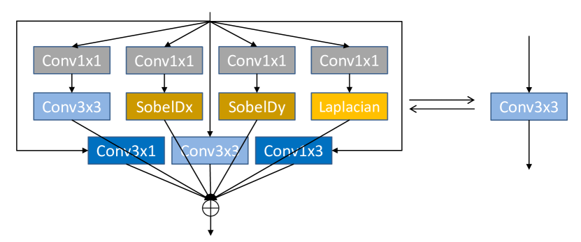
Reparameterization could bring slight performance improvement. A couple of teams tried to reparameterize a normal convolutional layer with multiple basic operations ( convolution, operation, first and second order derivative operators, skip connections) during network training. During inference, the multiple operations that reparameterize a convolution could be merged back to a single convolution. It is demonstrated that, this technique could bring slight PSNR gain. For example, NJU_Jet replaced a normal residual block with a reparameterized residual block. The NEESR team used edge-oriented convolution block to reparameterize a normal convolution.
-
4.
Filter decomposition methods could effectively reduce the model complexity. Filter decomposition method generally refers to the replacement of a normal convolution by a couple of lightweight convolutions (depthwise, , and convolutions). For example, the XPixel used the combination of depthwise convolution and convolution. The NJUST_ESR team also used the inverted residual block. And the solutions proposed by the two team won the first two places in the model complexity track.
-
5.
Network pruning began to play a role. It is observed that a couple of teams used network pruning techniques to slightly compress a baseline network. For example, the ByteESR team slightly pruned the number of channels in their network from 48 to 46 at the final training stage. The MegSR team normalized the weight parameters and applied learnable parameters to the normalized channels. They pruned the network according to the magnitude of these parameters. The xilinxSR team also tried to prune the IMDB modules.
-
6.
Activation function is an important factor. It is observed that some team used advanced activation function in their network. For example, the rainbow team used SiLU activation function for each convolution except the last convolution. A lot of teams also used GeLU activation function.
-
7.
Design of loss functions is also among the consideration. Loss function is also an important element for the success of an efficient SR network. While most of the teams used L1 or L2 loss, some teams also demonstrated using a more advanced loss function could bring marginal PSNR gain. For example, the ByteESR team used contrastive loss to improve the PSNR by 0.01dB - 0.02dB on different validation sets. The NKU-ESR team proposed edge-enhanced gradient-variance loss.
-
8.
Advanced training strategy guarantees the performance of the network. The advanced training strategy contains many aspects of the training setting. For example, most of the teams prolonged the training. Since the size of models is mostly small, training with both large patch size and batch size becomes possible. Periodic learning rate scheduler and cosine learning rate scheduler are used by some team, which could help the training to step outside of the local minima. The training of winner solutions typically contains several stages. Advanced tuning of the network architecture such as pruning and merging of reparameterized operations is used at the final fine-tuning stages.
-
9.
Various other techniques are also attempted. Some teams also proposed solutions based on neural architecture search, vision transformers, and even fast Fourier transform.
3.2 Participants
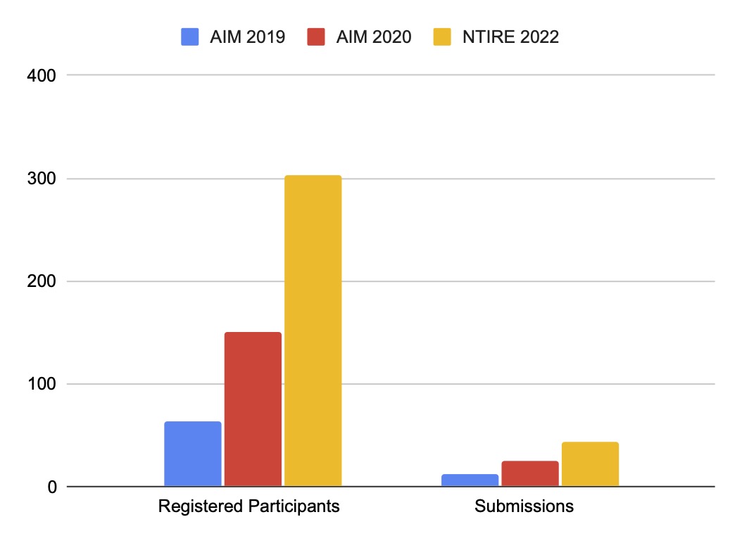
This year we see a continuous growth of the efficient SR challenge with more participants and valid submission. As shown in Fig. 1, the number of registered participants grows from 64 in AIM 2019, 150 in AIM 2020, and finally 303 in this year. Meanwhile, the number of valid submission also grows from 12 in AIM 2019, 25 in AIM 2020, and 43 this year.
3.3 Fairness
To maintain the fairness of the efficient SR challenge, a couple of rules about fair and unfair tricks are set. Most of the rules are about the dataset used to train the network. First, training with additional external dataset such as Flickr2K is allowed. Secondly, training with the additional DIV2K validation set including either of the HR or LR images is not allowed. This is because the validation set is used to examine the overall performance and generalizability of the proposed network. Thirdly, training with the DIV2K test LR images is not allowed. Fourthly, training with advanced data augmentation strategy during training is regarded as a fair trick.
3.4 Conclusions
Based on the aforementioned analysis of the efficient SR challenge results, the following conclusions can be drawn.
-
1.
The efficient image SR community is growing. This year the challenge had 303 registered participants, and received 43 valid submissions, which is a significant boost compared with the previous years.
-
2.
The family of the proposed solutions during this challenge keep to push the frontier of the research and implementation of efficient images SR.
-
3.
In conjunction with the previous series of the efficient SR challenge including AIM 2019 Constrained SR Challenge [83] and AIM 2020 Efficient SR Challenge [82], the proposed solutions make new records of network efficiency in term of metrics such as runtime and model complexity while maintain the accuracy of the network.
-
4.
There is a divergence between the actual runtime and theoretical model complexity of the proposed networks. This shows that the theoretical model complexity including FLOPs and the number of parameters do not correlate well with the actual runtime at least on GPU infrastructures.
-
5.
In the meanwhile, new developments in the efficient SR field are also observed, which include but not limited to the following aspects.
-
•
The effectiveness of multi-stage information distillation mechanism is challenged by the first two place solutions in the runtime main track.
-
•
Other techniques such as contrastive loss, network pruning, and convolution reparameterization began to play a role for efficient SR.
-
•
4 Challenge Methods and Teams
4.1 ByteESR

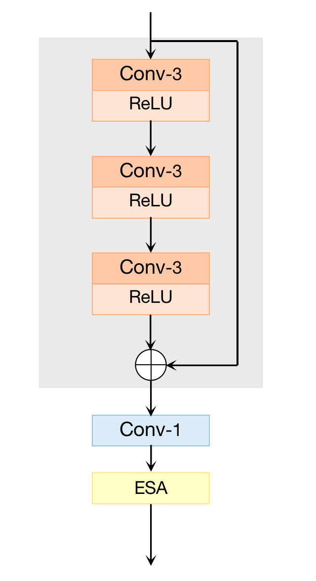
Network Architecture The ByteESR Team proposed Residual Local Feature Network (RLFN) for Efficient Super-Resolution. As shown in Fig. 3, the proposed RLFN uses one of the basic SR architecture, which is similar to IMDN [31] and other methods [48, 74]. The difference is RLFN uses four residual local feature block (RLFB) as the building blocks.
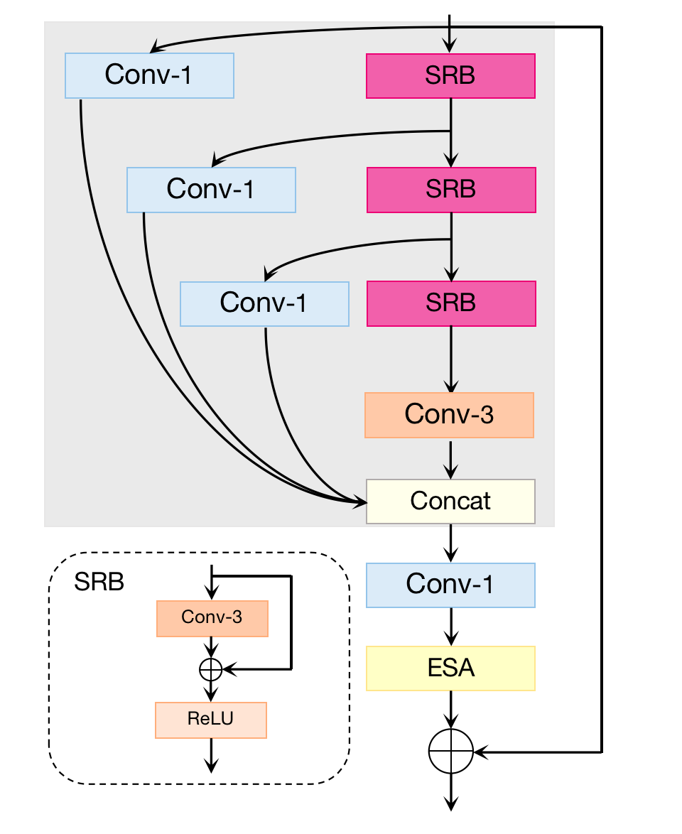
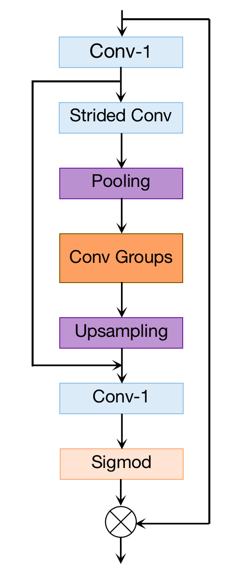
The proposed RLFN is modified from residual feature distillation block (RFDB) [51]. As shown in Fig. 2(a), RFDB uses three Conv-1 for feature distillation, and all the distilled features are concatenated together. Although aggregating multiple layers of distilled features can result in more powerful feature, concatenation accounts for most of the inference time. Based on the consideration of reducing inference time and memory, RLFB (see Fig. 2(b)) removes the concatenation layer and the related feature distillation layers and replaces them with an addition for local feature learning. Besides, in RLFB, the Conv Groups in ESA [52] (see Fig. 2(c)) is simplified to one Conv-3 to decrease the model depth and complexity.

Contrastive Loss Some recent works [53, 72] find that a randomly initialized feature extractor, without any training, can be used to improve the performance of models on several dense prediction tasks. Inspired by these works, RLFN builds a two-layer network as the feature extractor. The weights of convolution kernels are randomly initialized. The contrastive loss is defined as:
| (2) |
where defines the feature map generated by the feature extractor, is the L1 distance loss between feature maps of and and is the L1 distance loss between feature maps of and .
Implementation details. The proposed RLFN has four RLFBs, in which the number of feature channels is set to 48 while the channel number of ESA is set to 16. During training, DIV2K [2] and Flickr2K datasets are used for the whole process. The details of training steps are as follows:
-
I.
At the first stage, the model is trained from scratch. HR patches of size are randomly cropped from HR images, and the mini-batch size is set to 64. The RLFN model is trained by minimizing L1 loss function with Adam optimizer. The initial learning rate is set to and halved at every 200 epochs.The total number of epochs is 1000.
-
II.
At the second stage, the model is initialized with the pretrained weights, and trained with the same settings as in the previous step. This process repeats twice.
-
III.
At the third stage, the model is initialized with the pretrained weights from Stage 2. The same training settings as Stage 1 are kept to train the model, except that the loss function is replaced by the combination of L1 loss and contrastive loss with a regularization factor .
-
IV.
At the fourth stage, the number of Conv-1 of RLFBs in the pretrained model from 48 to 46 using Soft Filter Pruning [26]. Training settings are the same as Stage 1, except that the size of HR patches changes to . After 1000 epochs, L2 loss is used for fine-tuning with HR patches and a learning rate of .
4.2 NJU_Jet
Runtime and memory consumption are two important aspects for efficient image super-resolution (EISR) models to be deployed on resource-constrained devices. Recent advances in EISR[31, 51] exploit distillation and aggregation strategies with plenty of channel split and concatenation operations to make full use of limited hierarchical features. By contrast, sequential network operations avoid frequently accessing preceding states and extra nodes, and thus are beneficial to reducing the memory consumption and runtime overhead. Following this idea, the team designed a lightweight network backbone by mainly stacking multiple highly optimized convolution and activation layers and decreasing the usage of feature fusion. The overall network architecture is shown in Fig. 4. The feature extraction part and reconstruction part are the same as recent works [31, 51], and the high-frequency learning part is composed of the proposed enhanced residual block (ERB) and high-frequency attention block (HFAB) pairs.
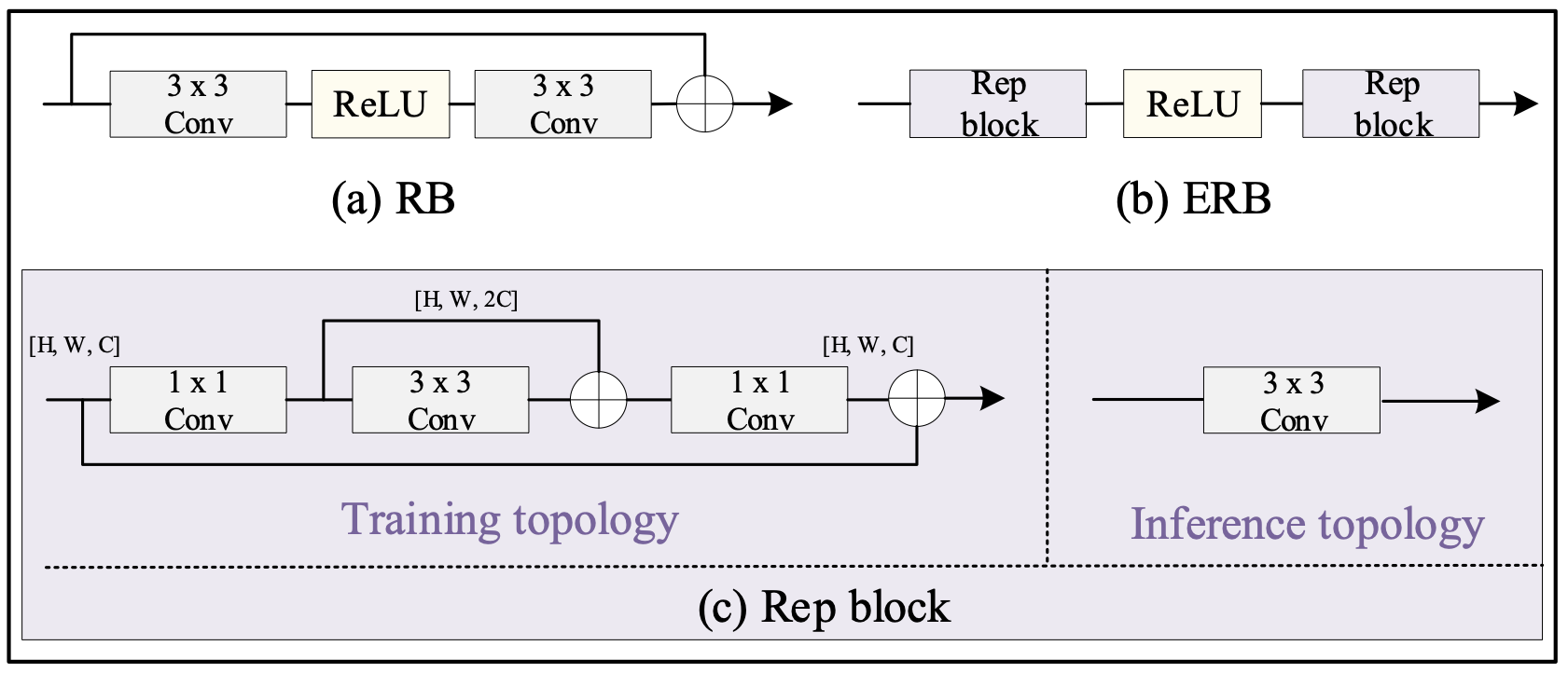
Enhanced residual block. The team first proposed enhanced residual block (ERB) to replace normal residual block (RB) in EDSR [48], for reducing the memory access cost (MAC) introduced by skip connection. As shown in Fig. 5, ERB is composed of two re-parameterization blocks (RepBlock) and one ReLU. During training, each RepBlock utilizes convolution to expand or reduce the number of feature maps and adopts convolution to extract features in higher dimensional space. Besides, two skip connections are used to ease training difficulty. During inference, all the linear transformations can be merged [14]. Thus each RepBlock can be converted into a single convolution. In general, ERB takes advantage of residual learning without additional MAC.
High-frequency attention block. Recently, attention mechanism has been extensively studied in the SR community. Based on the grain-size composition, it can be divided into channel attention [34, 31], spatial attention [75], pixel attention [90], and layer attention [59]. Previous attention-based methods lack consideration of two important aspects. First, some attention schemes, such as CCA [31] and ESA [51], have multi-branch topology, which introduces too much extra memory consumption. Second, some nodes in the attention branch are not computationally optimal, such as convolution used in ESA [52], which is much less efficient than convolution.
Considering both aspects, a sequential attention branch is designed to rescale each position based on its nearby pixels. The attention branch is inspired by edge detection, where the linear combination of nearby pixels can be used to detect edges. Furthermore, the team found out that the attention branch focused on high-frequency areas and named the proposed block as high-frequency attention block (HFAB) shown in Fig. 4. HFAB rescales every position according to the non-linear combination of its window. In HFAB, convolution rather than convolution is used to reduce and expand feature dimension for larger receptive field and efficiency. Batch normalization (BN) is adopted in the attention branch to introduce global statistics and to keep features within the unsaturated area of sigmoid function. During inference, BN can be merged into convolution without additional computational cost.
Implementation details. DIV2K and Flickr2K are used as the training dataset. Five ERB-HFAB pairs are stacked sequentially. The number of feature maps of ERB and HFAB is set to 50 and 16, respectively. In each training batch, 64 HR RGB patches are cropped with size and augmented by random flipping and rotation. The learning rate is initialized as and decreases by half per iterations. The network is trained for iterations in total by minimizing L1 loss function with Adam optimizer. The team loaded the trained weights and repeated the above training setting for 4 times. After that, L2 loss is used for fine-tuning. The initial learning rate is set to for iterations. Finally, the reconstruction part is fine-tuned with batch size 256 and HR patch size 640 for iterations, with L2 loss.

4.3 NEESR
The NEESR team proposed edge-oriented feature distillation network (EFDN) for lightweight image super resolution. The proposed EFDN is modified from RFDN [51] with some efficiency improvement considerations such as less channels and the replacement of the shallow residual block (SRB) with edge-oriented convolution block (ECB). Different from RFDN, EFDN only uses 42 channels to further accelerate the network. Inspired by ECBSR [85], EFDN employs the re-parameterization technique to boost the SR performance while maintaining high efficiency. EFDN has four RFDECBs shown in Fig. 6. In the training stage, RFDECB utilizes the ECB module which consists of four types of carefully designed operators including normal convolution, channel expanding-and-squeezing convolution, first and second order spatial derivatives from intermediate features. Such a design can extract edge and texture information more effectively. In the inference stage, the ECB module is converted into a single standard convolution layer. Fig. 7 illustrates the fusion process. The training process contains two stages with three steps.
-
I.
At the first stage, the ECB module is equipped with multiple branches.
Pre-training on DIV2K+Flickr2K (DF2K). HR patches of size are randomly cropped from HR images, and the mini-batch size is set to 64. The original EFDN model is trained by minimizing L1 loss function with Adam optimizer. The initial learning rate is set to and halved at every 200 epochs. The total number of epochs is 4000.
Fine-tuning on DF2K. HR patch size and the mini-batch size are set to and 256, respectively. The EFDN model is fine-tuned by minimizing L2 loss function. The initial learning rate is set to and halved at every 200 epochs. The total number of epochs is 4000.
-
II.
At the second stage, the final plain EFDN model is obtained by converting ECB module into a single convolution layer.
Fine-tuning on DF2K. HR patch size is set to and the mini-batch size is set to 256. The final EFDN model is fine-tuned by minimizing L2 loss function. The initial learning rate is set to and halved at every 200 epochs. The total number of epochs is 4000.
4.4 XPixel
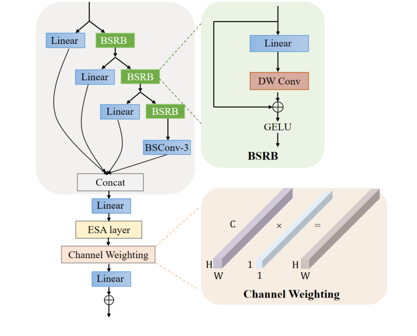
General method description. The XPixel team proposed Blueprint Separable Residual Network (BSRN) as shown in Fig. 8. Following the overall architecture of RFDN, BSRN consists of four stages including the shallow feature extraction, the deep feature extraction, multi-layer feature fusion, and reconstruction. In the first stage, the shallow feature extraction contains input replication followed by a linear mapping and a depthwise convolution to map from the input image space to a higher dimensional feature space. Then stacked efficient separable residual blocks (ESDB) build up the deep feature extraction to gradually refine the extracted features. Features generated by each ESDB are fused along the channel dimension at the end of the trunk. Finally, the SR image is produced by the reconstruction module, which only consists of a convolution and a non-parametric sub-pixel operation.
Building block description. For further optimization, the blueprint separable convolution is adopted, which is an extremely efficient decomposition of the convolution, to replace the regular convolution in the proposed blueprint separable residual block (BSRB), as shown in Fig. 9. RFDN replaces the contrast-aware channel attention (CCA) layer with the enhanced spatial attention (ESA) block for better performance. Yet, it has been found that the channel-wise feature rescaling is effective for shallow SR models to boost reconstruction accuracy. Therefore, a channel weighting layer is involved in each ESDB for modelling channel-wise relationships to utilize inter-dependencies among channels with slightly additional cost.
Model Details. The proposed BSRN model contains 5 ESDBs. the overall framework follows the pipeline of RFDN. A global feature aggregation is employed at the end of the network body to aggregate the final features, which is set to 48. Correspondingly, the channel weighting matrix is set to to match the dimension, which is initialized by normal distribution with , .
Training strategy. Data augmentation including random rotation by 90∘, 180∘, 270∘ and horizontal flipping is performed on the DIV2K and Flickr2K training images. In each training batch, 72 LR color patches with the size of are extracted as inputs per GPU. The model is trained by ADAM optimizor with . The initial leaning rate is set to equipped with cosine learning rate decay. Different from the recent SR models, loss is used for training from scratch for iterations. The model is implemented by Pytorch 1.9.1 and trained with 4 GeForce RTX 2080ti GPUs.
4.5 NJUST_ESR
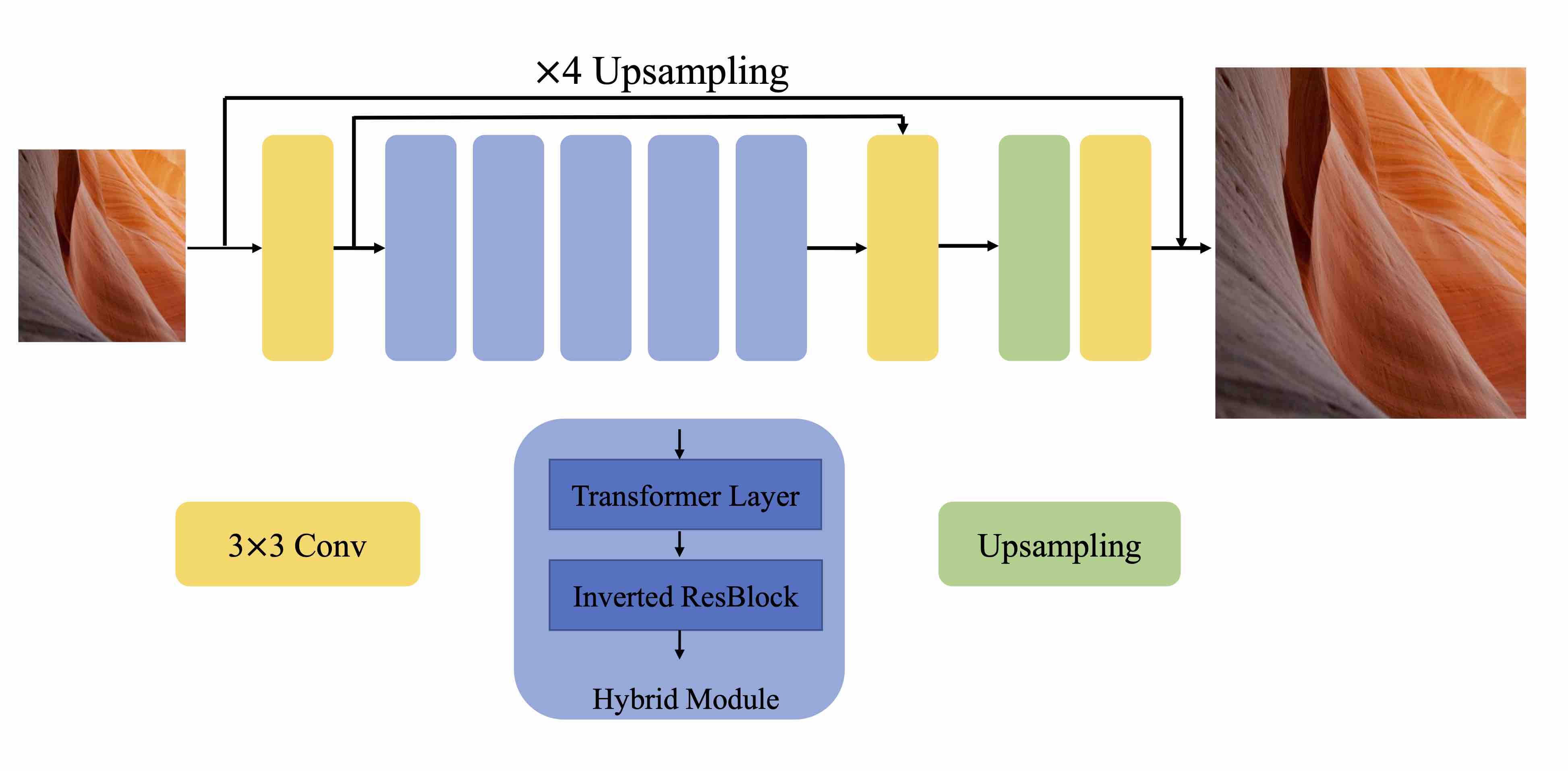
The NJUST_ESR introduced a vision transformer (ViT) based method for efficient SR, which combines the merits of convolution and multi-head self-attention. Specifically, a hybrid module containing a ViT block [38] and a inverted residual block [65] is employed to simultaneously extract local and global information. This module is stacked multiple times to learn discriminative feature representation.
The network consists of three stages as detailed in Fig. 10. First, a convolution layer maps the input image to feature space. Then five hybrid blocks are stacked to learn discriminative feature representation. At last, there are several convolution layers and pixel shuffle layers to generate the HR image.
The proposed MobileSR model is trained on DIV2K dataset. The input patches of size 6464 are randomly cropped from LR images, and the mini-batch size is set to 64. MobileSR is trained by minimizing L1 loss and the frequency loss[10] with Adam optimizer. The initial learning rate is set to and halved at every 100 epochs for total 450 epochs.
4.6 HiImageTeam
The HiImageTeam team proposed Asymmetric Residual Feature Distillation Network (ARFDN) inspired by the IMDN [31] and RFDN [51] for efficient SR. IMDN [31] is an efficient network architecture for image SR. Yet, there are still many redundant calculation and inefficient operators as shown in LABEL:fig:HiImageTeam_ARFDNa. Compared with IMDB, RFDB has a significant efficiency improvement in the calculation as shown in LABEL:fig:HiImageTeam_ARFDNb. A shallow residual block (SRB) in RFDN is equivalent to a normal convolution with sufficient training. The equivalent architecture of RFDB is shown in LABEL:fig:HiImageTeam_ARFDNc. That is to say, there is also redundant calculation in RFDN. An efficient attention module, namely ESA module is used in the enhancement stage of distillation information of RFANet [52]. Therefore, this module is also used in the proposed network. As shown in LABEL:fig:HiImageTeam_ARFDNd, an asymmetric residual feature distillation block is designed, which consists of both the asymmetric information distillation and the information recombination and utilization operation.
There are 4 ARFDBs in the proposed ARFDN, the overall framework follows the pipeline of RFDN [51], where global feature aggregation is used to augment the final feature and the number of feature channels is set to 50. HR patches are set to 256 256 and randomly cropped from HR images during the training of ARFDN. The mini-batch size is set to 36. The overall training process is divided into two stages. In the first stage, the ARFDN model is trained for 1000 epochs by minimizing L1 loss function with Adam optimizer and the initial learning rate is set to and halved at every 30 epochs. L2 loss function is used to fine-tune the network with learning rate of in the second stage. Div2K, OST and Flickr2K datasets are used to train the ARFDN model.




4.7 rainbow
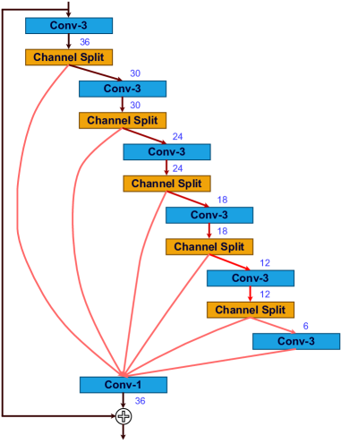
The rainbow team proposed Improved Information Distillation Network for efficient SR shown in Fig. 12. This solution mainly concentrates on improving the effectiveness of the information multi-distillation block (IMDB) [31]. Different from the original IMDB, as illustrated in Fig. 14, the improved IMDB (IMDB+) uses channel split operations. The number of input channels is set to . In order to improve the performance of IMDB+, structural re-parameterization methods are used [13, 85] to replace “Conv-3” during the training phase as shown in Fig. 13. Although re-parameterization can improve performance (about 0.03dB on DIV2K validation set), it will increase the training time. Different from the ECB proposed in ECBSR [85], Conv11-Sobel and Conv11-Laplacian are removed for efficient training. This is because Sobel and Laplacian filters are implemented by depth-wise convolution.
4.8 Super
The Super team proposed a solution mainly based on RFDN [51], where the channel splitting operation in IMDB [31] is replaced by convolution for feature distillation. The method differs from RFDN in three aspects: 1) Pixel Attention [90] is introduced in the network to effectively improve the feature representation capacity. 2) Model re-parameterization technique is adopted to expand the capacity of the network during training, while keeping the computations during inference. 3) Further compression of the model is accomplished by reducing the size of the first three blocks.
Framework. The team used a similar framework as RFDN [51], as shown in Fig. 15. The Pixel Attention Feature Distillation Network (RePAFDN) consists of four parts: the feature extraction convolution, the stacked feature distillation blocks with different sizes (FDB-S and FDB), the feature fusion part and the reconstruction block.
Given the input , coarse features are first extracted as:
| (3) |
where denotes the feature extraction function, implemented by a convolution, and is the extracted features. Next, three FDB-S and one FDB are stacked to gradually refine the extracted features, formulated as:
| (4) |
where denotes the -th feature distillation block, and represent the input feature and output feature of the -th feature distillation block, respectively. All the intermediate features are fused by a convolution and a convolution. The fused features are then fed to the pixel attention layer as:
| (5) |
where is the concatenation operation along the channel dimension, denots the convolution followed by a convolution, is the pixel attention layer, and is the fused features. Finally, the output is generated as:
| (6) |
where is the reconstruction function (i.e. a convolution and a sub-pixel operation) and is the output SR image.
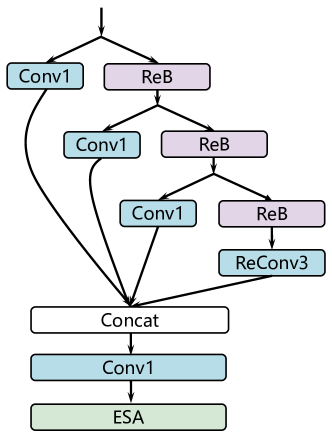
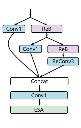
Feature Distillation Block. Two variants of Feature Distillation Block (FDB) are designed. The primitive FDB (Fig. 16(a)) is similar to RFDB except that the residual connection is removed and Re-parameterized Block (ReB) is used to replace the Shallow Residual Block (SRB). As shown in Fig. 16(c), ReB contains a re-parameterized convolution (ReConv3) and LReLU function. The details of the ReConv3 will be explained in the next paragraph. The whole structure of FDB can be described as:
| (7) | ||||
where is the -th convolution and is the -th ReB. The distilled features are concatenated and fed to a convlution and the ESA block [52] for further enhancement. As for the more lightweight FDB (FDB-S), a feature distillation layer (i.e. a convolution and a ReB) is removed as shown in Fig. 16(b).
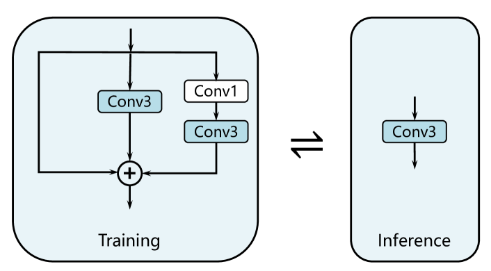

Model Re-parameterization. Inspired by recent model re-parameterization works [6, 85], similar techniques are adopted to improve model performance. Specifically, the SRB block inside RFDB is redesigned by introducing multi-branch convolution during training. As shown in Fig. 17, there are two extra branches along with the original convolution of size , which consists of an identity shortcut and two cascaded convolution layers with size of and respectively. The outputs of the three branches are added before being fed into the activation layer, which can be formulated as:
| (8) | ||||
where represents the input feature, and represents re-parameterized convolution. Since the operations of the three branches are completely linear, the re-parameterized architecture can be equally converted to a single convolution of size for inference. In the experiments, the re-parameterization technique helps improve the PSNR of small models by 0.02dB.
Pixel Attention. Inspired by PAN [90], pixel attention is used to more effectively generates features for the final reconstruction block. Specifically, a convolution followed by a Sigmoid function is responsible for generating a 3D attention coefficients map for all pixels of the feature map (shown in Fig. 18). The PA layer can be formulated as:
| (9) |
Unlike PAN, PA is not introduced into FDBs since PA is not runtime friendly. For similar consideration, the PA is conducted in low-resolution space to save computations while PA in UPA of PAN is conducted in higher resolution.
The channel number used in the model is . For in FDB, the number of output channels is . For and in FDB-S, the number of output channels is . DIV2K and Flickr2K are used as the training set. For the first training stage, patches of size are cropped from the LR images as inputs. For the second training stage, patches of size are cropped from the LR images as inputs.
4.9 MegSR
The MegSR team proposed PFDNet, a light-weight network for efficient super-resolution. Previous works such as IMDN [31] and RFDN [51] introduce novel network blocks, which are variants of feature distillation block, and achieve favorable performance. Unlike these works, the team proposed to tackle this problem based on pruning strategies. Albeit the techniques of network pruning are widely used in high-level tasks, such as image classification and segmentation, its applications on low-level tasks are rare. A recent work ASSL [89] propose a pruning scheme for residual network in the SR task, showing the network pruning technique is effective. Inspired by RFDN and ASSL, the team explored how to combine pruning and feature distillation network.
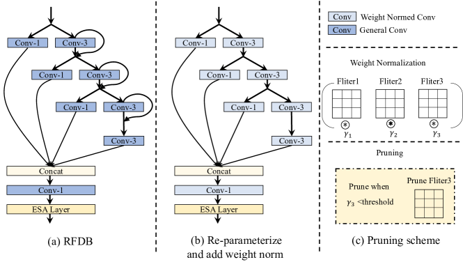
Specifically, the method contains two stages: training stage and fine-tuning stage. Training stage: In this stage, the original architecture of RFDN is first trained to obtain a pretrained model. Then, the model is reparameterized to reduce the residual addition operators as many as possible. When pruning the features of a network, the indices of features retained in different layers may be different. Thus, it is not reasonable to add up the features with different indices. To solve this problem, except for the ESA [52] layers, weight normalization (WN) is applied to all convolutions. The learnable parameters of WN indicate the importance of features. Finally, the new model is trained with loss to maintain the performance, while a regularized term is used to force the unimportant weights to converge to zero. Fine-tuning stage: After the training stage, the weights in the model is pruned according to the values of parameters . Note that, the remaining convolutional layers where are WN is not applied are pruned according to of the previous layers. The parameter can be fused into network weight during inference. Thus, using WN does not increase the computational cost. After pruning, the pruned model is fine-tuned with loss in the first iterations and with in the last iterations.
Reparameterization. Denote a feature as , and a weight of convolution as , this following equation holds:
| (10) |
where is the identity matrix. As depicted in Fig. 19(b), all the skip-connections are removed from RFDB without degradation.
Weight Normalization. Weight Normalization includes learnable parameters which can tell the importance of weights, as shown in Fig. 19 (c):
| (11) |
where represents the 4 dimensional convolutional kernel, and stands for the 1 dimensional trainable scale parameters in WN.
Loss Function. During training, the model is trained with loss and the following penalty term:
| (12) |
where is the scalar loss weight, denotes the i-th element of , and represents the unimportant filter index set in the l-th layer.
4.10 VMCL_Taobao
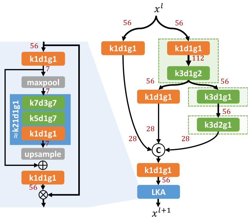

To improve the representation capacity of information flows in IMDN, the VMCL_Taobao team proposed a Multi-Scale information Distillation Network (MSDN) for efficient super-resolution, which stacks a group of multi-scale information distillation blocks (MSDB). Particularly, inspired by RFDN, a convolution is used for information distillation and a convolution is used for feature refinement to alleviate the limitation of channel splitting operation in IMDB. As shown in Fig. 20, in MSDB, a multi-scale feature refinement module (marked with green dotted boxes) is used to replace the convolution of RFDB. In Fig. 20, an upsampling refinement module with the scale factor of 2 is designed. A convolution is used for channel expansion and a convolution with two groups is used for feature refinement, which has receptive field to capture a larger region of neighbors and acts equivalently on an upsampled feature. Then, a single convolution is used for identical refinement as done in RFDB. Last, a dilated convolution with dilation rate of 2 is employed for downsampling refinement, which has receptive field and acts equivalently on a downsampled feature. By applying the multi-scale feature refinement, multi-scale information of the input features can be captured with fewer computations. Moreover, the Large Kernel Attention (LKA) [24] is introduced to enhance the features by capturing a larger receptive field.
4.11 Bilibili AI
The Bilibili AI team used Re-parameterized Residual Feature Distillation Network (Rep-RFDN) as shown in Fig. 21. Different from the original RFDN [51], all convolutional layers except those in the ESA block [51]) are replaced by RepBlocks (RB) in the training stage. During inference stage, the RepBlocks are converted into single convolutional layers. Inspried by ECB [85] and ACB [12], Conv and Conv sub-branches are added into the original ECB (Fig. 22). The number of feature channels is set to 40, while in the original RFDN50 version it is set to 50.
4.12 NKU-ESR
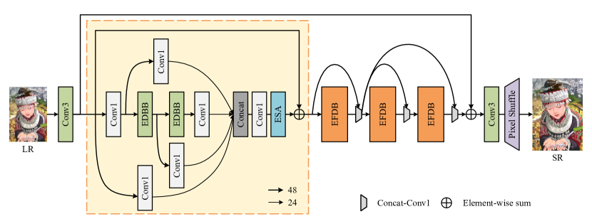
Generally, the team proposed an edge-enhanced feature distillation network, named EFDN, to preserve the high-frequency information under the synergy of network and loss devising. In detail, an edge-enhanced convolution block is built by revisiting the existing reparameterization methods. The backbone of the EFDN is searched by neural architecture search (NAS) to improve the basis performance. Meanwhile, an edge-enhanced gradient loss is proposed to calibrate the reparameterized block training.
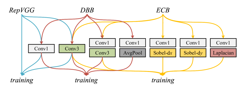

Edge-enhanced diverse branch block. As shown in Fig. 23(a), the detail of RepVGG Block, DBB, and ECB is presented. A total of eight different structures have been designed to improve the feature extraction ability of the vanilla convolution in different scenarios. Although the performance may be higher with more re-parameterizable branches, the expensive training cost is unaffordable for straightly integrating these paths. Meanwhile, another problem is that edge and structure information may be attenuated during the merging of parallel branches.
To address the above concerns, a more delicate and effective reparameterization block is built, namely Edge-enhanced Diverse Branch Block (EDBB), which can extract and preserve high-level structural information for the low-level task. As illustrated in Fig. 23(b), the EDBB consists of seven branches of single convolutions and sequential convolutions.
Network architecture. Following IMDN[31] and RFDN[51], an EFDN is devised to reconstruct high-quality SR images with sharp edges and clear structure under restricted resources. As illustrated in Fig. 24, the EFDN consists of an shallow feature extraction module, multiple edge-enhanced feature distillation blocks (EFDBs), and upscaling module. Specifically, a single vanilla convolution is leveraged to generate the initial feature maps.
This coarse feature is then sent to stacked EFDBs for further information refining. In detail, the shallow residual block in [51] is replaced by the proposed EDBB to construct the EFDB. Different from IMDN and RFDN utilizing global distillation connections to process input features progressively, neural architecture search (NAS) [30] is adopted to decide the feature connection paths. The searched structure is shown in the orange dashed box. Finally, the SR images are generated by upscaling module.
Edge-enhanced gradient-variance loss. In previous work[48], and loss have been in common usage to obtain higher evaluation indicators. The network trained with these loss functions often leads to the loss of structural information. Although the edge-oriented components are added into the EDBB, it is hard to ensure their effectiveness during the complex training procedure of seven parallel branches. Inspired by the gradient variance (GV) loss [1], an edge-enhanced gradient-variance (EG) loss is proposed, which utilizes the filters of the EDBB to monitor the optimization of the model. In detail, the HR image and SR image are transfered to gray-scale images and . The Sobel and Laplacian filters are leveraged to compute the gradient maps and then unfold gradient maps into patches , , . The -th variance maps can be formulated as:
| (13) |
where is the mean value of the -th patch. Thus, the variance metrics ,, of HR and SR images can be calculated, respectively. Referring to GV-loss, the gradient variance loss of different filter can be obtained by:
| (14) | ||||
Besides, is added to accelerate convergence and improve the restoration performance. In order to better optimize the edge-oriented branches of EDBBs and preserve sharp edges for visual effects, coefficients , , and are traded off, which are related to the scaled parameters of corresponding branches. The sum of the loss function can be expressed by:
| (15) |
4.13 NJUST_RESTORARION
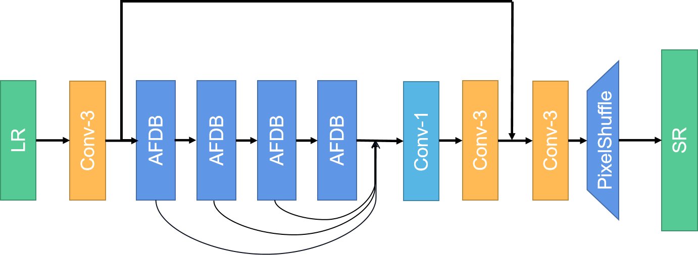
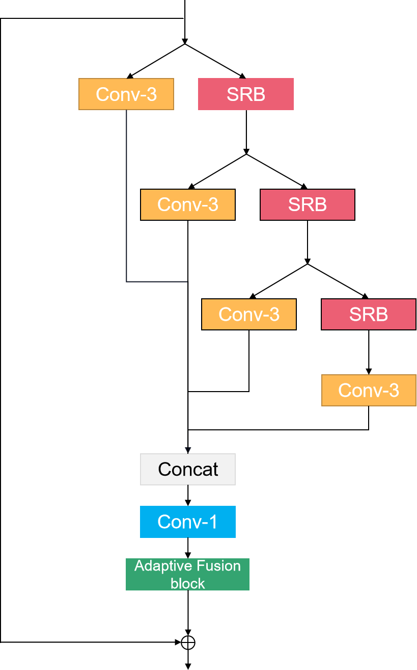
The NJUST_RESTORARION team proposed Adaptive Feature Distillation Network(AFDN) for lightweight image SR. The proposed AFDN shown in Fig. 25 is modified from RFDN [51] with minor improvements. AFDN uses 4 AFDBs as the building blocks, and the overall framework follows the pipeline of RFDN.
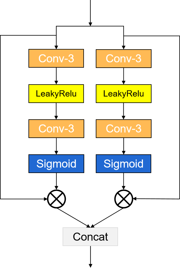
As illustrated in Fig. 25, AFDN uses Adaptive Fusion Block (AFB) which is more efficient to fuse features. AFB splits the feature in half. Each branch uses “Conv_3-LeakyRelu-Conv_3” to learn the adaptive attention matrix. Then AFB multiplies the feature with the attention matrix. Finally, it concatenates the features of two branches.
4.14 TOVBU
Method details. On the basis of Residual Feature Distillation Network, the team proposed a novel efficient Faster Residual Feature Distillation Network (FasterRFDN) for single image super resolution. The overall framework of the proposed method is shown in Fig. 27 and Fig. 28. The overall framework contains 4 faster residual feature distillation blocks (FRFDB). First, to further reduce the parameters and computational complexity of the FRFDB module, the number of channels of layered distillation is effectively compressed. The number of channels in each layer from top to bottom is 64, 32, 16, 16, respectively. These distillation features are extracted by three and one convolutional filters. Then, these features are fed to enhanced spatial attention (ESA) by concatenation along the channel dimension. Furthermore, in order to enhance the model’s representation power, the number of channels of the model is increased to 64.

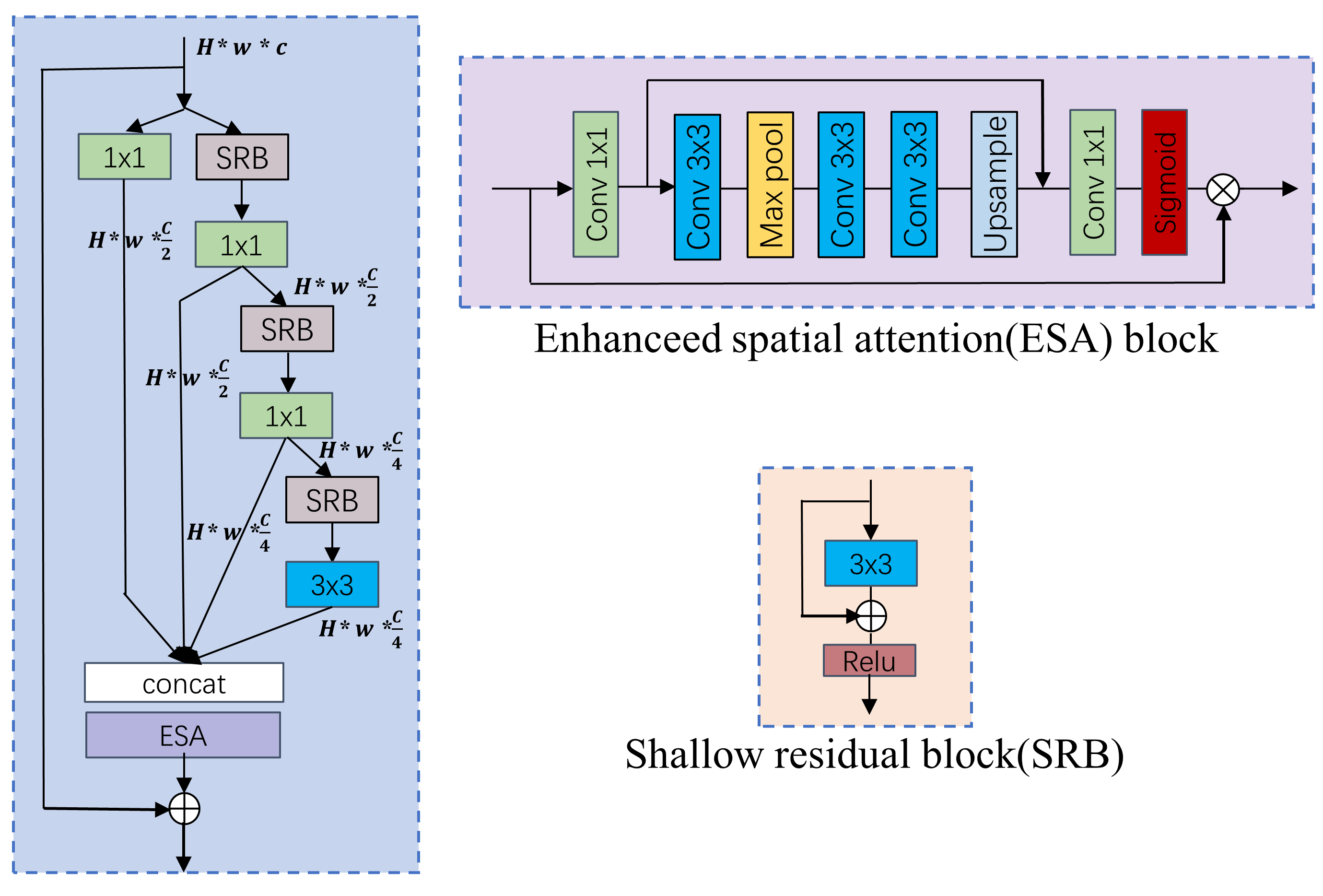
Training strategy. The training procedure can be divided into three stages.
-
1.
Pretraining on DIV2K and Flickr2K (DF2K). HR patches of size are randomly cropped from HR images, and the mini-batch size is set to 64. The model is trained by minimizing L1 loss function with Adam optimizer. The initial learning rate is set to and halved at every 200k iterations. The total number of iterations is 1,600k.
-
2.
Finetuning on DF2K. HR patch size is , and the mini-batch size are set to 64, respectively. The model is fine-tuned by minimizing PSNR loss function. The initial learning rate is set to and halved at every 80k iterations. The total number of iterations is 480k.
-
3.
Fine-tuning on DF2K again. HR patch size and the mini-batch size are set to and 16, respectively. The model is fine-tuned by minimizing L2 loss function. The initial learning rate is set to and cosine learning rate is used.
4.15 Alpan
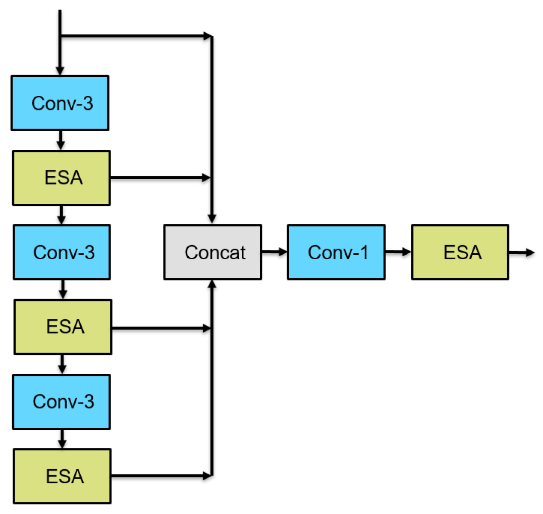
The Alpan team proposed the method based on RFDN [51] according to the following steps: 1) Rethinking of RFDB[51]. 2)Efficiency and PSNR trade-off for ESA[51] block and convolution. 3) Fine-tuning width and depth.
The team’s first observation is that ESA [51] block was efficient and significantly improves the results. Thus, the team placed ESA block after each convolution in RFDB [51]. All distillation convolutions from RFDB [51] (three convolutions and one convolution) are removed and the number of RFDB[51] blocks is reduced from to to keep the same inference time. All these changes have the following effect: 1) PSNR goes up from to on DIV2K validation set. 2) The number of parameters is reduced from M to M. 3) FLOPS is reduced from G to G.
The team’s next observation was that in the modified RFDB % parameters and more than % FLOPS belonged to convolutions outside of ESA [51] blocks. So the team decided to re-balance the number of channels in ESA block. Specifically, the overall number of channels in the model is reduced from to but the number of channels in ESA blocks is increased from to . All these changes have the following effect: 1) PSNR is almost the same on DIV2K validation set. 2) The number of parameters is reduced from M to M. 3) FLOPS is reduced from G to G.
In most of the team’s experiments deeper models are better than wider models with the same efficiency. So the team decided to reduce the overall number of channels from to while keeping channels in ESA blocks and to increase the number of modified RFDB blocks from to . This leads to significant reduction in FLOPS and small reduction in parameters in the final model: 1) Number of parameters: M. 2) FLOPS: G
The final model SR_model consists of modified RFDB blocks with channels. All the other unmentioned parts of the model are the same as in RFDN. The modified RFDB block is shown in Fig. 29.
4.16 xilinxSR
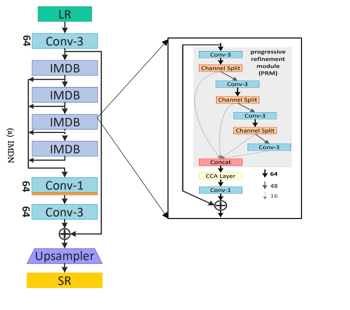


The overview of IMDN is illustrated in Fig. 30. It is a lightweight information multi-distillation network composed of the cascaded information multi-distillation blocks (IMDB). Specifically, it adopts a series of IMDB blocks (default 8) and a traditional upsampling layer (pixelshuffle) for high-resolution image restoration.
Network Pruning. Based on IMDN, network pruning is firstly performed. Tab. 2 provides models of different sizes and the corresponding accuracy. To achieve a trade-off between accuracy and runtime, the number of IMDB blocks is reduced from 8 to 7 as the baseline.
| Method | #IMDB | Params | PSNR |
| target | 29.00dB | ||
| IMDN | 8 | 0.8939M | 29.13dB |
| IMDN | 7 | 0.7905M | 28.97dB |
| IMDN | 6 | 0.6871M | 28.93dB |
| IMDN | 5 | 0.5836M | 28.91dB |
| IMDN | 4 | 0.4802M | 28.85dB |
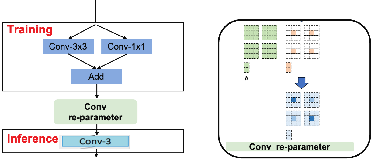
Collapsible Block. Inspired by SESR [6], the team applied a collapsible block to improve the pruned IMDN accuracy. Specifically, as shown in Fig. 31, a dense block is adopted to enhance the representation during training. Each convolution in IMDB is replaced by a convolution and a convolution. These two convolutions are conducted in parallel and the outputs are summed. During inference, the two parallel convolutions are converted to one convolution.
Training strategy. The network was trained on DIV2K with Flick2K as the extra dataset. The training patch size is progressively increased from to to improve the performance. The batch size is 32 and the number of epochs is 500. The network is trained by minimizing L1 loss with Adam optimizer and a dynamic learning rate ranging from to . Data augmentation, like rotation and horizontal flip, is applied.
4.17 cipher
The cipher team proposed an end-to-end residual distillation network (ResDN) for lightweight image SR. As shown in Fig. 32, the proposed ResDN consists of three parts: the head, trunk and tail parts.
The trunk part consists of four ResDBs and one BFM. After the coarse features is obtained, the four ResDBs will extract intermediate features in turn, namely
| (16) |
where denotes the function of the -th ResDB, and represents the intermediate features extracted by the -th ResDB.
As shown in Fig. 32, the will be aggregated into BFM and the feature dimensions is first halved by convolution followed by the ReLU activation function (omitted in Fig. 32), and then sequential concatenations are utilized. This can be formulated as
| (17) |
where and denote the concatenation operation along the channel dimension and convolution, respectively. By the sequential fusion, different hierarchical features can be used more fully. Finally, the coarse features will be transmitted by a residual connection to generate the deep features .
As shown in Fig. 33, the body of ResDB is stacked by several residual blocks (RBs). Here, there is a PReLU activation function in front of each convolution layer, and a learnable parameter is set for each channel in PReLU. In RB, convolution is first used to expand the channel dimension for the convenience of distillation. Suppose there are RBs in total and the input of the -th RB is with channels, and the number of distilled feature channel is . In RB, the intermediate feature obtained by convolution can be expressed as
| (18) |
where denotes the PReLU activation function. denotes the convolution with convolutional kernels. Then, the intermediate features are split along the channel axis, and each distilled features with channels flow to the latter RBs. And the retained features with channels flow to the convolution for further refinement. Moreover, at the beginning of each residual branch, the distilled features are concatenated on the previous residual branches of RBs and the input feature of current RB. Finally, ESA and a skip connection are used to generate the output features of ResDB.
4.18 NJU_MCG


Inspired by WDSR [80], the residual feature expansion block (RFEB) in Fig. 34(a) is used as the basic unit of the feature distillation and expansion network (FDEN). FDEN adopts the architecture of RFDN [51] except that the basic unit is replaced by RFEB and the attention mechanism is replaced by the LapSA module in Fig. 34(c). The LapSA module is responsible for applying the scale transformation for each spatial position of the input features. To achieve this goal, it needs to have a global assessment to assign different scaling factors for different positions according to the spatial importance. Specifically, for the task of image super-resolution, the network should concentrate more on the high-frequency regions that are usually difficult to recover because of the complex details. As a consequence, the LapSA module is implemented to contain a Laplacian pyramid (Fig. 34(b)) which has a large receptive field and can extract the high-frequency details as well. This process can be formulated as
| (19) | ||||
As depicted in Fig. 34(b), denotes the downsampling function that consists of a pooling layer and a convolutional layer. is the interpolation function that upsamples the input feature. , and are the output features of the three pyramid levels, respectively. The extracted feature contains high-frequency information and is used in the LapSA module (Fig. 34(c)) to generate the scaling factors.
As shown in Fig. 34(c), the first convolution is used to reduce the channel dimension and the last convolution is used to recover the channel dimension. The middle convolution is used to aggregate the pyramid features and then the sigmoid function is applied to generate the final scaling factors. is concatenated with the scaled features to augment the output features as
| (20) | ||||
The number of filters () in FDEN is set to 29. The proposed FDEN is trained with the same training setting as RFDN. DIV2K and Flickr2K datasets are adopted as the training dataset.

4.19 IMGWLH
The IMGWLH team proposed RLCSR network. The overall network structure is shown in Fig. 35. A convolutional layer is firstly used to extract shallow features from low-resolution images. Then six Local residual feature fusion block (RFDB+) modules are then stacked to perform deep feature extraction on the shallow features. RFDB+ is an improved version of RFDB [51]. Without increasing the number of parameters of the ESA module, more skip connections are included to ensure better retention of useful information and use dilated convolution to expand the receptive field for preserving more texture details.
In order to produce compact features, a CCM model is introduced to fuse the intermediate features from several RFDB+. The module is developed based on MBFF module [58] and the backward fusion model [57]. The detailed structure of CCM is illustrated in Fig. 37. It can be observed that different levels of features from several RFDB+ are gradually fused to a single feature map using our proposed CCM. The channel shuffle operation and convolution kernel can integrate the features of all basic residual blocks, which helps to extract more contextual information in a compact manner.
To further enhance the intermediate features produced by RFDB+, LAM [59] module is used to introduce an attention mechanism for adaptively selecting representative features from multiple intermediate features. One can refer to Fig. 36 for the structure of LAM.
However, the collected features could still be full of redundancy. To address the issue, a weight is assigned to the feature map through the Hadamard multiplication of channel attention and pixel attention. To produce features for high-resolution reconstruction, a long-term skip connection is included, with which the deep features are added to the shallow features that are extracted at the beginning of the network.

4.20 imgwhl

The imgwhl team proposed a lightweight SR network named RFESR to achieve a compact network design and fast inference speed. To be specific, the work is based on the structure of IMDB [31] and inspired by several advanced techniques [58, 52].
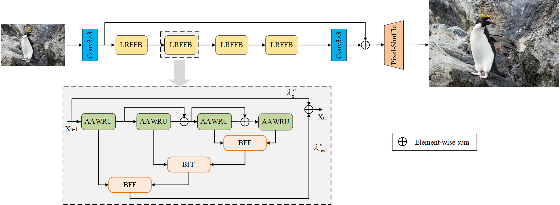
The proposed network is shown in Fig. 38. A convolution is first used to extract shallow features from inputs. Then, four Local residual feature fusion block (LRFFB) modules are stacked to perform deep feature extraction on the shallow features. After gradual feature refinement by the LRFFBs, another convolution is used to extract final deep features from the output of the last LRFFN module. The final deep and shallow features are element-wise added through a long-range skip connection. Finally, the high-resolution images can be reconstructed through a pixel Shuffle block that consists of a convolution and a non-parametric sub-pixel operation.
The two building blocks are presented as follows.
LRFFB. Each LRFFB module contains four basic residual units, i.e. , Attention-guided Adaptive Weighted Residual Unit (AAWRU). Inspired by the MBFF module [58], the backward feature fusion (BFF) module is introduced to fuse multi-level features acquired from AAWRUs. The feature extracted by AAWRU of LRFFB is denoted by . For example, the feature extracted by the second AAWRU in the first LRFFB is . Specifically, in the LRFFB, the last two features ( and ) are aggregated by a BFF module. The structure of the BFF module is shown in Fig. 39(c). It first concatenates the two input features and then processes the aggregated features by a channel shuffle operation [86] and convolution kernel. The BFF module is repeated three times until all level features are fused in an LRFFB. The input features are then added to the output fused feature in an element-wise manner. As residue may contain redundant information, the results are multiplied with trainable parameters to select useful information.
AAWRU. The detailed structure of the AAWRU module is shown in Fig. 39(a). Inspired by the residual block proposed in the RFANet [52], MAFFSRN [58] introduced an enhanced fast spatial attention module (EFSA). It aims to realize spatial attention weighting to make the features more concentrated in some desired regions, so that more representative features can be obtained. The two branches of the residual structure in AAWRU are assigned by adaptive weights, which help more shallow-level features be activated without increasing parameters. The design of the EFSA module is shown in Fig. 39(b). Using the blocks above, the proposed model can better extract and integrate compact contextual information with fewer parameters, which helps produce more delicate SR images.
4.21 whu_sigma
The team designed their method based on RFDN [51]. They simply used dilated convolution to replace the convolution part in the RFDB module and adjusted the number of channel of RFDN to 64.

4.22 Aselsan Research
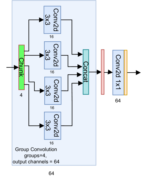
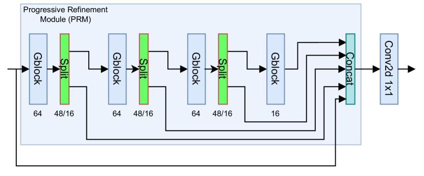
The team created a network structure where progressive refinement module (PRM) is repeated locally in the blocks and globally among the blocks to reduce the number of parameters. This is done in a way that intermediate information collection (IIC) modules in the global setting is replaced with proposed Global PRM. Furthermore, block based non-local attention block [73] is employed in the main path of the network while is avoided in the individual IMDB blocks. To further reduce the number of parameters and number of operations of the network, every single convolution operation inside the IMDB is replaced with Gblocks (Fig. 41) as in XLSR [5] which is based on group convolution. The group convolution based structures is referred to as Grouped Information Distilling Blocks (GIDB). Yet, grouped convolutions are unfortunately not well optimized in PyTorch framework [21]. If implemented properly within an inference oriented framework, group convolutions can lead to speedups [5, 21] especially in mobile devices where efficient network structures are usually employed.
4.23 Drinktea
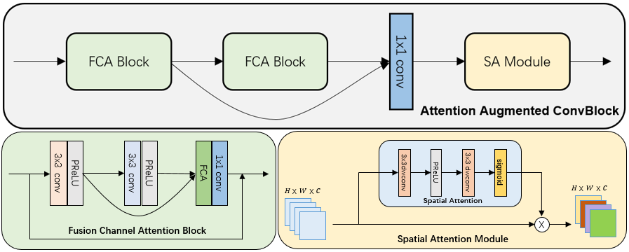
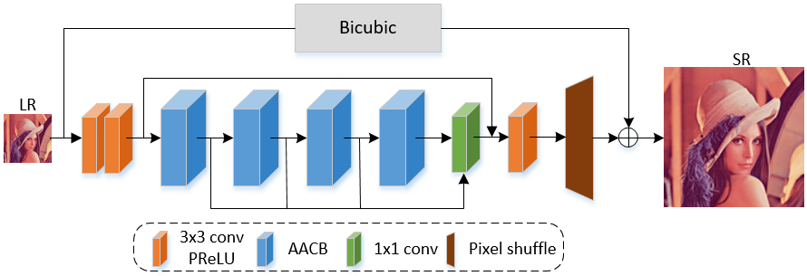
Inspired by IMDN and LatticeNet [57], the Drinktea team proposed a method to obtain channel attention which can effectively utilize the mean and the standard deviation of feature maps. First, as shown in Fig. 43, the mean value is calculated by global average pooling and the standard deviation of each feature map is also computed. Second, the statistic vector in each branch is passed to a convolution layer which performs channel-downscaling with reduction ratio and then activated by ReLU. Third, the two vectors are added up to fuse the information extracted by each vector. Then the fusion vector is restored to the original number of channels. Finally, the sigmoid activation is utilized to weight the vector to generate channel attention. FCAB utilizes the features from different hierarchical and augments them with channel attention [77].
Spatial attention can effectively improve the performance of the model, but it is difficult to achieve a balance between complexity and performance in lightweight network. Inspired by ULSAM [64], the team designed a spatial attention module for super-resolution task. As shown in Fig. 44, the features on each channel is first extracted with depthwise convolution and activated with PReLU function. Then another depthwise convolution and sigmoid function are applied to redistribute the weights. As shown in Fig. 44, the basic the Attention Augmented ConvBlock (AACB) is composed of two FCABs, a convolution and a spatial attention module. The architecture of attention augmented lightweight network (AALN) for efficient image SR is shown in Fig. 45.
4.24 GDUT_SR
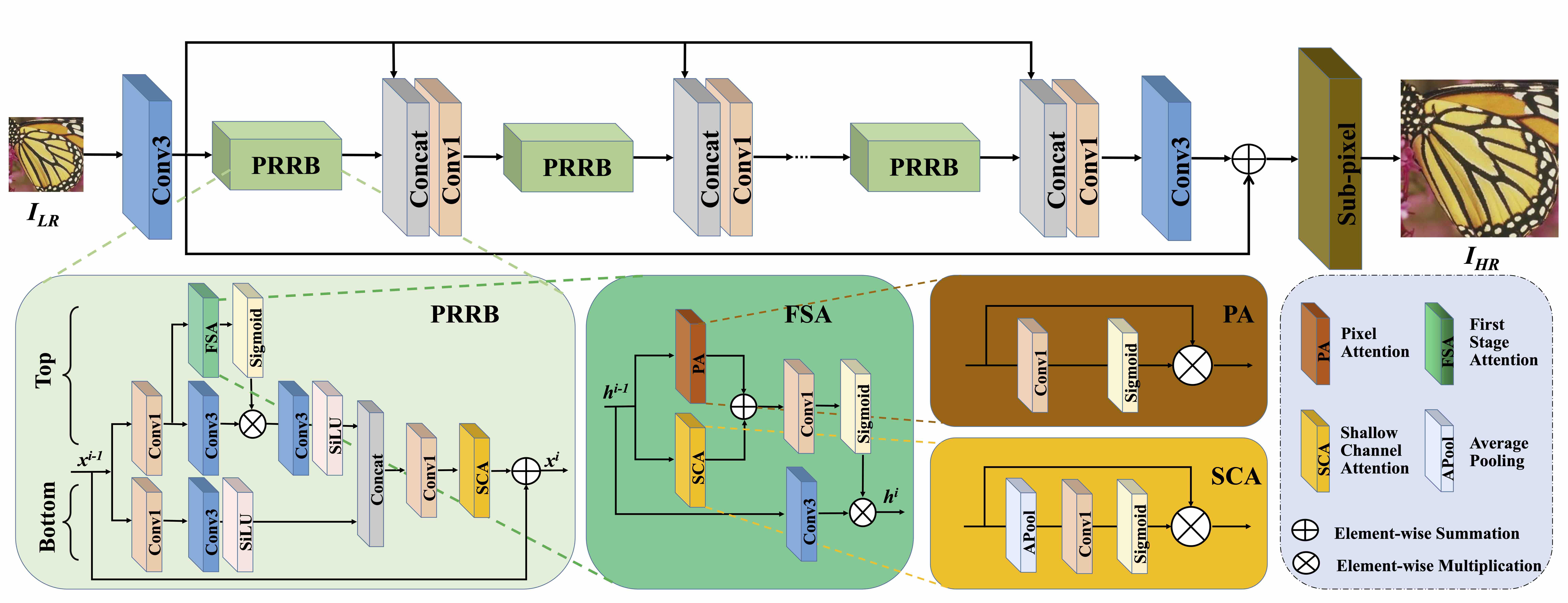
The GDUT_SR proposed Progressive Representation Re-Calibration Network (PRRN) for lightweight SR. The proposed PRRN shown in Fig. 46 is modified from PAN [90] but achieves better performance and runtime efficiency than PAN with limited increase of parameters. The main contribution of PRRN is to adjust the receptive field of CNN by using the pixel and channel information in a two-stage manner. A shallow channel attention (SCA) mechanism is proposed to build the correspondences between channels in a simpler yet more efficient way. The architecture of PRRN can be divided into three components: shallow feature extractor, deep feature extractor, and reconstruction. The shallow feature is extracted by using convolution layer, while the deep feature extractor is stacked by the proposed Progressive Representation Re-calibration Blocks (PRRBs). Finally, the pixel shuffle layer is used to reconstruct the HR image.
The deep feature extractor consists of 16 PRRBs and multiple long skip connections are applied to propagate the initial features to the intermediate layers. PRRB precisely explores the discriminative information in a two-stage manner. In the first stage, the First Stage Attention (FSA) uses pixel attention (PA) [90] to capture important pixel information and the proposed SCA mechanism is applied to learn useful channel information. Therefore, the first stage of PRRB can explore the spatial and channel information simultaneously. In the second stage, an SCA modified from squeeze-and-excitation (SE) [29] is used to further rescale the importance of the output feature channels. SCA uses average pooling to collect channel information and then uses convolution and sigmoid activation function to process the information. Moreover, inspired by the recent work [49], SiLU activation is used at the end of both the top and bottom branches of FSA.
Giantpandacv
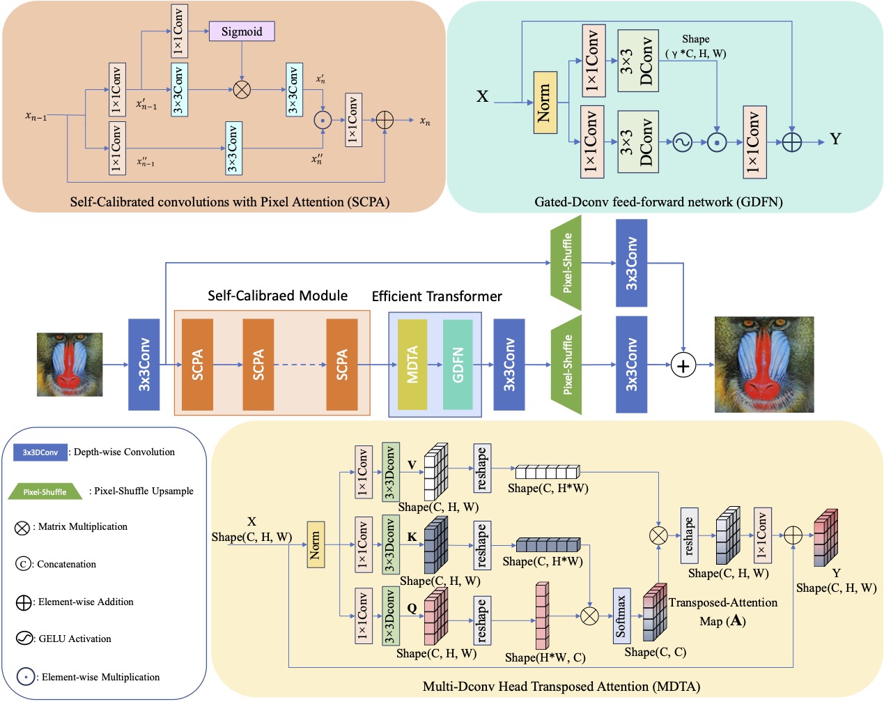
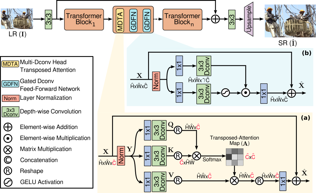
The Giantpandacv team proposed a lightweight Self-Calibrated Efficient Transformer (SCET) network, which is inspired PAN [90] and Restormer [81]. The architecture of SCET mainly consists of the Self-Calibrated module and Efficient Transformer block, where the Self-Calibrated module adopts the pixel attention mechanism to extract image features effectively. To further exploit the contextual information from features, an efficient Transformer module is employed to help the network obtain similar features over long distances and thus recover sufficient texture details.
The main architecture of the network is shown in Fig. 47, which consists of the Self-Calibrated module and the Efficient Transformer block. The details of these modules of SCET are described as follows.
Self-Calibrated module. In this module, 16 cascaded Self-Calibrated convolutions with Pixel Attention (SCPA) blocks are utilized for a larger receptive field. The SCPA block [90] consists of two branches. One of the branches is equipped with a pixel attention module to perform the attention mechanism in the spatial dimension while the other branch is used to retain the original high-frequency feature information. Furthermore, skip connection is utilize to facilitate network training.
Efficient Transformer. The efficient transformer block is utilized to further exploit the contextual information from features to obtain useful contextual information. In the efficient transformer block, Multi-Dconv Head Transposed Attention (MDTA) is used to avoid the vast computational complexity of the traditional self-attention mechanism. And a feed-forward network is further employed with a gating mechanism to recover precise texture details.
4.25 TeamInception
The proposed solution is based on the Transformer-based architecture Restormer that is recently introduced in [81]. Specifically, an isotropic version of Restormer is built, which operates at the original resolution and does not contain any downsampling operation.
Overall pipeline. The overall pipeline of the Restormer architecture is presented in Fig. 48. Given a low-resolution image , Restormer first applies a convolution to obtain low-level feature embeddings ; where denotes the spatial dimension and is the number of channels. Next, these shallow features pass through multiple transformer blocks (six in this work) and transformed into deep features , to which shallow features are added via skip connection. Finally, a convolution layer followed by pixel shuffle layer is applied to the deep features to generate residual high-resolution image , where denotes the scaling factor. To obtain the final super-resolved image, the residual image is added the bilinearly upsampled input image as: .
In the proposed Transformer block, the core components are: (a) multi-Dconv head transposed attention (MDTA) and (b) gated-Dconv feed-forward network (GDFN).
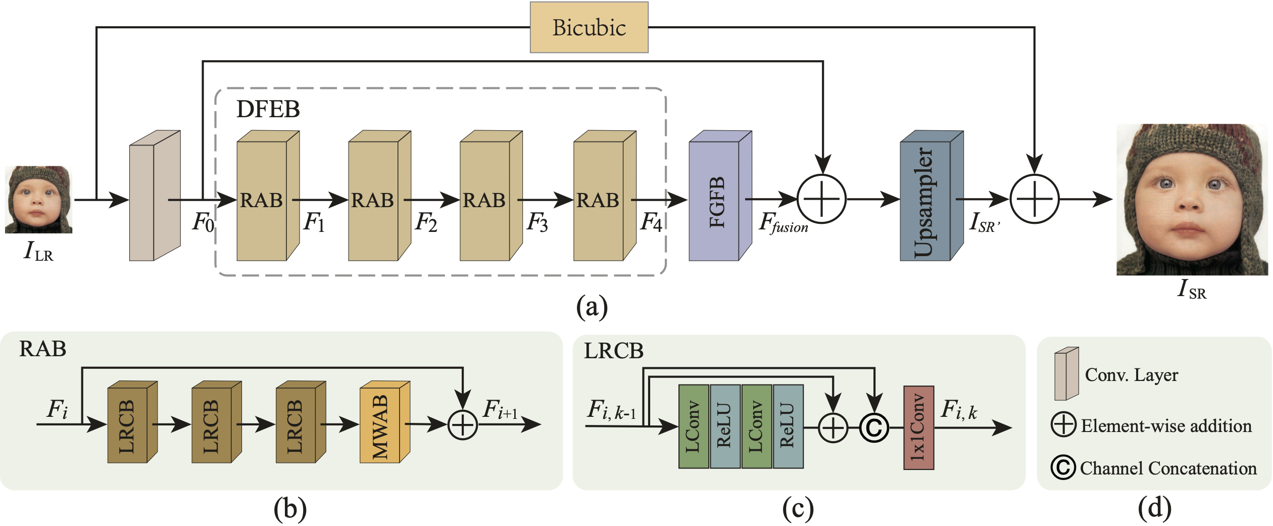
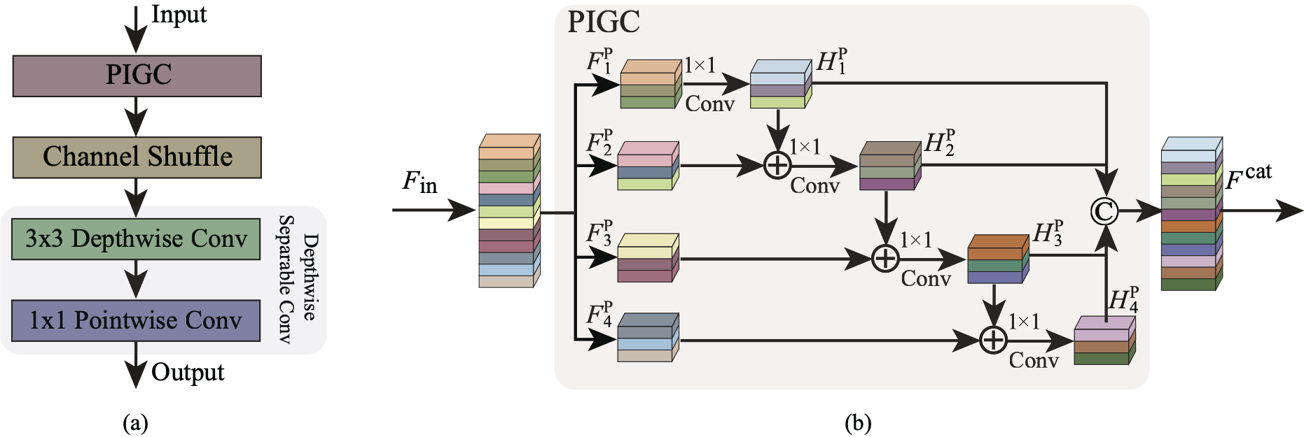
Multi-Dconv Head Transposed Attention. The major computational overhead in Transformers comes from the self-attention layer, which has quadratic time and memory complexity. Therefore, it is infeasible to apply SA on most image restoration tasks that often involve high-resolution images. To alleviate this issue, MDTA is proposed. The key ingredient is to apply SA across channels rather than the spatial dimension, i.e. , to compute cross-covariance across channels to generate an attention map encoding the non-local context implicitly. As another essential component in MDTA, depth-wise convolutions is introduced to emphasize on the local context before computing feature covariance to produce the global attention map [45].
Gated-Dconv Feed-Forward Network. A feed-forward network (FN) is the other building block of the Transformer model [17], which consists of two fully connected layers with a non-linearity in between. As shown in Fig. 48(b), the first linear transformation layer of the regular FN [17] is reformulated with a gating mechanism to improve the information flow through the network. This gating layer is designed as the element-wise product of two linear projection layers, one of which is activated with the GELU non-linearity. Our GDFN is also based on local content mixing similar to the MDTA module to equally emphasize on the spatial context, which is useful for learning local image structure for effective restoration. The gating mechanism in GDFN controls which complementary features should flow forward and allows subsequent layers in the network to specifically focus on more refined image attributes, thus leading to high-quality outputs. Progressive learning is performed where the network is trained on smaller image patches in the early epochs and on gradually larger patches in the later training epochs. The model trained on mixed-size patches via progressive learning shows enhanced performance at test time where images can be of different resolutions (a common case in image restoration).
4.26 cceNBgdd
The VLESR network architecture shown in Fig. 49 (a), mainly consists of a 33 convolutional layer, a deep feature extraction block (DFEB), a frequency grouping fusion block (FGFB), and an Upsampler. DFEB contains four residual attention blocks (RABs), and Upsampler uses subpixel convolution.
Each RAB contains three lightweight residual concatenation blocks (LRCBs), a multi-way attention block (MWAB), and a skip connection, as shown in Fig. 49 (b). The LRCB consists of two parts, as shown in Fig. 49 (c). The first part contains two lightweight convolutional blocks (LConv) (see Section 3.3), two ReLU nonlinear activation layers immediately following each LConv and a skip connection to learn the local residual feature information. The learned residual features are concatenated with the original feature to enhance the utilization and propagation of the feature information. In the second part, a 11 convolutional layer is used to compress the concatenated feature. The multi-way attention block (MWAB) is shown in Fig. 51. The MWAB contains three branches, where the first and the second branches focus on the global information, and the third branch focuses on the local information. The three branches explore the clues of different feature information respectively and sum the calculated importance (i.e. , weights) of each channel.
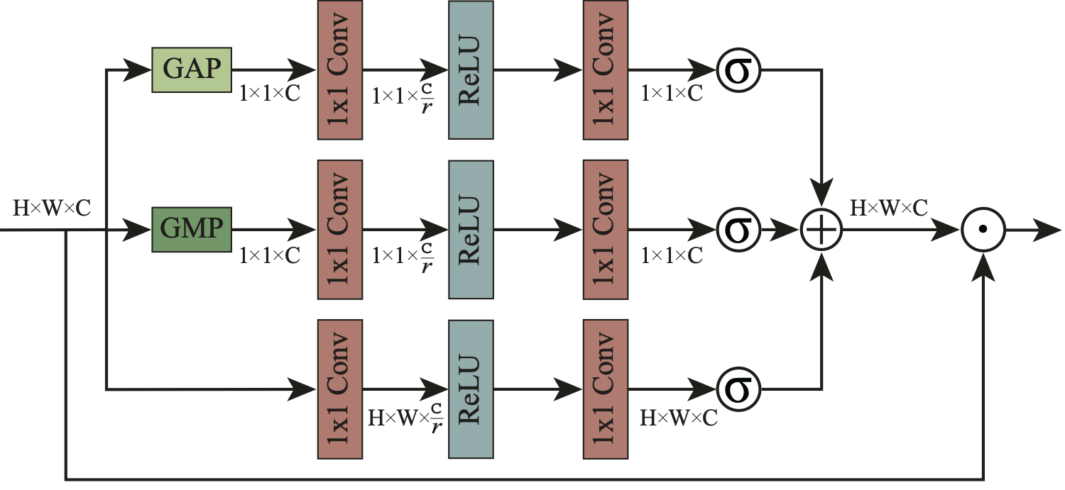
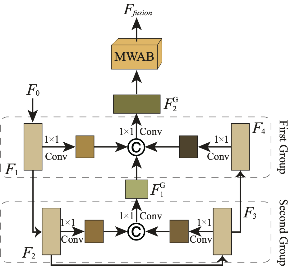
Based on the ShuffleNet [86], a very lightweight building block is designed for the SISR task, called the lightweight convolutional block (LConv). The important improvements are twofold: (1) Remove the batch normalization layers from the ShuffleNet unit, which have been shown to deteriorate the accuracy of SISR; (2) In ShuffleNet unit, the first 11 group convolution is replaced with the progressive interactive group convolution (PIGC), and the second 11 group convolution is replaced with the 11 point-wise convolution to enhance the interaction between the group features. The structure of the LConv is shown in Fig. 50 (a), which consists of a PIGC, a channel shuffle layer, a 33 depth-wise convolution, and a 11 point-wise convolution. The structure of the PIGC in the LConv is shown in Fig. 50 (b).
The frequency grouping fusion block (FGFB) is shown in Fig. 52. The features with the highest difference between low-frequencies and high-frequencies are divided into the first group, the features with the next highest difference are divided into the second group, and so on. Then, starting from the feature group with the smallest frequency difference, the features of each group are gradually fused until the feature group with the largest frequency difference. If the number of the RABs is odd, only the output feature of the middle RAB is used as the last feature group. The output feature by grouping fusion is then fed into the MWAB for the further fusion. When the number of the RABs is 4, there are only two feature groups.
4.27 ZLZ
The team proposed to use Information Multi-distillation Transformer Block (IMDTB) in Fig. 53 as the basic block, where the convolution in IMDB[31, 32] was converted to grouped convolution and the number of groups is 4. The channel shuffling operation is used [86] to increase the information interaction between channels. The attention mechanism is replaced with a Swin-Transformer[54, 47] to better deal with images spatial relations with attention mechanism.
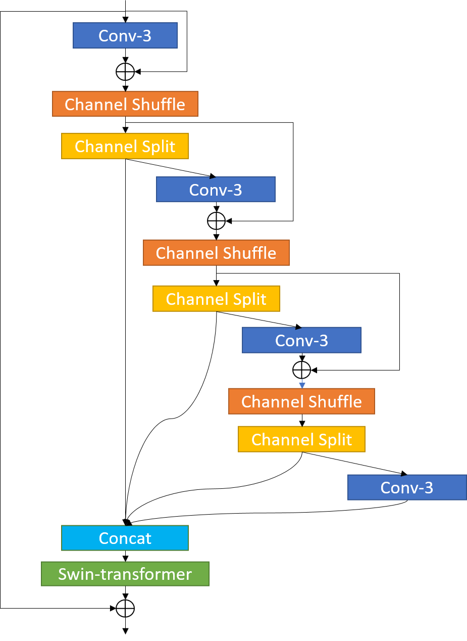
4.28 Express
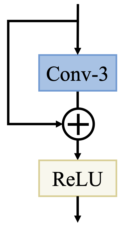 |
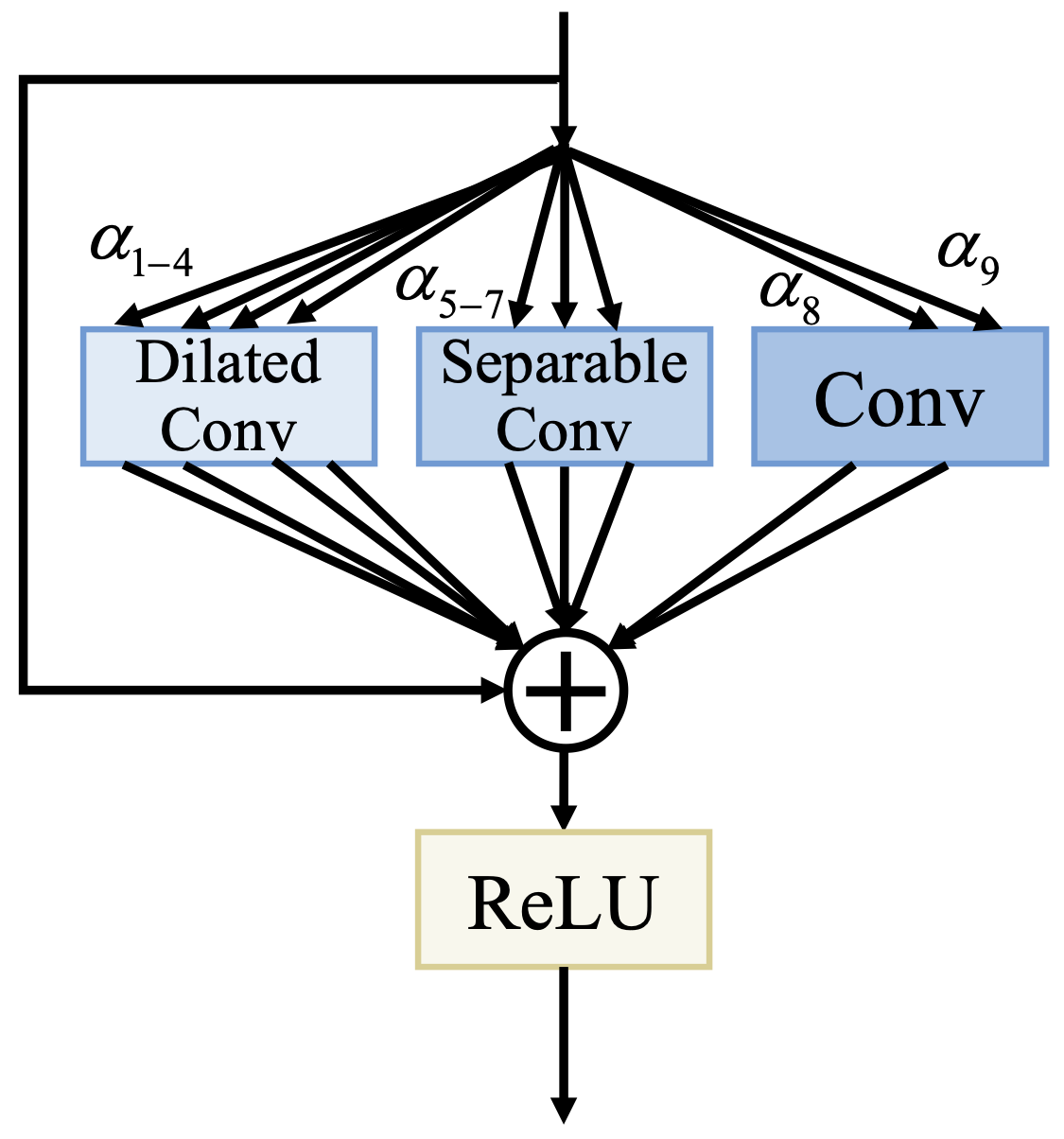 |
| (a) Shallow residual block (SRB) | (b) Mixed operations block (Mixed OP) |
Existing lightweight SR methods such as IMDN [31] and RFDN [51] have achieved promising performance with a great equilibrium between performance and parameters or inference speed. However, there is still room for improvement in their network architectures. For instance, the convolution kernels have been widely adopted by IMDN [31] and RFDN [51], while its optimality is still questionable. Blocks based on the convolution kernels may be suboptimal for lightweight SISR tasks. Neural network architecture search (NAS) may be served as an ideal approach. Inspired by DARTS [50] and DLSR [30], the proposed solution is based on DARTS [50] and DLSR [30], which is a fully differentiable NAS method for lightweight SR model. The aim is to find the lightweight network for efficient SR by searching the best replacement of convolution kernels of shallow residual block in RFDB. Next, the search space, search strategy and the searched network are introduced in sequence.
| Operation | Kernel Size | Params (K) | Muti-Adds (G) |
| convolution | 2.5 | 0.576 | |
| 22.5 | 5.184 | ||
| 62.5 | 14.400 | ||
| 122.5 | 28.224 | ||
| Separable convolution | 5.9 | 1.359 | |
| 7.5 | 1.728 | ||
| 9.9 | 2.281 | ||
| Dilated convolution | 2.95 | 0.680 | |
| 3.75 | 0.864 |
Search space. Based on residual feature distillation block of (RFDB)[51], the smallest building block, i.e. shallow residual blocks (SRB) consist of a convolution layer and a residual connection as shown in Fig. 54(a). In order to search for a more lightweight structure with competitive performance, the convolution layer is replaced with a mixed layer as shown in Fig. 54(b). The mixed layer is composed of multiple operations including separable convolution, dilated convolution, and normal convolution as shown in Tab. 3. The input is denoted as , and the operation set is denoted as where each element represents a candidate operation that is weighted by the architecture parameters . Then, like DARTS [50], softmax function is used to perform the continuous relaxation of the operation space. Thus, the output of mixed layer denoted by is given as:
| (21) |
After searching, only the operation with the largest is reserved as the best choice of this layer. All three SRBs of each RFDB will be replaced by the searched results. The search space contains different structures. The network structure and its corresponding cell structure during searching is shown in Fig. 55 (a) and Fig. 55 (b), respectively.
 |
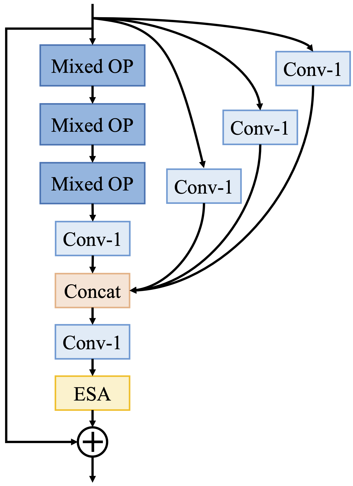 |
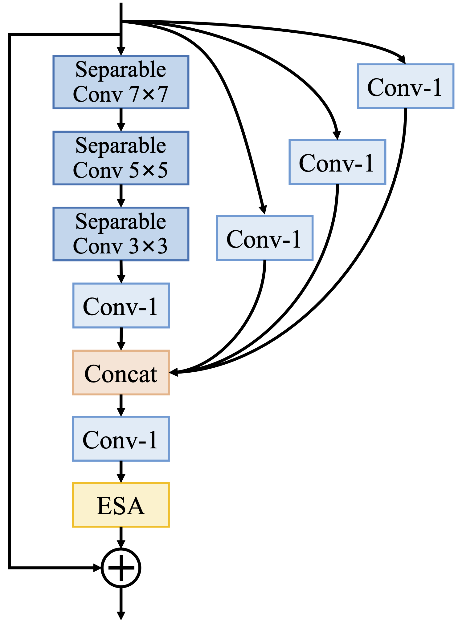 |
| (a) The network structure | (b) The cell structure during searching | (c) The searched cell structure |
Search strategy. The differentiable NAS method is applied to the lightweight SISR task. The objective function of the model is defined as
| (22) |
where denotes the weights parameters of the network, and is a non-negative regularization parameter that balances the importance of the training loss and validation loss. Since the architecture parameter is continuous, Adam[36] is directly applied to solve problem (2). The parameters , are updated are updated with subsequent iterations:
| (23) |
| (24) |
The searching and training procedure is summarized in Algorithm 1.
Searched results. As shown in Fig. 55 (c), the searched cell is composed of a separable convolution layer, separable convolution layer, separable convolution layer, ESA block, and residual connections with information distillation mechanism. Since the number of parameters and FLOPs of the searched results are all fewer than the original convolution layer, a much smaller (nearly half the original size) model is obtained compared with RFDN [51].
Loss function. To achieve lightweight and accurate SR models, the loss function is the weighted sum of these three losses:
| (25) |
| (26) |
| (27) |
| (28) |
Specifically, [9] is a gradient-domain loss and can improve image details; denotes the number of parameters of operation and utilizes them to weigh the architecture parameter , so as to push the algorithm to search for lightweight operations. The and are weighting parameters that balance the reconstruction performance and model complexity, respectively. When retraining the searched network, set and remove the last item in the total loss function Eq. 28.
4.29 Just Try
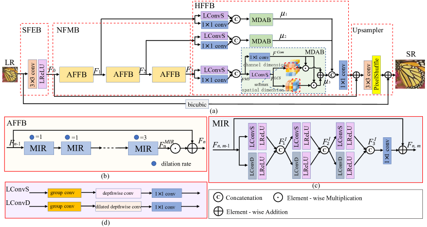
The team designed a multi-branch network structure LWFANet, The LWFANet extracts the shallow feature with one convolution layer. The extracted feature is sent to the deep feature extraction module which consists of 10 LWFA blocks and a convolution layer. Each LWFA block has four branches, every branch consists of a convolution layer and several convolution layers. The convolutional layer selects the input features and reduces the number of channels to one-fourth of the input channels, the different number of convolutional layers are used to extract the features at different levels. Then multi-level features of every branch are concatenated and used the channel attention mechanism for adaptive aggregation of features . Then spatial attention is used to get . The input feature is also enhanced by spatial attention, leading to . The final output of the LWFA block is obtained sum up , and . Long skip connections are used to get the final output feature. Then convolution layer is used to reduce the dimension. The upsampling module consists of nearest interpolation and convolution layers. The reconstructed image is derived after two convolution operations.
4.30 ncepu_explorers
The ncepu_explorers team proposed the MDAN network architecture shown in Fig. 56, consists of four main parts: shallow feature extraction block (SFEB), nonlinear feature mapping block (NFMB), hierarchical feature fusion block (HFFB), and upsampling block (Upsampler). The SFEB consists of only one 3 3 convolutional layer and one leaky rectified linear unit (LReLU), and the Upsampler uses the sub-pixel convolution. The NFMB cascades ( = 3) area feature fusion blocks (AFFBs). The HFFB mainly consists of multiple pairs of the lightweight convolutional units (LConvSs) / 1 1 convolutions and multiple multi-dimensional attention blocks (MDABs).
In the MDAN architecture, three AFFBs were cascaded in the NFMB, and the number of input and output channels for each AFFB was 48. Six MIRs were cascaded in each AFFB, and the dilation rates of the dilation convolutions in each MIR were set to 1, 1, 2, 2, 3 and 3. In each MIR, the number of the input channels of both LConvS and LConvD was 48 and the number of the output channels was 24. The group convolutions in both LConvS and LConvD used three groups. The initial values of the learnable parameters , , and in the HFFB were set to 0.3, 0.3, and 0.4, respectively.
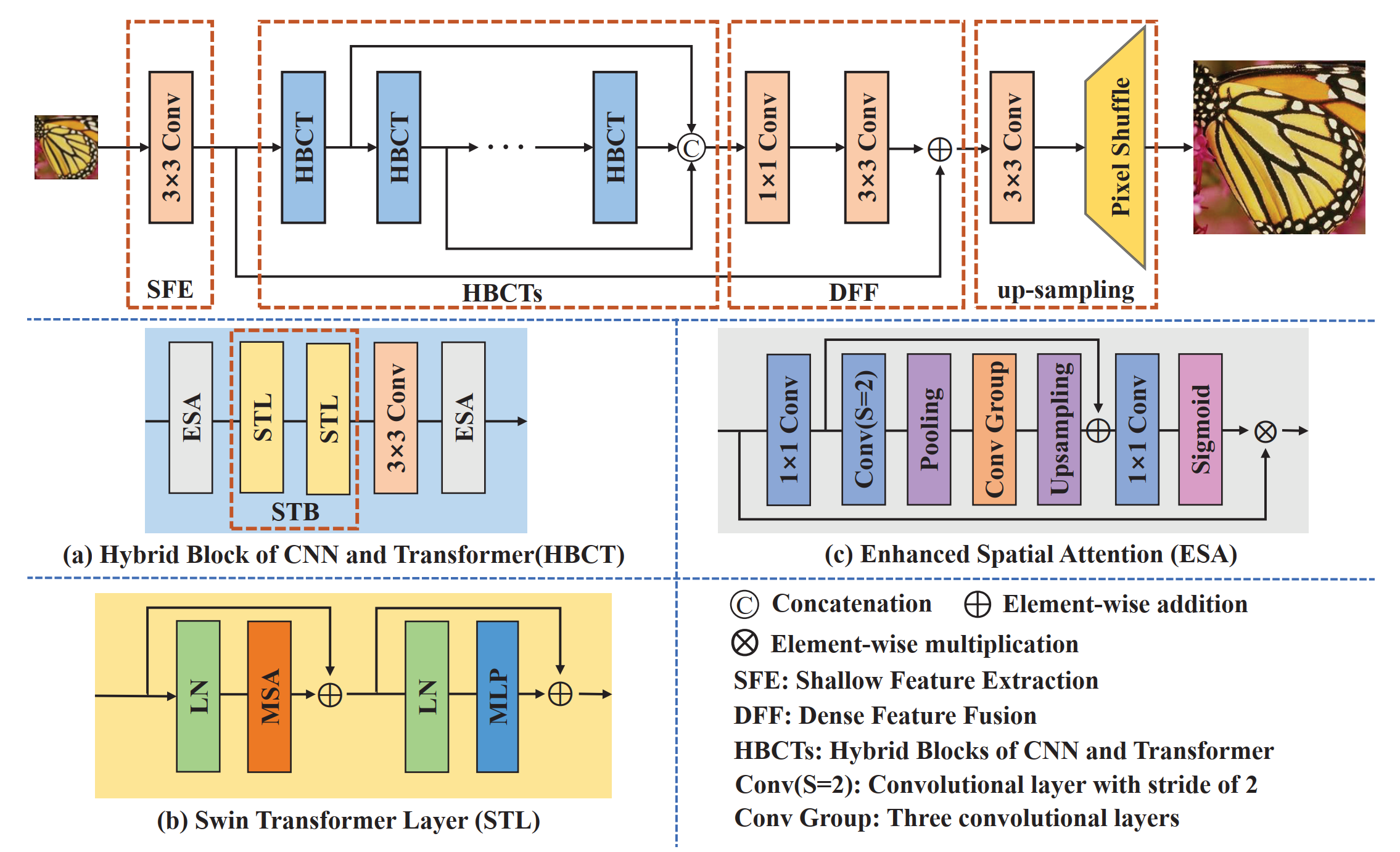
4.31 mju_mnu
The team proposed a lightweight SR model namely hybrid network of CNN and Transformer (HNCT) in Fig. 57, which integrated CNN and transformers to model local and non-local priors simultaneously. Specifically, HNCT consists of four parts: shallow feature extraction (SFE) module, Hybrid Blocks of CNN and Transformer (HBCTs), dense feature fusion (DFF) module and up-sampling module. Firstly, shallow features containing low-frequency information are extracted by only one convolution layer in the shallow feature extraction module. Then, four HBCTs are used to extract hierarchical features. Each HBCT contains a Swin Transformer block (STB) with two Swin Transformer layers inside, a convolutional layer and two enhanced spatial attention (ESA) modules. Afterwards, these hierarchical features produced by HBCTs are concatenated and fused to obtain residual features in SFE. Finally, SR results are generated in the up-sampling module. Integrating CNN and transformer, the HNCT is able to extract more effective features for SR.
Acknowledgments
We thank the NTIRE 2022 sponsors: Huawei, Reality Labs, Bending Spoons, MediaTek, OPPO, Oddity, Voyage81, ETH Zurich (Computer Vision Lab) and University of Wurzburg (CAIDAS).
Appendix A Teams and affiliations
NTIRE 2022 team
Title: NTIRE 2022 Efficient Super-Resolution Challenge
Members:
Yawei Li1 (yawei.li@vision.ee.ethz.ch),
Kai Zhang1 (kai.zhang@vision.ee.ethz.ch),
Luc Van Gool1 (vangool@vision.ee.ethz.ch),
Radu Timofte1,2 (radu.timofte@vision.ee.ethz.ch)
Affiliations:
1 Computer Vision Lab, ETH Zurich, Switzerland
2 University of Würzburg, Germany
ByteESR
Title: Residual Local Feature Network For Efficient Super-Resolution
Members:
Fangyuan Kong (kongfangyuan@bytedance.com),
Mingxi Li, Songwei Liu
Affiliations:
ByteDance, Shenzhen, China
NJU_Jet
Title: Fast and Memory-Efficient Network with Window Attention
Members:
Zongcai Du1 (151220022@smail.nju.edu.cn),
Ding Liu2
Affiliations:
1 State Key Laboratory for Novel Software Technology, Nanjing University, China
2 ByteDance Inc.
NEESR
Title: Edge-Oriented Feature Distillation Network for Lightweight Image Super Resolution
Members: Chenhui Zhou1 (daomujun@foxmail.com), Jingyi Chen1, Qingrui Han1
Affiliation:
1 NetEase, Inc.
XPixel
Title: Blueprint Separable Residual Network for Single Image Super-Resolution
Members:
Zheyuan Li1 (zy.li3@siat.ac.cn), Yingqi Liu1, Xiangyu Chen1,2, Haoming Cai1, Yu Qiao3,1, Chao Dong3,1
Affiliations:
1 Shenzhen Institutes of Advanced Technology, CAS
2 University of Macau
3 Shanghai AI Lab, Shanghai, China
NJUST_ESR
Title: MobileSR: A Mobile-friendly Transformer for Efficient Image Super-Resolution
Members:
Long Sun1 (cs.longsun@gmail.com), Jinshan Pan1, Yi Zhu2
Affiliations:
1 Nanjing University of Science and Technology
2 Amazon Web Services
HiImageTeam
Title: Asymmetric Residual Feature Distillation Network
Members:
Zhikai Zong (zzksdu@163.com), Xiaoxiao Liu
Affiliations:
Qingdao Hi-image Technologies Co.,Ltd (Hisense Visual Technology Co.,Ltd.)
rainbow
Title: Improved Information Distillation Network for Efficient Super-Resolution
Members: Zheng Hui
(huizheng.hz@alibaba-inc.com), Tao Yang, Peiran Ren, Xuansong Xie, Xian-Sheng Hua
Affiliation:
Alibaba DAMO Academy, EFC, Yuhang District, Hangzhou, Zhejiang, China
Super
Title: Re-parameterized Pixel Attention Feature Distillation Network
Members:
Yanbo Wang (51205901021@stu.ecnu.edu.cn), Xiaozhong Ji1,2, Chuming Lin2, Donghao Luo2, Ying Tai2, Chengjie Wang2,
Zhizhong Zhang1, Yuan Xie1
Affiliations:
1 East China Normal University
2 Youtu Lab, Tencent
MegSR
Title: Feature Distillation Network Pruning for Efficient Image Super-Resolution
Members: Shen Cheng1
(chengshen@megvii.com), Ziwei Luo1, Lei Yu1, Zhihong Wen1, Qi Wu1, Youwei Li1, Haoqiang Fan1, Jian Sun1 and Shuaicheng Liu2,1
Affiliation:
1 Megvii Technology
2 University of Electronic Science and Technology of China
VMCL_Taobao
Title: Multi-scale Information Distillation Network for Efficient Super-resolution
Members: Yuanfei Huang1
(yfhuang@bnu.edu.cn), Meiguang Jin2, Hua Huang1
Affiliation:
1 School of Artificial Intelligence, Beijing Normal University
2 Alibaba Group
Bilibili AI
Title: RepRFDN: Using Re-parameterization technology into lightweight image super resolution
Members:
Jing Liu (liujing04@bilibili.com), Xinjian Zhang
Affiliations:
Bilibili AI
NKU-ESR
Title: Edge-enhanced Feature Distillation Network for Efficient Super-Resolution
Members:
Yan Wang (wyrmy@foxmail.com)
Affiliations:
Nankai-Baidu Joint Lab, Nankai University, Tianjin, China
NJUST_RESTORATION
Title: Adaptive Feature Distillation Network for Lightweight Super-Resolution
Members:
Lingshun Kong (konglingshun@njust.edu.cn), Jinshan Pan
Affiliations:
Nanjing University of Science and Technology
TOVBU
Title: Faster Residual Feature Distillation Network for Efficient Super Resolution
Members:
Gen Li (leegeun@yonsei.ac.kr), Yuanfan Zhang, Zuowei
Cao, Lei Sun
Affiliations:
Platform Technologies, Tencent Online Video
Alpan
Members: Panaetov Alexander
(aapanaetov@edu.hse.ru)
Affiliation:
Higher School of Economics (@edu.hse.ru), Huawei Moscow Research Center (@huawei.com)
Dragon
Title: Double Branch Network With Enhanced Spatial Attention
Members: Yucong Wang
(1401121556@qq.com), Minjie Cai
Affiliation:
Hunan University
TieGuoDun Team
Title:
Members:
Shuhao Zhang (zhangshuha0@163.com), Yuhao Zhang
Affiliations:
Xidian University
xilinxSR
Title: Efficient Image Super-Resolution with Collapsible Linear Blocks
Members:
Li Wang (liwa@xilinx.com), Lu Tian
Affiliations:
Xilinx Technology Beijing Limited
cipher
Title: ResDN: Residual Distillation Network for Single Image Super-Resolution
Members: Zheyuan Wang1
(cipherwon@163.com), Hongbing Ma2
Affiliation:
1 College of Information Science and Engineering, Xinjiang University, Urumqi,China
2 Department of Electronic Engineering, Tsinghua University,
Beijing,China
NJU_MCG
Title: Feature Distillation and Expansion Network (FDEN)
Members:
Jie Liu (jieliu@smail.nju.edu.cn), Chao Chen, Yidong Cai, Jie Tang, Gangshan Wu
Affiliations:
Nanjing University
IMGWLH
Members: Weiran Wang1
(Wangweirantx@163.com), Shirui Huang, Honglei Lu, Huan Liu, Keyan Wang, Jun Chen
Affiliation:
Xidian University
McMaster University
imgwhl
Title: Residual Feature Extraction Super-Resolution
Members: Shirui Huang1
(shiruihh@gmail.com), Weiran Wang, Honglei Lu, Huan Liu, Keyan Wang, Jun Chen
Affiliation:
1 School of Telecommunication Engineering, Xidian University, Xi’an, China
2 McMaster University
whu_sigma
Title: Feature Distillation Network of Dilated Convolution for Lightweight Image Super-Resolution
Members:
Shi Chen1 (chenshi@whu.edu.cn), Yuchun Miao2, Zimo Huang3, Lefei Zhang1
Affiliations:
1 School of Computer Science, Wuhan University, Wuhan, China
2 School of Mathematical Science, University of Electronic Science and Technology of China, Chengdu, China
3 School of Computer Science, The University of Sydney, Sydney, Australia
Aselsan Research
Title: IMDeception: Grouped Information Distilling Super-Resolution Network
Members:
Mustafa Ayazoğlu (mayazoglu@aselsan.com.tr),
Affiliations:
Aselsan Research, Ankara, Turkey
Drinktea
Title: Attention Augmented lightweight network
Members:
Wei Xiong (scun2016@163.com), Chengyi Xiong, Fei Wang
Affiliations:
School of Electronic and Information Engineering, South-Central University for Nationalities, Wuhan, China
GDUT_SR
Title: Progressive Representation Re-Calibration Network for Lightweight
Super-Resolution
Members:
Hao Li (lihao9605@gmail.com), Ruimian Wen, Zhijing Yang
Affiliations:
Guangdong University of Technology
Giantpandacv
Members: Wenbin Zou
(alexzou14@foxmail.com), Weixin Zheng, Tian Ye, Yuncheng Zhang
Affiliation:
Fujian Normal University, Fuzhou University, Jimei University, China Design Group
neptune
Title:
Members:
Xiangzhen Kong (neptune.team.ai@gmail.com),
TeamInception
Title: Restormer: Efficient Transformer for Image Super-Resolution
Members: Aditya Arora1
(adityadvlp@gmail.com), Syed Waqas Zamir1, Salman Khan3, Munawar Hayat2, Fahad Shahbaz Khan3
Affiliation:
1 Inception Institute of Artificial Intelligence (IIAI), Abu Dhabi, UAE
2 Monash University, Melbourne, Australia
3 Mohamed bin Zayed University of AI
cceNBgdd
Title: A Very Lightweight and Efficient Image Super-Resolution Network
Members:
Dandan Gao (gdd@ncepu.edu.cn), Dengwen Zhou
Affiliations:
North China Electric Power University, Changping District, Beijing
Express
Title: Searching Lightweight Network for Efficient Super-resolution
Members:
Qian Ning (ningqian@stu.xidian.edu.cn), Jingzhu Tang, Han Huang, Yufei Wang, Zhangheng Peng
Affiliations:
The School of Artificial Intelligence of Xidian University
Just Try
Title: Light Weight Feature Aggregation for Image Super-Resolution
Members:
Haobo Li1 (qwerdf20191024@gmail.com), Wenxue Guan11, Shenghua Gong2, Xin Li1, Jun Liu1,2
Affiliations:
1 College of Computer Science and Technology, Jilin University
2 School of Electronic and Information Engineering, Beihang University
ncepu_explorers
Title: MDAN
Members:
Wanjun Wang (1206371055@qq.com), Dengwen Zhou
Affiliations:
School of Control and Computer Engineering, North China Electric Power University, Beijing, China
mju_mnu
Title: Hybrid network of CNN and Transformer for Lightweight Image Super-Resolution
Members:
Kun Zeng1 (zengkun301@aliyun.com), Hanjiang Lin2, Xinyu Chen; Jinsheng Fang
Affiliations:
1 Minnan Normal University, Zhangzhou, Fujian, China
2 Minjiang University, Fuzhou, Fujian, China
Virtual_Reality
Title: Non-Local Fourier Convolution for Efficient Image Super Resolution
Members:
Abhishek Kumar Sinha (aks@sac.isro.gov.in), S. Manthira Moorthi, Debajyoti Dhar
Affiliations:
Space Applications Centre, Ahmedabad
NTU607QCO-ESR
Title: Re-parameterized and pruned model for Efficient SR
Members:
Hao-Hsiang Yang1 (islike8399@gmail.com), Zhi-Kai Huang1, Wei-Ting Chen2, Hua-En Chang1, Sy-Yen Kuo1
Affiliations:
1 Department of Electrical Engineering, National Taiwan University, Taiwan
2 Graduate Institute of Electronics Engineering, National Taiwan University, Taiwan
Strong Tiger
Title: Multi-Directional Gradient Network for Real-time Super Resolution
Members:
Wei Tan (tanwei0699@163.com),
Affiliations:
DAMO Academy, Alibaba Group
VAP
Title: CL-RFDN: Collapsible Lightweight Residual Feature Distillation Network for Efficient Image Super-Resolution
Members: Hao Chen
(xu.qian5@zte.com.cn), Qian Xu
Affiliation:
ZTE, Nanjing, China
Multicog
Title: Modified Residual Feature Distillation Network
Members: Pratik Narang1
(pratik.narang@pilani.bits-pilani.ac.in), Usneek Singh1, Syed Sameen1, Harsh Khaitan2
Affiliation:
1 BITS Pilani, Pilani, Rajasthan
2 Kwikpic Tech. Services, Kolkata, India
Set5baby
Title: Self Residual Feature Distillation Network
Members: Liu Yinghua1
(727630081@qq.com), Zhang Tianlin2, Zhang Xiaoming3
Affiliation:
1 Computer Vision Institute, Shenzhen University, Shenzhen, China
2 CAS Key Laboratory of Electronic and Information Technology for Complex Aerospace Systems, National
Space Science Center, Chinese Academy of Science (CAS)
3
Institue of Artificial Intelligence, Southwest Jiaotong University
NWPU SweetDreamLab
Title: Branch Mixed Distillation Network for Efficient Super-Resolution
Members: Dingxuan Meng
(mdxgalaxy20@gmail.com), Chunwei Tian
Affiliation:
Northwestern Polytechnical University
SSL
Title: RFDNeXt
Members: Mashrur M. Morshed
(mashrurmorshed@iutdhaka.
edu), Ahmad Omar Ahsan
Affiliation:
Islamic University of Technology,
Dhaka, Bangladesh
References
- [1] Lusine Abrahamyan, Anh Minh Truong, Wilfried Philips, and Nikos Deligiannis. Gradient variance loss for structure-enhanced image super-resolution. arXiv preprint arXiv:2202.00997, 2022.
- [2] Eirikur Agustsson and Radu Timofte. NTIRE 2017 challenge on single image super-resolution: Dataset and study. In Proceedings of the IEEE Conference on Computer Vision and Pattern Recognition Workshops, pages 126–135, 2017.
- [3] Boaz Arad, Radu Timofte, Rony Yahel, Nimrod Morag, Amir Bernat, et al. NTIRE 2022 spectral demosaicing challenge and dataset. In Proceedings of the IEEE/CVF Conference on Computer Vision and Pattern Recognition (CVPR) Workshops, 2022.
- [4] Boaz Arad, Radu Timofte, Rony Yahel, Nimrod Morag, Amir Bernat, et al. NTIRE 2022 spectral recovery challenge and dataset. In Proceedings of the IEEE/CVF Conference on Computer Vision and Pattern Recognition (CVPR) Workshops, 2022.
- [5] Mustafa Ayazoglu. Extremely lightweight quantization robust real-time single-image super resolution for mobile devices. In Proceedings of the IEEE/CVF Conference on Computer Vision and Pattern Recognition, pages 2472–2479, 2021.
- [6] Kartikeya Bhardwaj, Milos Milosavljevic, Liam O’Neil, Dibakar Gope, Ramon Matas, Alex Chalfin, Naveen Suda, Lingchuan Meng, and Danny Loh. Collapsible linear blocks for super-efficient super resolution. arXiv preprint arXiv:2103.09404, 2021.
- [7] Goutam Bhat, Martin Danelljan, Radu Timofte, et al. NTIRE 2022 burst super-resolution challenge. In Proceedings of the IEEE/CVF Conference on Computer Vision and Pattern Recognition (CVPR) Workshops, 2022.
- [8] David Capel and Andrew Zisserman. Computer vision applied to super resolution. IEEE Signal Processing Magazine, 20(3):75–86, 2003.
- [9] Chakravarty R Alla Chaitanya, Anton S Kaplanyan, Christoph Schied, Marco Salvi, Aaron Lefohn, Derek Nowrouzezahrai, and Timo Aila. Interactive reconstruction of monte carlo image sequences using a recurrent denoising autoencoder. ACM Transactions on Graphics (TOG), 36(4):1–12, 2017.
- [10] Sung-Jin Cho, Seo-Won Ji, Jun-Pyo Hong, Seung-Won Jung, and Sung-Jea Ko. Rethinking coarse-to-fine approach in single image deblurring. In Proceedings of the IEEE/CVF International Conference on Computer Vision (ICCV), pages 4641–4650, October 2021.
- [11] Matthieu Courbariaux, Yoshua Bengio, and Jean-Pierre David. Binaryconnect: Training deep neural networks with binary weights during propagations. In Advances in Neural Information Processing Systems, pages 3123–3131, 2015.
- [12] Xiaohan Ding, Yuchen Guo, Guiguang Ding, and Jungong Han. Acnet: Strengthening the kernel skeletons for powerful cnn via asymmetric convolution blocks. In Proceedings of the IEEE/CVF international conference on computer vision, pages 1911–1920, 2019.
- [13] Xiaohan Ding, Xiangyu Zhang, Jungong Han, and Guiguang Ding. Diverse branch block: Building a convolution as an inception-like unit. In Proceedings of the IEEE/CVF Conference on Computer Vision and Pattern Recognition, pages 10886–10895, 2021.
- [14] Xiaohan Ding, Xiangyu Zhang, Ningning Ma, Jungong Han, Guiguang Ding, and Jian Sun. Repvgg: Making vgg-style convnets great again. In Proceedings of the IEEE/CVF Conference on Computer Vision and Pattern Recognition, pages 13733–13742, 2021.
- [15] Chao Dong, Chen Change Loy, Kaiming He, and Xiaoou Tang. Learning a deep convolutional network for image super-resolution. In Proceeding of the European Conference on Computer Vision, pages 184–199. Springer, 2014.
- [16] Chao Dong, Chen Change Loy, and Xiaoou Tang. Accelerating the super-resolution convolutional neural network. In Proceeding of the European Conference on Computer Vision, pages 391–407. Springer, 2016.
- [17] Alexey Dosovitskiy, Lucas Beyer, Alexander Kolesnikov, Dirk Weissenborn, Xiaohua Zhai, Thomas Unterthiner, Mostafa Dehghani, Matthias Minderer, Georg Heigold, Sylvain Gelly, et al. An image is worth words: Transformers for image recognition at scale. In ICLR, 2021.
- [18] Egor Ershov, Alex Savchik, Denis Shepelev, Nikola Banic, Michael S Brown, Radu Timofte, et al. NTIRE 2022 challenge on night photography rendering. In Proceedings of the IEEE/CVF Conference on Computer Vision and Pattern Recognition (CVPR) Workshops, 2022.
- [19] Sina Farsiu, M Dirk Robinson, Michael Elad, and Peyman Milanfar. Fast and robust multiframe super resolution. IEEE transactions on image processing, 13(10):1327–1344, 2004.
- [20] William T Freeman, Thouis R Jones, and Egon C Pasztor. Example-based super-resolution. IEEE Computer graphics and Applications, 22(2):56–65, 2002.
- [21] Perry Gibson, José Cano, Jack Turner, Elliot J Crowley, Michael O’Boyle, and Amos Storkey. Optimizing grouped convolutions on edge devices. In 2020 IEEE 31st International Conference on Application-specific Systems, Architectures and Processors (ASAP), pages 189–196. IEEE, 2020.
- [22] Jinjin Gu, Haoming Cai, Chao Dong, Jimmy Ren, Radu Timofte, et al. NTIRE 2022 challenge on perceptual image quality assessment. In Proceedings of the IEEE/CVF Conference on Computer Vision and Pattern Recognition (CVPR) Workshops, 2022.
- [23] Shuhang Gu, Wen Li, Luc Van Gool, and Radu Timofte. Fast image restoration with multi-bin trainable linear units. In Proceedings of the IEEE/CVF International Conference on Computer Vision, pages 4190–4199, 2019.
- [24] Meng-Hao Guo, Cheng-Ze Lu, Zheng-Ning Liu, Ming-Ming Cheng, and Shi-Min Hu. Visual attention network. arXiv preprint arXiv:2202.09741, 2022.
- [25] Song Han, Huizi Mao, and William J Dally. Deep compression: Compressing deep neural networks with pruning, trained quantization and Huffman coding. In Proceedings of International Conference on Learning Representations, 2015.
- [26] Yang He, Guoliang Kang, Xuanyi Dong, Yanwei Fu, and Yi Yang. Soft filter pruning for accelerating deep convolutional neural networks. arXiv preprint arXiv:1808.06866, 2018.
- [27] Yihui He, Ji Lin, Zhijian Liu, Hanrui Wang, Li-Jia Li, and Song Han. AMC: AutoML for model compression and acceleration on mobile devices. In Proceeding of the European Conference on Computer Vision, pages 784–800, 2018.
- [28] Geoffrey Hinton, Oriol Vinyals, and Jeff Dean. Distilling the knowledge in a neural network. arXiv preprint arXiv:1503.02531, 2015.
- [29] Jie Hu, Li Shen, and Gang Sun. Squeeze-and-excitation networks. In Proceedings of the IEEE Conference on Computer Vision and Pattern Recognition, pages 7132–7141, 2018.
- [30] Han Huang, Li Shen, Chaoyang He, Weisheng Dong, Haozhi Huang, and Guangming Shi. Lightweight image super-resolution with hierarchical and differentiable neural architecture search. arXiv preprint arXiv:2105.03939, 2021.
- [31] Zheng Hui, Xinbo Gao, Yunchu Yang, and Xiumei Wang. Lightweight image super-resolution with information multi-distillation network. In Proceedings of the ACM International Conference on Multimedia, pages 2024–2032, 2019.
- [32] Zheng Hui, Xiumei Wang, and Xinbo Gao. Fast and accurate single image super-resolution via information distillation network. In Proceedings of the IEEE Conference on Computer Vision and Pattern Recognition, pages 723–731, 2018.
- [33] Max Jaderberg, Andrea Vedaldi, and Andrew Zisserman. Speeding up convolutional neural networks with low rank expansions. In Proceedings of the British Machine Vision Conference, 2014.
- [34] Jie, Hu, Li, Shen, Samuel, Albanie, Gang, Sun, Enhua, and Wu. Squeeze-and-excitation networks. IEEE transactions on pattern analysis and machine intelligence, 2019.
- [35] Jiwon Kim, Jung Kwon Lee, and Kyoung Mu Lee. Accurate image super-resolution using very deep convolutional networks. In Proceedings of the IEEE Conference on Computer Vision and Pattern Recognition, pages 1646–1654, 2016.
- [36] Diederik P Kingma and Jimmy Ba. Adam: A method for stochastic optimization. arXiv preprint arXiv:1412.6980, 2014.
- [37] Christian Ledig, Lucas Theis, Ferenc Huszár, Jose Caballero, Andrew Cunningham, Alejandro Acosta, Andrew Aitken, Alykhan Tejani, Johannes Totz, Zehan Wang, et al. Photo-realistic single image super-resolution using a generative adversarial network. In Proceedings of the IEEE Conference on Computer Vision and Pattern Recognition, pages 4681–4690, 2017.
- [38] Kunchang Li, Yali Wang, Junhao Zhang, Peng Gao, Guanglu Song, Yu Liu, Hongsheng Li, and Yu Qiao. Uniformer: Unifying convolution and self-attention for visual recognition. arXiv preprint arXiv:2201.09450, 2022.
- [39] Yawei Li, Kamil Adamczewski, Wen Li, Shuhang Gu, Radu Timofte, and Luc Van Gool. Revisiting random channel pruning for neural network compression. In Proceedings of the IEEE International Conference on Computer Vision, 2022.
- [40] Yawei Li, Eirikur Agustsson, Shuhang Gu, Radu Timofte, and Luc Van Gool. CARN: convolutional anchored regression network for fast and accurate single image super-resolution. In Proceeding of the European Conference on Computer Vision Workshops, pages 166–181. Springer, 2018.
- [41] Yawei Li, Shuhang Gu, Christoph Mayer, Luc Van Gool, and Radu Timofte. Group sparsity: The hinge between filter pruning and decomposition for network compression. In Proceedings of the IEEE Conference on Computer Vision and Pattern Recognition, 2020.
- [42] Yawei Li, Shuhang Gu, Luc Van Gool, and Radu Timofte. Learning filter basis for convolutional neural network compression. In Proceedings of the IEEE International Conference on Computer Vision, pages 5623–5632, 2019.
- [43] Yawei Li, Shuhang Gu, Kai Zhang, Luc Van Gool, and Radu Timofte. DHP: Differentiable meta pruning via hypernetworks. In Proceeding of the European Conference on Computer Vision, pages 608–624. Springer, 2020.
- [44] Yawei Li, Wen Li, Martin Danelljan, Kai Zhang, Shuhang Gu, Luc Van Gool, and Radu Timofte. The heterogeneity hypothesis: Finding layer-wise differentiated network architectures. In Proceedings of the IEEE/CVF Conference on Computer Vision and Pattern Recognition, pages 2144–2153, 2021.
- [45] Yawei Li, Kai Zhang, Jiezhang Cao, Radu Timofte, and Luc Van Gool. LocalViT: Bringing locality to vision transformers. arXiv preprint arXiv:2104.05707, 2021.
- [46] Yawei Li, Kai Zhang, Radu Timofte, Luc Van Gool, et al. NTIRE 2022 challenge on efficient super-resolution: Methods and results. In Proceedings of the IEEE/CVF Conference on Computer Vision and Pattern Recognition (CVPR) Workshops, 2022.
- [47] Jingyun Liang, Jiezhang Cao, Guolei Sun, Kai Zhang, Luc Van Gool, and Radu Timofte. Swinir: Image restoration using swin transformer. In Proceedings of the IEEE/CVF International Conference on Computer Vision, pages 1833–1844, 2021.
- [48] Bee Lim, Sanghyun Son, Heewon Kim, Seungjun Nah, and Kyoung Mu Lee. Enhanced deep residual networks for single image super-resolution. In Proceedings of the IEEE Conference on Computer Vision and Pattern Recognition Workshops, pages 1132–1140, 2017.
- [49] Zudi Lin, Prateek Garg, Atmadeep Banerjee, Salma Abdel Magid, Deqing Sun, Yulun Zhang, Luc Van Gool, Donglai Wei, and Hanspeter Pfister. Revisiting rcan: Improved training for image super-resolution. arXiv preprint arXiv:2201.11279, 2022.
- [50] Hanxiao Liu, Karen Simonyan, and Yiming Yang. DARTS: Differentiable architecture search. In Proceedings of International Conference on Learning Representations, 2019.
- [51] Jie Liu, Jie Tang, and Gangshan Wu. Residual feature distillation network for lightweight image super-resolution. In Proceedings of the European Conference on Computer Vision Workshops, pages 41–55. Springer, 2020.
- [52] Jie Liu, Wenjie Zhang, Yuting Tang, Jie Tang, and Gangshan Wu. Residual feature aggregation network for image super-resolution. In Proceedings of the IEEE/CVF conference on computer vision and pattern recognition, pages 2359–2368, 2020.
- [53] Yifan Liu, Hao Chen, Yu Chen, Wei Yin, and Chunhua Shen. Generic perceptual loss for modeling structured output dependencies. In Proceedings of the IEEE/CVF Conference on Computer Vision and Pattern Recognition (CVPR), pages 5424–5432, June 2021.
- [54] Ze Liu, Yutong Lin, Yue Cao, Han Hu, Yixuan Wei, Zheng Zhang, Stephen Lin, and Baining Guo. Swin transformer: Hierarchical vision transformer using shifted windows. In Proceedings of the IEEE/CVF International Conference on Computer Vision, pages 10012–10022, 2021.
- [55] Zechun Liu, Haoyuan Mu, Xiangyu Zhang, Zichao Guo, Xin Yang, Tim Kwang-Ting Cheng, and Jian Sun. MetaPruning: Meta learning for automatic neural network channel pruning. In Proceedings of the IEEE International Conference on Computer Vision, 2019.
- [56] Andreas Lugmayr, Martin Danelljan, Radu Timofte, et al. NTIRE 2022 challenge on learning the super-resolution space. In Proceedings of the IEEE/CVF Conference on Computer Vision and Pattern Recognition (CVPR) Workshops, 2022.
- [57] Xiaotong Luo, Yuan Xie, Yulun Zhang, Yanyun Qu, Cuihua Li, and Yun Fu. Latticenet: Towards lightweight image super-resolution with lattice block. In Proceedings of the European Conference on Computer Vision, pages 272–289. Springer, 2020.
- [58] Abdul Muqeet, Jiwon Hwang, Subin Yang, JungHeum Kang, Yongwoo Kim, and Sung-Ho Bae. Multi-attention based ultra lightweight image super-resolution. In Proceedings of the European Conference on Computer Vision, pages 103–118. Springer, 2020.
- [59] Ben Niu, Weilei Wen, Wenqi Ren, Xiangde Zhang, Lianping Yang, Shuzhen Wang, Kaihao Zhang, Xiaochun Cao, and Haifeng Shen. Single image super-resolution via a holistic attention network. In Proceedings of the European Conference on Computer Vision, pages 191–207. Springer, 2020.
- [60] Eduardo Pérez-Pellitero, Sibi Catley-Chandar, Richard Shaw, Ales Leonardis, Radu Timofte, et al. NTIRE 2022 challenge on high dynamic range imaging: Methods and results. In Proceedings of the IEEE/CVF Conference on Computer Vision and Pattern Recognition (CVPR) Workshops, 2022.
- [61] Matan Protter, Michael Elad, Hiroyuki Takeda, and Peyman Milanfar. Generalizing the nonlocal-means to super-resolution reconstruction. IEEE Transactions on image processing, 18(1):36–51, 2008.
- [62] Yaniv Romano, John Isidoro, and Peyman Milanfar. Raisr: rapid and accurate image super resolution. IEEE Transactions on Computational Imaging, 3(1):110–125, 2016.
- [63] Andres Romero, Angela Castillo, Jose M Abril-Nova, Radu Timofte, et al. NTIRE 2022 image inpainting challenge: Report. In Proceedings of the IEEE/CVF Conference on Computer Vision and Pattern Recognition (CVPR) Workshops, 2022.
- [64] Rajat Saini, Nandan Kumar Jha, Bedanta Das, Sparsh Mittal, and C Krishna Mohan. Ulsam: Ultra-lightweight subspace attention module for compact convolutional neural networks. In Proceedings of the IEEE/CVF Winter Conference on Applications of Computer Vision, pages 1627–1636, 2020.
- [65] Mark Sandler, Andrew Howard, Menglong Zhu, Andrey Zhmoginov, and Liang-Chieh Chen. MobileNetV2: Inverted residuals and linear bottlenecks. In Proceedings of the IEEE Conference on Computer Vision and Pattern Recognition, pages 4510–4520, 2018.
- [66] Wenzhe Shi, Jose Caballero, Ferenc Huszár, Johannes Totz, Andrew P Aitken, Rob Bishop, Daniel Rueckert, and Zehan Wang. Real-time single image and video super-resolution using an efficient sub-pixel convolutional neural network. In Proceedings of the IEEE Conference on Computer Vision and Pattern Recognition, pages 1874–1883, 2016.
- [67] Dehua Song, Chang Xu, Xu Jia, Yiyi Chen, Chunjing Xu, and Yunhe Wang. Efficient residual dense block search for image super-resolution. In Proceedings of the AAAI Conference on Artificial Intelligence, pages 12007–12014, 2020.
- [68] Radu Timofte, Vincent De Smet, and Luc Van Gool. Anchored neighborhood regression for fast example-based super-resolution. In Proceedings of the IEEE international conference on computer vision, pages 1920–1927, 2013.
- [69] Radu Timofte, Vincent De Smet, and Luc Van Gool. A+: Adjusted anchored neighborhood regression for fast super-resolution. In Asian conference on computer vision, pages 111–126. Springer, 2014.
- [70] Frederick Tung and Greg Mori. Similarity-preserving knowledge distillation. In Proceedings of the IEEE Conference on Computer Vision and Pattern Recognition, pages 1365–1374, 2019.
- [71] Longguang Wang, Yulan Guo, Yingqian Wang, Juncheng Li, Shuhang Gu, Radu Timofte, et al. NTIRE 2022 challenge on stereo image super-resolution: Methods and results. In Proceedings of the IEEE/CVF Conference on Computer Vision and Pattern Recognition (CVPR) Workshops, 2022.
- [72] Pei Wang, Yijun Li, and Nuno Vasconcelos. Rethinking and improving the robustness of image style transfer. In Proceedings of the IEEE/CVF Conference on Computer Vision and Pattern Recognition (CVPR), pages 124–133, June 2021.
- [73] Xiaolong Wang, Ross Girshick, Abhinav Gupta, and Kaiming He. Non-local neural networks. In Proceedings of the IEEE conference on computer vision and pattern recognition, pages 7794–7803, 2018.
- [74] Xintao Wang, Ke Yu, Shixiang Wu, Jinjin Gu, Yihao Liu, Chao Dong, Yu Qiao, and Chen Change Loy. Esrgan: Enhanced super-resolution generative adversarial networks. In Proceedings of the European conference on computer vision (ECCV) workshops, pages 0–0, 2018.
- [75] Sanghyun Woo, Jongchan Park, Joon-Young Lee, and In So Kweon. Cbam: Convolutional block attention module. In Proceedings of the European Conference on Computer Vision, pages 3–19, 2018.
- [76] Yan Wu, Aoming Liu, Zhiwu Huang, Siwei Zhang, and Luc Van Gool. Neural architecture search as sparse supernet. In Proceedings of the 35th AAAI Conference on Artificial Intelligence, pages 10379–10387, 2021.
- [77] Chengyi Xiong, Xiaodi Shi, Zhirong Gao, and Ge Wang. Attention augmented multi-scale network for single image super-resolution. Applied Intelligence, 51(2):935–951, 2021.
- [78] Ren Yang, Radu Timofte, et al. NTIRE 2022 challenge on super-resolution and quality enhancement of compressed video: Dataset, methods and results. In Proceedings of the IEEE/CVF Conference on Computer Vision and Pattern Recognition (CVPR) Workshops, 2022.
- [79] Fisher Yu, Vladlen Koltun, and Thomas Funkhouser. Dilated residual networks. In Proceedings of the IEEE conference on computer vision and pattern recognition, pages 472–480, 2017.
- [80] Jiahui Yu, Yuchen Fan, Jianchao Yang, Ning Xu, Zhaowen Wang, Xinchao Wang, and Thomas Huang. Wide activation for efficient and accurate image super-resolution. arXiv preprint arXiv:1808.08718, 2018.
- [81] Syed Waqas Zamir, Aditya Arora, Salman Khan, Munawar Hayat, Fahad Shahbaz Khan, and Ming-Hsuan Yang. Restormer: Efficient transformer for high-resolution image restoration. In Proceedings of the IEEE Conference on Computer Vision and Pattern Recognition, 2022.
- [82] Kai Zhang, Martin Danelljan, Yawei Li, Radu Timofte, Jie Liu, Jie Tang, Gangshan Wu, Yu Zhu, Xiangyu He, Wenjie Xu, et al. AIM 2020 challenge on efficient super-resolution: Methods and results. In Proceedings of the European Conference on Computer Vision Workshops, pages 5–40. Springer, 2020.
- [83] Kai Zhang, Shuhang Gu, Radu Timofte, Zheng Hui, Xiumei Wang, Xinbo Gao, Dongliang Xiong, Shuai Liu, Ruipeng Gang, Nan Nan, et al. AIM 2019 challenge on constrained super-resolution: Methods and results. In Proceedings of the IEEE/CVF International Conference on Computer Vision Workshops, pages 3565–3574. IEEE, 2019.
- [84] Kai Zhang, Wangmeng Zuo, and Lei Zhang. Deep plug-and-play super-resolution for arbitrary blur kernels. In Proceedings of the IEEE Conference on Computer Vision and Pattern Recognition, pages 1671–1681, 2019.
- [85] Xindong Zhang, Hui Zeng, and Lei Zhang. Edge-oriented convolution block for real-time super resolution on mobile devices. In Proceedings of the 29th ACM International Conference on Multimedia, pages 4034–4043, 2021.
- [86] Xiangyu Zhang, Xinyu Zhou, Mengxiao Lin, and Jian Sun. ShuffleNet: An extremely efficient convolutional neural network for mobile devices. In Proceedings of the IEEE Conference on Computer Vision and Pattern Recognition, pages 6848–6856, 2018.
- [87] Xiangyu Zhang, Jianhua Zou, Kaiming He, and Jian Sun. Accelerating very deep convolutional networks for classification and detection. IEEE Transactions on Pattern Analysis and Machine Intelligence, 38(10):1943–1955, 2015.
- [88] Yulun Zhang, Yapeng Tian, Yu Kong, Bineng Zhong, and Yun Fu. Residual dense network for image super-resolution. In Proceedings of the IEEE Conference on Computer Vision and Pattern Recognition, 2018.
- [89] Yulun Zhang, Huan Wang, Can Qin, and Yun Fu. Aligned structured sparsity learning for efficient image super-resolution. Advances in Neural Information Processing Systems, 34, 2021.
- [90] Hengyuan Zhao, Xiangtao Kong, Jingwen He, Yu Qiao, and Chao Dong. Efficient image super-resolution using pixel attention. In Proceedings of the European Conference on Computer Vision, pages 56–72. Springer, 2020.