Energy relaxation in a vacuum capacitor-resistor circuit: measurement of sequential decays with divergent time constants

Abstract

The decay of the electrical energy in a resistor-vacuum capacitor circuit is shown to involve multiple sequential relaxation processes, with increasing time constants, separated by transition regions that involve a change in current direction. This is measured using a vacuum capacitor to eliminate the effect of a dielectric between the plates (although ceramic and polypropylene capacitors exhibit similar behavior). A simple phenomenological model accounts for this behavior in spite of the difficulty in applying Maxwell’s equations to such a circuit. These results will lead to a revision of our understanding of the physics of circuits, having particular impact on applications that use capacitors as sensors in collecting precision data (such as found in quantum measurements and dielectric spectroscopy).

I Introduction

Energy redistribution is intrinsic to all dynamical systems. The energy of interest here is that stored in a capacitor while its redistribution involves conversion of electrical to thermal energy in a resistor-capacitor circuit (although the results presented below have implications for energy redistribution via radiative loss, conversion of electrical to mechanical energy, or energy redistribution among other circuit components).

Capacitors are essential lumped-element or inherent components of every electronic system or device, including biological cell membranes. Scott (1975) Their fidelity as sensors impacts the viability of scientific models. The electro-mechanical coupling that causes motion of the plates in a capacitor is used to probe foundational issues in quantum mechanics.Didier and Fazio (2012); Teufel et al. (2011) In addition, some quantum computers utilize capacitors as fundamental components.Córcoles et al. (2011); Gustavsson et al. (2016) Energy relaxation is crucial to the function of these devices.

The capacitor’s response is typically modeled with Kirchhoff’s current and voltage laws. When applied in steady state these predict the “ideal” behavior associated with equal and opposite charges on the capacitor plates and exponential decay in an RC circuit. The same current then flows into one terminal of the capacitor and out of the other.

However, non-ideal behavior is found in a practical device. For example, non-exponential decay was first studied during the 1850’s using Leyden jars and modeled with stretched exponential functions.Kohlrausch (2009) This response is attributed to the dielectric. Circuit simulation software accounts for this behavior by using a lumped circuit model that is comprised of ideal inductors, resistors, and capacitors. This non-ideal behavior is also used to probe the microscopic structure of the dielectric, a method widely applied in material science and chemistry, referred to as dielectric spectroscopy. Kramer (2012); Jonscher (1999); Feldman et al. (2005) Modeling of dielectric capacitor behavior using macroscopic variables continues to be of interest. Westerlund and Ekstam (1994); Allagui et al. (2022); Ortigueira et al. (2023)

These effects are mitigated when using a vacuum capacitor. However, the remaining deviation from ideal behavior is caused by the equivalent series inductance that typically produces self-resonance frequencies above $100$ MHz. solutions (2019) The non ideal behavior illustrated here occurs at frequencies smaller than this by at least two and at most eight orders magnitude.

To accurately model decay in a vacuum capacitor one must turn to Maxwell’s equations. However, only a handful of solutions that involve steady state behavior have been addressed analytically. Muller (2012) These require a surface charge on the circuit wires to maintain the current as described theoretically Sommerfeld (1952); Heald (1984); Chabay and Sherwood (2019) and utilized experimentally (where the surface charge functions as a Hall probe). Schade et al. (2019) Applying Maxwell’s equations numerically to the relaxation of an RC circuit yields an initial non-exponential decay due to transit time effects. Preyer (2002) However, this calculation does not predict the later sequential decays that are documented below.

The effect of such surface charge on transient behavior is illustrated by a kink in a circuit wire. Let the current into the kink be greater than that out, “then the charge piles up at the “knee,” and this produces a field aiming away at the kink. The field opposes the current flowing in (slows it down) and promotes the current flowing out (speeding it up) until these currents are equal, at which point there is no further accumulation of charge and equilibrium is established.” Griffiths (1989); Moreau (1989) Such a description is also appropriate for the data presented below which demonstrate unequal currents flowing into and out of the vacuum capacitor.

There are few first principles analytical models of transient behavior in circuits, even obtaining numerical solutions is challenging. Klee (2020); Muller (2012); Heald (1984) The objective here is to provide a phenomenological model for the observed novel circuit behavior and relate that to a microscopic description of this energy relaxation process. The data are obtained with both different digital voltmeters and capacitors over time constants that vary by five orders of magnitude.

II Results

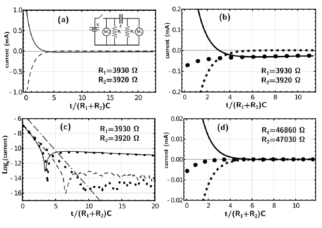
Figure 1: Current through $R_{1}$ (solid) and $R_{2}$ (dashed) from the circuit in the inset of (a) using a $505$ pF vacuum capacitor with $V=9.4$ is shown in frames (a), (b), and (c). The solid circles in (b) and (d) represent the difference between the currents into and out of the capacitor. The solid circles in (c) represent data for replacing the vacuum capacitor with a $509$ pF ceramic capacitor. All traces are raw data for a single decay. Dips that do not reach the noise baseline (around $\log_{e}|I_{R}|\approx-15$) are data acquisition artifacts.

Figs. 1 (a), (b), and (c) illustrate the decay current $I_{R_{1}}$ through $R_{1}=3930\Omega$ (solid line) and $I_{R_{2}}$ through $R_{2}=3920\Omega$ (dashed line), for the circuit shown in the inset. The vacuum capacitor has $C=505$ pF while $V=9.4$. $M_{1}$ and $M_{2}$ represent the meters that measure the voltages and by Ohm’s law these currents. A mechanical switch disconnects the battery from the RC circuit (with an open switch capacitance of less than $0.1$ pF).

Fig. 1(b) shows an enlarged segment of fig. 1(a). The solid circles represent $I_{R_{1}}+I_{R_{2}}$, indicating that the current entering the capacitor is greater than that leaving it. Fig. 1 (c) illustrates these data on a semi-log plot of the absolute value of the current. The interpretation of such graphs is best demonstrated by comparing fig. 1 (b) with (c). The dips in the semi-log plots correspond to the zero currents in fig. 1(a). After going negative (reversing direction) the current then slowly approaches zero, indicated by a downward slope in the semi-log plot. The straight dot-two-dash line in fig. 1(b) shows the results for the exponential decay with a time constant of $(R_{1}+R_{2})C$. This line is offset along the ordinate for clarity.

In addition to illustrating the vacuum capacitor decay data, the solid circles in frame (c) show the decay data from a $509$ pF ceramic capacitor for the same values of $R_{1}$ and $R_{2}$. These currents from the ceramic capacitor through each resistor are easily separated by the context in which they appear in the figure. This decay behavior appears to be a universal characteristics of capacitors.

The unequal currents into and out of a capacitor result in a net charge on the capacitor. In analogy with the net charge on a hairpin wire this charge plays a role in the decay behavior.

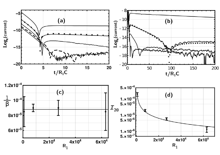
Figure 2: Decay data for the circuit in fig. 1 with $R_{2}=0$, $C=505$ pF, $V=9.4$, and increasing values of $R_{1}$ from top to bottom ($R_{1}=861,~{}7850,~{}27000,~{}63000,$ and $91600~{}\Omega$) plotted vs time constant units in frames (a) and in (b) without the $91600~{}\Omega$ data. The data for $R_{1}=63000~{}\Omega$ in frame (a) is represented by a dashed line. Model results for the $R_{1}=7850~{}\Omega$ decay are represented by solid squares. Frame (c) shows the inverse of the model’s second decay constant (the second time constant) in seconds as a function of $R_{1}$. Frame (d) presents the value of $I_{20}$ as determined from the sum of exponentials model of the data in frames (a) and (b) while the solid line represents the function $0.13/R_{1}$.

Fig. 2 presents decay data for the circuit of fig. 1(a) with the same vacuum capacitor but with $R_{2}=0$ while $R_{1}=861,~{}7850,~{}27000,~{}63000,$ and $91600~{}\Omega$. These are shown with the smallest to largest resistor values from top to bottom at $t/R_{1}C=0$ in fig. 2(a). The same order is shown in fig. 2(b) without the $R_{1}=91600~{}\Omega$ data. Each trace is an average over four decays. A moving average over $20$ data points ($2000$ data points per trace) in frame (b) has been applied to the tails of the data to mitigate overlap of the traces.

Prominent characteristics of the fig. 2 data are: (I) The first relaxation time always matches $1/R_{1}C$ within error while the second, $\beta$ (shown in fig. 2(c)), and third, $\gamma=0.0032\pm.002+(3\pm 4)\times 10^{-8}R_{1}s^{-1}$, are essentially independent of $R_{1}$. (II) Two current reversals occur for each trace (the second dip for the upper trace is not shown since it occurs at $t/\textrm{R}_{1}\textrm{C}=930$). (III) A fit of the time at which the first current reversal occurs yields $T_{1}=1.7\times 10^{-9}R_{1}+2.6\times 10^{-14}R_{1}^{2}$, while that of $T_{2}=0.00040\pm 2\times 10^{-5}s$ is independent of $R_{1}$.

III Phenomenological Model

A model for the $R_{1}=7850~{}\Omega$ data, shown as solid squares in fig. 2 (a) and (b), is given by $I=I_{10}\exp[-\alpha t]-I_{20}\exp[-\beta t]+I_{30}\exp[-\gamma t]]$. This is referred to as the sum of exponentials model. For all of the fits presented here $\alpha=1/\textrm{RC}$, where the values of R and C are determined from measurements of the individual circuit components. Errors in these measurements do not lead to noticeable differences in the model fits shown in the figures.

The parameters of this model for the $R_{1}=7850~{}\Omega$ data are $\alpha=2.27\times 10^{5},\beta=1.2\times 10^{4},\gamma=330$ and $I_{10}=10^{-3},I_{20}=2.5\times 10^{-5},I_{30}=2.8\times 10^{-7}$. This model applied to all the data in fig. 2(a) and (b) results in similar fits to that of the $R_{1}=7850~{}\Omega$ data. The two variable parameters in these fits are $I_{20}$ and $\beta$, a summary of which for the data in fig. 2 is found in (c) and (d).

To measure the decay as the charge distributes over an isolated conductor the single capacitor in fig. 2 is replaced with two in series, as shown in the inset of fig 3 (a) with switches that operate synchronously (within a millisecond while the time constant is $60$ milliseconds). When the switches are closed the isolated right plates of polypropylene capacitors $C_{1}=2.012\mu F$ and $C_{2}=2.014\mu F$ have charge and no charge, respectively. When the switches open the right plates then have a initial net charge which is distributed between them during the decay. Without a switch across $C_{2}$ the net charge on the right plates of $C_{1}$ and $C_{2}$ is initially zero (they are grounded before data collection commences). The response of the circuit for these two cases is shown in figs. 3 (b) and (c). The latter demonstrates enhancement in the non-exponential decay due to this net charge on the right plates of $C_{1}$ and $C_{2}$.

The sum of exponentials model for the voltage across $C_{2}$, shown in fig. 3, is $V_{M_{2}}=V^{in}_{f}(1-\exp[-\alpha t])+V^{out}_{f}(1-\exp[-\beta t])$ with $V^{in}_{f}$ negative. The data is presented in fig. 3 as $|V_{M_{2}}-V_{f}|$ in semilog plots where $V_{f}=V^{in}_{f}+V^{out}_{f}$ is approximated by the voltage at $t=100\mathrm{RC}$.

Figure 3: Frames (a), (c), and (d) show meter $M_{2}$ voltage data for the circuit in the inset of frame (a). Voltage data for meter $M_{1}$ is shown in frame (b). The insets in frames (b) and (c) show $C_{dyn}$ for the respective models of the $M_{2}$ data (in microfarads for (b)) while (d) shows the response for different initial voltages. The capacitors are each $2.01\mu F$. For frame (a) through (c) $R=59.5K\Omega$ with $V=9.8$. For frame (d) $R=578K\Omega$ with $V=20,0.74$, and $0.088$ with a microvolt noise baseline and error bars displayed only for a few of the data points.

When the switch across $C_{2}$ is operational the data are obtained as follows. The capacitors are first grounded. Then the switches in fig. 3 (a) are closed. The switches are opened and data is recorded for a duration of $t_{f}=100\mathrm{RC}$. The dips in fig. 3 (c) occur when $V=V_{f}$ while the magnitude of the voltage across $C_{2}$ reaches a maximum value and then decreases shortly thereafter.

Data when the switch across $C_{2}$ is always open is represented in frame (b) by the solid squares while in frame (c) by the lower trace when $t>15~{}\mathrm{RC}$. Data when this switch is operational is given by the solid lines in frame (b), the upper trace in frame (c) when $t>15~{}\mathrm{RC}$, and by all traces in frame (d). Time is expressed in time constant units, $t/\mathrm{RC}$, where $C$ is the effective capacitance of $C_{1}$ and $C_{2}$ in series. The diagonal dashed line represents exponential decay with time constant $\mathrm{RC}$. It is offset along the ordinate for clarity.

The open pentagons and filled squares are sum of exponential model predictions. For fig. 3 (b) $V=V_{10}\exp[-\alpha t]+V_{20}\exp[-\beta t]$ where $\alpha=16.7$, $\beta=0.7$, $V_{10}=10.0$, and $V_{20}=6.0\times 10^{-4}$. The tail of the data in fig. 3 (c) (causing its deviation from an exponential) is ubiquitous in RC circuits. Swantek et al. (2021) Note that this tail begins when $dV/dt$ in frame (c) changes sign.

The model predictions for the lower trace in fig. 3 (c), shown as the open hexagons, are given by $V=V_{10}\exp[-\alpha t]-V_{20}\exp[-\beta t]$ where $\alpha=16.7$, $\beta=0.5$, $V_{10}=7.0$, and $V_{20}=6.0\times 10^{-4}$. The model for the upper trace data in fig. 3 (c) with the switch operational, shown as the open hexagons, is given by $V=V_{10}\exp[-\alpha t]-V_{20}\exp[-\beta t]$ where $\alpha=16.7$, $\beta=0.2$, $V_{10}=7.0$ and $V_{20}=5.0\times 10^{-3}$.

IV Dynamic Capacitance Model

A useful parameter in modeling such behavior is the dynamic capacitance, $C_{dyn}=dQ/dV$. This can be rewritten as $C_{dyn}dV/dt=-V/R$ where $V$ is the voltage across the capacitor and $dQ$ the change in charge on the plate where $V$ is measured. Note that Kirchhoff’s law for this RC circuit is obtained from this relationship by the substitution $C_{dyn}\rightarrow C$ (for exponential decay $C_{dyn}=C$). The insets of fig. 3 (c) and (d) show the dynamic capacitances, determined from the respective sum of exponentials models, that match the data when the switch across $C_{2}$ is operational (this first order ODE then has a solution that is a sum of exponentials). At the instant when $dV/dt=0$ in frame (c) the value for $C_{dyn}$ is undefined.

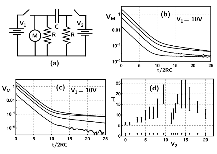
Figure 4: The decay measured for $V_{1}=10$ with different initial voltages on the right side of the polypropylene capacitor for the circuit in frame (a) with $R=274$K$\Omega$ and $C=2.01\mu$F. The switches are closed to energize the capacitor. They then open simultaneously for the discharge. Frames (b) and (c) illustrate decays for $V_{2}=0,6,9,9.8$ and $V_{2}=20,14,11.5,10.15$ from top to bottom, respectively. The time constants in seconds for the $V_{20}\exp[-\beta t]$ (plotted with error bars) and $V_{10}\exp[-\alpha t]$ (plotted with filled circles) decays are shown in frame (d).

V Surface Charge Model

Another modeling approach is to separate the amount of charge on a capacitor plate into two parts: one associated with the energy stored in between the capacitor plates, $Q^{in}$, whose electric field is confined in between the plates, and $Q^{out}$, the charge on the circuit wire and capacitor plate that facilitates the flow of current in the circuit with its electric field not confined. The superposition principle yields a response that is a sum of responses for each type of charge in this separate charge model. Let the $V_{10}\exp[-\alpha t]$ term in the above sum of exponentials model be associated with $Q^{in}$. Let $Q^{out}_{0}$ be the charge required to direct the current from the battery into $R$ before the switch is opened. This is expressed as $Q^{out}_{0}=V^{out}_{0}\tau_{out}/R$, where $\tau_{out}$ is a constant and $V^{out}_{0}$ is the voltage at the plate generated by $Q^{out}_{0}$. For smaller $R$ larger $Q^{out}_{0}$ is required to direct this larger current away from the capacitor plate and into the resistor (similar to the effect that charge on the hairpin wire has on the current flowing through the wire).

After the switch opens $V^{out}=RdQ^{out}/dt$. The loss of $Q^{out}$ is then determined from $dQ^{out}/dt=-Q^{out}/\tau_{out}$ leading to exponential decay with a time constant independent of $R$ and matching the data in fig. 2 (c). The parameters in the model term $V_{20}\exp[-\beta t]$ are $V_{20}=V^{out}_{0}$ and $\beta=1/\tau_{out}$.

The current due to this second term in the sum of exponentials model for the data in fig. 2 is $dQ^{out}/dt=Q^{out}_{0}\exp[-t/\tau_{out}]/\tau_{out}=V^{out}_{0}\exp[-t/\tau_{out}]/R_{1}$. Fig. 2(d) illustrates this with $V_{20}=V^{out}_{0}/R_{1}=.13/R_{1}$.

For the data in fig. 1 each capacitor plate has a different $Q^{out}$ value and therefore a different $V_{20}$ and $\beta$ value to account for the different decays observed from each plate. However, the $V_{10}\exp[-\alpha t]$ term is the same for both plates (with time constant $(R_{1}+R_{2})C$).

Consider the separate charge model applied to the data in fig. 3 (d). For decreasing $V$ the initial charge on the right plate of $C_{1}$ decreases. After the switches open this charge flows to the right plate of $C_{2}$, its current limited by $R$. The dip in the response of the upper trace (at $t/\mathrm{RC}=15$) transitions to a response without a dip in the middle trace (at $t/\mathrm{RC}=15$) through essentially a single exponential decay response in the lower trace at ($t/\mathrm{RC}=15$). The voltage across $C_{2}$ is measured to constantly change during the $t=0\rightarrow t_{f}$ time interval for the upper and middle traces; decreasing to minimum value then increasing toward $V_{f}$ for the upper trace and constantly decreasing toward $V_{f}$ for the middle trace. However, the voltage of the lower trace decreases until $t\approx 15\mathrm{RC}$ and then remains at this value.

This lower trace corresponds to $Q^{out}_{f}\approx 0$. Larger and smaller $Q^{out}_{f}$ result in positive and negative values of $V_{20}$ with dip and no dip responses as shown in the upper and middle traces. This is supported by fits of this data to the sum of exponential model with parameters $V_{20}/V_{10}=-8.0\times 10^{-5},-4.3\times 10^{-7}$, and $6.6\times 10^{-4}$ for the upper, lower and middle traces, respectively. With judicious choice of $R$ and $V$ it is therefore possible to generate only the $V=V_{10}\exp[-\alpha t]$ exponential decay across $C_{2}$.

The $\alpha$ decay constant in the first term of the sum of exponentials model is unaffected by such variations in the initial voltage in $V$ while $\beta$ varies. This is evidence for the model that separates charges into $Q^{in}$ and $Q^{out}$. Although not shown in this figure, $V_{M_{1}}$, for the different initial voltages shown in fig. 3(d), varies in essentially the same manner as that shown in fig. 3(b), indicating different values of $Q^{out}$ for left and right plates of $C_{1}$.

Different values of $Q^{out}_{0}$ on each capacitor plate are also generated by applying different initial voltages to each plate using the fig. 4 (a) circuit. Fixing the initial voltage on the left plate while varying the initial voltage on the right plate results in variation of $\tau=1/\beta$ but not the time constant $2\mathrm{RC}=1/\alpha$ associated with $Q^{in}$ in the sum of exponentials model (which is additional evidence for the separation of charges model). Although not shown, the magnitude of $V_{20}/V_{10}$ for these data vary in a similar manner to $\tau=1/\beta$ in fig. 4(d) ranging in value from $1.2\times 10^{-4}$ to $2.5\times 10^{-4}$. Evidence that inductance has no impact on these results is given in fig. 3(d) and fig. 4 where only a variation of the initial voltage generates a variety of sum of exponentials behavior while the circuit geometry (and therefore the inductance) remains the same.

The geometry of a circuit increases the difficulty in calculating $Q^{out}$ from Maxwell’s equations. Muller (2012) Yet the data illustrate similar but simple (a sum of exponentials) behavior for dissimilar capacitors. An example is the small ceramic and much larger vacuum capacitor both with the same capacitance but with dissimilar areas generated by the circuit wires and areas of the capacitor plates. In addition, currents due to $Q^{out}$ are measured even after $Q^{in}$ has exponentially decayed over a hundred $\mathrm{RC}$ time constants. During such times $Q^{in}$ is so small that it cannot effect the currents due to $Q^{out}$ that are observed. Another decoupling of $Q^{out}$ occurs between it and the third term in the sum of exponentials model for even longer times, as shown for the $R_{1}=861\Omega$ and $R_{1}=7850\Omega$ decays in fig. 2. This indicates that the third decay is a mode of relaxation different from that of the second decay.

VI Discussion

Constructing a numerical model that predicts only a single exponential decay for an RC circuit from Maxwell’s equations is nontrivial. Preyer (2002) Yet, the data indicating sequential decays with divergent time constants is supported by the simple sum of exponentials model.

A full understanding requires more effort in modeling and data collection. For example, one might conjecture that $Q^{out}$ influences the response of inductors. The effect of such charges in circuits with energy relaxation determined by radiative rather than thermal mechanisms is also of interest, an example being a superconducting LC circuit. The loss due to conversion of the electrical energy stored in the capacitor into mechanical energy (or into more complicated circuit components) may, in addition, be influenced by $Q^{out}$.

The simplicity of the Kirchhoff exponential decay model and its ability to match well the initial decay data are factors that have allowed the results presented above to have been overlooked. Another reason is that the deviations from exponential decay, documented above, are small. An additional reason involves the ubiquitous use of dielectric capacitors. The novel behavior described above might then be attributed to complicated relaxation mechanisms in the dielectric rather than to a fundamental characteristic of a capacitor. A revision of circuit models to account for such behavior is therefore needed, particularly in applications that use a capacitor as a sensor and those that require precision data, such as is found in dielectric spectroscopy and quantum measurements.

VII Conclusions

The decay of the electrical energy in a resistor-vacuum capacitor circuit involves multiple sequential relaxation processes, with increasing time constants, separated by transition regions that involve a change in current direction. This novel behavior differs fundamentally from the single exponential decay predicted by circuit simulation software when applied to a vacuum capacitor-resistor circuit. A microscopic understanding of the sum of exponentials model involves charge on the surface of the circuit components.

Appendix 1: Methodology

Two oscilloscopes (Picoscope models $4262$ and $4226$) with either $16$ bit resolution at $10$ MS/s or $12$ bit resolution at $50$ MS/s along with a digital voltmeter (Keysight 34465A with input impedance greater than $1~{}\textrm{G}\Omega$) were used to collect data. The oscilloscope probes were set on a x$10$ scale with an input resistance $10~{}\textrm{M}\Omega$ and a capacitance of $15$ pF. A Comet vacuum capacitor model CFMN-500AAC/12-DE-G was used in figs. 1, 2 (inductance $<6~{}\textrm{nH}$).

A mechanical switch coupled and decoupled the battery from the circuit. No difference in the measurements was observed between the use of toggle or micro switches. The circuit layout was similar to that shown in fig. 1. The wire diameter was $0.5$ mm. All the circuits used $1/4$ W $1\%$ metal film resistors (inductance $<2~{}\textrm{nH}$).

The disk ceramic capacitor (diameter $3\times 10^{-3}~{}\textrm{m}^{2}$ and thickness $2\times 10^{-3}~{}\textrm{m}$) allowed the area enclosed by the circuit to vary from $3\times 10^{-4}$ to $3\times 10^{-2}$ $\textrm{m}^{2}$. However, the data shown in fig. 1 (b) did not then change noticeably, demonstrating that inductance is not an important parameter in these results. The similarity in response of a circuit where $dI/dt$ varies by five orders of magnitude is additional evidence against inductance being a important variable.

Appendix 2: Frequency Domain Data

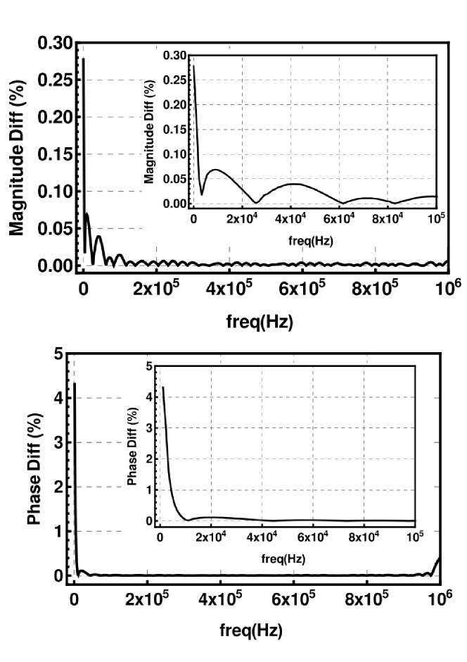
Figure 5: Percent difference of the current between the data and exponential decay for the circuit used in fig. 2b. The upper and lower frames are magnitude and phase graphs.

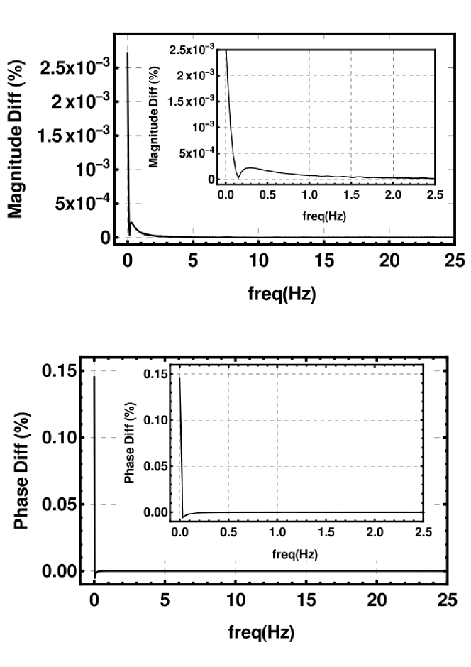
Figure 6: Frequency domain results for the circuit used in figs. 3b presented in the same manner as that in fig. 5.

The above circuit behavior can also be expressed in the frequency domain. However, the decays with longer time constants predominately manifest at the low end of the spectrum. Since the exponential decay spectrum is largest at these low frequencies it is difficult to resolve on a Bode plot the small differences between the decays with longer time constants and that of the single exponential decay determined by the R and C values. On the other hand, in the time domain the decays with longer time constants occur on a zero background since the initial exponential decay has essentially vanished.

To better illustrate the real and ideal behavior in the frequency domain the difference between the currents in the real and ideal circuits is first determined as a function of frequency. This difference when divided by the ideal current at each frequency yields a percent difference. The magnitude and phase of these percent differences are presented in fig. 5 for the circuit used in fig.2 with $R_{1}=7850~{}\Omega$ and $C=505$ pF. Results from this same procedure for the $R_{1}=59.5~{}\mathrm{K}\Omega$ and $C=1~{}\mu$F circuit used to collect the data shown in fig. 3b are given in fig. 6 .

References

- Scott (1975) Alwyn C. Scott, “The electrophysics of a nerve fiber,” Rev. Mod. Phys. 47, 487–533 (1975).
- Didier and Fazio (2012) N. Didier and R. Fazio, “Putting mechanics into circuit quantum electrodynamics,” Comptes Rendus Physique 13, 470–479 (2012).
- Teufel et al. (2011) J Teufel, Dale Li, M Allman, K Cicak, Adam Sirois, J Whittaker, and R Simmonds, “Circuit cavity electromechanics in the strong-coupling regime,” Nature 471, 204–8 (2011).
- Córcoles et al. (2011) A. Córcoles, J. Rozen, M. Rothwell, G. Keefe, D. Vincenzo, M. Ketchen, J. Chow, C. Rigetti, J. Rohrs, M. Borstelmann, and M. Steffen, “Energy relaxation mechanisms in capacitively shunted flux qubits,” Bulletin of the American Physical Society (2011).
- Gustavsson et al. (2016) S. Gustavsson, F. Yan, G. Catelani, J. Bylander, A. Kamal, J. Birenbaum, D. Hover, D. Rosenberg, G. Samach, A. Sears, S. Weber, J. Yoder, J. Clarke, A. Kerman, F. Yoshihara, Y. Nakamura, T. Orlando, and W. Oliver, “Suppressing relaxation in superconducting qubits by quasiparticle pumping,” Science 354 (2016), 10.1126/science.aah5844.
- Kohlrausch (2009) R. Kohlrausch, “Theorie des elektrischen rückstandes in der leidener flasche,” Ann. Phys. 167, 56–58 (2009).
- Kramer (2012) F. Kramer, Broadband Dielectric Spectroscopy (Springer Berlin Heidelberg, 2012) pp. 48–51.
- Jonscher (1999) A. K. Jonscher, “Dielectric relaxation in solids,” Journal of Physics D: Applied Physics 32, R57–R70 (1999).
- Feldman et al. (2005) Y. Feldman, A. Puzenko, and Y. Ryabov, “Dielectric relaxation phenomena in complex materials,” Advances in Chemical Physics 133, 1 – 125 (2005).
- Westerlund and Ekstam (1994) S. Westerlund and L. Ekstam, “Capacitor theory,” IEEE Transactions on Dielectrics and Electrical Insulation 1, 826–839 (1994).
- Allagui et al. (2022) Anis Allagui, Di Zhang, and Ahmed Elwakil, “Further Experimental Evidence of the Dead Matter Has Memory Conjecture in Capacitive Devices,” arXiv e-prints , arXiv:2206.15043 (2022), arXiv:2206.15043 [physics.app-ph] .
- Ortigueira et al. (2023) Manuel Ortigueira, Valeriy Martynyuk, Volodymyr Kosenkov, and Arnaldo Batista, “A new look at the capacitor theory,” Fractal and Fractional 7 (2023), 10.3390/fractalfract7010086.
- solutions (2019) Cadence PCB solutions, “Capacitor self-resonant frequency and signal integrity,” (2019).
- Muller (2012) R. Muller, “A semiquantitative treatment of surface charges in dc circuits,” American Journal of Physics 80, 782–788 (2012), https://doi.org/10.1119/1.4731722 .
- Sommerfeld (1952) A. Sommerfeld, in Electrodynamics (Academic, New York, 1952) pp. 125–130.
- Heald (1984) M. A. Heald, “Electric fields and charges in elementary circuits,” American Journal of Physics 52, 522–526 (1984), https://doi.org/10.1119/1.13611 .
- Chabay and Sherwood (2019) R. Chabay and B. Sherwood, “Polarization in electrostatics and circuits: Computing and visualizing surface charge distributions,” American Journal of Physics 87, 341–349 (2019), https://doi.org/10.1119/1.5095939 .
- Schade et al. (2019) Nicholas Schade, David Schuster, and Sidney Nagel, “A nonlinear, geometric hall effect without magnetic field,” Proceedings of the National Academy of Sciences 116, 201916406 (2019).
- Preyer (2002) N. W. Preyer, “Transient behavior of simple rc circuits,” American Journal of Physics 70, 1187–1193 (2002), https://doi.org/10.1119/1.1508444 .
- Griffiths (1989) D. J. Griffiths, (Introduction to Electrodynamics: second edition). (Prentice-Hall, 1989) pp. 277–278.
- Moreau (1989) W R Moreau, “Charge distributions on dc circuits and kirchhoff’s laws,” European Journal of Physics 10, 286 (1989).
- Klee (2020) M. M. Klee, “Surface charges from a sensing pixel perspective,” American Journal of Physics 88, 649–660 (2020), https://doi.org/10.1119/10.0001435 .
- Swantek et al. (2021) J. L. Swantek, T. D’Esposito, J. Brannum, and F. V. Kowalski, “Dielectric relaxation affected by a monotonically decreasing driving force: An energy perspective,” Journal of Applied Physics 130, 154101 (2021).