Enhancing gravitational wave anisotropies with peaked scalar sources

Abstract

Gravitational wave (GW) backgrounds of cosmological origin are expected to be nearly isotropic, with small anisotropies resembling those of the cosmic microwave background. We analyse the case of a scalar-induced GW background and clarify in the process the relation between two different approaches to calculating GW anisotropies. We focus on GW scenarios sourced by a significantly peaked scalar spectrum, which are frequently considered in the context of primordial black holes production. We show that the resulting GW anisotropies are characterised by a distinct frequency dependence. We explore the observational consequences concentrating on a GW background enhanced in the frequency band of space-based GW detectors. We study the detectability of the signal through both cross-correlations among different space-based GW detectors, and among GW and CMB experiments.

1 Introduction

The detection of a stochastic gravitational wave background (SGWB) is one of the key targets of gravitational wave astronomy. Given the increasing sensitivity of ground based detectors [1, 2], and the tantalising hints of a signal at NANOGrav [3], the detection of a background of astrophysical origin is eagerly anticipated. In addition to the astrophysical background [4], one should also expect the existence of a cosmological GW background (CGWB). Since the universe is, to a good approximation, transparent to gravitational waves below the Planck scale, the CGWB provides an excellent handle on the physics of the primordial universe (see for example the reviews in [5, 6]).
The CGWB may arise from a variety of processes in the early universe, from inflation to later sources including (p)re-heating dynamics, phase transitions, cosmic strings, and primordial black holes (PBH) (see [5] for a review). Remarkably, the GW signal associated to several such sources may be detected in the near future. Indeed, the corresponding frequencies are the one accessed by ground-based interferometers such as ET [7], CE [8] $(1\text{--}10^{3}\,\rm Hz)$ and space-based experiments including LISA [9], Taiji [10] $(10^{-4}\text{--}10^{-1}\,\rm Hz)$, all of which are expected to become operational by 2035.
The GW background generated during inflation stands out in that (i) it is universal in nature and (ii) it may span a wide range of frequencies, from the CMB up to (and above) laser interferometer scales. In single-field slow-roll scenarios, the amplitude of this background is directly related to the energy scale at which inflation occurs. Efforts to detect this background using the B-mode polarisation of the CMB have so far led to increasingly stringent constraints on the tensor-to-scalar ratio [15, 16, 17], the most recent one being $r<0.032$ [18]. As a result of the ever-improving experimental bounds, various inflationary models have fallen by the wayside. Future CMB experiments like CMB-S4 [19], Simons Observatory [20] and LiteBIRD [21] will be able to probe this background for values of the tensor-to-scalar ratio down to $r\sim 10^{-3}$ allowing us to further rule in(out) several classes of inflationary models.

The CMB-S4/LiteBIRD threshold on $r$ is particularly significant in that it will put to the test celebrated models of inflation such as the Starobinsky model [22] and (in the large field limit [23]) Higgs inflation. We stress therefore that, although direct detection of a SGWB from single-field slow-roll models is beyond the reach of most PTAs and interferometers (with the possible exception of the proposed BBO [24] in the deciHz range), the lack of detection itself will be almost equally as informative. Crucially, GW detection by upcoming experiments would point to a number of interesting inflationary scenarios, including multi-field models (see e.g. [25, 26, 27, 28, 29, 30, 31, 32, 33, 34, 35]), theories featuring alternative symmetry breaking patterns [36, 37, 38, 39, 40], and non-attractor phases [41, 42] (see [6] for a comprehensive review).
A SGWB detection will also provide the opportunity to test its dependence on direction. Most cosmological sources of GWs are known to be predominantly isotropic, with a small level of anisotropy that may arise from i) the specific production mechanism and ii) propagation in a perturbed universe. While the former anisotropies are typically model-dependent the latter are fairly universal in nature, being a consequence of the fact that the universe is not perfectly homogeneous and isotropic [48, 49, 50, 51, 52]. The anisotropies of the CGWB may therefore hold precious information on the early universe. Understanding their behaviour is also a critical step towards being able to tell them apart from anisotropies of astrophysical origin [63, 64, 65, 66, 67, 68, 69, 70, 71, 72, 73], which act as a foreground for the CGWB.
Propagation anisotropies [48] are similar in origin to those of the CMB and have been studied via a Boltzmann approach in [49, 50, 51]. We will point out how the two approaches (in [48] and [49, 50, 51] respectively) are related to each other under certain assumptions about the behaviour of the primordial perturbations as well as the time when GW are generated.
An important, ever-present, source of cosmological GW is the background sourced at second order in the primordial curvature perturbations [74, 75, 76, 77]. At linear order in perturbation theory tensor and scalar modes are decoupled from each other. However, this is no longer the case at second order: as the primordial scalar perturbations re-enter the horizon, they source GW via their second order anisotropic stress. Whenever these scalar perturbations have spectra peaked at scales which re-enter the horizon during the radiation domination epoch, the resulting scalar induced gravitational waves (SIGW) may have an amplitude large enough to be detected at interferometer scales. For sufficiently peaked spectra, possible in inflationary models with significant primordial black hole (PBH) production (see e.g. [78] for a review), this small-scale enhancement imparts a distinct spectral shape to the SIGW and its anisotropies. We will show how this also leads to a significant enhancement in the anisotropy spectrum at certain frequencies, with potentially observable consequences. The frequency dependence of the anisotropies is present not just for the SIGW, but also for any other SGWB whose spectral shape deviates from a power law (e.g. (p)reheating, phase transitions, cosmic strings [5]). See also [79] for a general review.

This paper is organised as follows. In Sec. 2 we first review the Boltzmann approach to the SGWB anisotropies and discuss the role of the GW initial conditions. We then demonstrate how and under what assumptions the result of [48] can be related to those of the Boltzmann approach. In Sec. 3 we discuss the frequency dependence of the anisotropy spectrum for the SIGW. We show that if the primordial scalar power spectrum is sharply peaked at certain scales, the resulting SIGW anisotropies can be enhanced at certain frequencies by a factor $\mathcal{O}(10\text{--}100)$ relative to the anisotropies for a standard power-law spectrum. We then discuss the implications of this enhancement for the detection of GW anisotropies using LISA-Taiji and BBO. Finally, we present our conclusions in Sec. 4.

2 Anisotropies of SGWB

In this section we start by reviewing the propagation anisotropies of the SGWB, both via the Boltzmann approach of refs. [49, 50, 51] and via the calculation in [48]. As discussed in ref. [49], the Boltzmann formalism relies on the geometrical optics approach to GW propagation which is valid for GW whose wavelengths are much smaller than the length scales over which the background curvature varies [80, 81]. The same holds for the approach of [48]. Later in this section we discuss the relation between these results and the role of the GW initial conditions. The results we develop here will be applied in Sec. 3 to study GW anisotropies from scalar induced gravitational waves.

2.1 Boltzmann approach to SGWB anisotropies

We begin with a brief review of the main results of [49, 50, 51]. The starting point is the distribution function for gravitons $f(x^{\mu},p^{\mu})$. Here $x^{\mu},p^{\mu}$ denote the position and momentum of the gravitons with $p^{\mu}=dx^{\mu}/d\lambda$, $\lambda$ being the affine parameter along the graviton trajectory which, in the geometric optics limit, is given by the null geodesics of the perturbed spacetime. The evolution of the distribution function is governed by the Liouville equation

$$\frac{df}{d\lambda}=C[f(\lambda)]+I[f(\lambda)],$$ (2.1)

where $C$ and $I$ are the collision and injection terms. The collision term is generally absent since gravitons are decoupled below the Planck scale. For stochastic backgrounds of cosmological origin, the injection term can be treated as an initial condition of the distribution [50, 51]. Thus, one must solve the free Boltzmann equation $df/d\lambda=0$ in the perturbed universe. One can write it as

$$\frac{df}{d\eta}=\frac{\partial f}{\partial\eta}+\frac{\partial f}{\partial x^{i}}\frac{dx^{i}}{d\eta}+\frac{\partial f}{\partial q}\frac{dq}{d\eta}=0.$$ (2.2)

Here,

$$q\,\equiv\,|\vec{p}|a$$ (2.3)

is the comoving momentum of the gravitons, $a$ is the cosmological scale factor, and $\hat{n}=\hat{p}$ is the direction of propagation. In the Newtonian gauge with $\Phi$ and $\Psi$ as the large-scale scalar potentials we have,

$$ds^{2}=a^{2}(\eta)\left[-(1+2\Phi)d\eta^{2}+(1-2\Psi)\delta_{ij}dx^{i}dx^{j}\right],$$ (2.4)

and the Boltzmann equation at first order in $\Phi,\Psi$ can be written as [50, 51],

$$\frac{\partial f}{\partial\eta}+\frac{\partial f}{\partial x^{i}}n^{i}+q\frac{\partial f}{\partial q}\left[\frac{\partial\Psi}{\partial\eta}-\frac{\partial\Phi}{\partial x^{i}}n^{i}\right]=0.$$ (2.5)

The total SGWB energy density observed today is given by

$$\rho_{\rm GW}(\eta_{0},\vec{x}_{0})=\int d^{3}p\,pf(\eta_{0},\vec{x_{0}},q,\hat{n})\,,$$ (2.6)

and the more commonly used fractional density parameter $\Omega_{\rm GW}(q)$ is defined as [82]

$$\rho_{\rm GW}(\eta_{0},\vec{x}_{0})=\rho_{cr}\int d\ln q\,\Omega_{\rm GW}(\eta_{0},\vec{x}_{0},q),$$ (2.7)

where $\rho_{cr}$ is the critical energy density of the universe. Upon expanding the distribution function into a homogeneous and isotropic part $\bar{f}(q)$ and a perturbation $\delta f=-q\Gamma(\eta,\vec{x},q,\hat{n})\partial{\bar{f}}/\partial{q}$ one obtains the following (very reminiscent of the analogous one in the CMB context) equation [50, 51],

$$\Gamma(\eta_{0},\vec{x}_{0},\hat{n},q)=\underbrace{\Gamma(\eta_{\rm i},\vec{x}_{i},q)}_{\Gamma_{I}}+\underbrace{\Phi(\eta_{\rm i},\vec{x}_{i})+\int_{\eta_{\rm i}}^{\eta_{0}}d\eta(\Phi^{\prime}+\Psi^{\prime})}_{\Gamma_{S}},$$ (2.8)

where $\eta_{0},\vec{x}_{0}$ correspond to the time and position of observation and one has $\vec{x}_{i}=\vec{x}_{0}-(\eta_{0}-\eta_{i})\hat{n}$. The first term on the right-hand side (R.H.S). denotes the initial perturbation at the time of emission $\eta_{i}$ while the second and third terms arise due to propagation in an inhomogeneous universe, analogous to the Sachs-Wolfe (SW) and integrated Sachs-Wolfe (ISW) effects for the CMB. As pointed out in [51], for adiabatic initial conditions the term $\Gamma_{I}$ is also correlated with the scalar term and contributes to the SW effect for gravitons. We explicitly evaluate this term in Sec. 2.1.1 for the case of single clock inflation.

The GW anisotropy observed today is defined as [51, 50],

$$\delta_{\rm GW}(\eta_{0},\vec{x}_{0},\hat{n},q)\equiv\frac{\omega_{\rm GW}(\eta_{0},\vec{x}_{0},\hat{n},q)}{\overline{\Omega}_{\rm GW}(\eta_{0},q)}-1=\left[4-\frac{\partial\ln\overline{\Omega}_{\rm GW}(\eta_{0},q)}{\partial\ln q}\right]\Gamma(\eta_{0},\vec{x}_{0},\hat{n},q),$$ (2.9)

where the quantity $\omega_{\rm GW}$ is given by

$$\Omega_{\rm GW}(\eta,\vec{x},q)=\frac{1}{4\pi}\int d^{2}\hat{n}\,\omega_{\rm GW}(\eta,\vec{x},q,\hat{n}),$$ (2.10)

with $\overline{\Omega}_{\rm GW}$ denoting the spatial average of $\Omega_{\rm GW}(q,\vec{x})$. In terms of the distribution function we have [51, 50],

$$\overline{\Omega}_{\rm GW}(q,\eta)=\frac{4\pi}{\rho_{\rm cr}}\left(\frac{q}{a}\right)^{4}\,\bar{f}(q).$$ (2.11)

We can now calculate how the initial condition $\Gamma_{I}$ is related to the initial density fluctuation $\delta\rho_{\rm GW}$, with $\rho_{\rm GW}(\eta_{i},\mathbf{x})\equiv\bar{\rho}_{\rm GW}(\eta_{i})+\delta\rho_{\rm GW}(\eta_{i},\mathbf{x})$. This will then be used in Sec. 2.1.1 to obtain $\Gamma_{I}$ in terms of the primordial potential $\Phi$. One finds:

$$\rho_{\rm GW}(\eta_{i},\vec{x}) =\int d^{3}p\,p\bar{f}(q)\left[1-\frac{\partial\ln\bar{f}}{\partial\ln q}\Gamma(\eta_{i},\vec{x},q,\hat{n})\right]$$

$$=\frac{4\pi}{a^{4}}\int dq\,\bar{f}(q)q^{3}-\frac{1}{a^{4}}\int dq\frac{\partial\bar{f}}{\partial q}q^{4}\int d^{2}\hat{n}\,\Gamma_{I},\quad\text{with }\Gamma_{I}\equiv\Gamma(\eta_{i},\vec{x},q,\hat{n})\,.$$ (2.12)

If the only contribution to $\Gamma_{I}$ arises from the adiabatic primordial perturbations, which is the scenario we are interested in here, $\Gamma_{I}$ can be safely assumed to be $q$-independent. In this case, upon integrating by parts the integral over $q$ on the R.H.S., one arrives at

$$\rho_{\rm GW}(\eta_{i},\vec{x})=\frac{4\pi}{a^{4}}\int dq\,\bar{f}(q)q^{3}\left(1+4\int\frac{d^{2}\hat{n}}{4\pi}\,\Gamma_{I}\right)\equiv\bar{\rho}_{\rm GW}+\delta\rho_{\rm GW}.$$ (2.13)

From here one can see that the intrinsic density perturbation in the Newtonian gauge at the initial time $\eta_{i}$ is related to the monopole of $\Gamma_{I}$ by

$$\frac{\delta\rho_{\rm GW}}{\bar{\rho}_{\rm GW}}=4\int\frac{d^{2}\hat{n}}{4\pi}\,\Gamma_{I}\equiv 4\Gamma_{I}^{(0)}.$$ (2.14)

We are already familiar with this result from the CMB ($\Gamma=\Theta\equiv\delta T/T$), where we have $\delta\rho_{\gamma}/\bar{\rho}_{\gamma}\equiv\delta_{\gamma}=4\Theta_{0}$, $\Theta_{0}$ being the intrinsic temperature fluctuation at recombination. Note that in our analysis we will neglect any higher order multipole terms in $\Gamma_{I}$ and therefore from now on we will simply identify $\Gamma_{I}=\Gamma_{I}^{(0)}=\delta\rho_{\rm GW}/(4\bar{\rho}_{\rm GW})$.

When to evaluate initial conditions. For GW detectable at interferometer scales, the initial conditions are set early during radiation domination (RD) since that is when these GW are generated (e.g. from 1st order phase transitions, second order GW from scalar perturbations). Similarly, for inflationary GW to be tested e.g. at interferometers, RD is when the GW modes re-enter the horizon and start to propagate freely. It is only once the GW modes become sub-horizon ($q\ll\mathcal{H}$ ) that $\rho_{\rm GW}\propto a^{-4}$ and one can correspondingly think of them as behaving like relativistic particles. Instead, for superhorizon modes ($q\gg\mathcal{H}$) the energy density scales as $\rho_{\rm GW}\propto a^{-2}$ [83].

2.1.1 Initial conditions for GW anisotropies

We now calculate the initial GW overdensity $\delta\rho_{\rm GW}(\eta_{i},\mathbf{x})$ at the time of emission $\eta_{i}$, assuming that the primordial perturbations from inflation are adiabatic. These perturbations correspond to common, local time shifts in all background quantities as a result of which they have the property that for two different species $i$ and $j$,

$$\frac{\delta\rho_{i}}{(1+\mathsf{w}_{i})\bar{\rho}_{i}}=\frac{\delta\rho_{j}}{(1+\mathsf{w}_{j})\bar{\rho}_{j}}\,,$$ (2.15)

where $\mathsf{w}_{i}$ denotes the equation of state parameter for species $i$. Keeping this in mind, we can now easily relate the initial GW density perturbation to the potential $\Phi$ (we neglect any anisotropic stresses so that $\Phi=\Psi$). Firstly, note that the super-horizon solution for the photon density contrast during radiation domination is given by [84],

$$\delta_{\gamma}=-2\Phi\,.$$ (2.16)

Therefore, by adiabaticity (neglecting sub-leading slow-roll corrections) and using the fact that $\mathsf{w}_{\rm GW}=\mathsf{w}_{\gamma}=1/3$, we have,

$$\frac{\delta\rho_{\rm GW}}{\bar{\rho}_{\rm GW}}=\delta_{\gamma}=-2\Phi\ \implies\Gamma_{I}=\frac{1}{4}\frac{\delta\rho_{\rm GW}}{\bar{\rho}_{\rm GW}}=-\frac{1}{2}\Phi\,,$$ (2.17)

with all the quantities evaluated at the initial time $\eta_{i}$.

Alternatively, one can obtain the result of Eq. (2.17) for the initial density perturbation in the Newtonian gauge by first converting the metric element to an unperturbed form

$$ds^{2}=a^{2}(\tilde{\eta})\left[-d\tilde{\eta}^{2}+\delta_{ij}d\tilde{x}^{i}d\tilde{x}^{j}\right]$$ (2.18)

via the coordinate transformation $x^{\mu}\to\tilde{x}^{\mu}\equiv x^{\mu}+\xi^{\mu}$ with [85]

$$\xi^{0}=\begin{dcases}-\frac{1}{5}\zeta\eta,&\text{M.D.}\\ -\frac{1}{3}\zeta\eta,&\text{R.D.}\end{dcases}$$ (2.19)

and

$$\xi^{i} =-\zeta x^{i}\,.$$ (2.20)

In the unperturbed coordinates we have $\delta\tilde{\rho}_{\rm GW}=0$. Thus, the density perturbation $\delta\rho_{\rm GW}$ in the Newtonian gauge is,

$$\delta\rho_{\rm GW} =\delta\tilde{\rho}_{\rm GW}+\bar{\rho}_{\rm GW}^{\prime}\xi^{0}$$

$$=-4\mathcal{H}\bar{\rho}_{\rm GW}\xi^{0}\,,$$ (2.21)

where $\bar{\rho}_{\rm GW}^{\prime}=-3\mathcal{H}(1+\mathsf{w}_{\rm GW})\bar{\rho}_{\rm GW}$. During radiation domination one then finds,

$$\frac{\delta\rho_{\rm GW}}{\bar{\rho}_{\rm GW}}=-2\Phi\,,$$ (2.22)

where we used the radiation domination expression for $\xi^{0}$ given in Eq. (2.19) and the relations $a\propto\eta$, and $\Phi=-2\zeta/3$. In contrast, for the CMB the relevant epoch for the initial conditions is that of matter domination and one obtains the standard result [85]

$$\delta_{\gamma}=-4\mathcal{H}\xi^{0}=-\frac{8}{3}\Phi,$$ (2.23)

where the matter domination relations $a\propto\eta^{2}$ and $\Phi=-3\zeta/5$ have been used.

Putting together Eqs. (2.8) and (2.17), the total anisotropy observed today for GW produced during the radiation dominated epoch, under the assumption of adiabatic initial conditions, is given by

$$\Gamma(\eta_{0},\vec{x}_{0},\hat{n}) =\underbrace{\Gamma(\eta_{i},\vec{x}_{i})}_{\Gamma_{I}}+\Phi(\eta_{i},\vec{x}_{i})+\int_{\eta_{\rm i}}^{\eta_{0}}d\eta(\Phi^{\prime}+\Psi^{\prime})$$

$$=\frac{1}{2}\Phi(\eta_{i},\vec{x}_{i})+\int_{\eta_{\rm i}}^{\eta_{0}}d\eta(\Phi^{\prime}+\Psi^{\prime})$$ (2.24)

$$=-\frac{1}{3}\zeta(\eta_{i},\vec{x}_{i})+\int_{\eta_{\rm i}}^{\eta_{0}}d\eta(\Phi^{\prime}+\Psi^{\prime})\,,$$

where we remind the reader that $\vec{x}_{0}=\vec{x}_{i}+(\eta_{0}-\eta_{i})\hat{n}$. Thus, although the large scale GW anisotropies have the same origin as those of the CMB, the coefficient appearing in front of the potential $\Phi$ is $1/2$ instead of $1/3$ due to the fact that the gravitons of interest (for direct detection at intermediate and small scales) start propagating during radiation domination. Indeed, if instead recombination took place during radiation domination, then the CMB SW effect would also be modified accordingly [86].

The effect of primordial isocurvature perturbations on the GW anisotropy has also been studied recently in [54, 87]. The isocurvature perturbations modify the GW anisotropy as [54],

$$\Gamma_{\rm iso}=\Gamma_{\rm ad}+\frac{1}{3}(1-f_{\rm GW})S_{\rm GW}\,.$$ (2.25)

Here $f_{\rm GW}\equiv\rho_{\text{GW}}/\rho_{\text{tot}}$, with $\rho_{\text{tot}}$ the total energy density, and $\Gamma_{\rm ad}$ is the GW anisotropy, assuming adiabatic initial conditions, given in Eq. (2.1.1). $S_{\rm GW}$ is the GW isocurvature perturbation w.r.t photons defined as $S_{{\rm GW}}\equiv 3(\zeta_{{\rm GW}}-\zeta_{\gamma})$, with $\zeta_{i}=-\Psi-H{\delta\rho_{i}}/{\dot{\bar{\rho}}_{i}}$ the curvature perturbation on the hyper-surfaces of uniform energy of the fluid $i$.

2.2 Uniform density gauge calculation

We now compute the propagation anisotropy following ref. [48]. The starting point for the calculation of [48] is the uniform density gauge during matter domination for which the metric is given by [88],

$$ds^{2}=a^{2}(\eta)\left[-d\eta^{2}+(1+2\zeta)\delta_{ij}dx^{i}dx^{j}-\frac{4}{5aH}\partial_{i}\zeta d\eta dx^{i}\right]\,.$$ (2.26)

To facilitate the comparison with the results of the previous section, we compute here the GW anisotropy via the Boltzmann approach working in the uniform density gauge given by Eq. (2.26). Although ref. [48] proceeds in a slightly different manner, the results are equivalent. For completeness we also report the original calculation of ref. [48] as well as some details related to the Boltzmann approach in Appendix A.

To solve the Boltzmann equation (2.2), we express more conveniently its various terms. We write the graviton 4-momentum $P^{\mu}$ in terms of the magnitude of the physical momentum $p$ and the direction of propagation $\hat{n}$ as (see Appendix A for the details)

$$P^{\mu}=\frac{p}{a}\left(1-\frac{2}{5aH}\partial_{i}\zeta n^{i},(1-\zeta)\hat{n}\right)\,.$$ (2.27)

From this one can simply read the derivative

$$\frac{dx^{i}}{d\eta}=\frac{P^{i}}{P^{0}}=n^{i}\,.$$ (2.28)

Note that we only need this term at zeroth order, since it multiplies $\partial f/\partial x^{i}$ which is a first order quantity. Next, we need $dq/d\eta$. After some manipulations (see Appendix A), one finds

$$\frac{dq}{d\eta}=\frac{1}{5}q\,\partial_{i}\zeta n^{i}\,.$$ (2.29)

Using the above results, one can finally write

$$\frac{\partial f}{\partial\eta}+\frac{\partial f}{\partial x^{i}}n^{i}+\frac{1}{5}q\partial_{i}\zeta n^{i}\frac{\partial f}{\partial q}=0\,.$$ (2.30)

In terms of the zeroth order distribution $\bar{f}$ and the first order perturbation $\delta f=-q\Gamma(\eta,\vec{x},q,\hat{n})\partial{\bar{f}}/\partial{q}$ one obtains,

$$\frac{\partial\Gamma}{\partial\eta}+n^{i}\frac{\partial\Gamma}{\partial x^{i}} =\frac{1}{5}\frac{\partial\zeta}{\partial x^{i}}n^{i}\,.$$ (2.31)

This equation can be integrated along the line of sight to give,

$$\Gamma(\eta,\vec{x}_{0},q,\hat{n})=\underbrace{\Gamma(\eta_{\rm in},\vec{x}_{i},q,\hat{n})}_{\Gamma_{I}}-\underbrace{\frac{1}{5}\zeta(\eta_{\rm in},x_{i})}_{\Gamma_{S}}\,,$$ (2.32)

where $\vec{x}_{0}=\vec{x}_{i}+(\eta-\eta_{\rm in})\hat{n}$. The curvature perturbation at the observer’s position can be ignored since it does not have any direction dependence. Note that the Authors of ref. [48] consider the case of single-field inflation and assume adiabatic primordial perturbations. Since the gauge of Eq. (2.26) is the uniform matter density gauge, it must also be the uniform GW density gauge, i.e. by adiabaticity one finds

$$\frac{\delta\rho_{\rm GW}}{\bar{\rho}_{\rm GW}}=\frac{4\delta\rho_{\rm m}}{3\bar{\rho}_{\rm m}}=0\implies\Gamma_{I}=0,$$ (2.33)

where we have used Eq. (2.14). Using this result in Eq. (2.32), the relation in Eq. (2.9) between the GW anisotropy $\delta_{\rm GW}$ and $\Gamma$, and Eq. (2.11), one obtains

$$\delta_{\rm GW}(q,\eta_{0},\hat{n}) =-\frac{1}{5}\zeta(\eta_{i},\vec{x}_{i})\left[4-\frac{\partial\ln\overline{\Omega}_{\rm GW}}{\partial\ln q}\right]=\frac{1}{5}\zeta(\eta_{i},\vec{x}_{i})\frac{\partial\ln\bar{f}(q)}{\partial\ln q}\,,$$ (2.34)

which is the result of ref. [48]. Let us now see how to relate this to the Newtonian gauge result of Eq. (2.1.1). Firstly, note that under the assumption of matter domination one can simply disregard the ISW term from that equation and write

$$\Gamma=\frac{1}{4}\frac{\delta\rho_{\rm GW}}{\bar{\rho}_{\rm GW}}+\Phi\,.$$ (2.35)

In this equation, we now use the matter domination relation, Eq. (2.23), together with the adiabaticity condition, to get $\delta_{\gamma}=\delta\rho_{\rm GW}/\bar{\rho}_{\rm GW}=-8\Phi/3$. Thus Eq. (2.35) becomes,

$$\Gamma=\frac{1}{3}\Phi=-\frac{1}{5}\zeta$$ (2.36)

and

$$\delta_{\rm GW} =-\left[4-\frac{\partial\ln\overline{\Omega}_{\rm GW}}{\partial\ln q}\right]\frac{\zeta}{5}\,,$$ (2.37)

which matches Eq. (2.34). However, we stress once again that given the choice of the metric in Eq. (2.26), the result of ref. [48] is valid only if we assume matter domination throughout. As mentioned in Sec. 2.1, for most cosmological SGWB the initial conditions are instead evaluated during radiation domination and the corresponding expression is that of Eq. (2.1.1).

3 Anisotropies for peaked spectra

We now use the results of Sec. 2 to calculate the propagation anisotropy spectrum associated to a cosmological background of gravitational waves sourced at second order in the curvature perturbations which re-enter the horizon during the epoch of radiation domination [75, 76]. We are interested in scenarios where the primordial curvature power spectrum is sharply peaked on small scales. We parametrize these primordial spectra around the peak wavenumber $k_{*}$ by a log-normal, i.e. we take

$$\mathcal{P_{\mathcal{R}}}(k)|_{k\gg k_{\rm CMB}}=\frac{A_{\mathcal{R}}}{\sqrt{2\pi}\Delta}\exp\left[-\frac{\ln^{2}(k/k_{*})}{2\Delta^{2}}\right]\,.$$ (3.1)

The parameter $\Delta$ then controls the width of the spectrum and $A_{\mathcal{R}}$ represents its amplitude. In the limit $\Delta\to 0$ one recovers the Dirac-delta power spectrum $\mathcal{P}_{\mathcal{R}}=A_{\mathcal{R}}\delta(\ln(k/k_{*}))$. The log-normal serves as a useful representative of a peaked spectrum which can arise in several inflationary models producing PBH (see [89] and references therein). Note that the quantity $\mathcal{R}$ is the comoving gauge curvature perturbation which on super-Hubble scales is equivalent to the uniform density gauge curvature perturbation $\zeta$.

3.1 Scalar induced GW background and its anisotropies

The GW energy density spectrum observed today for a log-normal power spectrum was calculated in [89] and can be written as

$$\Omega_{\rm GW}(k,\eta_{0})h^{2}\simeq 1.6\times 10^{-5}\left(\frac{g_{*s}(\eta_{k})}{106.75}\right)^{-1/3}\left(\frac{\Omega_{r,0}h^{2}}{4.1\times 10^{-5}}\right)\Omega_{\rm GW,r}(k)\,,$$ (3.2)

where $\Omega_{\rm GW,r}$ is the GW energy density at matter radiation equality and is given by

$$\Omega_{\rm GW,r}(k)=3\int_{0}^{\infty}dv\int_{|1-v|}^{1+v}du\frac{\mathcal{T}(u,v)}{u^{2}v^{2}}\mathcal{P}_{\mathcal{R}}(vk)\mathcal{P}_{\mathcal{R}}(uk)\,,$$ (3.3)

with the function $\mathcal{T}(u,v)$ defined in Eq.(10) of [89]. A generic GW background of cosmological origin will have anisotropies in the angular distribution of its energy density. These anisotropies are given by

$$\delta_{\rm GW}(k,\hat{n})=\left(4-n_{\Omega}(k)\right)\Gamma(k,\hat{n}),\quad n_{\Omega}(k)\equiv{\partial\ln\overline{\Omega}_{\rm GW}}/{\partial\ln k}\,,$$ (3.4)

where $\Gamma$ was defined in Eq. (2.8). Thus, if the spectrum is sharply peaked ($|n_{\Omega}(k)|\gg 1$) one can expect enhancement of $C_{\ell}^{\rm GW}$ relative to $C_{\ell}^{\Gamma}$ (see Eqs. 3.11, 3.12) by a factor $\sim\mathcal{O}(10\text{--}1000)$ at certain scales.

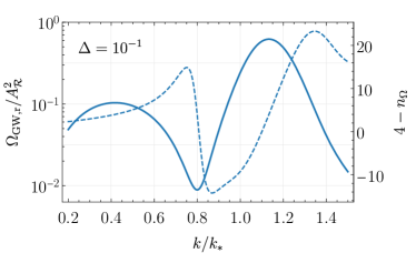
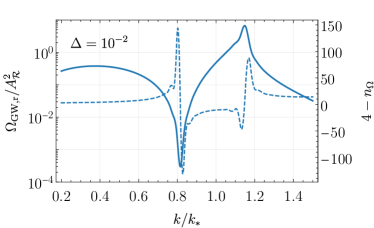
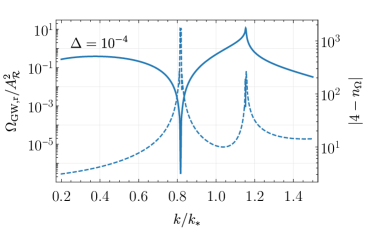
Figure 1: The dashed curves show the spectral tilt factor $4-n_{\Omega}$, the solid curves show the GW amplitude $\Omega_{\rm GW,r}/A_{\mathcal{R}}^{2}$.

The GW spectrum and this spectral tilt factor $n_{\Omega}$ as a function of $k$ are plotted in Fig. 1 for different choices of $\Delta$. The frequency profile of the stochastic gravitational wave spectrum induced at second order from scalar fluctuations can be understood analytically, at least for simple ansätze of the sourcing scalar spectrum. For example, for a delta-like scalar source, peaked at momentum $k\equiv k_{*}$, the resulting induced SGWB spectrum has a dip and goes to zero for $k/k_{\star}=\sqrt{2/3}$, and a pronounced resonant peak at $k/k_{\star}=\sqrt{4/3}$.

If the source scalar spectrum profile is narrow but not a delta-function, then the previous features are smoothed. Fig. 1 shows the SGWB induced by a log-normal peak, for different choices of the characteristic width. The technical reason for these features can be found in the convolution integrals that give the SGWB at second order: see e.g. [75, 76, 91] for important early works on the subject, as well as [77] for a recent systematic review. The features are due to interference and resonant effects among the scalar modes that source the GW background.

The spectrum is normalised against $A_{\mathcal{R}}^{2}$ because the latter quantity always results as overall coefficient in front of the induced $\Omega_{\rm GW}$ at second order (see also [75, 76, 91, 77]). It is customary to plot the GW frequency profile singling out such overall factor.

3.1.1 Inflationary models with peaked spectra

A number of inflationary models can produce a sufficiently narrow peak in the GW spectrum which can enhance the SGWB anisotropies by a factor of $\mathcal{O}(100)$ or more. Within single-field models, the curvature power spectrum has bounds in its growth rate (see e.g. [92, 93, 94, 95]) which restricts the steepness of the induced GW spectrum [74, 75, 76], and – consequently – how large $n_{\Omega}$ can be. In fact, we find that single-field scenarios can in general be well-represented by the $\Delta=10^{-1}$ case of Fig. 1. On the other hand, models with modified gravity [96], multiple fields [97, 98, 99, 100, 101], parametric resonance [102, 103, 104, 105] or particle production [106] may produce the narrow spectra corresponding to scenarios with $\Delta\leq 10^{-2}$. One should also mention models with non-standard kinetic terms, these too can support an enhanced GW spectrum, see e.g. [41, 42].

3.1.2 Other sources of peaked GW spectra

GW from non-inflationary sources, e.g. phase transitions [107], cosmic strings [108], can also produce peaked spectra although the enhancement from the tilt is typically of the same order as for a power-law spectrum. As an example, let us consider the SGWB produced from cosmological phase transitions. For these backgrounds, the sound wave contribution is generally larger than the other contributions and has a steeper spectral shape given by [109]

$$S(k,k_{*})=\left(\frac{k}{k_{*}}\right)^{3}\left(\frac{7}{4+3(k/k_{*})^{2}}\right)^{7/2}\,,$$ (3.5)

with

$$\Omega_{\rm GW}(k)=\Omega_{\rm GW}(k_{*})S(k,k_{*})\,,$$ (3.6)

where $\Omega_{\rm GW}(k_{*})$ is the GW amplitude at the peak wavenumber $k_{*}$. From Eq. (3.5) one can infer that the factor $(4-n_{\Omega}(k))$ appearing in the R.H.S. of Eq. (3.4) is $\mathcal{O}$(1). Thus, the enhancement in this case is much smaller than what GW sourced from peaks in the curvature power spectrum allow for. In the next section, we focus on the latter scenario and explore the observational consequences through an example of SIGW detectable at mHz scales.

3.2 LISA GW-PBH scenario

As a representative example, we consider a scenario in which the scalar induced GW spectrum can be detected by LISA [9]. For this, we take the peak of the log-normal power spectrum of Eq. (3.1) to correspond to a frequency within the LISA band $10^{-4}\text{ Hz}\leq f\leq 10^{-1}\text{ Hz}$. The relation between frequency and wavenumber is given by

$$\frac{k}{\text{Mpc}^{-1}}\simeq 6.5\times 10^{14}\frac{f}{\text{Hz}}\,.$$ (3.7)

The induced GW spectrum is plotted in the left panel of Fig. 2 for the parameter choice of table 1. Note that to avoid numerical artifacts arising in the calculations we have also smoothed the $\Omega_{\rm GW}$ spectrum near the peak using the peak width as the smoothing scale. The smoothed spectrum $\widetilde{\Omega}_{\rm GW}$ is defined as

$$\widetilde{\Omega}_{\rm GW}(f)=\frac{1}{2\Delta}\int_{fe^{-\Delta}}^{fe^{\Delta}}\Omega_{\rm GW}(f^{\prime})\,d\ln f^{\prime}\,.$$ (3.8)

$\Delta$	$10^{-2}$
$f_{*}$	$5\times 10^{-3}\,\rm Hz$
$k_{*}$	$3\times 10^{12}\,\rm Mpc^{-1}$
$A_{\mathcal{R}}$	$7.5\times 10^{-3}$

Table 1: Parameter choice for the LISA GW scenario.

The enhancement of the curvature power spectrum can also lead to the production of PBH and one ought to ensure that the scenario considered here is well within the region allowed by current constraints on the PBH abundance. The relation between PBH mass at formation and the comoving scale $k$ re-entering the horizon (during the radiation era) can be written as [110, 78],

$$M_{\rm PBH}\simeq 30M_{\odot}\left(\frac{\gamma}{0.2}\right)\left(\frac{g_{*}}{10.75}\right)^{-1/6}\left(\frac{2.9\times 10^{5}{\rm Mpc^{-1}}}{k}\right)^{2}\,.$$ (3.9)

For peak frequencies/wavenumbers relevant for LISA this leads to PBH with masses in the range $M_{\rm PBH}\sim\mathcal{O}(10^{-15}\text{ -- }10^{-12})M_{\odot}$ (see [111, 112] for a detailed analysis of the PBH-GW scenario for LISA). In our case the corresponding PBH abundance is shown in the right panel of Fig. 2 for $\Delta=10^{-2}$ along with the corresponding constraints, compiled using the tool provided in [113]. To calculate the mass function of PBH we have followed the method of ref. [114] which uses a simple Press-Schechter approach and accounts for the effects of critical collapse. The PBH mass function $f_{\rm PBH}(M)$ is defined as,

$$\frac{\Omega_{\rm PBH}}{\Omega_{\rm DM}}=\int f_{\rm PBH}(M)\,d\ln M\,,$$ (3.10)

where the L.H.S. denotes the total fraction of the dark matter density constituted by PBH. Note that the constraints shown in Fig. 2 are strictly valid only for a monochromatic mass function and for extended mass functions the constraints need to be calculated differently [116].

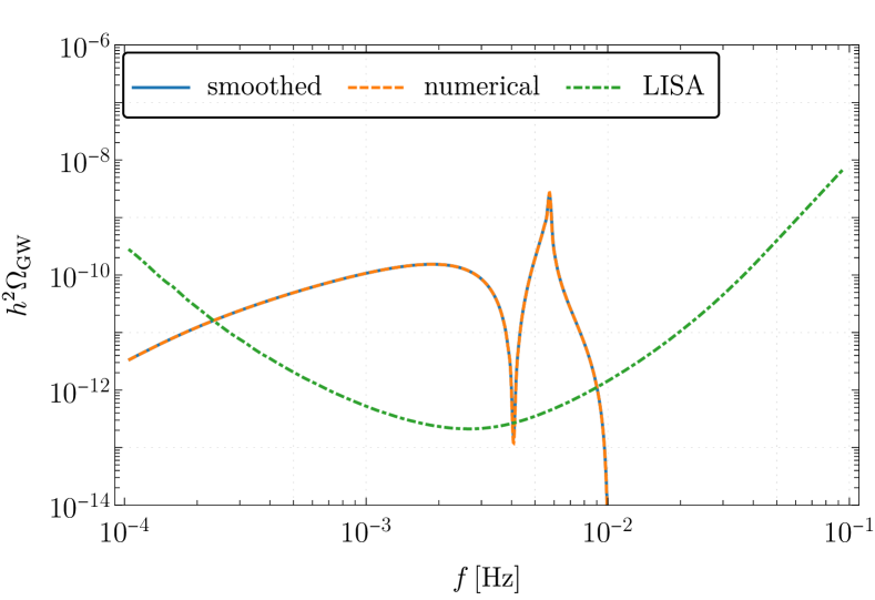
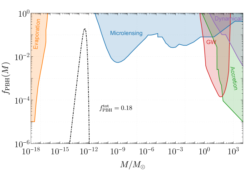
Figure 2: Left - The induced GW spectrum at LISA scales for the parameter choice given in table 1 and the smoothed spectrum defined in Eq. (3.8). The green dashed curve shows power-law integrated sensitivity curve for LISA [117] (see [118] for the updated sensitivity curves due to the impact of foregrounds and resolvable binaries). Right - The PBH abundance for the same values of the parameters plotted along with the constraints from microlensing [119, 120, 121, 122, 123, 124, 125], accretion [126, 127, 128, 129], GW [130], evaporation [131, 132, 133, 134, 135, 136, 137, 138, 139, 140, 141] and dynamical constraints [142, 143].

3.2.1 Angular power spectrum of GW anisotropies

We now calculate the angular power spectrum of the GW anisotropies for the LISA GW scenario of table 1. The angular power spectrum is defined as

$$\langle\Gamma_{\ell m}\Gamma_{\ell^{\prime}m^{\prime}}\rangle=\delta_{\ell\ell^{\prime}}\delta_{mm^{\prime}}C_{\ell}^{\Gamma}\,,$$ (3.11)

where we have assumed statistical isotropy. We denote by $C_{\ell}^{\rm GW}$ the angular power spectrum of $\delta_{\rm GW}$ which is related to the above quantity as follows,

$$C_{\ell}^{\rm GW}(k)=\left(4-n_{\Omega}(k)\right)^{2}C_{\ell}^{\Gamma}\,,$$ (3.12)

with $n_{\Omega}$ given by Eq. (3.4). In the left panel of Fig. 3 we plot the autocorrelation of the GW anisotropies and their cross-correlation with CMB temperature and E-mode polarisation anisotropies. We obtained the T and E transfer functions from CAMB [144]. Note that the propagation anisotropies of the CGWB quantity $\Gamma$ (Eq. (2.1.1)), and consequently $C_{\ell}^{\Gamma}$, are frequency independent. In the right panel, we show the frequency dependence of $C_{\ell}^{{\rm GW}}$ (for $\ell=2$) for the LISA GW scenario and for a flat spectrum of GW for comparison. For simplicity, we have only considered the SW contribution for GW anisotropies, Eq. (2.1.1), since this is the dominant contribution on large angular scales, and ignored the ISW term. These scales are the most relevant for the GW detectors under consideration here since these are limited by their angular resolution $\ell_{\rm max}\sim 15\text{--}30$ [145, 146, 147]. It is worth noting that this frequency dependence of the anisotropies arises for any SGWB that is different from a power-law ($n_{\Omega}=\rm const.$), whereas $C_{\ell}^{\Gamma}$ for the anisotropies from propagation is expected to be the same for all CGWB.

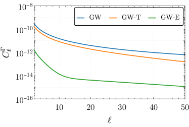
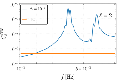
Figure 3: Left - Angular power spectrum of the GW anisotropies and their cross-correlation with CMB-T, E. Right - Frequency dependence of the angular power spectrum, for $\ell=2$, for the LISA model of table 1 (blue line) and for a flat spectrum (orange line) plotted in a frequency range where LISA has the highest sensitivity.

3.2.2 SNR of the anisotropies

In this section we show that the enhancement of anisotropies for a peaked spectrum can make these anisotropies easier to detect compared to the case of a standard power-law spectrum. A related phenomenon was recently pointed out in [148] for the case of kinematic anisotropies. For the purpose of this comparison, we consider a flat power-law spectrum with an amplitude such that the resulting SNR of the monopole is the same in the LISA range. We have verified that the results for a power law with a small non-zero spectral tilt $n_{\Omega}\sim\mathcal{O}(1)$ are similar so we do not show them separately. We plot the SNR for the individual multipoles in Fig.  4. Our results indicate that detecting the anisotropy is easier for a peaked spectrum than for a flat spectrum. We see that, although the $\ell=2$ is detectable with a LISA-Taiji network for the peaked spectra, it is not detectable for the flat spectra.

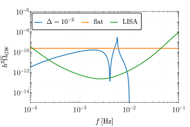
Figure 4: Left - $\Omega_{\rm GW}(f)$ plotted for the two spectra. Right - SNR of the individual multipoles with $T_{\rm obs}=3\rm\,years$.

The multipole SNR is defined as [149]

$$\text{SNR}_{\ell}^{2}=\int df\,C_{\ell}^{{\rm GW}}(f)\left(\frac{\Omega_{\rm GW}(f)}{\Omega^{\ell}_{{\rm GW},n}(f)}\right)^{2}\,,$$ (3.13)

where the quantity $\Omega^{\ell}_{{\rm GW},n}(f)$ is the effective angular sensitivity of the detector network to the $\ell-$th multipole. The quantity $\Omega_{\rm GW,n}^{\ell}(f)$ is defined as

$$\Omega_{\rm GW,n}^{\ell}(f)^{-1}\equiv T_{\rm obs}\sum_{AB}\left(\frac{2}{5}\right)^{2}\left(\frac{4\pi^{2}f^{3}}{3H_{0}^{2}}\right)^{-2}\frac{1}{N^{A}_{f}N^{B}_{f}}\frac{\sum_{m}|\mathcal{A}_{AB}^{\ell m}(f)|^{2}}{(2\ell+1)},$$ (3.14)

where $T_{\rm obs}$ is the time of observation, $N_{f}^{A}$ denotes the noise Power Spectral Density for detector $A$ and $\mathcal{A}^{\ell m}_{AB}$ the spherical harmonic transform of the antenna pattern for the detector pair $AB$.

We use the code schNell to compute $\Omega_{\rm GW,n}^{\ell}(f)$. Fig. 5 contains a plot of the quantity $\Omega_{\rm GW,n}^{\ell}(f)$ for LISA-Taiji [150] and for the BBO configuration with 4 constellations [24]. We include all LISA-Taiji cross-correlations as well correlations internal to both LISA and Taiji while for BBO we only consider cross-correlations among the different vertices. The addition of multiple detectors separated by large distances improves angular sensitivity compared to a single LISA-like constellation, e.g. see Fig. 9 of ref. [149] or Fig. 6 of ref. [145]. The noise curves for the various detectors can be found in [117] for LISA, [150] for Taiji and [151] for BBO.

Figure 5: Sensitivity of LISA-Taiji and BBO to the different multipoles of the SGWB as a function of frequency. The time of observation is taken to be 3 years for both plots.

SNR of the cross-correlation

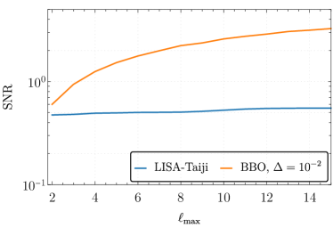
Figure 6: SNR of the cross-correlation between the GW anisotropies and the CMB-T, E mode anisotropies.

The SNR of the cross-correlation with the CMB-T, E anisotropies is defined as

$$\text{SNR}^{2}=\sum_{\ell=2}^{\ell_{\rm max}}\sum_{\rm X=T,E}(2\ell+1)\frac{\left(C^{\rm{X}\Gamma}\right)^{2}}{\left(C^{\rm{X}\Gamma}\right)^{2}+\left(C_{\ell}^{\Gamma}+N_{\ell}^{\Gamma}\right)C_{\ell}^{\rm X}}\,,$$ (3.15)

where the quantity $N_{\ell}^{\Gamma}$ is (for $\ell>0$)

$$N_{\ell}^{\Gamma}\equiv\left[\int df\frac{(4-n_{\Omega}(f))^{2}\overline{\Omega}_{\rm GW}(f)^{2}}{\Omega_{\rm GW,n}^{\ell}(f)^{2}}\right]^{-1}\,.$$ (3.16)

We plot the SNR in Fig. 6 as a function of $\ell_{\rm max}$ for observation by LISA-Taiji and BBO. For the representative example considered here, this cross-correlation will be detectable by a BBO-level GW detector but not with LISA-Taiji. The GW-T cross-correlation provides the entirety of the cross-correlation SNR while the GW-E contribution is negligible.

4 Conclusion

These are very exciting times for GW astronomy: observations of compact object mergers by LIGO-Virgo and KAGRA have already demonstrated its tremendous potential to shed light on stellar and black hole physics, late-time cosmology as well as general relativity itself.
The detection of a background resulting from the superposition of a large number of these astrophysical sources is also expected to happen in the near future. When it comes to a cosmological background, such as the one from inflation, detection will likely be more challenging and require space-based and future ground-based interferometers. The importance of detecting cosmological backgrounds cannot be understated. These are generated well before the CMB and thus provide access to the primordial universe at much earlier times than what is possible by electromagnetic observations alone.

Much like the CMB, the CGWB is predicted to be nearly isotropic with small fluctuations that may be inherent to the production mechanism itself or may arise due to propagation in a universe that is not perfectly homogeneous and isotropic.

In the first part of this paper we have reviewed two different approaches to derive these “propagation” anisotropies and shown how, under some simplifying assumptions, they can be related to each other once a careful choice of the GW initial conditions is performed.
We also pointed out how the adiabatic or isocurvature nature of the primordial perturbations affects this anisotropy through the intrinsic density fluctuation at the time when the GW start propagating. Whether or not a significant amplitude of isocurvature perturbations could be produced to noticeably alter the SGWB anisotropies while leaving the CMB unaffected is a subject that merits further investigation. We plan to address such matters in an upcoming work.

In the second part of this paper, we analysed the propagation anisotropy spectrum of SGWB sourced at second order in the curvature perturbation. We saw that if the primordial curvature power spectrum is sharply peaked around some scales, as is possible in scenarios of PBH production, the SGWB anisotropies can be enhanced by a factor $\sim\mathcal{O}(10\text{--}100)$ relative to those of a power-law SGWB spectrum. This enhancement arises due to the fact that the multiplicative factor $(4-n_{\Omega})$ in the definition of $\delta_{\rm GW}$ in Eq. (3.4) becomes large if the SGWB spectrum is sharply peaked.
Through the representative example of a scalar induced SGWB detectable at mHz frequencies, we showed that even though this enhancement only affects certain scales, it can nevertheless make these anisotropies easier to detect relative to those of a standard power-law spectrum. For this representative example, we demonstrated the capability of a LISA-Taiji network to detect the $\ell=2$ multipole as well as that of BBO to detect the cross-correlation with CMB anisotropies. Larger values of the SGWB monopole would naturally increase the detectability of these anisotropies, as would the improved sensitivity and angular resolution of futuristic detector networks like BBO/DECIGO.
We also considered SGWB from other sources which may exhibit a peaked spectral shape. We find that in a representative case (see section 3.1.2) the enhancement of the anisotropies is small compared to the PBH scenario mentioned above. Irrespective of whether the enhancement is significant or not, the distinct frequency dependence of the SGWB anisotropies for such spectra could possibly be exploited to separate them from the anisotropies associated with other CGWB or even SGWB of astrophysical origin. This idea has been previously used for the CMB to subtract the contribution from foreground sources. A dedicated analysis of its feasibility for GW is also worth pursuing and would bring us one step closer to the detection of these GW anisotropies.

Acknowledgments

M.F. would like to acknowledge support from the “Atracción de Talento” grant 2019-T1/TIC15784, his work is partially supported by the Spanish Research Agency (Agencia Estatal de Investigación) through the Grant IFT Centro de Excelencia Severo Ochoa No CEX2020-001007-S, funded by MCIN/AEI/10.13039/501100011033. GT is partially funded by the STFC grant ST/T000813/1. For the purpose of open access, the authors have applied a Creative Commons Attribution (CC BY) licence to any Author Accepted Manuscript version arising.

Appendix A Boltzmann equation in $\zeta$-gauge

In this Appendix, we provide additional details relevant to the calculations of Sec. 2.2 and then briefly review the original computation of ref. [48].

To begin with, let $\lambda$ be the affine parameter along the graviton geodesic. The graviton 4-momentum is then $P^{\mu}=dx/d\lambda$. Let us express this in terms of the quantity $p$ defined as $p^{2}\equiv g_{ij}P^{i}P^{j}$, and $\hat{n}$, the unit vector along the GW direction. To this end, we first write $P^{i}=C\hat{n}$, where $C$ can be determined in terms of $p$ as,

$$p^{2} =g_{ij}P^{i}P^{j}=a^{2}(1+2\zeta)C^{2}\delta_{ij}n^{i}n^{j}$$

$$\implies C=\frac{p}{a}(1-\zeta)\,.$$ (A.1)

Next, using $g_{\mu\nu}P^{\mu}P^{\nu}=0$ we find,

$$P^{0}=\frac{p}{a}\left(1-\frac{2}{5aH}\partial_{i}\zeta n^{i}\right)\,.$$ (A.2)

To solve the Boltzmann equation (2.2) we need to calculate $dq/d\eta$ with $q=|\vec{p}|a$. Using Eqs. (A) and (A.2) one finds $P_{0}=-q$. Thus, it only remains to solve the geodesic equation for $P_{0}$. This is given by [154],

$$\frac{dP_{0}}{d\lambda}=\frac{1}{2}\partial_{0}g_{\alpha\beta}P^{\alpha}P^{\beta}\,.$$ (A.3)

Using the fact that $d/d\lambda=P^{0}d/d\eta$ one can re-write the above equation as

$$P^{0}\frac{dP_{0}}{d\eta}=\frac{1}{2}\partial_{0}g_{\alpha\beta}P^{\alpha}P^{\beta}.$$ (A.4)

To simplify things further, we can work with the re-scaled metric without the scale factor which we denote by $\tilde{g}_{\mu\nu}$, i.e. $g_{\mu\nu}=a^{2}\tilde{g}_{\mu\nu}$. The null geodesics remain the same; the affine parameters and the tangent vectors in the rescaled metric, on the other hand, are respectively given by $d\tilde{\lambda}=a^{-2}d\lambda$ and $\tilde{P}_{\mu}=a^{2}P^{\mu}$ [155]. One also finds $P_{\mu}=\tilde{P}_{\mu}$. Using these relations the geodesic equation reads,

$$\frac{d\tilde{P}_{0}}{d\eta}=-\frac{2}{5}\tilde{P}^{0}\left(\frac{a}{a^{\prime}}\right)^{\prime}\partial_{i}\zeta n^{i}\,,$$ (A.5)

where the prime denotes a partial derivative with respect to conformal time. Using $P_{0}=\tilde{P_{0}}$ and re-writing the above expression using the quantities defined in the original metric $g_{\mu\nu}$, one obtains at linear order in $\zeta$,

$$\frac{dP_{0}}{d\eta} =-\frac{1}{5}a^{2}P^{0}\,\partial_{i}\zeta n^{i}$$

$$=-\frac{1}{5}q\,\partial_{i}\zeta n^{i}\,.$$ (A.6)

The Boltzmann equation then becomes

$$\frac{df}{d\eta}=\frac{\partial f}{\partial\eta}+\frac{\partial f}{\partial x^{i}}n^{i}+\frac{1}{5}q\partial_{i}\zeta n^{i}\frac{\partial f}{\partial q}$$ (A.7)

(Eq. (2.30) of the main text). Upon expanding the distribution function into a zeroth order term plus perturbations,

$$f(\eta,\vec{x},q,\hat{n})=\bar{f}(q)-q\frac{\partial\bar{f}}{\partial q}\Gamma(\eta,\vec{x},q,\hat{n})\,,$$ (A.8)

the Boltzmann equation at first order reads,

$$\frac{\partial\Gamma}{\partial\eta}+n^{i}\frac{\partial\Gamma}{\partial x^{i}}=\frac{1}{5}\frac{\partial\zeta}{\partial x^{i}}n^{i}\,.$$ (A.9)

In Fourier space, one finds

$$\frac{\partial\Gamma_{k}}{\partial\eta}+ik\mu\Gamma_{k}=\frac{ik\mu}{5}\zeta_{k}\,,$$ (A.10)

with $\mu\equiv\hat{k}\cdot\hat{n}$. This can be solved to give

$$\Gamma_{k}(\eta)=e^{ik\mu(\eta_{\rm in}-\eta)}\left[\Gamma_{k}(\eta_{\rm in},q,\hat{n})-\frac{1}{5}\zeta_{k}(\eta_{\rm in})\right]\,,$$ (A.11)

which is Eq. (2.32) in Fourier space.

We also provide here the original derivation of ref. [48]. Starting from Eq. (A.5) and using the fact that the derivative along the geodesic can be written as

$$\frac{d}{d\eta}=\frac{\partial}{\partial\eta}+n^{i}\partial_{i}\,,$$ (A.12)

one obtains [156]

$$\frac{dP_{0}}{d\eta}=-\frac{2}{5}P^{0}\left(\frac{a}{a^{\prime}}\right)^{\prime}\frac{d}{d\eta}\zeta\,.$$ (A.13)

At zeroth order $P_{0}=-P^{0}$ and one finds,

$$P_{0}(\eta)=P_{0}(\eta_{\rm i})\left[1+\frac{1}{5}\left(\zeta(\eta,\mathbf{x})-\zeta(\eta_{\rm i},\mathbf{x}_{i})\right)\right]\,,$$ (A.14)

where $\vec{x}_{0}=\vec{x}_{i}+(\eta_{0}-\eta_{i})\hat{n}$. Equivalently, we can write for the comoving momentum $q$,

$$\frac{q}{q_{i}}=\left[1+\frac{1}{5}\left(\zeta(\eta,\vec{x})-\zeta(\eta_{\rm i},\vec{x}_{i})\right)\right].$$ (A.15)

In this case one obtains a SGWB anisotropy equal to:

$$\delta_{\rm GW}(q,\hat{n}) =\frac{1}{5}\zeta(\eta_{i},\vec{x}_{i})\frac{\partial\ln\bar{f}(q)}{\partial\ln q}$$ (A.16)

(Eq. (2.34) of the main text). Note the implicit assumption here that there is no initial perturbation to the distribution function, i.e. $f(\eta_{i},\vec{x}_{i})=\bar{f}(\eta_{i})$, which is valid for adiabatic primordial perturbations when working in the uniform matter density gauge (see the discussion in Sec. 2.2.). The curvature perturbation at the observer’s position can also be ignored since it only contributes to the monopole. Ref. [48] considers the case of GW from single-field slow-roll inflation, with a distribution function $\bar{f}(q)\propto(q_{0}/q)^{2(\nu+1+\epsilon)}$. Here $q_{0}$ is a reference frequency, $\epsilon$ the standard slow-roll parameter during inflation and $\nu\equiv 2/(1+3\mathsf{w})$ with $\mathsf{w}$ evaluated at the time when the GW mode re-enters the horizon. Evaluating the SGWB anisotropy in terms of these quantities one arrives at [48],

$$\delta_{\rm GW}(q,\hat{n})=-\frac{2}{5}(\nu+1+\epsilon)\zeta(\eta_{i},\vec{x}_{i})\,.$$ (A.17)

References

- [1] LIGO Scientific, Virgo collaboration, B. P. Abbott et al., Search for the isotropic stochastic background using data from Advanced LIGO’s second observing run, Phys. Rev. D 100 (2019) 061101, [1903.02886].
- [2] KAGRA, Virgo, LIGO Scientific collaboration, R. Abbott et al., Upper limits on the isotropic gravitational-wave background from Advanced LIGO and Advanced Virgo’s third observing run, Phys. Rev. D 104 (2021) 022004, [2101.12130].
- [3] NANOGrav collaboration, Z. Arzoumanian et al., The NANOGrav 12.5 yr Data Set: Search for an Isotropic Stochastic Gravitational-wave Background, Astrophys. J. Lett. 905 (2020) L34, [2009.04496].
- [4] T. Regimbau, The astrophysical gravitational wave stochastic background, Res. Astron. Astrophys. 11 (2011) 369–390, [1101.2762].
- [5] C. Caprini and D. G. Figueroa, Cosmological Backgrounds of Gravitational Waves, Class. Quant. Grav. 35 (2018) 163001, [1801.04268].
- [6] M. Guzzetti, N. Bartolo, M. Liguori and S. Matarrese, Gravitational waves from inflation, Riv. Nuovo Cim. 39 (2016) 399–495, [1605.01615].
- [7] M. Punturo et al., The Einstein Telescope: A third-generation gravitational wave observatory, Class. Quant. Grav. 27 (2010) 194002.
- [8] D. Reitze et al., Cosmic Explorer: The U.S. Contribution to Gravitational-Wave Astronomy beyond LIGO, Bull. Am. Astron. Soc. 51 (2019) 035, [1907.04833].
- [9] P. Amaro-Seoane, H. Audley, S. Babak, J. Baker, E. Barausse, P. Bender et al., Laser interferometer space antenna, 1702.00786.
- [10] W.-R. Hu and Y.-L. Wu, The Taiji Program in Space for gravitational wave physics and the nature of gravity, Natl. Sci. Rev. 4 (2017) 685–686.
- [11] W. Giarè, F. Renzi and A. Melchiorri, Higher-Curvature Corrections and Tensor Modes, Phys. Rev. D 103 (2021) 043515, [2012.00527].
- [12] N. Bartolo and G. Orlando, Parity breaking signatures from a Chern-Simons coupling during inflation: the case of non-Gaussian gravitational waves, JCAP 07 (2017) 034, [1706.04627].
- [13] C. Burrage, C. de Rham, D. Seery and A. J. Tolley, Galileon inflation, JCAP 01 (2011) 014, [1009.2497].
- [14] A. J. Tolley and M. Wyman, The Gelaton Scenario: Equilateral non-Gaussianity from multi-field dynamics, Phys. Rev. D 81 (2010) 043502, [0910.1853].
- [15] Planck collaboration, P. A. R. Ade et al., Planck 2015 results. XX. Constraints on inflation, 1502.02114.
- [16] Planck collaboration, Y. Akrami et al., Planck 2018 results. X. Constraints on inflation, 1807.06211.
- [17] BICEP, Keck collaboration, P. A. R. Ade et al., Improved Constraints on Primordial Gravitational Waves using Planck, WMAP, and BICEP/Keck Observations through the 2018 Observing Season, Phys. Rev. Lett. 127 (2021) 151301, [2110.00483].
- [18] M. Tristram et al., Improved limits on the tensor-to-scalar ratio using BICEP and Planck, 2112.07961.
- [19] CMB-S4 collaboration, K. Abazajian et al., CMB-S4: Forecasting Constraints on Primordial Gravitational Waves, 2008.12619.
- [20] Simons Observatory collaboration, P. Ade et al., The Simons Observatory: Science goals and forecasts, JCAP 02 (2019) 056, [1808.07445].
- [21] LiteBIRD collaboration, E. Allys et al., Probing Cosmic Inflation with the LiteBIRD Cosmic Microwave Background Polarization Survey, 2202.02773.
- [22] A. A. Starobinsky, A New Type of Isotropic Cosmological Models Without Singularity, Phys. Lett. B91 (1980) 99–102.
- [23] A. Kehagias, A. Moradinezhad Dizgah and A. Riotto, Remarks on the Starobinsky model of inflation and its descendants, Phys. Rev. D 89 (2014) 043527, [1312.1155].
- [24] J. Crowder and N. J. Cornish, Beyond LISA: Exploring future gravitational wave missions, Phys. Rev. D 72 (2005) 083005, [gr-qc/0506015].
- [25] J. L. Cook and L. Sorbo, Particle production during inflation and gravitational waves detectable by ground-based interferometers, Phys. Rev. D 85 (2012) 023534, [1109.0022].
- [26] N. Barnaby, E. Pajer and M. Peloso, Gauge Field Production in Axion Inflation: Consequences for Monodromy, non-Gaussianity in the CMB, and Gravitational Waves at Interferometers, Phys. Rev. D 85 (2012) 023525, [1110.3327].
- [27] N. Barnaby, J. Moxon, R. Namba, M. Peloso, G. Shiu and P. Zhou, Gravity waves and non-Gaussian features from particle production in a sector gravitationally coupled to the inflaton, Phys. Rev. D 86 (2012) 103508, [1206.6117].
- [28] E. Dimastrogiovanni, M. Fasiello and T. Fujita, Primordial Gravitational Waves from Axion-Gauge Fields Dynamics, JCAP 01 (2017) 019, [1608.04216].
- [29] J. Garcia-Bellido, M. Peloso and C. Unal, Gravitational waves at interferometer scales and primordial black holes in axion inflation, JCAP 12 (2016) 031, [1610.03763].
- [30] B. Thorne, T. Fujita, M. Hazumi, N. Katayama, E. Komatsu and M. Shiraishi, Finding the chiral gravitational wave background of an axion-SU(2) inflationary model using CMB observations and laser interferometers, Phys. Rev. D 97 (2018) 043506, [1707.03240].
- [31] V. Domcke and K. Mukaida, Gauge Field and Fermion Production during Axion Inflation, JCAP 11 (2018) 020, [1806.08769].
- [32] L. Bordin, P. Creminelli, A. Khmelnitsky and L. Senatore, Light Particles with Spin in Inflation, JCAP 10 (2018) 013, [1806.10587].
- [33] L. Iacconi, M. Fasiello, H. Assadullahi, E. Dimastrogiovanni and D. Wands, Interferometer Constraints on the Inflationary Field Content, JCAP 03 (2020) 031, [1910.12921].
- [34] P. Campeti, E. Komatsu, D. Poletti and C. Baccigalupi, Measuring the spectrum of primordial gravitational waves with CMB, PTA and Laser Interferometers, JCAP 01 (2021) 012, [2007.04241].
- [35] L. Iacconi, M. Fasiello, H. Assadullahi and D. Wands, Small-scale Tests of Inflation, JCAP 12 (2020) 005, [2008.00452].
- [36] S. Endlich, A. Nicolis and J. Wang, Solid Inflation, JCAP 1310 (2013) 011, [1210.0569].
- [37] N. Bartolo, D. Cannone, A. Ricciardone and G. Tasinato, Distinctive signatures of space-time diffeomorphism breaking in EFT of inflation, JCAP 03 (2016) 044, [1511.07414].
- [38] A. Ricciardone and G. Tasinato, Primordial gravitational waves in supersolid inflation, Phys. Rev. D 96 (2017) 023508, [1611.04516].
- [39] M. Celoria, D. Comelli, L. Pilo and R. Rollo, Boosting GWs in Supersolid Inflation, JHEP 01 (2021) 185, [2010.02023].
- [40] M. Celoria, D. Comelli, L. Pilo and R. Rollo, Primordial Non-Gaussianity in Supersolid Inflation, 2103.10402.
- [41] M. Mylova, O. Özsoy, S. Parameswaran, G. Tasinato and I. Zavala, A new mechanism to enhance primordial tensor fluctuations in single field inflation, JCAP 12 (2018) 024, [1808.10475].
- [42] O. Ozsoy, M. Mylova, S. Parameswaran, C. Powell, G. Tasinato and I. Zavala, Squeezed tensor non-Gaussianity in non-attractor inflation, JCAP 09 (2019) 036, [1902.04976].
- [43] E. Dimastrogiovanni, M. Fasiello and G. Tasinato, Searching for Fossil Fields in the Gravity Sector, Phys. Rev. Lett. 124 (2020) 061302, [1906.07204].
- [44] P. Adshead, N. Afshordi, E. Dimastrogiovanni, M. Fasiello, E. A. Lim and G. Tasinato, Multimessenger Cosmology: correlating CMB and SGWB measurements, Phys. Rev. D 103 (2021) 023532, [2004.06619].
- [45] A. Malhotra, E. Dimastrogiovanni, M. Fasiello and M. Shiraishi, Cross-correlations as a Diagnostic Tool for Primordial Gravitational Waves, JCAP 03 (2021) 088, [2012.03498].
- [46] E. Dimastrogiovanni, M. Fasiello, A. Malhotra, P. D. Meerburg and G. Orlando, Testing the early universe with anisotropies of the gravitational wave background, JCAP 02 (2022) 040, [2109.03077].
- [47] E. Dimastrogiovanni, M. Fasiello and L. Pinol, Primordial Stochastic Gravitational Wave Background Anisotropies: in-in Formalization and Applications, 2203.17192.
- [48] V. Alba and J. Maldacena, Primordial gravity wave background anisotropies, JHEP 03 (2016) 115, [1512.01531].
- [49] C. R. Contaldi, Anisotropies of Gravitational Wave Backgrounds: A Line Of Sight Approach, Phys. Lett. B 771 (2017) 9–12, [1609.08168].
- [50] N. Bartolo, D. Bertacca, S. Matarrese, M. Peloso, A. Ricciardone, A. Riotto et al., Anisotropies and non-Gaussianity of the Cosmological Gravitational Wave Background, Phys. Rev. D 100 (2019) 121501, [1908.00527].
- [51] N. Bartolo, D. Bertacca, S. Matarrese, M. Peloso, A. Ricciardone, A. Riotto et al., Characterizing the cosmological gravitational wave background: Anisotropies and non-Gaussianity, Phys. Rev. D 102 (2020) 023527, [1912.09433].
- [52] V. Domcke, R. Jinno and H. Rubira, Deformation of the gravitational wave spectrum by density perturbations, JCAP 06 (2020) 046, [2002.11083].
- [53] M. Geller, A. Hook, R. Sundrum and Y. Tsai, Primordial Anisotropies in the Gravitational Wave Background from Cosmological Phase Transitions, Phys. Rev. Lett. 121 (2018) 201303, [1803.10780].
- [54] S. Kumar, R. Sundrum and Y. Tsai, Non-Gaussian stochastic gravitational waves from phase transitions, JHEP 11 (2021) 107, [2102.05665].
- [55] Y. Li, F. P. Huang, X. Wang and X. Zhang, Anisotropy of phase transition gravitational wave, 2112.01409.
- [56] S. Olmez, V. Mandic and X. Siemens, Anisotropies in the Gravitational-Wave Stochastic Background, JCAP 07 (2012) 009, [1106.5555].
- [57] S. Kuroyanagi, K. Takahashi, N. Yonemaru and H. Kumamoto, Anisotropies in the gravitational wave background as a probe of the cosmic string network, Phys. Rev. D 95 (2017) 043531, [1604.00332].
- [58] A. C. Jenkins and M. Sakellariadou, Anisotropies in the stochastic gravitational-wave background: Formalism and the cosmic string case, Phys. Rev. D 98 (2018) 063509, [1802.06046].
- [59] R.-G. Cai, Z.-K. Guo and J. Liu, A New Picture of Cosmic String Evolution and Anisotropic Stochastic Gravitational-Wave Background, 2112.10131.
- [60] L. Valbusa Dall’Armi, A. Ricciardone, N. Bartolo, D. Bertacca and S. Matarrese, Imprint of relativistic particles on the anisotropies of the stochastic gravitational-wave background, Phys. Rev. D 103 (2021) 023522, [2007.01215].
- [61] M. Braglia and S. Kuroyanagi, Probing prerecombination physics by the cross-correlation of stochastic gravitational waves and CMB anisotropies, Phys. Rev. D 104 (2021) 123547, [2106.03786].
- [62] A. Ricciardone, L. V. Dall’Armi, N. Bartolo, D. Bertacca, M. Liguori and S. Matarrese, Cross-Correlating Astrophysical and Cosmological Gravitational Wave Backgrounds with the Cosmic Microwave Background, Phys. Rev. Lett. 127 (2021) 271301, [2106.02591].
- [63] G. Cusin, C. Pitrou and J.-P. Uzan, Anisotropy of the astrophysical gravitational wave background: Analytic expression of the angular power spectrum and correlation with cosmological observations, Phys. Rev. D 96 (2017) 103019, [1704.06184].
- [64] G. Cusin, I. Dvorkin, C. Pitrou and J.-P. Uzan, First predictions of the angular power spectrum of the astrophysical gravitational wave background, Phys. Rev. Lett. 120 (2018) 231101, [1803.03236].
- [65] A. C. Jenkins, M. Sakellariadou, T. Regimbau and E. Slezak, Anisotropies in the astrophysical gravitational-wave background: Predictions for the detection of compact binaries by LIGO and Virgo, Phys. Rev. D 98 (2018) 063501, [1806.01718].
- [66] A. C. Jenkins, R. O’Shaughnessy, M. Sakellariadou and D. Wysocki, Anisotropies in the astrophysical gravitational-wave background: The impact of black hole distributions, Phys. Rev. Lett. 122 (2019) 111101, [1810.13435].
- [67] A. C. Jenkins and M. Sakellariadou, Shot noise in the astrophysical gravitational-wave background, Phys. Rev. D 100 (2019) 063508, [1902.07719].
- [68] G. Cusin, I. Dvorkin, C. Pitrou and J.-P. Uzan, Stochastic gravitational wave background anisotropies in the mHz band: astrophysical dependencies, Mon. Not. Roy. Astron. Soc. 493 (2020) L1–L5, [1904.07757].
- [69] G. Cusin, I. Dvorkin, C. Pitrou and J.-P. Uzan, Properties of the stochastic astrophysical gravitational wave background: astrophysical sources dependencies, Phys. Rev. D 100 (2019) 063004, [1904.07797].
- [70] D. Bertacca, A. Ricciardone, N. Bellomo, A. C. Jenkins, S. Matarrese, A. Raccanelli et al., Projection effects on the observed angular spectrum of the astrophysical stochastic gravitational wave background, Phys. Rev. D 101 (2020) 103513, [1909.11627].
- [71] C. Pitrou, G. Cusin and J.-P. Uzan, Unified view of anisotropies in the astrophysical gravitational-wave background, Phys. Rev. D 101 (2020) 081301, [1910.04645].
- [72] G. Capurri, A. Lapi, C. Baccigalupi, L. Boco, G. Scelfo and T. Ronconi, Intensity and anisotropies of the stochastic Gravitational Wave background from merging compact binaries in galaxies, 2103.12037.
- [73] N. Bellomo, D. Bertacca, A. C. Jenkins, S. Matarrese, A. Raccanelli, T. Regimbau et al., CLASS_GWB: robust modeling of the astrophysical gravitational wave background anisotropies, 2110.15059.
- [74] S. Matarrese, S. Mollerach and M. Bruni, Second order perturbations of the Einstein-de Sitter universe, Phys. Rev. D 58 (1998) 043504, [astro-ph/9707278].
- [75] K. N. Ananda, C. Clarkson and D. Wands, The Cosmological gravitational wave background from primordial density perturbations, Phys. Rev. D 75 (2007) 123518, [gr-qc/0612013].
- [76] D. Baumann, P. J. Steinhardt, K. Takahashi and K. Ichiki, Gravitational Wave Spectrum Induced by Primordial Scalar Perturbations, Phys. Rev. D 76 (2007) 084019, [hep-th/0703290].
- [77] G. Domènech, Scalar Induced Gravitational Waves Review, Universe 7 (2021) 398, [2109.01398].
- [78] M. Sasaki, T. Suyama, T. Tanaka and S. Yokoyama, Primordial black holes—perspectives in gravitational wave astronomy, Class. Quant. Grav. 35 (2018) 063001, [1801.05235].
- [79] P. Auclair et al., Cosmology with the Laser Interferometer Space Antenna, 2204.05434.
- [80] R. A. Isaacson, Gravitational radiation in the limit of high frequency. i. the linear approximation and geometrical optics, Phys. Rev. 166 (Feb, 1968) 1263–1271.
- [81] C. W. Misner, K. S. Thorne and J. A. Wheeler, Gravitation. W. H. Freeman, San Francisco, 1973.
- [82] M. Maggiore, Gravitational wave experiments and early universe cosmology, Phys. Rept. 331 (2000) 283–367, [gr-qc/9909001].
- [83] L. R. W. Abramo, R. H. Brandenberger and V. F. Mukhanov, The Energy - momentum tensor for cosmological perturbations, Phys. Rev. D 56 (1997) 3248–3257, [gr-qc/9704037].
- [84] S. Dodelson, Modern Cosmology. Academic Press, Amsterdam, 2003.
- [85] P. Creminelli, C. Pitrou and F. Vernizzi, The CMB bispectrum in the squeezed limit, JCAP 11 (2011) 025, [1109.1822].
- [86] J. Hwang, T. Padmanabhan, O. Lahav and H. Noh, On the 1/3 factor in the CMB Sachs-Wolfe effect, Phys. Rev. D 65 (2002) 043005, [astro-ph/0107307].
- [87] A. Bodas and R. Sundrum, Primordial Clocks within Stochastic Gravitational Wave Anisotropies, 2205.04482.
- [88] L. Boubekeur, P. Creminelli, J. Norena and F. Vernizzi, Action approach to cosmological perturbations: the 2nd order metric in matter dominance, JCAP 08 (2008) 028, [0806.1016].
- [89] S. Pi and M. Sasaki, Gravitational Waves Induced by Scalar Perturbations with a Lognormal Peak, JCAP 09 (2020) 037, [2005.12306].
- [90] N. Bartolo, D. Bertacca, V. De Luca, G. Franciolini, S. Matarrese, M. Peloso et al., Gravitational wave anisotropies from primordial black holes, JCAP 02 (2020) 028, [1909.12619].
- [91] R. Saito and J. Yokoyama, Gravitational-Wave Constraints on the Abundance of Primordial Black Holes, Progress of Theoretical Physics 123 (May, 2010) 867–886, [0912.5317].
- [92] C. T. Byrnes, P. S. Cole and S. P. Patil, Steepest growth of the power spectrum and primordial black holes, JCAP 06 (2019) 028, [1811.11158].
- [93] P. Carrilho, K. A. Malik and D. J. Mulryne, Dissecting the growth of the power spectrum for primordial black holes, Phys. Rev. D 100 (2019) 103529, [1907.05237].
- [94] O. Özsoy and G. Tasinato, On the slope of the curvature power spectrum in non-attractor inflation, JCAP 04 (2020) 048, [1912.01061].
- [95] G. Tasinato, An analytic approach to non-slow-roll inflation, Phys. Rev. D 103 (2021) 023535, [2012.02518].
- [96] S. Pi, Y.-l. Zhang, Q.-G. Huang and M. Sasaki, Scalaron from -gravity as a heavy field, JCAP 05 (2018) 042, [1712.09896].
- [97] J. Garcia-Bellido, A. D. Linde and D. Wands, Density perturbations and black hole formation in hybrid inflation, Phys. Rev. D 54 (1996) 6040–6058, [astro-ph/9605094].
- [98] P. H. Frampton, M. Kawasaki, F. Takahashi and T. T. Yanagida, Primordial Black Holes as All Dark Matter, JCAP 04 (2010) 023, [1001.2308].
- [99] G. A. Palma, S. Sypsas and C. Zenteno, Seeding primordial black holes in multifield inflation, Phys. Rev. Lett. 125 (2020) 121301, [2004.06106].
- [100] J. Fumagalli, S. Renaux-Petel, J. W. Ronayne and L. T. Witkowski, Turning in the landscape: a new mechanism for generating Primordial Black Holes, 2004.08369.
- [101] M. Braglia, D. K. Hazra, F. Finelli, G. F. Smoot, L. Sriramkumar and A. A. Starobinsky, Generating PBHs and small-scale GWs in two-field models of inflation, JCAP 08 (2020) 001, [2005.02895].
- [102] C. Chen and Y.-F. Cai, Primordial black holes from sound speed resonance in the inflaton-curvaton mixed scenario, JCAP 10 (2019) 068, [1908.03942].
- [103] Y.-F. Cai, C. Chen, X. Tong, D.-G. Wang and S.-F. Yan, When Primordial Black Holes from Sound Speed Resonance Meet a Stochastic Background of Gravitational Waves, Phys. Rev. D 100 (2019) 043518, [1902.08187].
- [104] R.-G. Cai, Z.-K. Guo, J. Liu, L. Liu and X.-Y. Yang, Primordial black holes and gravitational waves from parametric amplification of curvature perturbations, JCAP 06 (2020) 013, [1912.10437].
- [105] C. Chen, X.-H. Ma and Y.-F. Cai, Dirac-Born-Infeld realization of sound speed resonance mechanism for primordial black holes, Phys. Rev. D 102 (2020) 063526, [2003.03821].
- [106] J. Fumagalli, S. Renaux-Petel and L. T. Witkowski, Oscillations in the stochastic gravitational wave background from sharp features and particle production during inflation, JCAP 08 (2021) 030, [2012.02761].
- [107] C. Caprini et al., Science with the space-based interferometer eLISA. II: Gravitational waves from cosmological phase transitions, JCAP 04 (2016) 001, [1512.06239].
- [108] P. Auclair et al., Probing the gravitational wave background from cosmic strings with LISA, JCAP 04 (2020) 034, [1909.00819].
- [109] A. Mazumdar and G. White, Review of cosmic phase transitions: their significance and experimental signatures, Rept. Prog. Phys. 82 (2019) 076901, [1811.01948].
- [110] J. Garcia-Bellido, M. Peloso and C. Unal, Gravitational Wave signatures of inflationary models from Primordial Black Hole Dark Matter, JCAP 09 (2017) 013, [1707.02441].
- [111] N. Bartolo, V. De Luca, G. Franciolini, A. Lewis, M. Peloso and A. Riotto, Primordial Black Hole Dark Matter: LISA Serendipity, Phys. Rev. Lett. 122 (2019) 211301, [1810.12218].
- [112] N. Bartolo, V. De Luca, G. Franciolini, M. Peloso, D. Racco and A. Riotto, Testing primordial black holes as dark matter with LISA, Phys. Rev. D 99 (2019) 103521, [1810.12224].
- [113] B. J. Kavanagh, bradkav/pbhbounds: Release version, Nov., 2019. 10.5281/zenodo.3538999.
- [114] C. T. Byrnes, M. Hindmarsh, S. Young and M. R. S. Hawkins, Primordial black holes with an accurate QCD equation of state, JCAP 08 (2018) 041, [1801.06138].
- [115] A. D. Gow, C. T. Byrnes, P. S. Cole and S. Young, The power spectrum on small scales: Robust constraints and comparing PBH methodologies, JCAP 02 (2021) 002, [2008.03289].
- [116] B. Carr, M. Raidal, T. Tenkanen, V. Vaskonen and H. Veermäe, Primordial black hole constraints for extended mass functions, Phys. Rev. D 96 (2017) 023514, [1705.05567].
- [117] T. L. Smith and R. Caldwell, LISA for Cosmologists: Calculating the Signal-to-Noise Ratio for Stochastic and Deterministic Sources, Phys. Rev. D 100 (2019) 104055, [1908.00546].
- [118] M. Lewicki and V. Vaskonen, Impact of LIGO-Virgo binaries on gravitational wave background searches, 2111.05847.
- [119] N. Smyth, S. Profumo, S. English, T. Jeltema, K. McKinnon and P. Guhathakurta, Updated Constraints on Asteroid-Mass Primordial Black Holes as Dark Matter, Phys. Rev. D 101 (2020) 063005, [1910.01285].
- [120] EROS-2 collaboration, P. Tisserand et al., Limits on the Macho Content of the Galactic Halo from the EROS-2 Survey of the Magellanic Clouds, Astron. Astrophys. 469 (2007) 387–404, [astro-ph/0607207].
- [121] D. Croon, D. McKeen, N. Raj and Z. Wang, Subaru-HSC through a different lens: Microlensing by extended dark matter structures, Phys. Rev. D 102 (2020) 083021, [2007.12697].
- [122] K. Griest, A. M. Cieplak and M. J. Lehner, Experimental Limits on Primordial Black Hole Dark Matter from the First 2 yr of Kepler Data, Astrophys. J. 786 (2014) 158, [1307.5798].
- [123] M. Oguri, J. M. Diego, N. Kaiser, P. L. Kelly and T. Broadhurst, Understanding caustic crossings in giant arcs: characteristic scales, event rates, and constraints on compact dark matter, Phys. Rev. D 97 (2018) 023518, [1710.00148].
- [124] H. Niikura, M. Takada, S. Yokoyama, T. Sumi and S. Masaki, Constraints on Earth-mass primordial black holes from OGLE 5-year microlensing events, Phys. Rev. D 99 (2019) 083503, [1901.07120].
- [125] Macho collaboration, R. A. Allsman et al., MACHO project limits on black hole dark matter in the 1-30 solar mass range, Astrophys. J. Lett. 550 (2001) L169, [astro-ph/0011506].
- [126] J. Manshanden, D. Gaggero, G. Bertone, R. M. T. Connors and M. Ricotti, Multi-wavelength astronomical searches for primordial black holes, JCAP 06 (2019) 026, [1812.07967].
- [127] P. Lu, V. Takhistov, G. B. Gelmini, K. Hayashi, Y. Inoue and A. Kusenko, Constraining Primordial Black Holes with Dwarf Galaxy Heating, Astrophys. J. Lett. 908 (2021) L23, [2007.02213].
- [128] P. D. Serpico, V. Poulin, D. Inman and K. Kohri, Cosmic microwave background bounds on primordial black holes including dark matter halo accretion, Phys. Rev. Res. 2 (2020) 023204, [2002.10771].
- [129] A. Hektor, G. Hütsi, L. Marzola, M. Raidal, V. Vaskonen and H. Veermäe, Constraining Primordial Black Holes with the EDGES 21-cm Absorption Signal, Phys. Rev. D 98 (2018) 023503, [1803.09697].
- [130] G. Hütsi, M. Raidal, V. Vaskonen and H. Veermäe, Two populations of LIGO-Virgo black holes, JCAP 03 (2021) 068, [2012.02786].
- [131] B. J. Carr, K. Kohri, Y. Sendouda and J. Yokoyama, New cosmological constraints on primordial black holes, Phys. Rev. D 81 (2010) 104019, [0912.5297].
- [132] S. Clark, B. Dutta, Y. Gao, L. E. Strigari and S. Watson, Planck Constraint on Relic Primordial Black Holes, Phys. Rev. D 95 (2017) 083006, [1612.07738].
- [133] M. Boudaud and M. Cirelli, Voyager 1 Further Constrain Primordial Black Holes as Dark Matter, Phys. Rev. Lett. 122 (2019) 041104, [1807.03075].
- [134] S. Clark, B. Dutta, Y. Gao, Y.-Z. Ma and L. E. Strigari, 21 cm limits on decaying dark matter and primordial black holes, Phys. Rev. D 98 (2018) 043006, [1803.09390].
- [135] B. Dasgupta, R. Laha and A. Ray, Neutrino and positron constraints on spinning primordial black hole dark matter, Phys. Rev. Lett. 125 (2020) 101101, [1912.01014].
- [136] W. DeRocco and P. W. Graham, Constraining Primordial Black Hole Abundance with the Galactic 511 keV Line, Phys. Rev. Lett. 123 (2019) 251102, [1906.07740].
- [137] R. Laha, Primordial Black Holes as a Dark Matter Candidate Are Severely Constrained by the Galactic Center 511 keV -Ray Line, Phys. Rev. Lett. 123 (2019) 251101, [1906.09994].
- [138] R. Laha, J. B. Muñoz and T. R. Slatyer, INTEGRAL constraints on primordial black holes and particle dark matter, Phys. Rev. D 101 (2020) 123514, [2004.00627].
- [139] R. Laha, P. Lu and V. Takhistov, Gas heating from spinning and non-spinning evaporating primordial black holes, Phys. Lett. B 820 (2021) 136459, [2009.11837].
- [140] A. K. Saha and R. Laha, Sensitivities on non-spinning and spinning primordial black hole dark matter with global 21 cm troughs, 2112.10794.
- [141] S. Mittal, A. Ray, G. Kulkarni and B. Dasgupta, Constraining primordial black holes as dark matter using the global 21-cm signal with X-ray heating and excess radio background, JCAP 03 (2022) 030, [2107.02190].
- [142] M. A. Monroy-Rodríguez and C. Allen, The end of the macho era, revisited: New limits on macho masses from halo wide binaries, The Astrophysical Journal 790 (Jul, 2014) 159, [1406.5169].
- [143] T. D. Brandt, Constraints on MACHO Dark Matter from Compact Stellar Systems in Ultra-Faint Dwarf Galaxies, Astrophys. J. Lett. 824 (2016) L31, [1605.03665].
- [144] A. Lewis, A. Challinor and A. Lasenby, Efficient computation of CMB anisotropies in closed FRW models, Astrophys. J. 538 (2000) 473–476, [astro-ph/9911177].
- [145] H. Kudoh and A. Taruya, Probing anisotropies of gravitational-wave backgrounds with a space-based interferometer: Geometric properties of antenna patterns and their angular power, Phys. Rev. D 71 (2005) 024025, [gr-qc/0411017].
- [146] D. Alonso, C. R. Contaldi, G. Cusin, P. G. Ferreira and A. I. Renzini, Noise angular power spectrum of gravitational wave background experiments, Phys. Rev. D 101 (2020) 124048, [2005.03001].
- [147] C. R. Contaldi, M. Pieroni, A. I. Renzini, G. Cusin, N. Karnesis, M. Peloso et al., Maximum likelihood map-making with the Laser Interferometer Space Antenna, Phys. Rev. D 102 (2020) 043502, [2006.03313].
- [148] G. Cusin and G. Tasinato, Doppler boosting the stochastic gravitational wave background, 2201.10464.
- [149] N. Bartolo et al., Probing Anisotropies of the Stochastic Gravitational Wave Background with LISA, 2201.08782.
- [150] W.-H. Ruan, C. Liu, Z.-K. Guo, Y.-L. Wu and R.-G. Cai, The LISA-Taiji network, Nature Astron. 4 (2020) 108–109, [2002.03603].
- [151] T. L. Smith and R. Caldwell, Sensitivity to a Frequency-Dependent Circular Polarization in an Isotropic Stochastic Gravitational Wave Background, Phys. Rev. D 95 (2017) 044036, [1609.05901].
- [152] M. Tegmark, CMB mapping experiments: A Designer’s guide, Phys. Rev. D 56 (1997) 4514–4529, [astro-ph/9705188].
- [153] M. Tegmark, D. J. Eisenstein, W. Hu and A. de Oliveira-Costa, Foregrounds and forecasts for the cosmic microwave background, Astrophys. J. 530 (2000) 133–165, [astro-ph/9905257].
- [154] V. Mukhanov, Physical Foundations of Cosmology. Cambridge University Press, Oxford, 2005.
- [155] R. M. Wald, General Relativity. Chicago Univ. Pr., Chicago, USA, 1984. 10.7208/chicago/9780226870373.001.0001.
- [156] V. Alba, Aspects of scale invariance in Physics and Biology. PhD thesis, Princeton U., 9, 2017.