Benefits of Feedforward for Model Predictive Airpath Control of Diesel Engines

Abstract

This paper investigates options to complement a diesel engine airpath feedback controller with a feedforward. The control objective is to track the intake manifold pressure and exhaust gas recirculation (EGR) rate targets by manipulating the EGR valve and variable geometry turbine (VGT) while satisfying state and input constraints. The feedback controller is based on rate-based Model Predictive Control (MPC) that provides integral action for tracking. Two options for the feedforward are considered one based on a look-up table that specifies the feedforward as a function of engine speed and fuel injection rate, and another one based on a (non-rate-based) MPC that generates dynamic feedforward trajectories. The controllers are designed and verified using a high-fidelity engine model in GT-Power and exploit a low-order rate-based linear parameter-varying (LPV) model for prediction which is identified from transient response data generated by the GT-Power model. It is shown that the combination of feedforward and feedback MPC has the potential to improve the performance and robustness of the control design. In particular, the feedback MPC without feedforward can lose stability at low engine speeds, while MPC-based feedforward results in the best transient response. Mechanisms by which feedforward is able to assist in stabilization and improve performance are discussed.

, , , ,

1 Introduction

In this paper, we consider an airpath control problem for a diesel engine with exhaust gas recirculation (EGR) and variable geometry turbocharging (VGT), and examine complementary characteristics and demonstrate the benefits of combining feedforward and feedback Model Predictive Control (MPC)-based loops. The feedback MPC loop relies on a rate-based (velocity form) formulation that results in an integral action for offset-free tracking. The feedforward MPC loop exploits the conventional (non-rate-based) MPC formulation.

In particular, we demonstrate that the feedforward MPC that provides the capability of dynamically shaping the input trajectories improves the transient response and tracking performance of the airpath control as compared to a more conventional feedforward implementation using an engine speed-engine fuel injection rate based look-up table. Furthermore, when operating point changes due to changes in engine speed and fuel injection rate, feedforward MPC helps maintain the trajectory in the region of attraction of the feedback MPC controller and avoid instabilities due to nonlinear behavior of the engine, thereby improving the robustness of the diesel airpath control.

Due to its importance for fuel economy improvements and emissions reduction (Van Nieuwstadt et al., 2000), improvements to the diesel airpath control have been a long-standing research topic in automotive control. Several MPC solutions have been proposed starting with Ortner and Del Re (2007). See, for instance, the paper by Huang et al. (2018) for the historical outlook and references. In particular, the use of switching (non-MPC based) control has been considered in Bengea et al. (2004) where both feedforward and feedback are switched as the engine is transitioning between different operating points in such a way as to maintain the trajectory in the region of attraction of each operating point. The combined feedforward-feedback MPC architecture for the airpath control has been considered in Liao-McPherson et al. (2020), and its investigation is continued in this paper.

The conclusion about feedforward abetting the stability of the closed-loop system is interesting as regularly feedforward is viewed as a form of an open-loop control and therefore not capable of providing stabilization, with notable exceptions of vibration control (Meerkov, 1980). In constrained control, the use of a sensorless feedforward command governor has been proposed by Garone et al. (2011) that, in principle, could be used to a similar effect, by restricting the trajectory to satisfy constraints informed by the region of attraction dependent on the feedforward.

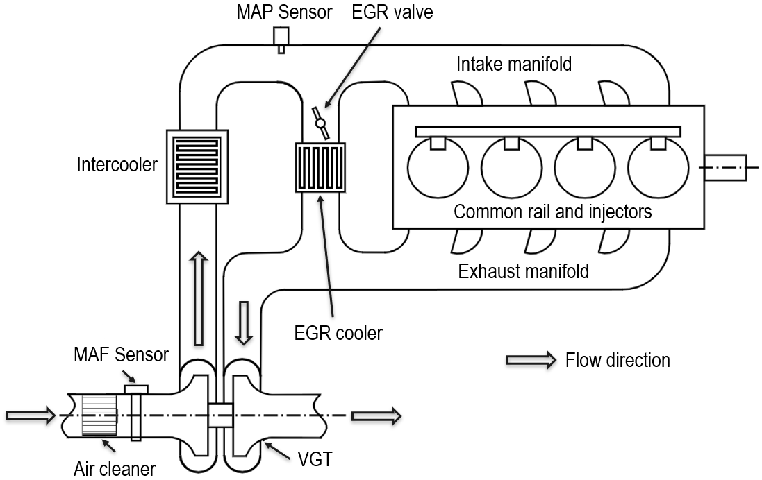
Figure 1: Schematic of a 4-cylinder diesel engine with EGR and VGT.

In this paper, the development of the combined feedforward and feedback MPC solution for the diesel airpath control is performed based on a high fidelity GT-Power engine model which is treated as a black box/surrogate for the engine. The operation-point dependent prediction models are identified based on input-output response data, and the overall model is defined in a linear parameter varying (LPV) form. We purposefully keep the model order low and in the input-output form (states are known outputs) to avoid the need to design and schedule a state observer. These developments are reported in Section 2. The feedforward and feedback MPC design is described in Section 3, where we also examine controller tuning issues. Concluding remarks are made in Section 5.

2 Diesel Engine Control Objectives, and Airpath Control-Oriented Modeling

2.1 Diesel Engine and Airpath Control Objectives

Figure 1 shows the schematics of a four-cylinder engine considered in this paper. The engine consists of a cylinder block, intake and exhaust manifolds, an exhaust gas recirculation (EGR) system, and a variable geometry turbocharger (VGT). The pressure in the intake manifold and the flow through the compressor of VGT are measured by a manifold absolute pressure (MAP) sensor and a mass airflow (MAF) flow sensor, respectively.

The engine operation point $\rho$ is defined by the engine speed ($N_{\tt e}$) and fuel injection rate ($w_{\tt inj}$) combination, $\rho=[N_{\tt e},w_{\tt inj}]^{\sf T}$, where $w_{\tt inj}$ corresponds to the sum of the pre-injection and main fuel injection rates.

The EGR valve controls the mass flow rate from the exhaust manifold into the intake manifold. The VGT controls the intake manifold pressure by varying the exhaust flow area and amount of energy extracted from the exhaust gas. The intake manifold pressure determines the mass flow rate into the engine cylinders. The gas flowing into the engine cylinders consists of air and exhaust gas. The EGR rate is defined as

$$\chi_{\tt egr}={w_{\tt egr}}/{(w_{\tt egr}+w_{\tt c})},$$ (1)

where $w_{\tt c}$ is the flow rate into the intake manifold through the compressor and intercooler and $w_{\tt egr}$ is the mass flow through the EGR valve into the intake manifold.

The objective of the airpath controller is to coordinate the EGR valve and VGT actuators to control the intake manifold pressure and EGR rate to the set-points (targets). These set-points are determined as functions of engine operating point (i.e., engine speed and fuel injection rate) in the engine calibration optimization phase to satisfy emissions and fuel efficiency requirements. Alternatively, these set-points and fuel injection rate could be adjusted by a supervisory controller, such as developed by Liao-McPherson et al. (2020), or an economic MPC controller, such as developed by Liao-McPherson et al. (2017). In the sequel, we assume that the intake manifold pressure and EGR rate set-points and the corresponding feedforward EGR valve and VGT positions have been computed and stored in interpolating look-up tables.

2.2 Diesel Airpath Control-Oriented Prediction Model

The MPC implementation requires a control-oriented prediction model. Following Zhang et al. (2022), we keep the prediction model as simple as possible. Hence the intake manifold pressure ($p_{\tt im}$) and EGR rate ($\chi_{\tt egr}$) are selected as the only model states of the system ($x$). The model inputs $u$ are EGR valve position (percent open) and VGT position (percent close). As the intake manifold pressure is measured and the EGR rate is estimated, this model structure eliminates the need for a state observer. With this approach, the engine constraints need to be remapped as functions of $p_{\tt im}$ and $\chi_{\tt egr}$ which can be done following the approach in Huang et al. (2016).

The control-oriented prediction model has an LPV form,

$$x_{k+1}-x_{k+1}^{\tt ss}(\rho_{k}) = A(\rho_{k})\left[x_{k}-x_{k}^{\tt ss}(\rho_{k})\right]$$ (2)

$$+ B(\rho_{k})\left[u_{k}-u_{k}^{\tt ss}(\rho_{k})\right]$$

$$+ B_{f}(\rho_{k})\left[w_{{\tt inj},k}-w_{{\tt inj}}^{\tt ss}(\rho_{k})\right],$$

where $k$ denote the discrete time, $\rho_{k}$ is the vector of engine speed and fuel injection rate at time instant $k$, $A,B:\mathbb{R}^{2}\to\mathbb{R}^{2\times 2}$, $x_{k}^{\tt ss},u_{k}^{\tt ss}:\mathbb{R}^{2}\to\mathbb{R}^{2}$ are mappings that determine equilibrium values of $x$ and $u$ corresponding to a given $\rho$, $B_{f}:~{}\mathbb{R}^{2}\to\mathbb{R}^{2\times 1}$, and $w_{\tt inj}^{\tt ss}(\rho)=\left[\begin{array}[]{cc}0&1\end{array}\right]\rho$.

The matrices $A(\rho)$ and $B(\rho)$ in (2) are computed by linear interpolation of the corresponding matrices of a finite set of $99$ models identified at pre-selected operating points ($\rho$) defined by $9$ values of the engine speed and $11$ values of fuel injection rate that cover the engine operating range. A high fidelity GT-Power diesel engine model has been used to generate input-output response data corresponding to small input perturbations; these data were then used for local model identification at each of the $99$ operating points. Note that the model (2) includes $w_{{\tt inj},k}$ as an extra additive input. This input has been added as including it improves the model match in transients. For validation results and further details on the LPV airpath model 2 development, see Zhang et al. (2022).

3 LPV-based MPC for Airpath Control

Our MPC design consists of a feedback (FB MPC) loop and a feedforward.

3.1 Rate-based Feedback (FB) MPC Loop

The FB MPC (Figure 2) exploits a rate-based prediction model as in Wang (2004); Pannocchia et al. (2015). The MPC design based on the rate-based model is able, under appropriate assumptions, to assure offset-free tracking Rawlings et al. (2017) and enhance closed-loop robustness and disturbance rejection capabilities. Such an approach has been also exploited in the earlier work by Huang et al. (2016).

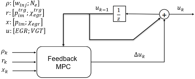
Figure 2: Schematic of FB airpath MPC loop. In the square box $z$ stands for the discrete time shift operator, i.e., $u_{k+1}=zu_{k}$.

The basic idea of the rate-based approach is to define rate variables, $\Delta x_{k}=x_{k}-x_{k-1},~{}\Delta u_{k}=u_{k}-u_{k-1},$ that correspond to the increments in the state and control variables. Then, assuming $\rho_{k}$ remains constant over the prediction horizon (it will be updated at the next control update instant), the prediction model (2) implies that

$$\Delta x_{k+1}=A(\rho_{k})\Delta x_{k}+B(\rho_{k})\Delta u_{k}.$$ (3)

Note that we set $w_{{\tt inj},k}-w_{\tt inj}^{\tt ss}(\rho_{k})-(w_{{\tt inj},k-1}-w_{\tt inj}^{\tt ss}(\rho_{k-1}))\\ =0$ in deriving (3) from (2) as in generating the FB MPC control signal, we assume $\rho_{k}$ remains constant over the prediction horizon. The latter assumption is adopted in much of the literature on engine and powertrain control with MPC. See Zhang et al. (2022) for further details.

We let $x_{j|k},$ $u_{j|k}$, $e_{j|k}=x_{j|k}-r_{k}$, where $r_{k}$ is the vector of the targets, denote the predicted state, control and tracking error values at time step $j$, $0\leq j\leq N$, over the prediction horizon when the prediction is made at the time step $k$. Then, to be able to impose constraints on $x_{j|k}$ and $u_{j|k}$ and compute MPC cost that penalizes the predicted tracking error, $e_{j|k}$, we define the augmented state vector, $\tiny{x_{j|k}^{\tt ext}=\left[\begin{array}[]{cccc}\Delta x_{j|k}^{\sf T},&e_{j|k}^{\sf T},&x_{j-1|k}^{\sf T},&u_{j-1|k}^{\sf T}\end{array}\right]^{\sf T}}$. The rate-based prediction model (3) then implies

$$x_{j+1|k}^{\tt ext}=\begin{bmatrix}A(\rho_{k})&0&0&0\\ A(\rho_{k})&\mathbb{I}_{n_{e}\times n_{e}}&0&0\\ \mathbb{I}_{n_{x}\times n_{x}}&0&\mathbb{I}_{n_{x}\times n_{x}}&0\\ 0&0&0&\mathbb{I}_{n_{u}\times n_{u}}\end{bmatrix}x_{j|k}^{\tt ext}$$

$$\qquad\qquad+\begin{bmatrix}B(\rho_{k})\\ B(\rho_{k})\\ 0\\ \mathbb{I}_{n_{u}\times n_{u}}\end{bmatrix}\Delta u_{j|k},$$ (4)

where $\Delta u_{j|k}$ is the control input in the extended system.

The FB MPC design is based on the solution of the following discrete time optimal control problem:

$$\min_{\Delta u_{0|k},...,\Delta u_{N-1|k},\epsilon_{k}}(x_{N|k}^{\tt ext})^{\sf T}P_{\infty|k}x_{N|k}^{\tt ext}+\\ \sum_{j=0}^{N-1}(x_{j|k}^{\tt ext})^{\sf T}Q^{\tt ext}x_{j|k}^{\tt ext}+\Delta u_{j|k}^{\sf T}R^{\tt ext}\Delta u_{j|k}+\mu\epsilon_{k}^{\sf T}\epsilon_{k}$$ (5a)

subject to

$$\Delta x_{0|k}=x_{k}-x_{k-1}$$ (5b)

$$e_{0|k}=x_{k}-r_{k}$$ (5c)

$$x_{-1|k}=x_{k-1}$$ (5d)

$$u_{-1|k}=u_{k-1}$$ (5e)

$$\Delta x_{j+1|k}=A(\rho_{k})\Delta x_{j|k}+B(\rho_{k})\Delta u_{j|k}$$ (5f)

$$e_{j+1|k}=A(\rho_{k})\Delta x_{j|k}+B(\rho_{k})\Delta u_{j|k}+e_{j|k}$$ (5g)

$$x_{j|k}=x_{j-1|k}+\Delta x_{j|k},j=1,\ldots,N,$$ (5h)

$$u_{j|k}=u_{j-1|k}+\Delta u_{j|k},j={0},\ldots,N-1,$$ (5i)

$$x_{min}-\epsilon_{k}\leq x_{j|k}\leq x_{max}+\epsilon_{k},j=1,\ldots,N,$$ (5j)

$$u_{min}\leq u_{j|k}\leq u_{max},j=0,\ldots,N-1,$$ (5k)

where $N$ is the prediction horizon, $Q^{\tt ext}\succeq 0$ and $R^{\tt ext}\succ 0$ are state and control weighting matrices, with $Q^{\tt ext}$ chosen so that $\tiny{(x_{j|k}^{\tt ext})^{\sf T}Q^{\tt ext}x_{j|k}^{\tt ext}=e_{j|k}^{\sf T}Q_{e}e_{j|k}}$, and $\epsilon_{k}$ is the slack variable introduced to avoid infeasibility of the state constraints.

The matrix $P_{\infty|k}\succeq 0$ imposes the terminal penalty on $\Delta x_{N|k}$ and $e_{N|k}$ states; such a terminal penalty is beneficial to ensure local closed-loop stability (when constraints are inactive with the engine operating near the set-point). To compute $P_{\infty|k}$, we first compute a matrix $\tilde{P}_{\infty|k}$ by solving the discrete algebraic Riccati equation (DARE) corresponding to the model for the evolution of just $\Delta x_{j|k}$ and $e_{j|k}$ states for which the dynamics ($A$) and input ($B$) matrices have the form,

$$\begin{bmatrix}A(\rho_{k})&0\\ A(\rho_{k})&\mathbb{I}_{n_{e}\times n_{e}}\end{bmatrix},\begin{bmatrix}B(\rho_{k})\\ B(\rho_{k})\end{bmatrix},$$ (6)

while the state and control weighting matrices are given by

$$\begin{bmatrix}0&0\\ 0&Q_{e}\end{bmatrix},R^{\tt ext}.$$ (7)

The terminal penalty matrix can be computed for a discrete set of values of $\rho$ on a chosen mesh and then interpolated element by element.

Numerically, (5) reduces to a quadratic programming (QP) problem. The first element of the optimal control sequence, $\Delta u_{0|k}^{*}$ then informs the FB MPC control signal according to the relation, $u_{k}=u_{k-1}+\Delta u_{0|k}^{*}$.

While the changes in the dynamic characteristics of the engine response across the engine operating range are captured by our LPV prediction model, we have also found in Zhang et al. (2022) that the closed-loop performance can be further improved by varying the weights $Q_{e}$ and $R^{\tt ext}$ in (5). To make the tuning process more tractable, we chose to group multiple operating points into regions and then tune the weighting matrices with the restriction that $Q_{e}$ (i.e., $Q^{\tt ext}$) and $R^{\tt ext}$ are the same for all operating points in a given region. In our implementation, we defined seven regions as a function of $N_{\tt e}$, $w_{\tt inj}$ and $\chi_{\tt egr}$, as shown in Figure 3. Note that the values of $N_{\tt e}$, $w_{\tt inj}$ and $\chi_{\tt egr}$ are categorized using qualitative “high” and “low” terms to protect the OEM proprietary data.

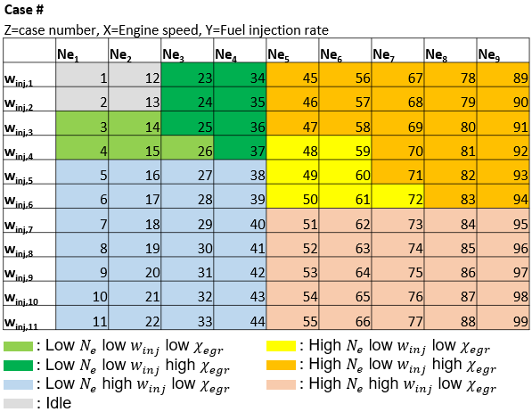
Figure 3: Seven regions defined as a function of $N_{\tt e}$, $w_{\tt inj}$ and $\chi_{\tt egr}$, to simplify the MPC tuning process with the same $Q^{ext}$ and $R^{ext}$ pair used in each region.

Figure 4 illustrates closed-loop response to steps in $w_{\tt inj}$ followed by ramps in $N_{\tt e}$ with the fully tuned FB MPC co-simulated with the GT-Power engine model through the Simulink interface. In these and subsequent simulations, we use the sampling period of $20$ ms and prediction horizon of $1$ s. The GT-Power simulation is configured to provide cycle averaged signals. The package mpctools developed by Risbeck and Rawlings (2016) is used for the numerical solution of MPC problem. The set-points are tracked with zero steady-state error and the overshoot and settling time of $p_{\tt im}$ are within the acceptable range ($1.5$ s). However, the response of $\chi_{\tt egr}$ to a step-change in $w_{\tt inj}$ has an undershoot and the tracking error is large in transients. The transient response can be made faster with a more aggressive tuning, however, in this case, it starts exhibiting larger overshoot and oscillations as is typical of controllers with integral action.

While the capability to improve closed-loop transient response by tuning of FB MPC is limited, there is an alternative route which is to exploit feedforward. This is further considered in the next section.

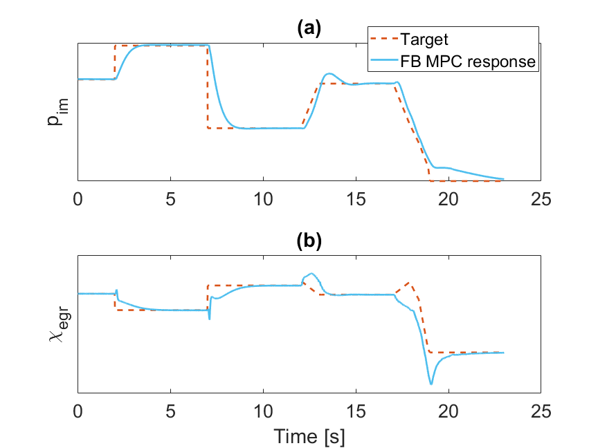
Figure 4: Example of (a) $p_{\tt im}$ and (b) $\chi_{\tt egr}$ trajectory tracking with FB MPC in response to steps in $w_{\tt inj}$ followed by ramps in $N_{\tt e}$.

3.2 Combination of Feedforward Look-up Table and FB MPC

Frequently, the engine control strategy involves a combination of feedforward and feedback. A feedback controller with an integral action alone is capable of eliminating the steady-state error, but its response can be slow. The combination of the feedforward and feedback can produce a faster action by the actuators and improve transient response.

In the case of our diesel engine, the simplest feedforward consists of steady-state EGR valve and VGT positions, consistent with $p_{\tt im}$ and $\chi_{\tt egr}$ set-points (and with given engine speed and fuel injection rate values) in steady-state, and aggregated in a look-up table that computes them as a function of engine speed and fuel injection rate through the linear interpolation. We refer to such a feedforward (FF) solution as a “look-up table FF”.

The integration of FB MPC with look-up table FF is achieved as shown in Figure 5. The modification of the rate-based FB MPC occurs in the expression (5e) which is replaced by

$$u_{-1|k}=\bar{u}_{k-1}=u_{k-1}+u_{k}^{\tt ff}-u_{k-1}^{\tt ff},$$ (8)

where $u_{k}^{\tt ff}$ is the output of the FF controller at the time instant $k$. The control signal at the time instant $k$ is computed according to

$$u_{k}=\bar{u}_{k-1}+\Delta u_{0|k}^{*}.$$ (9)

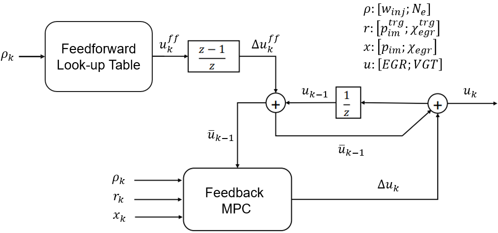
Figure 5: Schematic of look-up table FF + FB MPC architecture. Note that $\Delta u_{k}=\Delta u_{0|k}$ is computed by FB MPC, $u^{\tt ff}_{k}$ is generated by the FF look-up table, $u_{k}$ is applied to the engine, and $\bar{u}_{k-1}$ defined by (8) is provided to FB MPC.

As shown in Figure 6 for the same simple scenario as in Figure 4 and the same tuning of FB MPC, the look-up table FF was able to speed up $\chi_{\tt egr}$ tracking during fuel tip-in and tip-out and has greatly reduced the tracking error of $\chi_{\tt egr}$ during the fast ramp change of $N_{\tt e}$. For $p_{\tt im}$ tracking, the look-up table FF reduced the overshoot during the increase of $N_{\tt e}$ but it increased the tracking error during the decrease of $N_{\tt e}$. More complex simulation scenarios will be treated in Section 4.

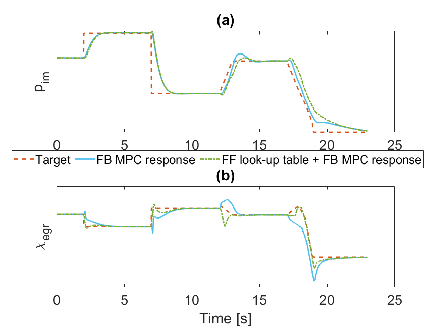
Figure 6: Example of (a) $p_{\tt im}$ and (b) $\chi_{\tt egr}$ trajectory tracking with look-up table FF and FB MPC during first, a fuel ($w_{\tt inj}$) tip-in and tip-out and then, a ramp change of $N_{\tt e}$.

We note that in the absence of the model mismatch, the conventional MPC guarantees that the true next state and predicted one-step ahead states are the same, i.e., $x_{k+1}=x_{1|k}$. This property is not maintained by the considered implementation if $u_{k}^{\tt ff}\neq u_{k-1}^{\tt ff}$. More specifically, it can be easily shown that the true state at time instant $k+1$ is given by

$$x_{k+1}=x_{1,k}+B(\rho_{k})(u_{k}^{\tt ff}-u_{k-1}^{\tt ff}),$$ (10)

$$x_{1|k}=A(\rho_{k})x_{k}+B(\rho_{k})u_{k-1}+B\Delta u_{0|k}^{*},$$ (11)

even though $u_{k}=u_{0|k}=u_{k-1}+\Delta u_{0|k}^{*}+u_{k}^{\tt ff}-u_{k-1}^{\tt ff}$. The equation (10) clarifies that the feedforward is able to affect the state of the system. From the perspective of the rate-based MPC, the term $(u_{k}^{\tt ff}-u_{k-1}^{\tt ff})$ appears as a disturbance; to accommodate it, under the assumption that $u_{k+j}^{\tt ff}=u_{k+j-1}^{\tt ff}$ over the prediction horizon (consistent with the assumption of the operating point not changing), the state constraints (5j) could be imposed on the prediction, $\bar{x}_{j|k}$, of the true state, given by

$$\bar{x}_{j|k}=x_{j|k}+\left[\sum_{m=0}^{j-1}A(\rho_{k})^{j-1-m}B(\rho_{k})\right](u_{k}^{\tt ff}-u_{k-1}^{\tt ff}).$$

This in effect tightens the constraints to accommodate changes in the feedforward. In the subsequent simulations, we did not pursue this constraint tightening approach to avoid conservatism and enforced the constraints (5j).

The solution based on look-up table FF for EGR valve and VGT positions has a drawback in that if at a given operating point $\rho_{k}$, the targets $r_{k}$ need to be different from the one assumed (e.g., EGR rate needs to be increased to satisfy different emissions regulations or during engine warm-up), the look-up table FF will no longer be accurate. The look-up table used for FF may also become inaccurate due to part-to-part variability or aging. To illustrate potential issues this may cause, Figure 7 provides simulation results for the case of constant $N_{\tt e}$ and a step-change in $w_{\tt inj}$ when the set-points for $p_{\tt im}$ and $\chi_{\tt egr}$ do not change to follow the change in $w_{\tt inj}$. The responses of the combined look-up table FF and FB MPC now exhibit large and undesirable overshoot. As this example illustrates, the mismatch of feedforwarded EGR valve and VGT positions and intake manifold pressure and EGR rate set-points can degrade the closed-loop transient response. The need to eliminate such mismatches increases calibration time and effort and can potentially necessitate a more complex implementation of the look-up table FF (e.g., multi-dimensional or adaptive look-up table). In the next section, we consider a different approach to implementing feedforward that addresses the above issue.

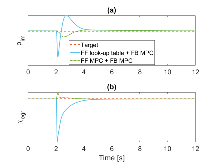
Figure 7: Example of (a) $p_{\tt im}$ and (b) $\chi_{\tt egr}$ trajectory tracking with FF look-up table and FB MPC during a step change of $w_{\tt inj}$ and constant $N_{\tt e}$. A different set of target $p_{\tt im}$ and $\chi_{egr}$ is used here without re-calibrating the FF look-up table.

3.3 Combination of FF MPC and FB MPC

The feedforward MPC (FF MPC) and FB MPC combination is illustrated in Figure 8. Unlike FB MPC, the FF MPC only closes the loop around the model of the plant, i.e., it does not use the actual engine measured signals as inputs. The primary objective of FF MPC is to approximately shape the input trajectory as needed to evolve the trajectory towards the targets.

The FF MPC is using the discrete-time model (2) for prediction. The control action is defined by solving the following discrete-time optimal control problem:

$$\min_{\tilde{u}_{0|k},...,\tilde{u}_{N-1|k}}e_{N|k}^{\sf T}P^{\tt ff}_{\infty|k}e_{N|k}+\sum_{j=0}^{N-1}e_{j|k}^{\sf T}Q^{\tt ff}e_{j|k}+\\ \tilde{u}_{j|k}^{\sf T}R^{\tt ff}\tilde{u}_{j|k}$$ (12a)

subject to

$$e_{j|k}=\tilde{x}_{j|k}-\tilde{r}_{j|k}$$ (12b)

$$\tilde{x}_{j|k}=x_{j|k}-x_{k}^{\tt ss}$$ (12c)

$$\tilde{r}_{j|k}=r_{j|k}-x_{k}^{\tt ss}$$ (12d)

$${r_{j|k}=r_{k}}$$ (12e)

$$\tilde{u}_{j|k}=u_{j|k}-u_{k}^{\tt ss}$$ (12f)

$$e_{0|k}=\tilde{x}_{k}-\tilde{r}_{k}$$ (12g)

$$e_{j+1|k}=A(\rho_{k})\tilde{x}_{j|k}+B(\rho_{k})\tilde{u}_{j|k}+e_{j|k}$$ (12h)

$$x_{\tt min}\leq x_{j|k}\leq x_{\tt max},j=1,...,N,$$ (12i)

$$u_{\tt min}\leq u_{j|k}\leq u_{\tt max},j=0,...,N-1.$$ (12j)

The final control signal is determined by (9) and (5) with $u^{\tt ff}_{k}=u^{*}_{0|k}$, where $u^{*}_{0|k}$ is the first element of the optimal solution sequence to (12).

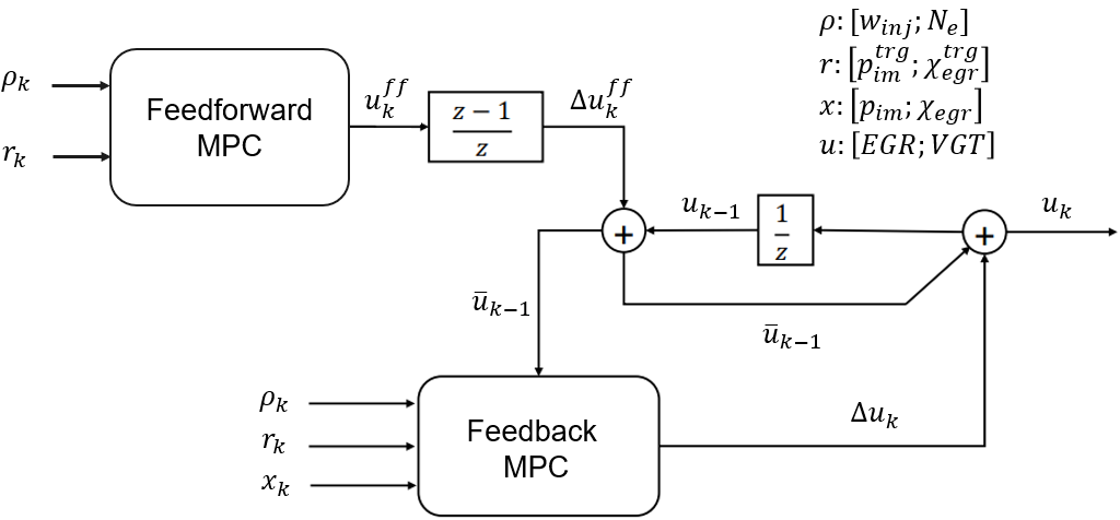
Figure 8: Schematic of FF MPC + FB MPC architecture. Note that $\Delta u$ is computed from the FB MPC, $u^{\tt ff}$ is generated by FF MPC, $u$ is applied to the engine (GT-Power model), and $\bar{u}$ is supplied to the FB controller through (8).

Simulation results of the closed-loop system with FF MPC and FB MPC combination are shown in Figure 9 for the same simple scenario as in Figure 4 and Figure 6 and same tuning of FB MPC. The responses with FF MPC match those with look-up table FF and are improved as compared to only FB MPC. More complex simulation scenarios will be treated in Section 4.

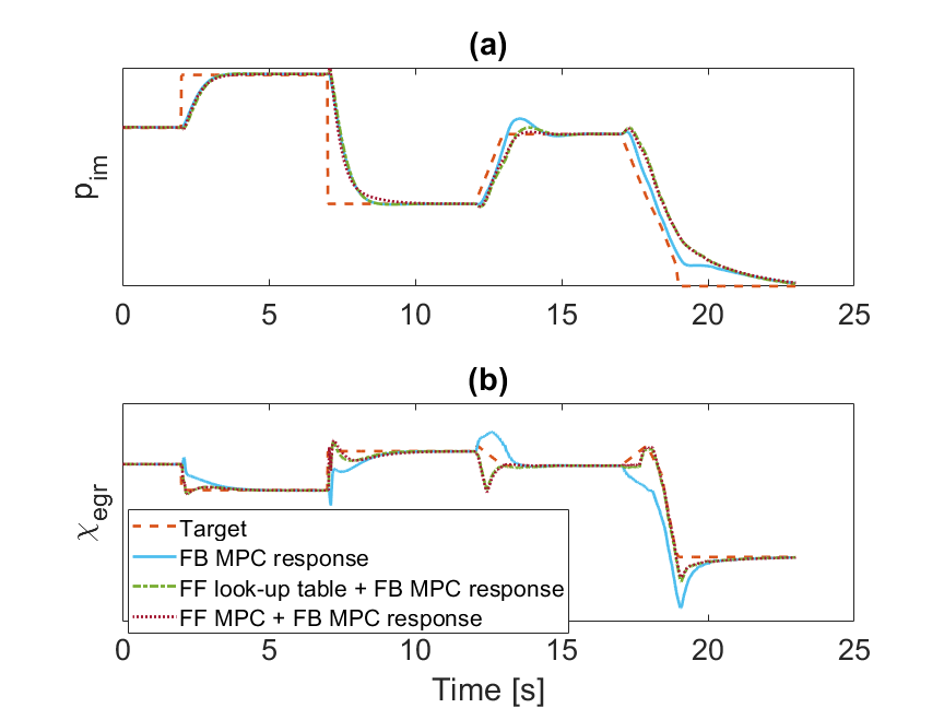
Figure 9: Example of (a) $p_{\tt im}$ and (b) $\chi_{\tt egr}$ trajectory tracking with MPC FF and FB MPC during first, a fuel ($w_{\tt inj}$) tip-in and tip-out and then, a ramp change of $N_{\tt e}$.

We note that more advanced options for integrating FF MPC and FB MPC may exist, e.g., using a sequence generated by FF MPC to warm-start FB MPC. We leave the investigation of such options to future work.

4 Simulation Results

We now evaluate the three control designs (FB MPC only, look-up table FF and FB MPC, and FF MPC and FB MPC) in more complex simulation scenarios over Federal Test Procedure (FTP) drive cycle. The results are summarized in Figures 10-11 and Table 1.In terms of average absolute tracking errors, the best tracking performance is achieved by the controller that combines FF MPC and FB MPC.

Of particular interest are large VGT excursions ending in VGT being fully open that are observed near idle with FB MPC only controller and to a lesser degree with look-up table FF and FB MPC combination. While set-point tracking is approximately maintained, these large deviations in the VGT position are indicative of potential closed-loop instability, likely caused by the state trajectory leaving the region of attraction provided by FB MPC around the current operating point $\rho_{k}$ when $\rho_{k}$ undergoes rapid transients. At the same time, FF MPC is able to to evolve the trajectory sufficiently towards new operating point to avoid instability.

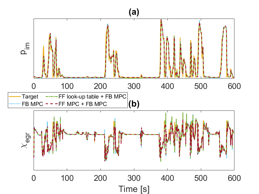
Figure 10: Time histories of (a) $p_{\tt im}$ and (b) $\chi_{\tt egr}$ with three different control schemes over the first 600 s of FTP simulation.

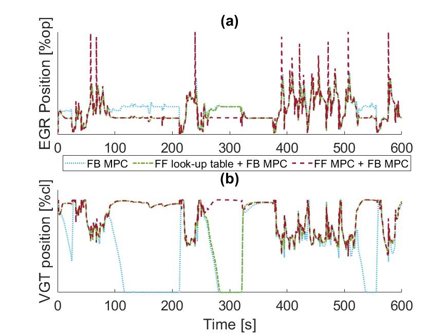
Figure 11: Time histories of (a) $EGR$ and (b) $VGT$ position with three different control schemes as in Figure 10 over the first 600 s of FTP simulation.

Table 1: Comparison of three control schemes over the FTP.

Controller	$\overline{e}_{p_{\tt im}}$[bar]	$\overline{e}_{\chi_{\tt egr}}$
FB MPC Only	0.0771	0.0144
(reference)
Look-up table FF	0.0692	0.0117
+ FB MPC	($\downarrow$ 10.3%)	($\downarrow$ 18.8%)
FF MPC	0.0650	0.0103
+ FB MPC	($\downarrow$ 15.7%)	($\downarrow$ 28.5%)

5 Conclusions

Complimenting the feedback controller based on rate-based Model Predictive Control (MPC) with the feedforward has the potential to improve the tracking performance of diesel engine airpath control systems. Such a feedforward can be based either on a look-up table or a (non-rate-based) feedforward MPC. The latter option generates dynamic feedforward trajectories and is more effective in reducing tracking errors while eliminating potential closed-loop instabilities at low engine speed by helping the state back to the region of attraction of the feedback controller.

The authors would like to acknowledge useful discussions with Dr. Dominic Liao-McPherson on the topic of diesel engine control using MPC.

References

- Bengea et al. (2004) Bengea, S., DeCarlo, R., Corless, M., and Rizzoni, G. (2004). A Polytopic system approach for the hybrid control of a diesel engine using VGT/EGR. Journal of Dynamic Systems, Measurement, and Control, 127(1), 13–21.
- Garone et al. (2011) Garone, E., Tedesco, F., and Casavola, A. (2011). Sensorless supervision of linear dynamical systems: The feed-forward command governor approach. Automatica, 47(7), 1294–1303.
- Huang et al. (2018) Huang, M., Liao-McPherson, D., Kim, S., Butts, K., and Kolmanovsky, I. (2018). Toward real-time automotive model predictive control: A perspective from a diesel air path control development. In American Control Conference. Milwaukee, WI, USA.
- Huang et al. (2016) Huang, M., Zaseck, K., Butts, K., and Kolmanovsky, I. (2016). Rate-based model predictive controller for diesel engine air path: Design and experimental evaluation. IEEE Transactions on Control Systems Technology, 24(6), 1922–1935.
- Liao-McPherson et al. (2020) Liao-McPherson, D., Huang, M., Kim, S., Shimada, M., Butts, K., and Kolmanovsky, I. (2020). Model predictive emissions control of a diesel engine airpath: Design and experimental evaluation. International Journal of Robust and Nonlinear Control, 30(17), 7446–7477.
- Liao-McPherson et al. (2017) Liao-McPherson, D., Kim, S., Butts, K., and Kolmanovsky, I. (2017). A cascaded economic model predictive control strategy for a diesel engine using a non-uniform prediction horizon discretization. In 2017 IEEE Conference on Control Technology and Applications (CCTA), 979–986. IEEE.
- Meerkov (1980) Meerkov, S. (1980). Principle of vibrational control: theory and applications. IEEE Transactions on Automatic Control, 25(4), 755–762.
- Ortner and Del Re (2007) Ortner, P. and Del Re, L. (2007). Predictive control of a diesel engine air path. IEEE transactions on control systems technology, 15(3), 449–456.
- Pannocchia et al. (2015) Pannocchia, G., Gabiccini, M., and Artoni, A. (2015). Offset-free mpc explained: novelties, subtleties, and applications. IFAC-PapersOnLine, 48(23), 342–351.
- Rawlings et al. (2017) Rawlings, J.B., Mayne, D.Q., and Diehl, M. (2017). Model predictive control: theory, computation, and design, volume 2. Nob Hill Publishing Madison, WI.
- Risbeck and Rawlings (2016) Risbeck, M. and Rawlings, J. (2016). MPCTools: Nonlinear Model Predictive Control Tools for CasADi. [online] Available: bitbucket.org/rawlings-group/octave-mpctools.
- Van Nieuwstadt et al. (2000) Van Nieuwstadt, M.J., Kolmanovsky, I.V., and Moraal, P.E. (2000). Coordinated egr-vgt control for diesel engines: an experimental comparison. SAE Transactions, 238–249.
- Wang (2004) Wang, L. (2004). A tutorial on model predictive control: Using a linear velocity-form model. Developments in Chemical Engineering and Mineral Processing, 12(5-6), 573–614.
- Zhang et al. (2022) Zhang, J., Amini, M.R., Kolmanovsky, I., Tsutsumi, M., and Nakada, H. (2022). Development of a model predictive airpath controller for a diesel engine on a high-fidelity engine model with transient thermal dynamics. In American Control Conference. Atlanta, GA, USA.