Demystifying Inferential Models: A Fiducial Perspective

Abstract

Inferential models have recently gained in popularity for valid uncertainty quantification. In this paper, we investigate inferential models by exploring relationships between inferential models, fiducial inference, and confidence curves. In short, we argue that from a certain point of view, inferential models can be viewed as fiducial distribution based confidence curves. We show that all probabilistic uncertainty quantification of inferential models is based on a collection of sets we name principle sets and principle assertions.

keywords Confidence curve, Confidence distribution, Dempster-Shafer theory, Fiducial inference, Inferential model

1 Introduction

Inferential models (IMs) (Martin and Liu, 2015b) are one of the great statistical innovations of the 2010s. IMs brought a thoroughly novel idea into the foundations of statistics by formalizing a way to assign epistemic probabilities to events that have guaranteed frequentist interpretation, called validity (Martin and Liu, 2013, 2015a, 2015c, 2015b; Martin, 2017). When studying IMs one cannot but notice that IMs share many similarities with mathematical mechanics of fiducial inference.

R.A. Fisher introduced the idea of fiducial probability (Fisher, 1930) as a potential replacement of the Bayesian posterior distribution. Although he discussed fiducial inference in several subsequent papers, there appears to be no rigorous universally accepted definition of a fiducial distribution for a vector parameter. The basic idea of the fiducial argument is switching the role of data and parameters to introduce influentially meaningful distribution on the parameter space that summarizes our knowledge about the unknown parameter without introducing any prior information.

There are various related formalization of this idea such as Dempster-Shafer (DS) theory (Dempster, 2008; Edlefsen et al., 2009; Shafer, 1976), and generalized fiducial inference (GFI) (Hannig, 2009; Hannig et al., 2016; Cui and Hannig, 2019) that has been applied to many modern statistical problems (Cisewski and Hannig, 2012; Wandler and Hannig, 2012; Lai et al., 2015; Hannig et al., 2016; Liu and Hannig, 2016, 2017; Williams and Hannig, 2019; Williams et al., 2019; Cui and Hannig, 2019; Neupert and Hannig, 2019; Cui and Hannig, 2020; Cui et al., 2021). Even objective Bayesian inference, which aims at finding non-subjective model based priors can be seen as addressing the same basic question. Examples of recent breakthroughs related to reference prior and model selection are Bayarri et al. (2012); Berger et al. (2009, 2012). There are many more references that interested readers can find in the review article Hannig et al. (2016).

Another important idea in statistical foundations that received considerable interest in the past decade is confidence distribution (CD), that some viewed as “the Neymanian interpretation of Fisher’s fiducial distributions” (Schweder and Hjort, 2016). CD refers to a data-dependent distribution function that can represent confidence intervals (regions) of all levels for a parameter of interest (Xie and Singh, 2013; Schweder and Hjort, 2016). The initial idea can be traced back to early 20th century (Neyman, 1941; Cox, 1958), but CDs have not received much attentions until the recent surge of interest in the research of CD and its applications (Efron, 1998; Schweder and Hjort, 2002, 2003, 2016; Xie et al., 2011; Singh et al., 2005, 2007; Xie and Singh, 2013; Luo et al., 2021; Lawless and Fredette, 2005; Tian et al., 2011; Yang et al., 2016; Liu et al., 2014, 2015; Cui and Xie, 2021). Heuristically speaking CD is a function of both the parameter and the sample which satisfies two conditions. The first condition basically states that for any fixed sample, a CD must be a distribution function on the parameter space. The second condition essentially places a restriction to this sample-dependent distribution function such that the corresponding inference has desired frequentist properties.

A confidence curve (CC) was introduced by Birnbaum (Birnbaum, 1961). It was originally viewed as a useful graphical tool for visualizing CDs by converting, the distribution function $H_{y}(\theta)$ to the

$$\operatorname{cc}_{y}(\theta)=2|H_{n}(\theta)-0.5|.$$ (1)

On a plot of a CC defined in (1), a line across the $y$-axis of the significance level $\alpha$, for any $0<\alpha<1$, intersects with the confidence curve at two points, that correspond to end points of the $\alpha$ level, equal tailed, two-sided confidence interval for $\theta$. In addition, the minimum of a confidence curve is the median of the CD which can serve as a point estimator. This idea has been further generalized beyond the equal-tailed univariate confidence intervals by Schweder and Hjort (Schweder and Hjort, 2016). They require that all $\{\theta:\operatorname{cc}_{y}(\theta)\leq\alpha\}$ form $\alpha$ confidence set, but these sets do not have to be intervals. The main advantage that CC has over CD is that it indicates the shape of the confidence set for each possible data $y$.

The rest of the paper is organized as follows. In Section 2, we explain mathematical definition of IMs, present a simple example, and discuss some basic properties of IMs. In Section 3, we explore relationships between GFI and IM. In particular, we investigate sets for which fiducial probability and IM belief coincide. The concept of CCs does not necessarily tell us how to obtain them. In Section 4, we show that IMs can be viewed as a tool for obtaining CCs. However they are not the only such tool, e.g., higher order likelihood inference (Fraser et al., 2009; Fraser, 2004, 2011; Fraser and Naderi, 2008; Fraser et al., 2005, 2010). Section 5 concludes by discussing our takes from the theorems proved in this paper. In particular we claim that IMs can be, in some sense, viewed as fiducial distribution based confidence curves.

While we are using GFI terminology in this paper, the same mathematical results can be formulated using the DS theory. In particular, the statements using fiducial probability can be replaced with the DS belief function, which is different from the IM belief function.

2 Inferential models revisited

There are several definitions of IMs that differ in details. In this section we present what we consider to be the most common version in the IM literature. The definition uses three steps: association, prediction and combination.

Association-step: In this step, one associates data, parameters and auxiliary random variables using a deterministic equation

$$a(Y,\theta,U)=0.$$ (2)

More precisely, this means that for all $\theta\in\Theta$ there exist random variables $U,Y$ defined on the same probability space satisfying (2), where the auxiliary variable $U$ has a known distribution $f_{U}$ free of unknown parameters, for example $U(0,1)$, and $Y$ has density $f(y|\theta)$ with respect to some dominating measure. The function $a(y,\theta,u)$ is assumed measurable. One of the consequences of the association is that for any observed $y$ there is at least one $u_{y,\theta}$ satisfying $a(y,\theta,u_{y,\theta})=0$.

Figure 1: A visualization of relationships between association, data generating and pivotal equations for a statistical model.

A well-known example of association is the pivotal equation: $T(Y,\theta)=U$, where if $Y$ follows $f(y|\theta)$ then the random variable $U$ has distribution free of unknown parameters. Another is the data generating equation (DGE) $Y=G(U,\theta)$. See Figure 1 for a visualization of relationships between association, data generating and pivotal equations.

The association is then used to obtain a collection of sets $\Theta_{y}(u)$ of candidate parameter values, where $\Theta_{y}(u)\equiv\{\theta:a(y,\theta,u)=0\}$.

Predict-step: Denote by $\theta_{0}$ the true parameter used in generating the observed data $y$. Denote by $u_{y,\theta_{0}}$ a value of $u$ that is associated by (2) with the observed data $y$ and true parameter $\theta_{0}$. The goal of this step is to predict the value of $u_{y,\theta_{0}}$. This is done using a predictive random set $\mathcal{S}:\Omega\rightarrow 2^{R(U)}$, where $R(U)$ is the range of $U$. For example, if $U$ is $U(0,1)$, then $R(U)=[0,1]$ and one possible random set is $\mathcal{S}=[0,U^{*}]$, where $U^{*}$ is another $U(0,1)$ random variable.

A good choice of $\mathcal{S}$ is crucial to the interpretation and properties of the IM. The following assumption is typically made on $\gamma(u)=P(u\in\mathcal{S})$ (Liu and Martin, 2020):

$$P(\gamma(U^{\star})\leq\alpha)\leq\alpha\mbox{ for all $\alpha\in(0,1),$}$$ (3)

where $U^{\star}$ follows the same distribution as $U$ in (2).

Combine-step: IM inference is based on a random set $\Theta_{y}(\mathcal{S})=\bigcup_{u\in\mathcal{S}}\Theta_{y}(u)$. Notice that $\Theta_{y}(\mathcal{S})$ is obtained using a process that is similar to de-pivoting in classical statistics (Casella and Berger, 2002). Evidence in favor and against any assertion $A$ is based on a relationship between the assertion $A$ and the random set $\Theta_{y}(\mathcal{S})$.

There are a number of relevant summaries of the distribution of $\theta_{y}(\mathcal{S})$. In particular, the lower probability known as belief function is defined as

$$\operatorname{bel}_{y}(A)\equiv P(\Theta_{y}(\mathcal{S})\subset A|\Theta_{y}(\mathcal{S})\neq\emptyset);$$ (4)

the upper probability known as plausibility function is defined as:

$$\operatorname{pl}_{y}(A)\equiv 1-\operatorname{bel}_{y}(A^{c})=P(\Theta_{y}(\mathcal{S})\cap A\neq\emptyset|\Theta_{y}(\mathcal{S})\neq\emptyset).$$

If the set $\{\Theta_{y}(\mathcal{S})\subset A\}$ in (4) is not measurable, regular outer measure is used.

In particular, $\operatorname{bel}_{y}(A)$ could be viewed as a measure of evidence for assertion $A$ while $1-\operatorname{pl}_{y}(A)$ as a measure of evidence against assertion $A$. The gap between $\operatorname{bel}_{y}(A)$ and $\operatorname{pl}_{y}(A)$ is an important feature of IM. However, the following proposition shows that this gap is perhaps too large.

Proposition 2.1.

If any two independent copies of the random set $\mathcal{S}$ have non-empty intersections with probability 1, then $\operatorname{bel}_{y}(A)>0$ implies $\operatorname{pl}_{y}(A)=1$.

Proof.

Consider two independent copies of the random set $\mathcal{S}_{1}$ and $\mathcal{S}_{2}$. Recall $\operatorname{bel}_{y}(A)=P(\Theta_{y}(\mathcal{S}_{1})\subset A)>0$. If $\operatorname{pl}_{y}(A)<1$, then $P(\Theta_{y}(\mathcal{S}_{2})\subset A^{\complement})>0$ which is a contradiction with the assumption $P(\mathcal{S}_{1}\cap\mathcal{S}_{2}=\emptyset)=0$. ∎

The implication of this proposition is that at most one of the probability bounds ($\operatorname{bel}_{y}(A),\operatorname{pl}_{y}(A)$) provides any useful information. Notice that any nested random set trivially satisfies the assumption of non-empty intersection.

One of the key proprieties of IMs is validity (Martin and Liu, 2015b). While the following lemma is well-known, we present its proof because it showcases an important technique used repeatedly in this manuscript.

Lemma 2.1.

Assuming (3), then for any $A$,

$$\sup_{\theta\notin A}\bar{P}_{\theta}(\operatorname{bel}_{Y}(A)\geq 1-\alpha)\leq\alpha,$$ (5)

where $\bar{P}_{\theta}$ is the regular outer measure associated with the likelihood of $Y$.

Proof.

Fix $\theta\notin A$ and because $\emptyset\subset A$ we have

$$\operatorname{bel}_{y}(A)=P(\Theta_{y}(\mathcal{S})\subset A|\Theta_{y}(\mathcal{S})\neq\emptyset)\leq P(\Theta_{y}(\mathcal{S})\subset A)\leq 1-\gamma(u_{y,\theta}),$$

where $u_{y,\theta}$ is the $u$ value associated with $y$ and $\theta$. Consequently, using the associated $Y$ and $U$

$$\bar{P}_{\theta}(\operatorname{bel}_{Y}(A)\geq 1-\alpha)\leq P(1-\gamma(U)\geq 1-\alpha)=P(\gamma(U)\leq\alpha)\leq\alpha.$$

The statement follows by taking supremum over $A^{\complement}$. ∎

Example 1.

We shall investigate IM inference for the normal location model, i.e., $Y\sim N(\theta,1)$.

$A$-step: The association between $Y$, $\theta$, and auxiliary variable $U$ can be expressed as $Y=\theta+\Phi^{-1}(U)$, where $\Phi$ is a distribution function of standard normal distribution. From here $\Theta_{y}(u)=\{y-\Phi^{-1}(u)\}$.

$P$-step: One could predict the unobserved $u$ with a predictive random set $\mathcal{S}=S_{U^{*}}$, where $U^{*}$ follows $U(0,1)$, and $S_{\alpha}$ is defined by

$$S_{\alpha}=\left\{u\in(0,1):|u-0.5|<|\alpha-0.5|\right\},\quad\alpha\in(0,1).$$ (6)

It is easy to see that $\gamma(U^{\star})\sim U(0,1)$ and (3) is satisfied.

$C$-step: Considering the choice of predictive random set $S$ in Equation (6), the random set $\Theta_{y}(\mathcal{S})$ is given by

$$\Theta_{y}(\mathcal{S})=\cup_{u\in S_{U^{*}}}\{y-\Phi^{-1}(u)\}\\ =\Big{(}y-\Phi^{-1}(0.5+|U^{*}-0.5|),y-\Phi^{-1}(0.5-|U^{*}-0.5|)\Big{)}.$$

The plausibility function is $\operatorname{pl}_{y}(\theta)=1-|2\Phi(y-\theta)-1|.$ The CC based on the usual, two sided confidence intervals (1) satisfies $\operatorname{cc}_{y}(\theta)=1-\operatorname{pl}_{y}(\theta)$. Examples of $\operatorname{cc}_{y}(\theta)$ for this problem can be found in the left two panels of Figure 2.

We end this section by stating the following important lemma.

Lemma 2.2.

Consider a random set $\mathcal{S}$ and corresponding $\gamma(u)$. The random set $\mathcal{S}^{\prime}=S_{U^{*}}$, where $U^{*}$ is $U(0,1)$ and $S_{\alpha}=\{u\,:\,\gamma(u)>1-\alpha\}$, shares the same $\gamma(u)$. Moreover, if $P(\Theta_{y}(\mathcal{S}^{\prime})\neq\emptyset)=1$, then $\operatorname{bel}_{y}(A)\leq\operatorname{bel}_{y}^{\prime}(A)$ for all $A$, where $\operatorname{bel}_{y}^{\prime}$ is the belief function associated with $\mathcal{S}^{\prime}$.

Proof.

Compute:

$$\gamma^{\prime}(u)=P(u\in\mathcal{S}^{\prime})=P\left(1-U^{*}\leq\gamma(u)\right)=\gamma(u).$$

To prove the second part of the lemma, define ${\mathcal{W}}_{y}(A)=\{u\,:\,\Theta_{y}(u)\subset A\}$. We have

$$\operatorname{bel}_{y}(A)\leq P(\mathcal{S}\subset{\mathcal{W}}_{y}(A))\leq 1-\sup\{\gamma(u):\ u\in{\mathcal{W}}_{y}(A)^{\complement}\}\\ =P(\mathcal{S}^{\prime}\subset{\mathcal{W}}_{y}(A))=\operatorname{bel}_{y}^{\prime}(A),$$

where the last equality follows because of $P(\Theta_{y}(\mathcal{S}^{\prime})\neq\emptyset)=1$. ∎

The meaning of this lemma is that in most situations only nested random sets $\mathcal{S}^{\prime}$ defined in Lemma 2.2 should be used. This is because given $\gamma(u)$ these random sets are the most efficient.

3 Generalized fiducial distribution and inferential models

Let us first quickly review the definition of generalized fiducial distribution (GFD). Interested readers can find more details in (Hannig et al., 2016). Given association (2), we define first the pseudo-solution of the association equation using the optimization problem:

$$Q_{y}(u)=\arg\min_{\theta^{\star}}{\|a(y,\theta^{\star},u)\|}.$$ (7)

Typically, $\|\cdot\|$ is either $\ell_{2}$ or $\ell_{\infty}$ norm. If there is more than one solution to (7), one minimizer is selected based on some possibly random rule. Thus when there are multiple minimizers, there are multiple versions of fiducial distribution based on which one is selected.

Next, for each small $\epsilon>0$, define the random variable $\theta_{\epsilon}^{\star}=Q_{\textbf{y}}(U_{\epsilon}^{\star})$, where $U_{\epsilon}^{\star}$ has the distribution of $U$ truncated to the set

$$\mathcal{M}_{y,\epsilon}=\{U_{\epsilon}^{\star}:\|a(y,U_{\epsilon}^{\star},\theta_{\epsilon}^{\star})\|=\|a(y,U_{\epsilon}^{\star},Q_{y}(U_{\epsilon}^{\star}))\|\leq\epsilon\},$$ (8)

i.e., having the density $f_{U}(u^{\star})I_{\mathcal{M}_{y,\epsilon}}(u^{\star})/(\int_{\mathcal{M}_{y,\epsilon}}f_{U}(u)\,du),$ where $f_{U}$ is the density of $U$. Then assuming that the random variable $\theta_{\epsilon}^{\star}$ converges in distribution as $\epsilon\to 0$, the GFD is defined as the limiting distribution of $\theta^{\star}=\lim_{\epsilon\to 0}\theta_{\epsilon}^{\star}$. The fiducial probability is then $\operatorname{fid}_{y}(A)=P(\theta^{\star}\in A)$, where the probability is based on the distribution of $\theta^{\star}$ with the observed data $y$ taken as fixed. Clearly, if $P(U^{\star}\in\mathcal{M}_{y,0})>0$ then $\theta^{\star}=\theta^{\star}_{0}$, and

$$\operatorname{fid}_{y}(A)=P(Q_{y}(U^{\star})\in A\mid U^{\star}\in\mathcal{M}_{y,0}),$$

where again $U^{\star}$ has the same distribution as $U$ in (2).

Notice that in the GFD literature the association is usually assumed to be based on a DGE. While any association equation, can be used to conduct statistical inferences, only the data generating equation is guaranteed not to lose information. This loss of information can occur when there are multiple $y$ for each $\theta$ and $u$ solving the association equation, and the inference is based on insufficient statistics.

The following theorems provide connections between IMs and GFI. They are established in terms of belief though similar statements can be derived for plausibility.

Theorem 3.1.

Consider an association (2), assume $P(U^{\star}\in\mathcal{M}_{y,0})=1$, and that the predictive random set satisfies (3). Then $\operatorname{bel}_{y}(A)\leq\operatorname{fid}_{y}(A)\leq\operatorname{pl}_{y}(A)$ for any measurable $A$.

Proof.

Define $\underline{\mathcal{U}}_{y}(A)=\{u\in\mathcal{M}_{y,0}\,:\,\Theta_{y}(u)\subset A\}=\mathcal{W}_{y}(A)\cap\mathcal{M}_{y,0}$, which is measurable because $A$ is measurable. Next, define $\overline{\mathcal{U}}_{y}(A)=\underline{\mathcal{U}}_{y}(A^{\complement})^{\complement}$. Note that because $P(U^{\star}\in\mathcal{M}_{y,0})=1$, there is no conditioning and

$$P\left(U^{\star}\in\underline{\mathcal{U}}_{y}(A)\right)\leq\operatorname{fid}_{y}(A)\leq P\left(U^{\star}\in\overline{\mathcal{U}}_{y}(A)\right).$$

Moreover, $\Theta_{y}(\mathcal{S})\subset A$ if and only if $\mathcal{S}\subset\underline{\mathcal{U}}_{y}(A)$ and therefore

$$\operatorname{bel}_{y}(A)=P(\mathcal{S}\subset\underline{\mathcal{U}}_{y}(A))\leq 1-\sup\{\gamma(u):\ u\in\underline{\mathcal{U}}_{y}(A)^{\complement}\}\equiv 1-\beta.$$

Finally, $\underline{\mathcal{U}}_{y}(A)\supset\{u:\gamma(u)>\beta\}$ and (3) imply

$$P\left(U^{\star}\in\underline{\mathcal{U}}_{y}(A)\right)\geq P(\gamma(U^{\star})>\beta)\geq 1-\beta.$$

The rest of the proof follows by the definition of $\operatorname{pl}_{y}(A)$. ∎

Theorem 3.2.

Consider association (2) with $U$ having a non-atomic distribution. For any fixed measurable set $A$ and fixed data $y$, there exists a nested random set $\mathcal{S}$ satisfying (3) and a version of fiducial distribution satisfying $\operatorname{bel}_{y}(A)=\operatorname{fid}_{y}(A)$.

Proof.

We will be using the same notation as in the proof of Theorem 3.1. If $P(U^{\star}\in\mathcal{M}_{y,0})>0$, then

$$P\left(U^{\star}\in\underline{\mathcal{U}}_{y}(A)\mid\mathcal{M}_{y,0}\right)\leq\operatorname{fid}_{y}(A)\leq P\left(U^{\star}\in\overline{\mathcal{U}}_{y}(A)\mid\mathcal{M}_{y,0}\right).$$

We can select the minimizer in (7) so that $P\left(U^{\star}\in\underline{\mathcal{U}}_{y}(A)\mid\mathcal{M}_{y,0}\right)=\operatorname{fid}_{y}(A)$. If $P(U^{\star}\in\mathcal{M}_{y,0})=0$ we can use any minimizer in (7).

Next select a collection of sets $S_{\alpha},\ \alpha\in[0,1]$ satisfying all of the following: a) $S_{\alpha}\cap\mathcal{M}_{y,0}\neq\emptyset$; b) $S_{\alpha_{1}}\subset S_{\alpha_{2}}$ whenever $\alpha_{1}<\alpha_{2}$; c) $P(U^{\star}\in S_{\alpha})=\alpha$; d) $S_{\operatorname{fid}_{y}(A)}\cap\mathcal{M}_{y,0}=\underline{\mathcal{U}}_{y}(A)$; e) $S_{\alpha}\cap\underline{\mathcal{U}}_{y}(A)^{\complement}\neq\emptyset$ whenever $\alpha>\operatorname{fid}_{y}(A)$. Such collection always exists but it is not unique. The random set $\mathcal{S}=S_{U^{*}}$, where $U^{*}$ follows $U(0,1)$, satisfies the statements of the theorem. ∎

Theorems 3.1 and 3.2 show that fiducial probability is a natural bound for IM beliefs and plausibility. This bound can be achieved for any measurable set $A$ using some random set $\mathcal{S}$. Thus one could argue that IM is less efficient than fiducial probability, i.e., the beliefs are perhaps too small and plausibilities too high. However, this gap allows IM to gain some favorable properties, such as avoiding false confidence and guaranteeing frequentist validity. However, as seen in Theorem 3.2, IM can guarantee these good properties only if the random set is selected before seeing the data. Therefore data snooping should be avoided when using IM.

Next, we show that there are many sets where belief and fiducial probabilities agree. These sets will be important in establishing a connection between IM and confidence curves.

Theorem 3.3.

Assume that the random set $\mathcal{S}$ is nested. For any data $y$ and any $\alpha\in[0,1]$, there exists a set $A_{\alpha,y}$, so that $\operatorname{bel}_{y}(A_{\alpha,y})\geq\alpha$, and $A_{\alpha,y}\subset A$ for all $A$ satisfying $\operatorname{bel}_{y}(A)\geq\alpha$, and for any $\alpha_{1}<\alpha_{2}$, we have $A_{\alpha_{1},y}\subset A_{\alpha_{2},y}$.

If additionally $P(U^{\star}\in\mathcal{M}_{y,0})=1$ and in (3) we have $\gamma(U^{\star})\sim U(0,1)$, then there is a version of $\operatorname{fid}_{y}$ satisfying $\operatorname{bel}_{y}(A_{\alpha,y})=\operatorname{fid}_{y}(A_{\alpha,y})=\alpha$ for all $\alpha$ in the range of $\operatorname{bel}_{y}$.

Proof.

Recall that the random set $\mathcal{S}$ is nested. Denote the range of the random set by $R(\mathcal{S})$ and define

$$S_{\alpha}=\bigcup_{\beta<\alpha}\bigcap\{S\in R(\mathcal{S})\,:\,P(\mathcal{S}\subset S)\geq\beta\}.$$ (9)

Because the random set is nested and by continuity of measure, $P(\mathcal{S}\subset S_{\alpha})\geq\alpha$. By definition, for any $\alpha_{1}<\alpha_{2}$ we have $S_{\alpha_{1}}\subset S_{\alpha_{2}}$.

Define $A_{\alpha,y}=\Theta_{y}(S_{\alpha})$. Clearly, $\operatorname{bel}_{y}(A_{\alpha,y})\geq\alpha$ and the sets $A_{\alpha,y}$ are nested. If $\operatorname{bel}_{y}(A)\geq\alpha$, then by definition $A_{\alpha,y}\subset A$. Moreover, if $\operatorname{bel}_{y}(A)=\alpha$ then $\operatorname{bel}_{y}(A_{\alpha,y})=\alpha$.

Under the additional assumptions and following the proof of Theorem 3.1 we have $\operatorname{fid}_{y}(A_{\alpha,y})=P(U^{\star}\in S_{\alpha})=P(\gamma(U^{\star})>1-\alpha)=\alpha.$ Here we remark that the chosen version of $\operatorname{fid}_{y}$ selects one of the minimizers in (7) that belongs to $A_{\alpha^{\prime},y}^{\complement}$ with the largest possible $\alpha^{\prime}$. ∎

Notice that Theorem 3.3 implies $\operatorname{bel}_{y}(A)=\sup\{\alpha:A_{\alpha,y}\subset A\}.$ Therefore we will call the collection of $A_{\alpha,y}$ the principle assertions of IM as they carry all the information available in the IM. In the next section we will see that principle assertions provide an important link to confidence curves. Similarly we will call $S_{\alpha}$ in (9) the principle nested sets.

4 Inferential models and confidence curves

Confidence curves could be viewed as functions whose level sets provide a collection of valid confidence intervals at all levels of confidence. The formal definition is given below:

Definition 4.1.

A function $\operatorname{cc}_{y}(\theta)\,:\mathcal{Y}\times\Theta\to[0,1]$ is a CC if for all $\alpha\in(0,1)$, $P_{\theta}(\operatorname{cc}_{Y}(\theta)<\alpha)=\alpha$. Similarly $\operatorname{cc}_{y}(\theta)$ is a conservative CC if $P_{\theta}(\operatorname{cc}_{Y}(\theta)<\alpha)\geq\alpha$, for all $\alpha\in(0,1)$.

In other words, the random confidence curve $\operatorname{cc}_{Y}(\theta)$ is uniformly distributed when $\theta$ is the true parameter. Confidence curve generalizes the idea of confidence distribution (Xie and Singh, 2013) to higher-dimensional parameters, where its contours provide a nested family of confidence regions indexed by degree of confidence (Schweder and Hjort, 2016), i.e., each $\{\theta\,:\,\operatorname{cc}_{y}(\theta)\leq\alpha\}$ is an $\alpha\cdot 100\%$ confidence set.

Example 2.

We continue Example 1. Suppose that in addition to $Y\sim N(\mu_{y},1)$ we also have $X\sim N(\mu_{x},1)$. We plot confidence curves for $\mu_{x}$ in the left panel, $\mu_{y}$ in the middle panel, and $\mu_{x}/\mu_{y}$ in the right panel of Figure 2. The confidence curve for $\mu_{x}/\mu_{y}$ is based on Fieller’s confidence set Fieller (1954). Notice that the shape of the CC indicates that based on $\alpha$ the confidence set for $\mu_{x}/\mu_{y}$ might be an interval, two disjoint intervals, or the whole real line.

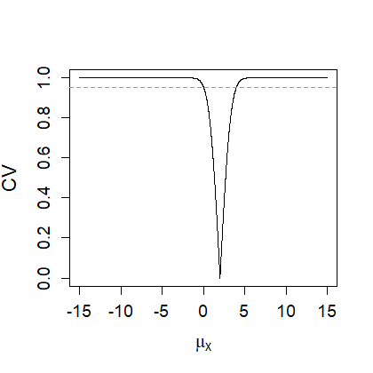
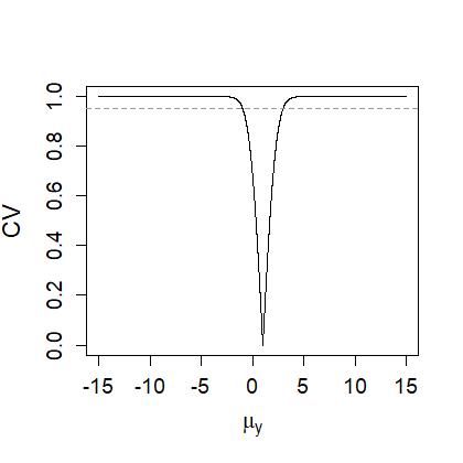
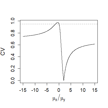
Figure 2: Confidence curves for $\mu_{x},\mu_{y},\mu_{x}/\mu_{y}$ where $X\sim N(\mu_{x},1)$, $Y\sim N(\mu_{y},1)$ given that we observe $x=2,y=1$. The dotted lines indicate 95% confidence sets.

We shall investigate the relationship of CCs to IMs next. Let us first show that CC can be used to define valid belief and plausibility functions without the use of any IM model.

Lemma 4.1.

Let $\operatorname{cc}_{y}(\theta)$ be a conservative CC. The function $\operatorname{cc-bel}_{y}(A)=\sup\{\alpha:\{\theta:\operatorname{cc}_{y}(\theta)\leq\alpha\}\subset A\}$ is a valid belief function.

Proof.

When $\operatorname{cc-bel}_{y}(A)\geq 1-\alpha$ then $\operatorname{cc}_{y}(\theta)\geq 1-\alpha$ for all $\theta\notin A$. Thus

$$P_{\theta}(\operatorname{cc-bel}_{Y}(A)\geq 1-\alpha)\leq P_{\theta}(\operatorname{cc}_{Y}(\theta)\geq 1-\alpha)=1-P_{\theta}(\operatorname{cc}_{Y}(\theta)<\alpha)\leq\alpha$$

for any $\theta\notin A$. ∎

Notice that $\operatorname{cc-pl}_{y}(A)=1-\operatorname{cc-bel}_{y}(A^{\complement})=\inf\{\operatorname{cc}_{y}(\theta):\theta\in A\}.$ Therefore $\operatorname{cc}_{y}(\theta)$ is a possibility contour in the sense of Zadeh (1978); Dubois and Prade (1988); Dubois (2006); Augustin et al. (2014). Further connections between IM and possibility theory has been explored in Liu and Martin (2020).

The previous lemma is not surprising in light of the next theorem which shows that any CC can be formally viewed as an instance of a valid IM.

Theorem 4.1.

Given a confidence curve, there exists an IM satisfying (3) which provides inference equivalent to this confidence curve.

Proof.

Denote by $\eta(u)$ the inverse of the distribution function of $\operatorname{cc}_{Y}(\theta)$. Because by definition of CC this is sub-uniform, $\eta(u)\leq u$. Thus we can consider the association:

$$a(y,\{\theta,\eta\},u)=\operatorname{cc}_{y}(\theta)-\eta(u).$$

If the CC is exact, $\eta(u)=u$, otherwise $\eta(u)\leq u$ will be viewed as an unknown parameter.

The random set is taken as $\mathcal{S}=[0,U^{*}]$, where $U^{*}\sim U(0,1)$. Note that $S_{\alpha}=[0,\alpha)$, $\gamma(u)=1-u$ and (3) is trivially satisfied.

We will use the marginal IM with

$$\Theta_{y}(S)=\{\theta:a(y,\{\theta,\eta\},u)=0,\mbox{ for some $u\in S$ and $\eta$}\}.$$

Thus $\operatorname{pl}_{y}(\{\theta\})=P(\theta\in\Theta_{y}(\mathcal{S}))=P(\operatorname{cc}_{y}(\theta)\leq U^{*})=1-\operatorname{cc}_{y}(\theta)$. Similarly, the principle assertions $A_{\alpha,Y}=\{\theta\,:\,\operatorname{cc}_{y}(\theta)\leq\alpha\}$ are exactly the same as the confidence sets implied by the CC. Consequently, $\operatorname{cc-bel}_{y}(A)=\operatorname{bel}_{y}(A)$ for all $A$. ∎

Finally, we show that any IM defines an associated CC. It also shows that fiducial probability plays a special role in this association.

Theorem 4.2.

Assume (3). The sets $A_{\alpha,y}$ defined in Theorem 3.3 are $\alpha\cdot 100\%$ confidence sets, and $\operatorname{cc}_{y}(\theta)=\inf\{\alpha\,:\,\theta\in A_{\alpha,y}\}$ is a conservative CC. Additionally, if $P(U^{\star}\in\mathcal{M}_{y,0})=1$ then the actual coverage of $A_{\alpha,y}$ is given by $\operatorname{fid}_{y}(A_{\alpha,y})$, where we use the version of $\operatorname{fid}_{y}$ introduced in the proof of Theorem 3.3. Consequently, $\operatorname{cc}_{y}^{\prime}(\theta)=\inf\{\operatorname{fid}_{y}(A_{\alpha,y})\,:\,\theta\in A_{\alpha,y}\}\geq\operatorname{cc}_{y}(\theta)$ is an exact CC.

Proof.

We will be using the notation introduced in Section 3. Let $\theta$ and $U$ be the parameter and ancillary random variable associated with data $Y$ by (2). Then, just as in the proof of Theorem 3.1,

$$P_{\theta}(\theta\in A_{\alpha,Y})=P(U\in S_{\alpha})\geq P(\gamma(U)>1-\alpha)\geq\alpha.$$ (10)

Additionally, if $P(U^{\star}\in\mathcal{M}_{y,0})=1$ then $\operatorname{fid}_{y}(A_{\alpha,y})=P(U^{\star}\in S_{\alpha})$, which does not depend on $y$, and as seen in the first equality in (10) is the coverage of $A_{\alpha,y}$.

The statements about CCs follow by definition. ∎

5 Discussion

The results in Section 4 show that the key concept of validity is innate to CCs. In other words, IMs are valid when they produce valid CCs. However, the property of CC does not come with a recipe on how to produce it. The big advantage of IMs is that its three-step recipe provides a systematic way to produce CCs.

As seen in Theorem 4.2 principle assertions $A_{\alpha,y}$ provide the main link between IM and CC. It may be of interest to point out that $A_{\alpha,y}$ is a confidence set that is obtained by de-pivoting of the principle nested set $S_{\alpha}$ using the association (2). Moreover, its coverage is given by the fiducial probability $\operatorname{fid}_{y}(A)$.

In other words, IM answers an old question, when are (fiducial) credible intervals confidence intervals, i.e., what sets of fiducial probability $\alpha$ are $\alpha\cdot 100\%$ confidence sets? The answer given in Theorem 3.2 is that technically it could be any measurable set as long as for all the unobserved data $y^{\prime}$ we would use the corresponding principle assertion $A_{\alpha,y^{\prime}}$ de-pivoted from the principle nested set $S_{\alpha}$ from the proof of Theorem 3.2. This is of course unrealistic and only set $A_{\alpha,y}$ obtained by de-pivoting a sensible $S_{\alpha}$ chosen prior to seeing the data will be a set of fiducial probability $\alpha$ that is also $\alpha\cdot 100\%$ confidence sets.

While most of the results linking GFD and IM are proved under the assumption $P(U^{\star}\in\mathcal{M}_{y,0})=1$, the same results remain true if conditioning on $\{U^{\star}\in\mathcal{M}_{y,0}\}$ is effectively conditioning on ancillary statistic (Martin and Liu, 2015a), e.g., maximal invariant sigma algebra of a group model. If the conditioning in GFD is not conditioning on ancillary statistic, the relationship between IM and GFD is complicated and needs to be studied further.

In conclusion, IM can be viewed as fiducial distribution based confidence curves. They provide a powerful argument for anyone seeking fiducial or objective Bayes distributions on parameter space to consider making calculations on the auxiliary $U$ and pay attention to how are the credible sets linked across all potential unobserved data $y^{\prime}$.

6 Acknowledgements

Jan Hannig’s research was supported in part by the National Science Foundation under Grant No. DMS-1916115 and 2113404.

References

- Augustin et al. (2014) Augustin, T., Coolen, F. P., De Cooman, G., and Troffaes, M. C. (2014), Introduction to imprecise probabilities, John Wiley & Sons.
- Bayarri et al. (2012) Bayarri, M. J., Berger, J. O., Forte, A., and García-Donato, G. (2012), “Criteria for Bayesian model choice with application to variable selection,” The Annals of Statistics, 40, 1550–1577.
- Berger et al. (2009) Berger, J. O., Bernardo, J. M., and Sun, D. (2009), “The formal definition of reference priors,” The Annals of Statistics, 37, 905–938.
- Berger et al. (2012) — (2012), “Objective priors for discrete parameter spaces,” Journal of the American Statistical Association, 107, 636–648.
- Birnbaum (1961) Birnbaum, A. (1961), “Confidence Curves: An Omnibus Technique for Estimation and Testing Statistical Hypotheses,” Journal of the American Satistical Association, 56, 246–249.
- Casella and Berger (2002) Casella, G. and Berger, R. L. (2002), Statistical inference, Pacific Grove, CA: Wadsworth and Brooks/Cole Advanced Books and Software, 2nd ed.
- Cisewski and Hannig (2012) Cisewski, J. and Hannig, J. (2012), “Generalized Fiducial Inference for Normal Linear Mixed Models,” The Annals of Statistics, 40, 2102–2127.
- Cox (1958) Cox, D. R. (1958), “Some Problems Connected with Statistical Inference,” Ann. Math. Statist., 29, 357–372.
- Cui and Hannig (2019) Cui, Y. and Hannig, J. (2019), “Nonparametric generalized fiducial inference for survival functions under censoring (with discussions and rejoinder),” Biometrika, 106, 501–518.
- Cui and Hannig (2020) — (2020), “A fiducial approach to nonparametric deconvolution problem: discrete case,” arXiv preprint arXiv:2006.05381.
- Cui et al. (2021) Cui, Y., Hannig, J., and Kosorok, M. (2021), “A unified nonparametric fiducial approach to interval-censored data,” arXiv preprint arXiv:2111.14061.
- Cui and Xie (2021) Cui, Y. and Xie, M.-g. (2021), “Confidence Distribution and Distribution Estimation for Modern Statistical Inference,” arXiv preprint arXiv:2109.01898.
- Dempster (2008) Dempster, A. P. (2008), “The Dempster-Shafer Calculus for Statisticians,” International Journal of Approximate Reasoning, 48, 365–377.
- Dubois (2006) Dubois, D. (2006), “Possibility theory and statistical reasoning,” Computational statistics & data analysis, 51, 47–69.
- Dubois and Prade (1988) Dubois, D. and Prade, H. (1988), Possibility theory: an approach to computerized processing of uncertainty, Plenum Press, New York.
- Edlefsen et al. (2009) Edlefsen, P. T., Liu, C., and Dempster, A. P. (2009), “Estimating limits from Poisson counting data using Dempster–Shafer analysis,” The Annals of Applied Statistics, 3, 764–790.
- Efron (1998) Efron, B. (1998), “R.A.Fisher in the 21st Century,” Statistical Science, 13, 95–122.
- Fieller (1954) Fieller, E. C. (1954), “Some problems in interval estimation,” Journal of the Royal Statistical Society: Series B (Methodological), 16, 175–185.
- Fisher (1930) Fisher, R. A. (1930), “Inverse probability,” Proceedings of the Cambridge Philosophical Society, xxvi, 528–535.
- Fraser et al. (2009) Fraser, A. M., Fraser, D. A. S., and Staicu, A.-M. (2009), “The second order ancillary: A differential view with continuity,” Bernoulli. Official Journal of the Bernoulli Society for Mathematical Statistics and Probability, 16, 1208–1223.
- Fraser and Naderi (2008) Fraser, D. and Naderi, A. (2008), “Exponential models: Approximations for probabilities,” Biometrika, 94, 1–9.
- Fraser et al. (2005) Fraser, D., Reid, N., and Wong, A. (2005), “What a model with data says about theta,” International Journal of Statistical Science, 3, 163–178.
- Fraser (2004) Fraser, D. A. S. (2004), “Ancillaries and Conditional Inference,” Statistical Science, 19, 333–369.
- Fraser (2011) — (2011), “Is Bayes posterior just quick and dirty confidence?” Statistical Science, 26, 299–316.
- Fraser et al. (2010) Fraser, D. A. S., Reid, N., Marras, E., and Yi, G. Y. (2010), “Default Priors for Bayesian and frequentist inference,” Journal of the Royal Statistical Society, Series B, 72.
- Hannig (2009) Hannig, J. (2009), “On Generalized Fiducial Inference,” Statistica Sinica, 19, 491–544.
- Hannig et al. (2016) Hannig, J., Iyer, H., Lai, R. C., and Lee, T. C. (2016), “Generalized Fiducial Inference: A Review and New Results,” Journal of the American Statistical Association, 111, 1346–1361.
- Lai et al. (2015) Lai, R. C. S., Hannig, J., and Lee, T. C. M. (2015), “Generalized Fiducial Inference for Ultrahigh-Dimensional Regression,” Journal of the American Statistical Association, 110, 760–772.
- Lawless and Fredette (2005) Lawless, J. F. and Fredette, M. (2005), “Frequentist prediction intervals and predictive distributions,” Biometrika, 92, 529–542.
- Liu and Martin (2020) Liu, C. and Martin, R. (2020), “Inferential models and possibility measures,” arXiv preprint arXiv:2008.06874.
- Liu et al. (2014) Liu, D., Liu, R., and Xie, M. (2014), “Exact Meta-Analysis Approach for Discrete Data and its Application to 2 x 2 Tables With Rare Events,” Journal of the American Statistical Association, 109.
- Liu et al. (2015) Liu, D., Liu, R. Y., and Xie, M. (2015), “Multivariate Meta-Analysis of Heterogeneous Studies Using Only Summary Statistics: Efficiency and Robustness.” Journal of the American Statistical Association, 110 509, 326–340.
- Liu and Hannig (2016) Liu, Y. and Hannig, J. (2016), “Generalized fiducial inference for binary logistic item response models,” Psychometrika, 81, 290–324.
- Liu and Hannig (2017) — (2017), “Generalized Fiducial Inference for Logistic Graded Response Models,” Psychometrika, 82, 1097–1125.
- Luo et al. (2021) Luo, X., Dasgupta, T., Xie, M., and Liu, R. Y. (2021), “Leveraging the Fisher randomization test using confidence distributions: Inference, combination and fusion learning,” Journal of the Royal Statistical Society: Series B (Statistical Methodology), 83, 777–797.
- Martin (2017) Martin, R. (2017), Inferential Models, American Cancer Society, pp. 1–8.
- Martin and Liu (2013) Martin, R. and Liu, C. (2013), “Inferential models: A framework for prior-free posterior probabilistic inference,” Journal of the American Statistical Association, 108, 301 – 313.
- Martin and Liu (2015a) — (2015a), “Conditional inferential models: combining information for prior-free probabilistic inference,” Journal of the Royal Statistical Society, Series B, 77, 195–217.
- Martin and Liu (2015b) — (2015b), Inferential Models: Reasoning with Uncertainty, Chapman & Hall/CRC Monographs on Statistics & Applied Probability, CRC Press.
- Martin and Liu (2015c) — (2015c), “Marginal inferential models: prior-free probabilistic inference on interest parameters,” Journal of the American Statistical Association, 110, 1621–1631.
- Neupert and Hannig (2019) Neupert, S. D. and Hannig, J. (2019), “BFF: Bayesian, Fiducial, Frequentist Analysis of Age Effects in Daily Diary Data,” The Journals of Gerontology: Series B, gbz100.
- Neyman (1941) Neyman, J. (1941), “Fiducial Argument and the Theory of Confidence Intervals,” Biometrika, 32, 128–150.
- Schweder and Hjort (2003) Schweder, T. and Hjort, N. (2003), “Frequentist analogues of priors and posteriors,” Econometrics and The Philosophy of Economics, 285–317.
- Schweder and Hjort (2002) Schweder, T. and Hjort, N. L. (2002), “Confidence and likelihood,” Scandinavian Journal of Statistics, 29, 309–332.
- Schweder and Hjort (2016) — (2016), Confidence, likelihood, probability, vol. 41, Cambridge University Press.
- Shafer (1976) Shafer, G. (1976), A mathematical theory of evidence, Princeton university press Princeton.
- Singh et al. (2005) Singh, K., Xie, M., and Strawderman, W. E. (2005), “Combining information from independent sources through confidence distributions,” The Annals of Statistics, 33, 159–183.
- Singh et al. (2007) — (2007), “Confidence Distribution (CD): Distribution Estimator of a Parameter,” Lecture Notes-Monograph Series, 54, 132–150.
- Tian et al. (2011) Tian, L., Wang, R., Cai, T., and Wei, L.-J. (2011), “The Highest Confidence Density Region and Its Usage for Joint Inferences about Constrained Parameters,” Biometrics, 67, 604–10.
- Wandler and Hannig (2012) Wandler, D. V. and Hannig, J. (2012), “Generalized fiducial confidence intervals for extremes,” Extremes, 15, 67–87.
- Williams and Hannig (2019) Williams, J. P. and Hannig, J. (2019), “Nonpenalized variable selection in high-dimensional linear model settings via generalized fiducial inference,” Ann. Statist., 47, 1723–1753.
- Williams et al. (2019) Williams, J. P., Storlie, C. B., Therneau, T. M., Jr, C. R. J., and Hannig, J. (2019), “A Bayesian Approach to Multistate Hidden Markov Models: Application to Dementia Progression,” Journal of the American Statistical Association, 0, 1–21.
- Xie and Singh (2013) Xie, M. and Singh, K. (2013), “Confidence Distribution, the Frequentist Distribution Estimator of a Parameter: A Review,” International Statistical Review, 81, 3 – 39.
- Xie et al. (2011) Xie, M., Singh, K., and Strawderman, W. E. (2011), “Confidence distributions and a unified framework for meta-analysis,” Journal of the American Statistical Association, 106, 320–333.
- Yang et al. (2016) Yang, G., Liu, D., Wang, J., and Xie, M.-g. (2016), “Meta-analysis framework for exact inferences with application to the analysis of rare events,” Biometrics, 72, 1378–1386.
- Zadeh (1978) Zadeh, L. A. (1978), “Fuzzy sets as a basis for a theory of possibility,” Fuzzy sets and systems, 1, 3–28.