The Fluctuating Two-Ray Fading Model with Independent Specular Components

Abstract

We introduce and characterize the independent fluctuating two-ray (IFTR) fading model, a class of fading models consisting of two specular components which fluctuate independently, plus a diffuse component modeled as a complex Gaussian random variable. The IFTR model complements the popular fluctuating two-ray (FTR) model, on which the specular components are fully correlated and fluctuate jointly. The chief probability functions of the received SNR in IFTR fading, including the PDF, CDF and MGF, are expressed in closed-form, having a functional form similar to other state-of-the-art fading models. Then, the IFTR model is empirically validated using multiple channels measured in rather diverse scenarios, including line of sight (LOS) millimeter-wave, land mobile satellite (LMS) and underwater acoustic communication (UAC), showing a better fit than the original FTR model and other models previously used in these environments. Additionally, the performance of wireless communication systems operating under IFTR fading is evaluated in closed-form in two scenarios: (i) exact and asymptotic bit error rate for a family of coherent modulations; and (ii) exact and asymptotic outage probability.

I Introduction

Small-scale fading is a key propagation effect in many wireless scenarios. The accurate modeling of this phenomenon in the millimeter-wave (mmWave) band has become particularly relevant because of its use in the fifth generation (5G) standard. This also applies to land mobile satellite (LMS) channels, which are attracting an increasing interest as the sixth generation (6G) standard is expected to integrate space-ground links to provide global coverage [1]. This propagation phenomenon also occurs even in environments where information is conveyed by means of non-electromagnetic waves, as in underwater acoustic communications (UAC) [2].

The Rice distribution has been largely employed to model line of sight (LOS) wireless channels. Recent attempts to characterize fading in mmWave channels, for instance, have used it [3, 4]. Two refinements of the Ricie model are of particular interest because of their relevant physical interpretation: one considers that the LOS (or specular) component considered in the Rice model fluctuates randomly. This yields the Rician-shadowed distribution, which has been employed to model LMS channels [5]. The second one considers an additional specular component, yielding the two-wave with diffuse power (TWDP) model [6, 7], which has proven to outperform the Rice distribution when modeling indoor channels at 60 GHz [8].

The fluctuating two-ray (FTR) model was recently proposed as a natural generalization of both the Rician-shadowed and the TWDP models, and many others [9]. It consists of two specular components with random phases that jointly fluctuate, plus a diffuse component. The FTR model not only provides a better fit to mmWave field measurements than previous fading models, but also its primary probability functions - CDF, probability density function (PDF) and moment generating function (MGF) - can be expressed in closed-form.

However, the physical model that originates FTR fading assumes that the two specular components experience a common (i.e., fully correlated) fluctuation, which may not always be the case in practice. For instance, the specular components may fluctuate because of two different phenomena as they reach the destination through different paths, thus being affected by different scatterers and/or perturbations. As we will later see, this situation is quite common in practice. Besides capturing the reality of a number of propagation mechanisms, allowing the specular components to fluctuate independently provides an additional degree of freedom that results in an improved modeling of these scenarios, which can be quite significant in some cases. For instance, in terms of the CDF, this is translated into an increased flexibility to change its log-log concavity and convexity, yielding a better fit to experimental data.

A special case of this scenario was originally suggested in [9], where the two specular components undergo independent and identically distributed (iid) Nakagami-$m$ fluctuations. However, a thorough statistical characterization and analysis was not presented, and has never been carried out in the literature to the best of our knowledge. In this paper, we introduce, characterize and validate the independent fluctuating two-ray (IFTR) fading model to complement the FTR model by allowing the specular components to fluctuate independently and experience dissimilar fading severity, i.e., the specular components fluctuate according to non-necessarily identical distributions. Specifically, the following key contributions are made in this context:

• Closed-form expressions for the PDF, CDF, and MGF of the received power envelope, or equivalently the signal-to-noise ratio (SNR), under IFTR fading are obtained.

• It is shown that the IFTR model fits measured channels in rather diverse scenarios such as mmWave, LMS and UAC better than the FTR model and other state-of-the-art models previously used in these environments.

• The performance of communication systems operating in these propagation conditions is analyzed, in terms of the exact and asymptotic bit error rate (BER) for a family of modulations, and in terms of the outage probability.

• The influence of the model parameters on the fading statistics and on the system performance is investigated, and the key differences with respect to the FTR model are assessed.

The remainder of this paper is organized as follows. Section II presents the physical channel model for the IFTR fading. Its statistical characterization in terms of the MGF, PDF, and CDF of the received SNR is carried out in Section III. Section IV shows the empirical validation of the newly proposed IFTR fading model. Based on the obtained statistical functions, performance analysis of wireless communications systems undergoing IFTR fading is exemplified in Section V. Numerical results are given in Section VI, and the main conclusions are summarized in Section VII.

II Channel model

Let us assume that the small-scale fluctuations in the amplitude of a signal transmitted over a wireless channel are given by two fluctuating dominant waves, referred to as specular components, to which other diffusely propagating waves are added. The complex baseband voltage of the wireless channel of this model can be expressed as

$$\begin{split}V_{r}=\sqrt{\zeta_{1}}V_{1}\exp\left({j\phi_{1}}\right)+\sqrt{\zeta_{2}}V_{2}\exp\left({j\phi_{2}}\right)+X+jY,\end{split}$$ (1)

where $\sqrt{\zeta_{i}}V_{i}\exp\left({j\phi_{i}}\right)$ represents the i-th specular component $(i=1,2)$, which is assumed to have an average amplitude $V_{i}$ modulated by a random variable $\sqrt{\zeta_{i}}$ responsible for its fluctuation, where $\zeta_{1}$ and $\zeta_{2}$ are independent unit-mean Gamma distributed random variables with PDF

$$f_{\zeta_{i}}\left(u\right)=\frac{m_{i}^{m_{i}}u^{m_{i}-1}}{\Gamma\left({m_{i}}\right)}e^{-m_{i}u},\quad\quad i=1,2.$$ (2)

Without any loss of generality, in the sequel we will assume $V_{1}\geq V_{2}$. The i-th specular component is assumed to have a uniformly distributed random phase $\phi_{i}$, such that $\phi_{i}\sim\mathcal{U}[0,2\pi)$, with $\phi_{1}$ and $\phi_{2}$ considered to be statistically independent. On the other hand, $X+jY$ is a complex Gaussian random variable, such that $X,Y\sim\mathcal{N}(0,\sigma^{2})$, representing the diffuse received signal component due to the combined reception of numerous weak, independently-phased scattered waves. This model will be referred to as the IFTR fading model. Note that if $m_{1},m_{2}\rightarrow\infty$ then $\zeta_{1},\zeta_{2}\rightarrow 1$, i.e., the fluctuation of the specular components tends to disappear and the IFTR model tends to the TWDP fading model proposed by Durgin, Rappaport and De Wolf [6], also known as the Generalized Two-Ray fading model with Uniformly distributed phases (GTR-U) [7].

As with the TWDP fading model, the IFTR channel model can conveniently be described in terms of the parameters $K$ and $\Delta$, defined as

$$K\triangleq\frac{V_{1}^{2}+V_{2}^{2}}{2\sigma^{2}},$$ (3)

$$\Delta\triangleq\frac{2V_{1}V_{2}}{V_{1}^{2}+V_{2}^{2}},$$ (4)

where the parameter $K$ represents the ratio of the average power of the dominant (specular) components to the power of the remaining diffuse multipath. On the other hand, $\Delta$ is a parameter ranging from 0 to 1 capturing how similar to each other are the average received powers of the specular components: when the average magnitudes of the two specular components are equal, we have $\Delta=1$. Conversely, in the absence of a second component ($V_{1}=0$ or $V_{2}=0$), then $\Delta=0$. The IFTR model is an alternative generalization of the TWDP model, which differs from the original FTR model proposed by the authors in [9]. The IFTR model can be applied in those situations in which the specular components follow very different paths and are affected by different scatterers.

III Statistical characterization

We will first characterize the distribution of the received power envelope associated with the IFTR fading model, or equivalently, the distribution of the received SNR. After passing through the multipath fading channel, the signal will be affected by additive white Gaussian noise (AWGN) with one-sided power spectral density $N_{0}$. The statistical characterization of the instantaneous SNR, here denoted as $\gamma$, is crucial for the analysis and design of wireless communications systems, as many performance metrics in wireless communications are a function of the SNR.

The received average SNR $\bar{\gamma}$ after transmitting a symbol with energy density $E_{s}$ undergoing a multipath fading channel as described in (1) will be

$$\begin{split}&\bar{\gamma}=\left({E_{s}/N_{0}}\right){\mathbb{E}}\left\{{\left|{V_{r}}\right|^{2}}\right\}=\left({E_{s}/N_{0}}\right)\left({V_{1}^{2}+V_{2}^{2}+2\sigma^{2}}\right)\cr&\quad\quad=\left({E_{s}/N_{0}}\right)2\sigma^{2}\left({1+K}\right),\cr\end{split}$$ (5)

where $\mathbb{E}\{\cdot\}$ denotes the expectation operator.

With all the above definitions, the chief probability functions related to the FTR fading model can now be computed.

III-A MGF

In the following lemma we show that, for the IFTR fading model, it is possible to obtain the MGF of $\gamma$ in closed-form.

Lemma 1

Let us consider the IFTR fading model as described in (1)-(2). Then, the MGF of the received SNR $\gamma$ will be given by (6), where ${}_{2}F_{1}(\cdot)$ is the Gauss hypergeometric function [10, p. 556 (15.1.1)].

$$\begin{split}&M_{\gamma}\left(s\right)={{1+K}\over{1+K-\bar{\gamma}s}}{{m_{1}^{m_{1}}}\over{\left[{m_{1}-{K\over 2}\left({1+\sqrt{1-\Delta^{2}}}\right){{\bar{\gamma}s}\over{1+K-\bar{\gamma}s}}}\right]^{m_{1}}}}{{m_{2}^{m_{2}}}\over{\left[{m_{2}-{K\over 2}\left({1-\sqrt{1-\Delta^{2}}}\right){{\bar{\gamma}s}\over{1+K-\bar{\gamma}s}}}\right]^{m_{2}}}}\cr&\quad\quad\times\,_{2}F_{1}\left({m_{1},m_{2};1;{{K^{2}\Delta^{2}}\over{\left[{2m_{1}{{1+K-\bar{\gamma}s}\over{\bar{\gamma}s}}-K\left({1+\sqrt{1-\Delta^{2}}}\right)}\right]\left[{2m_{2}{{1+K-\bar{\gamma}s}\over{\bar{\gamma}s}}-K\left({1-\sqrt{1-\Delta^{2}}}\right)}\right]}}}\right).\cr\end{split}$$ (6)

Proof:

See Appendix A. ∎

When any of the parameters $m_{1}$ or $m_{2}$ takes an integer value, the MGF of the SNR in the IFTR fading model can be calculated as a finite sum of elementary functions.

Corollary 1

When $m_{1}\in\mathbb{Z}^{+}$, the MGF of the SNR $\gamma$ of the IFTR fading channel can be expressed as a finite sum of elementary terms as given in (7).

$$\begin{split}&M_{\gamma}\left(s\right)=\frac{{1+K}}{{1+K-\bar{\gamma}s}}m_{1}^{m_{1}}m_{2}^{m_{2}}\left[{m_{1}-\frac{K}{2}\left({1+\sqrt{1-\Delta^{2}}}\right)\frac{{\bar{\gamma}s}}{{1+K-\bar{\gamma}s}}}\right]^{m_{2}-m_{1}}\sum\limits_{n=0}^{m_{1}-1}{\frac{1}{{n!}}\binom{m_{1}-1}{n}}\frac{{\Gamma\left({m_{2}+n}\right)}}{{\Gamma\left({m_{2}}\right)}}\cr&\quad\times\left({\frac{{K\Delta}}{2}\frac{{\bar{\gamma}s}}{{1+K-\bar{\gamma}s}}}\right)^{2n}\left[{m_{1}m_{2}-\left({m_{1}\frac{K}{2}\left({1-\sqrt{1-\Delta^{2}}}\right)+m_{2}\frac{K}{2}\left({1+\sqrt{1-\Delta^{2}}}\right)}\right)\frac{{\bar{\gamma}s}}{{1+K-\bar{\gamma}s}}}\right]^{-m_{2}-n}.\cr\end{split}$$ (7)

Proof:

See Appendix B. ∎

Remark 1

For the case when $m_{2}\in\mathbb{Z}^{+}$ and $m_{1}$ is not necessarily an integer, the MGF of $\gamma$ can be calculated by using (7) and interchanging $m_{1}$ and $m_{2}$ and also interchanging the occurences of ${+\sqrt{1-\Delta^{2}}}$ and ${-\sqrt{1-\Delta^{2}}}$. In the sequel, the interchanging of these parameters will also hold in the subsequent expressions obtained for $m_{1}\in\mathbb{Z}^{+}$, when the case $m_{2}\in\mathbb{Z}^{+}$ wants to be considered instead.

III-B PDF and CDF

We now show that the PDF and CDF of the IFTR distribution can also be obtained in closed-form, provided that any of the parameters $m_{1}$ or $m_{2}$ is restricted to take a positive integer value. We note that the general case of arbitrary real $m_{1}$ and $m_{2}$ can always be numerically computed by an inverse Laplace transform over the MGF.

We derive closed-form expressions for the PDF and CDF of the SNR (or, equivalently, the power envelope) for the IFTR fading model, which will be demonstrated in the next lemma.

Lemma 2

When $m_{1}\in\mathbb{Z}^{+}$, the PDF and CDF of the SNR $\gamma$ in a FTR fading channel can be expressed in terms of the confluent hypergeometric function $\Phi_{2}(\cdot)$ defined in [11, p. 34, (8)], as given, respectively, in (8) and (9).

$$\begin{split}&f_{\gamma}(x)=\frac{{1+K}}{{\bar{\gamma}}}m_{1}^{m_{1}}m_{2}^{m_{2}}\left({m_{1}+\frac{K}{2}\left({1+\sqrt{1-\Delta^{2}}}\right)}\right)^{m_{2}-m_{1}}\sum\limits_{n=0}^{m_{1}-1}{\frac{1}{{n!}}\binom{m_{1}-1}{n}}\frac{{\Gamma\left({m_{2}+n}\right)}}{{\Gamma\left({m_{2}}\right)}}\left({\frac{{K\Delta}}{2}}\right)^{2n}\cr&\quad\quad\times\left[{m_{1}\frac{K}{2}\left({1-\sqrt{1-\Delta^{2}}}\right)+m_{2}\frac{K}{2}\left({1+\sqrt{1-\Delta^{2}}}\right)+m_{1}m_{2}}\right]^{-m_{2}-n}\cr&\quad\quad\times\;\Phi_{2}^{(3)}\left({n+1-m_{1},m_{1}-m_{2},m_{2}+n;1;-\frac{{1+K}}{{\bar{\gamma}}}x,-\frac{{m_{1}(1+K)}}{{\left(m_{1}+\frac{K}{2}\left({1+\sqrt{1-\Delta^{2}}}\right)\right)\bar{\gamma}}}x,}\right.\cr&\quad\quad\quad\quad\quad\quad\quad\quad\quad\quad\quad\quad\quad\quad\quad\quad\left.{-\frac{{m_{1}m_{2}(1+K)}}{{\left(m_{1}\frac{K}{2}\left({1-\sqrt{1-\Delta^{2}}}\right)+m_{2}\frac{K}{2}\left({1+\sqrt{1-\Delta^{2}}}\right)+m_{1}m_{2}\right)\bar{\gamma}}}x}\right).\cr\end{split}$$ (8)

$$\begin{split}&F_{\gamma}(x)=\frac{{1+K}}{{\bar{\gamma}}}m_{1}^{m_{1}}m_{2}^{m_{2}}\left({m_{1}+\frac{K}{2}\left({1+\sqrt{1-\Delta^{2}}}\right)}\right)^{m_{2}-m_{1}}\sum\limits_{n=0}^{m_{1}-1}{\frac{1}{{n!}}\binom{m_{1}-1}{n}}\frac{{\Gamma\left({m_{2}+n}\right)}}{{\Gamma\left({m_{2}}\right)}}\left({\frac{{K\Delta}}{2}}\right)^{2n}\cr&\quad\quad\times\left[{m_{1}\frac{K}{2}\left({1-\sqrt{1-\Delta^{2}}}\right)+m_{2}\frac{K}{2}\left({1+\sqrt{1-\Delta^{2}}}\right)+m_{1}m_{2}}\right]^{-m_{2}-n}\cr&\quad\quad\times\;x\Phi_{2}^{(3)}\left({n+1-m_{1},m_{1}-m_{2},m_{2}+n;2;-\frac{{1+K}}{{\bar{\gamma}}}x,-\frac{{m_{1}(1+K)}}{{\left(m_{1}+\frac{K}{2}\left({1+\sqrt{1-\Delta^{2}}}\right)\right)\bar{\gamma}}}x,}\right.\cr&\quad\quad\quad\quad\quad\quad\quad\quad\quad\quad\quad\quad\quad\quad\quad\quad\left.{-\frac{{m_{1}m_{2}(1+K)}}{{\left(m_{1}\frac{K}{2}\left({1-\sqrt{1-\Delta^{2}}}\right)+m_{2}\frac{K}{2}\left({1+\sqrt{1-\Delta^{2}}}\right)+m_{1}m_{2}\right)\bar{\gamma}}}x}\right).\cr\end{split}$$ (9)

Proof:

See Appendix C. ∎

Note that despite requiring the evaluation of a confluent hypergeometric function, the PDF and CDF of the IFTR fading model can be expressed in terms of a well-known function in communication theory. In fact, the $\Phi_{2}(\cdot)$ function also makes appearances in the CDF of common fading models such as Rician-shadowed or $\kappa$-$\mu$ shadowed [12, 13]. Moreover, this function can be efficiently evaluated using a numerical inverse Laplace transform [14]. Thus, the evaluation of the IFTR distribution functions does not pose any additional challenge compared to other state-of-the-art fading models, including the FTR fading model.

Also note that the PDF and CDF of the received signal envelope, $r=\left|V_{r}\right|$, can be easily derived from (8) and (9) by a simple change of variables. Specifically, we can write $f_{r}(r)=2rf_{\gamma}(r^{2})$ and $F_{r}(r)=F_{\gamma}(r^{2})$, with $\bar{\gamma}$ in (8) and (9) replaced by $\Omega=\mathbb{E}\{r^{2}\}$. In order to illustrate the influence of the independent fluctuation of the specular components on the fading statistics, the PDF of the received signal envelope $r$ of the IFTR and FTR models are compared for the same level of fluctuation, $m=m_{1}=m_{2}$. Results for $m=2$ and $m=10$ are shown in Fig. 1. As expected, differences between both PDFs are larger for low values of $m$ and $(m_{1},m_{2})$, which correspond to larger fluctuations in the specular components, i.e., larger fading severity. As $m,m_{1},m_{2}\rightarrow\infty$, the fluctuation decreases and both models tend to the TWDP model.

The asymmetric fluctuation of the specular components gives the IFTR model a remarkable flexibility to change the shape of the PDF. This is shown in Fig. 2, where the PDF of the SNR is depicted for different values of $m_{1}$ and $m_{2}$ when $\Delta=0.9$ and $\Delta=0.1$. In all cases $K=15$ and $\bar{\gamma}=1$. For reference, it is also represented the PDF of the Rician-shadowed model with $m=3$ [5]. It can be seen that, when $\Delta=0.1$, one of the specular components dominates ($V_{1}\gg V_{2}$) and the PDF of the IFTR distribution tends to that of the Rician-shadowed model with $m=m_{1}$. When $\Delta=0.9$, both specular components have similar amplitudes and the differences with the Rician-shadowed distribution are noticeable.

The independent fluctuation of the specular components results in an increased ability of the CDF to modify its log-log convexity and concavity, even when $m_{1}=m_{2}$. This can be observed in Fig. 3, where the CDF of the SNR for different values of the IFTR parameters are shown. The probability of severe fading is higher for $\Delta=0.9$ because the amplitude of the specular components is similar, and therefore destructive multipath combination occurs more likely. The probability of the specular components to cancel each other is also higher for low values of $m_{1}$ and $m_{2}$, i.e., when the fluctuations are larger. In these circumstances, the influence of $K$ is small, since the modulus of the sum $\sqrt{\zeta_{1}}V_{1}\exp\left({j\phi_{1}}\right)+\sqrt{\zeta_{2}}V_{2}\exp\left({j\phi_{2}}\right)$ in (1) will be generally small with respect to the power of the diffuse term, irrespectively of the magnitude of $V_{1}^{2}+V_{2}^{2}$. Conversely, deep-fading probability reduces as $\Delta$ decreases, because one of the specular components becomes much larger than the other.

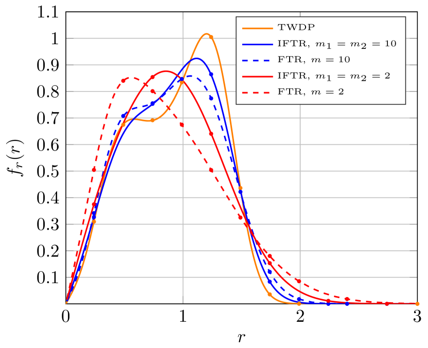
Figure 1: PDF of the received signal envelope under FTR and IFTR fading for $K=15$, $\Delta=0.9$, $\Omega=1$ and different values of $m=m_{1}=m_{2}$. Markers correspond to simulation results.

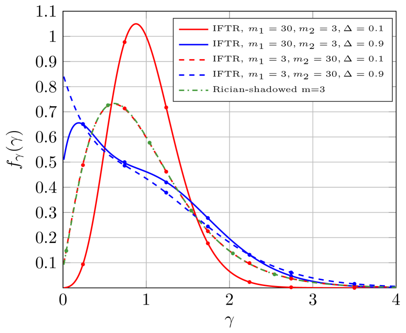
Figure 2: PDF of the SNR under Rician-shadowed and IFTR fading with $\bar{\gamma}=1,K=15$ and different values of $m_{1}$, $m_{2}$ and $\Delta$. Markers correspond to simulation results.

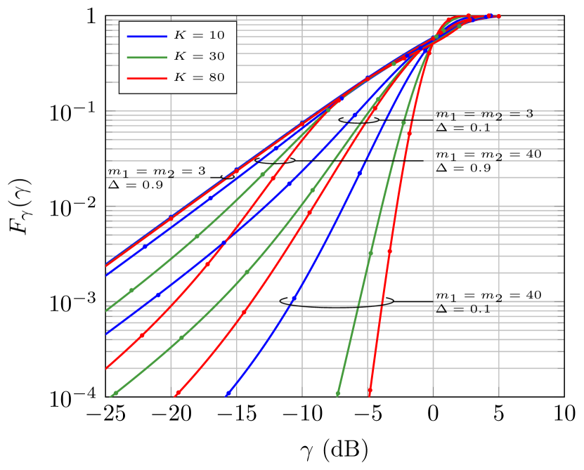
Figure 3: CDF of the SNR under IFTR fading for $\bar{\gamma}=1$ and different values of the model parameters. Markers correspond simulation results.

IV Empirical validation

This section illustrates the capability of the IFTR fading to model the small-scale fading in quite diverse scenarios. Three types of outdoor communication links are considered: the LOS mmWave channels given in [3] and [4], the LMS channels in [5] and the UAC channels measured in [15, 2]. It will be shown that the IFTR model provides a better fit to the experimental datasets than the models previously used in each of these scenarios, and also than the FTR model.

The goodness of fit between the analytical CDF of the considered model, $F_{a}(x)$, and the empirical one estimated from measurements, $F_{e}(x)$, is quantified by using the following modified version of the Kolmogorov-Smirnov (KS) statistic:

$$\epsilon=\max_{x}\left|\log_{10}F_{e}(x)-\log_{10}F_{a}(x)\right|.$$ (10)

The logarithm in (10) is used to magnify the errors between the CDFs in the region close to zero. The rationale to overweight these values is that some of the key performance metrics of communication systems, e.g., the BER and the outage probability, are determined by the probability of deep fading events. Hence, improving the goodness of the fitting in this region is more important.

The number of parameters of the IFTR distribution to be optimized depends on the considered experimental dataset. In the mmWave and UAC channels, the empirical CDF of $x=r^{2}/\mathbb{E}\{r^{2}\}$ is given [3, 4, 15, 2], while the one of $x=r^{2}$ is reported in [5]. Hence, in addition to $m_{1},m_{2},K$ and $\Delta$, the optimum value of $\Omega=\mathbb{E}\{r^{2}\}$ has to be determined also in the latter. Similar considerations apply to the remaining models included in the analysis.

IV-A mmWave channels

Two outdoor LOS radio channels are considered in this subsection: a cross-polarized channel measured at 28 GHz, from now on referred to as Ch. 1, and a co-polarized one measured at 73 GHz, referred to as Ch. 2. The empirical CDFs of their small-scale fading amplitudes are given in [3, Fig. 6] and [4, Fig. 3], respectively. The capability of the IFTR fading to model these channels is compared to that of the Rice distribution, which has been previously used to model LOS channels in these bands. Moreover, the TWDP fading is also considered for completeness, since the analysis in [8] supports that it is favored over the Rice one. As both the IFTR and the FTR models generalize the TWDP one, the comparison is useful to assess the potential gain given by the fluctuations in the specular components in terms of fitting quality.

Table I shows the fitting error and the optimum model parameters for the aforementioned channels. For the case of Ch. 1 the IFTR fading model yields a lower error than the FTR one, which already improves the results achieved by the TWDP fading model. We see that the Rice model provides the largest error. In Ch. 2 the improvement of the IFTR model with respect to the remaining models is even higher, and is actually quite significant. Interestingly, the TWDP and the FTR models achieve the same error as with the Rice model only in their limiting cases, i.e., $\Delta=0$ in the TWDP model and ($\Delta=0,m\rightarrow\infty$) in the FTR one. This might erroneously lead to conclude that the second specular component and the LOS fluctuation are superfluous to model this channel. However, the results achieved by the IFTR fading model suggest otherwise, indicating that the consideration of both components is beneficial as long as their fluctuation level can be independently controlled. Hence, the large value of $m_{1}$ suggests that the specular component with larger amplitude experiences almost no fluctuation, i.e., $\zeta_{1}$ is almost constant, while the lower amplitude component $\sqrt{\zeta_{2}}V_{2}$ fluctuates considerably.

TABLE I: Fitting results for the mmWave channels

		Model
Channel	Param.	IFTR	FTR	TWDP	Rice
Ch. 1	$\epsilon$	0.2203	0.2246	0.2267	0.3298
	$K$	476.1454	80.3916	23.1347	3.5820
	$\Delta$	0.8463	0.5873	0.8619	-
	$\left(m_{1},m_{2}\right)/m$	(9, 50.5)	2	-	-
Ch. 2	$\epsilon$	0.2068	0.3228	0.3228	0.3228
	$K$	154.3797	45.4773	45.4773	45.4773
	$\Delta$	0.2170	0.0000	0.0000	-
	$\left(m_{1},m_{2}\right)/m$	(60, 3.6)	$\infty$	-	-

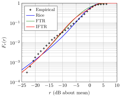
Figure 4: Empirical and theoretical CDFs of the received signal amplitude for mmWave Ch. 1 [9, Fig. 8].

The enhanced modeling capacity of the IFTR model can be graphically interpreted in terms of its flexibility to modify the concavity and convexity of the CDF (in a log-log scale). We illustrate this fact by reproducing the empirical and theoretical CDFs of the Rice and FTR models for Ch. 1 given in [9, Fig. 8], along with the CDF of the IFTR model. Results are shown in Fig. 4, where it can be seen that the CDF of the IFTR model is convex for $0<r<5$ dB, concave for $r$ around $-5$ dB, and convex again for $r<-17.5$ dB.

IV-B LMS channels

The small-scale fading in LMS channels has been widely modeled using the Rician-shadowed distribution, where the LOS component is assumed to undergo Nakagami-$m$ fading. The IFTR model can be seen as a generalization of the Rician-shadowed one. The capability of the IFTR fading to outperform the Rician-shadowed fading model is assessed by using the channels in [5, Fig. 1], where the empirical CDFs of two channels at 870 MHz are provided: one experiencing light shadowing, and another one affected by heavy shadowing caused by a denser tree cover.

Table II shows the fitting results for the IFTR, FTR and Rician-shadowed models. For the sake of fairness, the parameters of the latter (denoted using the subscript RS) have been computed to minimize the error in (10), as the ones provided in [5] were obtained with a different metric. It can be seen that the IFTR model yields better fitting results than the other models for both channels. In the light shadowing channel, the high value of $m_{\rm RS}$ suggests that the LOS term is essentially constant. Moreover, the FTR model achieves the error of the Rician-shadowed one only in its limiting case, $\Delta=0$ and $m\rightarrow\infty$. These facts might again lead to conclude that a single specular component with constant amplitude suffices to adequately model this channel. In fact, the Rice distribution with $K=3.1075$ yields the same error as these two models (although not explicitly shown in Table II). However, the values ($m_{1}=14,m_{2}=0.8)$ of the IFTR model indicate that two specular components, with considerable fluctuation in the one with lower amplitude, may be more adequate for a proper channel modeling.

The improved capability of the IFTR distribution to model the two considered channels can be graphically observed in Fig. 5, where the empirical and theoretical complementary s of the received signal envelope are shown. For coherence, axes have been scaled as in [5, Fig. 1]. Hence, errors have to be measured as the horizontal distance between the empirical and theoretical (logarithm of the) CCDF for a given value of the received signal level. In the heavily-shadowed channel, where all models fit the CCDF almost equally well in the low signal level region, the flexibility of the IFTR model is clearly noticeable in the high signal level region, where its CCDF changes from (log-log) convex to concave as the received signal level decreases. In the light-shadowing channel, the lower error of the IFTR model is due to its ability to achieve a better trade-off than the remaining models between the fitting in the low signal level region, where errors are overweighted, and in the high signal level zone, where they have been considered less relevant.

TABLE II: Fitting results for the LMS channels

		Model
Channel	Parameter	IFTR	FTR	Rician shadowed
Light shad.	$\epsilon$	0.0442	0.0507	0.0507
	$K$	479.8224	4.0542	-
	$\Delta/b_{0_{\rm RS}}$	0.8290	0	0.2025
	$\Omega/\Omega_{\rm RS}$	1.6692	1.6896	1.2847
	$\left(m_{1},m_{2}\right)/m/m_{\rm RS}$	(14, 0.8)	$\infty$	100
Heavy shad.	$\epsilon$	0.0655	0.0672	0.0673
	$K$	2.7457	0.7484	-
	$\Delta/b_{0_{\rm RS}}$	0.9997	0.6040	0.0429
	$\Omega/\Omega_{\rm RS}$	0.1289	0.1121	0.0258
	$\left(m_{1},m_{2}\right)/m/m_{\rm RS}$	(2, 0.1)	2	100

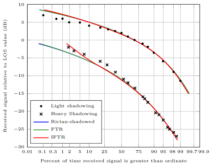
Figure 5: Empirical and theoretical CCDFs of the received signal amplitude for the light and heavy shadowing LMS channels given in [5, Fig. 1].

IV-C UAC channels

UAC channels in shallow waters exhibit multipath propagation and fading. The former is due to the reflections in the seabed, the surface of the sea and other objects, while the latter is caused by the surface waves (which change the reflection angles), internal waves and the motion of the communication ends, among other factors [16].

The $\kappa$-$\mu$ shadowed distribution, which generalizes the Rice and Rician-shadowed ones, has been proposed to model these effects [2]. However, $\mu\in\mathbb{R}$ values are employed to this end. This considerably hinders the physical interpretation of the model (which requires $\mu\in\mathbb{Z}^{+}$ according to the physical model definition in [13]), and the generation of random variables for simulation purposes [17, 13]. Hence, it is of practical interest to assess its fitting capabilities also when constraining $\mu\in\mathbb{Z}^{+}$. It must be recalled that, for practical purposes, the IFTR model employed in this section is also constrained to have $m_{1}\in\mathbb{Z}^{+}$, to allow for the analytical calculation of the PDF, despite random variables following the IFTR distribution can be easily generated according to (1) for non-negative real values of $m_{1}$. The same applies to the FTR model, where $m\in\mathbb{Z}^{+}$ is also considered.

The ability of the IFTR model to fit UAC channels is assessed by using the measurements in [15, 2]. They provide a characterization of 10 channels corresponding to links with lengths 50, 100 and 200 m, measured in Mediterranean shallow waters with a sandy seabed and depths from 14 to 30 m, approximately. The transmitter and receiver where placed at depths 3, 6 and 9 m. Sounding signals of 32, 64 and 128 kHz were transmitted. For coherence with [15, 2], channels are denoted using the nomenclature [A$|$B$|$C]D-F, where the A$|$B$|$C denotes the link length (50$|$100$|$200 m, respectively), D indicates the transmitter-receiver depth in meters and F the frequency of the transmitted signal in kHz.

The IFTR model fits these 10 channels better than the $\kappa-\mu$ shadowed model with $\mu\in\mathbb{Z}^{+}$, except for the case of C9-32, where it yields the same error. For conciseness, only the results obtained in one channel of each length (50, 100 and 200 m) are shown in Table III, where the values corresponding to the FTR model are also shown. As in the previous scenarios, the flexibility of the IFTR fading model to control the fluctuations in each specular component independently is also exploited in this context. In channels A6-32 and B6-64 the specular component with lower amplitude is almost constant, and the component with larger amplitude exhibits considerable fluctuations. In channel C3-64, the fluctuation of the specular component with larger amplitude is much lower than the one with lower amplitude, but still considerable.

As illustrated in the previous scenarios, the independent fluctuation of the specular components results in an increased ability of the CDF to change from concave to convex, and vice-versa. This can be observed in Fig. 6, where the empirical and theoretical CDFs corresponding to channel B6-64 are shown. It can be seen that the CDF of the IFTR distribution is (log-log) concave around $r=5$ dB, convex around $r=0$ dB, and concave again for $r<-5$ dB.

TABLE III: Fitting results for the UAC channels

		Model
Channel	Parameter	IFTR	FTR	$\kappa-\mu$ shadowed
A6-32	$\epsilon$	0.0569	0.0622	0.0682
	$K/\kappa$	466.2619	4.8472	1.9494
	$\Delta/\mu$	0.8720	0.9510	1
	$\left(m_{1},m_{2}\right)/m/m_{\kappa-\mu}$	(2, 60)	24	1.3088
B6-64	$\epsilon$	0.0746	0.0886	0.0758
	$K/\kappa$	508.9355	499942.1713	51.3649
	$\Delta/\mu$	0.9598	0.5256	1
	$\left(m_{1},m_{2}\right)/m/m_{\kappa-\mu}$	(4, 60)	1	0.9360
C3-64	$\epsilon$	0.1880	0.1969	0.1979
	$K/\kappa$	501.1807	5.4941	6.3239
	$\Delta/\mu$	0.5662	0	1
	$\left(m_{1},m_{2}\right)/m/m_{\kappa-\mu}$	(7, 0.75)	$\infty$	24.2813

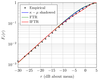
Figure 6: Empirical and theoretical CDFs of the received signal amplitude for the B6-64 UAC channel given in [15, 2].

V Performance analysis of wireless communications systems

After providing a thorough empirical validation of the IFTR fading model in a number of scenarios, it is time to illustrate how the exact closed-form expressions of the statistics of the SNR can be used for performance analysis. For exemplary purposes, we calculate the BER for a family of coherent modulations, and the outage probability.

V-A Average BER

The conditional error probability (CEP), i.e., the error rate under additive white Gaussian noise (AWGN), for many wireless communication systems with coherent detection is determined by [18]

$$P_{E}\left(\gamma\right)=\sum\limits_{r=1}^{R}{\alpha_{r}Q\left({\sqrt{\beta_{r}\gamma}}\right)},$$ (11)

where $Q(\cdot)$ is the Gauss $Q$-function and $\left\{{\alpha_{r},\beta_{r}}\right\}_{r=1}^{R}$ are modulation-dependent constants.

The average error rates for the CEP given in (11) can be calculated in terms of the CDF of the SNR as [9]

$$\overline{P_{e}}=\sum\limits_{r=1}^{R}\alpha_{r}\int^{\infty}_{0}{\sqrt{\frac{{\beta_{r}}}{{8\pi x}}}}e^{-\frac{{\beta_{r}x}}{2}}F_{\gamma}(x)dx.$$ (12)

Introducing (9) into (12), and with the help of [11, p. 286, (43)], a compact exact expression of the average BER can be found, as given in (13), in terms of the Lauricella function $F_{D}(\cdot)$ defined in [11, p. 33, (4)].

$$\begin{split}&\overline{P_{e}}=\frac{{1+K}}{{\bar{\gamma}}}m_{1}^{m_{1}}m_{2}^{m_{2}}\left({m_{1}+\frac{K}{2}\left({1+\sqrt{1-\Delta^{2}}}\right)}\right)^{m_{2}-m_{1}}\sum\limits_{n=0}^{m_{1}-1}{\frac{1}{{n!}}\binom{m_{1}-1}{n}}\frac{{\Gamma\left({m_{2}+n}\right)}}{{\Gamma\left({m_{2}}\right)}}\left({\frac{{K\Delta}}{2}}\right)^{2n}\cr&\quad\quad\times\left[{m_{1}\frac{K}{2}\left({1-\sqrt{1-\Delta^{2}}}\right)+m_{2}\frac{K}{2}\left({1+\sqrt{1-\Delta^{2}}}\right)+m_{1}m_{2}}\right]^{-m_{2}-n}\sum\limits_{r=1}^{R}{\alpha_{r}\frac{1}{{2\beta_{r}}}}\cr&\quad\quad\times\;F_{D}^{(3)}\left({\frac{3}{2},n+1-m_{1},m_{1}-m_{2},m_{2}+n;2;-\frac{{2(1+K)}}{{\beta_{r}\bar{\gamma}}},-\frac{{2m_{1}(1+K)}}{{\beta_{r}\left({m_{1}+\frac{K}{2}\left({1+\sqrt{1-\Delta^{2}}}\right)}\right)\bar{\gamma}}},}\right.\cr&\quad\quad\quad\quad\quad\quad\quad\quad\quad\quad\quad\quad\quad\quad\quad\quad\quad\quad\left.{-\frac{{2m_{1}m_{2}(1+K)}}{{\beta_{r}\left({m_{1}\frac{K}{2}\left({1-\sqrt{1-\Delta^{2}}}\right)+m_{2}\frac{K}{2}\left({1+\sqrt{1-\Delta^{2}}}\right)+m_{1}m_{2}}\right)\bar{\gamma}}}}\right).\cr\end{split}$$ (13)

Although the derived BER expression can be easily computed using the Euler form of the $F_{D}$ function, it does not provide insight about the impact of the different system parameters on performance. We now present an asymptotic, yet accurate, simple expression for the error rate in the high SNR regime. First, note that the equality in (14) holds for the asymptotic behavior of the MGF, where we write a function $a(x)$ as $o(x)$ if $\lim_{x\rightarrow\infty}a(x)/x=0$. Thus, performing a similar approach to that in [19, Propositions 1 and 3], and after some algebraic manipulation, the asymptotic BER expression given in (15) is obtained.

$$\begin{split}&\left|{M_{\gamma}\left(s\right)}\right|=\frac{{1+K}}{{\bar{\gamma}\left|s\right|}}\frac{{m_{1}^{m_{1}}}}{{\left[{m_{1}+\frac{K}{2}\left({1+\sqrt{1-\Delta^{2}}}\right)}\right]^{m_{1}}}}\frac{{m_{2}^{m_{2}}}}{{\left[{m_{2}+\frac{K}{2}\left({1-\sqrt{1-\Delta^{2}}}\right)}\right]^{m_{2}}}}\cr&\quad\quad\times\,_{2}F_{1}\left({m_{1},m_{2};1;\frac{{K^{2}\Delta^{2}}}{{\left[{2m_{1}+K\left({1+\sqrt{1-\Delta^{2}}}\right)}\right]\left[{2m_{2}+K\left({1-\sqrt{1-\Delta^{2}}}\right)}\right]}}}\right)+o\left({\left|s\right|^{-1}}\right).\cr\end{split}$$ (14)

$$\begin{split}&\overline{P_{e}}\approx\frac{{1+K}}{{2\bar{\gamma}}}\frac{{m_{1}^{m_{1}}}}{{\left[{m_{1}+\frac{K}{2}\left({1+\sqrt{1-\Delta^{2}}}\right)}\right]^{m_{1}}}}\frac{{m_{2}^{m_{2}}}}{{\left[{m_{2}+\frac{K}{2}\left({1-\sqrt{1-\Delta^{2}}}\right)}\right]^{m_{2}}}}\left({\sum\limits_{r=1}^{R}{\frac{{\alpha_{r}}}{{\beta_{r}}}}}\right)\cr&\quad\quad\times\,_{2}F_{1}\left({m_{1},m_{2};1;\frac{{K^{2}\Delta^{2}}}{{\left[{2m_{1}+K\left({1+\sqrt{1-\Delta^{2}}}\right)}\right]\left[{2m_{2}+K\left({1-\sqrt{1-\Delta^{2}}}\right)}\right]}}}\right),\quad\bar{\gamma}\gg 1.\cr\end{split}$$ (15)

V-B Outage probability

The instantaneous channel capacity per unit bandwidth is well-known to be given by

$$C=\log_{2}(1+\gamma).$$ (16)

We define the outage capacity probability, or simply outage probability, as the probability that the instantaneous channel capacity $C$ falls below a predefined threshold $R_{S}$ (given in terms of rate per unit bandwidth), i.e.,

$$P_{\rm out}=P\left({C<R_{S}}\right)=P\left({\log_{2}(1+\gamma)<R_{S}}\right).$$ (17)

Therefore

$$P_{\rm out}=P\left({\gamma<2^{R_{S}}-1}\right)=F_{\gamma}\left({2^{R_{S}}-1}\right).$$ (18)

Thus, the outage probability can be directly calculated from (9) specialized for $x=2^{R_{S}}-1$. This expression is exact and holds for all SNR values; however, it offers little insight about the effect of parameters on system performance. Fortunately, we can obtain a simple expression in the high SNR regime as follows: From (9) and [19, Proposition 5], the CDF of $\gamma$ can be written as given in (19). Therefore, the outage probability can be approximated in the large SNR regime by introducing (19) into (18).

$$\begin{split}&F_{\gamma}(x)=\frac{{1+K}}{{\bar{\gamma}}}\frac{{m_{1}^{m_{1}}}}{{\left[{m_{1}+\frac{K}{2}\left({1+\sqrt{1-\Delta^{2}}}\right)}\right]^{m_{1}}}}\frac{{m_{2}^{m_{2}}}}{{\left[{m_{2}+\frac{K}{2}\left({1-\sqrt{1-\Delta^{2}}}\right)}\right]^{m_{2}}}}\cr&\quad\quad\quad\times\,_{2}F_{1}\left({m_{1},m_{2};1;\frac{{K^{2}\Delta^{2}}}{{\left[{2m_{1}+K\left({1+\sqrt{1-\Delta^{2}}}\right)}\right]\left[{2m_{2}+K\left({1-\sqrt{1-\Delta^{2}}}\right)}\right]}}}\right)x+o\left({\bar{\gamma}^{-1}}\right).\cr\end{split}$$ (19)

VI Numerical results

In this section, numerical results are presented to evaluate the performance metrics of point-to-point wireless systems undergoing IFTR fading. Monte-Carlo simulations are used in all instances to validate the obtained closed-form expressions.

Figs. 7 shows the BER of the BPSK modulation versus the average SNR. Results obtained with the closed-form exact and asymptotic BER expressions given in (13) and (15) (with $R=1$, $\alpha_{1}=1$ and $\beta_{1}=2$), respectively, are given for $K=15$, $\Delta=0.5$, $m_{2}=2$ and different values of $m_{1}$. BER values obtained under FTR fading with the same $K,\Delta$ and $m=m_{1}$ are also given as a reference, to better highlight the differences between both models. It can be seen that there is a rather good match between the asymptotic and the exact BER in the high SNR region, and performance increases when $m_{1}$ raises due to lower fading severity. Similarly, differences between the IFTR and the FTR models also increase with $m_{1}$, being about 3.6 dB for $m_{1}=m=40$. The worse (higher) BER of the IFTR fading in this case is due to the large fluctuation experienced by the specular component with amplitude $V_{2}$, which in the FTR fading is almost negligible as $m=40$.

Fig. 8 shows the outage probability versus the average SNR for $R_{s}=2$. Results are plotted for $\Delta=0.1$ and $\Delta=0.9$ and various combinations of $m_{1},m_{2}$ and $K$. It can be seen that the outage probability decreases as $\Delta$ becomes lower, since in that case one specular component is much larger than the other one and it is unlikely that they cancel out each other. In these circumstances, performance also improves as $m_{1}$ increases, because the fluctuation of the largest specular component becomes smaller. It can also be noticed that the influence of $K$ is higher for $\Delta=0.1$, where cancellation of the specular components is unlikely.

For $\bar{\gamma}>5$ (dB), the outage probability decreases as $K$ increases, except for $(m_{1}=2,m_{2}=8)$ and $\Delta=0.9$, where performance is lower for $K=80$ than for $K=10$. This occurs because having a destructive combination of the specular components becomes more detrimental as $K$ increases, since almost all the received signal power is conveyed by the specular components as $K\to\infty$. When $\Delta<1$, the probability of destructive sum depends on the specific fluctuation of the specular components, and becomes larger as the fluctuation of the larger specular component increases, i.e., $m_{1}$ decreases. This is reflected by the fact that the outage probability is higher for $(m_{1}=2,m_{2}=8)$ than for $(m_{1}=8,m_{2}=2)$. The asymmetry in the fluctuation of the specular components becomes immaterial when $\Delta=1$, where $(m_{1}=2,m_{2}=8)$ and $(m_{1}=8,m_{2}=2)$ yielding the same outage probabilities (not explicitly shown in Fig. 8).

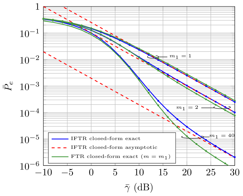
Figure 7: Exact and asymptotic closed-form BER vs. average SNR for BPSK modulation under IFTR and FTR fading with $K=15$, $\Delta=0.5$, $m_{2}=2$ and different values of $m_{1}=m$. Markers denote results obtained using Monte-Carlo simulations.

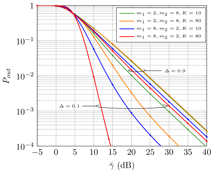
Figure 8: Outage probability vs. average SNR for $R_{s}=2$ and different combinations of $m_{,}1,m_{2},K$ and $\Delta$. Markers denote results obtained using Monte-Carlo simulations.

VII Conclusion

In this work, a new small-scale fading model consisting of two specular components with independent fluctuation plus a diffuse term has been introduced for the first time in the literature. The IFTR fading model innovates over the FTR model, whose specular components jointly fluctuate, and generalizes previous models such as the Rice, Rician-Shadowed, TWDP and others. The IFTR model has a clear physical interpretation, as it models the case where the specular waves follow very different paths and are affected by different scatterers and/or perturbations. The presented results suggest that this situation is quite common in rather diverse scenarios such as LOS mmWave, LMS and UAC channels.

Closed-form expressions for the PDF, CDF and MGF of the received SNR, expressed in terms of functions used in other state-of-the-art fading models, have been provided and double-checked. The IFTR model is shown to fit channels measured in a number of scenarios better than the FTR model and other previously proposed models. The outage probability and the error performance of wireless communication systems over channels with IFTR fading have been obtained in closed-form.

Appendix A Proof of Lemma 1

Let us consider the fading channel model given in (1) conditioned to a particular realization $\zeta_{1}=u_{1}$, $\zeta_{2}=u_{2}$ of the random variables modeling the fluctuation of the specular components. In this case, we can write

$$\left.{V_{r}}\right|_{u_{1},u_{2}}=\sqrt{u}_{1}V_{1}\exp\left({j\phi_{1}}\right)+\sqrt{u}_{2}V_{2}\exp\left({j\phi_{2}}\right)+X+jY.$$ (20)

This corresponds to the classical TWDP fading model where the amplitudes of the specular components are given by $\sqrt{u}_{1}V_{1}$ and $\sqrt{u}_{2}V_{2}$, for which the following ancillary parameters can be defined:

$$K_{u_{1},u_{2}}={{u_{1}V_{1}^{2}+u_{2}V_{2}^{2}}\over{2\sigma^{2}}},$$ (21)

$$\Delta_{u_{1},u_{2}}={{2\sqrt{u_{1}u_{2}}V_{1}V_{2}}\over{u_{1}V_{1}^{2}+u_{2}V_{2}^{2}}}.$$ (22)

The conditional average SNR for the fading model described in (20) will be

$$\begin{split}&\bar{\gamma}_{u_{1},u_{2}}=\left({E_{s}/N_{0}}\right)\left({u_{1}V_{1}^{2}+u_{2}V_{2}^{2}+2\sigma^{2}}\right)\cr&\quad\quad=\left({E_{s}/N_{0}}\right)2\sigma^{2}\left({1+K_{u_{1},u_{2}}}\right).\cr\end{split}$$ (23)

The MGF of the TWDP fading model was shown in [7] to be given in closed-form as

$$\begin{split}\quad M_{\gamma_{{}_{u_{1},u_{2}}}}\left(s\right)&={{1+K_{u_{1},u_{2}}}\over{1+K_{u_{1},u_{2}}-\bar{\gamma}_{{}_{u_{1},u_{2}}}s}}\cr&\times\exp\left({{{K_{u_{1},u_{2}}\bar{\gamma}_{u_{1},u_{2}}s}\over{1+K_{u_{1},u_{2}}-\bar{\gamma}_{u_{1},u_{2}}s}}}\right)\cr&\times I_{0}\left({{{\Delta_{u_{1},u_{2}}K_{u_{1},u_{2}}\bar{\gamma}_{u_{1},u_{2}}s}\over{1+K_{u_{1},u_{2}}-\bar{\gamma}_{u_{1},u_{2}}s}}}\right),\cr\end{split}$$ (24)

where $I_{0}(\cdot)$ is the zero-order modified Bessel function of the first kind [10, p. 375 (9.6.12)]. Note that, from (LABEL:eq:05) and (23), we can write

$${{1+K_{u_{1},u_{2}}}\over{\bar{\gamma}_{u_{1},u_{2}}}}={1\over{\left({E_{s}/N_{0}}\right)2\sigma^{2}}}={{1+K}\over{\bar{\gamma}}},$$ (25)

and thus, we have

$$\begin{split}&M_{\gamma_{{}_{u_{1},u_{2}}}}\left(s\right)={{{{1+K_{u_{1},u_{2}}}\over{\bar{\gamma}_{u_{1},u_{2}}}}}\over{{{1+K_{u_{1},u_{2}}}\over{\bar{\gamma}_{u_{1},u_{2}}}}-s}}\exp\left({{{K_{u_{1},u_{2}}s}\over{{{1+K_{u_{1},u_{2}}}\over{\bar{\gamma}_{u_{1},u_{2}}}}-s}}}\right)\cr&\quad\quad\quad\quad\quad\times I_{0}\left({\Delta_{u_{1},u_{2}}{{K_{u_{1},u_{2}}s}\over{{{1+K_{u_{1},u_{2}}}\over{\bar{\gamma}_{u_{1},u_{2}}}}-s}}}\right)\cr&\quad\quad\quad={{{{1+K}\over{\bar{\gamma}}}}\over{{{1+K}\over{\bar{\gamma}}}-s}}\exp\left({{{K_{u_{1},u_{2}}s}\over{{{1+K}\over{\bar{\gamma}}}-s}}}\right)\cr&\quad\quad\quad\quad\quad\times I_{0}\left({\Delta_{u_{1},u_{2}}{{K_{u_{1},u_{2}}s}\over{{{1+K}\over{\bar{\gamma}}}-s}}}\right)\cr&\quad\quad\quad={{1+K}\over{1+K-\bar{\gamma}s}}\exp\left({{{K_{u_{1},u_{2}}\bar{\gamma}s}\over{1+K-\bar{\gamma}s}}}\right)\cr&\quad\quad\quad\quad\quad\times I_{0}\left({\Delta_{u_{1},u_{2}}{{K_{u_{1},u_{2}}\bar{\gamma}s}\over{1+K-\bar{\gamma}s}}}\right)\cr&\quad=\mathcal{B}(s)\exp\left({K_{u_{1},u_{2}}\mathcal{A}(s)}\right)I_{0}\left({\Delta_{u_{1},u_{2}}K_{u_{1},u_{2}}\mathcal{A}(s)}\right),\cr\end{split}$$ (26)

where we have defined

$$\mathcal{A}\left(s\right)\triangleq\frac{{\bar{\gamma}s}}{{1+K-\bar{\gamma}s}},\quad\quad\mathcal{B}\left(s\right)\triangleq\frac{{1+K}}{{1+K-\bar{\gamma}s}}.$$ (27)

Considering that

$$\begin{split}&\Delta_{u_{1},u_{2}}K_{u_{1},u_{2}}={{2\sqrt{u_{1}u_{2}}V_{1}V_{2}}\over{u_{1}V_{1}^{2}+u_{2}V_{2}^{2}}}{{u_{1}V_{1}^{2}+u_{2}V_{2}^{2}}\over{2\sigma^{2}}}\cr&\quad\quad\quad\quad=\sqrt{u_{1}u_{2}}{{V_{1}V_{2}}\over{\sigma^{2}}},\cr\end{split}$$ (28)

and using (21), the conditional MGF can be written as

$$\begin{split}&M_{\gamma_{{}_{u_{1},u_{2}}}}\left(s\right)=\mathcal{B}(s)\exp\left({u_{1}{{V_{1}^{2}}\over{2\sigma^{2}}}\mathcal{A}(s)}\right)\exp\left({u_{2}{{V_{2}^{2}}\over{2\sigma^{2}}}\mathcal{A}(s)}\right)\cr&\quad\quad\quad\quad\quad\times I_{0}\left({\sqrt{u_{1}u_{2}}{{V_{1}V_{2}}\over{\sigma^{2}}}\mathcal{A}(s)}\right).\cr\end{split}$$ (29)

The MGF of the SNR of the IFTR model can be obtained by averaging (29) over all possible realizations of the random variables $\zeta_{1}$ and $\zeta_{2}$, i.e.

$$\begin{split}M_{\gamma}\left(s\right)=\int_{0}^{\infty}{\int_{0}^{\infty}{M_{\gamma_{{}_{u_{1},u_{2}}}}\left(s\right)}f_{\zeta_{1}}\left({u_{1}}\right)f_{\zeta_{2}}\left({u_{2}}\right)du_{1}du_{2}},\end{split}$$ (30)

where $f_{\zeta_{i}}\left({\cdot}\right)$ is given in (2). The double integral in (30) can be solved in closed-form by iteratively integrating with respect to variables $u_{1}$ and $u_{2}$. Thus, we can write

$$\begin{split}M_{\gamma}\left(s\right)=\mathcal{B}\left(s\right)\frac{{m_{1}^{m_{1}}}}{{\Gamma\left({m_{1}}\right)}}\frac{{m_{2}^{m_{2}}}}{{\Gamma\left({m_{2}}\right)}}\int_{0}^{\infty}{u_{2}^{m_{2}-1}}\\ \quad\quad\times\exp\left[{-u_{2}\left({m_{2}-\frac{{V_{2}^{2}}}{{2\sigma^{2}}}\mathcal{A}(s)}\right)}\right]{\rm{\mathcal{I}(}}u_{2}{\rm{)}}du_{2},\end{split}$$ (31)

where we have defined

$$\begin{split}&\mathcal{I}(u_{2})\triangleq\int_{0}^{\infty}{u_{1}^{m_{1}-1}}\exp\left[{-u_{1}\left({m_{1}-\frac{{V_{1}^{2}}}{{2\sigma^{2}}}\mathcal{A}(s)}\right)}\right]\cr&\quad\quad\quad\times I_{0}\left({\sqrt{u_{1}u_{2}}\frac{{V_{1}V_{2}}}{{\sigma^{2}}}\mathcal{A}(s)}\right)du_{1},\cr\end{split}$$ (32)

which can be calculated, using [20, eqs. (6.643.2) and (9.220.2)], as

$$\begin{split}&\mathcal{I}(u_{2}{\text{) = }}\frac{{\Gamma\left({m_{1}}\right)}}{{\left[{m_{1}-\frac{{V_{1}^{2}}}{{2\sigma^{2}}}\mathcal{A}(s)}\right]^{m_{1}}}}\cr&\quad\quad\quad\times\,_{1}F_{1}\left({m_{1};1;u_{2}\frac{{\frac{{V_{1}^{2}}}{{2\sigma^{2}}}\frac{{V_{2}^{2}}}{{2\sigma^{2}}}\mathcal{A}^{2}(s)}}{{m_{1}-\frac{{V_{1}^{2}}}{{2\sigma^{2}}}\mathcal{A}(s)}}}\right),\cr\end{split}$$ (33)

where ${}_{1}F_{1}(\cdot)$ is the Kummer confluent hypergeometric function [10, p. 504 (13.1.2)]. Introducing (33) into (31) we obtain, with the help of [20, eq. (7.621.4)],

$$\begin{split}&M_{\gamma}\left(s\right)=\mathcal{B}\left(s\right)\frac{{m_{1}^{m_{1}}}}{{\left[{m_{1}-\frac{{V_{1}^{2}}}{{2\sigma^{2}}}\mathcal{A}(s)}\right]^{m_{1}}}}\frac{{m_{2}^{m_{2}}}}{{\left[{m_{2}-\frac{{V_{2}^{2}}}{{2\sigma^{2}}}\mathcal{A}(s)}\right]^{m_{2}}}}\cr&\ \times\,_{2}F_{1}\left({m_{2},m_{1};1;\frac{{\frac{{V_{1}^{2}}}{{2\sigma^{2}}}\frac{{V_{2}^{2}}}{{2\sigma^{2}}}\mathcal{A}^{2}(s)}}{{\left[{m_{1}-\frac{{V_{1}^{2}}}{{2\sigma^{2}}}\mathcal{A}(s)}\right]\left[{m_{2}-\frac{{V_{2}^{2}}}{{2\sigma^{2}}}\mathcal{A}(s)}\right]}}}\right).\cr\end{split}$$ (34)

Considering now that, from (3) and (4),

$$\begin{split}\frac{{V_{1}^{2}}}{{2\sigma^{2}}}=\frac{K}{2}\left({1+\sqrt{1-\Delta^{2}}}\right),\ \frac{{V_{2}^{2}}}{{2\sigma^{2}}}=\frac{K}{2}\left({1-\sqrt{1-\Delta^{2}}}\right),\end{split}$$ (35)

we finally obtain (6).

Appendix B Proof of Corollary 1

For $m\in\mathbb{Z}^{+}$ the Kummer hypergeometric function can be expressed in terms of the Laguerre polynomials by using [21, eq. 24], and from the well-known Kummer transformation we have

$${}_{1}{F}_{1}(m,1;z)=e^{z}\sum_{n=0}^{m-1}\binom{m-1}{n}\frac{z^{n}}{n!}.$$ (36)

Thus, for $m_{1}\in\mathbb{Z}^{+}$, the function $\mathcal{I}(\cdot)$ given in (33) can be written as

$$\begin{split}&\mathcal{I}(u_{2})=\frac{{\Gamma\left({m_{1}}\right)}}{{\left[{m_{1}-\frac{{V_{1}^{2}}}{{2\sigma^{2}}}\mathcal{A}(s)}\right]^{m_{1}}}}\exp\left({u_{2}\frac{{\frac{{V_{1}^{2}}}{{2\sigma^{2}}}\frac{{V_{2}^{2}}}{{2\sigma^{2}}}\mathcal{A}^{2}(s)}}{{m_{1}-\frac{{V_{1}^{2}}}{{2\sigma^{2}}}\mathcal{A}(s)}}}\right)\cr&\quad\quad\times\sum\limits_{n=0}^{m_{1}-1}{\frac{1}{{n!}}\binom{m_{1}-1}{n}\left({u_{2}\frac{{\frac{{V_{1}^{2}}}{{2\sigma^{2}}}\frac{{V_{2}^{2}}}{{2\sigma^{2}}}\mathcal{A}^{2}(s)}}{{m_{1}-\frac{{V_{1}^{2}}}{{2\sigma^{2}}}\mathcal{A}(s)}}}\right)^{n}.\quad}\cr\end{split}$$ (37)

Introducing (37) into (31) the resulting integral can be solved in closed-form, yielding (7) after some manipulation.

Appendix C Proof of Lemma 2

The MGF of $\gamma$ given in (7) can be factorized as

$$\begin{split}&M_{\gamma}\left(s\right)=-\left({1+K}\right)m_{1}^{m_{1}}m_{2}^{m_{2}}a_{1}^{m_{1}-m_{2}}\sum\limits_{n=0}^{m_{1}-1}{\frac{1}{{n!}}}\cr&\quad\times\binom{m_{1}-1}{n}\frac{{\Gamma\left({m_{2}+n}\right)}}{{\Gamma\left({m_{2}}\right)}}\left({\frac{{K\Delta}}{2}}\right)^{2}\frac{1}{{a_{2}^{m_{2}+n}}}\frac{1}{{\bar{\gamma}s}}\cr&\quad\times\left({1-\frac{{1+K}}{{\bar{\gamma}s}}}\right)^{m_{1}-n-1}\left({1-\frac{{m_{1}(1+K)}}{{a_{1}\bar{\gamma}s}}}\right)^{m_{2}-m_{1}}\cr&\quad\times\left({1-\frac{{m_{1}m_{2}(1+K)}}{{a_{2}\bar{\gamma}s}}}\right)^{-(m_{2}+n)},\cr\end{split}$$ (38)

where we have defined

$$\begin{split}&a_{1}\triangleq m_{1}+\frac{K}{2}\left({1+\sqrt{1-\Delta^{2}}}\right)\cr&a_{2}\triangleq m_{1}\frac{K}{2}\left({1-\sqrt{1-\Delta^{2}}}\right)\cr&\quad\quad\quad+m_{2}\frac{K}{2}\left({1+\sqrt{1-\Delta^{2}}}\right)+m_{1}m_{2}.\cr\end{split}$$ (39)

Taking into account that the PDF is related to the MGF by the inverse Laplace transform, i.e., $f_{\gamma}(x)={\mathcal{L}}^{-1}[M_{\gamma}(-s);x]$, (8) follows from (38) and the Laplace transform pair given in [11, p. 290, (55)]. On the other hand, (9) is obtained analogously by considering that $F_{\gamma}(x)={\mathcal{L}}^{-1}[M_{\gamma}(-s)/s;x]$.

References

- [1] C.-X. Wang, J. Huang, H. Wang, S. Gao, X. You, and Y. Hao, “6G wireless channels measurements and models: trends and challenges,” IEEE Vehicular Technology Magazine, vol. 15, no. 4, pp. 22–32, Dec. 2020.
- [2] F. J. Cañete, J. López-Fernández, C. García-Corrales, A. Sánchez, E. Robles, F. J. Rodrigo, and J. F. Paris, “Measurement and modeling of narrowband channels for ultrasonic underwater communications,” Sensors, 2016.
- [3] M. K. Samimi, G. R. MacCartney, S. Sun, and T. S. Rappaport, “28 GHz Millimeter-Wave Ultrawideband Small-Scale Fading Models in Wireless Channels,” in 2016 IEEE 83rd Vehicular Technology Conference (VTC Spring), May 2016.
- [4] S. Sun, H. Yan, G. R. MacCartney Jr., and T. S. Rappaport, “Millimeter wave small-scale spatial statistics in an urban microcell scenario,” in IEEE International Conference on Communications (ICC), 2017, pp. 1–7.
- [5] A. Abdi, W. Lau, M.-S. Alouini, and M. Kaveh, “A new simple model for land mobile satellite channels: first- and second-order statistics,” IEEE Transactions on Wireless Communnications, vol. 2, no. 3, pp. 519–528, May 2003.
- [6] G. D. Durgin, T. S. Rappaport, and D. A. de Wolf, “New analytical models and probability density functions for fading in wireless communications,” IEEE Transactions on Communications, vol. 50, no. 6, pp. 1005–1015, June 2002.
- [7] M. Rao, F. J. Lopez-Martinez, M.-S. Alouini, and A. Goldsmith, “MGF Approach to the Analysis of Generalized Two-Ray Fading Models,” IEEE Transactions on Wireless Communications, vol. 14, no. 5, pp. 2548–2561, May 2015.
- [8] E. Zöchmann, S. Caban, C. F. Mecklenbräuker, S. Pratschner, M. Lerch, S. Schwarz, and M. Rupp, “Better than Rician: modelling millimetrewave channels as two-wave with diffuse power,” EURASIP Journal on Wireless Communications and Networking, vol. 2019:21, pp. 1–17, 2019.
- [9] J. M. Romero-Jerez, F. J. Lopez-Martinez, J. F. Paris, and A. J. Goldsmith, “The fluctuating two-ray fading model: Statistical characterization and performance analysis,” IEEE Transactions on Wireless Communications, vol. 16, no. 7, pp. 4420–4432, Jul. 2017.
- [10] M. Abramowitz and I. A. Stegun, Handbook of mathematical functions with formulas, graphs, and mathematical tables. 9th ed. New York, NY: Dover Publications, Dec. 1970.
- [11] P. W. K. H. M. Srivastava, Multiple Gaussian Hypergeometric Series. John Wiley & Sons, 1985.
- [12] J. F. Paris, “Closed-form expressions for Rician shadowed cumulative distribution function,” Electronics Letters, vol. 46, no. 13, pp. 952–953, June 2010.
- [13] ——, “Statistical Characterization of - Shadowed Fading,” IEEE Transactions on Vehicular Technology, vol. 63, no. 2, pp. 518–526, Feb 2014.
- [14] E. Martos-Naya, J. M. Romero-Jerez, F. J. Lopez-Martinez, and J. F. Paris, “A MATLAB program for the computation of the confluent hypergeometric function ,” Technical Report, Universidad de Malaga, 2016. [Online]. Available: http://hdl.handle.net/10630/12068
- [15] A. Sánchez, E. Robles, F. Rodrigo, F. Ruiz-Vega, U. Fernández-Plazaola, and J. Paris, “Measurement and modeling of fading in ultrasonic underwater channels,” in 2nd International Conference and Exhibition on Underwater Acoustic, Rhodes (Greece), Jun. 2014, pp. 1–6.
- [16] P. A. van Walree, “Propagation and scattering effects in inderwater acoustc communication channels,” IEEE Journal of Oceanic Engineering, vol. 38, no. 4, pp. 614–631, Oct. 2013.
- [17] M. Yacoub, “The - distribution and the - distribution,” IEEE Antennas and Propagation Magazine, vol. 49, no. 1, pp. 68–81, Feb 2007.
- [18] F. J. Lopez-Martinez, E. Martos-Naya, J. F. Paris, and U. Fernández-Plazaola, “Generalized BER analysis of QAM and its application to MRC under imperfect CSI and interference in Ricean fading channels,” IEEE Transactions on Vehicular Technology, vol. 59, no. 5, pp. 2598–2604, June 2010.
- [19] Z. Wang and G. Giannakis, “A simple and general parameterization quantifying performance in fading channels,” IEEE Transactions on Communications, vol. 51, no. 8, pp. 1389–1398, Aug. 2003.
- [20] I. S. Gradshteyn and I. M. Ryzhik, Table of Integrals, Series and Products, 7th ed. Academic Press Inc, 2007.
- [21] A. Erdélyi, “Transformation of a certain series of products of confluent hypergeometric functions. Applications to Laguerre and Charlier polynomials,” Compositio Mathematica, vol. 7, pp. 340–352, 1940.