RLOP: RL Methods in Option Pricing from a Mathematical Perspective

Abstract

In this work, we build two environments, namely the modified QLBS and RLOP models, from a mathematics perspective which enables RL methods in option pricing through replicating by portfolio. We implement the environment specifications , the learning algorithm, and agent parametrization by a neural network. The learned optimal hedging strategy is compared against the BS prediction. The effect of various factors is considered and studied based on how they affect the optimal price and position.

1 Introduction and Background

Option pricing is one of the central and open questions in the mathematical finance field. It motivates the advancement of the stochastic process theory and becomes one of the practical applications of sophisticated theories. To begin with, options are a type of derivative that gives the holder the right, but not the obligation, to buy or sell the underlying asset at a specified price (a.k.a. the strike price) within a specific period. The name ‘derivative’ implies that those securities are derived from the origin asset. Although investors can long and short options for seeking risky profits, one primary feature of options is to obtain a certain share of assets with a fixed amount of payment in the future. This helps to control volatility and uncertainty. Thus, the market maker who sells the option charges the buyer a certain amount of fee that amounts to the expected risk.

We focus on the European call in this paper. One can only exercise a European option at the terminal time and a call option gives the holder the right to buy. The holder usually exercises the European call if the asset price ends up above the strike price and takes no action otherwise. If the market is liquid enough, the holder can sell the asset immediately after obtaining it, making a marginal profit. Therefore, we define the payoff of a European call as

$$\text{payoff}=\max\left\{S-K,0\right\}$$ (1)

where $S$ is the asset price at the exercise time and $K$ stands for the strike price. Although it is tempting to price the option based on this payoff function with consideration of each path probability, this is usually not the best way since the option is designed to measure the risk of obtaining the asset. If there is a general trend in the price process, one can hold a consistent position in the asset and purchase an option in addition. Thus, the more popular approach is to manage a portfolio that replicates the option, i.e. the holder invests the same amount of money as the price of the option in a replication portfolio and gets the same amount of payoff (Eqn. 1) at the terminal time. The portfolio borrows some extra funds from an external risk-free source to hold a long position of the underlying asset and adjusts its position according to the change in the asset price. This approach is referred to as the replication by portfolio method.

We conduct a brief review in this section, starting by introducing the Black-Scholes model which solves the optimal hedging strategy and the pricing problem at the same time, moving to a literature review where multiple types of asset pricing are involved, and discussing how to model transaction costs.

1.1 Black-Scholes Model

The Black-Scholes formula (or BS formula or short) is the first formula that prices the European-style call option. There are two equivalent ways of calculating the price, either by solving the Black-Scholes-Merton equation or use the risk-neutral measure. The price of an European call of time span $T$ and a strike price $K$ is solved by

$$c_{\text{BS}}\left(t,x\right)=xN\left(d_{+}\left(T-t,x\right)\right)-Ke^{-r\left(T-t\right)}N\left(d_{-}\left(T-t,x\right)\right)$$ (2)

where $0\leq t<T$ is the current time and $x$ is the current asset price, with $r$ being the risk-free interest rate, $\sigma$ being the volatility, $N\left(y\right):=\frac{1}{\sqrt{2\pi}}\int_{-\infty}^{y}\exp\left(-\frac{z^{2}}{2}\right)\operatorname{d}z$ being the cumulative standard normal distribution, and $d_{\pm}$ defined as

$$d_{\pm}\left(\tau,x\right):=\frac{1}{\sigma\sqrt{\tau}}\left[\log\frac{x}{K}+\left(r\pm\frac{\sigma^{2}}{2}\right)\tau\right].$$

The optimal hedging position can be derived as the partial derivative of Eqn. 2 as

$$u_{\text{BS}}\left(t,x\right)=N\left(d_{+}\left(T-t,x\right)\right).$$ (3)

We leave the details to [9, 8] for more in-depth theory and computation.

This set of theory surpassed most of the option pricing theories when it was first published and is still helpful from since. With that being said, the theory relies on a critical assumption that the agent is able to continuously rehedge the positions of the replication portfolio. This is either impractical or costly to most of the investing parties. In the view of stochastic integration, we use a Riemann-style sum with left endpoints to approximate the Ito integral. The accumulation of the temporal discretization errors will affect the final payoff profoundly.

1.2 Literature Review

There have been vast works and literatures on option pricing. A few exercising strategies for American option are reviewed in [6]. The state space is composed of asset price trajectories $\left(S_{0},S_{1},\dots,S_{T}\right)$ and an absorbing state $\boldsymbol{e}$ which serves as the destination after the option has been exercised. The action space simply contains two actions: hold and exercise. The only non-zero reward is given when the option has been exercised at the value specified by the option. The Q-function is derived as in classical RL problems and it is the quantity of interest. The first method, LSPI (LS policy iteration), combines LSTD (LS with TD update) and policy iteration together to achieve efficient learning. The second and third ones, FQI (fitted Q-iteration algorithm) and LSMC (Least squares Monte Carlo), take a DP approach where the exact exercising problem is solved at each trading moment; the only difference lies in that FDI takes a forward view in time while LSMC is backward, starting from the exercising time. In the same spirit, [1] investigates the efficiency and effectiveness of different parametrizaiton structures. Three algorithms, namely double deep Q-Learning (DDQN), categorical distributional RL (C51), and implicit quantile networks (IQN) are compared where DDQN learns the optimal Q-value function while the other two algorithms try to learn the full distribution of the discounted reward. They are tested on empirical data as well as simulated geometric Brownian motion trajectories.

Different RL architectures can be deployed in this field as well. The Actor-Critic structure is used in [7] for Equal Risk Pricing (ERP) in a risk averse setting under the framework studied in [11]. The concept of $\tau$-expectile

$$\overline{\rho}\left(X\right)=\arg\min_{q}\tau\mathbb{E}\left[\left(q-X\right)_{+}^{2}\right]+\left(1-\tau\right)\mathbb{E}\left[\left(q-X\right)_{-}^{2}\right]$$

is used to elicit a coherent risk measure. The value function is defined as the portfolio value under the recursive coherent risk measure realized by expectiles, i.e.

$$V_{t}\left(S_{t},Y_{t}\right)=\inf_{\xi_{t}}\overline{\rho}\left(-\xi_{t}^{T}\Delta S_{t+1}+V_{t+1}\left(S_{t+1},Y_{t+1}\right)|S_{t},Y_{t}\right)$$

with terminal condition $V_{T}\left(S_{T},Y_{T}\right)=F\left(S_{T},Y_{T}\right)$ specified by the option contract. With that being established, we can apply the policy gradient method where the critic network updates the value estimate which the actor network can refer to and build its policy upon. The network uses a classical fully multilayer structure with alternating activation functions.

A hybrid attempt is carried out in [2] where the pricing strategy is based on a combination of optimal stopping and terminal payoff. The idea is that the agent can either hold the derivative until the terminal time, executing the contract to get the payoff written, or sell the derivative earlier according to the price at that particular moment. The reward function is thus simplified defined as the selling/execution price if such scenario happens. The value function is parameterized by kernel function approximation and the algorithm is tested using simulated geometric Brownian paths of an European call option.

We point out that it is also possible to directly solve the HJB equation if the associated RL problem is formulated as a control porblem. We refer to [4] for more details on distributional offline continuous-time RL learning algorithms.

1.3 Trading Cost

One other important factor in option pricing is the trading cost (or transaction cost, used interchangeably). The trading cost occurs when the hedging position of the replication portfolio changes, making a portion of the invested capital unavailable. Thus, the presence of trading cost increases the price of the option in general.

A way of understanding and modeling the trading cost is to use the concept of bid-ask spread. Consider the limit order book of a particular asset at a given time. Empirical observation shows that the selling (a.k.a. ask) orders are always above the buying orders (a.k.a. bid) orders since one wishes to buy low and sell high. Moreover, the orders are not uniformly distributed: there are fewer orders close to the mid price (i.e. the arithmetic average of the highest bid and lowest ask) and more orders away from the mid price. The gap between the lowest ask and highest bid is called the bid-ask spread. A larger gap usually implies a higher friction in the market.

In general, the dynamics of the limit order book distribution is a very challenging problem. However, under the assumption that the replicating portfolio hedges a small position, we can safely conclude that the trading cost, defined as the additional cost paid for buying (or selling, correspondingly) a unit of asset with reference to its mid price, can be computed as follows

$$\text{Trading cost (TC)}=S_{\text{ask}}-S_{\text{mid}}=\frac{1}{2}\left(S_{\text{ask}}-S_{\text{bid}}\right)=\frac{1}{2}\text{spread}.$$

To model the spread, we assume that it scales with the mid price by a factor of $\epsilon$, characterizing the friction. Thus, the trading cost to buy/sell $\Delta u$ shares of the asset requires a trading cost of

$$\text{TC}\left(\Delta u,S_{\text{mid}}\right)=\frac{\epsilon}{2}S_{\text{mid}}\Delta u.$$

2 QLBS: Q-learning Black-Scholes Model

2.1 A Brief Review

We quickly introduce the QLBS model proposed in [3]. Consider a sequence of asset prices $\left\{S_{t}\right\}_{t=0,1,\dots}$, adapted under the filtration $\left\{\mathcal{F}_{t}\right\}$, upon which we wish to build an option with payoff function $h$ at the maturity time $T$. The option is realized as a hedge portfolio which consists of some shares $u_{t}$ of the underlying asset and the risk-free deposit $B_{t}$. Let

$$\Pi_{t}:=u_{t}S_{t}+B_{t}$$

denote the value of the portfolio at time $t$. To fulfill the option contract, the holding position is cleared at the terminal time $T$ and is fully converted into cash position, i.e.

$$\Pi_{T}=B_{T}=h\left(S_{T}\right).$$

The deposit position at a particular time is solved via the self-financing condition which requires that the instantaneous value of the portfolio is kept same before and after the re-hedging operation:

$$u_{t}S_{t+1}+e^{r\Delta t}B_{t}=u_{t+1}S_{t+1}+B_{t+1}$$ (4)

where $r$ stands for the risk-free interest rate. Eqn. 4 can be used to solve how much money is needed to cover future trading activities.

A state is defined as a pair of an integer and a real number $\left(t,X_{t}\right)$, where

$$X_{t}=-\left(\mu-\frac{\sigma^{2}}{2}\right)t+\log S_{t}$$

is the compensated logarithm price. The action space is the real number, indicating how much shares are hedged at a particular time. A policy is a mapping from the state space to the action space, i.e.

$$\pi:\left(t,X_{t}\right)\mapsto a_{t}.$$

Notice that we use $a_{t}$ for the log-processed input $X_{t}$ while $u_{t}$ for the asset price $S_{t}$ in normal scale. The policy may depend on other macro factors, e.g. interest rate $r$, volatility $\sigma$, total maturity time $T$, the strike price $K$ if the option is of call/put type.

The reward function is derived from the Bellman’s optimality equation where we define the value function in the first place. The idea is to minimize the money needed to initiate the hedge portfolio as well as to minimize the volatility throughout the trading periods. Given a hedging strategy $\pi$, the value function is defined as

$$V_{t}^{\pi}\left(X_{t}\right)=\mathbb{E}^{\pi}\left[-\Pi_{t}\left(X_{t}\right)-\lambda\sum_{\tau=t}^{T}e^{-r\left(\tau-t\right)}\text{Var}\left[\Pi_{\tau}\left(X_{\tau}\right)|\mathcal{F}_{\tau}\right]|\mathcal{F}_{t}\right]$$ (5)

where $\lambda$ is the risk aversion factor. The reward function can be derived by matching the corresponding terms in the Bellman’s equation:

$$R_{t}\left(X_{t},a_{t},X_{t+1}\right):=\gamma a_{t}\Delta S_{t}-\lambda\text{Var}\left[\Pi_{t}|\mathcal{F}_{t}\right]$$

where $\gamma:=e^{-r\Delta t}$ is the discounting factor. The connection between the value function and option pricing is that the option price is given by the minus optimal Q-function.

2.2 Make QLBS Interactive

Elegant as the vanilla QLBS approach, it is not a true RL problem since the optimal policy $\pi^{*}$ is solved analytically without any reinforcement learning techniques. In fact, the author derives the Bellman’s equation for the optimal Q-function from Eqn. 5

$$Q_{t}^{*}\left(X_{t},a_{t}\right)=\gamma\mathbb{E}_{t}\left[Q_{t+1}\left(X_{t+1},a_{t+1}^{*}\right)+a_{t}\Delta S_{t}\right]-\lambda\gamma^{2}\mathbb{E}_{t}\left[\widehat{\Pi}_{t+1}^{2}-2a_{t}\widehat{\Pi}_{t+1}\Delta\widehat{S}_{t}+a_{t}^{2}\left(\Delta\widehat{S}_{t}\right)^{2}\right]$$ (6)

which admits the optimal policy in closed form since Eqn. 6 is a quadratic function in $a_{t}$. Such direct approach is feasible if provided with abundant data on the correlation structure of the portofolio value $\widehat{\Pi}$ and the stock price change $\Delta\widehat{S}$, but it fails to generalize beyond this simple setting. Besides, the portofolio value process $\Pi_{t}$ is in general non-adapted due to how the self-financing condition (Eqn. 4) works.

To deal with the aforementioned issues, we propose a modified QLBS model which is

1. fully adapted with respect to the given filtration $\left\{\mathcal{F}_{t}\right\}$,

2. compatible with the transaction cost proposed in Sec. 1.3, and

3. works well with value-based or policy-based learning algorithms.

We start by modifying the value function. A first problem lies in the fact that the reward are not homogeneous over time. Eqn. 5 assigns the (negative) cashflow with a risk part as the reward, but the terminal step gets the option payoff which is in general much larger than the previous steps. Technically speaking, an agent could notice this heterogenity since the time $t$ aligns with the terminal time $T$, but it is rather difficult in practice to figure out this situation. Thus, we propose the modified value function

$$V_{t}^{\pi}\left(X_{t}\right)=\mathbb{E}_{t}^{\pi}\left[-\left(1-\frac{t}{T}\right)\Pi_{t}\left(X_{t}\right)-\lambda\sum_{\tau=t}^{T}\gamma^{\tau-t}\sqrt{\text{Var}\left[\Pi_{\tau}\left(X_{\tau}\right)\right]}\right].$$ (7)

Our improvement is two folds:

1. We weight the portfolio term by a diminishing factor $\left(1-\frac{t}{T}\right)$. This factor does not impact the starting estimate at $t=0$ and it fully vanishes at $t=T$. We point out that introducing this factor will break the temporal symmetry so that the intermediate estimate does not correspond to option pricing from the intermediate time steps.

2. We take a square root of the variance terms so that they turn into standard deviation. This helps to keep the value estimate dimensionless and robust.

The reward function changes accordingly to

$$R_{t+1}\left(X_{t},a_{t}\right)=\mathbb{E}_{t}^{\pi}\left[-\left(1-\frac{t}{T}\right)\Pi_{t}\left(X_{t}\right)+\left(1-\frac{t+1}{T}\right)\Pi_{t}\left(X_{t}\right)-\lambda\sqrt{\text{Var}\left[\Pi_{t}\left(X_{t}\right)\right]}\right]$$ (8)

with action at time $t$ to be $a_{t}$ and remaining actions following the current policy $\pi$. Considering the effect of transaction costs, the portfolio value process $\Pi_{t}$ is calculated backwards from the modified self-financing condition

$$e^{r\Delta t}\left(\Pi_{t}-u_{t}S_{t}\right)+u_{t}S_{t+1}=\Pi_{t+1}+\text{TC}\left(u_{t+1}-u_{t},S_{t+1}\right)$$ (9)

with terminal condition $\Pi_{T}=h\left(S_{T}\right)$ unchanged. We point out that we wrap the cashflow part with an conditional expectation at time $t$ so that we don’t run into adaptedness issues. We briefly illustrate the modified QLBS model in Fig. 1.

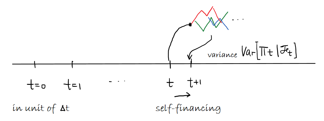
Figure 1: A brief illustration on the modified QLBS environment.

2.3 Specification

In this section, we describe how to set-up the QLBS environment and the necessary numerical procedures.

2.3.1 Environment

The environment is responsible for keeping track of the asset price and portfolio value based on the actions provided by the agent. With a given set of parameters $r,\mu,\sigma,T$, the asset prices are a set of geometrical brownian motion paths $\left\{S_{t}\right\}$ which solves

$$\operatorname{d}S_{t}=\mu S_{t}\operatorname{d}t+\sigma S_{t}\operatorname{d}W_{t}$$

where $W_{t}$ refers to the standard brownian motion according to the filtration $\left\{\mathcal{F}_{t}\right\}$. At each time step $t$, the normalized price $X_{t}=-\left(\mu-\frac{\sigma^{2}}{2}\right)t+\log S_{t}$ and $t$ are provided to the agent, waiting for the response of the hedge position $a_{t}$. Then, the reward $R_{t+1}$, as a conditional expectation specified in Eqn. 8, is computed empirically by averaging samples from a fixed number of additional trajectories under the current policy. At the beginning of each episode, the parameters are adjusted in a random fashion to help the agent explore different settings and help avoid overfitting; the adjustment obeys a Poisson process with intensity $\varUpsilon$.

2.3.2 Agent Parametrization

The agent is fully responsible for determining the hedge position $a_{t}$ under a given normalized price at each time step. The policy $\pi$, whether stochastic or deterministic, depends on these input variables as well as the environment parameters

$$a_{t}\sim\pi\left(X_{t},t;r,\mu,\sigma,T,K,\lambda\right).$$

In pratice, we prefer a stochastic policy since it encourages exploration which is helpful to excape local minima. To further simplify the sampling procedure, we restrict our policy spaces to Gaussian distribution where the agent determines the mean and standard deviation, i.e.

$$\pi=\mathcal{N}\left(\mu_{\pi},\sigma_{\pi}\right)$$

(where the subscripts $\pi$ are used to distinguish these parameters from the environmental ones). The statistics $\mu_{\pi}$ and $\sigma_{\pi}$ are parametrized by two separate neural networks with the Resnet [5] skip-connection structure. The Resnet structure is composed of three parts:

1. Pre-processing $T_{\text{lift}}\left(x\right):=\Xi\left(w_{\text{lift}}^{T}x+b_{\text{lift}}\right)$, that lifts the (8-dimensional) input to the latent dimension by an affine transform and an activation funciton $\Xi$;

2. Chain of transforms $\left\{T^{\left(k\right)}\right\}$ in a fixed-point iteration style, with each transform combining the identity functions and a series of alternating affine transforms $\left\{Z_{l}^{\left(k\right)}\right\}$ and activation $\Xi$, i.e.

   $$T^{\left(k\right)}:=\Xi\circ\left[\text{id}+Z_{n_{k}}^{\left(k\right)}\circ\Xi\circ Z_{n_{k}-1}^{\left(k\right)}\circ\cdots\circ\Xi\circ Z_{1}^{\left(k\right)}\right]$$

3. Post-processing $T_{\text{project}}\left(x\right):=w_{\text{project}}^{T}x+b_{\text{project}}$, that projects the latent representations onto the target space.

Thus, the Resnet realization can be formally written as $T_{\text{project}}\circ T^{\left(k\right)}\circ T^{\left(k-1\right)}\circ\cdots\circ T^{\left(1\right)}\circ T_{\text{lift}}$. We include an illustration in Fig. 2.

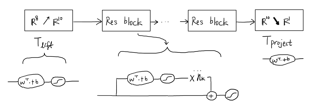
Figure 2: An illustration on a Resnet-motivated network structure.

2.3.3 Learning Algorithm

Since the action space $a_{t}\in\mathbb{R}$ is a continuous space, it is nature to adopt a policy-based method. Here we opt-in the classical REINFORCE algorithm with baseline where the policy components relies on the value estimator to learn quickly and reliably while the value estimator learns from empirical averages of Monte Carlo samples. The value estimator, parameterized by a neural network, uses the same Resnet structure as mentioned in the previous section. We refer to [10] for more details.

In our implementation, the policy network and the value network have the same latent dimension 10 and they are composed of two Resnet blocks with two hidden affine transforms. We use the Adam optimizers to update the networks, one for each, and the learning rate is set to $10^{-4}$ by default.

2.4 Experiments and Results

We include a variety of experiments, starting from a demonstration that shows the agent learns over time, moving to a comparison with the Black-Scholes baseline model, and finally exploring other directions that have a stronger connection to finance.

2.4.1 Demonstration on learning

We start by showing that the policy gradient algorithm has been correctly implemented and the agent learns well over time. The environment parameter is set to $r=0.01,\sigma=0.1,\mu=0,T=5,K=1,S_{0}=1,\Delta t=1,\lambda\in\left\{0,1,2,3\right\},\epsilon=0$ in Sec. 2.4.1, 2.4.2, and 2.4.3 unless otherwise specified. As shown in Fig. 3a, the episodic return flatterns after training for around 3000 steps. It is worth noticing that the cashflow return part

$$\sum_{t=0}^{T-1}\mathbb{E}^{\pi}\left[-\left(1-\frac{t}{T}\right)\Pi_{t}\left(X_{t}\right)+\left(1-\frac{t+1}{T}\right)\Pi_{t}\left(X_{t}\right)\right]=\mathbb{E}^{\pi}\left[\Pi_{0}\left(X_{0}\right)\right]$$

is slightly smaller for a large risk parameter $\lambda$, implying that the agent learns to make a trade-off between the cash-flow and the risk component.

To prepare for learning in a much broader setting, we allow the initial price to be adjusted at a given intensity $\varUpsilon$. We mark out the episodes that the adjustments take place (Fig. 3b) and it seems that the agent can swiftly adapt to the change.

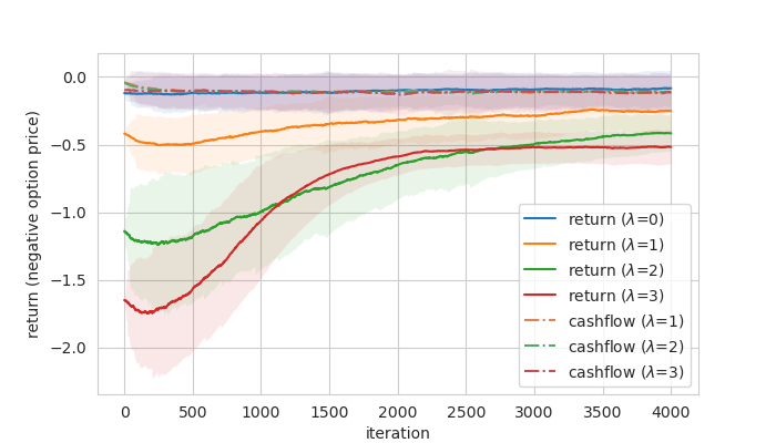
(a) No adjustment on environment parameters. The shade indicates 95% confidence interval. Learning rate set to $10^{-4}$.

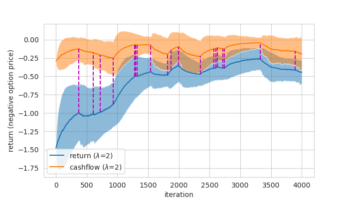
(b) Adjustment parameter (on the initial price) $\varUpsilon=0.005$, indicated by purple lines. The shade indicates 95% confidence interval. Learning rate set to $10^{-4}$.

Figure 3: Exponentially moving average of episodic return.

2.4.2 Influence of risk parameter $\lambda$

We wish to compare the optimal price under different choices of the risk aversion parameter $\lambda$. A priori estimate is that a larger $\lambda$ leads to a higher price learnt, since it penalizes improper hedges harder. To complete the comparision, we also introduce the vanilla BS hedging strategy $\pi_{\text{BS}}$ and learns the episodic return using the same neural network parametrization. The results are shown in Fig. 4. We remind the readers that the option prices are defined as the negative value function, so a lower option price implies a larger return learnt. As we expect, a large $\lambda$ does lead to a higher price, both under BS policy and under the learnt policy. In general, the policy learnt by the neural network parametrization is a bit sub-optimal compared to the BS policy, but it performs better when $\lambda=0.$

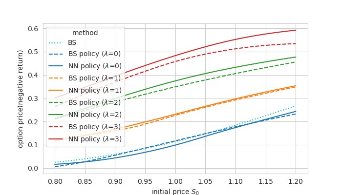
Figure 4: Negative episodic returns as option prices.

2.4.3 Effect of transaction cost

Next, we’d like to examine the effect of transaction costs. As indicated by the self-financing condition (Eqn. 9), a higher trading cost can significantly bias the portfolio value process and consequently increase the optimal price learnt. As shown in Fig. 5, we compare the price and hedge position learnt under different friction parameters $\epsilon$. In general, a larger $\epsilon$ does lead to a higher price learned (shown in the left half) and the hedge position is usually always higher (in the right half).

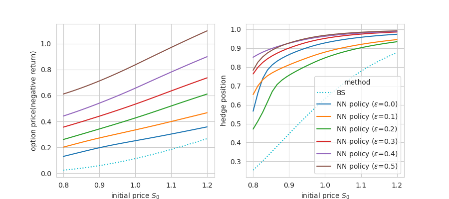
Figure 5: Option priced and hedged under different transaction cost parameters $\epsilon$. $\lambda$ is set to 0.5 to introduce some risk concerns.

2.4.4 Generalization power

As a concluding setting, we wish to parametrize the policy and baseline networks on not only the states but also the environment parameters and examine the generalization power. We pick two set of parameters: $r=0.01,\mu=0,\sigma=0.1,\lambda=0.5,\epsilon=0$ under the first condition while $r=0.02,\mu=0.1,\sigma=0.2,\lambda=1.5,\epsilon=0.1$ under the second condition. We train a policy and baseline under these two conditions mixed, i.e. they have the same probability of being presented, with the switching process being a Poisson process. After training for a while, we refine the agent to learn a third condition where the parameters are set to the arithmic average of the given two conditions. As shown in Fig. 6, we examine the hedging strategy of the agent before and after fine tuning to the third average condition. The result, that the fine tuning does a great improvement, is not surprising since we don’t expect a lot of generalization power. However, one could expect such generalization given enough amount of training time.

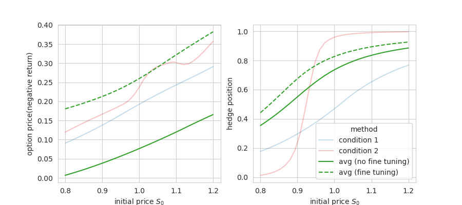
Figure 6: Option priced and hedged under different conditions.

3 RLOP: Replication Learning of Option Pricing

In this section, we propose a novel algorithm that prices a call/put option via portfolio replication, but this method uses a forward view which is fundamentally different from the QLBS approach. The idea is simple: the agent manages a portfolio which yields a reward at the terminal time based on how accurate the portfolio value is compared to the option payoff. This naive idea has the problem that the reward is zero for quite a long time until the maturity, which is usually not good for shaping the agent’s behavior. To deal with this downside, we propose to group a few options as an ensemble so that the agent gets a stream of feedbacks during each episode. To be specific, given a (simulated or historical) path of the asset price $\left\{S_{t}\right\}$, maturity time $T$, and the payoff function $h$, the agent needs to manages (at most) $T$ portfolios $\left\{\Pi_{t}^{\left(i\right)}\right\}_{i=1}^{T}$ at the same time, where the $k$-th portfolio replicates the option that terminals at time step $k$. In other words, for every $i\in\left[t+1,T\right]$, the agent proposes the hedge position $u_{t}^{\left(i\right)}$ based on the current time step $t$, the asset price $S_{t}$, and the balance of the $i$-th portfolio $\Pi_{t}^{\left(i\right)}$. We hold the belief that the agent is able to learn the hedging strategy step by step from small $t$ to the terminal time $T$.

3.1 MDP Formulation

We now rigorously define the aforementioned problem as a MDP. Given a maturity time $i$, the state space consists of tuples containing the time step $t$, the asset price $S_{t}$, and the current portfolio value $\Pi_{t}^{\left(i\right)}$. The action space is $\mathbb{R}$ that contains all possible hedging positions. The transitional probability (density) function is defined as

$$p\left(\left(t,S_{t},\Pi_{t}^{\left(i\right)}\right),u_{t}^{\left(i\right)}\to\left(t^{\prime},S_{t^{\prime}},\Pi_{t^{\prime}}^{\left(i\right)}\right),R_{t+1}\right)=\begin{cases}\delta_{t+1,t^{\prime}}\delta_{\widetilde{\Pi}_{t+1}^{\left(i\right)},\Pi_{t^{\prime}}^{\left(i\right)}}\rho\left(S_{t},S_{t^{\prime}}\right)&t<i\\ 0&t=i\end{cases}$$

where

• the only admissible state is the terminal state when $t>i$, marking the end of this episode;

• $\widetilde{\Pi}_{t+1}^{\left(i\right)}$ refers to the portfolio value determined by the self-financing condition

  $$\widetilde{\Pi}_{t+1}^{\left(i\right)}=e^{r\Delta t}\left(\Pi_{t}-u_{t}^{\left(i\right)}S_{t}\right)+u_{t}^{\left(i\right)}S_{t+1}-\text{TC}\left(u_{t+1}^{\left(i\right)}-u_{t}^{\left(i\right)},S_{t+1}\right)$$

  (which is the same as Eqn. 9);

• $\rho$ characterizes the dynamics of the underlying asset, e.g. the discrete version geometric brownian motion;

• $R_{t+1}=0$ for $t+1<i$ and $R_{i}=H\left(h\left(S_{i}\right),\Pi_{i}^{\left(i\right)}\right)$ where $H$ is a given penalty function that measures how accurate the portfolio value $\Pi_{i}^{\left(i\right)}$ mimics the option payoff $h\left(S_{i}\right)$.

As we mentioned in the previous paragraph, we stack a few pricing tasks together so that the agent gets a reward from the portfolio that recently terminates. For a $T$-term option, we combine $T$ tasks together where the agent is required to learn to price not only the $T$-term one but all $t$-term ones for $t<T$. We briefly illustrate the stucture of RLOP in Fig. 7.

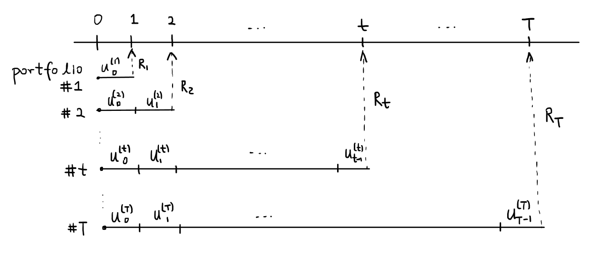
Figure 7: A brief illustration on the RLOP environment.

3.2 Specification

In this section, we describe how to set-up the RLOP environment and the necessary numerical procedures.

3.2.1 Environment

As in the QLBS model, the environment samples a family of asset price trajectories and maintains the portfolio value process. The asset value is assumed to obey the geometrical brownian motion, as in Sec. 2.3.1. We also allows the environment parameters to change at the beginning of each episode according to a Poisson process with intensity $\varUpsilon$.

3.2.2 Agent Parametrization and Learning Algorithm

The agent, i.e. the hedging strategy is parametrized by a Resnet-motivated structure, same in Sec. 2.3.2. The REINFORCE algorithm is adopted to train the agent. One caveat is that there is no need to use a baseline as in the QLBS model, since in this case the reward function is for penalty rather than learning the optimal price.

3.3 Experiments and Results

We include a variety of experiments, including a demonstration that shows the agent learns over time, a comparison with the Black-Scholes baseline model, and a another one on the effect of trading costs.

3.3.1 Demonstration on learning

We use a parameter setting similar to Sec. 2.4.1 where $r=0.01,\sigma=0.1,\mu=0,T=5,K=1,S_{0}=1,\Delta t=1$. The agent is trained under no transaction cost with a fixed initial asset value and the training curve is flat after around 8000 steps, shown in Fig. 8a. Similar to the QLBS setting, we introduce adjustment to the parameters (i.e. the initial asset value in the experiments to follow) by a Poisson process. We mark where the adjustment occurs in the bottom half of the figure by purple triangles.

We also compare the optimal hedging strategy learnt with the BS predictions. In general, the hedging curve should have a greater slope for a smaller remaining time which implies that the price of the option is more sensitive to the underlying asset price. As expected, both the learnt position and the BS position show a greater slope when approaching the terminal time. The one learnt by our RL agent is slightly insensitve to the time variable.

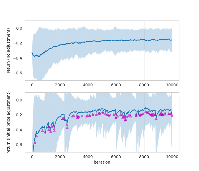
(a) Episodic return improves during training. Top figure: no adjustment on the initial price $S_{0}$; bottom figure: the initial price is adjusted via a Poisson process.

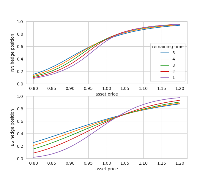
(b) Optimal hedge position learnt compared with BS predictions (Eqn. 3).

Figure 8: Demonstration the RLOP model learning curve and a comparison to the BS predictions.

3.3.2 Effect of transaction cost

We proceed to measure how the transaction cost can effect the optimal hedging strategy. We use the same setting as laid out in Sec. 2.4.3 where $\epsilon$ is the friction parameter. We plot the optimal hedging position learnt under different $\epsilon$ in Fig. 9. The general trend is that a large $\epsilon$ discourages hedging amounts, since it leads to a higher trading cost on average. A higher friction also leads to a larger distinction between positions at different times, which implies that in an illuquid market, we need to value the time variable more than in a liquid one.

Figure 9: Optimal hedging strategy learnt under different transaction costs.

4 Conclusion and Discussion

In this project, we construct the modified QLBS and RLOP as two mathematically sound environments that enable RL methods in the field of option pricing. We specify the environment details as well as how the agent is parametrized and trained. We provide a few numerical experiments which compare the learned optimal hedging against the BS predictions. We also study how the factors affect the optimal price and position. We hope that this work can inspire and motivate more research into the cross-discipline study between finance and machine learning.

We would like to discuss a few possible future directions, starting from the financial aspects. We focus on European call options in this report, but in general, it shall also apply to the put option or other options that can only exercise at the terminal time. It is not clear whether the QLBS or RLOP model can generalize to the American or even swing options that are useful in electricity trading. Besides, the transaction cost model proposed in Sec. 1.3 can be greatly improved to allow fine models on the order density, or even influence on the mid price.

There are also a few open questions on the mathematics side. It could be beneficial to analyze the theoretical optimal hedging strategy in the discrete time model. We have provided an analogous to the stochastic integral in the earlier sections, which might help in analyzing the temporal discretization error. Besides, the modified QLBS reward function (Eqn. 7) is no longer time translational invariant, so one has to train a new model if the maturity time of the option changes. It would be a great improvement if one finds an equivalent or a similar formulation where the value function is translational invariant while giving homogeneous rewards over time.

We also have a few comments on the learning/sampling algorithms. One common drawback of the two methods is that the computational complexity scales quadratically as the maturity time $T$. The modified QLBS model requires computing a conditional expectation at each time step, which is not of constant cost. The RLOP model stacks $T$ pricing tasks together, each lasting one more period than the previous one, leading to a quadratic cumulative cost. Another issue is that we use REINFORCE with baseline as the learning algorithm, which can be replaced by the actor-critic (or even the soft version) to improve performance. More time is appreciated since we have limited time in the project to try different possibilities.

There are controversial conclusions as far as what the numerical experiments show. In general, the agents learn to price a higher price if the current price $S_{t}$ is higher, or the risk aversion parameter $\lambda$ (or the friction parameter $\epsilon$) is larger. However, the two models predict the optimal hedging strategy differently, especially when large friction is anticipated. The modified QLBS agent prefers to hedge more than the frictionless case while the RLOP agent inclines to hedge less. This discrepancy might be the key to understanding the difference between these two models and eventually the option pricing problem.

References

- [1] A. Fathan and E. Delage, Deep reinforcement learning for optimal stopping with application in financial engineering, arXiv preprint arXiv:2105.08877, (2021).
- [2] T. Grassl, A reinforcement learning approach for pricing derivatives, 2010.
- [3] I. Halperin, Qlbs: Q-learner in the black-scholes (-merton) worlds, The Journal of Derivatives, 28 (2020), pp. 99–122.
- [4] , Distributional offline continuous-time reinforcement learning with neural physics-informed pdes (sciphy rl for doctr-l), arXiv preprint arXiv:2104.01040, (2021).
- [5] K. He, X. Zhang, S. Ren, and J. Sun, Deep residual learning for image recognition, in Proceedings of the IEEE conference on computer vision and pattern recognition, 2016, pp. 770–778.
- [6] Y. Li, C. Szepesvari, and D. Schuurmans, Learning exercise policies for american options, in Artificial Intelligence and Statistics, PMLR, 2009, pp. 352–359.
- [7] S. Marzban, E. Delage, and J. Y. Li, Deep reinforcement learning for equal risk pricing and hedging under dynamic expectile risk measures, arXiv preprint arXiv:2109.04001, (2021).
- [8] M. Musiela, Martingale Methods in Financial Modelling by Marek Musiela, Marek Rutkowski., Stochastic Modelling and Applied Probability, 36, Springer Berlin Heidelberg, Berlin, Heidelberg, 2nd ed. 2005. ed., 2005.
- [9] S. E. Shreve et al., Stochastic calculus for finance II: Continuous-time models, vol. 11, Springer, 2004.
- [10] R. S. Sutton and A. G. Barto, Reinforcement learning: An introduction, MIT press, 2018.
- [11] A. Tamar, Y. Chow, M. Ghavamzadeh, and S. Mannor, Policy gradient for coherent risk measures, Advances in neural information processing systems, 28 (2015).