UoA

March 11, 2024

Gravitational Waves From No-Scale Supergravity

Vassilis C. Spanos and Ioanna D. Stamou

National and Kapodistrian University of Athens, Department of Physics,
Section of Nuclear and Particle Physics, GR–15784 Athens, Greece

In this paper we study four concrete models, based on no-scale supergravity with SU(2,1)/SU(2)$\times$ U(1) symmetry. We modify either the Kähler potential or the superpotential, which are related to the no-scale theory with this symmetry. In this scenario, the induced Gravitational Waves, are calculated to be detectable by the future space-based observations such as LISA, BBO and DECIGO. The models under study are interrelated, as they all yield the Starobinsky effective-like scalar potential in the unmodified case. We evaluate numerically the scalar power spectrum and the stochastic background of the Gravitational Waves, satisfying the observational Planck cosmological constraints for inflation.

1 Introduction

The detection of the Gravitational Waves (GWs) is undeniably regarded as a milestone in cosmology. The GWs emitted by a binary black hole merges, reported by the LIGO and Virgo collaborations [1, 2, 3, 4, 5], draw attention to both experimental and theoretical researches for exploring the stochastic background of GWs. The signal of the GWs is expected to be detectable by future space-based GW interferometers such as LISA, BBO and DECIGO[6, 7].

The detection of these events by the LIGO/Virgo collaborations has been rekindled the old study of Primordial Black Holes (PBHs)[8, 9, 10, 11]. Specifically, it has been claimed that the PBHs, which are formed during radiation dominated epoch, can be considered as reliable candidates for a large, or the whole amount of the Dark Matter (DM) of the Universe[12, 13, 14, 15, 16, 17, 18, 19, 20, 21, 22, 23, 24, 25, 26, 27]. In this case, there is a strong possibility to detect induced GWs’ signals, which are generated during the radiation phase and will be available in the future from the aforementioned observations. The contribution of the first order scalar perturbations, to the generation of second order perturbations associated to the GWs, has already been studied in detail [28, 29, 30, 31, 32, 33, 34].

Several mechanisms for producing enhancement in the scalar power spectrum have been proposed in the literature. In the case of the single field inflation, the mechanism associated to the presence of an inflection point has been already studied extensively [13, 14, 15, 16, 17, 18, 19, 20, 21, 22, 23, 26, 27]. At the inflection point, both first and second derivatives of the effective scalar potential become approximately zero. This feature in the effective scalar potential, significantly decreases the velocity of the inflaton. This decrease is imprinted in a peak in power spectrum. The slow-roll approximation fails to give the correct results and one has to solve numerically the exact equation of the field perturbations, because the slow-roll parameter $\eta$ growths significantly. In this work we will consider this mechanism for producing such amplifications. However, alternative mechanisms have been proposed regarding single field inflation. One of them is models with a feature like steps in the potential[35, 36, 37, 38]. Moreover, models with ultra slow-roll inflation have been studied [39, 40]. Two field inflationary model have also been proposed [41, 24, 42, 43, 44].

The relation between the first and second order perturbations, that is the scalar and the tensor power spectrum, gives the insight to study the GWs by analysing and measuring only the scalar power spectrum [28, 29, 30, 31, 32, 33, 45, 46, 47]. There are numerous studies based on this scenario [24, 25, 48, 43, 49, 50, 51, 52, 53, 54, 55, 37, 56] and we briefly discuss some of them. In Refs. [24, 25] the authors study two scalar field models with a non-canonical kinetic term. Other two-field models, in order to generate GWs have been studied in Refs. [24, 25, 42, 43, 48]. The production of GWs within a single field inflation has been considered in Refs. [56, 55, 50, 37].

Supergravity (SUGRA) models can provide us with inflationary potentials compatible with observational data. To this end, a significant enhancement in the scalar power spectrum as described above, can occur [21, 22, 18, 17, 26, 27]. In particular, it has been claimed that no-scale theory can be regarded as a theory worthy of consideration, in order to study enhancement in power spectrum [21, 22]. This theory treats many problematic issues such as the fine-tuning in order to obtain a vanishing cosmological constant and it gives a natural solution to the $\eta$ problem [57, 58, 59, 60, 61].

In [22] a mechanism to produce PBHs was proposed, based on the breaking of the non-compact SU(2,1)/SU(2)$\times$ U(1) symmetry. It is proved that, the effective scalar potentials related to inflation, not only can explain the production of PBHs, but also they can conserve the transformation laws, related to the coset SU(2,1)/SU(2)$\times$ U(1). In this work we will consider these potentials, in order to explain the generation of GWs and we will numerically evaluate the energy density. Moreover, we generate GWs by modifying the kinetic term in the Lagrangian and keeping the superpotentials, which lead to the Starobinsky-effective potential such as the Wess-Zumino or the Cecotti, unchanged. All the models present in this work are in consistence with the Planck constraints of the spectral index $n_{s}$ and the tensor-to-scalar ratio $r$ [62, 63].

The layout of the paper is as follows: In section 2 we briefly review some basic aspects for the SUGRA theory and the perturbation theory, which are used in our analysis. In section 3 we explain how the enhancement of power spectrum can be produced in the framework of no-scale theory. In section 4 we present the GWs for our analysis. Finally, in section 5 we give our conclusions and perspectives.

2 Basic Considerations

In this section we discuss two basic considerations used in our analysis. The first is an introduction to SUGRA theory, which is relevant to the inflation models we will employ below. The second is about the general tools used for studying the field perturbations during inflation.

2.1 General Aspect Of Supergravity

In this subsection we present some basic aspects of SUGRA and particularly the no-scale theory. The SUGRA Lagrangian coupled to matter is given in the following expression

$$\mathcal{L}=\frac{1}{2}R-K^{\Phi\bar{\Phi}}\partial_{\mu}\Phi\partial^{\mu}\bar{\Phi}-V(\Phi,\bar{\Phi})\,,$$ (2.1)

where $K$ denotes the Kähler potential, $W$ is the superpotential and the indices $\Phi$ and $\bar{\Phi}$ denote the derivatives in respect to the corresponding fields. We remark that throughout this study we work in reduced Planck units ($M_{P}=1$).

The F-term of scalar potential is given as follows

$$V=e^{K}(D_{\Phi}WK^{\bar{\Phi}\Phi}D_{\bar{\Phi}}\bar{W}-3|W|^{2})\,,$$ (2.2)

where

$$D_{\Phi}W=\frac{\partial W}{\partial\Phi}+\frac{\partial K}{\partial\Phi}W$$ (2.3)

is the Kähler convariant derivative.

The minimal no-scale model is given by the Kähler potential in the present of a single chiral field $\Phi$ [57, 58, 59, 60, 61]

$$K=-3\ln(\Phi+\bar{\Phi}).$$ (2.4)

By considering this Kähler potential, one can notice that the term $-3|W|^{2}$ in Eq.(2.2) is vanishing because of the following expression [57]

$$K^{\Phi\bar{\Phi}}K_{\Phi}K_{\bar{\Phi}}=3.$$ (2.5)

In the case of non-compact symmetry SU(2,1)/SU(2)$\times$ U(1), a no-scale supergravity model is described by the following two equivalent Kähler potentials [64]

$$K=-3\ln\left(T+\bar{T}-\frac{|\varphi|^{2}}{3}\right)$$ (2.6)

and

$$K=-3\ln\left(1-\frac{|y_{1}|^{2}}{3}-\frac{|y_{2}|^{2}}{3}\right)$$ (2.7)

where $y_{1}$, $y_{2}$, $T$ and $\varphi$ are chiral fields. The Kähler potential in $(y_{1},y_{2})$ basis is related to this in the $(T,\varphi)$ basis, as analyzed in [65]. The relevant transformation is

$$y_{1}=\Big{(}\frac{2\varphi}{1+2T}\Big{)},\quad y_{2}=\sqrt{3}\Big{(}\frac{1-2T}{1+2T}\Big{)}\,,$$ (2.8)

while its inverse is

$$T=\frac{1}{2}\Big{(}\frac{1-y_{2}/\sqrt{3}}{1+y_{2}/\sqrt{3}}\Big{)},\quad\varphi=\Big{(}\frac{y_{1}}{1+y_{2}/\sqrt{3}}\Big{)}\,.$$ (2.9)

For a given superpotential, in the $(y_{1},y_{2})$ basis, we can derive the corresponding in $(T,\varphi)$ by using the following relation [65]

$$W(T,\varphi)\rightarrow\bar{W}(y_{1},y_{2})=\left(1+y_{2}/\sqrt{3}\right)^{3}W\,.$$ (2.10)

In order to present inflationary models which are in agreement with the current observational data on CMB anisotropies [62, 63], we consider the Starobinsky-type potential. We note that in [62, 63] the $\mathcal{R}^{2}$ inflationary models are in accordance with the current data. Interestingly, the no-scale theory described above, provides us with potentials of this kind (Starobinsky-like potential) [66, 67]. Furthermore, there are other supergravity models, which can lead to Starobinsky-like potential as well. We briefly mention the $\alpha$-attractor models, which are described in [68, 69, 70]. In these models the Eq. (2.7) is multiplied by a term $\alpha$, which can be different to one:

$$K=-3\alpha\ln\left(1-\frac{|y_{1}|^{2}}{3}-\frac{|y_{2}|^{2}}{3}\right).$$ (2.11)

As a result the condition (2.5) is not conserved. However, these models have other interesting features, e.g. they are invariant under the conformal transformations [68, 69, 70].

In our analysis, the Starobinsky-like effective scalar potential can be derived with two ways from no-scale theory, as it is described below. One is this of the Wess-Zumino model [67]

$$W=\frac{\hat{\mu}}{2}\varphi^{2}-\frac{\lambda}{3}\varphi^{3}\,,$$ (2.12)

where $\hat{\mu}$ is a mass term and $\lambda$ a trilinear coupling in the Lagrangian. This is written in the $(T,\varphi)$ basis. In order to get the Starobinsky-like effective scalar potential, we use the Eq.(2.2) and we assume that the inflationary direction is ${\textrm{Im}}\varphi={\textrm{Im}}T=0$ and ${\textrm{Re}}T=c$. We define $\hat{\mu}=\mu\sqrt{c/3}$. In addition, in order to evaluate the effective potential we need to fix the non-canonical kinetic term. To do this we use the following redefinition of the field

$$\varphi=\sqrt{3}\tanh\left(\frac{\phi}{\sqrt{6}}\right)$$ (2.13)

where $\phi$ is the field with fixed the non-canonical kinetic term. From Eq.(2.2) we get

$$V=\mu^{2}e^{-\sqrt{2/3}x}\sinh^{2}\left(\frac{\phi}{\sqrt{6}}\right),$$ (2.14)

where we have assumed $\lambda/\mu=1/3$.

The superpotential in Eq.(2.12) can be written in $(y_{1},y_{2})$ basis, using the Eqs. (2.9) and (2.10) [65]. Hence, we get

$$W=\frac{\hat{\mu}}{2}\Big{(}y_{1}^{2}+\frac{y_{1}^{2}y_{2}}{\sqrt{3}}\Big{)}-\lambda\frac{y_{1}^{3}}{3}$$ (2.15)

and the kinetic term is fixed using the redefinition

$$y_{1}=\sqrt{3}\tanh\left(\frac{\phi}{\sqrt{6}}\right)\,,$$ (2.16)

where the Starobinsky effective scalar potential appears assuming that the $y_{1}$ is the inflaton field and $y_{2}$ is the modulo. The resulting effective scalar potential is the same with this derived in the $(T,\varphi)$ basis.

Alternatively, the Starobinsky-like potential can be derived by the Cecotti superpotential as given in $(T,\varphi)$ basis as [66]

$$W=\sqrt{3}\,m\,\varphi\,\left(T-\frac{1}{2}\right)\,,$$ (2.17)

where $m$ is a mass term. The Starobinsky effective scalar potential arises thought the direction $\varphi=\text{Im}T=0$. In order to have canonical kinetic terms, one has to use the field redefinition

$$T=\frac{1}{2}e^{\sqrt{\frac{2}{3}}\phi}\,.$$ (2.18)

In general, the kinetic term can be fixed by the transformation

$$\frac{1}{2}\partial_{\mu}\phi\partial^{\mu}\phi=K_{\chi\chi}\partial_{\mu}x\partial^{\mu}\chi\Rightarrow\frac{d\phi}{d\chi}=\sqrt{2K_{\chi\chi}}\,.$$ (2.19)

Although the relation  (2.19) in the case of the Kähler potentials (2.6) and (2.7) yields analytical solution, it is also generally useful even in the cases that there is no analytical solution. In the following, we will consider both analytical and numerical solutions of Eq. (2.19).

The superpotential in Eq. (2.17) can be written in the $(y_{1},y_{2})$ basis as

$$W=m\Big{(}-y_{1}y_{2}+\frac{y_{2}y_{1}^{2}}{\sqrt{3}}\Big{)}$$ (2.20)

and as before the redefinition for the canonical kinetic term is

$$y_{1}=\sqrt{3}\tanh\left(\frac{\phi}{\sqrt{6}}\right)\,,$$ (2.21)

with $y_{1}$ being the inflaton field and $y_{2}$ the modulo. If we evaluate the effective potential, we can obtain the same Starobinsky-like potential in both bases $(T,\varphi)$ and $(y_{1},y_{2})$.

Therefore, there is an important equivalence between the models of Wess-Zumino and Cecotti, as they can provide us with Starobinsky-like potential, when they are embedded in no-scale theory [64]. Moreover, when we study the forms written in $(y_{1},y_{2})$ basis in Eq.(2.7) and the corresponding superpotential given in (2.15) and (2.20) we can obtain that these models obey the symmetry identified by the matrix

$$U=\begin{bmatrix}\alpha&\beta&0\\ -\beta^{*}&\alpha^{*}&0\\ 0&0&1\end{bmatrix}\,,$$ (2.22)

where $\alpha,\beta\in\mathbb{C}$ and $|\alpha|^{2}+|\beta|^{2}=1$. By this matrix and the analysis shown in Ref. [64] we can obtain the following transformation laws for the fields

$$y_{1}\rightarrow\alpha y_{1}+\beta y_{2},\quad y_{2}\rightarrow-\beta^{*}y_{1}+\alpha^{*}y_{2}.$$ (2.23)

This symmetry is analyzed in [64]. In the next section we will present models that satisfies this symmetry.

2.2 Curvature Perturbations

The equation of motion of the inflaton field is

$$\phi^{\prime\prime}+3\phi^{\prime}-\frac{1}{2}\phi^{\prime 3}+\left(3-\frac{1}{2}\phi^{\prime 2}\right)\frac{d\ln V(\phi)}{d\phi}=0\,,$$ (2.24)

where primes denote the derivative in efold time.

The general Friedmann-Robertson-Walker (FRW) metric written in the conformal Newtonian gauge is [71, 72]

$$ds^{2}=-a^{2}\left(1+2\Phi\right)d\tau^{2}+a\left((1+2\Psi)\delta_{ij}+\frac{1}{2}h_{ij}\right)dx^{i}dx^{j}\,,$$ (2.25)

where $\tau$ is the conformal time, $a$ is the scale factor, $h_{ij}$ are tensor perturbations, $\Phi$ and $\Psi$ are the Bardeen potentials, which are equal in the absence of anisotropy in the stress energy tensor. Assuming that the perturbation of the field is $\phi+\delta\phi$, the equation of the curvature perturbation takes the form [73]

$${\delta\phi^{\prime\prime}=-\left(3-\frac{1}{2}\phi^{\prime 2}\right)\delta\phi^{\prime}-\frac{1}{H^{2}}\frac{d^{2}V}{d\phi^{2}}\delta\phi-\frac{k^{2}}{a^{2}H^{2}}\delta\phi+4\Psi^{\prime}\phi^{\prime}-\frac{2\Psi}{H^{2}}\frac{dV}{d\phi}}\,,$$ (2.26)

where the Bardeen potential $\Psi$ results from the equation

$${\Psi^{\prime\prime}=-\left(7-\frac{1}{2}\phi^{\prime 2}\right)\Psi^{\prime}-\left(2\frac{V}{H^{2}}+\frac{k^{2}}{a^{2}H^{2}}\right)\Psi-\frac{1}{H^{2}}\frac{dV}{d\phi}\delta\phi\,.}$$ (2.27)

With $H$ we denote the Hubble parameter, which is

$${H^{2}=\frac{V}{(3-\frac{1}{2}{\phi^{\prime}}^{2})}\,.}$$ (2.28)

The initial condition for the perturbation, assuming Bunch-Davies vacuum, is

$$aQ\rightarrow\frac{e^{-ik\tau}}{\sqrt{2k}}\,,$$ (2.29)

where $Q$ is the Mukhanov-Sassaki variable. The complete expressions for the initial conditions for the perturbation, as well as the initial conditions for the Bardeen potential are

$$\begin{split}{\delta\phi_{ic}=\frac{1}{\sqrt{2k}}\frac{1}{a_{ic}},\quad\left(\delta\phi^{\prime}\right)_{ic}=-\frac{1}{a_{ic}\sqrt{2k}}\left(1+i\frac{k}{a_{ic}H_{ic}}\right)}\end{split}$$ (2.30)

and

$$\begin{split}\Psi_{ic}=&\frac{1}{2\left(\varepsilon_{H,ic}-\frac{k^{2}}{a_{ic}^{2}H_{ic}^{2}}\right)}\left(\phi^{\prime}_{ic}\delta\phi^{\prime}_{ic}+\delta\phi_{ic}\left[3\left(\phi^{\prime}\right)_{ic}+\frac{1}{H_{ic}^{2}}\left(\frac{dV}{d\phi}\right)_{ic}\right]\right)\\ \Psi^{\prime}_{ic}=&\frac{1}{2}\left(\phi^{\prime}\right)_{ic}\delta\phi_{ic}-\Psi_{ic}\,.\end{split}$$ (2.31)

With the indices $ic$ we denote the initial conditions and with the $\varepsilon_{H}$ we denote the slow roll parameter

$$\varepsilon_{H}=\frac{1}{2}\phi^{\prime 2}.$$

We note that these equations are valid for a Lagrangian with a canonical kinetic term. Otherwise one should take into account the field transformation in order to fix the canonical kinetic term, as we have mentioned in the previous subsection in Eq.(2.19).

Using Eqs. (2.24) -(2.28) we can evaluate the power spectrum as

$$P_{R}=\frac{k^{3}}{2\pi^{2}}\left|R_{k}\right|^{2},$$ (2.32)

where $k$ is the comoving wavenumber of the Fourier mode and

$$R_{k}=\Psi+\frac{\delta\phi}{\phi^{\prime}}\,.$$ (2.33)

The numerical procedure, we follow is descibed in Refs. [21, 22].

There are many works where the analytical evaluation of enhanced power spectrum has been studied, such as [36, 37, 40]. The power spectrum in the vicinity of the peak can be approximated analytically by the power-law spectrum which is given as [74, 75]:

$$P_{R}=\begin{cases}0&\text{if $k<k_{peak}$}\\ P_{0}\left(\frac{k}{k_{peak}}\right)^{-n}&\text{if $k>k_{peak}$}\,\,,\end{cases}$$ (2.34)

where $k_{peak}$ is the comoving wavenumber of the peak. $P_{0}$ is related to the peak amplitude and $n$ is related to the spectral index. In the following we present both numerical and analytical results for the sake of comparison.

The models we study in this work are based on $\mathcal{R}^{2}$ inflation and are consistent with the current observational data of inflation. To this end, we use the slow-roll parameter $\eta_{H}$, defined as

$$\eta_{H}=\varepsilon_{H}-\frac{1}{2}\frac{d\ln\varepsilon_{H}}{dN}\,.$$ (2.35)

The slow-roll parameters $\varepsilon_{V}$ and $\eta_{V}$ are defined also in terms of the inflationary potential as

$$\varepsilon_{V}=\frac{1}{2}\left(\frac{V^{\prime}(\phi)}{V(\phi)}\right)^{2},\quad\eta_{V}=\frac{V^{\prime\prime}(\phi)}{V(\phi)}\,,$$ (2.36)

where primes denote the derivatives in respect of the field $\phi$. The spectral index is defined as

$$n_{s}-1=\frac{d\ln P_{R}}{d\ln k}\,.$$ (2.37)

In terms of slow roll conditions for the prediction of the observable $n_{s}$, we get

$$n_{s}\simeq 1+2\eta_{V}-6\varepsilon_{V}\,.$$ (2.38)

The prediction for the ratio tensor-to-scalar $r$ are

$$r\simeq 16\varepsilon_{V}.$$ (2.39)

The corresponding values for these quantities, which are evaluated at the pivot scale of $k_{*}=0.05Mpc^{-1}$ are [63]

$$n_{s}=\begin{cases}0.9659\pm 0.0041&\text{Planck TT,TE,EE+lowEB+lensing}\\ 0.9651\pm 0.0041&\text{Planck TT,TE,EE+lowEB+lensing+BK15}\\ 0.9668\pm 0.0037&\text{Planck TT,TE,EE+lowEB+lensing+BK15+BAO}\end{cases}$$ (2.40)

and

$$r<\begin{cases}0.11&\text{Planck TT,TE,EE+lowEB+lensing}\\ 0.061&\text{Planck TT,TE,EE+lowEB+lensing+BK15}\\ 0.063&\text{Planck TT,TE,EE+lowEB+lensing+BK15+BAO}\,.\end{cases}$$ (2.41)

In the following we present the predictions for the observables of the proposed models and we will check their consistency against the Planck data.

3 Gravitational Waves from the No-Scale models

Below we will study how modifications in the superpotential or in the Kähler potential can be used in order to explain the generation of GWs. We present two different ways to produce such peaks in power spectrum, which as we will see it is related to the spectrum of GWs. The first is by modifying the Wess-Zumino and Cecotti superpotential, given in Eqs. (2.12),  (2.15), (2.13) and  (2.17). The second is by modifying the Kähler potential, meaning the kinetic term on the Lagrangian, taking into account that both Wess-Zumino superpotential and Cecotti superpotential are unchanged. Therefore, we present two different ways in order to get significant peaks in the power spectrum by conserving (modifying superpotentials) and breaking (modifying Kähler potential) the SU(2,1)/SU(2)$\times$ U(1) symmetry. All models give the Starobinsky effective scalar potential in the unmodified case.

3.1 Modifying the superpotential

It was shown that the non-compact SU(2,1)/SU(2)$\times$ U(1) symmetry leads to the same Starobinsky-like effective scalar potential, demonstrating an important equivalence between the different models [64]. Moreover, it can be shown that this symmetry can be preserved [22] under proper modification of the superpotential, in order to generate a peak in power spectrum and produce significant amount of the PBHs in the Universe. Therefore, we consider the no-scale supergravity coset SU(2,1)/SU(2)$\times$ U(1). This coset can be identified by two equivalent forms of the Kähler potential

$$\begin{split}K=-3\ln(1-\frac{|y_{1}|^{2}}{3}-\frac{|y_{2}|^{2}}{3})\\ K=-3\ln(T+\bar{T}-\frac{|\varphi|^{2}}{3})\,,\end{split}$$ (3.1)

which can be written in two basis, the $(T,\varphi)$ and $(y_{1},y_{2})$.

First, by a proper modification of the Wess-Zumino model, we can derive the same effective scalar potential in both $(T,\varphi)$ and $(y_{1},y_{2})$ basis. The superpotential adopted in Ref. [22], for modified the Wess-Zumino model in $(y_{1},y_{2})$ basis, is

$$W=\left[\frac{\hat{\mu}}{2}\left(y_{1}^{2}+\frac{y_{2}^{2}y_{1}}{\sqrt{3}}\right)-\lambda\frac{y_{1}^{3}}{3}\right]\left[1+e^{-b_{1}y_{1}^{2}}\left(c_{1}{y_{1}}^{2}+c_{2}{y_{1}}^{4}\right)\right]\,,$$ (3.2)

where $\hat{\mu}$, $\lambda$, $b_{1}$, $c_{1}$ and $c_{2}$ are free parameters, fixed by observations. The effective scalar potential can be calculated by using Eq. (2.2) and the redefinition of the field, which is given in Eq. (2.16). Using this modification the resulting effective scalar potential is not affected by the transformations $y_{1}\rightarrow-y_{1}$ and $y_{2}\rightarrow-y_{2}$. Alternatively, using $y_{1}\rightarrow-y_{2}$ and $y_{2}\rightarrow y_{1}$, one can derive the same effective scalar potential, in the inflationary direction $y_{2}={\textrm{Im}}\,y_{1}=0$, by fixing the non-canonical kinetic term as

$$y_{1}=-\sqrt{3}\tanh\left(\frac{\phi}{\sqrt{6}}\right)\,.$$ (3.3)

This analysis is presented in [64].

Figure 1: The effective potential (solid line) for the superpotential in Eq. (3.2) with the choice of parameters $\lambda/\mu=1/3$, $c_{1}=1.9$, $c_{2}=-0.73$ and $b_{1}=3.9615$. The dashed like corresponds to the Starobinsky potential.

The superpotential in Eq. (3.2) can be written in the $(T,\varphi)$ basis, if one considers the Eq. (2.10). Hence

$$W=\left(\frac{\hat{\mu}}{2}\varphi^{2}-\frac{\lambda}{3}\varphi^{3}\right)\left(1+e^{-b_{1}\left(\frac{2\varphi}{1+2T}\right)^{2}}\left[c_{1}\left(\frac{2\varphi}{1+2T}\right)^{2}+c_{2}\left(\frac{2\varphi}{1+2T}\right)^{4}\right]\right)\,,$$ (3.4)

where $\varphi$ is the inflaton field and $T$ is the modulo. This yields the same effective scalar potential as in Eq. (3.2) using the redefinition of the field (2.13), in order to get canonical kinetic terms. In Fig. 1 we present the effective scalar potential given for the superpotential (3.2) (or equivalently Eq.(3.4)). The details for this calculation are described in Appendix A. In order to derive this potential we redefine the field in order to have canonical kinetic terms. We notice that there is a region around $\phi\approx 1.4$, where there is a near inflection point. We expect that this feature can be imprinted in the scalar power spectrum. On the other hand, there are many mechanisms in order to obtain an enhancement in scalar power spectrum, such as two field models, models with bumpy features[76, 77]. In Appendix B there is a comparison between some models. In Fig. 1 we also depict the case of $c_{1}=c_{2}=0$ which correspond to the Starobinsky potential.

In addition to that, by a proper modification in Cecotti superpotential, given in (2.17), we can produce significant peak in the power spectrum in the $(y_{1},y_{2})$ basis. In Ref.[22] the following superpotential is considered

$$W=m\left(-y_{1}y_{2}+\frac{y_{2}y_{1}^{2}}{l\sqrt{3}}\right)\left(1+c_{3}e^{-b_{2}{y_{1}}^{2}}{y_{1}}^{2}\right)\,,$$ (3.5)

where $m$, $l$, $c_{3}$, $b_{1}$ are the parameters of the model. This choice of modification is made for keeping the resulting effective scalar potential unchanged under the transformations $y_{1}\rightarrow-y_{1}$, $y_{2}\rightarrow-y_{2}$. Also, if one considers the case of exchanging the modulo and the inflaton field by changing $y_{1}\rightarrow-y_{2}$ and $y_{2}\rightarrow y_{1}$, the effective scalar potential remains the same. For more detail see Refs. [22].

In the $(T,\varphi)$ basis, the superpotential (3.5) takes the following form using Eq. (2.10)

$$W=\frac{\sqrt{3}}{2}m\varphi\Big{(}\frac{1}{2}-T\Big{)}\left(-1-2T-\frac{1-2T}{l}\right)\left[1+3c_{3}e^{-3b_{2}\left(\frac{1-2T}{1+2T}\right)^{2}}\left(\frac{1-2T}{1+2T}\right)^{2}\right]\,.$$ (3.6)

This gives the same effective scalar potential as in Eq. (3.5), if we consider the redefinition of the field of Eq. (2.18).

The superpotentials (3.2) and (3.5) not only preserve the same resulting effective scalar potential in both $(y_{1},y_{2})$ and $(T,\varphi)$ basis, by the transformation given in Eq. (2.10), but also they can produce significant enhancement in the power spectra, explaining the production of PBHs, as shown in [22]. In the following we will show that these peaks can also produce GWs spectra sizeable enough to be detected in the corresponding experiments. These peaks are related to the inflection points in effective scalar potential, which one can find by a proper choice of parameters, as shown in [22].

To sum up, the new terms that are present in Eqs.(3.2) and (3.5) not only preserve the transformation laws of the symmetry SU(2,1)/SU(2)$\times$ U(1) as given in Eq. (2.23), but also result to a significant enhancement in scalar power spectrum. Hence, these modifications have the following interesting properties. First, they conserve the SU(2,1)/SU(2)$\times$ U(1) symmetry. Second, they give the same form of the potential in both bases $(y_{1},y_{2})$ and $(T,\varphi)$. Third, they satisfy the no-scale condition (2.5), in order to ensure the vanishing of the cosmological constant. Last but not least, they can result to an inflection point under proper choice of parameters and finally, therefore can yield to a significant amount of PBHs and GWs.

3.2 Modifying the Kähler potential

In the previous section we study the generation of significant peaks in power spectrum by modifying well-known superpotentials, which yield to the Starobinsky-like effective scalar potential. These significant peaks can be also presented by modified only the Kähler potential and keeping the superpotential unchanged. Hence, this amplification can be found via breaking the SU(2,1)/SU(2)$\times$ U(1) symmetry by adding extra terms in the kinetic part of the Lagrangian. In this section we present two models in order to produce such peaks, one by keeping the Wess-Zumino superpotential (2.12) unchanged and the other by keeping the Cecotti superpotential unchanged (2.17).

In a previous work it was shown that sizable amplification in the power spectrum can be produced through the scheme[21]

$$K=-3\ln(T+\bar{T}-\frac{\varphi\bar{\varphi}}{3}+c_{3}e^{-b_{3}(\varphi+\bar{\varphi})^{2}}(\varphi+\bar{\varphi})^{4})\,,$$ (3.7)

$$W=\frac{\hat{\mu}}{2}\varphi^{2}-\frac{\lambda}{3}\varphi^{3}\,,$$ (3.8)

where $c_{3}$ and $b_{3}$ are free parameters of the model. This model has to deal with just an extra parameter $b_{3}$, which gives us both peaks in power spectrum and the correct prediction of spectral index $n_{s}$ and the tensor-to-scalar ratio $r$. The advantage of this model is that it leads to a reduced level of fine-tuning, as we will see later.

Also it is considered that the superpotential is given by the Cecotti form, Eq.  (2.17). Specifically, we have

$$K=-3\ln(T+\bar{T}-\frac{\varphi\bar{\varphi}}{3}+F(T+\bar{T},\varphi+\bar{\varphi}))$$ (3.9)

$$W=\sqrt{3}m\varphi\left(T-\frac{1}{2}\right)$$ (3.10)

where $F(T+\bar{T},\varphi+\bar{\varphi})$ is a function of both chiral fields. Choosing

$$F(T+\bar{T},\varphi+\bar{\varphi})=e^{-d(T+\bar{T})}\left(c_{4}e^{-b_{4}(T+\bar{T})}(T+\bar{T})^{2}+\bar{\lambda}(\varphi+\bar{\varphi}+\bar{\mu})\right)\,,$$ (3.11)

where $b_{4}$, $c_{4}$, $\bar{\lambda}$, $\bar{\mu}$ and $d$ are free parameters. Although, this scheme is more complicated than the previous one, one can derive effective scalar potential which is flat in the large values of field.

To summarize, we have presented two different mechanisms, in order to explain the production of GWs. The first of them is by modifying the superpotential and preserve the transformation laws of the symmetry SU(2,1)/SU(2)$\times$ U(1), which provide us with an important equivalent between the models [64]. The other is by modifying the Kähler potential and keeping the superpotential unchanged. In all models presented in this work we remark that we are in complete consistence with the Planck constraints.

4 Producing Gravitational Waves

Based on the previous analysis we can evaluate the amount of GWs produced during the radiation dominated epoch. The GWs are calculated by the tensor perturbations (2.25). The equation of motion of GWs reads as

$$\frac{d^{2}h_{k}}{d\tau}+2aH\frac{dh_{k}}{d\tau}+k^{2}=\hat{\mathcal{S}}_{k}\,,$$ (4.1)

where $h_{k}$ corresponds to the tensor metric perturbation written in Fourier space from Eq. (2.25) and the $\hat{\mathcal{S}_{k}}$ is the source term in Fourier space. In the radiation dominated era the solution of Eq.(4.1) is obtained through the method of Green function as

$$h_{k}(\tau)=\frac{1}{a(\tau)}\int d\tilde{\tau}\,G_{k}(\tau,\tilde{\tau})\,a(\tau)\,\hat{\mathcal{S}}_{k}\,,$$ (4.2)

where the Green function is given as follows

$$G_{k}(\tau,\tilde{\tau})=\frac{\sin\left(k(\tau-\tilde{\tau})\right)}{k}\,\Theta(\tau-\tilde{\tau})\,.$$ (4.3)

The power spectrum of GWs is related to the scalar power spectrum, as the $h_{k}$ can be expressed in curvature perturbation $R$ as

$$h_{k}(\tau)=\frac{4}{9}\int\frac{d^{3}p}{(2\pi)^{3}}\frac{1}{k^{3}\tau}e(\textbf{k},\textbf{p})R(\textbf{p})R(\textbf{k}-\textbf{p})\,\left[I_{c}(\tilde{x},\tilde{y})\cos(k\tau)+I_{s}(\tilde{x},\tilde{y})\sin(k\tau)\right]\,,$$ (4.4)

where $\tilde{x}=p/k$, $\tilde{y}=|\textbf{k}-\textbf{p}|/k$ and $e$ is the polarization tensor of the graviton. The functions $I_{c}$ and $I_{s}$ are given below. Hence, the spectrum of second order GWs can be evaluated through the first order scalar perturbations [30, 31, 32, 33].

The general expression, in order to generate the present-day GWs density function ${\Omega}_{GW}$, is given by [78]

$${\Omega_{GW}(k)}=\frac{1}{24}\left(\frac{k}{aH}\right)^{2}\overline{P_{h}(\tau,k)}\,,$$ (4.5)

where $P_{h}$ is the tensor power spectrum and the overline denotes the average over time. The $P_{h}$ is directly related to the scalar power spectrum. Moreover, the energy density of the GWs in terms of scalar power spectrum is [33, 74, 79]

$${\Omega_{GW}(k)}=\frac{\Omega_{r}}{36}\int^{\frac{1}{\sqrt{3}}}_{0}\mathrm{d}d\int^{\infty}_{\frac{1}{\sqrt{3}}}\mathrm{d}s\left[\frac{(s^{2}-1/3)(d^{2}-1/3)}{s^{2}+d^{2}}\right]^{2}\,P_{R}(kx)\,P_{R}(ky)\,(I_{c}^{2}+I_{s}^{2}).$$ (4.6)

The radiation density $\Omega_{r}$ has the present day value $\Omega_{r}\approx 5.4\times 10^{-5}$. The variables $x$ and $y$ are

$$x=\frac{\sqrt{3}}{2}(s+d),\quad y=\frac{\sqrt{3}}{2}(s-d).$$ (4.7)

Finally, the functions $I_{c}$ and $I_{s}$ are given by the expressions

$$I_{c}=-36\pi\frac{(s^{2}+d^{2}-2)^{2}}{(s^{2}-d^{2})^{3}}\Theta(s-1)$$ (4.8)

$$I_{s}=-36\frac{(s^{2}+d^{2}-2)^{2}}{(s^{2}-d^{2})^{2}}\left[\frac{(s^{2}+d^{2}-2)}{(s^{2}-d^{2})}\log\left|\frac{d^{2}-1}{s^{2}-1}\right|+2\right].$$ (4.9)

Using that

$1\,{\rm Mpc}^{-1}=0.97154\times\,10^{-14}\,{\rm s}^{-1}$ and $k=2\pi f$

we can evaluate the energy density of power spectrum as a function of the frequency $f$. We notice that we must consider the possible modification of the relativistic degrees of freedom, as described in [79]. Although a detailed discussion on this, goes beyond the scope of this work, we have checked numerically that our results have a quite weak dependence on this modification.

An analytical estimation of the energy density of the GWs has been shown in [74]. The power spectrum can be approximated by the power-law spectrum as in Eq.(2.34). In Ref. [74] the following approximation is considered

$${\Omega_{GW}(k)}=Q(n)\left(P_{0}\left(\frac{k}{k_{peak}}\right)^{-n}\right)^{2},$$ (4.10)

where the coefficients $Q(n)$ are given in [74] for specific values of $n$. This equation is valid in ultraviolet (UV) region, if $k\gg k_{peak}$[80, 81]. There are two assumption for the value of $n$

$$n=\begin{cases}n_{UV}&,\quad 0<n_{UV}<4\\ 2+n_{UV}/2&,\quad n_{UV}>4\,,\end{cases}$$ (4.11)

where $n_{UV}$ is a positive constant and it is referred as the spectral index in UV region. For $k\ll k_{peak}$ in the infrared (IR) regions we have the following approximation

$${\Omega_{GW}(k)}=Q(n)P_{0}^{2}\left(\frac{k}{k_{peak}}\right)^{3}\,.$$ (4.12)

In [82, 83] is shown that there is a general behaviour of the power spectrum of GWs in the IR regions. In particular, in the IR scales the energy density of GWs has been shown that follows the power law [82]:

$$\Omega_{GW}\propto f^{3-2/\ln(f_{c}/f)},$$ (4.13)

where $f_{c}$ is roughly the peak of the frequency. In the region of the peak this approximation becomes

$\Omega_{GW}\propto f^{2-2/\ln(f_{c}/f)}$,

and it is valid if the power spectrum of scalar curvature perturbation is narrow [82].

4.1 Modifying the superpotential

Now we turn to the results of the power spectrum and the stochastic spectrum of GWs in the case of superpotentials (3.2) and (3.5), where the Kähler potential gets the form in $(y_{1},y_{2})$ basis given in Eq. (2.7). By evaluating the effective scalar potential as shown in Eq.(2.1), we can get inflection points, which can yield significant enhancement in the power spectrum, as calculated from Eq. (2.32). We remark that using the Kähler potential in the $(T,\varphi)$ basis given from Eq. (3.1) and the corresponding superpotential from Eqs. (2.23) and (3.10), we derive the same effective scalar potential and hence the same results. In the following, we will use the basis $(y_{1},y_{2})$, in spite the fact that we derive the same effective potential in the basis ($T,\varphi$) if we consider the transformation laws given in Eq. (2.8) and analyzed in [64, 22].

Having evaluated the effective scalar potential using the superpotentials in (3.2) and (3.5), as well as the Kähler potential in (2.7), we proceed to the numerical integration of the background dynamics, as given in Eq.(2.24), and the perturbation of the field as given in the Eq. (2.26) and Eq. (2.27). The numerical procedure, which we follow, is shown in Refs.  [21, 22]. For initial conditions of the field we use those which that predict $n_{s}$ and $r$ compatible to Planck measurements [62, 63] and result to a peak in power spectrum in the appropriate place, in order to explain the generation of GWs. The values of the initial condition, as well as the prediction for $n_{s}$ and $r$ for the cases (3.2) and (3.5) are given in Table 1 respectively. With $\phi$ we denote the field after the redefinition given in Eq. (2.16) for obtaining canonical kinetic terms.

	$\phi_{ic}$	$n_{s}$	$r$
1	$4.98$	$0.9691$	$0.0103$
2	$4.84$	$0.9639$	$0.0153$

Table 1: Initial conditions for the effective scalar potential in Eqs. (3.2) and (3.5) and the predictions for $n_{s}$ and $r$.

Afterwards, we evaluate numerically the energy density of GWs, which is given in Eq. (4.6), as we described before. In Figs. 2 and 4 we present the power spectrum and the density abundance of GWs for the cases (3.2) and (3.5) respectively. One can remark that the enhancement of scalar spectrum can be imprinted in the density of GWs. We present both the exact power spectrum given from (2.33) with solid black lines and the spectrum from the power-law formula (2.34) with dashed red line. The choice of parameters, in order to achieve the inflection point in the effective scalar potential is given in the caption. We notice that it is important the position of the peak, to be within $10^{12}-10^{14}Mpc^{-1}$, in order to lie in the observational range of the future GWs experiments.

In order to compare with the numerical evaluation of the GWs abundance, we show in Fig. 3 the corresponding example of Fig. 2. We evaluate the IR slope given from Eq.(4.13) with red dashed line and the UV slope given from Eq.(4.10) with blue dashed line. We use $n_{UV}=1.8$, that lies in the region $n_{UV}<4$.

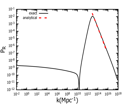
Figure 2: The power spectrum (left) with solid line (numerical) and with dashed (analytical from Eq. 2.34). The density of stochastic GWs (right). Both plots are for the case of modifying Wess-Zumino superpotential. We choose $\lambda/\mu=1/3$, $c_{1}=1.9$, $c_{2}=-0.73$ and $b_{1}=3.9615$.

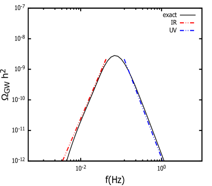
Figure 3: The energy density of GWs for the case of modifying Wess-Zumino superpotential. Dashed lines corresponds to analytical approximation of the IR slope (red) and UV slope (blue).

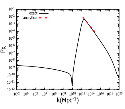
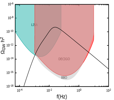
Figure 4: The power spectrum (left) with solid line (numerical) and with dashed (analytical from Eq. 2.34). The density of stochastic GW (right). Both plots are for the case of modifying Cecotti superpotential. We choose $c_{3}=13.2$, $l=1.00028$ and $b_{2}=8.575$.

4.2 Modifying the Kähler potential

In this section we present the results of the power spectrum and the abundances of GWs in the case of the modified Kähler potential, given in Eqs. (3.9) and (3.11). This case is more labored than the previous one, because there is analytic expression for transformation of the field, in order to have canonical kinetic terms. Hence, the Eq. (2.19) should be used. We proceed with the numerical integration of background and curvature perturbations of the field, assuming that we are in Bunch-Davies vacuum, given in Eqs. (2.24), (2.26) and (2.27), as we have discussed before.

In Figs. 5 and 6 we present the resulting power spectrum and the density abundance of GWs for the Eqs. (3.9) and (3.11), respectively. The choice of initial conditions and the prediction for $n_{s}$ and $r$ are given in Table 2. In this table we present the initial condition for the canonical normalized field, which we denote with $\phi$. In this Table we show that the prediction of $n_{s}$ and $r$ are consistent with the Planck constraints[62, 63], as in the previous cases.

	$\phi_{ic}$	$n_{s}$	$r$
1	$4.899$	$0.9612$	$0.0121$
2	$4.097$	$0.9601$	$0.0092$

Table 2: Initial conditions for the field for the Eqs. (3.7) and (3.9) and the prediction of $n_{s}$ and $r$.

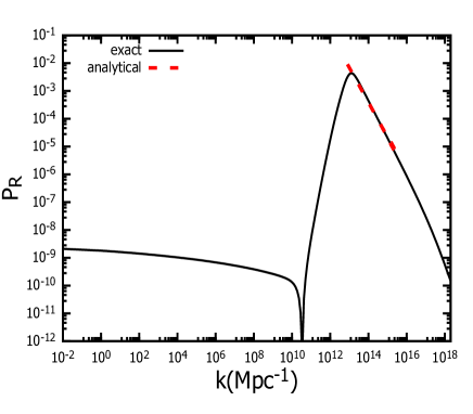
Figure 5: The power spectrum (left) with solid line (numerical) and with dashed (analytical from Eq. 2.34). The density of stochastic GWs (right) for the case of modifying Wess-Zumino. We choose for the parameters $b_{3}=87.38$, $c=0.065$, $c_{3}=-4$ and $\lambda/\mu=0.33327$

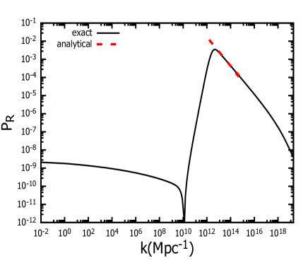
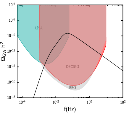
Figure 6: The power spectrum (left) with solid line (numerical) and with dashed (analytical from Eq. 2.34). The density of stochastic GWs (right) for the case of modifying Cecotti. The parameters are $d=-0.054$, $b_{4}=7.51511$, $c_{4}=8.8$, $\bar{\lambda}=-0.5$ and $\bar{\mu}=1.0$

In left panels in the Figs. 5 and 6 we also show the numerical and analytical results of power spectrum from Eqs. (2.33) and (2.34). The value of $n$ in Eq. (2.34) ranges from $0.15$ to $2.7$ [75]. In both models, either by modifying the Kähler potential or by modifying the superpotential), $n$ ranges from 0.8 to 1.8. Hence, in order to estimate the effect of the non-gaussianities the analysis of [75] can be used. In particular, this related to the peaks of power spectrum $P_{peak}=10^{-3}-10^{-2}$ as $f_{NL}\lessapprox 10^{-2}$. Generally, the amplitude $f_{NL}$ is defined as

$$f_{NL}=\frac{5}{6}\frac{\mathcal{B}(k_{1},k_{2},k_{3})}{P_{R}(k_{1})P_{R}(k_{2})+P_{R}(k_{1})P_{R}(k_{3})+P_{R}(k_{2})P_{R}(k_{3})}\,,$$ (4.14)

where $\mathcal{B}$ is the bispectrum. According to the study [75] the non-gausianities of models with an enhanced power spectrum can be large enough not to satisfy the constraints on the PBHs abundance. We note that in this paper we focus in the production of GWs, as the production of the PBHs for these models has already presented elsewhere [21, 22].

The production of PBHs using similar modifications in the SUGRA model has been studied in [22]. There, it was concluded that the maximum value of the peak of the power spectrum should be around $3-5\times 10^{-2}$. In this analysis here, that refers to the production of GWs this restriction does not apply.

That is, the power spectra of GWs, will be detected by future experiments, such as LISA or DECIGO even if the high of the peak of the power spectrum is smaller than $10^{-2}$. On the other hand, the abundance of the PBHs is exponentially sensitive to the mass fraction of the Universe that collapse to PBHs  [84, 85, 86, 87, 88]. Consequently, it is expected that the amount of the fine-tuning in the parameters of the extra terms, will be reduced. We discuss this point in Appendix B.

5 Conclusions

In this paper we introduce four models in order to propose a possible scenario for the production of GWs, that can be detected by future space-based experiments of GWs. A well-known way to get amplified production of the GWs is an enhancement in the scalar power spectrum, since the first and second order spectra are related. There are many mechanisms proposed in the literature, in order to get such an enhancement. In our study we employed this of the near inflection point, in the context of single field inflation. We embedded this scenario in models derived by no-scale SUGRA theory and especially we consider models that conserve and break the SU(2,1)/SU(2)$\times$ U(1) symmetry.

First, we modified the Wess-Zumino and the Cecotti superpotentials. These modifications leads to the effective scalar potential, which is equivalent in both bases $(T,\varphi)$ and $(y_{1},y_{2})$. Both of these models can conserve the SU(2,1)/SU(2)$\times$ U(1) symmetry, as we can properly interplay between the fields $y_{1}$ and $y_{2}$ and we can derive the same effective scalar potential. The same potential can be found, if we transform the fields and use the equivalent forms in the $(T,\varphi)$ basis. The equivalence between the models has been studied for the unmodified case. However, in our study we have the additional feature of an inflection point that leads to a significant enhancement of the scalar power spectrum.

Secondly, we keep these two superpotentials, Wess-Zumino and Cecotti, unchanged and we modify the Kähler potential in $(T,\varphi)$ basis. The resulting effective scalar potential can only be given numerically, as there is not an analytical solution with canonical kinetic term. Hence, we derive four inflationary potentials with a near inflection point.

This enhancement of scalar power spectrum is expected to be imprinted in the energy density of GWs. In order to evaluate this energy density, we calculate numerically the perturbations of the field for all the proposed potentials. We evaluate the scalar power spectrum and then the corresponding energy densities of GWs. We show that these models give sizable GWs spectra, which can be detected by the future experiments. Last but not least, all the models presented in this work are consistent with the observational constraints on inflation.

Appendix A The forms of the scalar potential

In general the scalar potential can be evaluated in the framework of supergravity, if we use the following expression:

$$V=e^{K}(D_{\Phi}WK^{\bar{\Phi}\Phi}D_{\bar{\Phi}}\bar{W}-3|W|^{2})\,,$$ (A.1)

where

$$D_{\Phi}W=\frac{\partial W}{\partial\Phi}+\frac{\partial K}{\partial\Phi}W.$$ (A.2)

In this Appendix we sum up the four models proposed in the text and we present the effective scalar potentials for the two first models.

A.1 Model I

For the choice of Kähler potential

$$K=-3\ln(1-\frac{|y_{1}|^{2}}{3}-\frac{|y_{2}|^{2}}{3})$$ (A.3)

we modify the superpotential given in Eq. (2.12) as:

$$W=\left[\frac{\hat{\mu}}{2}\left(y_{1}^{2}+\frac{y_{2}^{2}y_{1}}{\sqrt{3}}\right)-\lambda\frac{y_{1}^{3}}{3}\right]\left[1+e^{-b_{1}y_{1}^{2}}\left(c_{1}{y_{1}}^{2}+c_{2}{y_{1}}^{4}\right)\right]\,$$ (A.4)

where $\hat{\mu}$, $\lambda$, $b_{1}$, $c_{1}$ and $c_{2}$ are free parameters. If we use Eq. (A.1), the effective scalar potential becomes:

$$\begin{split}V/\mu^{2}&=\sinh^{2}\left(\frac{\phi}{\sqrt{6}}\right)\Big{[}9\tanh^{4}\left(\frac{\phi}{\sqrt{6}}\right)e^{-6b_{1}\tanh^{2}\left(\frac{\phi}{\sqrt{6}}\right)}\left(\mu-2\lambda\tanh\left(\frac{\phi}{\sqrt{6}}\right)\right)^{2}\times\\ &\times\left(\tanh^{2}\left(\frac{\phi}{\sqrt{6}}\right)(6{c_{2}}-3b_{1}c_{1})-9b_{1}{c_{2}}\tanh^{4}\left(\frac{\phi}{\sqrt{6}}\right)+c_{1}\right)^{2}-\\ &-3\sinh^{2}\left(\frac{\phi}{\sqrt{6}}\right)e^{-6b_{1}\tanh^{2}\left(\frac{\phi}{\sqrt{6}}\right)}\left(\mu-2\lambda\tanh\left(\frac{\phi}{\sqrt{6}}\right)\right)\times\\ &\times\left(2\mu-6\lambda\tanh\left(\frac{\phi}{\sqrt{6}}\right)+\mu\tanh^{2}\left(\frac{\phi}{\sqrt{6}}\right)\right)\cosh^{2}\left(\frac{\phi}{\sqrt{6}}\right)\left(\mu-3\lambda\tanh\left(\frac{\phi}{\sqrt{6}}\right)\right)^{2}\\ &\times\left(3\tanh^{2}\left(\frac{\phi}{\sqrt{6}}\right)e^{-3b_{1}\tanh^{2}\left(\frac{\phi}{\sqrt{6}}\right)}\left(c_{1}+3{c_{2}}\tanh^{2}\left(\frac{\phi}{\sqrt{6}}\right)\right)+1\right)^{2}+\\ &+\left(e^{3b_{1}\tanh^{2}\left(\frac{\phi}{\sqrt{6}}\right)}+3c_{1}\tanh^{2}\left(\frac{\phi}{\sqrt{6}}\right)+9{c_{2}}\tanh^{4}\left(\frac{\phi}{\sqrt{6}}\right)\right)\times\\ &\times\left(3\tanh^{2}\left(\frac{\phi}{\sqrt{6}}\right)(b_{1}c_{1}-2{c_{2}})+9b_{1}{c_{2}}\tanh^{4}\left(\frac{\phi}{\sqrt{6}}\right)-c_{1}\right)\Big{]}\end{split}$$ (A.5)

where $\hat{\mu}=\mu\sqrt{c/3}$. We have considered that the inflationary direction for this example is given as:

$$y_{1}=\varphi,\quad y_{2}=0.$$ (A.6)

Moreover, in order to have fix the non- canonical kinetic term we consider the redefinition of the field:

$$y_{1}=-\sqrt{3}\tanh\left(\frac{\phi}{\sqrt{6}}\right)\,.$$ (A.7)

We remark that the same effective scalar potential can be derived if we have the following transformations: $y_{1}\rightarrow-y_{1}$ and $y_{2}\rightarrow-y_{2}$ [22, 64].

The same form of the potential can be derived, if we use the basis $(T,\varphi)$ with the tranformation described in the text from Eqs.(2.8), (2.9) and (2.10). Hence, we have the following forms:

$$K=-3\ln(T+\bar{T}-\frac{|\varphi|^{2}}{3})$$ (A.8)

$$W=\left(\frac{\hat{\mu}}{2}\varphi^{2}-\frac{\lambda}{3}\varphi^{3}\right)\left(1+e^{-b_{1}\left(\frac{2\varphi}{1+2T}\right)^{2}}\left[c_{1}\left(\frac{2\varphi}{1+2T}\right)^{2}+c_{2}\left(\frac{2\varphi}{1+2T}\right)^{4}\right]\right).$$ (A.9)

We choose the following direction $T=Im\varphi=0$ and $Re\varphi=\phi$ and we apply Eq. (A.1).

A.2 Model II

For the choice of Kähler potential (A.3) we modify the superpotential given in Eq. (2.17) as:

$$W=m\left(-y_{1}y_{2}+\frac{y_{2}y_{1}^{2}}{l\sqrt{3}}\right)\left(1+c_{3}e^{-b_{2}{y_{1}}^{2}}{y_{1}}^{2}\right)\,.$$ (A.10)

From Eq. (A.1) we derive the form of effective scalar potential, which is given as follows:

$$\begin{split}V/m^{2}&=\frac{3}{l^{2}}\sinh^{2}\left(\frac{\phi}{\sqrt{6}}\right)\cosh^{2}\left(\frac{\phi}{\sqrt{6}}\right)e^{-6b\tanh^{2}\left(\frac{\phi}{\sqrt{6}}\right)}\left(l-\tanh\left(\frac{\phi}{\sqrt{6}}\right)\right)^{2}\\ &\times\left(e^{3b\tanh^{2}\left(\frac{\phi}{\sqrt{6}}\right)}+3c_{3}\tanh^{2}\left(\frac{\phi}{\sqrt{6}}\right)\right)^{2}.\end{split}$$ (A.11)

As in model 1, we choose the inflationary direction (A.6) and we fix the non- canonical kinetic terms. This potential has the following free parameters: $l$, $b_{2}$ and $c_{3}$.

We can use the other form of the Kähler potential (A.8) and with proper tranformations given from Eqs.(2.8), (2.9) and (2.10) we can take the equivalent form of the superpotential in the basis $(T,\varphi)$. The superpotential is given as follows:

$$W=\frac{\sqrt{3}}{2}m\varphi\Big{(}\frac{1}{2}-T\Big{)}\left(-1-2T-\frac{1-2T}{l}\right)\left[1+3c_{3}e^{-3b_{2}\left(\frac{1-2T}{1+2T}\right)^{2}}\left(\frac{1-2T}{1+2T}\right)^{2}\right]\,.$$ (A.12)

A.3 Model III

In this model we do not change the superpotential but the Kähler potential in $(T,\varphi)$ basis. For superpotential we choose this of Wess Zumino model described in Eq. (2.12).

$$K=-3\ln(T+\bar{T}-\frac{\varphi\bar{\varphi}}{3}+c_{4}e^{-b_{3}(\varphi+\bar{\varphi})^{2}}(\varphi+\bar{\varphi})^{4})\,,$$ (A.13)

$$W=\frac{\hat{\mu}}{2}\varphi^{2}-\frac{\lambda}{3}\varphi^{3}.$$ (A.14)

We can evaluate the scalar potential from (A.1). In this case the non-canonical kinetic term can be fixed only numerically. The direction of inflation is $T=c/2$ and $\varphi=\phi$. The free parameters for this case are $c$, $\lambda$, $\mu$, $c_{3}$, $b_{3}$ and $c$.

A.4 Model IV

In this model we modify the described in Eq.(A.8) and we keep unchanged the Cecotti superpotential given in (2.17). Hence we have:

$$K=-3\ln(T+\bar{T}-\frac{\varphi\bar{\varphi}}{3}+F(T+\bar{T},\varphi+\bar{\varphi}))$$ (A.15)

$$W=\sqrt{3}m\varphi\left(T-\frac{1}{2}\right)$$ (A.16)

where $F(T+\bar{T},\varphi+\bar{\varphi})$ is a function of both chiral fields. We choose the following form

$$F(T+\bar{T},\varphi+\bar{\varphi})=e^{-d(T+\bar{T})}\left(c_{4}e^{-b_{4}(T+\bar{T})}(T+\bar{T})^{2}+\bar{\lambda}(\varphi+\bar{\varphi}+\bar{\mu})\right)\,,$$ (A.17)

and we assume that the inflationary direction is

$$T=ReT=\phi,\quad ImT=\varphi=0.$$ (A.18)

The scalar power spectrum can be evaluated numerically by using Eq. (A.1). We need to consider the transformation of the field in order to have canonical kinetic term. This redefinition can be evaluated only numerically as in the previous case. The free parameters are $m$, $d$, $b_{4}$, $c_{4}$, $\bar{\lambda}$ and $\bar{\mu}$.

Appendix B Fine-tuning analysis and a comparison between the models

It is well-known that the enhancement of scalar power spectrum, which occurs due to the inflection point in the effective scalar potential requires a lot of fine-tuning [19]. The value of this enhancement can be smaller in the case of studying the production of GWs than in the case of studying the amount of DM from the PBHs. In Ref. [22] there is a discussion explaining how the parameters of the potential presented in this work arise. In this Appendix we analyse the level of fine-tuning by considering the parameter $b_{i}$, which is presented throughout this work and is the parameter, which depends on the power spectrum’s peak and demands more fine-tuning.

The role of the parameter $b_{i}$ is to trigger an enhancement in the power spectrum. In order to analyze the level of fine-tuning, we calculate the parameter $\Delta_{b}$, which is shown in Refs. [89, 90] and it is given as the max value of the follow quantity

$$\Delta_{b}=\left|\frac{\partial\ln(P_{R}^{peak})}{\partial\ln(b_{i})}\right|\,.$$ (B.1)

In the following, we study the fine-tuning of the function $P_{R}^{peak}(b_{i})$. Large value of the maximum of the quantity $\Delta_{b}$ means that a high level of fine-tuning is required. As we mentioned before, we expect that the fine-tuning of the parameters can be decreased in the study of generation of GWs, due to its wider range of peak’s height in comparison with the production of PBHs.

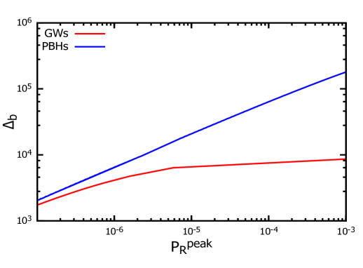
Figure 7: The level of fine-tuning for the case (3.7).

In Fig.7 we show the quantity $\Delta_{b}$ as a function of the peak of the power spectrum. In particular we show how the quantity $\Delta_{b}$ varies in respect to the values of the spectrum’s peak in the case of study PBHs (blue line) and in the case of GWs (red line). The case for this plot is the model described from the Eqs.(3.7) and( 3.8) (model III of Appendix A). As one can notice we need more fine-tuning when we study PBHs. This occurs not only due to smaller peaks, which are needed in the study of GWs, but also due to the specific value of the threshold presented in the evaluation of the production of PBHs. Specifically, in order to obtain a significant amount of DM from PBHs and to use the proposed values for threshold, as analysed in [84, 85, 86, 87, 88], we need to properly adjust the extra parameters of the model. This increases the fine-tuning in the study of PBHs.

We remark that in the previous study of Refs [22], where the fine-tuning for the PBHs production is analysed, the maximum value of $(\Delta_{b})$ was at the order of magnitude of $10^{6}$. In a relevant study of Ref.  [19] the amount of fine-tuning for PBHs was at level of $10^{8}$. It is possible that the fine-tuning can be decreased further. In Table 3, we show the value of the maximum of $\Delta_{b}$, assuming that we have the minimal enhancement of peak of the power spectrum, in order to predict the future space based experiment DECIGO. In other words, we calculate the max( $\Delta_{b}$) by considering that the peak of power spectrum is around $k=10^{-5}$. In Table 3 we present, for comparison, the maximum value of $\Delta_{b}$ for PBHs, as adopted in Refs. [21, 22]. One can notice that there is sizable difference with respect to the case of the production of the GWs. Specifically, the fine-tuning in our current analysis is smaller at least two orders of magnitude.

case	max$(\Delta_{b})_{PBHs}$	max$(\Delta_{b})_{GWs}$
1	$7.9$ $\times 10^{5}$	$3.5$ $\times 10^{3}$
2	$9.8$ $\times 10^{5}$	$3.6$ $\times 10^{3}$
3	$1.6$ $\times 10^{5}$	$8.5\times 10^{2}$
4	$4.2$ $\times 10^{6}$	$5.6$ $\times 10^{4}$

Table 3: The maximum value for $\Delta_{b}$ for the cases in Eqs. (3.2), (3.5),(3.7) and (3.9) respectively. The abundances of PBHs are adopted by [21, 22]. Details given are in main text.

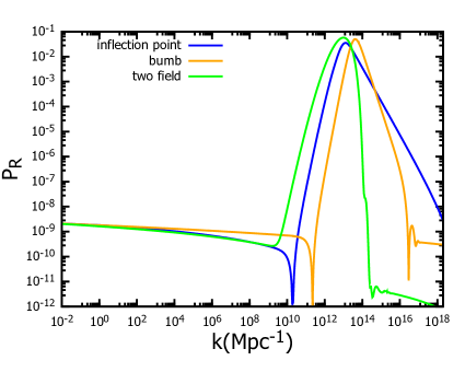
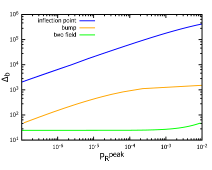
Figure 8: The level of fine-tuning for our model (blue) with comparison with this amount from other models.

Finally, in order to have a comparison with the previous mechanisms with an enhancement in scalar power spectrum analysed in the literature, we depict the quantity $\Delta_{b}$ for different models. In particular, in Fig.8 we show the power spectrum for the case given Eqs.(3.7) and( 3.8) with blue lines. Orange lines corresponds to the model presented in [77] where the enhancement of power spectrum comes from a bulky potential. Green lines to the two- model shown in [24]. In this work a two field model with a non-canonical kinetic term has been proposed. In both these models the underlying parameter b needs fine-tuning in order to obtain the proper enhancement. The left panel of the Fig.8 shows the power spectrum of these models, reproduced by the methodology of subsection 2.2 and the right panel shows the quantity $\Delta_{b}$. We notice that models with an inflection point have more fine-tuning than the other ones. Models with a bumb feature in the potential have significantly less fine-tuning than the models with an inflection point. Finally, models with two fields experience the less fine-tuning of all cases.

References

- [1] B. P. Abbott, et al., Observation of Gravitational Waves from a Binary Black Hole Merger, Phys. Rev. Lett. 116 (6) (2016) 061102. arXiv:1602.03837, doi:10.1103/PhysRevLett.116.061102.
- [2] B. P. Abbott, et al., GW170104: Observation of a 50-Solar-Mass Binary Black Hole Coalescence at Redshift 0.2, Phys. Rev. Lett. 118 (22) (2017) 221101, [Erratum: Phys.Rev.Lett. 121, 129901 (2018)]. arXiv:1706.01812, doi:10.1103/PhysRevLett.118.221101.
- [3] B. P. Abbott, et al., GW170608: Observation of a 19-solar-mass Binary Black Hole Coalescence, Astrophys. J. Lett. 851 (2017) L35. arXiv:1711.05578, doi:10.3847/2041-8213/aa9f0c.
- [4] B. P. Abbott, et al., GW170814: A Three-Detector Observation of Gravitational Waves from a Binary Black Hole Coalescence, Phys. Rev. Lett. 119 (14) (2017) 141101. arXiv:1709.09660, doi:10.1103/PhysRevLett.119.141101.
- [5] B. P. Abbott, et al., GW151226: Observation of Gravitational Waves from a 22-Solar-Mass Binary Black Hole Coalescence, Phys. Rev. Lett. 116 (24) (2016) 241103. arXiv:1606.04855, doi:10.1103/PhysRevLett.116.241103.
- [6] P. Amaro-Seoane, et al., Laser Interferometer Space Antenna (2 2017). arXiv:1702.00786.
- [7] K. Yagi, N. Seto, Detector configuration of DECIGO/BBO and identification of cosmological neutron-star binaries, Phys. Rev. D 83 (2011) 044011, [Erratum: Phys.Rev.D 95, 109901 (2017)]. arXiv:1101.3940, doi:10.1103/PhysRevD.83.044011.
-
[8]
S. Hawking, Gravitationally
Collapsed Objects of Very Low Mass, Monthly Notices of the Royal
Astronomical Society 152 (1) (1971) 75–78.
arXiv:https://academic.oup.com/mnras/article-pdf/152/1/75/9360899/mnras152-0075.pdf,
doi:10.1093/mnras/152.1.75.
URL https://doi.org/10.1093/mnras/152.1.75 - [9] S. W. Hawking, Gravitational radiation from colliding black holes, Phys. Rev. Lett. 26 (1971) 1344–1346. doi:10.1103/PhysRevLett.26.1344.
- [10] B. J. Carr, S. W. Hawking, Black holes in the early Universe, Mon. Not. Roy. Astron. Soc. 168 (1974) 399–415.
- [11] Y. B. Zel’dovich, I. D. Novikov, The Hypothesis of Cores Retarded during Expansion and the Hot Cosmological Model, Soviet Astron. AJ (Engl. Transl. ), 10 (1967) 602.
- [12] M. Sasaki, T. Suyama, T. Tanaka, S. Yokoyama, Primordial black holes—perspectives in gravitational wave astronomy, Class. Quant. Grav. 35 (6) (2018) 063001. arXiv:1801.05235, doi:10.1088/1361-6382/aaa7b4.
- [13] J. Garcia-Bellido, E. Ruiz Morales, Primordial black holes from single field models of inflation, Phys. Dark Univ. 18 (2017) 47–54. arXiv:1702.03901, doi:10.1016/j.dark.2017.09.007.
- [14] G. Ballesteros, M. Taoso, Primordial black hole dark matter from single field inflation, Physical Review D 97 (2) (jan 2018). doi:10.1103/physrevd.97.023501.
- [15] O. Özsoy, S. Parameswaran, G. Tasinato, I. Zavala, Mechanisms for primordial black hole production in string theory, Journal of Cosmology and Astroparticle Physics 2018 (07) (2018) 005–005. doi:10.1088/1475-7516/2018/07/005.
- [16] M. Cicoli, V. A. Diaz, F. G. Pedro, Primordial black holes from string inflation, Journal of Cosmology and Astroparticle Physics 2018 (06) (2018) 034–034. doi:10.1088/1475-7516/2018/06/034.
- [17] T.-J. Gao, Z.-K. Guo, Primordial Black Hole Production in Inflationary Models of Supergravity with a Single Chiral Superfield, Phys. Rev. D 98 (6) (2018) 063526. arXiv:1806.09320, doi:10.1103/PhysRevD.98.063526.
- [18] I. Dalianis, A. Kehagias, G. Tringas, Primordial black holes from -attractors, JCAP 01 (2019) 037. arXiv:1805.09483, doi:10.1088/1475-7516/2019/01/037.
- [19] M. P. Hertzberg, M. Yamada, Primordial Black Holes from Polynomial Potentials in Single Field Inflation, Phys. Rev. D 97 (8) (2018) 083509. arXiv:1712.09750, doi:10.1103/PhysRevD.97.083509.
- [20] R. Mahbub, Primordial black hole formation in inflationary -attractor models, Phys. Rev. D 101 (2) (2020) 023533. arXiv:1910.10602, doi:10.1103/PhysRevD.101.023533.
- [21] D. V. Nanopoulos, V. C. Spanos, I. D. Stamou, Primordial Black Holes from No-Scale Supergravity, Phys. Rev. D 102 (8) (2020) 083536. arXiv:2008.01457, doi:10.1103/PhysRevD.102.083536.
- [22] I. D. Stamou, Mechanisms of Producing Primordial Black Holes By Breaking The SU(2,1)/SU(2)U(1) Symmetry, Phys. Rev. D 103 (8) (2021) 083512. arXiv:2104.08654, doi:10.1103/PhysRevD.103.083512.
- [23] J. M. Ezquiaga, J. Garcia-Bellido, E. Ruiz Morales, Primordial Black Hole production in Critical Higgs Inflation, Phys. Lett. B 776 345–349. arXiv:1705.04861, doi:10.1016/j.physletb.2017.11.039.
- [24] M. Braglia, D. K. Hazra, F. Finelli, G. F. Smoot, L. Sriramkumar, A. A. Starobinsky, Generating PBHs and small-scale GWs in two-field models of inflation, JCAP 08 (2020) 001. arXiv:2005.02895, doi:10.1088/1475-7516/2020/08/001.
- [25] M. Braglia, X. Chen, D. K. Hazra, Probing Primordial Features with the Stochastic Gravitational Wave Background, JCAP 03 (2021) 005. arXiv:2012.05821, doi:10.1088/1475-7516/2021/03/005.
- [26] Y. Aldabergenov, A. Addazi, S. V. Ketov, Primordial black holes from modified supergravity, Eur. Phys. J. C 80 (10) (2020) 917. arXiv:2006.16641, doi:10.1140/epjc/s10052-020-08506-6.
- [27] Y. Aldabergenov, A. Addazi, S. V. Ketov, Testing Primordial Black Holes as Dark Matter in Supergravity from Gravitational Waves, Phys. Lett. B 814 (2021) 136069. arXiv:2008.10476, doi:10.1016/j.physletb.2021.136069.
-
[28]
K. Tomita, Non-Linear Theory of
Gravitational Instability in the Expanding Universe, Progress of
Theoretical Physics 37 (5) (1967) 831–846.
arXiv:https://academic.oup.com/ptp/article-pdf/37/5/831/5234391/37-5-831.pdf,
doi:10.1143/PTP.37.831.
URL https://doi.org/10.1143/PTP.37.831 -
[29]
S. Matarrese, O. Pantano, D. Saez,
General-relativistic
approach to the nonlinear evolution of collisionless matter, Phys. Rev. D 47
(1993) 1311–1323.
doi:10.1103/PhysRevD.47.1311.
URL https://link.aps.org/doi/10.1103/PhysRevD.47.1311 - [30] V. Acquaviva, N. Bartolo, S. Matarrese, A. Riotto, Second order cosmological perturbations from inflation, Nucl. Phys. B 667 (2003) 119–148. arXiv:astro-ph/0209156, doi:10.1016/S0550-3213(03)00550-9.
- [31] K. N. Ananda, C. Clarkson, D. Wands, The Cosmological gravitational wave background from primordial density perturbations, Phys. Rev. D 75 (2007) 123518. arXiv:gr-qc/0612013, doi:10.1103/PhysRevD.75.123518.
- [32] D. Baumann, P. J. Steinhardt, K. Takahashi, K. Ichiki, Gravitational Wave Spectrum Induced by Primordial Scalar Perturbations, Phys. Rev. D 76 (2007) 084019. arXiv:hep-th/0703290, doi:10.1103/PhysRevD.76.084019.
- [33] J. R. Espinosa, D. Racco, A. Riotto, A Cosmological Signature of the SM Higgs Instability: Gravitational Waves, JCAP 09 (2018) 012. arXiv:1804.07732, doi:10.1088/1475-7516/2018/09/012.
- [34] K. Inomata, K. Kohri, T. Nakama, T. Terada, Enhancement of Gravitational Waves Induced by Scalar Perturbations due to a Sudden Transition from an Early Matter Era to the Radiation Era, Phys. Rev. D 100 (4) (2019) 043532. arXiv:1904.12879, doi:10.1103/PhysRevD.100.043532.
- [35] J. Adams, B. Cresswell, R. Easther, Inflationary perturbations from a potential with a step, Physical Review D 64 (12) (nov 2001). doi:10.1103/physrevd.64.123514.
- [36] K. Kefala, G. P. Kodaxis, I. D. Stamou, N. Tetradis, Features of the inflaton potential and the power spectrum of cosmological perturbations (10 2020). arXiv:2010.12483.
- [37] I. Dalianis, G. P. Kodaxis, I. D. Stamou, N. Tetradis, A. Tsigkas-Kouvelis, Spectrum oscillations from features in the potential of single-field inflation, Phys. Rev. D 104 (10) (2021) 103510. arXiv:2106.02467, doi:10.1103/PhysRevD.104.103510.
- [38] Y.-F. Cai, X.-H. Ma, M. Sasaki, D.-G. Wang, Z. Zhou, One small step for an inflaton, one giant leap for inflation: A novel non-Gaussian tail and primordial black holes, Phys. Lett. B 834 (2022) 137461. arXiv:2112.13836, doi:10.1016/j.physletb.2022.137461.
- [39] C. Pattison, V. Vennin, D. Wands, H. Assadullahi, Ultra-slow-roll inflation with quantum diffusion, JCAP 04 (2021) 080. arXiv:2101.05741, doi:10.1088/1475-7516/2021/04/080.
- [40] C. T. Byrnes, P. S. Cole, S. P. Patil, Steepest growth of the power spectrum and primordial black holes, JCAP 06 (2019) 028. arXiv:1811.11158, doi:10.1088/1475-7516/2019/06/028.
- [41] S. Clesse, J. García-Bellido, Massive Primordial Black Holes from Hybrid Inflation as Dark Matter and the seeds of Galaxies, Phys. Rev. D 92 (2) (2015) 023524. arXiv:1501.07565, doi:10.1103/PhysRevD.92.023524.
- [42] V. C. Spanos, I. D. Stamou, Gravitational waves and primordial black holes from supersymmetric hybrid inflation, Phys. Rev. D 104 (12) (2021) 123537. arXiv:2108.05671, doi:10.1103/PhysRevD.104.123537.
- [43] A. Gundhi, S. V. Ketov, C. F. Steinwachs, Primordial black hole dark matter in dilaton-extended two-field Starobinsky inflation, Phys. Rev. D 103 (8) (2021) 083518. arXiv:2011.05999, doi:10.1103/PhysRevD.103.083518.
- [44] S. Pi, M. Sasaki, Primordial Black Hole Formation in Non-Minimal Curvaton Scenario (12 2021). arXiv:2112.12680.
- [45] G. Domènech, Scalar Induced Gravitational Waves Review, Universe 7 (11) (2021) 398. arXiv:2109.01398, doi:10.3390/universe7110398.
- [46] G. Domènech, Induced gravitational waves in a general cosmological background, Int. J. Mod. Phys. D 29 (03) (2020) 2050028. arXiv:1912.05583, doi:10.1142/S0218271820500285.
- [47] G. Domènech, S. Pi, M. Sasaki, Induced gravitational waves as a probe of thermal history of the universe, JCAP 08 (2020) 017. arXiv:2005.12314, doi:10.1088/1475-7516/2020/08/017.
- [48] Z. Zhou, J. Jiang, Y.-F. Cai, M. Sasaki, S. Pi, Primordial black holes and gravitational waves from resonant amplification during inflation, Phys. Rev. D 102 (10) (2020) 103527. arXiv:2010.03537, doi:10.1103/PhysRevD.102.103527.
- [49] J. Fumagalli, S. Renaux-Petel, L. T. Witkowski, Oscillations in the stochastic gravitational wave background from sharp features and particle production during inflation (12 2020). arXiv:2012.02761.
- [50] I. Dalianis, K. Kritos, Exploring the Spectral Shape of Gravitational Waves Induced by Primordial Scalar Perturbations and Connection with the Primordial Black Hole Scenarios, Phys. Rev. D 103 (2) (2021) 023505. arXiv:2007.07915, doi:10.1103/PhysRevD.103.023505.
- [51] G. Domènech, C. Lin, M. Sasaki, Gravitational wave constraints on the primordial black hole dominated early universe, JCAP 04 (2021) 062. arXiv:2012.08151, doi:10.1088/1475-7516/2021/04/062.
- [52] G. Domènech, M. Sasaki, Approximate gauge independence of the induced gravitational wave spectrum, Phys. Rev. D 103 (6) (2021) 063531. arXiv:2012.14016, doi:10.1103/PhysRevD.103.063531.
- [53] I. Dalianis, C. Kouvaris, Gravitational Waves from Density Perturbations in an Early Matter Domination Era (12 2020). arXiv:2012.09255.
- [54] W.-T. Xu, J. Liu, T.-J. Gao, Z.-K. Guo, Gravitational waves from double-inflection-point inflation, Phys. Rev. D 101 (2) (2020) 023505. arXiv:1907.05213, doi:10.1103/PhysRevD.101.023505.
- [55] T.-J. Gao, X.-Y. Yang, Double peaks of gravitational wave spectrum induced from inflection point inflation (1 2021). arXiv:2101.07616.
- [56] G. Ballesteros, J. Rey, M. Taoso, A. Urbano, Primordial black holes as dark matter and gravitational waves from single-field polynomial inflation, JCAP 07 (2020) 025. arXiv:2001.08220, doi:10.1088/1475-7516/2020/07/025.
- [57] E. Cremmer, S. Ferrara, C. Kounnas, D. V. Nanopoulos, Naturally Vanishing Cosmological Constant in N=1 Supergravity, Phys. Lett. B 133 (1983) 61. doi:10.1016/0370-2693(83)90106-5.
- [58] J. R. Ellis, A. B. Lahanas, D. V. Nanopoulos, K. Tamvakis, No-Scale Supersymmetric Standard Model, Phys. Lett. B 134 (1984) 429. doi:10.1016/0370-2693(84)91378-9.
- [59] J. R. Ellis, C. Kounnas, D. V. Nanopoulos, Phenomenological SU(1,1) Supergravity, Nucl. Phys. B 241 (1984) 406–428. doi:10.1016/0550-3213(84)90054-3.
- [60] J. R. Ellis, C. Kounnas, D. V. Nanopoulos, No Scale Supersymmetric Guts, Nucl. Phys. B 247 (1984) 373–395. doi:10.1016/0550-3213(84)90555-8.
- [61] A. B. Lahanas, D. V. Nanopoulos, The Road to No Scale Supergravity, Phys. Rept. 145 (1987) 1. doi:10.1016/0370-1573(87)90034-2.
- [62] B. A. et al. (LIGO Scientific Collaboration, V. Collaboration), Planck2015 results, Astronomy & Astrophysics 594 (2016) A20. doi:10.1051/0004-6361/201525898.
- [63] Y. A. et. al. [Planck Collaboration], Planck 2018 results. x. constraints on inflationarXiv:http://arxiv.org/abs/1807.06211v2.
- [64] J. Ellis, D. V. Nanopoulos, K. A. Olive, S. Verner, A general classification of Starobinsky-like inflationary avatars of SU(2,1)/SU(2) U(1) no-scale supergravity, JHEP 03 (2019) 099. arXiv:1812.02192, doi:10.1007/JHEP03(2019)099.
- [65] J. Ellis, D. V. Nanopoulos, K. A. Olive, Starobinsky-like Inflationary Models as Avatars of No-Scale Supergravity, JCAP 10 (2013) 009. arXiv:1307.3537, doi:10.1088/1475-7516/2013/10/009.
- [66] S. Cecotti, Higher Derivative Supergravity Is Equivalent To Standard Supergravity Coupled To Matter. 1., Phys. Lett. B 190 (1987) 86–92. doi:10.1016/0370-2693(87)90844-6.
- [67] J. Ellis, D. V. Nanopoulos, K. A. Olive, No-Scale Supergravity Realization of the Starobinsky Model of Inflation, Phys. Rev. Lett. 111 (2013) 111301, [Erratum: Phys.Rev.Lett. 111, 129902 (2013)]. arXiv:1305.1247, doi:10.1103/PhysRevLett.111.111301.
- [68] R. Kallosh, A. Linde, Universality Class in Conformal Inflation, JCAP 07 (2013) 002. arXiv:1306.5220, doi:10.1088/1475-7516/2013/07/002.
- [69] S. Ferrara, R. Kallosh, A. Linde, M. Porrati, Minimal Supergravity Models of Inflation, Phys. Rev. D 88 (8) (2013) 085038. arXiv:1307.7696, doi:10.1103/PhysRevD.88.085038.
- [70] R. Kallosh, A. Linde, D. Roest, Large field inflation and double -attractors, JHEP 08 (2014) 052. arXiv:1405.3646, doi:10.1007/JHEP08(2014)052.
-
[71]
V. Mukhanov, H. Feldman, R. Brandenberger,
Theory
of cosmological perturbations, Physics Reports 215 (5) (1992) 203–333.
doi:https://doi.org/10.1016/0370-1573(92)90044-Z.
URL https://www.sciencedirect.com/science/article/pii/037015739290044Z - [72] V. F. Mukhanov, Quantum Theory of Gauge Invariant Cosmological Perturbations, Sov. Phys. JETP 67 (1988) 1297–1302.
- [73] C. Ringeval, The exact numerical treatment of inflationary models, Lect. Notes Phys. 738 (2008) 243–273. arXiv:astro-ph/0703486, doi:10.1007/978-3-540-74353-8_7.
- [74] K. Kohri, T. Terada, Semianalytic calculation of gravitational wave spectrum nonlinearly induced from primordial curvature perturbations, Phys. Rev. D 97 (12) (2018) 123532. arXiv:1804.08577, doi:10.1103/PhysRevD.97.123532.
- [75] V. Atal, C. Germani, The role of non-gaussianities in Primordial Black Hole formation, Phys. Dark Univ. 24 (2019) 100275. arXiv:1811.07857, doi:10.1016/j.dark.2019.100275.
- [76] S. S. Mishra, V. Sahni, Primordial Black Holes from a tiny bump/dip in the Inflaton potential, JCAP 04 (2020) 007. arXiv:1911.00057, doi:10.1088/1475-7516/2020/04/007.
- [77] R. Zheng, J. Shi, T. Qiu, On Primordial Black Holes and secondary gravitational waves generated from inflation with solo/multi-bumpy potential (6 2021). arXiv:2106.04303, doi:10.1088/1674-1137/ac42bd.
- [78] M. Maggiore, Gravitational wave experiments and early universe cosmology, Phys. Rept. 331 (2000) 283–367. arXiv:gr-qc/9909001, doi:10.1016/S0370-1573(99)00102-7.
- [79] K. Inomata, T. Nakama, Gravitational waves induced by scalar perturbations as probes of the small-scale primordial spectrum, Phys. Rev. D 99 (4) (2019) 043511. arXiv:1812.00674, doi:10.1103/PhysRevD.99.043511.
- [80] V. Atal, G. Domènech, Probing non-Gaussianities with the high frequency tail of induced gravitational waves, JCAP 06 (2021) 001. arXiv:2103.01056, doi:10.1088/1475-7516/2021/06/001.
- [81] J. Liu, Z.-K. Guo, R.-G. Cai, Analytical approximation of the scalar spectrum in the ultraslow-roll inflationary models, Phys. Rev. D 101 (8) (2020) 083535. arXiv:2003.02075, doi:10.1103/PhysRevD.101.083535.
- [82] C. Yuan, Z.-C. Chen, Q.-G. Huang, Log-dependent slope of scalar induced gravitational waves in the infrared regions, Phys. Rev. D 101 (4) (2020) 043019. arXiv:1910.09099, doi:10.1103/PhysRevD.101.043019.
- [83] R.-G. Cai, S. Pi, M. Sasaki, Universal infrared scaling of gravitational wave background spectra, Phys. Rev. D 102 (8) (2020) 083528. arXiv:1909.13728, doi:10.1103/PhysRevD.102.083528.
- [84] T. Harada, C.-M. Yoo, K. Kohri, Threshold of primordial black hole formation, Phys. Rev. D 88 (8) (2013) 084051, [Erratum: Phys.Rev.D 89, 029903 (2014)]. arXiv:1309.4201, doi:10.1103/PhysRevD.88.084051.
- [85] I. Musco, V. De Luca, G. Franciolini, A. Riotto, Threshold for primordial black holes. II. A simple analytic prescription, Phys. Rev. D 103 (6) (2021) 063538. arXiv:2011.03014, doi:10.1103/PhysRevD.103.063538.
- [86] A. Escrivà, C. Germani, R. K. Sheth, Analytical thresholds for black hole formation in general cosmological backgrounds, JCAP 01 (2021) 030. arXiv:2007.05564, doi:10.1088/1475-7516/2021/01/030.
- [87] A. Escrivà, C. Germani, R. K. Sheth, Universal threshold for primordial black hole formation, Phys. Rev. D 101 (4) (2020) 044022. arXiv:1907.13311, doi:10.1103/PhysRevD.101.044022.
- [88] C.-M. Yoo, T. Harada, J. Garriga, K. Kohri, Primordial black hole abundance from random Gaussian curvature perturbations and a local density threshold, PTEP 2018 (12) (2018) 123E01. arXiv:1805.03946, doi:10.1093/ptep/pty120.
- [89] R. Barbieri, G. F. Giudice, Upper Bounds on Supersymmetric Particle Masses, Nucl. Phys. B 306 (1988) 63–76. doi:10.1016/0550-3213(88)90171-X.
- [90] T. Leggett, T. Li, J. A. Maxin, D. V. Nanopoulos, J. W. Walker, No Naturalness or Fine-tuning Problems from No-Scale Supergravity (3 2014). arXiv:1403.3099.