Mechanism for turbulence proliferation in subcritical flows

Abstract

The subcritical transition to turbulence, as occurs in pipe flow, is believed to generically be a phase transition in the directed percolation universality class. At its heart is a balance between the decay rate and proliferation rate of localized turbulent structures, called puffs in pipe flow. Here we propose the first-ever dynamical mechanism for puff proliferation—the process by which a puff splits into two. In the first stage of our mechanism, a puff expands into a slug. In the second stage, a laminar gap is formed within the turbulent core. The notion of a split-edge state, mediating the transition from a single puff to a two puff state, is introduced and its form is predicted. The role of fluctuations in the two stages of the transition, and how splits could be suppressed with increasing Reynolds number, are discussed. Using numerical simulations, the mechanism is validated within the stochastic Barkley model. Concrete predictions to test the proposed mechanism in pipe and other wall bounded flows, and implications for the universality of the directed percolation picture, are discussed.

I Introduction

How pipe flow becomes turbulent, a seemingly mundane phenomenon, has been a lasting puzzle for more than a century Reynolds (1883). As first recognized by Reynolds, pipes have a transitional flow regime, where localized turbulent structures and laminar flow coexist Lindgren (1957); Wygnanski and Champagne (1973); Darbyshire and Mullin (1995). However, a clear understanding of the nature of these structures, called puffs, and of the transition to turbulence with increasing Reynolds number $Re$, has only emerged in the past decade Avila et al. (2011); Barkley et al. (2015); Barkley (2016). The current view is that it is an out-of equilibrium phase transition lying in the directed percolation universality class Pomeau (1986), and moreover that it is the ubiquitous route to turbulence for wall bounded flows.

For pipe flow, the extremely long time-scales and length-scales involved prevent a direct confirmation of this picture Mukund and Hof (2018). It has, however, been confirmed in other wall bounded flows—which share much of the phenomenology of pipe flow Manneville (2016); Tuckerman et al. (2020), and where the critical point is more accessible Shi et al. (2013); Lemoult et al. (2016); Chantry et al. (2017); Tuckerman et al. (2020); Klotz et al. (2022).

Puffs are the basic degrees of freedom in the transitional picture. The fraction of the pipe occupied by puffs determines the level of turbulence, which is the order parameter for the transition. The absorbing state, required for a directed percolation transition, is the laminar flow: turbulent puffs cannot be spontaneously excited from it. The spatial proliferation of turbulence can thus only occur through puff splitting—a rare and random process by which two puffs are generated from a single puff. This process, however, competes with random decays of puffs, returning the flow back to the laminar state. The opposing tendencies with $Re$ of these two processes bring about the critical point: decays become rarer with increasing $Re$, while splits become more frequent, with the critical point occurring roughly where the rates of the two balance Avila et al. (2011); Barkley (2016).

The underlying dynamics controlling puff decays are relatively well understood, as sketched in Fig. 1 (left). They are driven by rare chaotic fluctuations which push the system across a phase space boundary between the laminar and puff state, the so called edge of chaos Skufca et al. (2006); de Lozar et al. (2012); Budanur et al. (2019); Rolland (2018). On the way, the system passes close to a state which lies on this edge Schneider et al. (2007); Duguet et al. (2008); Mellibovsky et al. (2009); Avila et al. (2013), here termed the decay edge, whose single unstable direction mediates the transition.

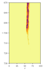
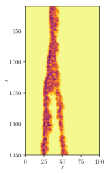
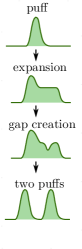
Figure 1: Illustration of puff decay and splitting mechanisms. Left: Decay mechanism—Starting from a puff the system passes close to the decay edge before turning laminar. Splitting mechanism—In the first stage the puff expands into a slug with a turbulent core, in the second stage a laminar gap is formed within the core. The trajectory passes close to the split edge. Trajectories are taken from the stochastic Barkley model.

A comparable dynamical understanding of puff splitting is currently lacking. The directed percolation picture is predicated on splits becoming more frequent than decays with increasing $Re$; However, in the absence of a mechanism for puff splits, it remains unclear if that is the general rule and under what circumstances this type of transition could be absent. In this work we propose the first-ever general mechanism for puff splitting and discuss how it can be suppressed. The mechanism, sketched in Fig. 1 (right), is a two stage process: in the first stage fluctuations drive a puff to expand through a structure called a slug. Slugs are observed at higher $Re$, where puffs are absent, and are similar to puffs except for their expanding core of homogeneous turbulence, see Fig. 2 (right). At the transitional $Re$ we are considering here, we argue that such structures still exist and would contract as illustrated in Fig. 2 (middle). To expand, they must be driven by rare fluctuations. In the second stage, when the slug is wide enough, a laminar pocket forms within the core, separating it into two parts, each of which evolves its own puff. We suggest that this transition is mediated by a state we call the split edge, lying at the boundary between a one-puff and a two-puff state. In the following we motivate the viability of this picture for pipes and other wall bounded flows sharing the same phenomenology. Some of the ingredients in our mechanism have not been directly observed in these flows; we explain why we believe they should be present. We validate the proposed mechanism within the stochastic Barkley model Barkley et al. (2015); Barkley (2016), presenting results taken from simulations, and leave a dedicated study of shear flows by direct numerical simulations to future work. Finally, we identify how the proposed split mechanism could be suppressed, discussing possible signatures.

II The slug-gap-split mechanism

II.1 Expansion stage

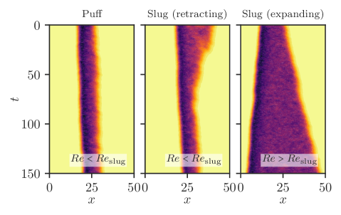
Figure 2: At $Re<Re_{\text{slug}}$, puffs are stable (left). For $Re>Re_{\text{slug}}$, turbulence expands via slugs (right). Slugs also exist for $Re<Re_{\text{slug}}$, but they retract into a puff instead of expanding (center). Realizations taken from the stochastic Barkley model.

We begin by motivating a regime of $Re$ where slugs and puffs coexist for pipe (and duct) flow. A slug is a structure interpolating in space between a homogeneous turbulent state at its core, where turbulence production balances turbulence dissipation, and laminar base flow at its sides. Slugs are observed at $Re>Re_{\text{slug}}$, where they replace puffs. It is also observed that the expansion rate of a slug grows continuously with $Re$, starting from zero at $Re=Re_{\text{slug}}$ Duguet et al. (2010); Barkley et al. (2015). We argue that this continuous transition implies that homogeneous turbulence can first be sustained at $Re<Re_{\text{slug}}$ (referred to as a masked transition in Barkley et al. (2015)), here denoted by $Re_{\text{turb}}$, see Fig. 3. Indeed, that the relative front speed for slugs continuously increases from zero at $Re_{\text{slug}}$ implies that the transition from slugs to puffs with decreasing $Re$ has to do with a change in front speed, rather than with the disappearance of homogeneous turbulence below $Re_{\text{slug}}$. If $Re_{\text{slug}}$ was indeed the point where homogeneous turbulence is first sustained, one would not generically expect front speeds to match there.

Thus, slugs should be well defined dynamical states also in the range $Re_{\text{turb}}<Re<Re_{\text{slug}}$, developing when homogeneous turbulence and laminar flow are brought into spatial contact. The transition from slugs to puffs with decreasing $Re$ is then a consequence of the expansion rate of a slug becoming negative in this range, as is consistent with a continuous decrease in relative front speed starting from zero at $Re_{\text{slug}}$. We thus expect that, once excited, a slug would contract and turn into a puff, as is illustrated in Fig. 2 (middle). Such a contraction of slugs means that laminar flow overtakes homogeneous turbulence for this range of $Re$, implying that the turbulent state is metastable Pomeau (1986).

Note that we expect contracting slugs to be hard to observe in direct numerical simulations or experiments: chaotic fluctuations would quickly split a slug, through the mechanism explained below, if it is too wide. Indeed, contracting slugs have not been observed in shear flows to date. They are also hard to observe in the Barkley model for the classical parameters used in Barkley (2016), where the noise level is much higher than the one we use in Fig. 2. However, if narrow enough, a contracting slug should be an observable dynamical state below $Re_{\text{slug}}$.

For the split mechanism, we propose that the most likely way to expand a puff is for random fluctuations to overcome the retraction of the slug. The first stage of our mechanism is thus the expansion of a puff, via rare chaotic fluctuations, into a slug with a wide enough turbulent core. This first stage is accessible at $Re_{\text{turb}}<Re<Re_{\text{slug}}$.

II.2 Gap formation stage

The second stage corresponds to the transition from a slug with a turbulent core to a state with two puffs. For this stage, only the center of the slug, namely its turbulent core, is relevant. Within this core, to end up with two separated puffs, a laminar gap must be formed by chaotic fluctuations.

When viewed locally, the creation of a laminar gap within turbulent flow is a transition in its own right. Namely from spatially homogeneous turbulence everywhere in the pipe into a state with some laminar flow present. Indeed, homogeneous turbulence should be metastable for $Re<Re_{\text{slug}}$: a laminar-turbulent front would overtake the homogeneous turbulent flow, so that an opened laminar gap would expand and the state would not return to homogeneous turbulence. Along this transition, there should exist a minimal local perturbation of the homogeneous turbulence which will open a gap, and a corresponding mediating edge state: The gap edge, see Fig. 3.

We expect the gap edge to take the form of a local decrease of turbulence down to a threshold value. A further decrease of turbulence would widen the gap until laminar flow is formed, while an increase of turbulence would close it back. In that sense, the gap edge is the minimal nucleus of laminarity to create a lasting gap, mirroring the decay edge between laminar flow and a puff, which is the minimal nucleus of turbulence to create a turbulent puff.

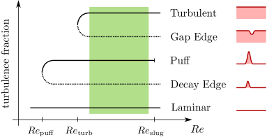
Figure 3: Bifurcation diagram (sketch) for transitional pipe flow. Green shaded region: applicability region of the proposed split mechanism. Attracting states are solid lines, unstable edge states are dotted. Right column: Sketches of the corresponding states. In the deterministic Barkley model used here $r_{\text{turb}}=0.667$ and $r_{\text{slug}}=0.726$.

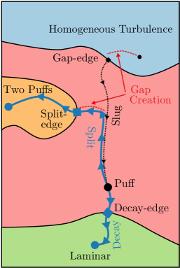
Figure 4: Sketch of the phase space, transitions and edge-states. From the puff basin (red region), the system can decay through the decay edge state into the laminar basin (green region). Alternatively, a puff can split, transitioning through the split edge state into the two puff basin (orange region). The split transition (blue line) consists of: (i) a slug driven by noise to expand, otherwise deterministically contracting (black dotted line), (ii) gap formation within the slug. This gap creation (red dotted) is the same as in the transition out of the homogeneous turbulence basin (blue region).

The terminology gap edge implies that we expect this state to lie on a leaky basin boundary between two long lived states. Indeed, for periodic boundary conditions, that would be the leaky boundary between a puff and a homogeneous turbulent state (which can thus be thought of as the edge of homogeneous chaos). Such a leaky boundary could form as a result of a boundary crisis, where the homogeneous turbulence state touches its basin boundary with the puff, making transitions to the puff state possible. A boundary crisis is also the mechanism believed to give rise to puff decays. Those are mediated by the decay edge, passing through the leaky boundary between the laminar and puff state Skufca et al. (2006); de Lozar et al. (2012). From this point of view, a contracting slug is a dynamically favorable direction from the boundary between homogeneous turbulence and a puff, where the gap edge lies, to the puff see Fig. 4.

To summarize, we argue that after the expansion into a slug, the second stage on the way to a puff split is the above described gap creation, occurring in the turbulent core of the slug.

II.3 The split edge state

Viewed as a whole, the split transition requires crossing the boundary between one and two puffs, motivating yet another edge state—the split edge, see Fig. 4. Combining the two stages of the mechanism, the split edge should roughly take the form of a slug with a gap edge in its core, exactly wide enough to fit it, as sketched in Fig. 1. Indeed, local chaotic fluctuations of the gap edge along its unstable direction can either widen it, inducing a split, or close the gap, forming the core of a slug, which would then retract into a puff.

Here, we are suggesting the existence of a leaky boundary between a single puff and a two-puff state. Transitions from the two puff state to a one puff state are quite natural: they could occur through a decay of one of the puffs, implying an edge state of the form of a puff+decay edge. Such transitions would then be related to a boundary crisis where the two puff state touches the boundary. However, such an edge state does not necessarily allow the opposite transition, from a single puff to two, since the decay edge cannot be spontaneously excited from laminar flow. Instead, we expect such transitions to be mediated by the proposed split-edge state, corresponding to a boundary crisis where the two-puff state touches the boundary. This might explain the exponential distribution of transitions times from the one-puff to the two-puff state observed for puff splitting Avila et al. (2011). The leaky boundary between a one puff and a two puff state can thus include two embedded edge states, one for each direction. This complicates splitting events, since after reaching the two-puff basin, the system can recross the boundary back to a single puff state, giving rise to near-split events.

II.4 Role of fluctuations

In the proposed mechanism, fluctuations have a double role: first, they drive the puff to become a slug and subsequently expand it. Second, when the core of the slug is wide enough to facilitate a gap edge, fluctuations drive the turbulence in the slug core below a threshold. It then generates an expanding laminar hole, with the two remaining segments of turbulence naturally evolving into puffs. Clearly, the expansion stage becomes more likely as $Re$ increases, slugs contracting increasingly slower as $Re_{\text{slug}}$ is approached. On the other hand, gap creation becomes less likely with increasing $Re$, since the homogeneous turbulent state becomes more stable. The latter trend is opposite to observations in straight pipes Avila et al. (2011), implying that if our mechanism is at play, the gap creation is not the limiting factor in its splits. Finally note that the sustainment of the two puff state at the end of the transition may also depend on fluctuations: the decay probability of the downstream puff is increased by close proximity to an upstream puff Hof et al. (2010); Barkley (2016), causing near-split events Gomé et al. (2021); SI .

III Results for the Barkley model

In the remainder, we will demonstrate the relevance of the slug-gap-split mechanism focusing on transitional turbulence in the Barkley model. Each step of the analysis we perform could also be applied to direct numerical simulations of the Navier-Stokes equation, with appropriate adjustments. However, as it is significantly more computationally expensive to generate samples for the latter, here we limit the investigation to the Barkley model. This model is known to successfully reproduce both qualitative and quantitative features of pipe and duct flow Barkley et al. (2015), relying on minimal modeling ingredients. Moreover, in the presence of stochastic noise, the model also goes through a directed percolation transition, facilitated by puff decays and splits Barkley (2016). Note that the deterministic Barkley model does not exhibit chaos nor proper turbulence, but rather captures the underlying phase space structure. In particular, puffs and homogeneous turbulence are deterministic states in the model. Transitions between basins of attraction are then made possible by the inclusion of the noise, which models chaotic fluctuations and allows for leaky boundaries.

The model is one dimensional, describing the coarse grained dynamics along the pipe direction $x$, and employs two variables: the mean shear $u(x,t)$ and turbulent velocity fluctuations $q(x,t)$ Song et al. (2017). Alternatively, $u(x,t)$ can be interpreted as the local centerline velocity, which becomes smaller in the presence of turbulence—namely dropping down to the mean flow rate $\bar{U}$, and is largest for laminar flow at $U_{0}$.

The Barkley model is given by

$$\begin{cases}\partial_{t}q+(u-\zeta)\partial_{x}q=f_{r}(q,u)+D\partial_{x}^{2}q+\sigma q\eta\\ \partial_{t}u+u\partial_{x}u=\epsilon\left[(U_{0}-u)+\kappa(\bar{U}-u)q\right]\\ \end{cases}$$ (1)

where $f_{r}(q,u)=q(r+u-U_{0}-(r+\delta)(q-1)^{2})$. The parameter $r$ is the most important, and plays the role of $Re$. The parameter $D$ controls the strength of turbulence diffusion, $\epsilon$ the (slow) relaxation of the mean flow to the base laminar profile, $\kappa$ the influence of turbulence on the mean flow profile (blunting it), and $\delta$ provides a finite threshold keeping the laminar base flow stable in the limit $r\to infinity$. Lastly, $\eta$ is a spatiotemporal white noise with amplitude $\sigma$. It is multiplicative to mimic the proportionality of chaotic fluctuations in actual flow to the turbulence level present at that point (importantly, turbulence cannot be excited from laminar flow where $q=0$). The values of parameters we choose for our numerical experiments is discussed in section V. The Barkley model has been demonstrated to quantitatively capture features of transitional pipe flow remarkably well Barkley et al. (2015); Barkley (2016).

In the model, the base laminar flow and homogeneous turbulent state (as is present in the core of the slug) are fixed points: $q=0,u=U_{0}$ and $(q_{t},u_{t})$ correspondingly. Our focus is the range $r_{\text{turb}}<r<r_{\text{slug}}$ where the turbulent fixed point coexists with puffs. As sketched in Fig. 3, in the model the turbulent fixed point appears in a saddle node bifurcation at $r=r_{\text{turb}}$ together with an unstable traveling wave—the gap edge state described above. See Anna and Tobias (2022) for a full classification of states.

Before turning to stochastic transitions, we analyze the split edge state lying at the boundary between a one-puff and a two-puff state. We locate the split edge state using edge tracking within the deterministic model. Spatial profiles of $q,u$ for the split edge are shown in Fig. 5 (left). To confirm the proposed mechanism is at play, we have also obtained the gap edge for the model via edge tracking. Superposing the gap edge and a slug with a (momentarily) equal spatial extent onto the split edge indeed gives an almost exact match. This match between the three objects is also shown in a plot in the $q$-$u$-plane in Fig. 5 (right).

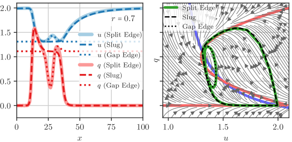
Figure 5: Deterministic edge state between one and two puffs, the split edge (solid), overlaid are a slug (dashed), and a gap edge (dotted). Configurations are shown in space (left) and in the $u$-$q$-plane (right).

IV Stochastic transitions in the Barkley model

Decay and split transitions are made possible via random fluctuations—chaotic in pipe flow and stochastic in the Barkley model—whose rare realizations bring them about. These transitions are thus probabilistic in nature, and so must be the comparison to an underlying dynamical mechanism. We first demonstrate our method of analysis and the required probabilistic notions for decay transitions, which are simpler in nature and are already well understood. We then apply these ideas to test the slug-gap-split mechanism.

IV.1 Puff Decay

We set out to confirm that the decay transition is a trajectory connecting the puff state to the laminar state, crossing the boundary through the decay edge. To that aim, we collect many decay trajectories in the stochastic Barkley model. The average decay path is shown in Fig. 6 as a space-time plot of the average value of $q$ along the transition. It is presented in the frame of reference moving at the average speed of a puff. A visual signature that the trajectory goes through the decay edge is the increase in speed during the decay, the decay edge moving at a speed $\approx U_{0}-\zeta$ Mellibovsky et al. (2009); Duguet et al. (2010); Barkley (2016).

In order to speak about an edge between different states in noisy, stochastic data sets, we further introduce the notion of the stochastic decay edge: This is the set of configurations with the property of having an equal probability to transition to laminar flow or to become a puff. Since all observed decay events happen in a very similar manner, the average of these stochastic decay edge states is a meaningful state itself. Specifically, we obtain the stochastic edge in the following way: given an observed decay trajectory we initiate many stochastic simulations from configurations along it, and measure the likelihood of continuing on the transition. This defines the committor for the given trajectory (see section V). We then identify the configuration from which there is an equal probability to transition or return back, i.e. where the value of the committor is $1/2$. Repeating this for many decay trajectories yields the set of configurations defining the stochastic edge.

We expect the average stochastic edge state to be similar in structure to the deterministic decay edge. This is confirmed in our numerical experiments. Fig. 6(b) (left) shows the spatial profiles of the average stochastic decay edge, averaged over the different trajectories, on top of individual realizations. For comparison, a deterministic decay edge is shown in Fig. 6(b) (right). In 6(a) we show the average transition path alongside the committor, averaged over decay trajectories. Examples of the committor for individual trajectories are presented in the SI (supplementary information).

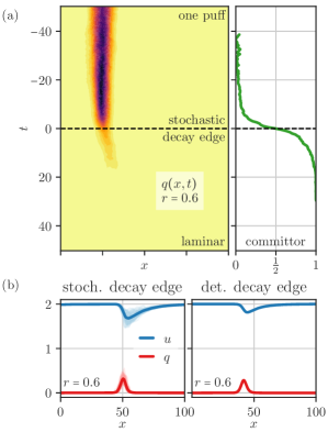
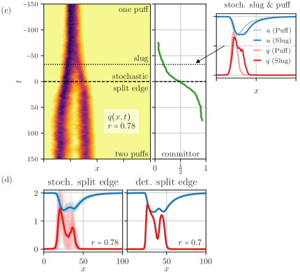
Figure 6: Transitions in the puff regime, $r_{\text{turb}}<r<r_{\text{slug}}$ in the Barkley model where $r$ is a proxy for $Re$. (a) Left: $q(x,t)$ of the average stochastic decay trajectory in space-time. Right: Average committor along the transition. (b) Left: Average stochastic decay edge, corresponding to the dashed line in (a), on top of individual realizations in transparent color. Right: Deterministic decay edge. (c) Left: Average stochastic split trajectory. Right: Average committor. Inset: Average spatial profile at an initial stage of the transition, having a slug-like structure, along with an average puff. (d) Left: Average stochastic split edge, on top of individual realizations. Right: Deterministic split edge.

IV.2 Puff splitting

We can now apply these same ideas to the puff splitting transition. Concretely, to test the relevance of the slug-gap-split mechanism to stochastic transitions in the Barkley model, we will use the average transition path obtained from random puff splits. In Fig. 6(c) we present this average path, where trajectories are aligned according to the location of the stochastic split edge. The latter is obtained using the same algorithm as for the stochastic decay edge; The corresponding average committor is shown in Fig. 6 (c). Note the striking resemblance of the average transition to a single realization of a band split in channel flow in a narrow domain Gomé et al. (2020, 2021). The average transition presented in Fig. 6 (c) indeed reflects the typical splitting trajectory in the Barkley model, such as that in Fig. 1(right); Outliers were included in the averaging but had a negligible effect. Examples of outlier splitting trajectories are shown in the SI.

The average transition path clearly shows the expansion stage of the slug-gap-split mechanism: as seen in the inset of Fig. 6 (c), prior to the creation of the laminar hole the puff extends into a wider turbulent structure. Moreover, this average structure resembles a slug, containing a small homogeneous region most clearly seen in the $u$ profile. Furthermore, the structure always has the same spatial extent right before gap formation, indicating an expansion stage up to the necessary length. To test the gap formation stage, we now compare the average stochastic split edge state to the deterministic split edge. The stochastic split edge is presented in Fig. 6(d) (left) on top of individual realizations, while the deterministic edge is shown Fig. 6(d) (right). There is very good qualitative agreement between the two. Note that the stochastic noise induces parameter shifts, e.g. of $r_{\text{slug}}$, compared with the deterministic model Barkley (2016); SI ; thus we keep the comparison qualitative.

For the parameters used here, we observe that the main bottleneck for the transition is the first stage, expansion of the slug. Indeed, once the slug is wide enough, a laminar gap is likely to form, which smears the gap within the stochastic split edge in Fig. 6 (d) (left). The likelihood of splits is thus dominated by the expansion stage, whose likelihood increases with $r$, as is consistent with observations for the model.

V Methodology for the Barkley model analysis

In the following, we will describe the numerical algorithms we implemented in order to obtain critical points of the dynamics (i.e. stable fixed points and edge states), as well the methodology used to obtain information about the stochastic transition, the ensemble of transition trajectories, the committor function, and the stochastic edge state.

V.1 Stable states

In order to find the stable states (turbulent, puff, laminar) of the Barkley model, we numerically integrate it with parameters $\zeta=0.8$, $\delta=0.1$, $\epsilon=0.1$, $\kappa=2$, $U_{0}=2$, $\bar{U}=1$, and $D=0.5$, additionally with small diffusion coefficient for the velocity $D_{u}=10^{-2}$ which is not expected to affect the results Barkley (2016). The noise amplitude $\sigma$ is $\sigma=0$ for deterministic simulations and $\sigma=0.5$ for stochastic simulations, except in Fig. 2 where $\sigma=0.2$ for demonstration purposes. All numerical simulations are performed in a periodic spatial domain $x\in[0,L]$, with $L=100$.

The functions $q(x)$ and $u(x)$ are discretized on an equidistant computational grid with $N_{x}=128$ or $N_{x}=256$ grid points. Spatial derivatives are computed pseudo-spectrally, by using the fast Fourier-transform. We use exponential time differencing (ETD) Cox and Matthews (2002) as temporal integrator, which is exact for all linear terms, and first order for the nonlinear (reaction) terms. The time-step is chosen between $\Delta t=10^{-2}$ and $\Delta t=10^{-3}$. In order to include stochasticity, we generalize first-order ETD to include the stochastic increment, similar to Kloeden et al. (2011); Lord and Tambue (2013).

The puff, gap edge and split edge are traveling at fixed speed along the pipe, and are therefore not proper fixed points but instead limit cycles of the dynamics. We fix for that by transforming into a moving reference frame adaptively, so that the center of turbulent mass of the objects remains stationary.

V.2 Edge tracking algorithm

To find the unstable fixed points, i.e. the edge states between puff and laminar flow (the decay edge), between puff and two puffs (the split edge), and between turbulent flow and puff (the gap edge), we employ edge tracking. This algorithm integrates forward in time two copies of the system, one in each basin of attraction between which the edge state is to be found. The two copies are kept close via a bisection procedure to converge back to the separating manifold should the states drift too far apart. Effectively, this procedure integrates the system’s dynamics, but restricted to the separating manifold between two stable states. The individual fixed points (laminar, puff, turbulent, two puffs) are identified via their turbulent mass $\bar{q}=\int_{0}^{L}q(x)\,dx$.

V.3 Stochastic transitions

V.3.1 Ensemble of Transition Trajectories

Including stochasticity into the Barkley model, $\sigma\neq 0$, allows the model to transition between different meta-stable states. For example, the puff state is always coexistent with the laminar state, and fluctuations can drive the puff into eventual decay. Numerically, we generate an ensemble of transitions between two states by initializing in one state, and then simulating the stochastic dynamics until another state is observed.

For decays, we identify whether a configuration has entered the laminar state or the turbulent state by checking whether its turbulent mass $\bar{q}$ is within an interval of the expected turbulent mass of the laminar state $\bar{q}=0$ or the turbulent state $\bar{q}=q_{t}$. For the one puff state, we similarly compare the configuration’s turbulent mass to that of the average puff. It is less straightforward to identify the two puff state. Here, we flag a potential puff split event if the fifth Fourier-mode of $q$ exceeds a threshold, which for our parameters was empirically identified to be sensitive to the formation of a gap. Whether a split has indeed taken place is then later checked when computing the committor along the transition and seeing whether it ever reaches one; see section V.3.2. This way, we avoid flagging “near-split” events, where a turbulent region separates from the main puff, but is too small to eventually survive.

V.3.2 Stochastic Edge Tracking

In order to compare edge states between the deterministic model (where edge states can be exactly found, but transitions never happen), and the stochastic model (where noise-induced transitions can be observed, but fixed points can only be identified on average), we develop the notion of the stochastic edge. The underlying intuition comes from the forward committor function known in transition path theory Vanden-Eijnden (2006); E and Vanden-Eijnden (2010): Given a stochastic process $X_{t}$ on some state space $\Omega$, consider two subsets $A\subset\Omega$ the reactant state, and $B\subset\Omega$ the product state. We are interested in transitions of the process from $A$ to $B$. The (forward) committor $p^{+}:\Omega\mapsto[0,1]$ for the transition $A\to B$ denotes the probability that the process visits $B$ next, before visiting $A$. Intuitively, the committor measures how much the system is “committed” to performing the transition. While the committor can be precisely defined for both stochastic and deterministic processes E and Vanden-Eijnden (2010), its computation through solving a Fokker-Planck type equation is prohobitive for any large system. Instead, for stochastic systems such as the Barkley model, the committor can be estimated by sampling many realizations of the process and counting the occurrences of the transition event.

After generating an ensemble of transitions between two attractors as described above in section V.3.1, we can set out to numerically compute the committor along these transition trajectories. One can numerically find the committor of a configuration $(q,u)$ via sampling: Initialize the simulation at $(q,u)$ and sample many times, measuring whether we visit the product state before the reactant state. We do so for many states along each individual transition trajectory. For example, for a stochastic transition between the puff and laminar flow, close to the puff the committor will be almost zero. Close to the laminar state, the committor will be almost one. In between, there is a region where the committor takes intermediate values. We define the stochastic edge of a transition to be a state at which the committor takes the value $\frac{1}{2}$. Note that for a stochastic transition a committor value of $\frac{1}{2}$ can be attained multiple times per transition. In our case, we pick as the relevant stochastic edge the state where the committor is closest to $\frac{1}{2}$ throughout the transition, and take the first such state if there are several.

In practice, for the puff decay transition, we define both the set $A$, the puff, and the set $B$, the laminar state, by thresholding its turbulent mass $\bar{q}$. For the puff split transition, we define the set $A$, the one puff state, and the set $B$, the two puff state, by thresholding the second cumulant under $q$, i.e. $\langle x^{2}\rangle_{q}-\langle x\rangle_{q}^{2}$. This quantity measures to what degree turbulent mass is distributed away from the center of turbulent mass, $\langle x\rangle_{q}$. It is therefore small for the localized one puff state, but large for the two puff state, where the center of mass is located somewhere between the two puffs. The quantity is also large for extended slugs without a gap which might occur during a transition event. To avoid mis-identifying a slug for two puffs, we check the threshold criterion for a prolonged time interval. If the configuration remains above the threshold very long, then it is almost guaranteed to be in the (long lived, stationary) two puff state, instead of the (short lived, transient) extended slug state or other mixed states, which quickly decay.

V.3.3 Averaged Stochastic Transition Path

In order to obtain an average stochastic transition path, we average all individual trajectories of our ensemble of transition trajectories obtained as described in V.3.1. We average the committor of individual trajectories over the ensemble of transition trajectories, by aligning in time the numerically measured committor at the stochastic edge. Note, though, that the average committor is not identical to the committor of the average transition trajectory. We nevertheless show the average committor to give an impression of how fast the transition happens: The sharpness of the transition from 0 to 1 indicates the timescale of the transition itself.

VI Conclusion and Discussion

The subcritical transition to turbulence is generically characterized by the appearance of localized turbulent patches, called puffs in pipe flow, whose proliferation brings about a sustained turbulent phase. Here we have presented the first detailed proposal for the dynamics underlying the proliferation process: a dynamical puff-splitting mechanism termed the slug-gap-split mechanism. We have motivated the relevance of this mechanism for pipe flow, and confirmed its presence in the Barkley model. The proposed slug-gap-split mechanism implies concrete predictions, making the proposal testable. Moreover, it introduces a novel framework within which previous observations could be interpreted, and alternatives for other wall-bounded flows could be explored. We now discuss these issues in detail.

Previously, splitting had been observed to occur through the following process Avila et al. (2011); Shimizu et al. (2014); Mukund and Hof (2018): The puff continuously emits vortices (turbulence) from its leading edge, then, if this patch of vortices manages to persists and sufficiently separate from the parent puff, it seeds a new puff. These observations could be consistent with the slug-gap-split mechanism, with the growth of the daughter puff occurring after the crossing of the phase space boundary between a single puff and two. The possible subsequent decay would then correspond to a near-split event, a recrossing of this boundary. Still, such observations could also imply that a different mechanism is at play, whereby a puff emits a turbulent patch without going through an expansion stage first. An expansion stage where a small core of balanced turbulence forms within the puff is thus a distinct prediction of the slug-gap-split mechanism. Only then does a laminar gap appear in this picture, and the structure evolves towards two puffs. The latter process can then sometimes fail if the downstream puff is snuffed out by the upstream one. It is worth noting that the splitting process looks much less symmetric in pipe flow compared to that in the Barkley model. That, however, might be a visual artifact: the Barkley model does not capture the very steep increase in turbulence level observed at an upstream front, making the puff appear more symmetric and thus also the splitting process. This quantitative feature should not influence the applicability of the slug-gap-split mechanism, which does not rely on it. In fact, the results presented in Ref. Shimizu et al. (2014) for the centerline velocity during a split in pipe flow do seem to indicate a split through the formation of a laminar gap within turbulent flow, though further study is needed.

To distinguish between the different mechanisms that could be at play for splits, the analysis outlined above for the Barkley model could be carried out in direct numerical simulations. First, the split edge state could be located using edge tracking, as previously done for the decay edge state Schneider et al. (2007); Mellibovsky et al. (2009); Duguet et al. (2010). Second, a probabilistic analysis of split transitions using the committor between one and two puffs, akin to the one introduced here, could also be carried out. It would reveal the average transition path and the stochastic edge state, which could be compared with the expectations from the slug-gap-split mechanism. Note that the stochastic edge state, defined here directly via transitional trajectories, is not a-priori identical to the split edge state found via edge tracking. The comparison between the two would test the role played by the latter in the transitions.

The slug-gap-split mechanism is restricted to the range $Re_{\text{turb}}<Re<Re_{\text{slug}}$. This suggests a novel possibility that more than a single splitting mechanism exists, and that different mechanisms could dominate at different $Re$. It would thus be interesting to assess $Re_{\text{turb}}$ for pipe flow, e.g. using a minimal flow unit Jiménez and Moin (1991); Hamilton et al. (1995), and comparing it to the Reynolds number at the directed percolation critical point. Indeed, while we expect our mechanism to dominate close to $Re_{\text{slug}}$, it is not guaranteed to survive down to the critical point. At lower $Re$ it could in principle be replaced by a process whereby a puff emits a turbulent patch, as described above. The split edge state would then take a different character SI .

While we have focused on pipe flow so far, other wall bounded flows which exhibit a subcritical transition to turbulence (and have a single extended direction) are captured within the same framework. Indeed, splits in Couette and channel flow in a narrow domain seem to follow the proposed mechanism: an expansion stage is observed, followed by the formation of a laminar gap Shi et al. (2013); Gomé et al. (2020, 2021). Generally, the key condition for the slug-gap-split to be relevant is for the expansion rate of turbulence to continuously increase with Re, starting from zero at the transition from puffs to slugs.

Our work offers a novel point of view on how the phenomenology of other wall bounded flows could differ from that of pipe flow. In particular, we now discuss a mechanism by which splits could be suppressed compared to decays, and therefore a directed-percolation-type transition would be impossible. This could be relevant for slightly bent pipes Rinaldi et al. (2019); Barkley (2019). In the slug-gap-split mechanism the likelihood of the transition is the multiplication of that of the expansion stage, which increases with $Re$, and of the gap creation stage, which decreases with $Re$. If the latter is sufficiently high close to $Re_{\text{slug}}$ then transitions would become more likely with $Re$, as observed in pipes. However, splitting could be limited by gap creation if such creation becomes improbable at a sufficiently low $Re$. Then, splits would become less likely with increasing $Re$ and would be most difficult to observe close to $Re_{\text{slug}}$. The occurrence of a directed percolation critical point requires that the probability of puff splitting roughly balances that of puff decay. Such a balance is not guaranteed if, for large enough Reynolds numbers, both decays and splits become increasingly improbable with $Re$. Splits could then remain less probable than decays for the entire range of $Re$.

A signature that gap creation is indeed a limiting factor for puff splits would be the absence of an intermittent turbulent regime above $Re_{\text{slug}}$. This regime, observed in pipe flow Moxey and Barkley (2010), is characterized by laminar gaps randomly opening within the homogeneous turbulent state, persisting and randomly closing. Indeed, if reaching the gap edge is prohibitively improbable for splits, such laminar gap excitations would also be suppressed Anna and Tobias (2022). In fact, such a correlation seems to exist for slightly bent pipes Rinaldi et al. (2019), providing a tantalizing connection to the suggested scenario.

Acknowledgments We thank Dwight Barkley, Sébastien Gomé and Laurette Tuckerman for helpful discussions and comments. We are additionally grateful for input from Yariv Kafri, Dov Levine and Grisha Falkovich.TG acknowledges support from EPSRC projects EP/T011866/1 and EP/V013319/1.

Appendix A Noise in the Barkley model

As mentioned in the main text, introducing noise changes the attracting states and their range of existence as compared with the deterministic dynamics. In particular, front speeds are changed leading to a change in $r_{\text{slug}}$ so that puffs exist in the stochastic model in a range of $r$ above that of the deterministic model, see also Barkley (2016). Evidently, a direct comparison between deterministic and stochastic states at the same $r$ e.g. for the the split edge, without properly taking into account the effect of noise on the deterministic structures, is precluded.

However, the mechanisms presented in the main text do not depend on such noise effects, even if the realizations of the fluctuations needed to drive them might. Clarifying the effect of noise on the invariant solutions of the deterministic model and their regime of validity, as well as how such changes may affect transition probabilities and realizations, is left for future work.

Appendix B Example transitions with committor values

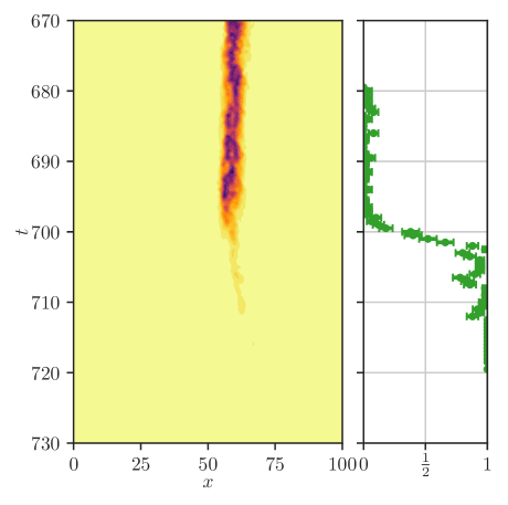
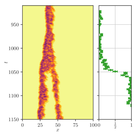
Figure 7: Left: Single stochastic puff decay trajectory, together with its committor along the transition. The stochastic edge, at committor value $\frac{1}{2}$, marks the halfway point along the transition, where there is an equal probability of continuing to decay, or returning back to the puff.
Right: Single stochastic puff split trajectory, together with its committor along the transition. The stochastic edge, at committor value $\frac{1}{2}$, is exactly the point at which the puff has elongated into a slug, and a gap starts to appear. It demarks the point at which returning to a single puff is as likely as continuing to split into two.

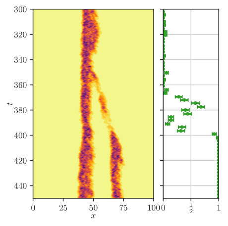
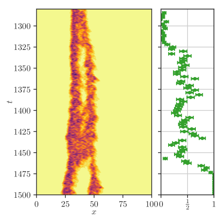
Figure 8: Left:Unusual stochastic puff split trajectory, together with its committor along the transition. During the initial split, only a very faint puff separates, and is almost snuffed out again at $t\approx 390$. If it had disappeared, it would have been a “near-split” event, exhibiting a separating puff that is not able to survive. Instead, in this case, a rare fluctuation revives the separating puff to full strength, and the committor grows again.
Right: Unusual stochastic puff split trajectory, together with its committor along the transition. While the initial split looks typical, the trajectory re-merges into a very wide slug, skirting the committor-$1/2$ region for a very long time until eventually separating. Indeed, at $t\approx 1460$, the secondary puff did almost decay.

Figure 7 (left) depicts a single puff decay trajectory alongside its numerically determined committor function. For $N_{\text{conf.}}=75$ configurations along the transition, we took $N_{\text{samples}}=50$ samples to determine the probability that the process, initialized at that state, would eventually end up in the puff state or the laminar state. Similarly, figure 7 (right) shows the same for a single puff split trajectory. Here it is visible how the committor takes value $\frac{1}{2}$ exactly at the point where the gap starts to get created. Before this point, the process is more likely to return to a single puff (by retracting the elongated slug state it is in), while after this point, the process is more likely to continue on with its split into two puffs by widening the gap between them.

While most split trajectories qualitatively resemble figure 7 (right), the interaction of dynamics and noise allow for much more complicated split trajectories. One class of phenomena are near-split events, where a secondary puff splits off but is ultimately too small to survive. Since we condition our split transitions on finally arriving at two puffs, these near-splits are not included in the ensemble of split transition trajectories. Yet, its remnants can be felt, as visible for example in figure 8 (left), where a near-split almost occurs, but is eventually averted. The single puff splits into two, but the secondary puff is barely able to survive. As indicated by the committor function, it would have been far more likely for the secondary puff to decay again. The chance fluctuation averted the decay, though, and we do end up with two puffs. In some examples, such as in figure 8 (right), split transitions meander for an extended time near the committor-$1/2$-boundary, here, for example, by first splitting, but re-merging into an unusually wide slug, that eventually splits again. We stress that for our transition trajectory ensembles we do not filter out these more complicated events, but instead stick to the procedure outlined above, and include them in our averages. While this increases fluctuations around the observed average transition trajectory and stochastic split edge, it highlights the fact that these unusual events are comparably unimportant, and are dominated by the main mechanism that we describe.

Appendix C Edge state for the transition from two puffs to one

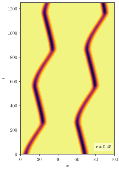
Figure 9: Edge state between the basins of attraction of the one-puff state and the two-puff state. Generally, these edge states consist of the coexistence of a puff and a decay edge. Since both travel at different speed, the resulting (hyperbolic) limiting structure cannot be simply a limit cycle in translation. Instead, puff and decay edge interact and interchange roles after interaction. This is shown for $r=0.45$ (left), where the interaction range is quite long, and $r=0.65$ (right), where the interaction range is shorter and proper collisions are observed.

Figure 10: Close-up of the collision portion of the limit cycle on the edge between the one- and two-puff states for $r=0.68$.

The main material discusses the edge state for a “puff split”: the transition between a single puff and a pair of puffs. For the reverse transition, i.e. from two puffs to one, a more obvious route would be the decay of one of the puffs through the single puff decay mechanism, with the other puff remaining unchanged. An associated edge state intuitively would be comprised of a puff and a separate decay edge state far away from it. In fact, though, such an edge state is quite complicated. The reason is the following: as highlighted in the main material, the speed of the decay edge is different from that of the puff. If we have two puffs present, and want to destroy one of them, we cannot easily have a stationary state comprised of a puff and a decay edge, since the two travel at different speeds. In a periodic domain, they would eventually collide. A fixed point on the border between a single puff and two puffs can therefore not simply be a jointly advected combination of puff and decay edge. Instead, the edge state is a more complicated limit cycle, with co-existence of a puff and a decay edge at some times, but also collisions between the two along this limit cycle.

Because of that, the state is no longer a relative fixed point. Indeed, it is no longer enough to correct for the travel speed of the edge structure globally, as it consists of multiple, possibly interacting structures traveling at different speeds. In the projected coordinate system that eliminates global advection, the edge state remains a limit cycle. We can still employ the edge tracking algorithms to restrict the dynamics to the separatrix between the two basins of attraction, which will consequently evolve into the complicated periodic structure described above. The result of this can be seen in figure 9, where the evolution of $q$ is shown along the hyperbolic edge state, which is indeed periodic (up to spatial translation). It can be seen that for prolonged periods of time, this edge state indeed corresponds to a pair of puff and decay edge, but once their distance becomes too small, they start interacting, the result of which is an exchange of their roles: The puff becomes a decay edge, and the decay edge a puff. For $r=0.45$, as in figure 9 (left), this interaction happens over considerable distance, while for $r=0.65$ (see figure 9 (right)), the two collide. Generally, the two are allowed to approach closer the higher the $r$. Figure 10 shows a close-up of a collision between a decay edge and a puff that forms a puff and a decay edge after the interaction.

Increasing $r$ further, the edge state becomes a single advected structure, namely the split edge described in the main material. This configuration is an unstable fixed point and is advected without deformation. Remnants of the above limit cycle on the separating manifold still remain, though: The dynamics on the separatrix during edge tracking quickly converge to a joint puff and decay edge state, which then slowly evolves until collision, forming the split edge. We thus hypothesize that the two-to-one-puff transition would never come close to the split edge state described in the main material, and instead transition through a state of the form of a puff plus decay edge, which is no longer an invariant state of the system but a remnant of the limit cycle at lower $r$. This highlights the fundamental irreversibility of the system, where forward and backward transitions are happening with completely different pathways and mechanisms.

In the Barkley model, the structure of the split edge state thus changes with $r$ from that where a puff emits a decay edge, as seen in Figs.9 to the slug+gap structure described in the main material. The two different edge states thus probably correspond to two different mechanisms: the slug-gap-split mechanism which includes an expansion stage and is applicable only above $r_{\text{turb}}=2/3$, and a mechanism where the puff emits a decay edge. In the latter, the split transition is expected to happen through the point in the limit cycle where the two structures are close by. In the Barkley model, the limit cycle split edge state and the (relative) fixed point split edge state merge a little above $r=0.68$, see Fig. 10 where the collision lasts for a while and visually resembles the slug-plus-gap edge state. Thus, it appears that the split mechanism whereby a puff emits a decay edge could be relevant at lower $r$, below or close to $r_{\text{turb}}$, and is replaced by the slug-gap-split mechanism once it becomes available.

Appendix D Comments on the structure of the split edge state in the Barkley model

In the main text, we have motivated that the split edge should take the form of a slug with a gap edge in its core. We have also demonstrated that such a structure is indeed very close to the profile of a deterministic split edge. However, the actual structure of the split edge is subtler, since it must be an invariant solution of the dynamics, in particular a relative fixed point (though there is a range of $r$ where we observe an edge state in the form of a relative periodic orbit as described above). This composite object can indeed move in unison since the speed of the gap edge equals the speed of the turbulence in the core of a slug. However, if the downstream front was truly that of a slug, then the split edge would expand. Instead, the downstream front, which connects directly to the gap edge, must be closer to that of the puff in structure, the speed of the downstream front of a puff matching the upstream front and allowing the split edge to remain stationary in structure. For the value of $r$ shown (and generally where splits are sufficiently probable to be reasonably observed) $u_{t}$ is close to $u_{p}$ so that it would be hard to distinguish between the two fronts visually, though some deviations from a structure of a slug are indeed observed at the point where the downstream front joins the gap edge, as is expected from the above argument.

References

- Reynolds (1883) O. Reynolds, Proc. R. Soc. 35 (1883), 10.1098/rspl.1883.0018.
- Lindgren (1957) E. R. Lindgren, Arkiv fysik 12 (1957).
- Wygnanski and Champagne (1973) I. J. Wygnanski and F. Champagne, Journal of Fluid Mechanics 59, 281 (1973).
- Darbyshire and Mullin (1995) A. G. Darbyshire and T. Mullin, Journal of Fluid Mechanics 289, 83 (1995).
- Avila et al. (2011) K. Avila, D. Moxey, A. de Lozar, M. Avila, D. Barkley, and B. Hof, Science 333, 192 (2011).
- Barkley et al. (2015) D. Barkley, B. Song, V. Mukund, G. Lemoult, M. Avila, and B. Hof, Nature 526, 550 (2015).
- Barkley (2016) D. Barkley, Journal of Fluid Mechanics 803 (2016), 10.1017/jfm.2016.465.
- Pomeau (1986) Y. Pomeau, Physica D: Nonlinear Phenomena 23, 3 (1986).
- Mukund and Hof (2018) V. Mukund and B. Hof, Journal of Fluid Mechanics 839, 76 (2018).
- Manneville (2016) P. Manneville, Mechanical Engineering Reviews 3, 15 (2016).
- Tuckerman et al. (2020) L. S. Tuckerman, M. Chantry, and D. Barkley, Annual Review of Fluid Mechanics 52, 343 (2020), https://doi.org/10.1146/annurev-fluid-010719-060221 .
- Shi et al. (2013) L. Shi, M. Avila, and B. Hof, Phys. Rev. Lett. 110, 204502 (2013).
- Lemoult et al. (2016) G. Lemoult, L. Shi, K. Avila, S. V. Jalikop, M. Avila, and B. Hof, Nature Physics 12, 254 (2016).
- Chantry et al. (2017) M. Chantry, L. S. Tuckerman, and D. Barkley, Journal of Fluid Mechanics 824, R1 (2017).
- Klotz et al. (2022) L. Klotz, G. Lemoult, K. Avila, and B. Hof, Phys. Rev. Lett. 128, 014502 (2022).
- Skufca et al. (2006) J. D. Skufca, J. A. Yorke, and B. Eckhardt, Phys. Rev. Lett. 96, 174101 (2006).
- de Lozar et al. (2012) A. de Lozar, F. Mellibovsky, M. Avila, and B. Hof, Phys. Rev. Lett. 108, 214502 (2012).
- Budanur et al. (2019) N. B. Budanur, A. S. Dogra, and B. Hof, Phys. Rev. Fluids 4, 102401 (2019).
- Rolland (2018) J. Rolland, Phys. Rev. E 97, 023109 (2018).
- Schneider et al. (2007) T. M. Schneider, B. Eckhardt, and J. A. Yorke, Phys. Rev. Lett. 99, 034502 (2007).
- Duguet et al. (2008) Y. Duguet, A. P. Willis, and R. R. KerswellL, Journal of Fluid Mechanics 613, 255 (2008).
- Mellibovsky et al. (2009) F. Mellibovsky, A. Meseguer, T. M. Schneider, and B. Eckhardt, Phys. Rev. Lett. 103, 054502 (2009).
- Avila et al. (2013) M. Avila, F. Mellibovsky, N. Roland, and B. Hof, Phys. Rev. Lett. 110, 224502 (2013).
- Duguet et al. (2010) Y. Duguet, A. P. Willis, and R. R. Kerswell, Journal of Fluid Mechanics 663, 180 (2010).
- Hof et al. (2010) B. Hof, A. De Lozar, M. Avila, X. Tu, and T. M. Schneider, science 327, 1491 (2010).
- Gomé et al. (2021) S. Gomé, L. S. Tuckerman, and D. Barkley, arXiv preprint arXiv:2109.01476 (2021).
- (27) .
- Song et al. (2017) B. Song, D. Barkley, B. Hof, and M. Avila, Journal of Fluid Mechanics 813, 1045 (2017).
- Anna and Tobias (2022) F. Anna and G. Tobias, (2022), https://doi.org/10.48550/arXiv.2111.00233.
- Gomé et al. (2020) S. Gomé, L. S. Tuckerman, and D. Barkley, Phys. Rev. Fluids 5, 083905 (2020).
- Cox and Matthews (2002) S. Cox and P. Matthews, Journal of Computational Physics 176, 430 (2002).
- Kloeden et al. (2011) P. E. Kloeden, G. J. Lord, A. Neuenkirch, and T. Shardlow, Journal of Computational and Applied Mathematics 235, 1245 (2011).
- Lord and Tambue (2013) G. J. Lord and A. Tambue, IMA Journal of Numerical Analysis 33, 515 (2013).
- Vanden-Eijnden (2006) E. Vanden-Eijnden, in Computer Simulations in Condensed Matter Systems: From Materials to Chemical Biology Volume 1, Lecture Notes in Physics, edited by M. Ferrario, G. Ciccotti, and K. Binder (Springer, Berlin, Heidelberg, 2006) pp. 453–493.
- E and Vanden-Eijnden (2010) W. E and E. Vanden-Eijnden, Annual Review of Physical Chemistry 61, 391 (2010).
- Shimizu et al. (2014) M. Shimizu, P. Manneville, Y. Duguet, and G. Kawahara, Fluid Dynamics Research 46, 061403 (2014).
- Note (1) Indeed, when the turbulence level at the upstream front is accentuated for the Barkley model, as done in Barkley (2016), splits in the Barkley model look very similar to those in pipe flow.
- Jiménez and Moin (1991) J. Jiménez and P. Moin, Journal of Fluid Mechanics 225, 213 (1991).
- Hamilton et al. (1995) J. M. Hamilton, J. Kim, and F. Waleffe, Journal of Fluid Mechanics 287, 317 (1995).
- Rinaldi et al. (2019) E. Rinaldi, J. Canton, and P. Schlatter, Journal of Fluid Mechanics 866, 487 (2019).
- Barkley (2019) D. Barkley, Journal of Fluid Mechanics 872, 1 (2019).
- Moxey and Barkley (2010) D. Moxey and D. Barkley, Proceedings of the National Academy of Sciences 107, 8091 (2010).