Access Trends of In-network Cache for Scientific Data

Abstract.

Scientific collaborations are increasingly relying on large volumes of data for their work and many of them employ tiered systems to replicate the data to their worldwide user communities. Each user in the community often selects a different subset of data for their analysis tasks; however, members of a research group often are working on related research topics that require similar data objects. Thus, there is a significant amount of data sharing possible. In this work, we study the access traces of a federated storage cache known as the Southern California Petabyte Scale Cache. By studying the access patterns and potential for network traffic reduction by this caching system, we aim to explore the predictability of the cache uses and the potential for a more general in-network data caching. Our study shows that this distributed storage cache is able to reduce the network traffic volume by a factor of 2.35 during a part of the study period. We further show that machine learning models could predict cache utilization with an accuracy of 0.88. This demonstrates that such cache usage is predictable, which could be useful for managing complex networking resources such as in-network caching.

1. Introduction

The increasing volume of data from scientific experiments and simulations requires a vast amount of resources to store and distribute to geographically distributed users. Many collaborations such as the Large Hadron Collider (LHC) utilize tiered systems to replicate the data in a few places, and the users could access their nearby storage sites. However, with the increasing cost of managing storage resources and the limited number of replicas, the large number of user accesses still create considerable demand on the wide-area network that increases the cost of data analyses, and could cause large-scale network traffic congestion (Espinal et al., 2020; Brown et al., 2020).

In many cases, we observe that a significant portion of the dataset is transferred multiple times over the network for various reasons. To take advantage of this resue, the High-Energy Physics (HEP) community has established a number of regional storage caches (Fajardo et al., 2018; Espinal et al., 2020; Pordes et al., 2007). Analyses show that these caches could significantly reduce the data access latency as well as the traffic on the internet backbone (Copps et al., 2021).

In the example of the HEP community, the largest data source is the LHC instrument at CERN in Switzerland. The main collaborations involved in generating and analyzing these data, known as ATLAS and CMS. Their Tier-1 storage sites in the US are at Brookhaven National Laboratory and Fermi National Accelerator Laboratory respectively. The wide-area network traffic for retrieving and replicating their data is primarily carried on the Energy Science Network (ESnet), one of the key components of the internet backbone especially designed for our nation’s science and research communities. Because the data lakes have demonstrated their effectiveness in reducing the load on the internet backbone, we are interested in exploring the predictability of their impact and the potential for providing a more general distributed storage caching strategy known as in-network caching (Li et al., 2013; Kalla and Sharma, 2016; Sim et al., 2022).

More specifically, our work starts with a study of data access trends with one of the data lakes named Southern California Petabyte Scale Cache (SoCal Repo) (Fajardo et al., 2018). We examine the trends of network traffic volume and establish a machine learning model to predict the future network bandwidth requirement for the regional data cache.

The key contributions of this paper can be summarized as follows: (1) our study finds find that the SoCal Repo was able to reduce the traffic by 23% over the study period, and by 57% under normal usage; (2) this network traffic reduction is stable and predictable by LSTM, with 88.4% accuracy; (3) because of the network traffic reduction, we recommend a general in-network cache to supplement the existing data lakes from HEP to benefit all science user communities.

2. Background

Southern California Petabyte Scale Cache (SoCal Repo) (Fajardo et al., 2018) is a regional ”Data Lake” (Espinal et al., 2020; Pordes et al., 2007) based on XCache (Weitzel et al., 2019; Bauerdick et al., 2014; Fajardo et al., 2018). XRootD system is the bases for the XCache, and supports unique capabilities for data distribution and access, especially for large collaborations such as the Large Hadron Collider (LHC) (Dorigo et al., 2005; Bauerdick et al., 2012). SoCal Repo consists of 24 data cache nodes at Caltech, UCSD, and ESnet with approximately 2.5PB of storage capacity, supporting client computing jobs for High-Luminosity Large Hadron Collider (HL-LHC) analysis in Southern California. In this cache installation, there are 11 nodes at Caltech with storage sizes ranging from 96TB to 388TB; 12 nodes at UCSD with 24TB each node; one node at an ESnet endpoint at Sunnyvale, CA with 44TB of storage. The two southern California sites are within 200 km from each other and have a round trip time (RTT) of less than 3 milliseconds (ms) from each other, while the ESnet node is about 700 km away from UCSD, with an RTT of about 10ms. One node at Caltech is designated for NANOAOD and all other cache nodes are for MINIAOD (Rizzi, Andrea et al., 2019).

When a user’s computing job needs a file from SoCal Repo, the system first looks up the location of the file using the ”Trivial File Catalogue” (TFC) (Fajardo et al., 2020; Fajardo, Edgar et al., 2020). Following the established convention for the tiered storage system, the data files are grouped into the namespace for the local cache nodes and the TFC points to a ”local redirector” in XRootD where the ”local redirector” knows all regional caches. If one of the cache nodes has the file, the redirector routes the application request to the node. If none of them has the file, one of them is told to invoke an XRootD client to fetch the file. The XRootD client is configured to get the file from the national XRootD data federation to the local cache node. Local cache nodes do not connect to another cache node but always connect to the higher tier of the federation. In CMS collaboration, data federation is hierarchical where the US is one flat layer and the rest of the world is another flat layer. By design, each file available to the CMS collaboration has at least a copy somewhere in the US. Thus it is possible to find a copy of any file needed for analysis even though the lookup mechanism in TFC does not always guarantee to recommend a replica in the US.

Most of the file reads in CMS based on XRootD are vectors of byte ranges, and a cache miss leads to a vector of byte ranges getting fetched. When new cache nodes have been added to the local cache nodes, all cache misses go to the new cache nodes first, so that the distributed cache nodes avoid deletions of old data as long as there is a new space to fill. It means that cache nodes that have been around for some time will tend to have data that is not of interest to as many users, and those data will eventually get deleted when running out of space. Adding more cache nodes to an already full distributed cache invariably leads to skewed distributions of data access patterns. This happened around Aug. 26, 2021 when 7 new nodes at Caltech (xrd 3-8, 11) are added to the system, and around Sep. 30, 2021 when 2 new nodes at Caltech (xrd 9-10) are added to the system. The new cache nodes get the new data. The new data is of more interest and leads to more accesses. Old data does not get deleted as there is still space on the new nodes. At some point, it will resolve itself, but may take some time to resolve.

3. Data Access Trends

Our work is based on monitoring information collected from the SoCal Repo between July 2021 and January 2022. The collected information includes the following attributes about every data access request: user id, file id, file path, file size, the data transmission start time, the data transmission finished time, the total size of the transmission, whether the data request is a data transfer (cache miss) or data share (cache hit), which cache node the request is sent to, whether the transmission is successful, and so on. A total of about 7.5 million data access requests are included in this study.

Table 1. Summary statistics for data accesses

	# of Accesses	Data Transfer Size (TB)	Shared Data Size (TB)	Net  Traffic Reduction
July 2021	1,182,717	385.78	519.25	57.37%
Aug 2021	1,078,340	206.94	313.46	60.23%
Sep 2021	1,089,292	206.96	257.18	55.41%
Oct 2021	1,058,071	412.18	141.91	25.61%
Nov 2021	878,703	649.30	82.67	11.29%
Dec 2021	983,723	1,257.89	130.03	9.37%
Jan 2022	1,207,332	2,238.59	148.26	6.21%
Total	7,478,178	5,357.67	1,592.79	22.91%
Daily Average	35,441.60	25.51	7.55	22.83%

Table 1 shows the basic statistics about the data accesses to all cache nodes during the study period (from July 2021 to Jan. 2022). If an ”access” could be satisfied with a file in a cache, then it is a cache hit. On the other hand, if the requested file needs to be retrieved from a remote storage site, then it is a cache miss. Cache miss would require a data file to be transferred from a remote site over the wide-area network. The ”Data Transfer Size” in the table is the total volume of data transferred to satisfy the cache misses. The ”Shared Data Size” refers to the total volume from the cache hits. The ”Net Traffic Reduction” is the percentage of network traffic reduction by the cache system, calculated monthly by (shared data size) / (total access size).

Table 1 shows the net traffic reduction was about 60% during the first three months of the observation, but dropped to as low as 6% in January 2022. This drop is due to a usage change among the physicists in the region, as some users are streaming data through the caching system.

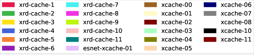
Figure 1. Legend for each node in the regional cache

Figure 1 indicates the color for each node in all the following plots unless specified otherwise.

The monitoring system had troubles on Nov. 24, 2021, and from Dec. 15, 2021 to Dec. 18, 2021. So there are no data during these periods, showing gaps in the following daily plots during these periods.

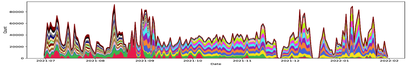
(a) Daily

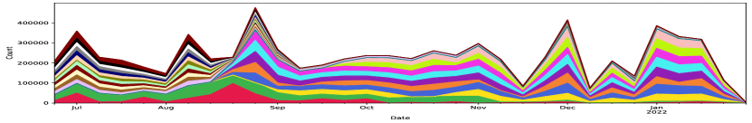
(b) Weekly

Figure 2. Total data access counts in the regional cache. The number of access is relatively stable during the time period of this study.

Figure 2a shows the daily total data access counts, combining the number of date shares (i.e. cache hits) and data transfers (i.e. cache misses), and the distribution among the cache nodes. Figure 2b shows the weekly total data access counts and distribution among the cache nodes.

The number of total accesses is fairly consistent throughout the study period, fluctuating around 31,000 per day. Each cache node evenly receives file requests before September 2021. When new cache nodes have been added to the regional cache, many of the cache accesses have been sent to the new cache nodes evenly with the previously described reason in Section 2.

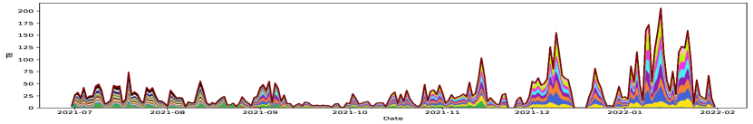
(a) Daily

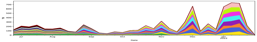
(b) Weekly

Figure 3. Total data access sizes in the regional cache

Figure 3a shows the daily total data access sizes, combining shared data sizes (i.e. cache hits) and transferred data sizes (i.e. cache misses) on each cache node. Figure 3b shows the weekly total data access sizes among cache nodes. The total access size is increasing over the study periods indicating that the requested data size grows while the number of accesses remains about the same each month. When traffic is relatively small, the daily traffic volume is about 21TB per day. After new cache nodes have been added to the regional cache, many of the data access traffic have been sent to the new cache nodes, and it is expected by the policy described in Section 2.

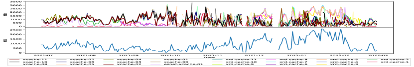
(a) Daily

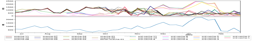
(b) weekly

Figure 4. Average data size per access in the regional cache

Figure 4a shows the average data sizes per access, calculated daily by ${(Total\ Data\ Access\ Size)}/{(Total\ Data\ Access\ Counts)}$. Figure 4b shows the weekly average data sizes per access. The upper parts of both daily and weekly plots show the average data size per access for each node, and the lower parts show the average data size per access of all nodes combined. The average data size per access of all cache nodes gradually decreases since Nov 2021. Overall, the average data size per access is increasing during the study period, consistent with the increases in the total access size while the data access counts remain about the same each month.

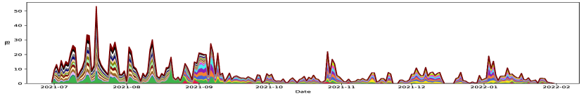
(a) Daily

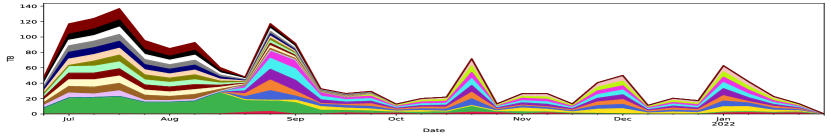
(b) Weekly

Figure 5. Total sizes of the cache hits in the regional cache

Figure 5a and 5b show the daily and weekly total shared data sizes among the cache node respectively. The total shared data size shows a big drop since mid Sept. 2021, with only a few occasional hikes. After new cache nodes have been added to the regional cache, most of the cache hits have been sent to new cache nodes as the new nodes have recent data of more interest.

Figure 6. Daily proportion of cache miss sizes (orange area) and cache hit sizes (blue area) in the regional cache. The cache hit rate reduces after October 2021 because of a usage pattern change.

Figure 6 shows the proportion of the daily total data size of the cache misses. The sudden drop in the daily proportion of cache hit sizes and the gradually increasing cache miss sizes are due to changes in the access trend that several users are constantly streaming data.

j

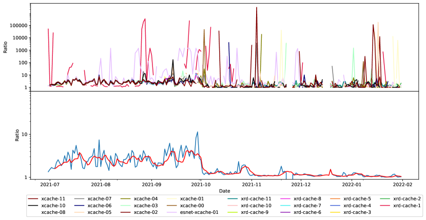
Figure 7. Daily network traffic demand reduction. The average reduction rate is 2.35 before October 2021 and 1.11 afterward.

The network traffic demand reduction rates, calculated by the eqn. (1), are shown in Figure 7 with the red line indicating the 7-day moving average of the network traffic demand reduction rate. The traffic demand reduction rate is the ratio of data volume users access and the volume transferred over the backbone network. It shows that the network traffic demand reduction rate experiences a sudden drop since Oct. 2021 when the user access trends changes to streaming many new data files. The average network traffic demand reduction rate is 1.30 during the study period, while the average rate from July 2021 to Sep. 2021 is 2.35 before the user access trends change. The average rate drops to 1.11 from Oct. 2021 to Jan. 2021, as user streaming data have a great negative impact on the statistics of the caching system.

(1) $$\text{network traffic demand reduction rate}=\\ \frac{\text{(total cache hit size + total cache miss size)}}{\text{(total cache miss size)}}$$

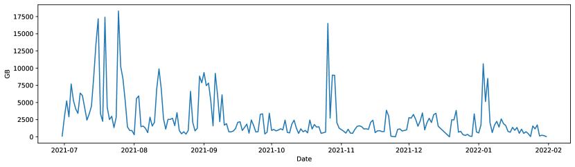
(a) Daily total data reuse size

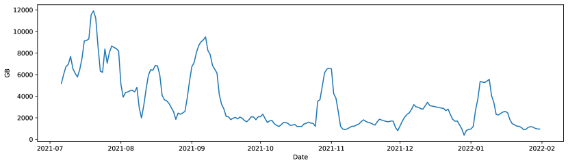
(b) Daily total data reuse size with 7-day moving average

Figure 8. Daily total data reuse size in the regional cache

Figure 8a shows the daily total data reuse size for all nodes in the regional cache. Data reuse means the re-access of the same data file without transferring within the same day (i.e. successive cache hits on the same data without a cache miss on that data during one day. Data reuse indicates the network traffic savings on files that are accessed multiple times. The total data reuse size is the total size of data reused in a single day. Figure 8b shows the daily total data reuse size of 7-day moving average in the regional cache. Prior to Oct. 2021 before the user behavior changes, the total data reuse size generally follows the access size. Since then, the total data reuse size is relatively stable with a few spikes in the middle.

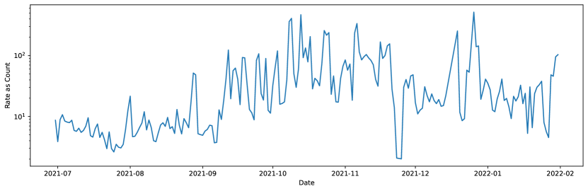
(a) Daily data reuse rate

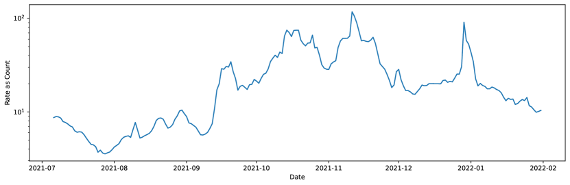
(b) Daily data reuse rate with 7-day moving average

Figure 9. Daily data reuse rat. Despite the significant volume of data being streamed through this cache, there are still significant amount of reuse of files in cache.

Figure 9a shows the daily data reuse rates for all nodes in the regional cache. The data reuse rate is the number of times that the files have been reused in a single day, calculated by
${(Total\ Data\ Reused\ Count)}/{(Number\ of\ Unique\ Reused\ Files)}$.
Figure 9b shows the daily data reuse rate of the 7-day moving average for all nodes in the regional cache. It’s measuring how well the caching system saves the traffic on files that are accessed multiple times. The daily data reuse rate increases gradually from July 2021 to mid Nov. 2021, and decreases a bit since then. The daily data reuse is not affected much by the behavior changes of several users’ streaming data.

4. Modeling and Predicting Cache Utilization

To further understand the trends of cache utilization and explore the potential effectiveness of a more general caching mechanism in addition to the dedicated caching system for the specific user community, we next attempt to build machine learning models to investigate the predictability of common cache utilization trends. We model these cache utilization measures as a time series and plan to employ a well-established recurrent neural network (RNN) (Sherstinsky, 2020). More specifically, we use a version of RNN known as Long-Short Term Memory (LSTM) in this work (Sherstinsky, 2020; Greff et al., 2016).

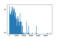
(a) Access counts

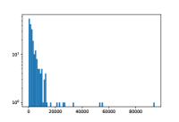
(b) Access sizes

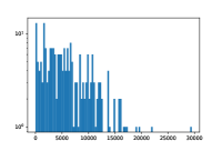
(c) Cache hit counts

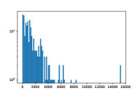
(d) Cache hit sizes

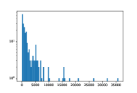
(e) Cache miss counts

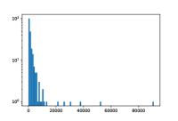
(f) Cache miss sizes

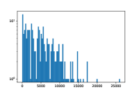
(g) Data reuse counts

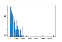
(h) Data reuse sizes

Figure 10. Distribution of daily features

4.1. LSTM on the Daily Data

We anticipate this modeling effort to be used in an advanced software-defined networking environment for possible resource allocation of a series of in-network caches. In this context, one useful time frame for considering possible resource allocation might be a few hours or a day. With this in mind, this work aggregates the cache utilization statistics into daily records. To construct this daily time series, we need to generate meaningful daily summaries along with other useful features that might support the prediction task. The daily summary of cache statistics includes the following features: (a) access counts, (b) access sizes, (c) cache hit counts, (d) cache hit sizes, (e) cache miss counts, (f) cache miss sizes, (g) data reuse counts, and (h) data reuse sizes.

Figure 10 shows the distribution of these daily summaries. Since these features have widely varying values, we plan to normalize these values before giving them to LSTM models. As there are many extreme values in the data, we have selected to use the z-score normalization (Saranya and Manikandan, 2013) instead of the more commonly used min-max normalization.

Due to the limited number of data points available, We allocate the data of the first 80% of the study period to be the training data, and the data of the last 20% of the study period to be the test data. The model selection would be based on how the model performs on the test data. The train dataset covers from July 1, 2021 to Dec. 16, 2021, and the test dataset covers from Dec. 19, 2021 to Jan. 29, 2022.

We prepared two different models, one with the above mentioned eight features and the second one with one additional feature, day-of-the-week. Because most workplaces follow the workweek schedule, we anticipate seeing a weekly trend and the day-of-the-week feature might improve the prediction accuracy. The day-of-the-week information is processed by one-hot encoding.

The input of the daily LSTM model is a vector of size 8 or 14, depending on whether day-of-the-week information is added. The first 8 are the normalized features of $N_{th}$ day, and the features include data access count, data access size, cache hit count, cache hit size, cache miss count, cache miss size, data reuse count, data reuse sizes. The last 6 are used for one-hot encoding representation of the day-of-the-week information, indicating whether of $N_{th}$ day is Monday to Saturday. If $N_{th}$ day is Sunday, then it’s represented as not Monday to Saturday.

The output of the LSTM model is a vector of size 8, the predicted normalized features of ${(N+1)}_{th}$ day, and the features include data access count, data access size, cache hit count, cache hit size, cache miss count, cache miss size, data reuse count, and data reuse sizes. The loss function is the root mean squared error (RMSE). All values in output vectors are given equal weights in calculating the loss.

Table 2. Hyper-parameters for Daily LSTM model

parameter	values
# of first layer LSTM unit	16, 32, 64, 128, 256
# of second layer LSTM unit	0, 16, 32, 64, 128, 256
first layer activation function	tanh, relu
second layer activation function	tanh, relu
dropout rate	0, 0.04, 0.1, 0.15
# of epochs	5, 10, 15, 25, 50, 75,100

Table 2 shows the 3360 combinations of hyper-parameters explored for tuning the daily LSTM model. As we have a limited number of data points, the explored models have a maximum of 2 LSTM layers, and each LSTM layer has a maximum of 256 LSTM units. The structure of the daily LSTM is shown in Figure 11a. When the number of the second layer LSTM unit is 0, the second LSTM layer does not exist; in this case, the daily LSTM is shown in Figure 11b. The hyper-parameter of the final daily LSTM model is chosen by the RMSE between the predicted test set values and the true test set values. The final model with the lowest RMSE for the test set is a 1-layer LSTM model shown in Figure 11b; its hyper-parameters are shown in table 3.

Table 3. hyper-parameter of the daily LSTM model

	# of LSTM unit	activation function	dropout rate	# of epochs
values	128	tanh	0.04	50

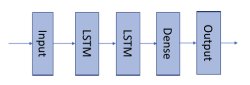
(a)

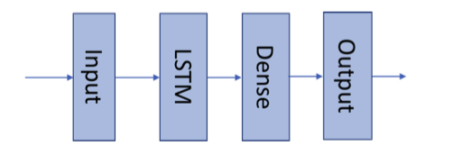
(b)

Figure 11. (a) 2-layer LSTM (b) 1-layer LSTM

Figure 12 shows how the daily LSTM model fits the daily access data. The model performs well when there are no extreme values, but as shown in Figure 12b, 12d, 12f, and 12h, the model does not fit and predict extreme values well. The gray shaded area is the predicted variance, defined as 2 standard deviations of the predicted values. If the actual value is within the predicted variance of the predicted value, we consider it as accurate. The overall accuracy is 0.884, and the accuracies for daily count data are all over 0.9.

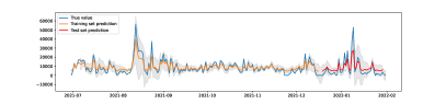
(a) Access counts

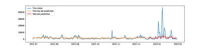
(b) Access sizes

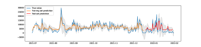
(c) Cache hit counts

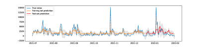
(d) Cache hit sizes

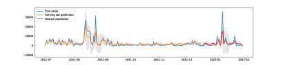
(e) Cache miss counts

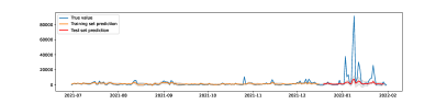
(f) Cache miss sizes

(g) Data reuse counts

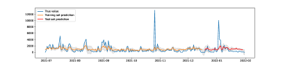
(h) Data reuse sizes

Figure 12. Daily LSTM model Train and Test result vs True Value

Table 4. RMSE of Daily LSTM model with and without using weekday information

	Without day-of-the-week		With day-of-the-week		Acc.
	Train RMSE	Test RMSE	Train RMSE	Test RMSE
Access Count	3,861.14	4,944.34	3,492.61	4,220.19	0.93
Access Size	2,480.61	16,621.57	2,612.90	16,571.21	0.85
Cache Hit Count	2,459.72	3,158.99	2,179.03	2,917.99	0.95
Cache Hit Size	1,425.66	2,144.92	1,375.42	2,154.87	0.85
Cache Miss Count	2,261.62	2,954.13	2,302.29	2,970.10	0.91
Cache Miss Size	1,265.84	17,324.68	1,298.15	16,426.95	0.90
Data Reuse Count	2,224.82	3,066.91	2,063.65	2,646.69	0.93
Data Reuse Size	1,135.80	1,482.21	1,099.14	1,466.38	0.73

Table 4 shows the RMSE of the Daily LSTM model on each daily data, along with the accuracy of the prediction. Note that the RMSE shown in this table is measured on the scale of the original values, not the normalized values. The overall accuracy is 0.884. The difference between the train RMSE and test RMSE on the size features is due to the model’s inability to fit on extreme values. When the day-of-the-week feature is added to the model for training, the model performance is improved on the daily counts, while the performance improvement in predicting daily sizes is minimal. The extreme values in the daily sizes make it hard to fit the daily sizes well; thus, adding day-of-the-week information can only improve the performance on the daily counts. This suggests that there might be a weekly seasonality in the daily data.

4.2. LSTM on the Daily Data with 7-Day Moving Average (MA LSTM Model)

In the previous study, we speculated that LSTM models perform poorly on the size feature because of the extreme values. To verify this claim, we have smoothed the daily summaries with a 7-day moving average.

The input and output of the MA LSTM model are a vector of size 8, the normalized features of $N_{th}$ day and ${(N+1)}_{th}$ day respectively, and the features include data access count, data access size, cache hit count, cache hit size, cache miss count, cache miss size, data reuse count, and data reuse sizes. The loss function is the root mean squared error (RMSE). All values in the output vectors are given equal weights in calculating the loss.

The same 3360 combinations of hyper-parameters shown in Table 2 are explored in the MA LSTM model. The model selection process is the same as the selection process for the daily LSTM model. The model with the lowest test RMSE is the 1-layer LSTM model shown in Figure 11b; its hyper-parameters are shown in Table 5. The hyper-parameters and constructions of the daily LSTM model and the MA LSTM model are very similar as they only differ in the dropout rate and the number of training epochs. This is due to the high similarity between the daily data and the daily data with 7-day moving average, and the limited number of available data points.

Table 5. hyper-parameter of the MA LSTM model

	# of LSTM unit	activation function	dropout rate	# of epochs
values	128	tanh	0.00	100

Figure 13 shows how the MA LSTM model fits the 7-day moving average on daily data. The model still deviates a lot on the extreme values in Figure 13f, but the model works well in general. The gray shaded area indicates the predicted variance, which is much smaller compared to the daily LSTM model.

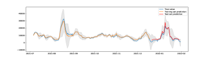
(a) Access counts

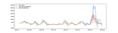
(b) Access sizes

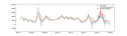
(c) Cache hit counts

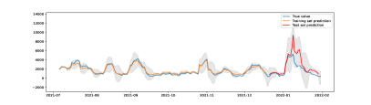
(d) Cache hit sizes

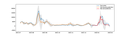
(e) Cache miss counts

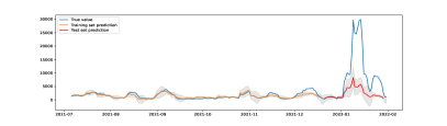
(f) Cache miss sizes

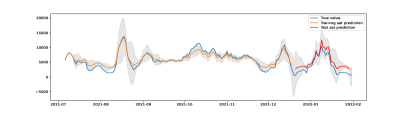
(g) Data reuse counts

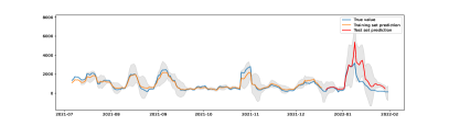
(h) Data reuse sizes

Figure 13. MA LSTM model Train and Test result vs True Value

Table 6. Explored Hyper-parameters for MA LSTM model

	Train RMSE	Test RMSE	Accuracy	Test RMSE reduction compare with daily LSTM
Access Count	1,122.15	2,169.72	0.93	48.6%
Access Size	744.56	7,729.04	0.83	53.4%
Cache Hit Count	829.23	2025.21	0.88	30.6%
Cache Hit Size	223.00	1,573.72	0.91	27.1%
Cache Miss Count	1,127.30	781.83	0.86	73.0%
Cache Miss Size	612.94	9616.83	0.77	58.5%
Data Reuse Count	808.80	1,228.71	0.87	53.6%
Data Reuse Size	208.27	812.33	0.92	44.6%

Table 6 shows the RMSE of the MA LSTM model, along with the prediction accuracy. Overall accuracy is 0.873. Although accuracy is less than 0.01 lower than the daily LSTM model, the predicted variance of the MA LSTM model is much smaller, so the prediction of the MA LSTM model is closer to the actual value. Compared to the RMSE of the daily LSTM model, the MA LSTM model performs much better overall in terms of the test set RMSE;

This shows that the LSTM model fits the daily data with 7-day moving average better than the daily data, which confirms that the extreme values severely affect the LSTM performance.

4.3. Seasonality

Day-of-the-week information improves the performance of the daily the LSTM model, which suggests some weekly seasonality in the daily time series data. We investigate the seasonality using periodograms (Shumway, Robert H and Stoffer, David S, 2017).

(a) Access counts

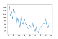
(b) Access sizes

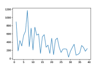
(c) Cache hit counts

(d) Cache hit sizes

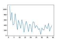
(e) Cache miss counts

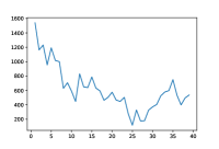
(f) Cache miss sizes

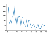
(g) Data reuse counts

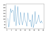
(h) Data reuse sizes

Figure 14. Periodogram of daily data. All eight features show the same peaks at 31 days and 62 days.

Figure 14 shows the periodogram of daily data. All columns show relatively strong, if not strongest, seasonal effects of 7 day period, confirming that there exists a weekly seasonal effect.

5. Conclusions

In this paper, we studied the access trends of the Southern California Petabyte Scale Cache operated by teams of high-energy physicists in California. Our analysis shows that the SoCal Repo was able to reduce the network traffic by 57% for a large portion of the period of the study. However, some periods of study show access patterns of streaming data which is an inefficient way of using the caching system, and impacts the performance of the backbone network. Through this study, we developed a number of machine learning models to further explore the predictability of the cache utilization statistics. Because the regional storage cache could predictably reduce the network utilization, we anticipate that a more general caching mechanism could benefit many more scientific communities beyond the specific physics community studied.

The study also reveals a number of unexpected characteristics worth further investigation. For example, the cache hit rates decrease significantly during the most recent months of the study, and a need for a larger dataset to train LSTM models.

- (1)
- Bauerdick et al. (2012) L Bauerdick, D Benjamin, K Bloom, B Bockelman, D Bradley, S Dasu, M Ernst, R Gardner, A Hanushevsky, H Ito, D Lesny, P McGuigan, S McKee, O Rind, H Severini, I Sfiligoi, M Tadel, I Vukotic, S Williams, F Würthwein, A Yagil, and W Yang. 2012. Using Xrootd to Federate Regional Storage. Journal of Physics: Conference Series 396, 4 (2012), 042009.
- Bauerdick et al. (2014) L. Bauerdick, K. Bloom, B. Bockelman, D. Bradley, S. Dasu, J. Dost, I. Sfiligoi, A. Tadel, M. Tadel, F. Wuerthwein, A. Yafil, and the CMS collaboration. 2014. XRootd, disk-based, caching proxy for optimization of data access, data placement and data replication. Journal of Physics: Conference Series 513, 4 (2014).
- Brown et al. (2020) Ben Brown, Eli Dart, Gulshan Rai, Lauren Rotman, and Jason Zurawski. 2020. Nuclear Physics Network Requirements Review Report. University of California, Publication Management System Report LBNL-2001281. Energy Sciences Network. https://www.es.net/assets/Uploads/20200505-NP.pdf
- Copps et al. (2021) E. Copps, H. Zhang, A. Sim, K. Wu, I. Monga, C. Guok, F. Wurthwein, D. Davila, and E. Fajardo. 2021. Analyzing scientific data sharing patterns with in-network data caching. In 4th ACM International Workshop on System and Network Telemetry and Analysis (SNTA 2021). ACM, ACM.
- Dorigo et al. (2005) A. Dorigo, P. Elmer, F. Furano, and A. Hanushevsky. 2005. XROOTD - A highly scalable architecture for data access. WSEAS Transactions on Computers 4, 4 (2005), 348–353.
- Espinal et al. (2020) X. Espinal, S. Jezequel, M. Schulz, A. Sciabà, I. Vukotic, and F. Wuerthwein. 2020. The Quest to solve the HL-LHC data access puzzle. EPJ Web of Conferences 245 (2020), 04027. https://doi.org/10.1051/epjconf/202024504027
- Fajardo et al. (2018) E. Fajardo, A. Tadel, M. Tadel, B. Steer, T. Martin, and F. Würthwein. 2018. A federated Xrootd cache. Journal of Physics: Conference Series 1085 (2018), 032025.
- Fajardo et al. (2020) Edgar Fajardo, Derek Weitzel, Mats Rynge, Marian Zvada, John Hicks, Mat Selmeci, Brian Lin, Pascal Paschos, Brian Bockelman, Andrew Hanushevsky, Frank Würthwein, and Igor Sfiligoi. 2020. Creating a content delivery network for general science on the internet backbone using XCaches. EPJ Web of Conferences 245 (2020), 04041. https://doi.org/10.1051/epjconf/202024504041
- Fajardo, Edgar et al. (2020) Fajardo, Edgar, Tadel, Matevz, Balcas, Justas, Tadel, Alja, Würthwein, Frank, Davila, Diego, Guiang, Jonathan, and Sfiligoi, Igor. 2020. Moving the California distributed CMS XCache from bare metal into containers using Kubernetes. EPJ Web Conf. 245 (2020), 04042. https://doi.org/10.1051/epjconf/202024504042
- Greff et al. (2016) Klaus Greff, Rupesh K Srivastava, Jan Koutník, Bas R Steunebrink, and Jürgen Schmidhuber. 2016. LSTM: A search space odyssey. IEEE transactions on neural networks and learning systems 28, 10 (2016), 2222–2232.
- Kalla and Sharma (2016) Anshuman Kalla and Sudhir Kumar Sharma. 2016. A constructive review of in-network caching: A core functionality of ICN. In 2016 International Conference on Computing, Communication and Automation (ICCCA). 567–574.
- Li et al. (2013) Yanhua Li, Haiyong Xie, Yonggang Wen, and Zhi-Li Zhang. 2013. Coordinating In-Network Caching in Content-Centric Networks: Model and Analysis. In 2013 IEEE 33rd International Conference on Distributed Computing Systems. 62–72. https://doi.org/10.1109/ICDCS.2013.71
- Pordes et al. (2007) Ruth Pordes, Don Petravick, Bill Kramer, Doug Olson, Miron Livny, Alain Roy, Paul Avery, Kent Blackburn, Torre Wenaus, Frank Würthwein, Ian Foster, Rob Gardner, Mike Wilde, Alan Blatecky, John McGee, and Rob Quick. 2007. The open science grid. Journal of Physics: Conference Series 78, 1 (2007), 012057.
- Rizzi, Andrea et al. (2019) Rizzi, Andrea, Petrucciani, Giovanni, and Peruzzi, Marco. 2019. A further reduction in CMS event data for analysis: the NANOAOD format. EPJ Web Conf. 214 (2019), 06021. https://doi.org/10.1051/epjconf/201921406021
- Saranya and Manikandan (2013) C Saranya and G Manikandan. 2013. A study on normalization techniques for privacy preserving data mining. International Journal of Engineering and Technology (IJET) 5, 3 (2013), 2701–2704.
- Sherstinsky (2020) Alex Sherstinsky. 2020. Fundamentals of recurrent neural network (RNN) and long short-term memory (LSTM) network. Physica D: Nonlinear Phenomena 404 (2020), 132306.
- Shumway, Robert H and Stoffer, David S (2017) Shumway, Robert H and Stoffer, David S. 2017. Time Series Analysis and Its Applications: With R Examples (4 ed.). Springer International Publishing AG. 166–172 pages.
- Sim et al. (2022) Alex Sim, Ezra Kissel, and Chin Guok. 2022. Deploying in-network caches in support of distributed scientific data sharing. https://doi.org/10.48550/ARXIV.2203.06843
- Weitzel et al. (2019) Derek Weitzel, Marian Zvada, Ilija Vukotic, Rob Gardner, Brian Bockelman, Mats Rynge, Edgar Hernandez, Brian Lin, and Mátyás Selmeci. 2019. StashCache: A Distributed Caching Federation for the Open Science Grid. PEARC ’19: Proceedings of the Practice and Experience in Advanced Research Computing on Rise of the Machines (learning), 1–7. https://doi.org/10.1145/3332186.3332212