Externally Valid Policy Choice

Abstract

We consider the problem of learning personalized treatment policies that are externally valid or generalizable: they perform well in other target populations besides the experimental (or training) population from which data are sampled. We first show that welfare-maximizing policies for the experimental population are robust to shifts in the distribution of outcomes (but not characteristics) between the experimental and target populations. We then develop new methods for learning policies that are robust to shifts in outcomes and characteristics. In doing so, we highlight how treatment effect heterogeneity within the experimental population affects the generalizability of policies. Our methods may be used with experimental or observational data (where treatment is endogenous). Many of our methods can be implemented with linear programming.

Keywords: Policy learning, Individualized treatment policies, External validity, Generalizability, Distributionally robust optimization, Optimal transport.

1 Introduction

There is increasing interest across many disciplines in personalized treatment policies. The typical objective is to choose a policy mapping individual characteristics into a treatment choice to maximize welfare. The maintained assumption underlying this literature is that the target population in which the policy is to be implemented is the same as the experimental (or training) population from which the data are sampled. While many policy learning algorithms have good welfare guarantees when the target and experimental populations are the same, the resulting policies can perform poorly in target populations that differ from the experimental population.

There are several reasons why the target and experimental populations may differ. Many of these mirror well known concerns about the external validity of experiments (see, e.g., BannerjeeDuflo2009; Deaton2010; Allcott2015). For instance, data may be collected under experimental conditions that differ from real-world settings in which the policy is to be implemented. Delays between data collection and policy implementation allow for the possibility that distributions may drift. The experiment may also define outcomes using easily measurable variables (e.g. test scores) while the policy maker may be concerned with more difficult to quantify outcomes (e.g. overall academic achievement). Experiments may also be run in selected sub-populations that are not representative of the broader target population.

We consider the problem of learning personalized treatment policies that are externally valid or generalizable: they perform well in other target populations besides the experimental population form which data are sampled. We allow for shifts in both the distribution of potential outcomes and characteristics between the experimental and target populations. We propose methods for learning externally valid policies using experimental or observational data (where treatment is possibly endogenous). Besides policy learning, our methods may be used as a stress test to assess the fragility or robustness of treatment policies to distributional shifts.

Consider a policy $\tau$ mapping individual characteristics $X$ into a binary outcome $\tau(X)$, where $\tau(X)=1$ indicates that treatment is to be assigned to an individual with characteristics $X$ and $\tau(X)=0$ indicates otherwise. Following Manski2004, policies are typically evaluated using a social welfare criterion

$$\mathrm{W}(\tau;P)=\mathbb{E}_{P}[Y_{1}\tau(X)+Y_{0}(1-\tau(X))]\,,$$ (1)

where $Y_{0}$ and $Y_{1}$ denote the individual’s untreated and treated potential outcomes, and $\mathbb{E}_{P}[\,\cdot\,]$ denotes expectation under the distribution $P$ of $(X,Y_{0},Y_{1})$ in the experimental population. It is also sometimes of interest to evaluate policies by their welfare gain relative to a policy in which no one is treated:

$$\mathrm{WG}(\tau;P) =\mathbb{E}_{P}[Y_{1}\tau(X)+Y_{0}(1-\tau(X))]-\mathbb{E}_{P}[Y_{0}]$$

$$=\mathbb{E}_{P}[(Y_{1}-Y_{0})\tau(X)]$$ (2)

The typical objective is to learn a policy that maximizes (1) or (2) over a class $\mathcal{T}$ that may incorporate functional-form, budget, fairness, or other constraints. The implicit assumption underlying this literature is that the experimental population is representative of the target population in which the policy is to be deployed.

Our objective is instead to derive generalizable policies that deliver uniform welfare guarantees over a set of target populations that are similar to, but different from, the experimental population. To this end, we replace criteria (1) and (2) with the robust welfare criterion

$$\mathrm{RW}(\tau;P)=\inf_{Q\in\mathcal{Q}}\mathrm{W}(\tau;Q)\,,$$ (3)

and the robust welfare gain criterion

$$\mathrm{RWG}(\tau;P)=\inf_{Q\in\mathcal{Q}}\mathrm{WG}(\tau;Q)\,,$$ (4)

respectively, where $\mathcal{Q}=\mathcal{Q}(P)$ is a set of target populations that are “close” to $P$ in a a very interpretable sense we make precise below. We propose methods to learn robust policies $\tau^{*}$ that maximize $\mathrm{RW}$ or $\mathrm{RWG}$ over $\mathcal{T}$. This max-min approach ensures that $\tau^{*}$ delivers welfare guarantees uniformly over all potential target populations $Q\in\mathcal{Q}$.

A novel aspect of our approach is to define $\mathcal{Q}$ using a class of Wasserstein metrics. This has several advantages. First, the size parameter $\varepsilon$ used to define $\mathcal{Q}$ is precisely the maximum that the average treatment effect (ATE) can differ between the experimental population $P$ and target populations $Q\in\mathcal{Q}$, as we show formally in Section 2. As such, the size of $\mathcal{Q}$ is very interpretable and may easily be calibrated by the analyst. Further, it serves as a unifying framework in which to study robustness to shifts in the distribution of potential outcomes only, and shifts in the distribution of both potential outcomes and characteristics. Wasserstein neighborhoods also lead to a tractable characterization of the robust welfare objectives (3) and (4).

Section 3 considers settings where the distribution of outcomes can shift between the experimental and target populations but the distribution of characteristics is held fixed. Propositions 3.1 and 3.2 characterize the robust welfare criterion (3) and robust welfare gain criterion (4) in this case. A number of implications are then explored. In particular, policies that are optimal under criteria (1) or (2) are also optimal under their robust counterparts (3) and (4). Further, policy learning methods with good regret guarantees under criteria (1) or (2), such as those proposed by Manski2004, QianMurphy2011, KitagawaTetenov2018, AtheyWager2021 and MTM, to name a few, also enjoy good regret guarantees under the corresponding robust criteria (3) or (4). We also show in Section 3.2 that these findings extend to settings with a known shift in characteristics.

Section 4 is concerned with shifts in both outcomes and characteristics between the experimental and target populations. We first derive the robust criteria (3) and (4) for this case in Propositions 4.1 and 4.2 then explore their implications. In particular, we show that both (i) the distribution of conditional average treatment effects (CATEs) and (ii) unobserved heterogeneity in treatment effects conditional on characteristics in the experimental population play distinct but important roles in shaping the external validity of treatment policies. By contrast, neither of these play a role in ranking policies under the usual criteria (1) and (2).

Section 4.3 discusses empirical implementation. Here the robust criteria depend on the joint distribution of characteristics and individual treatment effects in the experimental population. Because of the missing data problem, this distribution is not identified without further assumptions. We first derive sharp bounds on the robust welfare criterion in the absence of identifying assumptions. We then provide nonparametric estimators of the bounds and establish consistency and convergence rates. The bounds and their estimators are useful in their own right for assessing the fragility or robustness of policies to distribution shifts. Further, we provide a non-exhaustive set of methods for estimating robust policies under different identifying assumptions from the literature on distributional treatment effects (see, e.g., AbbringHeckman2007 and references therein) allowing experimental and observational data. We also provide convergence rates and regret guarantees for the estimated robust policies. Many of our methods can be implemented by linear programming.

We conclude in Section 5 with an empirical application that revisits the experiment of MKP2021 analyzing the effect of business training on rural Kenyan firms led by female entrepreneurs. Outcomes were measured over a four-year window following treatment, so there is a significant time lag between the experiment and any potential policy implementation. Our empirical findings reinforce some of the theoretical results we develop earlier about the role of heterogeneity in shaping generalizability. As a stress test, researchers could report plots similar to those we present in Section 5, which compare the robust welfare and robust welfare gain of different policies across different sized families of target populations.

Related Literature.

Like us, Kido2022, SZZB, and QiPangLiu2022 rank policies using a robust welfare criterion (3). These works and ours all use a different robustness set $\mathcal{Q}$ which leads to different rankings of policies. Kido2022 restricts the conditional distribution of outcomes given $X$ to Wasserstein neighborhoods (pointwise in $X$), and restricts the marginal distribution of $X$ to $f$-divergence (e.g., Kullback–Leibler divergence) neighborhoods. SZZB constrain the joint distribution of outcomes and $X$ to Kullback–Leibler neighborhoods. QiPangLiu2022 constrain the ratio of the densities in the experimental and target populations. Unlike Wasserstein neighborhoods, these constructions all prohibit extrapolation beyond the support of the experimental population, which may be restrictive in applications. The notion of neighborhood size is also more difficult to interpret for these constructions, whereas it has a clear interpretation in our setting. SZZB and QiPangLiu2022 study robustness with respect to shifts in the joint distribution of outcomes and $X$. Our paper and Kido2022 consider both joint shifts outcomes and $X$ as well as shifts in outcomes only. In the latter case, both produce the same ranking if outcomes are unbounded from below, but different rankings otherwise. Most importantly, none of these works shed light on how treatment effect heterogeneity within the experimental population affects generalizability.

MoQiLiu and Spini2021 seek individualized policies that are robust to shifts in the distribution of $X$ over $f$-divergence neighborhoods. A key and arguably very restrictive assumption underlying their approach is that the CATE does not change between the experimental and target populations. By contrast, we allow the CATE to shift between the two populations.

Similar to our paper, LSW2023 consider external validity of individualized treatment policies. They assume study participants are a non-random sample from the target population and model sampling bias, i.e., how participants select into the sample. Their robustness set $\mathcal{Q}$ consists of unknown target distributions that are consistent with the experimental population given selection. We instead do not take a stand on the cause of the shift between $P$ and $Q$, allowing for a general class of unstructured shifts in distributions.

Munro2023 considers individualized policies when agents strategically report their covariates. His paper also takes a position as to what causes the joint distribution to shift, namely strategic reporting by agents. This does not result in a distributionally robust problem; rather, the joint distribution of treatment effects and covariates in Munro2023 is a function of the policy. While we consider classes of deterministic policies, optimal policies with strategic agents may involve randomization.

2 Wasserstein Neighborhoods

In this section, we describe the set of target populations we work with and show that the neighborhood size has a clear interpretation as the maximal change in the ATE between the experimental and target populations.

Let $Z:=(X,Y_{0},Y_{1})$ take values in $\mathcal{Z}$ and let $d:\mathcal{Z}\times\mathcal{Z}\to\mathbb{R}_{+}\cup\{+\infty\}$ be a metric on $\mathcal{Z}$. The Wasserstein metric of order $p$ between $P$ and $Q$ is

$$d_{W,p}(P,Q)=\inf_{\pi\in\Pi(P,Q)}\mathbb{E}_{\pi}[d(Z,\tilde{Z})^{p}]^{\frac{1}{p}},\quad(1\leq p<\infty),$$

where $\Pi(P,Q)$ denotes all joint distributions for $(Z,\tilde{Z}$) with marginals $P$ for $Z$ and $Q$ for $\tilde{Z}$. We will focus on the metric with $p=1$, so we drop the $p$ subscript and write $d_{W}(P,Q)$ in what follows. This is mainly to simplify presentation: Appendix A discusses some generalizations to $p>1$.

We define Wasserstein neighborhoods using the metric

$$d((x,y_{0},y_{1}),(\tilde{x},\tilde{y}_{0},\tilde{y}_{1}))=|y_{0}-\tilde{y}_{0}|+|y_{1}-\tilde{y}_{1}|+b(x,\tilde{x}),$$ (5)

for a metric $b$. We use different choices of $b$ to handle robustness to shifts in outcomes only (as in Section 3) and shifts in outcomes and characteristics (as in Section 4).

We define neighborhoods as

$$\mathcal{Q}=\{Q:d_{W}(P,Q)\leq\varepsilon\},$$ (6)

where $\varepsilon>0$ is a measure of neighborhood size. As we now show, the parameter $\varepsilon$ is the maximum change in the ATE as $Q$ varies over $\mathcal{Q}$. This interpretation holds irrespective of whether we seek robustness with respect to shifts in outcomes only or outcomes and characteristics. First, we introduce some notation. Let $\mathcal{Y}$ denote the support of the potential outcomes, $\underline{Y}=\inf\mathcal{Y}$, and $\overline{Y}=\sup\mathcal{Y}$. For instance, $\mathcal{Y}=\{0,1\}$, $\underline{Y}=0$, and $\overline{Y}=1$ for binary outcomes, while $\mathcal{Y}=\mathbb{R}$, $\underline{Y}=-\infty$, and $\overline{Y}=+\infty$ if there are no restrictions on the support. We say that potential outcomes are unbounded if $\underline{Y}=-\infty$ or $\overline{Y}=+\infty$ (or both). Finally, let $\Delta=Y_{1}-Y_{0}$ denote the individual treatment effect.

Proposition 2.1

Suppose that $\mathcal{Q}$ is defined using $d_{W}(P,Q)$ induced by (5). Then

$$\inf_{Q\in\mathcal{Q}}\mathbb{E}_{Q}\left[\Delta\right] =\max\left\{\mathbb{E}_{P}\left[\Delta\right]-\varepsilon\,,\,\underline{Y}-\overline{Y}\right\},$$

$$\sup_{Q\in\mathcal{Q}}\mathbb{E}_{Q}\left[\Delta\right] =\min\left\{\mathbb{E}_{P}\left[\Delta\right]+\varepsilon\,,\,\overline{Y}-\underline{Y}\right\}.$$

If potential outcomes are unbounded, then

$$\inf_{Q\in\mathcal{Q}}\mathbb{E}_{Q}\left[\Delta\right] =\mathbb{E}_{P}\left[\Delta\right]-\varepsilon,$$ (7)

$$\sup_{Q\in\mathcal{Q}}\mathbb{E}_{Q}\left[\Delta\right] =\mathbb{E}_{P}\left[\Delta\right]+\varepsilon.$$

Remark 2.1

The bounds (7) apply for unbounded outcomes and also for bounded outcomes provided $\varepsilon$ is small enough that $\mathbb{E}_{P}[\Delta]$ is more than $\varepsilon$ from the trivial bounds $\underline{Y}-\overline{Y}$ and $\overline{Y}-\underline{Y}$. Moreover, these bounds are sharp: there exist distributions $Q\in\mathcal{Q}$ for which $\mathbb{E}_{Q}\left[\Delta\right]=\mathbb{E}_{P}\left[\Delta\right]\pm\varepsilon$. As such, Proposition 2.1 provides a formal sense in which the neighborhood size $\varepsilon$ is precisely the maximum that the ATE can vary between the experimental population $P$ and target populations $Q\in\mathcal{Q}$.

Remark 2.2

A similar argument to Proposition 2.1 shows that

$$\inf_{Q\in\mathcal{Q}}\mathbb{E}_{Q}\left[Y_{0}\right] =\max\left\{\mathbb{E}_{P}\left[Y_{0}\right]-\varepsilon\,,\,\underline{Y}\right\}, \sup_{Q\in\mathcal{Q}}\mathbb{E}_{Q}\left[Y_{0}\right] =\min\left\{\mathbb{E}_{P}\left[Y_{0}\right]+\varepsilon\,,\,\overline{Y}\right\}.$$

Hence, $\varepsilon$ can be calibrated from prior information on how average pretreatment outcomes differ between the experimental and target populations.

3 Shifts in Outcomes

In this section, we consider robustness with respect to shifts in the distribution of potential outcomes. This is relevant in a number of scenarios. First, it is relevant for designing policies to maximize welfare for the experimental population when welfare is defined using outcomes that are similar to, but possibly different from, outcomes that are measured in the experimental population. For instance, the policy maker may care about overall educational attainment, while the experiment measures outcomes in terms of a specific test score. It is also relevant when experimental conditions differ from the real-world setting in which the policy is to be implemented.

We start in Section 3.1 by introducing an appropriate neighborhood construction to handle this problem. Propositions 3.1 and 3.2 derive the robust criteria in this case. We then discuss several implications of these results. In particular, policies that are preferred under the social welfare criterion (1) or the welfare gain criterion (2) are also preferred under their robust counterparts. Hence, policy learning methods that have good guarantees under criteria (1) or (2) also enjoy good robustness guarantees with respect to shifts in outcomes. We then show in Section 3.2 that these findings extend to settings with known shifts in characteristics.

3.1 Robust Criteria

To allow for shifts in the distribution of potential outcomes while holding the distribution of characteristics fixed, we use Wasserstein divergence induced by the metric

$$d((x,y_{0},y_{1}),(\tilde{x},\tilde{y}_{0},\tilde{y}_{1}))=|y_{0}-\tilde{y}_{0}|+|y_{1}-\tilde{y}_{1}|+\infty\times\mathbb{I}[x\neq\tilde{x}].$$ (8)

This metric combines the $\ell^{1}$ norm to penalize the shifts in the distribution of outcomes and a discrete metric on the support $\mathcal{X}$ of $X$ to prohibit characteristic shifts.

The following result characterizes the robust welfare criterion. Recall that $\mathcal{Y}$ is the support of the potential outcomes, $\underline{Y}=\inf\mathcal{Y}$ and $\overline{Y}=\sup\mathcal{Y}$. We allow $\underline{Y}=-\infty$ and/or $\overline{Y}=+\infty$ in Propositions 3.1 and 3.2. To simplify the proofs in the case of unbounded outcomes, we assume that $\mathcal{Y}$ is equispaced, i.e., there is finite $C>0$ such that for any $y\in\mathcal{Y}$ the set $[y-C,y)\cap\mathcal{Y}$ is nonempty. Common supports such as $\mathbb{R}$, $\mathbb{R}_{+}$, $\mathbb{Z}$, and $\mathbb{Z}_{+}$ all satisfy this condition.

Proposition 3.1

Suppose that $\mathcal{Q}$ is defined using the Wasserstein metric $d_{W}(P,Q)$ induced by (8). Then for any policy $\tau$

$$\mathrm{RW}(\tau;P)=\max\Big{\{}\mathrm{W}(\tau;P)-\varepsilon\,,\,\underline{Y}\Big{\}}.$$

If potential outcomes are unbounded from below, then $\mathrm{RW}(\tau;P)=\mathrm{W}(\tau;P)-\varepsilon$.

An analogous result holds for robust welfare gain.

Proposition 3.2

Suppose that $\mathcal{Q}$ is defined using the Wasserstein metric $d_{W}(P,Q)$ induced by (8). Then for any policy $\tau$

$$\mathrm{RWG}(\tau;P)=\max\Big{\{}\mathrm{WG}(\tau;P)-\varepsilon\,,\,\mathbb{E}_{P}[\tau(X)](\underline{Y}-\overline{Y})\Big{\}}.$$

If potential outcomes are unbounded, then $\mathrm{RWG}(\tau;P)=\mathrm{WG}(\tau;P)-\varepsilon$.

Remark 3.1

Propositions 3.1 and 3.2 imply that any policy that maximizes criterion (1) or (2) must also maximize its robust counterpart (3) or (4), irrespective of the neighborhood size $\varepsilon$. Moreover, it follows from Proposition 3.1 that the regret of any estimated policy $\hat{\tau}$ under criterion (3) is bounded by its regret under criterion (1):

$$\sup_{\tau\in\mathcal{T}}\mathrm{RW}(\tau;P)-\mathrm{RW}(\hat{\tau};P)\leq\sup_{\tau\in\mathcal{T}}\mathrm{W}(\tau;P)-\mathrm{W}(\hat{\tau};P)\quad\mbox{for all $\varepsilon>0$.}$$

An analogous result holds for welfare gain. Hence, policy learning methods that have good (statistical) regret guarantees under criteria (1) or (2), such as those of Manski2004, QianMurphy2011, KitagawaTetenov2018, AtheyWager2021, and MTM, to name a few, also enjoy good regret guarantees under their robust counterparts (3) and (4).

Remark 3.2

When $\mathcal{Y}$ is a strict subset of $\mathbb{R}$, there may be many distributions $Q\in\mathcal{Q}$ under which the support of potential outcomes is different from $\mathcal{Y}$. This raises the concern that $\mathcal{Q}$ is “too large”, in the sense that it contains distributions with supports that the analyst would never confront in any realistic target population. The proof of Proposition 3.1 shows that if $\underline{Y}=-\infty$ or $\min\mathcal{Y}=\underline{Y}>-\infty$ hold, then the worst-case distributions that solve the minimization problem (3) have support $\mathcal{Y}$. An analogous result holds for welfare gain. The neighborhoods $\mathcal{Q}$ are therefore not too large, because the worst-case distributions that are being guarded against are precisely those that have support $\mathcal{Y}$.

3.2 Extension: Known Shifts in Characteristics

In some cases the analyst may be able to estimate (or have prior knowledge of) the distribution of characteristics in the target population. For instance, an experiment may sample one region but the analyst wishes to choose a policy for several neighboring regions. The distribution of characteristics in neighboring regions may be known e.g. from census or administrative data, and we might reasonably assume that the distribution of potential outcomes is similar, though not the same, across regions.

In this case, one could consider the re-weighted social welfare criterion

$$W_{\rho}(\tau;P)=\mathbb{E}_{P}\left[\left(Y_{1}\tau(X)+Y_{0}(1-\tau(X))\right)\rho(X)\right]$$ (9)

where $\rho(x)=q(x)/p(x)$ is the ratio of the marginal densities for $X$ in the target and experimental populations, respectively. This criterion was considered by KitagawaTetenov2018, UeharaKY20, and Kallus2021, amongst others, for policy learning under a known shift in characteristics. A similar weighting could be applied to the welfare gain criterion. These reweighted criteria are justified when the CATE is the same under $P$ and $Q$, in which case (9) corresponds to social welfare in population $Q$.

To study the implications of shifts in potential outcomes in this setting, consider

$$\inf_{Q\in\mathcal{Q}_{\rho}}W_{\rho}(\tau;Q)$$ (10)

where $\mathcal{Q}_{\rho}=\{Q:d_{W,\rho}(P,Q)\leq\varepsilon\}$ with

$$d_{W,\rho}(P,Q)=\inf_{\pi\in\Pi(P,Q)}\mathbb{E}_{\pi}[d(Z,\tilde{Z})\rho(X)]$$

for $Z=(X,Y_{0},Y_{1})$, and where $d$ is the metric (8). Criterion (10) gives robust welfare over distributions $Q$ in which $X$ has marginal density $q$ and the marginals for $Y_{0}$ and $Y_{1}$ are similar under $P$ and $Q$. An identical argument to Proposition 3.1 yields

$$\inf_{Q\in\mathcal{Q}_{\rho}}W_{\rho}(\tau;Q)=\max\left\{W_{\rho}(\tau;P)-\varepsilon\,,\,\underline{Y}\right\}.$$

The implications in Remark 3.1 also carry over to this re-weighted criterion. In particular, any policy that maximizes the re-weighted social welfare criterion (9) must also maximize its robust counterpart (10). An analogous result holds for welfare gain.

4 Shifts in Outcomes and Characteristics

We now turn to the problem of external validity when we allow for shifts in outcomes and characteristics. We begin in Section 4.1 by deriving the robust criteria, then explore their implications in Section 4.2. In particular, we show how the distribution of CATEs as well as unobserved heterogeneity in treatment effects conditional on characteristics (within the experimental population) play distinct but important roles in characterizing the external validity of treatment policies.

Section 4.3 discusses empirical implementation, allowing for experimental and observational data. Here the robust welfare criterion depends on joint distribution of characteristics and individual treatment effects in the experimental population. As this distribution is not identified without further assumptions, we first derive sharp bounds on robust welfare in the absence of identifying assumptions and show how the bounds can be estimated nonparametrically. We then provide approaches for estimating robust welfare under different identifying assumptions and establish convergence rates and regret guarantees for the estimated policies.

4.1 Robust Criteria

To allow for shifts in the distribution of potential outcomes and characteristics, we use Wasserstein divergence induced by the metric

$$d((x,y_{0},y_{1}),(\tilde{x},\tilde{y}_{0},\tilde{y}_{1}))=|y_{0}-\tilde{y}_{0}|+|y_{1}-\tilde{y}_{1}|+\|x-\tilde{x}\|,$$ (11)

where $\|\cdot\|$ is a norm on $\mathcal{X}$. We first derive the robust welfare criterion (3).

Proposition 4.1

Suppose that $\mathcal{Q}$ is defined using $d_{W}(P,Q)$ induced by (11) and that $\mathbb{E}_{P}[\|X\|]$ is finite. Then for any policy $\tau$,

$$\mathrm{RW}(\tau;P)=\max\left\{\sup_{\eta\geq 1}\mathbb{E}_{P}\left[\min\left\{Y_{0}+\eta h_{0}(X;\tau),Y_{1}+\eta h_{1}(X;\tau)\right\}\right]-\eta\varepsilon\,,\,\underline{Y}\right\},$$ (12)

where

$$h_{0}(x;\tau) =\inf_{\tilde{x}\in\mathcal{X}:\tau(\tilde{x})=0}\|x-\tilde{x}\|\,, h_{1}(x;\tau) =\inf_{\tilde{x}\in\mathcal{X}:\tau(\tilde{x})=1}\|x-\tilde{x}\|\,,$$

with the understanding that $h_{0}(x;\tau)=+\infty$ or $h_{1}(x;\tau)=+\infty$ if the infimum runs over an empty set. If potential outcomes are unbounded from below, then

$$\mathrm{RW}(\tau;P)=\sup_{\eta\geq 1}\mathbb{E}_{P}\left[\min\left\{Y_{0}+\eta h_{0}(X;\tau),Y_{1}+\eta h_{1}(X;\tau)\right\}\right]-\eta\varepsilon.$$

The first thing to note is the presence of the “$\min$” operation inside the expectation. This term follows from the interpretation of Lagrangian duality as a two-player zero-sum game. Fix any $(X,Y_{0},Y_{1})$ under $P$. Adversarial nature receives $-Y_{0}$ from shifting the individual to the non-treatment region at a cost of $\eta h_{0}(X;\tau)$ for a net gain of $-Y_{0}-\eta h_{0}(X;\tau)$. Similarly, $-Y_{1}-\eta h_{1}(X;\tau)$ is the net gain from shifting the individual to the treatment region. Nature chooses whichever is larger. Averaging across $P$ yields nature’s payoff, which is the negative of the expectation in (12).

The functions $h_{0}(x;\tau)$ and $h_{1}(x;\tau)$ represent the “distance to non-treatment” and “distance to treatment” under policy $\tau$ for an individual with characteristics $X=x$. Different policies $\tau$ induce different distances $h_{0}$ and $h_{1}$. For several popular classes of policies these distances have closed-form expressions or are otherwise efficient to compute. To simplify exposition, we take $\mathcal{X}=\mathbb{R}^{d}$ and let $\|\cdot\|$ be the Euclidean norm.

Example 4.1 (Linear Eligibility Score Policies)

Consider a policy of the form

$$\tau(x)=1\!\mathrm{l}\{\beta_{0}+x^{\prime}\beta_{1}\geq 0\}\,,$$

parameterized by $\beta_{0}$ (a scalar) and $\beta_{1}$ (a vector), where at least one element of $\beta_{1}$ is non-zero. The interpretation is that treatment is assigned when the eligibility score $x^{\prime}\beta_{1}$ exceeds the threshold $-\beta_{0}$. Here $h_{0}(x;\tau)$ and $h_{1}(x;\tau)$ are the minimum distances from $x$ to the half-spaces $\{\tilde{x}:\beta_{0}+\tilde{x}^{\prime}\beta_{1}\leq 0\}$ and $\{\tilde{x}:\beta_{0}+\tilde{x}^{\prime}\beta_{1}\geq 0\}$, namely

$$h_{0}(x;\tau)=\frac{(\beta_{0}+x^{\prime}\beta_{1})_{+}}{\|\beta_{1}\|},\quad\quad h_{1}(x;\tau)=\frac{(\beta_{0}+x^{\prime}\beta_{1})_{-}}{\|\beta_{1}\|},$$

where $(a)_{-}=-\min\{a,0\}$ and $(a)_{+}=\max\{a,0\}$.

Example 4.2 (Threshold Policies)

Consider a policy that assigns treatment when the values of certain characteristics are above or below given thresholds. For illustrative purposes we consider a policy that depends on the first two components of $X$:

$$\tau(x)=1\!\mathrm{l}\{s_{1}(x_{1}-\beta_{1})\geq 0\mbox{ and }s_{2}(x_{2}-\beta_{2})\geq 0\}$$

for $s_{1}=-1$ and $s_{2}=1$ and $\beta_{1},\beta_{2}\in\mathbb{R}$. Here $\tau(x)=1$ if and only if $x_{1}-\beta_{1}\leq 0$ and $x_{2}-\beta_{2}\geq 0$. Similarly, $\tau(x)=0$ if and only if $x_{1}-\beta_{1}<0$ or $x_{2}-\beta_{2}>0$. Hence,

$$h_{0}(x;\tau) =\sqrt{\min\left\{(x_{1}-\beta_{1})_{-}^{2}\,,(x_{2}-\beta_{2})_{+}^{2}\right\}}\,,$$

$$h_{1}(x;\tau) =\sqrt{(x_{1}-\beta_{1})_{+}^{2}+(x_{2}-\beta_{2})_{-}^{2}}\,.$$

Example 4.3 (Decision Trees)

Decision trees are defined by recursive partitions of $\mathcal{X}$ into regions for which the values of characteristics lie above or below given thresholds. Treatment is then assigned depending on whether characteristics lie in particular subsets of the resulting partition. Policies based on decision trees may be expressed as

$$\tau(x)=1\!\mathrm{l}\{x\in\cup_{k=1}^{K}C_{k}\}$$

where each $C_{k}$ is a hypercube. Different policies $\tau$ correspond to different sets $\cup_{k=1}^{K}C_{k}$. Note the non-treatment region $\mathcal{X}\setminus(\cup_{k=1}^{K}C_{k})$ is itself the union of finitely many nonempty hypercubes, say $\cup_{l=1}^{L}\tilde{C}_{l}$. The squared distance from $x$ to a hypercube $C$ is

$$\mathrm{dist}(x,C)^{2}=\min_{y}\|x-y\|^{2}\quad\mbox{subject to}\quad l_{i}\leq y_{i}\leq u_{i},\quad i=1,\ldots,d\,,$$

where $l_{i}$ and $u_{i}$, $i=1,\ldots,d$, define the boundaries of $C$ (we may have $l_{i}=-\infty$ or $u_{i}=+\infty$ for some $i$). Here $h_{0}(x;\tau)$ and $h_{1}(x;\tau)$ are then the minimum such distances from $x$ to the treatment and non-treatment hypercubes:

$$h_{0}(x;\tau)=\min_{1\leq k\leq K}\mathrm{dist}(x,C_{k})\,,\quad\quad h_{1}(x;\tau)=\min_{1\leq l\leq L}\mathrm{dist}(x,\tilde{C}_{l})\,.$$

Next, we derive the robust welfare gain criterion (4).

Proposition 4.2

Suppose that $\mathcal{Q}$ is defined using $d_{W}(P,Q)$ induced by (11) and that $\mathbb{E}_{P}[\|X\|]$ is finite. Then for any policy $\tau$,

$$\mathrm{RWG}(\tau;P)=\max\Bigg{\{}\sup_{\eta\geq 1}\mathbb{E}_{P}\left[\min\left\{\eta h_{0}(X;\tau),Y_{1}-Y_{0}+\eta h_{1}(X;\tau)\right\}\right]-\eta\varepsilon\,,\\ \sup_{\eta\in[0,1)}\mathbb{E}_{P}\left[\min\left\{\eta h_{0}(X;\tau),(1-\eta)(\underline{Y}-\overline{Y})+\eta(Y_{1}-Y_{0})+\eta h_{1}(X;\tau)\right\}\right]-\eta\varepsilon\Bigg{\}}.$$ (13)

If potential outcomes are unbounded, then

$$\mathrm{RWG}(\tau;P)=\sup_{\eta\geq 1}\mathbb{E}_{P}\left[\min\left\{\eta h_{0}(X;\tau),Y_{1}-Y_{0}+\eta h_{1}(X;\tau)\right\}\right]-\eta\varepsilon.$$

Remark 4.1

It follows from Propositions 4.1 and 4.2 that if potential outcomes are unbounded from below, we have

$$\mathrm{RW}(\tau;P)=\mathrm{RWG}(\tau;P)+\mathbb{E}_{P}[Y_{0}]\,.$$

Hence, in this case both robust criteria induce the same ordering over policies.

4.2 Implications

Before turning to empirical implementation, we first discuss some implications of the robust criteria derived in Propositions 4.1 and 4.2. In particular, we highlight different roles that treatment effect heterogeneity plays in the ranking of policies, and contrast this with the usual welfare criteria (1) and (2). We focus the following discussion on the robust welfare criterion from Proposition 4.1. In view of Remark 4.1, these findings carry over to the robust welfare gain criterion as well.

4.2.1 Heterogeneity in CATEs

Different patterns of heterogeneity in CATEs can have very different implications for the ranking of policies under distribution shifts. This is most easily seen when $\underline{Y}=-\infty$ and individual treatment effects $\Delta=Y_{1}-Y_{0}$ conditional on characteristics are constant, i.e., $\Delta|(X=x)=_{a.s.}\delta(x)$ holds for all $x$ under $P$. We emphasize that our methods do not require these assumptions; they are simply to facilitate the following discussion. Under these conditions, the social welfare criterion (1) becomes

$$\mathrm{W}(\tau;P)=\mathbb{E}_{P}[Y_{0}]+\mathbb{E}_{P}[\delta(X)|\tau(X)=1]P(\tau(X)=1)\,.$$

Consider ranking a policy $\tau$ relative to a policy in which no one is treated. As $P(\tau(X)=1)>0$, whether $\tau$ is preferred under criterion (1) is entirely determined by the sign of the average effect of treatment on the treated. In particular, the criterion is invariant to whether individuals with large negative treatment effects who are not treated under $\tau$ are “almost” treated in the sense that $h_{1}(X;\tau)$ is small. Similarly, it is invariant to whether treated individuals benefitting most from treatment are almost not treated. If so, such a policy may generalize poorly: there are distributions “close” to $P$ in which characteristics of a small mass of individuals with large negative or positive treatment effects are perturbed across the treatment/non-treatment frontier.

By constrast, the robust criterion from Proposition 4.1 becomes

$$\mathrm{RW}(\tau;P)=\mathbb{E}_{P}[Y_{0}]+\sup_{\eta\geq 1}\bigg{(}\mathbb{E}_{P}\left[\min\left\{\delta(X)+\eta h_{1}(X;\tau),0\right\}|\tau(X)=0\right]P(\tau(X)=0)\\ +\mathbb{E}_{P}\left[\min\left\{\eta h_{0}(X;\tau),\delta(X)\right\}|\tau(X)=1\right]P(\tau(X)=1)-\eta\varepsilon\bigg{)}\,.$$

Evidently, under the robust criterion both the sign of treatment effects for treated and non-treated individuals are taken into consideration, as are their magnitudes relative to how close the individuals are to the treatment/non-treatment frontier. “Robust” policies sort individuals by the size of their CATEs: individuals for whom $\delta(X)$ is small should be near the frontier, those for whom $\delta(X)$ is large should be far.

We illustrate this with a numerical example. Consider the two populations in Figure 1. In these populations, individual treatment effects (conditional on $(x_{1},x_{2})$) are constant so there is no unobserved heterogeneity. Individuals with $x_{1}+x_{2}\geq 0$ benefit from treatment whereas those with $x_{1}+x_{2}<0$ are adversely affected by it. In both populations the optimal policy $\tau^{opt}$ is to treat everyone with $x_{1}+x_{2}\geq 0$ and treat no one for whom $x_{1}+x_{2}<0$ (the frontier is represented by the dashed line). This policy generates the same social welfare in both populations:

$$\mathrm{W}(\tau^{opt};P_{a})=\mathrm{W}(\tau^{opt};P_{b})=1.5,$$

despite the fact that individuals for whom the treatment effect is largest are relatively far from the boundary between treatment/non-treatment in $P_{a}$ but near to it in $P_{b}$. Note that a policy that treats everyone $(\tau^{1})$ generates welfare $0.25$ (the ATE) in both populations whereas a policy that treats no one $(\tau^{0})$ generates zero welfare.

(a) Population $P_{a}$

(b) Population $P_{b}$

Figure 1: Two populations, different patterns of observable heterogeneity. Note: each number corresponds to a mass of individuals with the same characteristics $(x_{1},x_{2})$. The number represents the treated outcome $Y_{1}$, which is common to all individuals who share the same characteristics. All individuals in the population have $Y_{0}=0$. Individuals are uniformly distributed over the 12 mass points in each population.

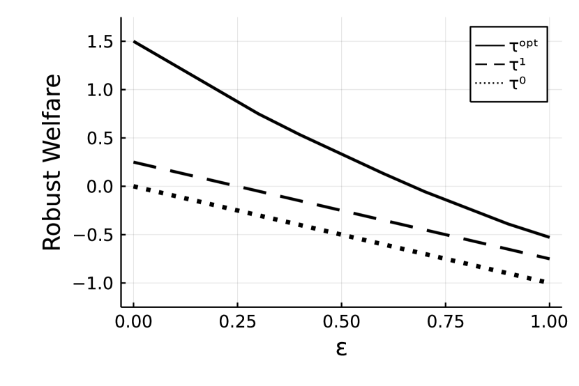
(a) Population $P_{a}$

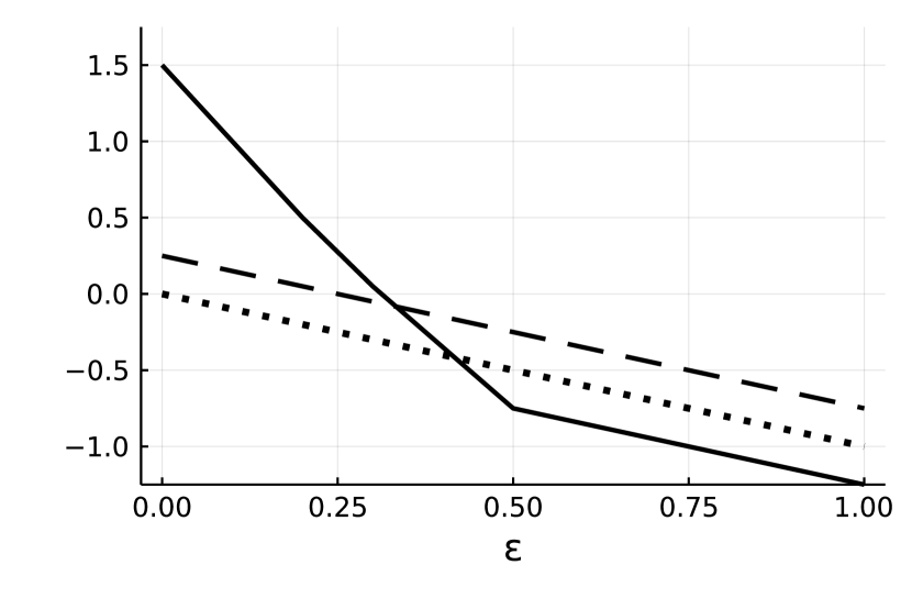
(b) Population $P_{b}$

Figure 2: Robust welfare in $P_{a}$ and $P_{b}$ as a function of neighborhood size $\varepsilon$.

Figure 2 plots the robust welfare of the policy $\tau^{opt}$ alongside the robust welfare of treating everyone ($\tau^{1})$ and no one ($\tau^{0}$) when $\underline{Y}=-\infty$. As $Y_{0}$ has mean zero and $\underline{Y}=-\infty$, the plots for $\tau^{opt}$ and $\tau^{1}$ also correspond to robust welfare gain (cf. Remark 4.1). To compute robust welfare, we take the six mass points closest to the boundary $x_{1}+x_{2}=0$ to be distance $1$ from the boundary, the next four mass points to be distance $2$, and the final two mass points to be distance $3$ from the boundary.

It is clear from Figure 2 that the performance of $\tau^{opt}$ is relatively insensitive to small perturbations of $P^{a}$. For instance with $\varepsilon=0.5$, which represents twice the ATE in $P_{a}$, robust welfare of $\tau^{opt}$ is positive and exceeds that of $\tau^{1}$ and $\tau^{0}$. By contrast, the ranking of the three policies changes in $P_{b}$ and $\tau^{opt}$ performs worse than both $\tau^{1}$ and $\tau^{0}$. For small $\varepsilon$, robust welfare of $\tau^{opt}$ decreases at a rate of 5 times neighborhood size in $P_{b}$, double the rate of decrease in $P_{a}$.

4.2.2 Unobserved Heterogeneity

A second important consequence of Proposition 4.1 is that unobserved heterogeneity in treatment effects now plays a role, whereas criterion (1) is invariant to unobserved heterogeneity. To see this, note that the inner expectation in the robust criterion (12) may be written

$$\mathbb{E}_{P}[Y_{0}]+\sup_{\eta\geq 1}\mathbb{E}_{P}\left[\min\left\{\Delta+\eta h_{1}(X;\tau),\eta h_{0}(X;\tau)\right\}\right]-\eta\varepsilon\,.$$ (14)

Consider populations $P_{c}$ and $P_{d}$ such that $(X,Y_{0})$ has the same distribution in both, but $\Delta|(X=x)=_{a.s.}\delta(x)$ holds for all $x$ in $P_{c}$ whereas $\mathbb{E}_{P_{d}}[\Delta|X=x]=\delta(x)$ in $P_{d}$. So, the conditional average treatment effects are the same for $P_{c}$ and $P_{d}$, but in $P_{d}$ there is unobserved heterogeneity whereas in $P_{c}$ there is none. It follows from expression (14) that

$$\mathrm{RW}(\tau;P_{c})\geq\mathrm{RW}(\tau;P_{d}),$$

where the inequality is strict if $\Delta$ has full support in $P_{d}$. The same is true for robust welfare gain. Intuitively, nature’s adversarial shifting of individuals into treatment or non-treatment regions concavifies the policy-maker’s utility function. Hence by Jensen’s inequality, robust welfare is lower when there is unobserved heterogeneity. This is in contrast to the usual criteria (1) and (2) which are invariant to unobserved heterogeneity:

$$\mathrm{W}(\tau;P_{c})=\mathrm{W}(\tau;P_{d})\,,\quad\quad\mathrm{WG}(\tau;P_{c})=\mathrm{WG}(\tau;P_{d})\,.$$

To see how unobserved heterogeneity plays a separate but distinct role from heterogeneity in CATEs, consider the population reported in Figure 1(a). Individual treatment effects are degenerate (conditional on characteristics) in this population. We construct alternative populations with unobserved heterogeneity in treatment effects by adding a mean-preserving spread of $\sigma W$ to individuals’ treated outcomes, where $\sigma\geq 0$ and $P(W=1)=P(W=-1)=\frac{1}{2}$. Note that in these populations the distribution of $X$ and CATEs are the same as Figure 1(a), all that changes is the variance of $Y_{1}$. Figure 3 plots the robust welfare (equivalently, robust welfare gain) of policies $\tau^{opt}$ as $\sigma$ varies over the grid $\{0,0.25,\ldots,3\}$. When $\varepsilon=0$, robust welfare is the same for all $\sigma$, reflecting the fact that the social welfare criterion (1) is invariant to unobserved heterogeneity. But as the degree of unobserved heterogeneity $\sigma$ and/or neighborhood size $\varepsilon$ increases, the robust welfare of the policy $\tau^{opt}$ is reduced to the point where $\tau^{opt}$ may no longer be favored over $\tau^{1}$ or even $\tau^{0}$.

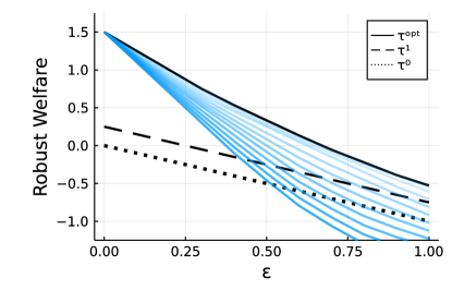
Figure 3: Robust welfare of policies for different values of the mean-preserving spread parameter $\sigma$. Note: black lines correspond to $\sigma=0$ (no unobserved heterogeneity), shaded lines to $\sigma\in\{0.25,0.5,\ldots,3\}$ (darker for more unobserved heterogeneity).

4.3 Empirical Strategies

We now present strategies for estimating externally valid policies given a finite data set drawn from the experimental population. The challenge as seen from (14) is that the criterion involves an expectation of a nonlinear function of individual treatment effects $\Delta=Y_{1}-Y_{0}$ in the experimental population $P$. Even in an experiment, the distribution of $(X,\Delta)$ is not identified without further assumptions. We first show how to estimate sharp bounds on robust welfare without further identifying assumptions. We then show how to estimate robust welfare under different identifying assumptions. For brevity we confine most of the discussion that follows to the robust welfare criterion, though this is not restrictive in view of Remark 4.1.

4.3.1 Sharp Bounds on Robust Welfare

In this section we derive sharp bounds on the robust criteria and show how they may be estimated. The bounds depend only on the joint distributions of $(X,Y_{0})$ and $(X,Y_{1})$ in the experimental population $P$. These two distributions are identified under the usual unconfoundedness (selection on observables) and overlap assumptions. They may also be identified from observational data under a variety of assumptions.

Our approach follows HeckmanSmithClements1997, Manski1997, and in particular FanPark2010 and Stoye2010 (see also ImbensMenzel2021). We seek to minimize and maximize $\mathrm{RW}(\tau;\tilde{P})$ over all distributions $\tilde{P}$ for which the marginals for $(X,Y_{0})$ and $(X,Y_{1})$ are the same as under $P$. Different couplings of the conditional distributions of $Y_{0}|X$ and $Y_{1}|X$ induce different distributions for $\Delta|X$. The expectation appearing in (14) may be written as

$$\mathbb{E}_{P}\left[\mathbb{E}_{P}\left[\left.\min\left\{\Delta+\eta h_{1}(X;\tau),\eta h_{0}(X;\tau)\right\}\right|X\right]\right].$$

The inner expectation is over a concave function of $\Delta$, so it suffices to consider second-order stochastic dominance (SSD) relations among distributions of $\Delta|X$ induced by different couplings. It is known from FanPark2010 that perfect positive dependence (or rank invariance) of $Y_{0}|X$ and $Y_{1}|X$ produces a distribution of $\Delta|X$ that SSDs all distributions of $\Delta|X$ induced by other couplings. Similarly, perfect negative dependence (or rank reversal) produces a distribution of $\Delta|X$ that is SSD by all distributions induced by other couplings. The upper bound on robust welfare is therefore achieved under perfect positive dependence while the lower bound is achieved under perfect negative dependence:

$$\mathrm{RW}(\tau;P^{-})\leq\mathrm{RW}(\tau;P)\leq\mathrm{RW}(\tau;P^{+})\quad\text{for all $\tau$},$$

where $P^{-}$ and $P^{+}$ denote the joint distribution of $(X,Y_{0},Y_{1})$ under perfect negative and positive dependence of $Y_{0}|X$ and $Y_{1}|X$, respectively, for $P$-almost every $X$. An analogous ranking holds for robust welfare gain:

$$\mathrm{RWG}(\tau;P^{-})\leq\mathrm{RWG}(\tau;P)\leq\mathrm{RWG}(\tau;P^{+})\quad\text{for all $\tau$}.$$

Remark 4.2

The upper bound under perfect positive dependence (or rank invariance) is interesting in two respects. First, if, as in the case of nonseparable models, rank invariance is a credible identifying assumption, then $P=P^{+}$ and $\mathrm{RW}(\tau;P)=\mathrm{RW}(\tau;P^{+})$ and $\mathrm{RWG}(\tau;P)=\mathrm{RWG}(\tau;P^{+})$ for all policies $\tau$. In this case, one can estimate policies that are robust to shifts in outcomes and characteristics by maximizing the empirical robust welfare criterion (18) introduced below or its modification for robust welfare gain.

The second use is as a stress test of a given policy, say $\hat{\tau}$: if the robust welfare (gain) of $\hat{\tau}$ under $P^{+}$ is bad, then robust welfare (gain) under $P$ must be even worse. The empirical robust welfare criterion (18) provides an estimate of $\mathrm{RW}(\hat{\tau};P^{+})$, which may be used to evaluate the robustness of estimated policies.

Remark 4.3

The lower bound is also interesting as it gives a welfare guarantee under both adversarial shifts between the experimental and target populations and adversarial couplings in the experimental population. The empirical robust welfare (gain) criterion under perfect negative dependence introduced below can be used to estimate robust policies which guard against both these adversaries.

Empirical Implementation.

Suppose we observe a random sample $(X_{i},Y_{i},D_{i})_{i=1}^{n}$, where $D_{i}$ is a binary treatment indicator, $Y_{i}=D_{i}Y_{1i}+(1-D_{i})Y_{0i}$, and the unconfoundedness condition

$$(Y_{0},Y_{1})\perp\!\!\!\perp D\,|\,X$$ (15)

and overlap condition

$$0<\Pr[D=1|X=x]<1\quad\mbox{for all $x\in\mathrm{supp}(P)$}$$ (16)

both hold. Then $F_{0}(y|x)=P(Y_{0}\leq y|X=x)$ and $F_{1}(y|x)=P(Y_{1}\leq y|X=x)$ are identified:

$$F_{d}(y|x)=\Pr(Y\leq y|X=x,D=d),\quad d=0,1.$$ (17)

Standard nonparametric methods can be used to estimate $F_{0}$ and $F_{1}$ based on (17). If unconfoundedness fails, then $F_{0}(y|x)$ and $F_{1}(y|x)$ may be identified using instrumental variables—see, e.g., VuongXu2017 and references therein.

To simplify exposition, suppose that $Y_{0}$ and $Y_{1}$ are continuously distributed conditional on $X$. Given $F_{0}$ and $F_{1}$, we may construct the counterfactual mappings

$$\phi_{x}^{+}(\cdot)=F_{1}^{-1}(F_{0}(\,\cdot\,|x)|x)\,,\quad\quad\phi_{x}^{-}(\cdot)=F_{1}^{-1}(1-F_{0}(\,\cdot\,|x)|x)\,.$$

The function $\phi_{x}^{+}$ maps an individual’s untreated outcome to their treated outcome under perfect positive dependence; its inverse maps treated outcomes to untreated outcomes. The function $\phi_{x}^{-}$ and its inverse give the same counterfactual mappings under perfect negative dependence. Individual $i$’s treatment effects under perfect positive and negative dependence are therefore

$$\Delta_{i}^{\!+} =D_{i}\left(Y_{i}-(\phi_{X_{i}}^{+})^{-1}(Y_{i})\right)+(1-D_{i})\left(\phi_{X_{i}}^{+}(Y_{i})-Y_{i}\right),$$

$$\Delta_{i}^{\!-} =D_{i}\left(Y_{i}-(\phi_{X_{i}}^{-})^{-1}(Y_{i})\right)+(1-D_{i})\left(\phi_{X_{i}}^{-}(Y_{i})-Y_{i}\right).$$

Given estimates $\hat{F}_{0}$ and $\hat{F}_{1}$, we may construct estimates $\hat{\phi}_{x}^{+}$ and $\hat{\phi}_{x}^{-}$ of $\phi_{x}^{+}$ and $\phi_{x}^{-}$. We may then estimate individual treatment effects under both dependence assumptions using

$$\hat{\Delta}_{i}^{\!+} =D_{i}\left(Y_{i}-(\hat{\phi}_{X_{i}}^{+})^{-1}(Y_{i})\right)+(1-D_{i})\left(\hat{\phi}_{X_{i}}^{+}(Y_{i})-Y_{i}\right),$$

$$\hat{\Delta}_{i}^{\!-} =D_{i}\left(Y_{i}-(\hat{\phi}_{X_{i}}^{-})^{-1}(Y_{i})\right)+(1-D_{i})\left(\hat{\phi}_{X_{i}}^{-}(Y_{i})-Y_{i}\right).$$

Finally, given an estimate $\bar{Y}_{0}$ of $\mathbb{E}_{P}[Y_{0}]$, we construct an empirical robust welfare criterion under perfect positive dependence as follows:

$$\mathrm{ERW}_{n}(\tau;P^{+})=\max\left\{\bar{Y}_{0}+\sup_{\eta\geq 1}\frac{1}{n}\sum_{i=1}^{n}\min\left\{\hat{\Delta}_{i}^{\!+}+\eta h_{1}(X_{i};\tau),\eta h_{0}(X_{i};\tau)\right\}-\eta\varepsilon\,,\,\underline{Y}\right\}.$$ (18)

The criterion $\mathrm{ERW}_{n}(\tau;P^{-})$ for perfect negative dependence is constructed analogously, replacing $\hat{\Delta}_{i}^{+}$ with $\hat{\Delta}_{i}^{-}$ in the above expression.

Remark 4.4

With unbounded outcomes, empirical robust welfare gain criteria under $P^{+}$ and $P^{-}$ can be constructed similarly by setting $\underline{Y}=-\infty$ and $\bar{Y}_{0}=0$ in (18). The results derived below in Propositions 4.3 and 4.4 apply equally to these criteria.

In practice, the optimization over $\eta$ may be efficiently performed using linear programming because for scalars $a_{i},b_{i},c_{i}$, $i=1,\ldots,n$, we have

$$\sup_{\eta\geq 1}\frac{1}{n}\sum_{i=1}^{n}\min\left\{a_{i}+b_{i},c_{i}\right\}-\eta\varepsilon =\sup_{\eta,(t_{i})_{i=1}^{n}}\frac{1}{n}\sum_{i=1}^{n}t_{i}-\eta\varepsilon,\quad\mbox{subject to}\quad\eta\geq 1,$$ (19)

$$\quad\quad t_{i}\leq a_{i}+b_{i},\quad t_{i}\leq c_{i},\quad i=1,\ldots,n.$$

Proposition 4.3

Suppose that the conditions of Proposition 4.1 hold, $\mathcal{X}$ is a bounded subset of $\mathbb{R}^{d}$, $\frac{1}{n}\sum_{i=1}^{n}|\hat{\Delta}^{\!+}_{i}-\Delta^{\!+}_{i}|\to_{p}0$, and $\bar{Y}_{0}\to_{p}\mathbb{E}_{P}[Y_{0}]$. Then

1. $\sup_{\tau\in\mathcal{T}}|\mathrm{ERW}_{n}(\tau;P^{+})-\mathrm{RW}(\tau;P^{+})|\to_{p}0$;

2. $\sup_{\tau\in\mathcal{T}}\mathrm{RW}(\tau;P^{+})-\mathrm{RW}(\hat{\tau};P^{+})\to_{p}0$ for any maximizer $\hat{\tau}$ of $\mathrm{ERW}_{n}(\,\cdot\,;P^{+})$.

Moreover, the convergence in parts 1. and 2. holds uniformly for $\varepsilon\geq\underline{\varepsilon}$ for any arbitrarily small $\underline{\varepsilon}>0$. An analogous result holds for $\mathrm{ERW}_{n}(\tau;P^{-})$.

Remark 4.5

Proposition 4.3 holds for any (and hence all) classes of policies $\mathcal{T}$. The price to pay for this generality is a bounded characteristic space $\mathcal{X}$, which is used to restrict the complexity of $\min\{\Delta^{\!\pm}+\eta h_{1}(X;\tau),\eta h_{0}(X;\tau)\}:\tau\in\mathcal{T}\}$. Only characteristics that are arguments of $\tau$ need to be bounded. If there are additional characteristics introduced, e.g., to ensure unconfoundedness is credibly satisfied but these characteristics do not appear as arguments of $\tau$, then they may be unbounded.

It is possible to relax boundedness of $\mathcal{X}$ and derive convergence rates under additional conditions on $\mathcal{T}$ and the estimators $\hat{\Delta}^{\!\pm}$ and $\bar{Y}_{0}$. Here we give one such result. Note one can identify each $\tau\in\mathcal{T}$ with a decision set $C$ such that $\tau(x)=\mathbb{I}[x\in C]$. Let $\mathcal{C}$ let the set of all decision sets as $\tau$ ranges over $\mathcal{T}$. A standard assumption in the econometrics literature on individualized treatment policies is that $\mathcal{C}$ is a VC class (i.e., has finite VC dimension), which means $\mathcal{T}$ has the same complexity as a parametric class. We impose a related condition. Let $\overline{C}$ denote the closure of a set $C$ and for $\delta\geq 0$ let $\overline{C}^{\delta}=\{x:\inf_{\tilde{x}\in\overline{C}}\|x-\tilde{x}\|\leq\delta\}$ denote its $\delta$-expansion. Let $\mathcal{C}^{c}=\{C^{c}:C\in\mathcal{C}\}$ and let $\mathcal{C}^{*}=\{\overline{C}^{\delta}:C\in\mathcal{C}\cup\mathcal{C}^{c},\delta\geq 0\}$. We require that $\mathcal{C}^{*}$ is a VC class, though we allow its VC dimension $v_{n}$ to grow with the sample size.

Proposition 4.4

Suppose that the conditions of Proposition 4.1 hold, $\mathbb{E}_{P}[Y_{d}^{2}]<\infty$ for $d=0,1$, $\mathcal{C}^{*}$ is a VC class of dimension $v_{n}$, and there are positive constants $a_{n},b_{n}$ such that $\frac{1}{n}\sum_{i=1}^{n}|\hat{\Delta}_{i}^{\!+}-\Delta_{i}^{\!+}|=O_{p}(a_{n})$ and $|\bar{Y}_{0}-\mathbb{E}_{P}[Y_{0}]|=O_{p}(b_{n})$. Then with $c_{n}=\max\{a_{n},b_{n},(v_{n}/n)^{1/2}\}$,

1. $\sup_{\tau\in\mathcal{T}}|\mathrm{ERW}_{n}(\tau;P^{+})-\mathrm{RW}(\tau;P^{+})|=O_{p}(c_{n})$;

2. $\sup_{\tau\in\mathcal{T}}\mathrm{RW}(\tau;P^{+})-\mathrm{RW}(\hat{\tau};P^{+})=O_{p}(c_{n})$ for any maximizer $\hat{\tau}$ of $\mathrm{ERW}_{n}(\,\cdot\,;P^{+})$.

Moreover, the convergence rates in parts 1. and 2. hold uniformly for $\varepsilon\geq 0$. An analogous result holds for $\mathrm{ERW}_{n}(\tau;P^{-})$.

Remark 4.6

The convergence rate $b_{n}$ will typically be $O(n^{-1/2})$, leading to an overall rate of $c_{n}=O(\max\{a_{n},(v_{n}/n)^{-1/2}\})$. We conjecture that it may be possible to reduce or remove the $a_{n}$ term to recover an $O((v_{n}/n)^{-1/2})$ rate (i.e., the minimax rate for welfare maximization over a VC class of policies of dimension $v_{n}$) using a doubly robust construction similar to that used by AtheyWager2021 for empirical welfare maximization. Unlike empirical welfare, here the nuisance parameter $\Delta$ enters the criterion non-smoothly. As this non-smooth problem appears to fall outside the scope of the current doubly/locally robust literature, we leave it for future work.

4.3.2 Identifying Assumption: No Unobserved Heterogeneity

A simple approach to identifying $P$ is to assume treatment effects are constant conditional on $X$, i.e.,

$$\Delta|(X=x)=_{a.s.}\delta(x)\,$$ (20)

for some function $\delta:\mathcal{X}\to\mathbb{R}$. Under this assumption, treatment effects can vary across individuals with different characteristics but are homogeneous for individuals with the same characteristics. While this assumption implies perfect positive dependence, it allows for easier empirical implementation as the problem of estimating the counterfactual mapping $\phi_{x}^{+}$ is replaced by the (simpler) problem of estimating $\delta$.

Empirical Implementation.

Suppose we observe a random sample $(X_{i},Y_{i},D_{i})_{i=1}^{n}$ where $D_{i}$ is a binary treatment indicator and $Y_{i}=D_{i}Y_{1i}+(1-D_{i})Y_{0i}$. Then $\delta$ is identified under the unconfoundedness condition (15) and the overlap condition (16). We may estimate $\delta$ using a variety of nonparametric regression techniques. Alternatively, suppose we observe $(X_{i},Y_{i},D_{i},Z_{i})_{i=1}^{n}$ where $Z_{i}$ is an instrumental variable satisfying appropriate regularity conditions (see, e.g., Abadie2003). By (20), $\delta$ is identified as the ratio

$$\delta(x)=\frac{\mathrm{Cov}(Y_{i},Z_{i}|X_{i}=x)}{\mathrm{Cov}(D_{i},Z_{i}|X_{i}=x)}$$

and may be estimated using nonparametric instrumental variables methods.

In either case, given estimators $\hat{\delta}$ of $\delta$ and $\bar{Y}_{0}$ of $\mathbb{E}_{P}[Y_{0}]$, we take $\hat{\Delta}_{i}\equiv\hat{\delta}(X_{i})$ to be our estimate of $\Delta_{i}\equiv\delta(X_{i})$ and form the empirical robust welfare criterion

$$\mathrm{ERW}_{n}(\tau;P)=\max\left\{\bar{Y}_{0}+\sup_{\eta\geq 1}\frac{1}{n}\sum_{i=1}^{n}\min\left\{\hat{\Delta}_{i}+\eta h_{1}(X_{i};\tau)\,,\eta h_{0}(X_{i};\tau)\right\}-\eta\varepsilon\,,\,\underline{Y}\right\}.$$

As before, the optimization over $\eta$ can be efficiently performed using linear programming (see equation (19)). We can estimate policies that are robust to shifts in outcomes and characteristics by maximizing this criterion with respect to $\tau\in\mathcal{T}$. Asymptotic properties of the estimated policy $\hat{\tau}$ may be established under a variety of regularity conditions. The following high-level results allow for both experimental and observational data.

Proposition 4.5

Suppose that the conditions of Proposition 4.1 hold, condition (20) holds, $\mathcal{X}$ is a bounded subset of $\mathbb{R}^{d}$, $\frac{1}{n}\sum_{i=1}^{n}|\hat{\Delta}_{i}-\Delta_{i}|\to_{p}0$, and $\bar{Y}_{0}\to_{p}\mathbb{E}_{P}[Y_{0}]$. Then

1. $\sup_{\tau\in\mathcal{T}}|\mathrm{ERW}_{n}(\tau;P)-\mathrm{RW}(\tau;P)|\to_{p}0$;

2. $\sup_{\tau\in\mathcal{T}}\mathrm{RW}(\tau;P)-\mathrm{RW}(\hat{\tau};P)\to_{p}0$ for any maximizer $\hat{\tau}$ of $\mathrm{ERW}_{n}(\,\cdot\,;P)$.

Moreover, the convergence in parts 1. and 2. holds uniformly for $\varepsilon\geq\underline{\varepsilon}$ for any arbitrarily small $\underline{\varepsilon}>0$.

For the next result, we again identify each $\tau\in\mathcal{T}$ with a decision set $C$ such that $\tau(x)=\mathbb{I}[x\in C]$ and impose a complexity condition from Section 4.3.1 on the sets.

Proposition 4.6

Suppose that the conditions of Proposition 4.1 hold, condition (20) holds, $\mathbb{E}_{P}[Y_{d}^{2}]<\infty$ for $d=0,1$, $\mathcal{C}^{*}$ is a VC class of dimension $v_{n}$, and there are positive constants $a_{n},b_{n}$ such that $\frac{1}{n}\sum_{i=1}^{n}|\hat{\Delta}_{i}-\Delta_{i}|=O_{p}(a_{n})$ and $|\bar{Y}_{0}-\mathbb{E}_{P}[Y_{0}]|=O_{p}(b_{n})$. Then with $c_{n}=\max\{a_{n},b_{n},(v_{n}/n)^{1/2}\}$,

1. $\sup_{\tau\in\mathcal{T}}|\mathrm{ERW}_{n}(\tau;P)-\mathrm{RW}(\tau;P)|=O_{p}(c_{n})$;

2. $\sup_{\tau\in\mathcal{T}}\mathrm{RW}(\tau;P)-\mathrm{RW}(\hat{\tau};P)=O_{p}(c_{n})$ for any maximizer $\hat{\tau}$ of $\mathrm{ERW}_{n}(\,\cdot\,;P)$.

Moreover, the convergence rates in parts 1. and 2. hold uniformly for $\varepsilon\geq 0$.

4.3.3 Identifying Assumption: Conditional Independence

An alternative identifying assumption is to posit the existence of a random variable $C$ such that all dependence between $Y_{0}$ and $Y_{1}$ given $X$ comes through $C$:

$$Y_{0}\perp\!\!\!\perp Y_{1}\,|\,X,C$$ (21)

(AbbringHeckman2007, Section 2.5.1), and that a suitably modified version of unconfoundedness holds:

$$(Y_{0},Y_{1})\perp\!\!\!\perp D\,|\,(X,C)\,.$$ (22)

The variables $C$ may correspond to those in $X$, but can be distinct. For example, $Y_{0}$ and $Y_{1}$ may be conditionally independent given $X$ and a latent common factor $F$, and $C$ could be a perfect proxy for $F$ constructed from $X$ and other observables. A special case are group fixed effects where potential outcomes (and possibly the assignment mechanism) has a group-specific component $\alpha_{C}$. Using a linear model for simplicity, we might have

$$Y_{0} =X^{\prime}\beta_{0}+\lambda_{0}\alpha_{C}+u_{0},$$

$$Y_{1} =X^{\prime}\beta_{1}+\lambda_{1}\alpha_{C}+u_{1},$$

with $C$ denoting the individual’s group membership (assumed known) and where $u_{0}$ and $u_{1}$ are conditionally independent given $(X,C)$.

Suppose the analyst observes a random sample $(X_{i},Y_{i},D_{i},C_{i})_{i=1}^{n}$ in which (21) and (22) hold and a suitably modified version of the overlap condition (16) holds. The conditional CDFs $F_{0}(\cdot|x,c)$ and $F_{1}(\cdot|x,c)$ are then nonparametrically identified as the conditional CDFs of $Y$ given $D=d,X=x,C=c$ for $d=0,1$, respectively. Assumption (21) then permits identification of the robust welfare criterion under $P$. Note the conditional CDF $G_{\eta,\tau}(\cdot|x,c)$ of $Z:=\min\left\{Y_{0}+\eta h_{0}(X;\tau)\,,Y_{1}+\eta h_{1}(X;\tau)\right\}$ given $X=x$ and $C=c$ is

$$G_{\eta,\tau}(z|x,c)=1-(1-F_{0}(z-\eta h_{0}(x;\tau)|x,c))(1-F_{1}(z-\eta h_{1}(x;\tau)|x,c)),$$

where $F_{0}$ and $F_{1}$ are the conditional CDFs of $Y_{0}$ and $Y_{1}$ given $X=x$ and $C=c$. It follows by iterated expectations that

$$\mathbb{E}_{P}\left[\min\left\{Y_{0}+\eta h_{0}(X;\tau)\,,Y_{1}+\eta h_{1}(X;\tau)\right\}\right]\\ =\int\int z\,\mathrm{d}G_{\eta,\tau}(z|x,c)\,\mathrm{d}P_{X,C}(x,c)\,,$$

where $P_{X,C}$ is the distribution of $(X,C)$ in the experimental population.

Given estimators $\hat{F}_{0}(y|x,c)$ and $\hat{F}_{1}(y|x,c)$, we estimate $G_{\eta,\tau}$ using

$$\hat{G}_{\eta,\tau}(z|x,c)=1-(1-\hat{F}_{0}(z-\eta h_{0}(x;\tau)|x,c))(1-\hat{F}_{1}(z-\eta h_{1}(x;\tau)|x,c))\,.$$

A nice feature of $\hat{G}_{\eta,\tau}$ is that it is uniformly consistent in $(z,\eta,\tau)$ whenever $\hat{F}_{0}(y|x,c)$ and $\hat{F}_{1}(y|x,c)$ are uniformly consistent in $y$. We choose $\hat{\tau}$ by maximizing the empirical robust welfare criterion

$$\mathrm{ERW}_{n}(\tau)=\max\left\{\sup_{\eta\geq 1}\frac{1}{n}\sum_{i=1}^{n}\int z\,\mathrm{d}\hat{G}_{\eta,\tau}(z|X_{i},C_{i})-\eta\varepsilon\,,\,\underline{Y}\right\}\,$$

with respect to $\tau\in\mathcal{T}$. The following result establishes consistency. Let $\bar{F}_{d}(y)=\frac{1}{n}\sum_{i=1}^{n}\hat{F}_{d}(y|X_{i},C_{i})$ for $d=0,1$, let $a,A$ be finite positive constants, and let wpa1 denote with probability approaching one.

Proposition 4.7

Suppose that the conditions of Proposition 4.1 hold, the conditional independence condition (21) holds, $\mathcal{X}$ is bounded, and $\int|y|^{1+a}\mathrm{d}\bar{F}_{d}(y)\leq A$ wpa1 and $\frac{1}{n}\sum_{i=1}^{n}\sup_{y}|\hat{F}_{d}(y|X_{i},C_{i})-F_{d}(y|X_{i},C_{i})|\to_{p}0$ for $d=0,1$. Then

1. $\sup_{\tau\in\mathcal{T}}|\mathrm{ERW}_{n}(\tau;P)-\mathrm{RW}(\tau;P)|\to_{p}0$;

2. $\sup_{\tau\in\mathcal{T}}\mathrm{RW}(\tau;P)-\mathrm{RW}(\hat{\tau};P)\to_{p}0$ for any maximizer $\hat{\tau}$ of $\mathrm{ERW}_{n}(\,\cdot\,;P)$.

Moreover, the convergence in parts 1. and 2. holds uniformly for $\varepsilon\geq\underline{\varepsilon}$ for any arbitrarily small $\underline{\varepsilon}>0$.

5 Empirical Illustration

We now present an application using data from MKP2021, who investigate the effect of the International Labour Organization’s Gender and Enterprise Together business training program on various outcomes (e.g., profits) for a sample of rural Kenyan firms run by female entrepreneurs. The training focuses on both standard business topics (e.g., record keeping, pricing) as well as topics designed to overcome gender constraints (e.g., division of household and business tasks). Firm outcomes are evaluated over a four-year window following training. Thus, there is a significant time lag between the experiment and any potential policy implementation, raising the possibility that distributions may drift.

The experiment used two layers of randomization: at the market level and again at the firm level. Markets were randomly assigned to treatment (at least one firm in the market is invited to training) or control (no firm is invited to training) conditional on strata. Strata were determined by geographic region and the number of firms in the market. Within treated markets, firms were randomly assigned treatment conditional on their baseline weekly profits reported in a pre-experiment market census. Thus, assignment is random conditional on both strata and baseline profits.

The outcome variable $Y$ is profits reported one year after training. To avoid issues of multi-valued treatments, we take the experimental population to be firms in treatment markets. We drop the few firms who do not report subsequent profits, leaving a sample of 2,009 firms, of which 1,096 are assigned treatment. The average treatment effect is approximately 157 Kenyan Shillings (KSh), roughly 11% of baseline profits.

We focus on a class of tree-based policies that assign treatment as a function of baseline profits (also measured in KSh). We consider trees of depth 2, so treatment is assigned depending on whether baseline profits lie in a certain interval. Within this class, the empirical welfare maximizing (EWM) policy is to treat if baseline profits exceed 40 KSh and are less than 3,034 KSh. Thus, only the very least and very most profitable firms are excluded from treatment under the EWM policy.

To examine the robustness of this policy to adversarial shifts in outcomes and baseline profits, we proceed as in Section 4.3.1 and estimate sharp bounds on robust welfare and robust welfare gain. We impute counterfactual mappings using kernel estimates of the distribution of treated and untreated outcomes conditional on strata and baseline earnings. We take $\underline{Y}=0$ as the post-treatment profit distribution appears truncated at zero, though quantitatively and qualitatively similar results are obtained with $\underline{Y}=-\infty$.

Figure 4 plots the upper bound on robust welfare and robust welfare gain for the EWM policy ($\tau^{\tiny\mbox{EWM}}$), policies in which all firms ($\tau^{1}$) or no firm ($\tau^{0}$) are/is treated, and some randomly selected parameterizations of tree policies. These upper bounds correspond to robust welfare and robust welfare gain if perfect positive dependence holds in the experimental population (cf. Remark 4.2). We plot over neighborhood sizes from $0$ to 100. For reference, the estimated ATE is 157 KSh, so the neighborhood size of 100 includes populations with an ATE between roughly 57 KSh and 257 KSh.

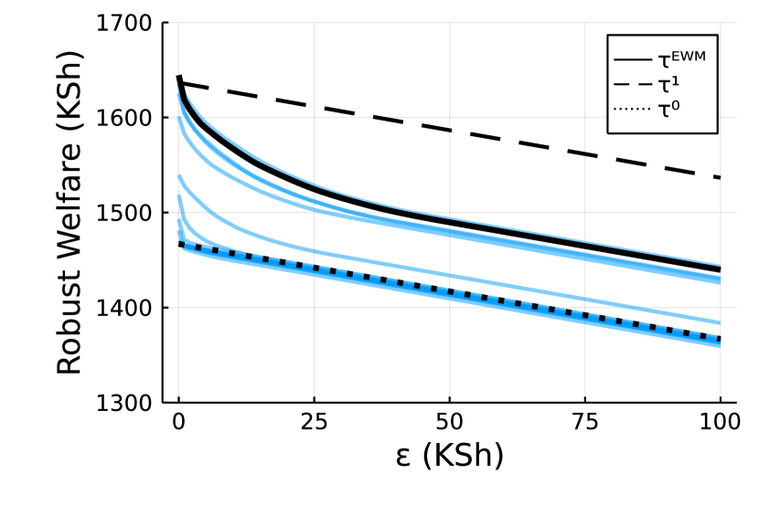
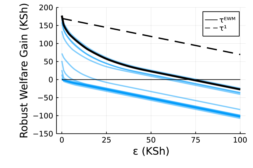
Figure 4: Robust welfare and welfare gain under perfect positive dependence. Note: $\tau^{\tiny\mbox{EWM}}$ is the EWM policy, $\tau^{1}$ and $\tau^{0}$ correspond to treating all firms and no firms, shaded lines correspond to some other parameterizations of tree policies.

The robust welfare of the EWM policy and many other individualized policies decays rapidly over small neighborhoods. For instance, with $\varepsilon=25$ KSh the robust welfare of the EWM policy is over 100 KSh below its welfare in the experimental population. Nevertheless, robust welfare of the EWM policy remains above all other parameterizations of tree policies and substantially above robust welfare of $\tau^{0}$ for all neighborhood sizes. Moreover, robust welfare gain is positive up to a neighborhood of size 70 or thereabouts, roughly 45% of the experimental population ATE. Thus, the EWM policy should deliver welfare improvements relative to treating no one, allowing for a broad class of distribution shifts. On the other hand, no individualized policy seems to deliver better robust welfare guarantees than a one-size-fits-all policy in which all firms are treated. As 98% of the experimental population are already treated under the EWM policy, the additional cost of treating the entire population seems small relative to the improvements in robust welfare.

To understand better why robust welfare decays rapidly, note there is substantial heterogeneity in individual treatment effects even under perfect positive dependence. The standard deviation of $\hat{\Delta}_{i}$ is approximately 706 KSh and the dispersion of $\hat{\Delta}_{i}$ appears independent of baseline profits. Hence, for any individualized policy, small adversarial shifts in baseline profits are sufficient push those near the boundary and who would benefit most from treatment into non-treatment regions and vice versa.

Lower bounds on robust welfare and robust welfare gain are plotted in Figure 5. Individual treatment effects are much more heterogeneous under perfect negative dependence: the standard deviation of $\hat{\Delta}_{i}$ is now approximately 3,225 KSh. In view of the discussion in Section 4.2, it is not surprising that robust welfare and welfare gain decay much faster. Indeed, the robust welfare gain of the EWM policy is only positive for $\varepsilon\leq 3$ KSh. For larger values of $\varepsilon$, individualized policies including the EWM policy all perform much worse than policies in which no one is treated. In all, these results suggest the EWM policy is preferred over $\tau^{0}$ and other tree policies if one wishes to guard against small distribution shifts. For robustness to larger distribution shifts, it seems preferable to adopt a policy in which training is provided to all firms.

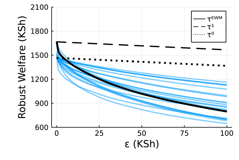
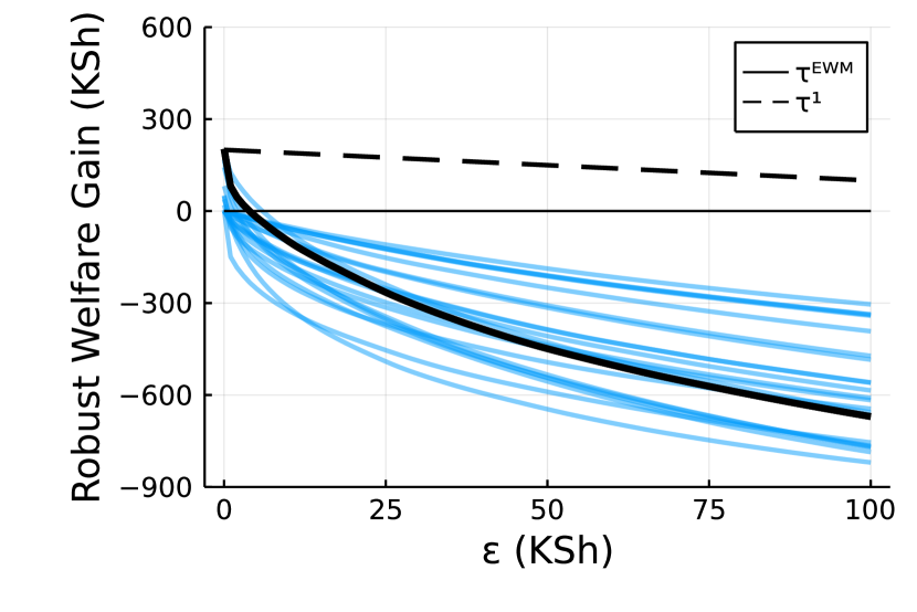
Figure 5: Robust welfare and welfare gain under perfect negative dependence. Note: $\tau^{\tiny\mbox{EWM}}$ is the EWM policy, $\tau^{1}$ and $\tau^{0}$ correspond to treating all firms and no firms, shaded lines correspond to some other parameterizations of tree policies.

6 Conclusion

We consider the problem of learning personalized treatment policies that perform well in target populations besides the experimental (or training) population from which data are sampled. Our main contribution is to develop new methods for policy learning that are robust to shifts in the distribution of both outcomes and characteristics between the experimental and target populations. In doing so, we shed light on how heterogeneity in CATEs and unobserved heterogeneity in treatment effects conditional on characteristics (within the experimental population) play distinct but important roles in characterizing the external validity of treatment policies. Besides policy learning, our methods may be used as a stress test to assess the fragility or robustness of treatment policies to distributional shifts.

Appendix A Other Wasserstein Metrics

Here we show that the conclusion of Proposition 3.1 is not specific to our choice of Wasserstein metric of order $1$. We focus on metrics of order $2$ as they are the most tractable; extensions to metrics of order $p$ is straightforward, but with more complicated notation. Let $\mathcal{Q}=\{Q:W_{2}(P,Q)\leq\varepsilon\}$ where $W_{2}(P,Q)$ is the Wasserstein metric of order 2 induced by

$$d((x,y_{0},y_{1}),(\tilde{x},\tilde{y}_{0},\tilde{y}_{1}))=\left(|y_{0}-\tilde{y}_{0}|^{2}+|y_{1}-\tilde{y}_{1}|^{2}+\infty\times\mathbb{I}[x\neq\tilde{x}]\right)^{1/2}.$$ (23)

The following result gives the robust welfare criterion (3) when $\mathcal{Y}=\mathbb{R}$.

Proposition A.1

Suppose that $\mathcal{Q}$ is defined using the Wasserstein metric $W_{2}(P,Q)$ induced by (23) and that $Y_{0}$ and $Y_{1}$ have finite second moments under $P$. Then for any policy $\tau$,

$$\inf_{Q\in\mathcal{Q}}\mathbb{E}_{Q}\left[Y_{1}\tau(X)+Y_{0}(1-\tau(X))\right]=\mathbb{E}_{P}[Y_{1}\tau(X)+Y_{0}(1-\tau(X))]-{\varepsilon}.$$

The robust welfare criterion in Proposition A.1 is the same as the criterion derived in Proposition 3.1 when $\underline{Y}=-\infty$. As such, Propositions 3.1 and A.1 provide a stronger sense in which policies with good guarantees under criterion (1) also have good external validity guarantees with respect to shifts in potential outcomes.

Appendix B General Consistency and Rate Results

We present here two general consistency and convergence rate results for the criterion

$$\mathrm{ERW}_{n}(\tau;P)=\max\left\{\bar{Y}_{0}+\sup_{\eta\geq 1}\frac{1}{n}\sum_{i=1}^{n}\min\left\{\hat{\Delta}_{i}+\eta h_{1}(X_{i};\tau),\eta h_{0}(X_{i};\tau)\right\}-\eta\varepsilon\,,\,\underline{Y}\right\},$$

with $P$ a generic experimental population and $\hat{\Delta}_{i}$ denoting an estimate of individual $i$’s treatment effect $\Delta_{i}$ under $P$, based on a random sample of size $n$ from the experimental population.

Proposition B.1

Suppose that the conditions of Proposition 4.1 hold, $\mathcal{X}$ is a bounded subset of $\mathbb{R}^{d}$, $\frac{1}{n}\sum_{i=1}^{n}|\hat{\Delta}_{i}-\Delta_{i}|\to_{p}0$, and $\bar{Y}_{0}-\mathbb{E}_{P}[Y_{0}]\to_{p}0$. Then

1. $\sup_{\tau\in\mathcal{T}}|\mathrm{ERW}_{n}(\tau;P)-\mathrm{RW}(\tau;P)|\to_{p}0$;

2. $\sup_{\tau\in\mathcal{T}}\mathrm{RW}(\tau;P)-\mathrm{RW}(\hat{\tau};P)\to_{p}0$ for any maximizer $\hat{\tau}$ of $\mathrm{ERW}_{n}(\,\cdot\,;P)$.

Moreover, the convergence in parts 1. and 2. holds uniformly for $\varepsilon\geq\underline{\varepsilon}$ for any arbitrarily small $\underline{\varepsilon}>0$.

Proposition B.2

Suppose that the conditions of Proposition 4.1 hold, $\mathbb{E}_{P}[Y_{d}^{2}]<\infty$ for $d=0,1$, $\mathcal{C}^{*}$ is a VC class of dimension $v_{n}$, and there are positive constants $a_{n},b_{n}$ such that $\frac{1}{n}\sum_{i=1}^{n}|\hat{\Delta}_{i}-\Delta_{i}|=O_{p}(a_{n})$ and $|\bar{Y}_{0}-\mathbb{E}_{P}[Y_{0}]|=O_{p}(b_{n})$. Then with $c_{n}=\max\{a_{n},b_{n},(v_{n}/n)^{1/2}\}$,

1. $\sup_{\tau\in\mathcal{T}}|\mathrm{ERW}_{n}(\tau;P)-\mathrm{RW}(\tau;P)|=O_{p}(c_{n})$;

2. $\sup_{\tau\in\mathcal{T}}\mathrm{RW}(\tau;P)-\mathrm{RW}(\hat{\tau};P)=O_{p}(c_{n})$ for any maximizer $\hat{\tau}$ of $\mathrm{ERW}_{n}(\,\cdot\,;P)$.

Moreover, the convergence rates in parts 1. and 2. hold uniformly for $\varepsilon\geq 0$.

Appendix C Proofs

Proof of Proposition 2.1. As $X$ does not appear in the objective, it is without loss of generality to drop characteristics by setting $b=0$ and letting $P$ and $Q$ be distributions over $(Y_{0},Y_{1})$. For brevity we just prove the lower bound. The Lagrangian is

$$L=\inf_{Q}\sup_{\eta\geq 0}\mathbb{E}_{Q}[Y_{1}-Y_{0}]+\eta(d_{W}(P,Q)-\varepsilon)\,.$$

The Lagrangian dual is

$$L^{\star} =\sup_{\eta\geq 0}\inf_{Q}\left(\mathbb{E}_{Q}[Y_{1}-Y_{0}]+\eta(d_{W}(P,Q)-\varepsilon)\right)$$

$$=\sup_{\eta\geq 0}\;\;\inf_{Q}\inf_{\pi\in\Pi(P,Q)}\mathbb{E}_{\pi}\bigg{[}\tilde{Y}_{1}-\tilde{Y}_{0}+\eta\left(|Y_{0}-\tilde{Y}_{0}|+|Y_{1}-\tilde{Y}_{1}|\right)\bigg{]}-\eta\varepsilon.$$

Note the iterated infimum over $Q$ and couplings $\pi\in\Pi(P,Q)$ is equivalent to infimizing over all joint distributions for $(Y_{0},Y_{1},\tilde{Y}_{0},\tilde{Y}_{1})$ with marginal $P$ for $(Y_{0},Y_{1})$. Hence,

$$L^{\star}=\sup_{\eta\geq 0}\inf_{\{F_{(\tilde{Y}_{0},\tilde{Y}_{1})|(Y_{0},Y_{1})}\}}\mathbb{E}_{P}\bigg{[}\mathbb{E}_{F_{(\tilde{Y}_{0},\tilde{Y}_{1})|(Y_{0},Y_{1})}}\bigg{[}\tilde{Y}_{1}-\tilde{Y}_{0}+\eta\left(|Y_{0}-\tilde{Y}_{0}|+|Y_{1}-\tilde{Y}_{1}|\right)\bigg{|}Y_{0},Y_{1}\bigg{]}\bigg{]}-\eta\varepsilon,$$

where the inf is over all conditional distribution for $(\tilde{Y}_{0},\tilde{Y}_{1})$ given $(Y_{0},Y_{1})$, for each $(Y_{0},Y_{1})$ in the support of $P$. As it is without loss of generality to optimize over point masses,

$$L^{\star}=\sup_{\eta\geq 0}\mathbb{E}_{P}\left[\inf_{\tilde{y}_{0},\tilde{y}_{1}}\left(\tilde{y}_{1}-\tilde{y}_{0}+\eta\left(|Y_{0}-\tilde{y}_{0}|+|Y_{1}-\tilde{y}_{1}|\right)\right)\right]-\eta\varepsilon.$$

For the inner problem, first suppose $\eta\in[0,1)$. Note $\tilde{y}_{1}+\eta|Y_{1}-\tilde{y}_{1}|$ is minimized by taking $\tilde{y}_{1}=\underline{Y}$. Similarly, $-\tilde{y}_{0}+\eta|Y_{0}-\tilde{y}_{0}|$ is minimized by taking $\tilde{y}_{0}=\overline{Y}$. Hence,

$$\mathbb{E}_{P}\left[\inf_{\tilde{y}_{0},\tilde{y}_{1}}\left(\tilde{y}_{1}-\tilde{y}_{0}+\eta\left(|Y_{0}-\tilde{y}_{0}|+|Y_{1}-\tilde{y}_{1}|\right)\right)\right]=(1-\eta)\left(\underline{Y}-\overline{Y}\right)+\eta\mathbb{E}_{P}[Y_{1}-Y_{0}]\,.$$

If $\eta\geq 1$, then $\tilde{y}_{1}+\eta|Y_{1}-\tilde{y}_{1}|$ is minimized by taking $\tilde{y}_{1}=Y_{1}$ and $-\tilde{y}_{0}+\eta|Y_{0}-\tilde{y}_{0}|$ is minimized by taking $\tilde{y}_{0}=Y_{0}$. Hence,

$$\mathbb{E}_{P}\left[\inf_{\tilde{y}_{0},\tilde{y}_{1}}\left(\tilde{y}_{1}-\tilde{y}_{0}+\eta\left(|Y_{0}-\tilde{y}_{0}|+|Y_{1}-\tilde{y}_{1}|\right)\right)\right]=\mathbb{E}_{P}[Y_{1}-Y_{0}]\,.$$

Combining the preceding three displays, we obtain $L^{\star}=\max\left\{\mathbb{E}_{P}[Y_{1}-Y_{0}]-\varepsilon\,,\,\underline{Y}-\overline{Y}\right\}$.

Finally, $L=L^{\star}$ follows by Theorem 1 of GaoKleywegt.    

Proof of Proposition 3.1. The Lagrangian and its dual are

$$L =\inf_{Q}\sup_{\eta\geq 0}\left(\mathbb{E}_{Q}[Y_{1}\tau(X)+Y_{0}(1-\tau(X))]+\eta(d_{W}(P,Q)-\varepsilon)\right),$$

$$L^{\star} =\sup_{\eta\geq 0}\inf_{Q}\left(\mathbb{E}_{Q}[Y_{1}\tau(X)+Y_{0}(1-\tau(X))]+\eta(d_{W}(P,Q)-\varepsilon)\right)$$

$$=\sup_{\eta\geq 0}\;\;\inf_{Q}\inf_{\pi\in\Pi(P,Q)}\mathbb{E}_{\pi}\bigg{[}\tilde{Y}_{1}\tau(\tilde{X})+\tilde{Y}_{0}(1-\tau(\tilde{X}))$$

$$\quad\quad\quad\quad\quad\quad\quad\quad+\eta\left(|Y_{0}-\tilde{Y}_{0}|+|Y_{1}-\tilde{Y}_{1}|+\infty\times\mathbb{I}[X\neq\tilde{X}]\right)\bigg{]}-\eta\varepsilon.$$

The inf over $Q$ and $\pi\in\Pi(P,Q)$ is equivalent to infimizing over all joint distributions for $(Z,\tilde{Z})$ with marginal $P$ for $Z$. It suffices to consider distribution for which $X=\tilde{X}$ almost surely. Hence,

$$L^{\star}=\sup_{\eta\geq 0}\inf_{\{F_{(\tilde{Y}_{0},\tilde{Y}_{1})|Z}\}}\mathbb{E}_{P}\bigg{[}\mathbb{E}_{F_{(\tilde{Y}_{0},\tilde{Y}_{1})|Z}}\bigg{[}\tilde{Y}_{1}\tau(X)+\tilde{Y}_{0}(1-\tau(X))\\ +\eta\left(|Y_{0}-\tilde{Y}_{0}|+|Y_{1}-\tilde{Y}_{1}|\right)\bigg{|}Z\bigg{]}\bigg{]}-\eta\varepsilon,$$

where the infimum is over all conditional distribution for $(\tilde{Y}_{0},\tilde{Y}_{1})$ given $Z$, for each $Z$ in the support of $P$. As it is without loss of generality to optimize over point masses,

$$L^{\star}=\sup_{\eta\geq 0}\mathbb{E}_{P}\left[\inf_{\tilde{y}_{0},\tilde{y}_{1}}\left(\tilde{y}_{1}\tau(X)+\tilde{y}_{0}(1-\tau(X))+\eta\left(|Y_{0}-\tilde{y}_{0}|+|Y_{1}-\tilde{y}_{1}|\right)\right)\right]-\eta\varepsilon.$$ (24)

The remainder of the proof will differ depending on whether $\underline{Y}>-\infty$ or $\underline{Y}=-\infty$.

Case 1: $\underline{Y}>-\infty$. The inner infimization with respect to $(\tilde{y}_{0},\tilde{y}_{1})$ in (24) may be solved in closed form for each fixed $Z=(X,Y_{0},Y_{1})$. Suppose $\eta\in[0,1)$. Then $y\mapsto y+\eta|Y-y|$ is minimized by setting $y=\underline{Y}$, with the minimizing value being $\underline{Y}+\eta(Y-\underline{Y})$. Therefore, the minimum is attained with $(\tilde{y}_{0},\tilde{y}_{1})=(Y_{0},\underline{Y})$ if $\tau(X)=1$ and $(\tilde{y}_{0},\tilde{y}_{1})=(\underline{Y},Y_{1})$ otherwise. For $\eta\in[0,1)$, the objective in (24) becomes

$$(1-\eta)\underline{Y}+\eta\left(\mathbb{E}_{P}\left[Y_{1}\tau(X)+Y_{0}(1-\tau(X))\right]-\varepsilon\right).$$

Maximizing with respect to $\eta\in[0,1)$ yields

$$\max\Big{\{}\mathbb{E}_{P}\left[Y_{1}\tau(X)+Y_{0}(1-\tau(X))\right]-\varepsilon\,,\,\underline{Y}\Big{\}}\,.$$

Conversely, if $\eta\geq 1$ then $y+\eta|Y-y|$ is minimized by setting $y=Y$, in which case the objective in (24) is $\mathbb{E}_{P}\left[Y_{1}\tau(X)+Y_{0}(1-\tau(X))\right]-\eta\varepsilon$, which is maximized with $\eta=1$. Combining these results yields $L^{\star}=\max\{\mathbb{E}_{P}\left[Y_{1}\tau(X)+Y_{0}(1-\tau(X))\right]-\varepsilon\,,\,\underline{Y}\}$.

It remains to show that $L=L^{\star}$. We provide a constructive proof. By weak duality ($L^{\star}\leq L$), it suffices to show $L\leq L^{\star}$. Partition $\mathcal{X}=\mathcal{X}_{0}\cup\mathcal{X}_{1}$ with $\mathcal{X}_{0}=\tau^{-1}(\{0\})$ and $\mathcal{X}_{1}=\tau^{-1}(\{1\})$. Let $Q_{0}$ denote the distribution of $T(Z)$ with $Z\sim P$, where

$$T(x,y_{0},y_{1})=\left\{\begin{array}[]{ll}(x,\underline{Y},y_{1})&\mbox{if $x\in\mathcal{X}_{0}$},\\ (x,y_{0},\underline{Y})&\mbox{if $x\in\mathcal{X}_{1}$}.\end{array}\right.$$

Then $\mathbb{E}_{Q_{0}}[Y_{1}\tau(X)+Y_{0}(1-\tau(X))]=\underline{Y}$. Consider the coupling $(Z,T(Z))\sim\pi$ for $Z\sim P$. Then under the metric (8), we have

$$d_{W}(P,Q_{0}) \leq\mathbb{E}_{\pi}[d((X,Y_{0},Y_{1}),(\tilde{X},\tilde{Y}_{0},\tilde{Y}_{1}))]$$

$$=\mathbb{E}_{P}[(Y_{0}-\underline{Y})\mathbb{I}[X\in\mathcal{X}_{0}]+(Y_{1}-\underline{Y})\mathbb{I}[X\in\mathcal{X}_{1}]]$$

$$=\mathbb{E}_{P}\left[Y_{1}\tau(X)+Y_{0}(1-\tau(X))\right]-\underline{Y}.$$ (25)

It follows that whenever $\mathbb{E}_{P}\left[Y_{1}\tau(X)+Y_{0}(1-\tau(X))\right]-\varepsilon<\underline{Y}$, we have

$$L\leq\sup_{\eta\geq 0}\left(\mathbb{E}_{Q_{0}}[Y_{1}\tau(X)+Y_{0}(1-\tau(X))]+\eta(d_{W}(P,Q_{0})-\varepsilon)\right)\\ \leq\underline{Y}+\sup_{\eta\geq 0}\eta\left(\mathbb{E}_{P}\left[Y_{1}\tau(X)+Y_{0}(1-\tau(X))\right]-\varepsilon-\underline{Y}\right)=L^{\star}.$$

If $\mathbb{E}_{P}\left[Y_{1}\tau(X)+Y_{0}(1-\tau(X))\right]-\varepsilon\geq\underline{Y}$, let $Q_{1}=wQ_{0}+(1-w)P$ be a mixture with

$$w=\frac{\varepsilon}{\mathbb{E}_{P}\left[Y_{1}\tau(X)+Y_{0}(1-\tau(X))\right]-\underline{Y}}\,.$$ (26)

Then $\mathbb{E}_{Q_{1}}[Y_{1}\tau(X)+Y_{0}(1-\tau(X))]=\mathbb{E}_{P}\left[Y_{1}\tau(X)+Y_{0}(1-\tau(X))\right]-\varepsilon$. Moreover, by convexity of $d_{W}$ (see, e.g., Villani (Villani, Theorem 4.8)),

$$d_{W}(P,Q_{1})\leq wd_{W}(P,Q_{0})+(1-w)d_{W}(P,P)=wd_{W}(P,Q_{0})\leq\varepsilon,$$

where the final equality follows from (25) and (26). Therefore, we again have

$$L\leq\sup_{\eta\geq 0}\left(\mathbb{E}_{Q_{1}}[Y_{1}\tau(X)+Y_{0}(1-\tau(X))]+\eta(d_{W}(P,Q_{1})-\varepsilon)\right)\\ \leq\mathbb{E}_{P}\left[Y_{1}\tau(X)+Y_{0}(1-\tau(X))\right]-\varepsilon+\sup_{\eta\geq 0}\eta(d_{W}(P,Q_{1})-\varepsilon)=L^{\star}.$$

Case 2: $\underline{Y}=-\infty$. Suppose $\eta\in[0,1)$. Then $y+\eta|Y-y|$ is minimized by taking $y\to-\infty$, and the minimizing value is $-\infty$. Conversely, if $\eta\geq 1$ then $y+\eta|Y-y|$ is minimized by setting $y=Y$, so the objective in (24) is $\mathbb{E}_{P}[Y_{0}+(Y_{1}-Y_{0})\tau(X)]-\eta\varepsilon$, which is maximized over $\eta\geq 1$ at $\eta=1$. Hence, $L^{\star}=\mathbb{E}_{P}\left[Y_{1}\tau(X)+Y_{0}(1-\tau(X))\right]-\varepsilon$.

It remains to show $L\leq L^{\star}$. As $\underline{Y}=-\infty$, for each $y$ we let $(y)_{\varepsilon}$ denote an element of $\mathcal{Y}$ for which $y-C\leq(y)_{\varepsilon}<y-\varepsilon$ for some constant $C>0$ (we can always choose such a $C$ and $(y)_{\varepsilon}$ because $\mathcal{Y}$ is be equispaced). Let $Q_{0}$ denote the distribution of $T(Z)$ with $Z\sim P$, where

$$T(x,y_{0},y_{1})=\left\{\begin{array}[]{ll}(x,(y_{0})_{\varepsilon},y_{1})&\mbox{if $x\in\mathcal{X}_{0}$},\\ (x,y_{0},(y_{1})_{\varepsilon})&\mbox{if $x\in\mathcal{X}_{1}$}.\end{array}\right.$$

Then

$$\mathbb{E}_{Q_{0}}[Y_{1}\tau(X)+Y_{0}(1-\tau(X))] =\mathbb{E}_{P}[(Y_{1})_{\varepsilon}\tau(X)+(Y_{0})_{\varepsilon}(1-\tau(X))]$$

$$<\mathbb{E}_{P}[Y_{1}\tau(X)+Y_{0}(1-\tau(X))]-\varepsilon\,,$$

where $\mathbb{E}_{Q_{0}}[Y_{1}\tau(X)+Y_{0}(1-\tau(X))]>\mathbb{E}_{P}[Y_{1}\tau(X)+Y_{0}(1-\tau(X))]-C$. Moreover, with $(Z,T(Z))\sim\pi$ for $Z\sim P$, we have

$$d_{W}(P,Q_{0}) \leq\mathbb{E}_{\pi}[d((X,Y_{0},Y_{1}),(\tilde{X},\tilde{Y}_{0},\tilde{Y}_{1}))]$$

$$=\mathbb{E}_{P}[(Y_{0}-(Y_{0})_{\varepsilon})\mathbb{I}[X\in\mathcal{X}_{0}]+(Y_{1}-(Y_{1})_{\varepsilon})\mathbb{I}[X\in\mathcal{X}_{1}]]$$

$$=\mathbb{E}_{P}\left[Y_{1}\tau(X)+Y_{0}(1-\tau(X))\right]-\mathbb{E}_{Q_{0}}[Y_{1}\tau(X)+Y_{0}(1-\tau(X))].$$ (27)

Let $Q_{1}=wQ_{0}+(1-w)P$ be a mixture distribution with weight

$$w=\frac{\varepsilon}{\mathbb{E}_{P}\left[Y_{1}\tau(X)+Y_{0}(1-\tau(X))\right]-\mathbb{E}_{Q_{0}}[Y_{1}\tau(X)+Y_{0}(1-\tau(X))]}$$ (28)

on $Q_{0}$. Then $\mathbb{E}_{Q_{1}}[Y_{1}\tau(X)+Y_{0}(1-\tau(X))]=\mathbb{E}_{P}\left[Y_{1}\tau(X)+Y_{0}(1-\tau(X))\right]-\varepsilon$. Moreover,

$$d_{W}(P,Q_{1})\leq wd_{W}(P,Q_{0})+(1-w)d_{W}(P,P)=wd_{W}(P,Q_{0})\leq\varepsilon,$$

by convexity of $d_{W}$ and (27) and (28). Therefore,

$$L\leq\sup_{\eta\geq 0}\left(\mathbb{E}_{Q_{1}}[Y_{1}\tau(X)+Y_{0}(1-\tau(X))]+\eta(d_{W}(P,Q_{1})-\varepsilon)\right)\\ \leq\mathbb{E}_{P}\left[Y_{1}\tau(X)+Y_{0}(1-\tau(X))\right]-\varepsilon+\sup_{\eta\geq 0}\eta(d_{W}(P,Q_{1})-\varepsilon)=L^{\star},$$

as required.    

Proof of Proposition 3.2. The proof is similar to the proof of Proposition 3.1.    

Proof of Proposition 4.1. We argue as for Proposition 3.1. The Lagrangian is

$$L=\inf_{Q}\sup_{\eta\geq 0}\left(\mathbb{E}_{Q}[Y_{1}\tau(X)+Y_{0}(1-\tau(X))]+\eta(d_{W}(P,Q)-\varepsilon)\right)$$

and its dual is

$$L^{\star}=\sup_{\eta\geq 0}\mathbb{E}_{P}\bigg{[}\inf_{(\tilde{x},\tilde{y}_{0},\tilde{y}_{1})}\bigg{(}\tilde{y}_{1}\tau(\tilde{x})+\tilde{y}_{0}(1-\tau(\tilde{x}))\\ +\eta\left(|Y_{0}-\tilde{y}_{0}|+|Y_{1}-\tilde{y}_{1}|+\|X-\tilde{x}\|\right)\bigg{)}\bigg{]}-\eta\varepsilon.$$ (29)

Consider the inner infimization at any fixed $Z=(X,Y_{0},Y_{1})$. We first fix $\tilde{x}$ and optimize with respect to $(\tilde{y}_{0},\tilde{y}_{1})$, then optimize with respect to $\tilde{x}$. There are two cases.

Case 1: $\underline{Y}>-\infty$. If $\eta\in[0,1)$, then the infimum with respect to $(\tilde{y}_{0},\tilde{y}_{1})$ (at fixed $\tilde{x}$) is attained with $(\tilde{y}_{0},\tilde{y}_{1})=(Y_{0},\underline{Y})$ when $\tau(\tilde{x})=1$ and $(\tilde{y}_{0},\tilde{y}_{1})=(\underline{Y},Y_{1})$ when $\tau(\tilde{x})=0$. For $\eta\in[0,1)$, the objective in (29) becomes

$$(1-\eta)\underline{Y}+\eta\mathbb{E}_{P}\left[Y_{0}+\inf_{\tilde{x}}\left((Y_{1}-Y_{0})\tau(\tilde{x})+\|X-\tilde{x}\|\right)\right]-\eta\varepsilon.$$

Maximizing with respect to $\eta\in[0,1)$ yields

$$\max\left\{\mathbb{E}_{P}\left[Y_{0}+\inf_{\tilde{x}}\left((Y_{1}-Y_{0})\tau(\tilde{x})+\|X-\tilde{x}\|\right)\right]-\varepsilon,\underline{Y}\right\}.$$

If $\eta\geq 1$, then the infimum with respect to $(\tilde{y}_{0},\tilde{y}_{1})$ (at fixed $\tilde{x}$) is attained with $(\tilde{y}_{0},\tilde{y}_{1})=(Y_{0},Y_{1})$ and the objective in (29) becomes

$$\mathbb{E}_{P}\left[Y_{0}+\inf_{\tilde{x}}\left((Y_{1}-Y_{0})\tau(\tilde{x})+\eta\left(\|X-\tilde{x}\|\right)\right)\right]-\eta\varepsilon.$$ (30)

Case 2: $\underline{Y}=-\infty$. If $\eta\in[0,1)$, then the infimum is achieved by taking $\tilde{y}_{0}\to-\infty$ and/or $\tilde{y}_{1}\to-\infty$ and the infimum is again attained with $(\tilde{y}_{0},\tilde{y}_{1})=(Y_{0},Y_{1})$ minimizing value is $-\infty$. Conversely if $\eta\geq 1$ then the infimum is attained with $(\tilde{y}_{0},\tilde{y}_{1})=(Y_{0},Y_{1})$ and the dual objective again reduces to (30).

Combining these results, we obtain

$$L^{\star}=\max\left\{\sup_{\eta\geq 1}\mathbb{E}_{P}\left[Y_{0}+\inf_{\tilde{x}}\left((Y_{1}-Y_{0})\tau(\tilde{x})+\eta\|X-\tilde{x}\|\right)\right]-\eta\varepsilon\,,\,\underline{Y}\right\}.$$

We may split the infimization up into separate infimizations over $\{\tilde{x}:\tau(\tilde{x})=0\}$ and $\{\tilde{x}:\tau(\tilde{x})=1\}$, then take the minimum:

$$L^{\star} =\max\left\{\sup_{\eta\geq 1}\mathbb{E}_{P}\left[Y_{0}+\min\left\{Y_{1}-Y_{0}+\inf_{\tilde{x}:\tau(\tilde{x})=1}\eta\|X-\tilde{x}\|,\inf_{\tilde{x}:\tau(\tilde{x})=0}\eta\|X-\tilde{x}\|\right\}\right]-\eta\varepsilon\,,\,\underline{Y}\right\}$$

$$=\max\left\{\sup_{\eta\geq 1}\mathbb{E}_{P}\left[Y_{0}+\min\left\{Y_{1}-Y_{0}+\eta h_{1}(X;\tau),\eta h_{0}(X;\tau)\right\}\right]-\eta\varepsilon\,,\,\underline{Y}\right\}\,.$$

Finally, strong duality holds by Theorem 1 of GaoKleywegt.    

Proof of Proposition 4.2. We argue as in the proof of Proposition 4.1, stating only the necessary modifications. The dual is

$$L^{\star}=\sup_{\eta\geq 0}\mathbb{E}_{P}\bigg{[}\inf_{(\tilde{x},\tilde{y}_{0},\tilde{y}_{1})}\bigg{(}(\tilde{y}_{1}-\tilde{y}_{0})\tau(\tilde{x})+\eta\left(|Y_{0}-\tilde{y}_{0}|+|Y_{1}-\tilde{y}_{1}|+\|X-\tilde{x}\|\right)\bigg{)}\bigg{]}-\eta\varepsilon.$$ (31)

Case 1: bounded outcomes. If $\eta\in[0,1)$, then the infimum with respect to $(\tilde{y}_{0},\tilde{y}_{1})$ (at fixed $\tilde{x}$) is attained with $(\tilde{y}_{0},\tilde{y}_{1})=(\overline{Y},\underline{Y})$ if $\tau(\tilde{x})=1$ and $(\tilde{y}_{0},\tilde{y}_{1})=(Y_{0},Y_{1})$ if $\tau(\tilde{x})=0$. For $\eta\in[0,1)$, the objective in (31) becomes

$$\mathbb{E}_{P}\left[\inf_{\tilde{x}}\left(\tau(\tilde{x})(\underline{Y}-\overline{Y}+\eta(\overline{Y}-Y_{0})+\eta(Y_{1}-\underline{Y}))+\eta\|X-\tilde{x}\|\right)\right]\\ =\mathbb{E}_{P}\left[\min\left\{(1-\eta)(\underline{Y}-\overline{Y})+\eta(Y_{1}-Y_{0})+\eta h_{1}(X;\tau),\eta h_{0}(X;\tau)\right\}\right]\,.$$

If $\eta\geq 1$ then the infimum is achieved with $(\tilde{y}_{0},\tilde{y}_{1})=(Y_{0},Y_{1})$ and the objective in (31) becomes

$$\mathbb{E}_{P}\left[\inf_{\tilde{x}}\left(\tau(\tilde{x})(Y_{1}-Y_{0})+\eta\|X-\tilde{x}\|\right)\right]\\ =\mathbb{E}_{P}\left[\min\left\{(Y_{1}-Y_{0})+\eta h_{1}(X;\tau),\eta h_{0}(X;\tau)\right\}\right]\,.$$ (32)

Case 2: unbounded outcomes. If $\eta\in[0,1)$, then the minimum is achieved by setting $\tilde{y}_{0}\to+\infty$ if $\overline{Y}=+\infty$ and/or $\tilde{y}_{1}\to-\infty$ if $\underline{Y}=-\infty$ for any $\tilde{x}$ for which $\tau(\tilde{x})=1$. Hence, the objective in (31) is $-\infty$ for $\eta\in[0,1)$ for any policy $\tau$ for which $\tau(x)=1$ for some $x$, and is zero otherwise. Conversely if $\eta\geq 1$ then the minimum is achieved with $(\tilde{y}_{0},\tilde{y}_{1})=(Y_{0},Y_{1})$ and the objective reduces to (32).

Strong duality again holds by Theorem 1 of GaoKleywegt.    

Proof of Propositions 4.3 and 4.4. Immediate from Propositions B.1 and B.2, setting $P=P^{\pm}$ and $\Delta=\Delta^{\pm}$.    

Proof of Propositions 4.5 and 4.6. Immediate from Propositions B.1 and B.2, invoking (20) and setting $\Delta=\delta(X)$.    

Proof of Proposition 4.7. We proceed as in the proof of Propositions 4.3 and 4.5. To simplify notation, let $\hat{G}^{(i)}_{\eta,\tau}(z)=\hat{G}_{\eta,\tau}(z|X_{i},C_{i})$, and similarly for $G_{\eta,\tau}$, $\hat{F}_{0}$, $\hat{F}_{1}$, $F_{0}$, and $F_{1}$. By the functional form of $\mathrm{RW}_{n}$, it suffices to show

$$\sup_{\tau\in\mathcal{T}}\bigg{|}\sup_{\eta\geq 1}\bigg{(}\frac{1}{n}\sum_{i=1}^{n}\int z\,\mathrm{d}\hat{G}_{\eta,\tau}^{(i)}(z)-\eta\varepsilon\bigg{)}\\ -\bigg{(}\sup_{\eta\geq 1}\int\int z\,\mathrm{d}G_{\eta,\tau}(z|x,c)\,\mathrm{d}P_{X,C}(x,c)-\eta\varepsilon\bigg{)}\bigg{|}=o_{p}(1).$$

We first show that there is a sufficiently large constant $B$ such that for all $\tau\in\mathcal{T}$, the argsup of both problems is an element of $[1,B]$ wpa1. For the first problem, suppose the assertion is false. Then for some $\tau\in\mathcal{T}$, $\eta\geq B$, and $\varepsilon\geq\underline{\varepsilon}$, we have

$$\frac{1}{n}\sum_{i=1}^{n}\int z\,\mathrm{d}(\hat{G}_{\eta,\tau}^{(i)}(z)-\hat{G}_{1,\tau}^{(i)}(z))\geq(\eta-1)\varepsilon\geq(B-1)\varepsilon\geq(B-1)\underline{\varepsilon}.$$ (33)

Fix $1\leq i\leq n$ and suppose that $h_{0}(X_{i})=0$. Then

$$\left|\int z\,\mathrm{d}(\hat{G}_{\eta,\tau}^{(i)}(z)-\hat{G}_{1,\tau}^{(i)}(z))\right|$$

$$=\left|\int z\,\mathrm{d}\left(\left(\hat{F}_{1}^{(i)}(z-\eta h_{1}(X_{i};\tau))-\hat{F}_{1}^{(i)}(z-h_{1}(X_{i};\tau))\right)\left(1-\hat{F}_{0}^{(i)}(z)\right)\right)\right|$$

$$\leq 2\int|z|\,\mathrm{d}\hat{F}_{0}^{(i)}(z).$$

A symmetric argument applies when $h_{1}(X_{i})=0$. Hence, the left-hand side of (33) is bounded above by

$$2\int|z|\,\mathrm{d}\bar{F}_{0}(z)+2\int|z|\,\mathrm{d}\bar{F}_{1}(z).$$

It follows from the integrability condition in the statement of the proposition that $B$ can be chosen sufficiently large so that inequality (33) is violated wpa1. That the argsup of the second problem is an element of $[1,B]$ may be deduced similarly by contradiction. It therefore suffices to show

$$\sup_{\tau\in\mathcal{T},\eta\in[1,B]}\bigg{|}\frac{1}{n}\sum_{i=1}^{n}\int z\,\mathrm{d}\hat{G}_{\eta,\tau}^{(i)}(z)-\int\int z\,\mathrm{d}G_{\eta,\tau}(z|x,c)\,\mathrm{d}P_{X,C}(x,c)\bigg{|}=o_{p}(1).$$

By similar arguments to the above, we may use the integrability condition in the statement of the proposition to deduce that for any $\delta>0$ there exists a finite constant $M$ such that wpa1 the inequalities

$$\frac{1}{n}\sum_{i=1}^{n}\int_{|z|>M}|z|\,\mathrm{d}\hat{G}_{\eta,\tau}(z|X_{i},C_{i})\leq\delta\,,\quad\int\int_{|z|>M}|z|\,\mathrm{d}G_{\eta,\tau}(z|x,c)\,\mathrm{d}P_{X,C}(x,c)\leq\delta$$

hold uniformly in $(\eta,\tau)$. Now consider the remaining terms:

$$T_{1}+T_{2}:=\left(\frac{1}{n}\sum_{i=1}^{n}\int_{-M}^{M}z\,\mathrm{d}\hat{G}_{\eta,\tau}^{(i)}(z)-\frac{1}{n}\sum_{i=1}^{n}\int_{-M}^{M}z\,\mathrm{d}G_{\eta,\tau}^{(i)}(z)\right)\\ +\left(\frac{1}{n}\sum_{i=1}^{n}\int_{-M}^{M}z\,\mathrm{d}G_{\eta,\tau}^{(i)}(z)-\int\int_{-M}^{M}z\,\mathrm{d}G_{\eta,\tau}(z|x,c)\,\mathrm{d}P_{X,C}(x,c)\right).$$

For $T_{1}$ we may deduce

$$\left|\int_{-M}^{M}z\,\mathrm{d}\left(\hat{G}_{\eta,\tau}^{(i)}(z)-G_{\eta,\tau}^{(i)}(z)\right)\right|\\ \leq 8M^{2}\max_{d=0,1}\sup_{y}\left|\hat{F}_{d}^{(i)}(y|X_{i},C_{i})-F_{d}^{(i)}(y)\right|.$$

It follows by the uniform consistency condition for $\hat{F}_{0}$ and $\hat{F}_{1}$ in the statement of the proposition that $\sup_{\tau\in\mathcal{T},\eta\in[1,B]}|T_{1}|\to_{p}0$. To establish the corresponding result for $T_{2}$, it suffices to show that a uniform law of large numbers holds for the class of functions

$$\left\{\mathbb{E}[a(X,Y_{0},Y_{1})\mathbb{I}[|a(X,Y_{0},Y_{1})|\leq M]|X=x,C=c]:a\in\mathcal{A}\right\},$$

where $\mathcal{A}=\left\{\min\left\{Y_{0}+\eta h_{0}(X;\tau)\,,Y_{1}+\eta h_{1}(X;\tau)\right\}:\tau\in\mathcal{T},\eta\in[1,B]\right\}$. This may be deduced by similar arguments to the proof of Proposition B.1.    

Proof of Proposition A.1. The Lagrangian and its dual are

$$L =\inf_{Q}\sup_{\eta\geq 0}\left(\mathbb{E}_{Q}[Y_{1}\tau(X)+Y_{0}(1-\tau(X))]+\eta(W_{2}(P,Q)^{2}-\varepsilon^{2})\right),$$

$$L^{\star} =\sup_{\eta\geq 0}\mathbb{E}_{P}\left[\inf_{\tilde{y}_{0},\tilde{y}_{1}}\left(\tilde{y}_{1}\tau(X)+\tilde{y}_{0}(1-\tau(X))+\eta\left((Y_{0}-\tilde{y}_{0})^{2}+(Y_{1}-\tilde{y}_{1})^{2}-\varepsilon^{2}\right)\right)\right].$$

Recall that $\mathcal{Y}=\mathbb{R}$. When $\eta=0$ the inner infimum is $-\infty$ and $L^{\star}=-\infty$. Now suppose $\eta>0$. Fix $Z=(X,Y_{0},Y_{1})$. If $\tau(X)=1$, then the inner infimum over $\tilde{y}_{0}$ is attained at $\tilde{y}_{0}=Y_{0}$. The inner infimum over $\tilde{y}_{1}$ reduces to minimizing $y\mapsto y+\eta(Y_{1}-y)^{2}$, which is achieved at $y=Y_{1}-\frac{1}{2\eta}$. A symmetric argument applies when $\tau(X)=0$. The dual is therefore

$$L^{\star} =\sup_{\eta>0}\ \mathbb{E}_{P}[Y_{1}\tau(X)+Y_{0}(1-\tau(X))]-\frac{1}{4\eta}-\eta\varepsilon^{2}$$

$$=\mathbb{E}_{P}[Y_{1}\tau(X)+Y_{0}(1-\tau(X))]-\varepsilon.$$

We now show that $L\leq L^{\star}$. Define $\tilde{Z}=T(Z)$ where

$$T(x,y_{0},y_{1})=\left\{\begin{array}[]{ll}(x,y_{0}-\varepsilon,y_{1})&\mbox{if $x\in\mathcal{X}_{0}$},\\ (x,y_{0},y_{1}-\varepsilon)&\mbox{if $x\in\mathcal{X}_{1}$}.\end{array}\right.$$

Let $Q_{0}$ and $\pi$ denote the distribution of $T(Z)$ and $(Z,T(Z))$, respectively, with $Z\sim P$. Then $\mathbb{E}_{Q_{0}}[Y_{1}\tau(X)+Y_{0}(1-\tau(X))]=\mathbb{E}_{P}[Y_{1}\tau(X)+Y_{0}(1-\tau(X))]-\varepsilon$ and under the metric (8), we have

$$W_{2}(P,Q_{0})^{2}\leq\mathbb{E}_{\pi}[d((X,Y_{0},Y_{1}),(\tilde{X},\tilde{Y}_{0},\tilde{Y}_{1}))^{2}]=\mathbb{E}_{P}[\varepsilon^{2}\mathbb{I}[X\in\mathcal{X}_{0}]+\varepsilon^{2}\mathbb{I}[X\in\mathcal{X}_{1}]]=\varepsilon^{2}.$$

As $Q_{0}$ is feasible for the outer minimization over $Q\in\mathcal{Q}$, we obtain

$$L\leq\sup_{\eta\geq 0}\left(\mathbb{E}_{Q_{0}}[Y_{1}\tau(X)+Y_{0}(1-\tau(X))]+\eta(W_{2}(P,Q_{0})^{2}-\varepsilon^{2})\right)\\ =\mathbb{E}_{P}[Y_{1}\tau(X)+Y_{0}(1-\tau(X))]-{\varepsilon}=L^{\star},$$

as required.    

Lemma C.1

Fix $\underline{\varepsilon}>0$ and let $C=1+2\underline{\varepsilon}^{-1}\mathbb{E}_{P}[|\Delta|]$. Then

$$\sup_{\eta\geq 1}\mathbb{E}_{P}\left[\min\left\{\Delta+\eta h_{1}(X;\tau),\eta h_{0}(X;\tau)\right\}\right]-\eta\varepsilon\\ =\sup_{1\leq\eta\leq C}\mathbb{E}_{P}\left[\min\left\{\Delta+\eta h_{1}(X;\tau),\eta h_{0}(X;\tau)\right\}\right]-\eta\varepsilon$$

for all $\tau:\mathcal{X}\to\{0,1\}$ and $\varepsilon\geq\underline{\varepsilon}$.

Proof of Lemma C.1. First note by non-negativity of $\eta$, $h_{0}$, and $h_{1}$ and the fact that for each $x$ at least one of $h_{0}(x;\tau)$ and $h_{1}(x;\tau)$ is zero, we have

$$|\min\{\Delta+\eta h_{1}(x;\tau),\eta h_{0}(x;\tau)\}|\leq|\Delta|\,.$$ (34)

Take any $\tau$ and any $\eta\geq 1$ and $\varepsilon\geq\underline{\varepsilon}$. Then

$$\mathbb{E}_{P}\left[\min\{\Delta+\eta h_{1}(X;\tau),\eta h_{0}(X;\tau)\}\right]-\eta\varepsilon\geq\mathbb{E}_{P}\left[\min\{\Delta+h_{1}(X;\tau),h_{0}(X;\tau)\}\right]-\varepsilon\\ \iff\mathbb{E}_{P}\left[\min\{\Delta+\eta h_{1}(X;\tau),\eta h_{0}(X;\tau)\}-\min\{\Delta+h_{1}(X;\tau),h_{0}(X;\tau)\}\right]\geq(\eta-1)\varepsilon.$$

Then by (34),

$$2\mathbb{E}_{P}[|\Delta|]\geq(\eta-1)\varepsilon\geq(\eta-1)\underline{\varepsilon}.$$

Hence, an optimal $\eta$ will never exceed $1+2\underline{\varepsilon}^{-1}\mathbb{E}_{P}[|\Delta|]$.    

Proof of Proposition B.1. It suffices to prove part 1., as part 2. then follows easily. By Lemma C.1 and the condition $\frac{1}{n}\sum_{i=1}^{n}|\hat{\Delta}_{i}-\Delta_{i}|\to_{p}0$, wpa1 the optimal $\eta$ is in the interval $[1,2+2\underline{\varepsilon}^{-1}\mathbb{E}_{P}[|\Delta|]]=:[1,C]$ for both $\mathrm{RW}(\tau;P)$ and $\mathrm{ERW}_{n}(\tau;P)$, uniformly for $\tau\in\mathcal{T}$ and for $\varepsilon\geq\underline{\varepsilon}$. It then follows from the fact that the $\min$ and $\max$ operations are Lipschitz that wpa1,

$$|\mathrm{ERW}_{n}(\tau;P)-\mathrm{RW}(\tau;P)|\leq|\bar{Y}_{0}-\mathbb{E}_{P}[Y_{0}]|+\frac{1}{n}\sum_{i=1}^{n}|\hat{\Delta}_{i}-\Delta_{i}|\\ \sup_{\eta\in[1,C]}\Bigg{|}\frac{1}{n}\sum_{i=1}^{n}\min\{\Delta_{i}+\eta h_{1}(X_{i};\tau),\eta h_{0}(X_{i};\tau)\}\\ -\mathbb{E}_{P}\left[\min\{\Delta+\eta h_{1}(X;\tau),\eta h_{0}(X;\tau)\}\right]\Bigg{|}$$ (35)

holds uniformly for $\tau\in\mathcal{T}$ and $\varepsilon\geq\underline{\varepsilon}$. The first two terms on the right-hand side of (35) are $o_{p}(1)$ by assumption. If $\tau\equiv 0$ then $\min\{\Delta+\eta h_{1}(X;\tau),\eta h_{0}(X;\tau)\}=0$ and the third term in (35) disappears. If $\tau\equiv 1$ then $\min\{\Delta+\eta h_{1}(X;\tau),\eta h_{0}(X;\tau)\}=\Delta$ and the third term in (35) is $o_{p}(1)$ by the weak law of large numbers. For any $\tau$ that is not identically $0$ or $1$, we have $|h_{d}(x;\tau)-h_{d}(\tilde{x};\tau)|\leq\|x-\tilde{x}\|$, for $d=0,1$. Therefore, $\{\eta h_{d}:\tau\in\mathcal{T},\eta\in[1,C],d=0,1\}$ is a subset of the class of Lipschitz functions on $\mathcal{X}$ with Lipschitz constant at most $C$. As $\mathcal{X}$ is bounded, this class has finite $L^{1}(P)$ bracketing numbers (vanderVaartWellner, Corollary 2.7.2). It follows that $\{\min\left\{\Delta+\eta h_{1}(X;\tau),\eta h_{0}(X;\tau)\right\}:\tau\in\mathcal{T},\eta\in[1,C]\}$ also has finite $L^{1}(P)$ bracketing numbers. The third term in (35) is therefore $o_{p}(1)$ uniformly for $\tau\in\mathcal{T}$ and $\varepsilon\geq\underline{\varepsilon}$ by the Glivenko–Cantelli theorem (vanderVaartWellner, Theorem 2.4.1).    

Lemma C.2

Suppose $\mathcal{C}^{*}$ is a VC class with dimension $v$. Then the class of functions

$$\left\{(\Delta,x)\mapsto\min\{\Delta+\eta h_{1}(x;\tau),\eta h_{0}(x;\tau)\}:\eta\geq 1,\tau\in\mathcal{T},d=0,1\right\}$$

is VC subgraph with dimension at most $2v$.

Proof of Lemma C.2. We first show that $\{x\mapsto\eta h_{d}(x;\tau):\eta\geq 1,\tau\in\mathcal{T},d=0,1\}$ is VC subgraph. That is, we need to show that the set of all subgraphs of the form $\{(x,t):t<\eta\inf_{\tilde{x}\in C}\|x-\tilde{x}\|\}$ for $\eta\geq 1$ and $C\in\mathcal{C}\cup\mathcal{C}^{c}$ forms a VC class of sets in $\mathcal{X}\times\mathbb{R}$. Fix any $\eta\geq 1$ and $C\in\mathcal{C}\cup\mathcal{C}^{c}$. It is without loss of generality to consider $t\geq 0$ since $\eta\inf_{\tilde{x}\in C}\|x-\tilde{x}\|\geq 0$. Note that

$$t<\eta\inf_{\tilde{x}\in C}\|x-\tilde{x}\|\iff t/\eta<\inf_{\tilde{x}\in\overline{C}}\|x-\tilde{x}\|\iff x\not\in\overline{C}^{(t/\eta)}.$$

Taking complements preserves VC dimension, so it suffices that $\mathcal{C}^{*}$ is a VC class. The result follows by Lemmas 2.6.17 and 2.6.18 of vanderVaartWellner.    

Proof of Proposition B.2. It suffices to prove part 1., as part 2. then follows easily. In view of (35), we only need to show that

$$\sup_{\tau\in\mathcal{T},\eta\geq 1}\Bigg{|}\frac{1}{n}\sum_{i=1}^{n}\min\{\Delta_{i}+\eta h_{1}(X_{i};\tau),\eta h_{0}(X_{i};\tau)\}\\ -\mathbb{E}_{P}\left[\min\{\Delta+\eta h_{1}(X;\tau),\eta h_{0}(X;\tau)\}\right]\Bigg{|}=O_{p}((v_{n}/n)^{1/2}).$$ (36)

Note also that we do not need to restrict $\eta$, as by our assumption on $\mathcal{C}^{*}$ and Lemma C.2,

$$\mathcal{F}:=\left\{(\Delta,x)\mapsto\min\{\Delta+\eta h_{1}(x;\tau),\eta h_{0}(x;\tau)\}:\eta\geq 1,\tau\in\mathcal{T},d=0,1\right\}$$

is VC subgraph with dimension at most $2v_{n}$. Note by non-negativity of $h_{0}$ and $h_{1}$ and the fact that $h_{0}(x;\tau)h_{1}(x;\tau)=0$ for all $x,\tau$, we have that $|f|\leq|\Delta|$ for each $f\in\mathcal{F}$. Hence $F:=|\Delta|$ is an envelope of $\mathcal{F}$. By Theorem 3.6.9 of GineNickl2016, there is universal constant $C\geq 1$ such that for any probability measure $\mu$ and $t>0$,

$$2N(\mathcal{F},L^{2}(\mu),t\|F\|_{L^{2}(\mu)})\leq\max\left\{C,8(8/t^{2})^{2v_{n}}\right\}.$$

Hence there is a universal constant $C^{\prime}$ such that for $0<\delta\leq 1$,

$$J(\mathcal{F},F,\delta):=\int_{0}^{\delta}\sup_{\mu}\sqrt{\log 2N(\mathcal{F},L^{2}(\mu),t\|F\|_{L^{2}(\mu)})}\,dt\leq C^{\prime}\sqrt{v_{n}}\,,$$

where the supremum is taken over all discrete probability measures with a finite number of atoms. Let $\|\nu_{n}\|_{\mathcal{F}}$ denote the left-hand side of (36) multiplied by $n^{1/2}$. By Remark 3.5.5 of GineNickl2016 we have the bound

$$\mathbb{E}_{P}[\|\nu_{n}\|_{\mathcal{F}}]\leq C^{\prime}8\sqrt{2v_{n}}\mathbb{E}_{P}[\Delta^{2}].$$

For any coupling of $Y_{0}|X$ and $Y_{1}|X$, we have the trivial bound $|\Delta|\leq|Y_{0}|+|Y_{1}|$. so the result follows by Markov’s inequality and the finite second moment of $Y_{0},Y_{1}$.