The Limits of Commitment

Abstract

We study partial commitment in leader-follower games. A collection of subsets covering the leader’s action space determines her commitment opportunities. We characterize the outcomes resulting from all possible commitment structures of this kind. If the commitment structure is an interval partition, then the leader’s payoff is bounded by the payoffs she obtains under the full and no-commitment benchmarks. We apply our results to study new design problems.

JEL: C72, D43, D82

Keywords: commitment, Stackelberg, Cournot, design

1 Introduction

Past decisions often restrict which future actions economic agents can take. The Stackelberg leadership model captures this fundamental idea in the simplest and starkest way, by letting the leader commit to any action she might choose. While analytically convenient, this assumption rules out all forms of adjustments that the leader might subsequently be able to make. Yet, in many situations, substantial adjustments are possible. For example, consider a fishing company with a large fleet deciding how many boats it will put to sea. The number of boats sent out fishing is observed by competitors and, as such, plays the role of a commitment device. However, exactly how much fish the company has decided to catch remains unknown: effectively, the company only commits not to catch more than a certain amount. We propose a general model of partial commitment to study common situations of this sort.

Our model is simple. There are two periods and two players, a leader and a follower. A given collection of subsets covers the leader’s action space; we refer to this collection of subsets as the commitment structure (CST). In the first period, the leader selects an element from the CST. In the second period, leader and follower simultaneously choose one action each, the leader being restricted to pick an action from the subset which she selected in the first period. In our model, the CST thus determines the leader’s commitment opportunities.

We characterize the outcomes resulting from all possible commitment structures, and outline thereby the “limits of commitment”. Our characterization results allow us to study the implications of partial commitment, and provide tools for solving new design problems.

The Stackelberg model is a special case of our general model, where the commitment structure consists of singletons. At the polar opposite, the Cournot model corresponds to the special case in which the commitment structure comprises just one element, namely, the leader’s entire action space. The Stackelberg and Cournot CSTs are examples of what we call “simple” CSTs: a commitment structure is simple if it partitions the leader’s action space into intervals. More formally, a simple CST satisfies two properties: every element of the CST is an interval (Property I), and each action of the leader belongs to just one element of the CST (Property P).

The core of our analysis contains two parts. We first examine (in Section 5) all possible outcomes resulting from simple CSTs. We then study (in Section 6) general CSTs. The limits of commitment are characterized through the lens of the leader’s payoffs. The Stackelberg CST allows the leader to commit to any possible action. Hence, the leader’s payoff under an arbitrary CST is bounded from above by her Stackelberg payoff. A natural question is whether a Cournot payoff gives a corresponding lower bound. The main insights from our analysis are that the Stackelberg and Cournot payoffs provide the bounds of the payoffs attainable by the leader under any simple CST, but that this property does not to hold for general CSTs.

The basic idea is most easily conveyed in settings with just one Cournot outcome. The key observation is that, in this case, each second-period subgame following the choice of an interval possesses a unique continuation equilibrium. In particular, if in the first period the leader picks an interval containing her Cournot action, then the Cournot outcome must be the corresponding continuation equilibrium outcome. Hence, given any simple CST, the leader can guarantee herself at least the payoff she obtains under the Cournot CST. On the other hand, if the CST violates Property I or P, then second-period subgames might have multiple equilibria. In this case, every subgame can give the leader a payoff smaller than any Cournot payoff. We present several illustrative examples in Section 3.

Our results pave the way for a new class of problems, where a designer picks a commitment structure to achieve some objective. In Section 7, we study such commitment design problems in the context of a textbook oligopoly model. The designer’s objective may be to maximize total welfare, consumer surplus, or producer surplus. We find that both total welfare and consumer surplus are maximized under some form of partial commitment. Moreover, even simple CSTs with as few as two elements perform better than both the Stackelberg and Cournot CSTs.

Section 8 starts by discussing equilibrium refinements. We show that forward induction type of arguments change none of the main insights. On the other hand, if one restricts attention to leader-preferred equilibria, then the Stackelberg and Cournot payoffs provide the bounds of the payoffs attainable by the leader under any CST. We also examine two natural partial orders on the set of commitment structures. We say that a CST is richer than another if the former contains every element of the latter; we say that a CST is finer than another if every element of the former is a subset of an element of the latter. While the ability to commit gives the leader a strategic opportunity to affect the follower’s action, commitment also involves constraints. The notion of finer commitment structure captures these constraints; the notion of richer commitment structure captures the strategic opportunity aspect of commitment instead. In particular, whereas refining the CST may hurt the leader, enriching the CST always makes the leader better off. Finally, we show that, in well-behaved environments, relatively basic CSTs suffice to generate all outcomes that could result from arbitrary CSTs. These basic CSTs are such that the leader makes two elementary forms of commitment. Firstly, the leader commits either to choose an action inside a given interval or to choose an action outside said interval; secondly, the leader commits either to choose an action below a certain cutoff or to choose an action above said cutoff.

Related literature.

Our paper is primarily related to the body of work studying partial commitment, broadly defined as the inability to commit once-and-for-all to an arbitrary action. Existing models of partial commitment can be classified into two groups. The first group of papers allows agents to pick specific actions but lets them revise these choices later on, either at fixed times (Maskin and Tirole, 1988), stochastically (Kamada and Kandori, 2020), or by incurring various costs (Henkel, 2002; Caruana and Einav, 2008). The second group of papers, to which we belong, models partial commitment as the ability to rule out certain subsets of actions. In Spence (1977) and Dixit (1980), the leader is an incumbent firm that commits by paying a fraction of its production costs in advance. In Saloner (1987), Admati and Perry (1991), and Romano and Yildirim (2005), agents commit by setting lower bounds on the actions they will later choose. Our analysis differs from all these papers in that we do not specify the commitment structure but consider all commitment structures instead.

More broadly, our paper is connected in spirit to a recent strand of literature that takes a base game as given and examines how changing the game’s structure affects its outcome. For example, a very influential group of papers examine the implications of changing the information structure (e.g., Kamenica and Gentzkow (2011), and Bergemann et al. (2015)). Nishihara (1997) and Gallice and Monzón (2019) study instead the effects of changing the order of moves. Salcedo (2017) and Doval and Ely (2020) allow the structure of the game to change in both of these dimensions. We study the consequences of changing the commitment structure.

2 The Model

2.1 Setup

There are two players, a leader and a follower, with action spaces $\mathcal{X}=[\underline{x},\overline{x}]$ and $\mathcal{Y}=[\underline{y},\overline{y}]$, respectively. A collection $K$ of non-empty subsets of $\mathcal{X}$ covers the leader’s action space, that is,

$$\mathcal{X}=\bigcup_{K}\mathcal{X}_{i}.$$

We refer to $K$ as the commitment structure (CST). There are two periods: in period 1, the leader publicly selects $\mathcal{X}_{i}\in K$; in period 2, leader and follower simultaneously choose actions $x$ and $y$, with $x$ contained in $\mathcal{X}_{i}$ and $y$ contained in $\mathcal{Y}$.

An action pair $(x,y)$ with $x\in\mathcal{X}$ and $y\in\mathcal{Y}$ is referred to as an outcome. The induced payoffs are given by $u(x,y)$ for the leader and $v(y,x)$ for the follower, where $u$ and $v$ are twice continuously differentiable functions satisfying $u_{11}<0$ and $v_{11}<0$. This game is denoted by $G(K)$. We say that $(x,y)$ is plausible if $(x,y)$ is a subgame perfect equilibrium outcome of $G(K)$, for some commitment structure $K$.

2.2 Definitions and Notation

To every $x\in\mathcal{X}$ corresponds a unique best response $R_{F}(x)$ of the follower. We let $U(x)$ be the payoff of the leader from taking action $x$ when the follower best-responds to $x$, that is,

$$U(x):=u\big{(}x,R_{F}(x)\big{)}.$$

Two salient commitment structures play a central role,

$$K^{S}:=\big{\{}\{x\}:x\in\mathcal{X}\big{\}},$$

and

$$K^{C}:=\big{\{}\mathcal{X}\big{\}};$$

we refer to these as the Stackelberg and Cournot CSTs, respectively. By extension, the subgame perfect equilibrium outcomes of $G(K^{S})$ and $G(K^{C})$ will be referred to as Stackelberg and Cournot outcomes.

A commitment structure $K$ is said to be simple if it partitions the leader’s action space into intervals, that is, if the following properties hold:

(Property P)

given $\mathcal{X}_{i},\mathcal{X}_{j}\in K$, either $\mathcal{X}_{i}=\mathcal{X}_{j}$ or $\mathcal{X}_{i}\cap\mathcal{X}_{j}=\varnothing$,

(Property I)

every $\mathcal{X}_{i}\in K$ is an interval.

The Stackelberg and Cournot CSTs are examples of simple CSTs. We say that an outcome $(x,y)$ is simply plausible if $(x,y)$ is a subgame perfect equilibrium outcome of $G(K)$, for some simple CST $K$.

3 Examples

We illustrate here the main insights of our paper by way of examples. We first examine a duopoly example (Subsection 3.1), then a coordination game (Subsection 3.2).

3.1 Duopoly

The Setting.

In this subsection, leader and follower are two identical firms, each choosing a quantity in $\mathcal{X}=\mathcal{Y}=\big{[}0,2/(2-r)\big{]}$. A firm producing quantity $q$ incurs cost $3q-rq^{2}/2$ and sells at unit price $4-(1-d)Q-dq$, where $Q$ represents the total quantity produced by the two firms. In the previous expressions, $r<2$ measures the returns to scale, and $d\in[0,1]$ the degree of product differentiation. Letting $u(x,y)$ (respectively, $v(y,x)$) be the profit of the leader (respectively, the follower) gives $v(y,x)=u(y,x)$ and

$$u(x,y)=x-(1-d)xy-\Big{(}1-\frac{r}{2}\Big{)}x^{2}.$$ (1)

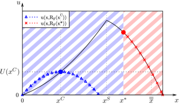
Figure 1: Duopoly example with a simple CST

We set for now $d=0$ and $r=4/5$. Figure 1 depicts the corresponding $U$. The (unique) Cournot and Stackelberg actions are, respectively, $x^{C}=5/11$ and $x^{S}=1$. The quantity $\overline{\overline{x}}$ solves $U(\overline{\overline{x}})=U(x^{C})$. The curve in blue (respectively, red) gives the payoffs of the leader given that the follower best-responds to $x^{C}$ (respectively, $x^{*}=3/2$).

A simple commitment structure.

We first examine the simple commitment structure

$$\left\{\left[0,\frac{3}{2}\right),\left[\frac{3}{2},\frac{5}{3}\right]\right\}.$$

This CST might describe a situation in which the leader can invest in new equipment to increase its productive capacity. Without the new equipment, the leader produces less than $3/2$; following the investment, the leader produces at least $3/2$.

Any quantity in the interval $[3/2,5/3]$ is such that, whenever the follower best-responds, the leader benefits from deviating to a smaller quantity. Hence, any subgame perfect equilibrium must be such that the leader produces $3/2$ in the corresponding subgame. If instead the leader picks $[0,3/2)$ in the first period, then each firm produces the Cournot quantity. As $U(3/2)>U(x^{C})$, the unique subgame perfect equilibrium is such that the leader commits to the upper interval.

The previous reasoning applies if $3/2$ is replaced by any quantity $x^{*}$ in the interval $[x^{C},\bar{\bar{x}}]$. Consequently, all actions in $[x^{C},\bar{\bar{x}}]$ are simply plausible. A corollary of Theorem 1 is that these actions constitute the entire set of simply-plausible actions.

A commitment structure that violates Property I.

We now consider the commitment structure

$$\left\{\left(\frac{1}{8},\frac{1}{3}\right],\left[0,\frac{1}{8}\right]\cup\left(\frac{1}{3},\frac{5}{3}\right]\right\}.$$

This CST might represent a situation in which the leader faces three options: rely on old equipment and produce at most $1/8$, get new equipment and produce some quantity in $(1/8,1/3]$, or outsource production to produce more than $1/3$. Figure 2 illustrates this example. The curve in red (respectively, blue) gives the payoffs of the leader given that the follower best-responds to $1/3$ (respectively, $1/8$).

Figure 2: Duopoly example with a CST that violates Property I

The subgame following the choice of $(1/8,1/3]$ has a unique equilibrium, in which the leader produces $1/3$. The other subgame has two equilibria: one yielding the Cournot outcome, the other involving the leader choosing quantity $1/8$. Hence, there are two subgame perfect equilibria. In one of them the leader produces $1/3$, while in the other the leader produces $x^{C}$. In the former equilibrium, the leader anticipates that if she were to select $\left[0,1/8\right]\cup\left(1/3,5/3\right]$ in the first period, the follower would respond by producing a quantity larger than $x^{C}$. Consequently, the leader settles for the quantity $1/3$, thus obtaining a payoff smaller than $U(x^{C})$. We show in Section 6 that this example illustrates a more general point: beyond simple CSTs, the Cournot payoffs generally do not bound from below the payoffs that the leader can obtain.

3.2 A Coordination Game

The Setting.

In this subsection, we examine the following coordination game. The action spaces are $\mathcal{X}=\mathcal{Y}=[0,1]$. The payoffs of the leader are given by

$$u(x,y)=xy+(1-x)(1-y)-\frac{1}{2}\left(x-\frac{1}{2}\right)^{2}-\frac{3(1+a)}{2}\left(y-\frac{1}{2}\right)^{2},$$

for some $a\geq 0$. The payoffs of the follower are given $v(y,x)=u(y,x)$. This setting might capture a situation in which two firms with complementary production processes choose the locations of their plants. The first two terms of the function $u$ capture the firms’ desire to be close to each other. The remaining terms capture intrinsic features specific to the different locations.

We set for now $a=0$. Figure 3 depicts the corresponding $U$. The leader’s Stackelberg actions are $0$, $1/2$ and $1$; in fact, these are also the leader’s Cournot actions (henceforth represented by the generic notation $x^{C}_{n}$). The curve in red (respectively, blue) gives the payoffs of the leader given that the follower best-responds to $x^{*}$ (respectively, $1-x^{*}$).

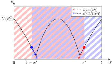
Figure 3: Coordination game example with a CST that violates property P

A commitment structure that violates Property P.

Fix $x^{*}\in(1/2,1)$ and consider the commitment structure

$$\big{\{}[0,x^{*}],[1-x^{*},1]\big{\}}.$$

This CST might represent a situation in which the leader can commit either not to locate near $1$, or not to locate near $0$. Notice that this commitment structure does not partition the leader’s action space: actions in $[1-x^{*},x^{*}]$ belong to both elements of the CST.

The subgame induced by the leader’s choice of $[0,x^{*}]$ has an equilibrium in which the leader locates at $x^{*}$. Symmetrically, following the first-period choice of $[1-x^{*},1]$, an equilibrium exists in which the leader locates at $1-x^{*}$. Since $U(x^{*})=U(1-x^{*})$, in one subgame perfect equilibrium the leader locates at $x^{*}$, while in another the leader locates at $1-x^{*}$. As $x^{*}$ could take any value in $(1/2,1)$, we see that all actions are in fact plausible. In sharp contrast, a corollary of Theorem 1 shows that the only simply-plausible actions are $0$, $1/2$, and $1$.

4 Preliminaries

Let

$$\eta(\tilde{x},x):=u\big{(}\tilde{x},R_{F}(x)\big{)}-u\big{(}x,R_{F}(x)\big{)}.$$

In words, $\eta(\tilde{x},x)$ measures the leader’s gain from choosing $\tilde{x}$ instead of $x$ when the follower best-responds to $x$. Now consider an arbitrary commitment structure $K$. Suppose that a subgame perfect equilibrium of $G(K)$ exists. Given $\mathcal{X}_{i}\in K$, write $\beta(\mathcal{X}_{i})$ for the leader’s action in the subgame following $\mathcal{X}_{i}$. Then $\beta(\mathcal{X}_{i})\in\mathcal{X}_{i}$, and $\eta\big{(}x,\beta(\mathcal{X}_{i})\big{)}\leq 0$ for all $x\in\mathcal{X}_{i}$. The notion of admissible pair summarizes these basic properties.

Definition 4.1.

A pair $(K,\beta)$ made up of a commitment structure $K$ and a mapping $\beta:K\rightarrow\mathcal{X}$ is said to be admissible if

1. $\beta(\mathcal{X}_{i})\in\mathcal{X}_{i}$, for all $\mathcal{X}_{i}\in K;$

2. $\eta\big{(}x,\beta(\mathcal{X}_{i})\big{)}\leq 0$, for all $\mathcal{X}_{i}\in K$ and all $x\in\mathcal{X}_{i}$.

By construction, each admissible pair $(K,\beta)$ is associated with at least one subgame perfect equilibrium of $G(K)$, and vice versa. We next formalize this basic observation for future reference.

Lemma 4.1.

An outcome $(x,y)$ is plausible if and only if there exist an admissible pair $(K,\beta)$ and $\mathcal{X}_{i}\in K$, such that

1. $x=\beta(\mathcal{X}_{i})$,

2. $U\big{(}\beta(\mathcal{X}_{i})\big{)}=\max_{\mathcal{X}_{j}\in K}U\big{(}\beta(\mathcal{X}_{j})\big{)}$,

3. $y=R_{F}(x)$.

• Let $(x,y)$ be plausible, and $K$ a CST such that $(x,y)$ is the outcome of the subgame perfect equilibrium $\mathcal{E}$ of $G(K)$. Let $\mathcal{X}_{i}\in K$ denote the first-period choice of the leader in equilibrium $\mathcal{E}$. Furthermore, for every $\mathcal{X}_{j}\in K$, let $\beta(\mathcal{X}_{j})$ denote the action of the leader in the subgame induced by the choice of subset $\mathcal{X}_{j}$. Then, by definition of subgame perfect equilibrium, $(K,\beta)$ is an admissible pair that satisfies (i)-(iii). The converse is immediate. $\blacksquare$

Any pair $(K,\beta)$ satisfying the conditions of the lemma will be said to implement outcome $(x,y)$.

5 Simple Commitment Structures

This section contains the first part of our core analysis. We characterize the set of simply-plausible outcomes and show that the Stackelberg and Cournot payoffs bound the payoffs attainable by the leader under any simple CST. All proofs not in the main text are in Appendix A.

Denote by $R_{L}(y)$ the unique best response of the leader to the follower’s action $y$, and define

$$\phi(x):=R_{L}\big{(}R_{F}(x)\big{)}.$$

Thus, in particular, the fixed points of $\phi$ are the Cournot actions of the leader. For brevity, in what follows let $\mathcal{X}^{C}$ denote said set of Cournot actions; the notation $x^{C}_{n}$ will indicate a generic element of this set.

Lemma 5.1.

Let $K$ be a simple commitment structure. Then $(K,\beta)$ is admissible if and only if, for all $\mathcal{X}_{i}\in K$, one of the following conditions holds:

1. $\beta(\mathcal{X}_{i})\in\mathcal{X}_{i}\cap\mathcal{X}^{C}$;

2. $\beta(\mathcal{X}_{i})=\min\mathcal{X}_{i}$ and $\phi\big{(}\beta(\mathcal{X}_{i})\big{)}<\beta(\mathcal{X}_{i})$;

3. $\beta(\mathcal{X}_{i})=\max\mathcal{X}_{i}$ and $\phi\big{(}\beta(\mathcal{X}_{i})\big{)}>\beta(\mathcal{X}_{i})$.

Figure 4, panel A, illustrates the result in the context of the duopoly example, for parameter values $d=0$ and $r=6/5$. The black curve represents the graph of the function $\phi$. The leader’s Cournot actions are $x_{1}^{C}=0$, $x_{2}^{C}=5/9$, and $x_{3}^{C}=5/4$. An admissible pair $(K,\beta)$ must be such that every action $\beta(\mathcal{X}_{i})$ which belongs to a region of the figure comprising a left-pointing arrow (respectively, right-pointing arrow) is either a Cournot action or the leftmost (respectively, rightmost) element of $\mathcal{X}_{i}$.

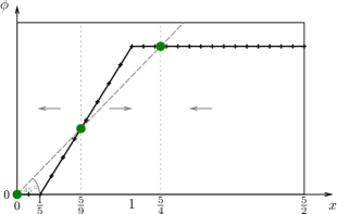
(a)

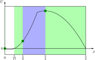
(b)

Figure 4: Duopoly Example, for $d=0$ and $r=6/5$

Our first theorem characterizes the set of simply-plausible outcomes.

Theorem 1.

An action $x^{*}$ is simply plausible if and only if the lower contour set of $x^{*}$ with respect to $U$ contains a Cournot action $x_{n^{*}}^{C}$ such that

$$\big{(}\phi(x^{*})-x^{*}\big{)}\big{(}x_{n^{*}}^{C}-x^{*}\big{)}\geq 0.$$ (2)

The proof of the if part of the theorem is easy. Consider $x^{*}$ such that $\phi(x^{*})>x^{*}$. Let (2) hold for some $x_{n^{*}}^{C}$ such that $U(x_{n^{*}}^{C})\leq U(x^{*})$. Now consider $K=\big{\{}[\underline{x},x^{*}],(x^{*},\overline{x}]\big{\}}$, and $\beta$ given by $\beta\big{(}[\underline{x},x^{*}]\big{)}=x^{*}$ and $\beta\big{(}(x^{*},\overline{x}]\big{)}=x_{n^{*}}^{C}$. The pair $(K,\beta)$ is admissible and implements $x^{*}$. The proof of the only if part of the theorem is in the appendix.

Applying Theorem 1 to the example of Figure 4 shows that the set of simply-plausible actions is equal to $\{0\}\cup\big{[}5/17,5/9\big{]}\cup\big{[}5/4,5/2\big{]}$. Firstly, Theorem 1 shows that no action in the interval $\big{(}0,5/17\big{)}$ is simply plausible, since all of them belong to the strict lower contour set of each Cournot action (see panel B). Secondly, any $x\in\big{(}5/9,5/4\big{)}$ satisfies $\phi(x)>x$ (see panel A). The only Cournot action greater than any of these actions is $x_{3}^{C}$. As $U(x_{3}^{C})>U(x)$ for all $x\in\big{(}5/9,5/4\big{)}$, we conclude using Theorem 1 that no action in this interval is simply plausible. Mirror arguments show that all actions in $\{0\}\cup\big{[}5/17,5/9\big{]}\cup\big{[}5/4,5/2\big{]}$ are simply plausible.

By construction, the leader’s Stackelberg payoff provides an upper bound for the payoffs attainable by the leader under any CST. Theorem 1 shows that the Cournot payoffs provide a corresponding lower bound for simple CSTs. The theorem also tells us that if an action is in the upper contour set of all Cournot actions, then that action must be simply plausible. The following corollary records these observations.

Corollary 5.1.

All simply-plausible actions belong to the upper contour set of a Cournot action with respect to $U$. Any action in the intersection of these upper contour sets is simply plausible.

We will see in the next section that the first part of the corollary ceases to be true beyond simple CSTs. On the other hand, relaxing the constraints imposed on simple CSTs (i.e., Property P and Property I) ensures the plausibility of any action belonging to the upper contour set of some Cournot action. By contrast, the example of Figure 4 shows that an action may belong to the upper contour set of a Cournot action and fail to be simply plausible.

6 General Commitment Structures

In this section, we expand the class of commitment structures considered. Recall that a commitment structure is simple if it is an interval partition of the leader’s action space. We first relax (in Subsection 6.1) the requirement that the commitment structure is a partition of the leader’s action space. We then study (in Subsection 6.2) commitment structures comprising non-convex sets.

6.1 I-Plausibility

We say that an outcome $(x,y)$ is I-plausible if it is a subgame perfect equilibrium outcome of $G(K)$ for some commitment structure $K$ comprising only intervals. Thus, every simply-plausible outcome is also I-plausible, but an outcome may be I-plausible without being simply plausible. Our next theorem characterizes the set of I-plausible outcomes. All proofs for this subsection are in Appendix B.

Theorem 2.

An action $x^{*}$ is I-plausible if and only if the lower contour set of $x^{*}$ with respect to $U$ includes actions $x^{\prime}$ and $x^{\prime\prime}$ such that

$$\phi(x^{\prime})\leq x^{\prime}\leq x^{\prime\prime}\leq\phi(x^{\prime\prime}).$$ (3)

The proof of the if part of the theorem is straightforward. Let $x^{*}$ be such that the lower contour set of $x^{*}$ with respect to $U$ includes actions $x^{\prime}$ and $x^{\prime\prime}$ satisfying (3). Consider $K=\big{\{}\{x^{*}\},[\underline{x},x^{\prime\prime}],[x^{\prime},\overline{x}]\big{\}}$, and $\beta$ given by $\beta\big{(}\{x^{*}\}\big{)}=x^{*}$, $\beta\big{(}[\underline{x},x^{\prime\prime}]\big{)}=x^{\prime\prime}$, and $\beta\big{(}[x^{\prime},\overline{x}]\big{)}=x^{\prime}$. The pair $(K,\beta)$ is admissible and implements $x^{*}$. The proof of the only if part of the theorem is in the appendix.

The following corollary of Theorem 2 is immediate.

Corollary 6.1.

All actions in the upper contour set of a Cournot action with respect to $U$ are I-plausible.

Using Theorem 2 in the example of Figure 4 shows that the set of I-plausible actions is equal to $\{0\}\cup\big{[}5/17,5/2\big{]}$. Indeed, by Corollary 6.1, all actions in $\{0\}\cup\big{[}5/17,5/2\big{]}$ are I-plausible. Moreover, any $x^{*}\in\big{(}0,5/17\big{)}$ is such that the intersection between $\{x:\phi(x)\geq x\}$ and the lower contour set of $x^{*}$ with respect to $U$ is empty. By applying Theorem 2, we conclude that no action in $\big{(}0,5/17\big{)}$ is I-plausible.

Example 3 (Subsection 3.2) shows that Corollary 5.1 from Section 5 ceases to be true for I-plausible outcomes: an outcome may be I-plausible and give the leader a smaller payoff that any of the Cournot outcomes. The propositions which follow provide sufficient conditions under which the conclusion of Corollary 5.1 can be extended.

Proposition 6.1.

Suppose $U$ is either quasi-convex or quasi-concave. Then, an action is I-plausible if and only if it belongs to the union of the upper contour sets of the Cournot actions with respect to $U$.

Proposition 6.2.

If there exists a unique Cournot outcome, then the set of I-plausible actions coincides with the set of simply-plausible ones. In this case, both sets are equal to the upper contour set of the unique Cournot action with respect to $U$.

6.2 P-Plausibility

We say that an outcome $(x,y)$ is P-plausible if it is a subgame perfect equilibrium outcome of $G(K)$ for some commitment structure $K$ partitioning the leader’s action space. Thus, every simply-plausible outcome is also P-plausible, but an outcome may be P-plausible without being simply plausible. Commitment structures that partition the leader’s action space can take complicated forms. To keep the analysis tractable, we characterize here the set of P-plausible outcomes in settings that satisfy three regularity conditions:

1. $\mathcal{X}^{C}=\big{\{}x^{C}\big{\}}$, with $x^{C}\in\text{int}({\mathcal{X}})$ and $y^{C}:=R_{F}(x^{C})\in\text{int}({\mathcal{Y}})$;

2. $\leavevmode\nobreak\ u_{2}v_{2}>0$;

3. $\leavevmode\nobreak\ u_{12}v_{12}>0$.

Condition (RC1) supposes the existence of a unique Cournot outcome. Condition (RC2) ensures homogeneous payoff externalities: these could be positive or negative, but cannot change sign. Similarly, condition (RC3) ensures homogeneous strategic interactions: actions may be strategic complements or substitutes, but cannot be both.

For every $x\in\mathcal{X}$, the function $\eta(\cdot,x)$ is strictly concave and satisfies $\eta(x,x)=0$. It follows that $\eta(\tilde{x},x)=0$ for at most one action $\tilde{x}$ different from $x$. We can thus define $\gamma:\mathcal{X}\rightarrow\mathcal{X}$ as follows: if $\eta(\tilde{x},x)=0$ for some $\tilde{x}\neq x$, set $\gamma(x)=\tilde{x}$; otherwise, set

$$\gamma(x)=\begin{cases}\overline{x}&\text{if $x<x^{C}$},\\ x^{C}&\text{if $x=x^{C}$},\\ \underline{x}&\text{if $x>x^{C}$}.\\ \end{cases}$$

The interpretation is straightforward: in cases where such an action exists, $\gamma(x)$ is the action making the leader indifferent between choosing $x$ or $\gamma(x)$ when the follower best-responds to $x$.

Next, let

$$\mathcal{S}:=\begin{cases}\big{\{}x:\;x\leq\gamma(x)\leq x^{C}\big{\}}&\text{if $u_{2}u_{12}>0$},\\ \big{\{}x:\;x^{C}\leq\gamma(x)\leq x\big{\}}&\text{if $u_{2}u_{12}<0$}.\end{cases}$$

Note that, as $\gamma$ is continuous, the set $\mathcal{S}$ is compact. Moreover, this set evidently contains $x^{C}$. We are now ready to characterize the P-plausible outcomes. All proofs for this subsection are in Appendix C.

Theorem 3.

Suppose (RC1)–(RC3) hold. The set of P-plausible actions coincides with the upper level set of $\underline{U}:=\min_{x\in\mathcal{S}}\;U\big{(}\gamma(x)\big{)}$ with respect to $U$.

We illustrate here the previous theorem in the context of the duopoly example with parameter values $d=0$ and $r=4/5$. In Figure 5, panel A, the black curve represents the graph of the function $\phi$, which crosses the 45-degree line at $x^{C}=5/11$. In this example, $\mathcal{S}=\big{\{}x:\;x\leq\gamma(x)\leq x^{C}\big{\}}$. The gray curve represents the graph of $\gamma$: we see that $\mathcal{S}=[0,x^{C}]$ and $\gamma(\mathcal{S})=\big{[}5/18,x^{C}\big{]}$. Panel B depicts the graph of the function $U$. Minimizing $U$ over $\gamma(\mathcal{S})$ shows that $\underline{U}=U\big{(}5/18\big{)}$. The upper level set of $\underline{U}$ corresponds to $\big{[}5/18,\hat{x}_{2}\big{]}$. Since the upper contour set of $x^{C}$ with respect to $U$ is equal to $\big{[}x^{C},\hat{x}_{1}\big{]}$, coupling Theorem 3 with Proposition 6.2 shows that the P-plausible outcomes form a strict superset of the simply-plausible ones.

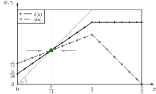
(a)

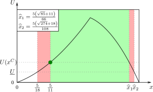
(b)

Figure 5: Duopoly Example, for $d=0$ and $r=4/5$

We next illustrate the basic idea underlying Theorem 3 in the context of the previous example. We will argue that $1/3$ is P-plausible, even though that action is not simply plausible. Let $\mathcal{X}_{1}:=\left\{0\right\}\cup\big{(}1/3,5/3\big{]}$, $\mathcal{X}_{2}:=\big{(}0,1/3\big{]}$, and consider the pair $(K,\beta)$ where $K=\{\mathcal{X}_{1},\mathcal{X}_{2}\}$, $\beta(\mathcal{X}_{1})=0$, and $\beta(\mathcal{X}_{2})=1/3$. It is easy to verify that $\eta\big{(}x,1/3\big{)}<0$ for all $x<1/3$. Next, as $\phi(0)>0$ the definition of $\gamma$ yields $\eta(x,0)<0$ for every $x>\gamma(0)$. Since $\gamma(0)<1/3$ (see panel A), we thus obtain $\eta(x,0)<0$ for all $x\in\big{(}1/3,5/3\big{]}$. Combining the previous observations shows that $(K,\beta)$ constitutes an admissible pair. Moreover, as $U(1/3)>U(0)$, we see that $(K,\beta)$ implements $1/3$.

In the previous example, $\underline{U}$ is less than the leader’s Cournot payoff. The question remains as to whether we can find conditions that guarantee $\underline{U}<U(x^{C})$. We show in Appendix C that a simple sufficient condition is given by $\gamma^{\prime}(x^{C})>0$. Calculations relegated to Appendix C establish that $\gamma^{\prime}(x^{C})>0$ if and only if $R_{L}^{\prime}(y^{C})R_{F}^{\prime}(x^{C})>1/2$. We thus obtain:

Proposition 6.3.

Suppose (RC1)–(RC3) hold. If $R_{L}^{\prime}(y^{C})R_{F}^{\prime}(x^{C})>1/2$ then $\underline{U}<U(x^{C})$.

7 Commitment Design

In this section, we apply our results to study the problem of a designer choosing a commitment structure so as to achieve some objective. All proofs for this section are in Online Appendix OA.

Let $\mathcal{K}$ be some arbitrary class of commitment structures. As usual, say that an outcome $(x,y)$ is $\mathcal{K}$-plausible if $(x,y)$ is a subgame perfect equilibrium outcome of $G(K)$, for some commitment structure $K\in\mathcal{K}$. We write $\underline{x}^{\mathcal{K}}$ (respectively, $\overline{x}^{\mathcal{K}}$) for the smallest (respectively, largest) $\mathcal{K}$-plausible action of the leader.

The general commitment design problem takes the following form:

$$\max W(x,R_{F}(x))\leavevmode\nobreak\ \leavevmode\nobreak\ x \mathcal{K}$$ s.t. is -plausible, (CDP)

for some objective function $W(x,y)$.

In the remainder, we explore various commitment design problems in the context of the duopoly example presented in Subsection 3.1. We first examine situations where the designer is one of the two firms. The Stackelberg outcome is plainly the best plausible outcome from the perspective of the leader. On the other hand, since $v_{2}$ is here negative, the optimal plausible outcome from the perspective of the follower involves the leader producing as little as plausibly possible. The proposition which follows summarizes these observations.

Proposition 7.1.

Suppose $\mathcal{K}$ is the set of all commitment structures. Then:

1. for $W=u$, the unique solution of (CDP) is $x^{S}$;

2. for $W=v$, the unique solution of (CDP) is $\underline{x}^{\mathcal{K}}$.

The Stackelberg CST is optimal for the leader. The Cournot CST is optimal for the follower if and only if $r\notin\big{(}r^{*}(d),d+1\big{)}$, where $r^{*}(d):=2-\sqrt{2}(1-d)$. For $r\in\big{(}r^{*}(d),d+1\big{)}$, the CST

$$\Big{\{}\big{(}0,\gamma(0)\big{]},\{0\}\cup\big{(}\gamma(0),\overline{x}\big{]}\Big{\}}$$

is optimal for the follower. The latter CST is such that the leader either commits to producing a quantity in the interval $\big{(}0,\gamma(0)\big{]}$, or commits to producing a quantity outside of this interval.

We next examine situations in which the designer aims to maximize either consumer surplus, producer surplus, or total welfare (i.e., the sum of producer and consumer surplus). We follow Singh and Vives (1984) and define the consumer surplus generated by an outcome $(x,y)$ as

$$CS(x,y)=\frac{(x+y)^{2}}{2}-dxy.$$

Producer surplus is defined as

$$PS(x,y)=u(x,y)+v(y,x).$$

Proposition 7.2.

Suppose $\mathcal{K}$ is the set of all commitment structures. Then:

1. for $W=CS$, the unique solution of (CDP) is $\overline{x}^{\mathcal{K}}$;

2. for $W=PS$, the unique solution of (CDP) is $x^{C}$ if $r<r^{\dagger}(d)$, and $x^{S}$ if $r^{\dagger}(d)<r<d+1$; if $r>d+1$ then the solutions are $x_{3}^{C}$ and $0$;

3. for $W=CS+PS$, the unique solution of (CDP) is $\overline{x}^{\mathcal{K}}$.

Part (i) of Proposition 7.2 is explained as follows. Firstly, we show that consumer surplus is a convex function of the quantity which the leader produces. The problem of the designer therefore reduces to choosing between $\underline{x}^{\mathcal{K}}$ and $\overline{x}^{\mathcal{K}}$. Inducing the leader to produce $\overline{x}^{\mathcal{K}}$ instead of $\underline{x}^{\mathcal{K}}$ is optimal because in this way the designer can exploit the strategic motive to produce large quantities which arises from commitment. With multiple Cournot actions, or if there exists a single Cournot action and $\gamma(0)\geq x^{C}$, the binary partition $\big{\{}[\underline{x},\overline{x}^{\mathcal{K}}),[\overline{x}^{\mathcal{K}},\overline{x}]\big{\}}$ is consumer-optimal. Otherwise, the CST

$$\Big{\{}\big{(}0,\gamma(0)\big{]},\{0\}\cup\big{(}\gamma(0),\overline{x}^{\mathcal{K}}\big{)},\big{[}\overline{x}^{\mathcal{K}},\overline{x}\big{]}\Big{\}}$$

is optimal for the consumer. The latter CST is such that the leader either commits to producing a quantity in the interval $\big{(}0,\gamma(0)\big{]}$, or commits to producing a quantity outside of this interval; in the latter case, the leader either commits to producing a quantity at least as large as $\overline{x}^{\mathcal{K}}$, or commits to producing less than this.

Part (ii) of Proposition 7.2 is straightforward. With decreasing returns to scale, producer surplus is maximized by inducing both firms to produce the same quantity; in this case, the Cournot CST is producer-optimal. By contrast, with large returns to scale, producer surplus is maximized by letting one firm acquire a bigger market share than the other. In particular, for very large returns to scale, producer surplus is maximized by letting one firm act as a monopolist. Consequently, the Cournot CST is producer-optimal for extreme returns to scale, whereas the Stackelberg CST is producer-optimal for sufficiently large returns to scale.

Part (iii) of Proposition 7.2 follows from the fact that producer surplus tends to be less sensitive than consumer surplus to the quantity which the leader produces. So maximizing total welfare implies maximizing consumer surplus.

8 Discussion

8.1 Refinements

Our results show that the Stackelberg and Cournot payoffs provide the bounds of the payoffs attainable by the leader under any simple CST. A natural question is whether some equilibrium refinement ensures that the Stackelberg and Cournot payoffs provide the bounds of the payoffs attainable by the leader under arbitrary CSTs.

Forward induction type of arguments eliminate some, but not all, subgame perfect equilibria giving the leader less than her Cournot payoffs. For instance, consider the setting of Example 3 in Subsection 3.2, but this time with commitment structure

$$\left\{\left[\frac{1}{9},\frac{4}{9}\right),\left[0,\frac{1}{9}\right)\cup\left[\frac{4}{9},1\right)\right\}.$$

Figure 6 depicts the graph of $U$. The curve in red (respectively, blue) gives the payoffs of the leader given that the follower best-responds to $1/9$ (respectively, $4/9$). The subgame induced by the leader’s choice of $[1/9,4/9)$ has a unique equilibrium, in which the leader locates at $1/9$. The other subgame has an equilibrium in which the leader picks $4/9$. As $U(4/9)>U(1/9)$, a subgame perfect equilibrium exists in which the leader chooses $4/9$. Yet, $U(4/9)<U(x^{C}_{n})$, so the leader obtains a payoff smaller than her Cournot payoff. Since the subgame off the equilibrium path possesses a unique equilibrium, forward induction type of arguments have no bite.

Figure 6: Coordination game example, with a CST that violates Property I

One alternative is to restrict attention to subgame perfect equilibria that select, in every period-2 subgame, the best continuation equilibrium from the perspective of the leader. In this case, any subgame induced by the leader’s period-1 choice of a subset containing a Cournot action must give the leader a payoff at least as large as the corresponding Cournot payoff. Consequently, any such subgame perfect equilibrium ensures that the leader obtains at least her maximum Cournot payoff.

8.2 Richer vs Finer Commitment

We explore here the intuitive notion that two commitment structures might give different “degrees” of commitment to the leader. Two natural partial orders on the set of commitment structures emerge from our analysis. Firstly, we say that a CST $K^{\prime}$ is richer than a CST $K$ if $K\subseteq K^{\prime}$. Secondly, we say that a CST $K^{\prime}$ is finer than a CST $K$ if the following conditions hold:

1. each element $\mathcal{X}^{\prime}_{i}$ of the CST $K^{\prime}$ is a subset of some element $\mathcal{X}_{i}$ of the CST $K$,

2. each element of $K$ can be written as the union of elements of $K^{\prime}$.

In other words, $K^{\prime}$ is finer than $K$ if $K^{\prime}$ can be obtained from $K$ by replacing each element $\mathcal{X}_{i}$ of $K$ by some cover of $\mathcal{X}_{i}$.

Finally, given a CST $K$ such that the set of subgame perfect equilibria of $G(K)$ is non-empty, say that a CST $K^{\prime}$ is worse than $K$ if some subgame perfect equilibrium of $G(K^{\prime})$ gives the leader a strictly lower payoff than every subgame perfect equilibrium of $G(K)$.

It is not hard to see that, starting from a given CST, either enriching this CST or refining it can make the leader better off. It is equally clear that a CST cannot be both richer and worse than another one. By contrast, our analysis reveals that a CST may be finer and worse than another CST. Indeed, every CST is finer than the Cournot CST. A corollary of our analysis is thus that refining the Cournot CST can yield a CST that is worse.

A second corollary of our analysis is that every CST that refines the Cournot CST and is worse than it must be non-simple. A natural question is therefore whether, by restricting attention to simple CSTs, we ensure that a CST that is finer than another one is not also worse. The following example shows that the answer is no.

Consider the coordination game from Subsection 3.2, where $a$ takes a small positive value. This setting has three Cournot actions ($0$, $1/2$, and $1$) but only one Stackelberg action ($1/2$). Now consider the simple CST

$$K=\big{\{}\{0\},(0,1),\{1\}\big{\}}.$$

Let $\nu$ be a small positive number, and denote by $K^{\prime}$ the CST comprising $[\nu,1-\nu]$ and all singletons $\{x\}$ where $x\in\mathcal{X}\setminus[\nu,1-\nu]$. Notice that $K^{\prime}$ is a finer partition than $K$. The game $G(K)$ has a unique subgame perfect equilibrium outcome: $(1/2,1/2)$. However, the game $G(K^{\prime})$ has three subgame perfect equilibrium outcomes, namely, $(1/2,1/2)$, $(0,0)$, and $(1,1)$. As $U(0)<U(1/2)$, and $U(1)<U(1/2)$, $K^{\prime}$ is worse than $K$. We show in the Online Appendix that Theorems 1 and 2 yield a method for checking whether a CST can be refined by some worse CST.

8.3 Quasi-Simple Commitment Structures

Our analysis shows that the set of plausible outcomes is typically larger than the set of simply-plausible ones. A natural question is whether a subset of relatively basic CSTs generates the entire set of plausible outcomes. Our next result shows that in somewhat well-behaved environments (those satisfying (RC1)–(RC3)), the answer is yes.

We say that an outcome is quasi-simply plausible if it is a subgame perfect equilibrium outcome of $G(K)$ for some commitment structure $K$ that partitions the leader’s action space and contains at most one element that is not an interval.

Proposition 8.1.

Suppose (RC1)–(RC3) hold. Then every plausible outcome is quasi-simply plausible.

The proof is in the online appendix. In fact, it can be shown that if $U$ is either quasi-concave or quasi-convex then all plausible outcomes can be implemented with a partition of the leader’s action space such that each partition element is either an interval or a union of two intervals. Effectively, these commitment structures are such that the leader plainly commits to choosing an action: (a) inside or outside an interval, (b) below or above a cutoff.

9 Conclusion

The Stackelberg leadership model assumes that the leader can commit to any action she might choose. Our paper takes a different view: we only assume that the leader can commit not to take certain subsets of actions.

We provide a tractable model of commitment that encompasses the Stackelberg and Cournot models as special cases but also enables us to capture situations of partial commitment. We characterize the set of outcomes resulting from all possible commitment structures, and shed light thereby on the “limits of commitment”. Our results highlight that, more than commitment, what matters is the precise form that commitment takes. For instance, we show that whereas the Stackelberg and Cournot payoffs provide the bounds of the payoffs attainable by the leader under some appropriately defined class of “simple” commitment structures, this property fails to hold more generally.

Appendix A Appendix of Section 5

Throughout the appendix, the lower contour set of $x$ with respect to $U$ will be denoted by $\mathcal{Q}_{\leq}(x)$, that is,

$$\mathcal{Q}_{\geq}(x):=\big{\{}\tilde{x}:\leavevmode\nobreak\ U(\tilde{x})\geq U(x)\big{\}}.$$

The sets $\mathcal{Q}_{<}(x)$, $\mathcal{Q}_{\geq}(x)$, and $\mathcal{Q}_{>}(x)$ are similarly defined. When we deem the chances of confusion sufficiently small, we will talk about, e.g., the upper contour set of $x$, without explicit reference to $U$.

• We prove the only if part of the lemma; the proof of the other part is similar. Suppose that $(K,\beta)$ constitutes an admissible pair. Reason by contradiction, and suppose that we can find $\mathcal{X}_{i}\in K$ such that $\phi\big{(}\beta(\mathcal{X}_{i})\big{)}<\beta(\mathcal{X}_{i})$ while $\beta(\mathcal{X}_{i})\neq\min\mathcal{X}_{i}$. The function $\eta\big{(}\cdot,\beta(\mathcal{X}_{i})\big{)}$ is strictly concave, maximized at $\phi\big{(}\beta(\mathcal{X}_{i})\big{)}$, and satisfies $\eta\big{(}\beta(\mathcal{X}_{i}),\beta(\mathcal{X}_{i})\big{)}=0$. So $\eta\big{(}x,\beta(\mathcal{X}_{i})\big{)}>0$ for all $x\in\big{[}\phi\big{(}\beta(\mathcal{X}_{i})\big{)},\beta(\mathcal{X}_{i})\big{)}$. Since $\mathcal{X}_{i}$ is an interval, $\beta(\mathcal{X}_{i})\in\mathcal{X}_{i}$, and $\beta(\mathcal{X}_{i})\neq\min\mathcal{X}_{i}$, we can find $\varepsilon>0$ such that $\big{(}\beta(\mathcal{X}_{i})-\varepsilon,\beta(\mathcal{X}_{i})\big{)}\subset\mathcal{X}_{i}$. Coupling the previous remarks shows the existence of $x\in\mathcal{X}_{i}$ such that $\eta\big{(}x,\beta(\mathcal{X}_{i})\big{)}>0$; this contradicts the assumption that $(K,\beta)$ is admissible. Hence, $\phi\big{(}\beta(\mathcal{X}_{i})\big{)}<\beta(\mathcal{X}_{i})$ implies $\beta(\mathcal{X}_{i})=\min\mathcal{X}_{i}$. Analogous arguments show that $\phi\big{(}\beta(\mathcal{X}_{i})\big{)}>\beta(\mathcal{X}_{i})$ implies $\beta(\mathcal{X}_{i})=\max\mathcal{X}_{i}$. $\blacksquare$

• The if part of the theorem was proven in the text; we prove here the converse. Pick an arbitrary simply-plausible action $x^{*}$. We aim to prove the existence of a Cournot action $x_{n^{*}}^{C}\in\mathcal{Q}_{\leq}(x^{*})$ such that (2) holds. If $\phi(x^{*})=x^{*}$, just take $x_{n^{*}}^{C}=x^{*}$; we treat below the case in which $\phi(x^{*})>x^{*}$ (the remaining case is analogous). Reason by contradiction, and suppose that

  $$\mathcal{X}^{C}\cap(x^{*},\overline{x}]\cap\mathcal{Q}_{\leq}(x^{*})=\varnothing.$$ (4)

  Let $(K,\beta)$ implement $x^{*}$, with $K$ simply plausible . We will show that $K$ cannot be finite. By Berge’s maximum theorem, both $R_{F}$ and $R_{L}$ are continuous, thus $\phi$ is continuous as well. As $\phi(x^{*})>x^{*}$ and $\phi(\overline{x})\leq\overline{x}$, the intermediate value theorem shows that

  $$\mathcal{X}^{C}\cap(x^{*},\overline{x}]\neq\varnothing.$$

  Note that the continuity of the function $\phi$ implies the compactness of $\mathcal{X}^{C}$. So $\mathcal{X}^{C}\cap(x^{*},\overline{x}]=\mathcal{X}^{C}\cap[x^{*},\overline{x}]$ possesses a smallest element, that we denote by $x_{1}^{C}$. Let $\mathcal{X}_{1}$ be the member of $K$ containing $x_{1}^{C}$. Then Lemma 5.1 combined with (4) gives

  $$\beta(\mathcal{X}_{1})\in(x_{1}^{C},\overline{x}]\cap\big{\{}x:\phi(x)>x\big{\}}.$$

  Now let $x_{2}^{C}$ be the smallest Cournot action greater than $\beta(\mathcal{X}_{1})$, and denote by $\mathcal{X}_{2}$ the member of $K$ containing $x_{2}^{C}$. The same logic as above gives $\beta(\mathcal{X}_{2})\in(x_{2}^{C},\overline{x}]\cap\big{\{}x:\phi(x)>x\big{\}}$, and so on. If $K$ were finite, the previous iteration would have to end after finitely many steps, say $m$. But then $\beta(\mathcal{X}_{m})=\overline{x}$ and $\beta(\mathcal{X}_{m})\in\big{\{}x:\phi(x)>x\big{\}}$, giving $\phi(\overline{x})>\overline{x}$. The previous contradiction proves that $K$ cannot be finite.

We proceed to show that $K$ cannot be infinite either. The function $U$ is continuous and, by (4), $U(x_{n}^{C})>U(x^{*})$ for all $x_{n}^{C}\in\mathcal{X}^{C}\cap(x^{*},\overline{x}]$. Furthermore, as already pointed out above, $\mathcal{X}^{C}\cap(x^{*},\overline{x}]$ is a compact set. Therefore,

$$\Delta:=\min_{x_{n}^{C}\in\;\mathcal{X}^{C}\cap(x^{*},\overline{x}]}U(x_{n}^{C})-U(x^{*})>0.$$ (5)

Next, $U$ being continuous and $\mathcal{X}$ compact, the function $U$ is uniformly continuous on $\mathcal{X}$. We can thus find $\eta>0$ such that $|U(x^{\prime})-U(x)|<\Delta$ whenever $|x^{\prime}-x|<\eta$. By (5), we thus have

$$U(x)>U(x^{*}),\leavevmode\nobreak\ \text{for all $x$ such that $|x-x_{n}^{C}|<\eta$, $x_{n}^{C}\in\;\mathcal{X}^{C}\cap(x^{*},\overline{x}]$.}$$ (6)

Now, since $(K,\beta)$ implements $x^{*}$, we must have $U\big{(}\beta(\mathcal{X}_{i})\big{)}\leq U(x^{*})$ for all $\mathcal{X}_{i}\in K$. So (6) shows that each member of the sequence $\mathcal{X}_{1},\mathcal{X}_{2},\dots$ defined in the first part of the proof must have a length $\eta$ or more. This in turn implies that said sequence can have no more than $\frac{\overline{x}-x^{*}}{\eta}$ terms. Yet we showed previously that this sequence cannot be finite. This contradiction completes the proof of the theorem. $\blacksquare$

Appendix B Appendix of Subsection 6.1

• The if part of the theorem was proven in the text; we prove here the converse. Pick an arbitrary action $x^{*}$ of the leader. Suppose that $\mathcal{Q}_{\leq}(x^{*})\cap\big{\{}x:\phi(x)\leq x\big{\}}=\varnothing$. Applying Lemma 5.1 shows that any admissible pair $(K,\beta)$ comprising an interval CST (that is, a CST satisfying Property I) must be such that $\beta(\mathcal{X}_{i})\in\big{\{}x:\phi(x)\leq x\big{\}}$ for every $\mathcal{X}_{i}\in K$ containing $\overline{x}$. This, in turn, implies that every I-plausible action belongs to $\mathcal{Q}_{>}(x^{*})$, whence $x^{*}$ cannot be I-plausible. A similar argument shows that $\mathcal{Q}_{\leq}(x^{*})\cap\big{\{}x:\phi(x)\geq x\big{\}}=\varnothing$ implies that $x^{*}$ is not I-plausible. Next, suppose that $\mathcal{Q}_{\leq}(x^{*})\cap\big{\{}x:\phi(x)\leq x\big{\}}$ and $\mathcal{Q}_{\leq}(x^{*})\cap\big{\{}x:\phi(x)\geq x\big{\}}$ are non-empty. Both $\phi$ and $U$ being continuous, the min and max of (3) are in this case well defined (since $\mathcal{X}$ is a compact set). Suppose that $\max\mathcal{Q}_{\leq}(x^{*})\cap\big{\{}x:\phi(x)\geq x\big{\}}<\min\mathcal{Q}_{\leq}(x^{*})\cap\big{\{}x:\phi(x)\leq x\big{\}}$, and pick

  $$x^{\dagger}\in\big{(}\max\mathcal{Q}_{\leq}(x^{*})\cap\big{\{}x:\phi(x)\geq x\big{\}},\min\mathcal{Q}_{\leq}(x^{*})\cap\big{\{}x:\phi(x)\leq x\big{\}}\big{)}.$$ (7)

  Applying Lemma 5.1 shows that any admissible pair $(K,\beta)$ comprising an interval CST must be such that, for every $\mathcal{X}_{i}\in K$ containing $x^{\dagger}$, either (i) $\beta(\mathcal{X}_{i})\in\big{\{}x\geq x^{\dagger}:\phi(x)\geq x\big{\}}$ or (ii) $\beta(\mathcal{X}_{i})\in\big{\{}x\leq x^{\dagger}:\phi(x)\leq x\big{\}}$. So (7) gives $\beta(\mathcal{X}_{i})\in\mathcal{Q}_{>}(x^{*})$. It ensues that $x^{*}$ cannot be I-plausible. $\blacksquare$

• By Corollary 6.1, an action that belongs to the upper contour set of some Cournot action is I-plausible. Below we show that the converse is true too if $U$ is either quasi-convex or quasi-concave.

  Suppose that $U$ is quasi-convex, and consider an action $x^{*}$ in the strict lower contour set of every Cournot action. Then $\mathcal{Q}_{\leq}(x^{*})$ is a convex set, and $\phi(x)\neq x$ for all $x\in\mathcal{Q}_{\leq}(x^{*})$. The intermediate value theorem shows that either $x<\phi(x)$ for all $x\in\mathcal{Q}_{\leq}(x^{*})$, or $x>\phi(x)$ for all $x\in\mathcal{Q}_{\leq}(x^{*})$. Either way, Theorem 2 shows that $x^{*}$ cannot be I-plausible.

  Next, suppose that $U$ is quasi-concave, and consider an action $x^{*}$ in the strict lower contour set of every Cournot action. Then $\mathcal{Q}_{>}(x^{*})$ is a convex set, and $\phi(x)\neq x$ for all $x\in\mathcal{Q}_{\leq}(x^{*})$. This implies that, given $x\in\mathcal{Q}_{\leq}(x^{*})$, either (i) $\phi(x)>x$ and $x<x^{C}_{n}$ for all $x^{C}_{n}\in\mathcal{X}^{C}$, or (ii) $\phi(x)<x$ and $x>x^{C}_{n}$ for all $x^{C}_{n}\in\mathcal{X}^{C}$. We conclude using Theorem 2 that $x^{*}$ is not I-plausible. $\blacksquare$

• Suppose that there exists a unique Cournot action; denote it by $x^{C}$. Applying Corollary 5.1 shows that every $x^{*}\in\mathcal{Q}_{\geq}(x^{C})$ is simply plausible. Next, observe that $\big{\{}x:\phi(x)\geq x\big{\}}=[\underline{x},x^{C}]$ and $\big{\{}x:\phi(x)\leq x\big{\}}=[x^{C},\overline{x}]$. Applying Theorem 2 thus shows that if $x^{*}$ is I-plausible, $x^{C}$ must belong to the lower contour set of $x^{*}$. $\blacksquare$

Appendix C Appendix of Subsection 6.2

Lemma C.1.

Suppose (RC1)–(RC3) hold. If $u_{2}u_{12}>0$, then $U$ is increasing over $[\underline{x},x^{C}]$. If $u_{2}u_{12}<0$, then $U$ is decreasing over $[x^{C},\overline{x}]$.

• We show the proof for the case in which $u_{2}>0$ and $u_{12}>0$; the other cases are similar. Pick an arbitrary $x<x^{C}$, and $\varepsilon>0$ sufficiently small that $u\big{(}x+\varepsilon,R_{F}(x)\big{)}>u\big{(}x,R_{F}(x)\big{)}$. Then, $R_{F}$ being non-decreasing (since $v_{12}>0$) and $u_{2}>0$:

  $$U(x+\varepsilon)=u\big{(}x+\varepsilon,R_{F}(x+\varepsilon)\big{)}\geq u\big{(}x+\varepsilon,R_{F}(x)\big{)}>u\big{(}x,R_{F}(x)\big{)}=U(x).$$

  $\blacksquare$

Lemma C.2.

Suppose (RC1)–(RC3) hold. Then

$$\mathcal{S}=\big{\{}x:\;\eta(x^{C},x)\leq 0\big{\}}\cap\big{\{}x:\;u\big{(}x^{C},R_{F}(x)\big{)}\leq U(x^{C})\big{\}}.$$ (8)

• We show the proof of the lemma for the case $u_{2}>0$ and $u_{12}>0$ (the other cases are similar). Recall that in this case $\mathcal{S}:=\big{\{}x:\;x\leq\gamma(x)\leq x^{C}\big{\}}$.

  The function $R_{F}$ being in this case non-decreasing (and, indeed, increasing in a neighborhood of $x^{C}$ since $y^{C}\in\text{int}(\mathcal{Y})$) and $u_{2}>0$, notice that

  $$u\big{(}x^{C},R_{F}(x)\big{)}>u\big{(}x^{C},R_{F}(x^{C})\big{)}=U(x^{C}),\leavevmode\nobreak\ \leavevmode\nobreak\ \text{for all $x>x^{C}$}.$$

  So $u\big{(}x^{C},R_{F}(x)\big{)}\leq U(x^{C})$ implies $x\leq x^{C}$. Now consider $x\leq x^{C}$ such that $\eta(x^{C},x)\leq 0$. We will show that $x\in\mathcal{S}$. If $x=x^{C}$ the previous claim is immediate, so pick $x<x^{C}$. The function $\eta(\cdot,x)$ is strictly concave, and maximized at $\phi(x)>x$. As $\eta(x,x)=0\geq\eta(x^{C},x)$, we see by definition of $\gamma(x)$ that $x<\gamma(x)\leq x^{C}$. The right-hand side of (8) is thus contained in the set $\mathcal{S}$. The proof of the reverse inclusion is analogous. $\blacksquare$

Lemma C.3.

Suppose (RC1)–(RC3) hold, and $\mathcal{S}=\{x^{C}\}$. Then all plausible actions belong to the upper contour set of $x^{C}$ with respect to $U$.

• Reason by contradiction, and suppose that some action $x^{*}\in\mathcal{Q}_{<}(x^{C})$ is plausible. Let $(K,\beta)$ implement $x^{*}$. Choose an element $\mathcal{X}_{i}$ of the CST $K$ such that $x^{C}\in\mathcal{X}_{i}$. Using Lemma 4.1 yields $\beta(\mathcal{X}_{i})\in\leavevmode\nobreak\ \big{\{}x:\;\eta(x^{C},x)\leq 0\big{\}}\cap\mathcal{Q}_{\leq}(x^{*})$, and, since $x^{*}\in\mathcal{Q}_{<}(x^{C})$,

  $$\beta(\mathcal{X}_{i})\in\leavevmode\nobreak\ \big{\{}x:\;\eta(x^{C},x)\leq 0\big{\}}\cap\mathcal{Q}_{<}(x^{C}).$$ (10)

  In turn, (10) yields

  $$u\Big{(}x^{C},R_{F}\big{(}\beta(\mathcal{X}_{i})\big{)}\Big{)}\leq u\Big{(}\beta(\mathcal{X}_{i}),R_{F}\big{(}\beta(\mathcal{X}_{i})\big{)}\Big{)}=U\big{(}\beta(\mathcal{X}_{i})\big{)}<U(x^{C}).$$ (11)

  Coupling (10) and (11) gives

  $$\beta(\mathcal{X}_{i})\in\big{\{}x:\;\eta(x^{C},x)\leq 0\big{\}}\cap\big{\{}x:\;u\big{(}x^{C},R_{F}(x)\big{)}<U(x^{C})\big{\}}.$$

  Applying Lemma C.2, we obtain $\beta(\mathcal{X}_{i})\in\mathcal{S}\setminus\{x^{C}\}$, contradicting $\mathcal{S}=\{x^{C}\}$. $\blacksquare$

Lemma C.4.

Suppose (RC1)–(RC3) hold. Assume $u_{12}>0$ and $u_{2}>0$. Consider an admissible pair $(K,\beta)$ which implements some action $x^{*}$. Then, if $x\in\mathcal{Q}_{>}(x^{*})$, we have $\beta(\mathcal{X}_{i})<x$ for every $\mathcal{X}_{i}\in K$ which contains $x$.

• Let $x\in\mathcal{Q}_{>}(x^{*})$, and pick an arbitrary $\mathcal{X}_{i}\in K$ containing $x$. Reason by contradiction, and suppose that $\beta(\mathcal{X}_{i})\geq x$. Then, $R_{F}$ being non-decreasing (since $v_{12}>0$) and $u_{2}>0$, we obtain

  $$u\Big{(}x,R_{F}\big{(}\beta(\mathcal{X}_{i})\big{)}\Big{)}\geq u\big{(}x,R_{F}(x)\big{)}>u\big{(}x^{*},R_{F}(x^{*})\big{)}.$$ (12)

  Since $(K,\beta)$ is admissible, we also have

  $$u\Big{(}\beta(\mathcal{X}_{i}),R_{F}\big{(}\beta(\mathcal{X}_{i})\big{)}\Big{)}\geq u\Big{(}x,R_{F}\big{(}\beta(\mathcal{X}_{i})\big{)}\Big{)}.$$ (13)

  Coupling (12) and (13) yields

  $$u\Big{(}\beta(\mathcal{X}_{i}),R_{F}\big{(}\beta(\mathcal{X}_{i})\big{)}\Big{)}>u\big{(}x^{*},R_{F}(x^{*})\big{)}.$$

  By Lemma 4.1, the previous inequality contradicts the assumption that $(K,\beta)$ implements $x^{*}$. $\blacksquare$

Lemma C.5.

Suppose (RC1) holds. Let $(K,\beta)$ be an admissible pair. If $\beta(\mathcal{X}_{i})<\min\{x^{C},x\}$ for some $\mathcal{X}_{i}\in K$ which contains $x$, then $\gamma\big{(}\beta(\mathcal{X}_{i})\big{)}\in\big{(}\beta(\mathcal{X}_{i}),x\big{]}$.

• Pick $x\in\mathcal{X}$, and $\mathcal{X}_{i}\in K$ containing $x$. Since $(K,\beta)$ is admissible:

  $$\eta\big{(}x,\beta(\mathcal{X}_{i})\big{)}\leq 0.$$ (14)

  Now suppose that $\beta(\mathcal{X}_{i})<\min\{x^{C},x\}$. In this case, the strictly concave function $\eta\big{(}\cdot,\beta(\mathcal{X}_{i})\big{)}$ attains (by virtue of (9)) a maximum at $\phi\big{(}\beta(\mathcal{X}_{i})\big{)}>\beta(\mathcal{X}_{i})$. From (14) and the fact that $\beta(\mathcal{X}_{i})<x$ we obtain (by definition of $\gamma$) $\beta(\mathcal{X}_{i})<\gamma\big{(}\beta(\mathcal{X}_{i})\big{)}\leq x$. $\blacksquare$

• Start with the case $\mathcal{S}=\{x^{C}\}$. Combining Proposition 6.2 with Lemma C.3 shows that the set of simply-plausible actions coincides both with the set of I-plausible ones and with the entire set of plausible actions, and that all these sets are equal to the upper contour set of $x^{C}$. Since the set of P-plausible actions (i) contains the set of simply-plausible ones, and (ii) is contained in the set of plausible actions, we conclude that the set of P-plausible actions is also equal to the upper contour set of $x^{C}$.

The remainder of the proof deals with the case $\mathcal{S}\supsetneq\{x^{C}\}$. Below, assume $u_{12}>0$ and $u_{2}>0$ (the other cases are analogous). Recall that in this case $\mathcal{S}:=\big{\{}x:\;x\leq\gamma(x)\leq x^{C}\big{\}}$. The function $\gamma$ being continuous, $\mathcal{S}$ is a compact set. By Lemma C.1, we can thus find $\hat{x}\in\mathcal{S}$ with $\hat{x}<x^{C}$ and

$$U\big{(}\gamma(\hat{x})\big{)}=\min_{x\in\mathcal{S}}U\big{(}\gamma(x)\big{)}.$$ (15)

To shorten notation, let $\hat{\gamma}:=\gamma(\hat{x})$; as $\hat{x}<x^{C}$, note that, by definition of $\gamma$,

$$\hat{x}<\hat{\gamma}\leq x^{C}.$$ (16)

We proceed to show that (a) all actions in $\mathcal{Q}_{\geq}(\hat{\gamma})$ are P-plausible, and (b) any plausible action belongs to $\mathcal{Q}_{\geq}(\hat{\gamma})$.

All actions in $\mathcal{Q}_{\geq}(\hat{\gamma})$ are P-plausible. We know by Proposition 6.2 that all actions in $\mathcal{Q}_{\geq}(x^{C})$ are simply plausible. So pick an action $x^{*}\in\mathcal{Q}_{\geq}(\hat{\gamma})\setminus\mathcal{Q}_{\geq}(x^{C})$ (if there exists none, we are done). Define

$$\mathcal{X}_{1}:=\{\hat{x}\}\cup\mathcal{Q}_{>}(x^{*}),$$

and let $K$ denote the partition of $\mathcal{X}$ made up of $\mathcal{X}_{1}$, and only singletons besides $\mathcal{X}_{1}$. Lastly, let $\beta:K\rightarrow\mathcal{X}$ be given by $\beta(\mathcal{X}_{1})=\hat{x}$ and $\beta(\{x\})=x$ for all $x\in\mathcal{X}\setminus\mathcal{X}_{1}$. We now show that $(K,\beta)$ constitutes an admissible pair; notice that this amounts to showing that

$$\eta(\tilde{x},\hat{x})\leq 0,\leavevmode\nobreak\ \leavevmode\nobreak\ \leavevmode\nobreak\ \text{ for all $\;\tilde{x}\in\mathcal{X}_{1}$}.$$ (17)

As $x^{*}\in\mathcal{Q}_{\geq}(\hat{\gamma})$, any $\tilde{x}\in\mathcal{Q}_{>}(x^{*})$ belongs to $\mathcal{Q}_{\geq}(\hat{\gamma})$. On the other hand, since $\hat{\gamma}\leq x^{C}$ (see (16)), Lemma C.1 shows that every $\tilde{x}\in\mathcal{Q}_{>}(x^{*})$ satisfies $\tilde{x}\geq\hat{\gamma}$. Now, the function $\eta(\cdot,\hat{x})$ is strictly concave, with $\eta(\hat{x},\hat{x})=\eta(\hat{\gamma},\hat{x})=0$; it thus follows from (16) that $\eta(\tilde{x},\hat{x})\leq 0$ for all $\tilde{x}\geq\hat{\gamma}$. Combining the previous observations establishes (17); so $(K,\beta)$ is admissible.

Finally, coupling (16) and Lemma C.1 yields $U(\hat{\gamma})>U(\hat{x})$, giving in turn $U(x^{*})>U(\hat{x})=U\big{(}\beta(\mathcal{X}_{1})\big{)}$ (since $x^{*}\in\mathcal{Q}_{\geq}(\hat{\gamma})$). Using Lemma 4.1 now shows that $(K,\beta)$ implements $x^{*}$, since $\mathcal{X}\setminus\mathcal{X}_{1}\subset\mathcal{Q}_{\leq}(x^{*})$.

All plausible actions belong to $\mathcal{Q}_{\geq}(\hat{\gamma})$. Reason by contradiction, and suppose that some plausible action $x^{*}$ belongs to $\mathcal{Q}_{<}(\hat{\gamma})$. Combining (16), Lemma C.1, and the fact that $U$ is continuous shows that we can find an action, say $x^{\dagger}$, such that:

$$x^{\dagger}<\hat{\gamma},$$ (18)

and

$$x^{\dagger}\in\;\mathcal{Q}_{>}(x^{*})\cap\mathcal{Q}_{<}(\hat{\gamma}).$$ (19)

Now consider a pair $(K,\beta)$ which implements $x^{*}$, and $\mathcal{X}_{i}$ an element of the CST $K$ containing $x^{\dagger}$. By virtue of (19), applying Lemma C.4 shows that

$$\beta(\mathcal{X}_{i})<x^{\dagger}.$$ (20)

On the other hand, (16) and (18) show that

$$x^{\dagger}<\hat{\gamma}\leq x^{C}.$$

Hence, Lemma C.5 gives

$$\beta(\mathcal{X}_{i})<\gamma\big{(}\beta(\mathcal{X}_{i})\big{)}\leq x^{\dagger}<\hat{\gamma}\leq x^{C}.$$ (21)

We thus obtain, firstly,

$$\beta(\mathcal{X}_{i})\in\mathcal{S},$$ (22)

and, secondly (using Lemma C.1),

$$U\Big{(}\gamma\big{(}\beta(\mathcal{X}_{i})\big{)}\Big{)}<U(\hat{\gamma}).$$ (23)

The combination of (22) and (23) contradicts (15). Therefore, every plausible action must belong to $\mathcal{Q}_{\geq}(\hat{\gamma})$. $\blacksquare$

• By definition of $\gamma$: $\eta\big{(}\gamma(x),x\big{)}=0$ for all $x$ in some neighborhood $O$ of $x^{C}$. We thus have

  $$u\big{(}\gamma(x),R_{F}(x)\big{)}=u\big{(}x,R_{F}(x)\big{)},\leavevmode\nobreak\ \leavevmode\nobreak\ \leavevmode\nobreak\ \forall x\in O.$$

  Differentiating the previous expression with respect to $x$ yields

  $$u_{1}\big{(}\gamma(x),R_{F}(x)\big{)}\gamma^{\prime}(x)+u_{2}\big{(}\gamma(x),R_{F}(x)\big{)}R^{\prime}_{F}(x)=u_{1}\big{(}x,R_{F}(x)\big{)}+u_{2}\big{(}x,R_{F}(x)\big{)}R^{\prime}_{F}(x),$$

  and, therefore,

  $$\gamma^{\prime}(x)=\frac{u_{1}\big{(}x,R_{F}(x)\big{)}+R^{\prime}_{F}(x)\big{[}u_{2}\big{(}x,R_{F}(x)\big{)}-u_{2}\big{(}\gamma(x),R_{F}(x)\big{)}\big{]}}{u_{1}\big{(}\gamma(x),R_{F}(x)\big{)}},\leavevmode\nobreak\ \leavevmode\nobreak\ \leavevmode\nobreak\ \forall x\in O\setminus\{x^{C}\}.$$ (24)

  The numerator and denominator on the right-hand side of (24) tend to $0$ as $x\rightarrow x^{C}$. Then, by virtue of L’Hospital’s rule and using the fact that $\gamma(x)\rightarrow x^{C}$ as $x\rightarrow x^{C}$:

  $$\lim\limits_{x\rightarrow x^{C}}\gamma^{\prime}(x)=\lim\limits_{x\rightarrow x^{C}}\frac{u_{11}\big{(}x,R_{F}(x)\big{)}+2u_{12}\big{(}x,R_{F}(x)\big{)}R^{\prime}_{F}(x)-u_{12}\big{(}x,R_{F}(x)\big{)}R^{\prime}_{F}(x)\gamma^{\prime}(x)}{u_{11}\big{(}\gamma(x),R_{F}(x)\big{)}\gamma^{\prime}(x)+u_{12}\big{(}\gamma(x),R_{F}(x)\big{)}R^{\prime}_{F}(x)}.$$ (25)

  On the other hand, in a neighborhood of $y=y^{C}$:

  $$R^{\prime}_{L}(y)=\frac{-u_{12}\big{(}R_{L}(y),y\big{)}}{u_{11}\big{(}R_{L}(y),y\big{)}}.$$

  Therefore,

  $$R^{\prime}_{L}(y^{C})=\frac{-u_{12}(x^{C},y^{C})}{u_{11}(x^{C},y^{C})}=\lim\limits_{x\rightarrow x^{C}}\frac{-u_{12}\big{(}x,R_{F}(x)\big{)}}{u_{11}\big{(}x,R_{F}(x)\big{)}}=\lim\limits_{x\rightarrow x^{C}}\frac{-u_{12}\big{(}\gamma(x),R_{F}(x)\big{)}}{u_{11}\big{(}\gamma(x),R_{F}(x)\big{)}}.$$ (26)

  Combining (26) with (25) gives

  $$\gamma^{\prime}(x^{C})=\frac{1-2R^{\prime}_{L}(y^{C})R^{\prime}_{F}(x^{C})+R^{\prime}_{L}(y^{C})R^{\prime}_{F}(x^{C})\gamma^{\prime}(x^{C})}{\gamma^{\prime}(x^{C})-R^{\prime}_{L}(y^{C})R^{\prime}_{F}(x^{C})}.$$

  So $\gamma^{\prime}(x^{C})$ is a solution of

  $$Z(Z-2\alpha)=1-2\alpha,$$

  where $\alpha:=R^{\prime}_{L}(y^{C})R^{\prime}_{F}(x^{C})$. So either $\gamma^{\prime}(x^{C})=1$ or $\gamma^{\prime}(x^{C})=2\alpha-1$, whence $\gamma^{\prime}(x^{C})>0$ if $R_{L}^{\prime}(y^{C})R_{F}^{\prime}(x^{C})>1/2$.

  Now suppose that $u_{12}u_{2}>0$ (the other case is similar), so that $\mathcal{S}=\big{\{}x:\;x\leq\gamma(x)\leq x^{C}\big{\}}$. If $R_{L}^{\prime}(y^{C})R_{F}^{\prime}(x^{C})>1/2$, then $\gamma^{\prime}(x^{C})>0$. This in turn implies the existence of $x<x^{C}$ such that $x<\gamma(x)<x^{C}$. Such an $x$ belongs to $\mathcal{S}$, so Lemma C.1 enables us to conclude that $\underline{U}<U(x^{C})$. $\blacksquare$

Appendix D Appendix of Subsection 8.3

• Just notice that the commitment structure $K$ in the part of the proof of Theorem 3 showing that all actions in $\mathcal{Q}_{\geq}(\hat{\gamma})$ are P-plausible is quasi-simply plausible. $\blacksquare$

Appendix OA Online Appendix of Section 7

All the results in this appendix refer to the duopoly example of Section 3.1. Subsection OA.1 characterizes the sets of plausible quantities. Subsection OA.2 proves Proposition 7.2.

We denote the set of all simple CSTs as ${\mathcal{K}^{IP}}$, the sets of CSTs satisfying Property I (respectively Property P) as ${\mathcal{K}^{I}}$ (respectively ${\mathcal{K}^{P}}$), and the set of quasi-simple CSTs is denoted by ${\mathcal{K}^{IP+}}$. The set of all CSTs is denoted simply by ${\mathcal{K}}$. For any class of CSTs, ${\mathcal{K}^{z}}$, we denote all plausible leader’s actions as ${\mathcal{X}^{{\mathcal{K}^{z}}}}$. Whenever this set has a minimum (respectively, a maximum) we denote it ${\underline{x}^{{\mathcal{K}^{z}}}}$, (resp. ${\overline{x}^{{\mathcal{K}^{z}}}}$). For instance, ${\underline{x}^{{\mathcal{K}^{IP}}}}$ denotes the smallest simply-plausible quantity and ${\overline{x}^{{\mathcal{K}}}}$ denotes the largest plausible quantity.

We define the following functions:

$$r^{*}(d) :=2-\sqrt{2}(1-d);$$

$$r^{**}(d) :=2-\left(\sqrt[3]{\frac{\sqrt{57}}{9}+1}\right)(1-d)-\frac{2(1-d)}{3\sqrt[3]{\frac{\sqrt{57}}{9}+1}};$$

$$r^{***}(d) :=\frac{1}{2}\left(3-\sqrt{5}+(1+\sqrt{5})d\right);$$

$$r^{\dagger}(d) :=2-\left(\frac{\sqrt[3]{3(9-\sqrt{78})}}{3}+\frac{1}{\sqrt[3]{3(9-\sqrt{78})}}\right)(1-d);$$

$$r^{\dagger\dagger}(d) :=2-\sqrt{3}(1-d);$$

$$r^{\dagger\dagger\dagger}(d) :=2+\left(\frac{1-\sqrt[3]{80-9\sqrt{79}}}{3}-\frac{1}{3\sqrt[3]{80-9\sqrt{79}}}\right)(1-d).$$

A firm acting as a monopolist would choose quantity $x^{M}:=\frac{1}{2-r}$.

OA.1 Plausible Quantities

The unique best response of the follower to $x$, and the leader payoff from $x$ when the follower best-responds to $x$ are given, respectively, by

$$R_{F}(x)=\begin{cases}\frac{1-(1-d)x}{2-r}&\text{ if }x\leq\frac{1}{1-d},\\ 0&\text{ if }x>\frac{1}{1-d},\end{cases}\text{ and }U(x)=\begin{cases}\frac{2(1-r+d)x-((2-r)^{2}-2(1-d)^{2})x^{2}}{2(2-r)}&\text{ if }x\leq\frac{1}{1-r},\\ x-\left(1-\frac{r}{2}\right)x^{2}&\text{ if }x>\frac{1}{1-d}.\end{cases}$$

Function $\phi$ takes the form:

$$\phi(x)=\begin{cases}0&\text{ if }x\leq\frac{r-(d+1)}{(1-d)^{2}},\\ \frac{d+1-r+(1-d)^{2}x}{(2-r)^{2}}&\text{ if }\frac{r-(d+1)}{(1-d)^{2}}<x<\frac{1}{1-d},\\ x^{M}&\text{ if }x\geq\frac{1}{1-d}.\end{cases}$$

We characterize next the Cournot and the Stackelberg quantities.

Lemma OA.1.

The set of Cournot quantities is as follows:

$$\mathcal{X}^{C}=\begin{cases}\left\{\frac{1}{3-r-d}\right\}&\text{ if }r<d+1,\\ \left[0,x^{M}\right]&\text{ if }r=d+1,\\ \left\{0,\frac{1}{3-r-d},x^{M}\right\}&\text{ if }r>d+1.\end{cases}$$

• 1. If $r<d+1$, then

     $$\frac{r-(d+1)}{(1-d)^{2}}<0\text{ and }\frac{1}{1-d}>\frac{2}{2-r},$$

     hence $\mathcal{X}^{C}=\left\{x^{*}\right\}$ where $x=x^{*}$ solves

     $$\frac{d+1-r+(1-d)^{2}x}{(2-r)^{2}}=x.$$ (27)

  2. If $r=d+1$, then $\phi(x)=x\iff x\leq\frac{1}{1-d}$, and $x^{M}=\frac{1}{1-d}$.

  3. If $r>d+1$, then

     $$\frac{2}{2-r}>\frac{1}{1-d}>\frac{r-(d+1)}{(1-d)^{2}}>0,$$

     hence set $\mathcal{X}^{C}$ includes only $0$, $x^{M}$, and the solution to (27).

  $\blacksquare$

In this appendix, $x_{1}^{C}=0$, $x_{2}^{C}=\frac{1}{3-r-d}$, $x_{3}^{C}=x^{M}$ and $x^{C}=x_{2}^{C}$.

Lemma OA.2.

The Stackelberg quantity, denoted $x^{S}$, is as follows:

$$x^{S}=\begin{cases}\frac{d+1-r}{(2-r)^{2}-2(1-d)^{2}}&\text{ if }r<r^{***}(d),\\ \frac{1}{1-d}&\text{ if }r^{***}(d)\leq r\leq d+1,\\ x^{M}&\text{ if }r>d+1.\end{cases}$$

• If $r\leq d+1$, then $U^{\prime}(x)<0$ for any $x>\frac{1}{1-d}$, hence $x^{S}=\big{[}0,\frac{1}{1-d}\big{]}$. Note that (i) $U$ is a quadratic function over this interval, (ii) $U^{\prime}(0)>0$, and (iii) $U^{\prime}\left(\frac{d+1-r}{(2-r)^{2}-2(1-d)^{2}}\right)=0$. Thus,

  $$\arg\max_{x\in\mathcal{X}}U(x)\in\left\{\frac{1}{1-d},\frac{d+1-r}{(2-r)^{2}-2(1-d)^{2}}\right\}.$$

  A few steps of algebra yield:

  $$U\left(\frac{1}{1-d}\right)\geq U\left(\frac{d+1-r}{(2-r)^{2}-2(1-d)^{2}}\right)\iff r\geq r^{***}(d).$$

  One can also check that: $r\in[0,r^{***}(d)]\Rightarrow\frac{d+1-r}{(2-r)^{2}-2(1-d)^{2}}\in\big{[}0,\frac{1}{1-d}\big{]}$. Thus, $x^{S}=\frac{d+1-r}{(2-r)^{2}-2(1-d)^{2}}$ for $r<r^{***}(d)$ and $x^{S}=\frac{1}{1-d}$ for $r\in[r^{***}(d),d+1]$. Finally, if $r>d+1$ then $R_{F}(x^{M})=0$ and therefore $\arg\max_{x\in\mathcal{X}}U(x)=x^{M}$. $\blacksquare$

Next, we characterize the sets of plausible quantities.

Lemma OA.3.

The set of simply-plausible quantities is as follows:

$${\mathcal{X}^{{\mathcal{K}^{IP}}}}=\begin{cases}\vspace{4pt}\left[x^{C},\frac{(2-r)^{2}}{(-r-d+3)\left((2-r)^{2}-2(1-d)^{2}\right)}\right]&\text{if }r<r^{**}(d),\\ \left[x^{C},\frac{\sqrt{(1-d)(-2r-d+5)}-r-d+3}{(2-r)(-r-d+3)}\right]&\text{if }r^{**}(d)\leq r<d+1,\\ \mathcal{X}&\text{if }r=d+1,\\ \{x^{C}_{1}\}\cup\left[\frac{2(r-d-1)}{2(1-d)^{2}-(2-r)^{2}},x^{C}_{2}\right]\cup\left[x^{C}_{3},\frac{2}{2-r}\right]&\text{if }r>d+1.\end{cases}$$

• 1. If $r<d+1$, then $\mathcal{X}^{C}=\left\{x^{C}\right\}$, hence Proposition 6.2 ensures ${\mathcal{X}^{{\mathcal{K}^{IP}}}}=\mathcal{Q}_{\geq}(x^{C})$. For $r<d+1$, then (i) $U^{\prime}(x)<0$ for any $x\geq\frac{1}{1-d}$, and (ii) over the interval $[0,\frac{1}{1-d}]$, function $U$ is either non decreasing or concave, or both. Function $U$ is thus quasi-concave. As $U^{\prime}(x^{C})>0$, then $\mathcal{Q}_{\geq}(x^{C})=[x^{C},{\overline{x}^{{\mathcal{K}^{IP}}}}]$, where ${\overline{x}^{{\mathcal{K}^{IP}}}}$ satisfies ${\overline{x}^{{\mathcal{K}^{IP}}}}>x^{C}$ and $U({\overline{x}^{{\mathcal{K}^{IP}}}})=U(x^{C})$. It is easy to verify that $x^{C}<(1+d)^{-1}$, while $r>r^{**}(d)\iff{\overline{x}^{{\mathcal{K}^{IP}}}}>(1+d)^{-1}$. A few steps of algebra thus yield the expressions for ${\overline{x}^{{\mathcal{K}^{IP}}}}$.

  2. Lemma OA.1 ensures that if $r=d+1$, then $\mathcal{X}^{C}=\left[0,x^{M}\right]$. For all $x>x^{M}$, it is the case that $x>\phi(x)=x^{M}$. Theorem 1 thus ensures ${\mathcal{X}^{{\mathcal{K}^{IP}}}}=\mathcal{X}$.

  3. If $r>d+1$, the characterization of the set ${\mathcal{X}^{{\mathcal{K}^{IP}}}}$ follows directly from Theorem 1 and properties of $\phi$. Note in particular that

     • if $x^{*}\in\{x^{C}_{1}\}\cup\left[\frac{2(r-d-1)}{2(1-d)^{2}-(2-r)^{2}},x^{C}_{2}\right]\cup\left[x^{C}_{3},\frac{2}{2-r}\right]$, then $(\phi(x^{*})-x^{*})(x^{C}_{1}-x^{*})\geq 0$ hence $x^{*}\in{\mathcal{X}^{{\mathcal{K}^{IP}}}}$;

     • if instead $x^{*}\notin\{x^{C}_{1}\}\cup\left[\frac{2(r-d-1)}{2(1-d)^{2}-(2-r)^{2}},x^{C}_{2}\right]\cup\left[x^{C}_{3},\frac{2}{2-r}\right]$, then $(\phi(x^{*})-x^{*})(x^{C}_{i}-x^{*})<0$ for $i=$ 1, 2 and 3, hence $x^{*}\notin{\mathcal{X}^{{\mathcal{K}^{IP}}}}$.

  $\blacksquare$

Lemma OA.4.

The set of I-plausible quantities is as follows:

$${\mathcal{X}^{{\mathcal{K}^{I}}}}=\begin{cases}{\mathcal{X}^{{\mathcal{K}^{IP}}}}&\text{if }r\leq d+1,\\ \{0\}\cup\left[\frac{2(r-d-1)}{2(1-d)^{2}-(2-r)^{2}},\frac{2}{2-r}\right]&\text{if }r>d+1.\end{cases}$$

• 1. If $r<d+1$, conditions (RC1)–(RC3) hold, hence ${\mathcal{X}^{{\mathcal{K}^{I}}}}={\mathcal{X}^{{\mathcal{K}^{IP}}}}$ by Proposition 6.2.

  2. If $r=d+1$, then ${\mathcal{X}^{{\mathcal{K}^{IP}}}}=\mathcal{X}$ (Lemma OA.3). As $\mathcal{X}\supseteq{\mathcal{X}^{{\mathcal{K}^{I}}}}$ and ${\mathcal{X}^{{\mathcal{K}^{I}}}}\supseteq{\mathcal{X}^{{\mathcal{K}^{IP}}}}$, then ${\mathcal{X}^{{\mathcal{K}^{I}}}}={\mathcal{X}^{{\mathcal{K}^{IP}}}}$.

  3. Suppose $r>d+1$. If $x^{*}\in\left(0,\frac{2(r-d-1)}{2(1-d)^{2}-(2-r)^{2}}\right)$, then $\mathcal{Q}_{\leq}(x^{*})\cap\left\{x:\phi(x)\geq x\right\}=\varnothing$; Theorem 2 ensures $x^{*}\notin{\mathcal{X}^{{\mathcal{K}^{I}}}}$. If instead $x^{*}\in\{0\}\cup\left[\frac{2(r-d-1)}{2(1-d)^{2}-(2-r)^{2}},\frac{2}{2-r}\right]$, then $x^{*}\in\mathcal{Q}_{\geq}(x^{C}_{1})$; Corollary 6.1 ensures $x^{*}\in{\mathcal{X}^{{\mathcal{K}^{I}}}}$.

  $\blacksquare$

Lemma OA.5.

The set of plausible quantities is as follows:

$${\mathcal{X}^{{\mathcal{K}}}}=\begin{cases}\left[\frac{2(d+1-r)}{(2-r)^{2}},\frac{(2-r)^{2}+\sqrt{(2-r)^{4}-8(1-d)^{2}(d+1-r)^{2}}}{(2-r)^{3}}\right]&\text{if }r^{*}(d)\leq r<d+1,\\ {\mathcal{X}^{{\mathcal{K}^{I}}}}&\text{ otherwise.}\end{cases}$$

• 1. If $r<d+1$, conditions (RC1)–(RC3) hold, and Theorem 3 applies. In particular, if $r<r^{*}(d)$, then $\mathcal{S}=\{x^{C}\}$, and therefore ${\mathcal{X}^{{\mathcal{K}}}}={\mathcal{X}^{{\mathcal{K}^{IP}}}}$, which in turn implies ${\mathcal{X}^{{\mathcal{K}}}}={\mathcal{X}^{{\mathcal{K}^{I}}}}$. If instead $r\geq r^{*}(d)$, then $\mathcal{S}=[0,x^{C}]$. Note that $x^{C}<\frac{1}{1-d}$, hence

     $$\gamma(x^{*})=\frac{2(1+d-r)-x(2-r)^{2}+2x(1-d)^{2}}{(2-r)^{2}}\text{, for all }x^{*}\in[0,x^{C}].$$

     One can then verify that $0=\arg\min_{x\in[0,x^{C}]}U(\gamma(x))$, and $\gamma(0)=\frac{2(d+1-r)}{(2-r)^{2}}$. Solving the equation $U(x)=U(\gamma(0))$, and noting that $U$ is quasi-concave, yields

     $${\mathcal{X}^{{\mathcal{K}}}}=\left[\gamma(0),\frac{(2-r)^{2}+\sqrt{(2-r)^{4}-8(1-d)^{2}(d+1-r)^{2}}}{(2-r)^{3}}\right].$$

  2. If $r=d+1$, then ${\mathcal{X}^{{\mathcal{K}^{I}}}}=\mathcal{X}$ (see Lemma OA.4). As ${\mathcal{X}^{{\mathcal{K}}}}\supseteq{\mathcal{X}^{{\mathcal{K}^{I}}}}$ and $\mathcal{X}\supseteq{\mathcal{X}^{{\mathcal{K}}}}$, we conclude that ${\mathcal{X}^{{\mathcal{K}^{I}}}}={\mathcal{X}^{{\mathcal{K}}}}$.

  3. If $r>d+1$, Lemma OA.4 ensures that $\mathcal{Q}_{\geq}(0)={\mathcal{X}^{{\mathcal{K}^{I}}}}$. As $u(0,y)=0$ for any $y\in\mathcal{X}$, clearly $\mathcal{Q}_{<}(0)\notin{\mathcal{X}^{{\mathcal{K}}}}$; thus, ${\mathcal{X}^{{\mathcal{K}}}}={\mathcal{X}^{{\mathcal{K}^{I}}}}$.

  $\blacksquare$

The following remark is easy to verify.

Remark OA.1.

If $r>d+1$, then $\mathcal{Q}_{\geq}(0)=\{0\}\cup\left[\frac{2(r-d-1)}{2(1-d)^{2}-(2-r)^{2}},\frac{2}{2-r}\right]$. If instead $r\leq d+1$, then $\mathcal{Q}_{\geq}(0)=\mathcal{X}$.

Lemma OA.6.

The sets of P-plausible, quasi-simply plausible, and plausible quantities coincide:

$${\mathcal{X}^{{\mathcal{K}^{P}}}}={\mathcal{X}^{{\mathcal{K}^{IP+}}}}={\mathcal{X}^{{\mathcal{K}}}}.$$

• We focus first on the set ${\mathcal{X}^{{\mathcal{K}^{IP+}}}}$. Recall that ${\mathcal{X}^{{\mathcal{K}^{IP+}}}}\subseteq{\mathcal{X}^{{\mathcal{K}}}}$.

  1. Consider the case $r\geq d+1$. Lemmata OA.3, OA.4 and OA.5 together with Remark OA.1 imply that ${\mathcal{X}^{{\mathcal{K}}}}=\mathcal{Q}_{\geq}(0)$.

     Take any action $x^{*}\in\mathcal{Q}_{\geq}(0)$. To see that $x^{*}\in{\mathcal{X}^{{\mathcal{K}^{IP+}}}}$, let $\mathcal{X}_{1}=\{x^{*}\}$, $\mathcal{X}_{2}=\mathcal{X}\setminus\{x^{*}\}$, $\beta(\mathcal{X}_{1})=x^{*}$, $K=\left\{\mathcal{X}_{1},\mathcal{X}_{2}\right\}$ and define $\beta:K\rightarrow\mathcal{X}$ as follows: $\beta(\mathcal{X}_{1})=x^{*}$ and $\beta(\mathcal{X}_{2})=0$. Then $K\in{\mathcal{K}^{IP+}}$, and the pair $\left(K,\beta\right)$ implements $x^{*}$. Therefore $x^{*}\in{\mathcal{X}^{{\mathcal{K}^{IP+}}}}$, which implies that ${\mathcal{X}^{{\mathcal{K}^{IP+}}}}={\mathcal{X}^{{\mathcal{K}}}}$.

  2. If $r<d+1$, then Proposition 8.1 ensures ${\mathcal{X}^{{\mathcal{K}^{IP+}}}}={\mathcal{X}^{{\mathcal{K}}}}$.

  Finally, as ${\mathcal{X}^{{\mathcal{K}}}}={\mathcal{X}^{{\mathcal{K}^{IP+}}}}\subseteq{\mathcal{X}^{{\mathcal{K}^{P}}}}\subseteq{\mathcal{X}^{{\mathcal{K}}}}$, then ${\mathcal{X}^{{\mathcal{K}^{P}}}}={\mathcal{X}^{{\mathcal{K}}}}$. $\blacksquare$

We conclude with an immediate corollary of Lemma OA.5 that will prove useful in the next subsection.

Corollary OA.1.

The smallest and the largest $\mathcal{K}$-plausible actions correspond to:

$$\left\{{\underline{x}^{{\mathcal{K}}}},{\overline{x}^{{\mathcal{K}}}}\right\}=\begin{cases}\left\{{\underline{x}^{{\mathcal{K}^{IP}}}},{\overline{x}^{{\mathcal{K}^{IP}}}}\right\}=\left\{0,\frac{2}{2-r}\right\}&\text{if }r\geq d+1,\\ \left\{{\underline{x}^{{\mathcal{K}^{P}}}},{\overline{x}^{{\mathcal{K}^{P}}}}\right\}=\left\{\frac{2(d+1-r)}{(2-r)^{2}},\frac{(2-r)^{2}+\sqrt{(2-r)^{4}-8(1-d)^{2}(d+1-r)^{2}}}{(2-r)^{3}}\right\}&\text{if }r^{*}(d)<r<d+1,\\ \left\{{\underline{x}^{{\mathcal{K}^{IP}}}},{\overline{x}^{{\mathcal{K}^{IP}}}}\right\}=\left\{x^{C},\frac{\sqrt{(1-d)(-2r-d+5)}-r-d+3}{(2-r)(-r-d+3)}\right\}&\text{if }r^{**}(d)<r<r^{*}(d),\\ \left\{{\underline{x}^{{\mathcal{K}^{IP}}}},{\overline{x}^{{\mathcal{K}^{IP}}}}\right\}=\left\{x^{C},\frac{(2-r)^{2}}{(-r-d+3)\left((2-r)^{2}-2(1-d)^{2}\right)}\right\}&\text{if }r\leq r^{**}(d).\\ \end{cases}$$

OA.2 The Designer Problem

We prove each of the three parts of Proposition 7.2 separately. To prove the first part, we need the next two lemmata, where we characterize the solution the following problems

$$\max x+y\quad\text{ s.t. }(x,y)\text{ is plausible,}$$ (28)

and

$$\min xy\quad\text{ s.t. }(x,y)\text{ is plausible.}$$ (29)

Lemma OA.7.

The unique solution of (28) is $({\overline{x}^{{\mathcal{K}}}},R_{F}({\overline{x}^{{\mathcal{K}}}}))$.

• Outcome $(x,y)$ is plausible only if $y=R_{F}(x)$, and

  $$x+R_{F}(x)=\begin{cases}\frac{1+(1+d-r)x}{2-r},&\text{ if }x<\frac{1}{1-d},\\ x,&\text{ if }x\geq\frac{1}{1-d}.\end{cases}$$

  If $r\leq d+1$, then $x+R_{F}(x)$ is non-decreasing in $x$, and therefore ${\overline{x}^{{\mathcal{K}}}}\in\arg\max_{x\in{\mathcal{X}^{{\mathcal{K}}}}}\{x+R_{F}(x)\}$. If $r>d+1$, then: (i) $x+R_{F}(x)$ is quasi-convex in $x$, (ii) ${\overline{x}^{{\mathcal{K}}}}=\frac{2}{2-r}$ (Corollary OA.1), and (iii) $0+R_{F}(0)=\frac{1}{2-r}<{\overline{x}^{{\mathcal{K}}}}\leq{\overline{x}^{{\mathcal{K}}}}+R_{F}({\overline{x}^{{\mathcal{K}}}})$. The lemma follows. $\blacksquare$

Lemma OA.8.

If $r\geq 2d$, the unique solution of (29) is $({\overline{x}^{{\mathcal{K}}}},R_{F}({\overline{x}^{{\mathcal{K}}}}))$.

• If $r\geq d+1$ then ${\overline{x}^{{\mathcal{K}}}}=\frac{2}{2-r}$. Note that $r\geq 2d\iff>\frac{2}{2-r}\geq\frac{1}{1-d}\iff R_{F}(\frac{2}{2-r})=0$. The proof of Lemma OA.3 shows that ${\overline{x}^{{\mathcal{K}^{IP}}}}\geq\frac{1}{1-d}$ if $r\in(r^{**}(d),d+1)$. As ${\overline{x}^{{\mathcal{K}}}}\geq{\overline{x}^{{\mathcal{K}^{IP}}}}$, then $r\in(r^{**}(d),d+1)\Rightarrow R_{F}({\overline{x}^{{\mathcal{K}}}})=0$. Let $f(x):=xR_{F}(x)$. As $f(x)\geq 0$ for all $x\in\mathcal{X}$, we conclude that ${\overline{x}^{{\mathcal{K}}}}=\arg\min_{x\in{\mathcal{X}^{{\mathcal{K}}}}}f(x)$ for $r>r^{**}(d)$. Finally, if $r\leq r^{**}(d)$, then

  $$\left\{{\underline{x}^{{\mathcal{K}}}},{\overline{x}^{{\mathcal{K}}}}\right\}=\left\{x^{C},\frac{(2-r)^{2}}{(3-r-d)\left((2-r)^{2}-2(1-d)^{2}\right)}\right\}.$$

  Function $f$ is convex, and

  $$f\left(\frac{(2-r)^{2}}{(3-r-d)\left((2-r)^{2}-2(1-d)^{2}\right)}\right)\geq f(x^{C})\iff r\geq 2d.$$

  The lemma follows. $\blacksquare$

• Any plausible quantity $x$ is associated with consumer surplus:

  $$CS(x,R_{F}(x))=\frac{(x+R_{F}(x))^{2}}{2}-dxR_{F}(x).$$

  Let $g(x):=CS(x,R_{F}(x))$. If $r\geq 2d$, then Lemmata OA.7 and OA.8 together ensure that ${\overline{x}^{{\mathcal{K}}}}=\arg\max_{x\in\mathcal{X}^{\mathcal{K}}}g(x)$.

Suppose that $r<2d$, so that $\frac{2}{2-r}<\frac{1}{1-d}$. We now prove that $g(\cdot)$ is increasing over the set $\mathcal{X}^{\mathcal{K}}$. First note that, in this parameter region, $g(x)=a_{0}+a_{1}x+a_{2}x^{2}$, where

$$a_{0}:=\frac{1}{2(2-r)^{2}},\;\;\;a_{1}:=\frac{(1-r)(1-d)}{(2-r)^{2}}\text{, and }\;a_{2}:=\frac{(d+1-r)^{2}+2(2-r)(1-d)d}{2(2-r)^{2}}.$$

Function $g$ is then convex, and $\arg\min_{x}g(x)=\frac{-a_{1}}{2a_{2}}$. As $2d<r^{**}(d)$, then $r<2d$ implies ${\underline{x}^{{\mathcal{K}}}}=x^{C}$. Note that

$$x^{C}> \frac{-a_{1}}{2a_{2}}\;\;\;\iff\;\;\;\frac{(2-r)(2-d)(d+1-r)}{(3-r-d)\left((d+1-r)^{2}+2(2-r)(1-d)d\right)}>0.$$

This inequality holds, hence $g(\cdot)$ is increasing over the set ${\mathcal{X}^{{\mathcal{K}}}}$. $\blacksquare$

To prove the second part of Proposition 7.2 we need the following lemma.

Lemma OA.9.

For any $d\in[0,1)$,

$$2d<r^{\dagger\dagger}(d)<r^{\dagger\dagger\dagger}(d)<r^{\dagger}(d)<r^{*}(d)<d+1.$$

• Functions $2d$, $r^{\dagger\dagger}(d)$, $r^{\dagger\dagger\dagger}(d)$, $r^{\dagger}(d)$, $r^{***}(d)$, and $1+d$ are linear and take value $2$ for $d=1$. To prove the lemma it is therefore sufficient to verify that their slopes are ordered appropriately. The slopes are shown in Table 1

  Function	Slope
  $2d$	$2$
  $r^{\dagger\dagger}(d)$	$\sqrt{3}\approx 1.732$
  $r^{\dagger\dagger\dagger}(d)$	$\frac{1}{3}\sqrt[3]{80-9\sqrt{79}}-\frac{1}{3}+\frac{1}{3\sqrt[3]{80-9\sqrt{79}}}\approx 1.538$
  $r^{\dagger}(d)$	$\frac{\sqrt[3]{3(9-\sqrt{78})}}{3}+\frac{1}{\sqrt[3]{3(9-\sqrt{78})}}\approx 1.518$
  $r^{*}(d)$	$\sqrt{2}\approx 1.414$
  $d+1$	$1$

  Table 1: Slopes of functions from Lemma OA.9

  $\blacksquare$

• Any plausible quantity $x$ is associated with producer surplus

  $$PS(x,R_{F}(x)) =(x+R_{F}(x))-\left(1-\frac{r}{2}\right)(x+R_{F}(x))^{2}-(r-2d)xR_{F}(x)$$

  $$=\begin{cases}\frac{1-2rx+4dx-x^{2}+4rx^{2}-r^{2}x^{2}-6dx^{2}+3d^{2}x^{2}}{2(2-r)}&\text{ if }x<\frac{1}{1-d},\\ x-\left(1-\frac{r}{2}\right)x^{2}&\text{ if }x\geq\frac{1}{1-d}.\end{cases}$$ (30)

  Let $h(x):=PS(x,R_{F}(x))$. If $r>d+1$, then $x^{C}_{1}\in{\mathcal{X}^{{\mathcal{K}}}}$, $x^{C}_{3}\in{\mathcal{X}^{{\mathcal{K}}}}$, $R_{F}(x^{C}_{3})=x^{C}_{1}=0$ and $R_{F}(x^{C}_{1})=x^{C}_{3}$. As

  $$x^{C}_{3}+R_{F}(x^{C}_{3})=x^{C}_{1}+R_{F}(x^{C}_{1})=\arg\max_{x\in\mathcal{X}}x-\left(1-\frac{r}{2}\right)x^{2},$$

  and $x^{C}_{3}R_{F}(x^{C}_{3})=x^{C}_{1}R_{F}(x^{C}_{1})=0$, we conclude that both $x^{C}_{1}$ and $x^{C}_{3}$ maximize producer surplus among plausible quantities. The argument can be extended to the case $r=d+1$.

  Suppose now that $r<d+1$. It is easy to check that $h(\cdot)$ is decreasing over the interval $\left[\frac{1}{1-d},\frac{2}{2-r}\right]$. Note that $\frac{1}{1-d}\in{\mathcal{X}^{{\mathcal{K}}}}$. For $x\in\left[0,\frac{1}{1-d}\right]$ instead, $g(x)=a_{0}+a_{1}x+a_{2}x^{2}$, where

  $$a_{0}:=\frac{1}{2(2-r)},\;\;a_{1}:=-\frac{r-2d}{2-r}<0\text{, and }\;\;a_{2}:=\frac{-r^{2}+4r+3d^{2}-6d-1}{2(2-r)}.$$

  Specifically, $a_{2}>0$ if and only if $r>r^{\dagger\dagger}(d)$. Therefore for $r\in[r^{\dagger\dagger}(d),1+d)$, the function $g$ takes the highest value either at $\frac{1}{1-d}$, or at ${\underline{x}^{{\mathcal{K}}}}$. Note that $g\left(\frac{1}{1-d}\right)=PS^{1}:=\frac{r-2d}{2(1-d)^{2}}$. In order to characterize $g({\underline{x}^{{\mathcal{K}}}})$, we distinguish two cases. If $r<r^{*}(d)$, then ${\underline{x}^{{\mathcal{K}}}}=x^{C}$. Note that $g\left(\frac{1}{1-d}\right)>g(x^{C})\iff r>r^{\dagger}(d)$. Lemma OA.9 ensures that $r^{\dagger\dagger}(d)<r^{\dagger}(d)$. If instead $r\geq r^{*}(d)$, then ${\underline{x}^{{\mathcal{K}}}}=\frac{2(d+1-r)}{(2-r)^{2}}$, and

  $$g\left(\frac{1}{1-d}\right)>g\left(\frac{2(d+1-r)}{(2-r)^{2}}\right)\iff$$

  $$A\cdot\left(r^{3}+r^{2}d-7r^{2}-4rd+16r-6d^{3}+18d^{2}-14d-6\right)>0,$$

  where

  $$A:=\frac{(d+1-r)\left(r^{2}-2rd-2r+2d^{2}+2\right)}{2(2-r)^{5}(1-d)^{2}}>0.$$

  This inequality holds in the interval $[r^{\dagger\dagger\dagger}(d),1+d]$. As $r^{*}(d)>r^{\dagger\dagger\dagger}(d)$ (Lemma OA.9), we conclude that

  $$\frac{1}{1-d}=\arg\max_{x\in{\mathcal{X}^{{\mathcal{K}}}}}g(x)\text{ for }r\in[r^{\dagger}(d),1+d],$$

  and

  $$x^{C}=\arg\max_{x\in{\mathcal{X}^{{\mathcal{K}}}}}g(x)\text{ for }r\in[r^{\dagger\dagger}(d),r^{\dagger}(d)].$$

  Consider next $r\in[2d,r^{\dagger\dagger}(d))$. For these parameter values the function $g$ is concave over the interval $\left[0,\frac{1}{1-d}\right]$. The global maximum obtains at $x=-a_{1}/2a_{2}\leq 0$. Therefore $\arg\max_{x\in\mathcal{X}^{\mathcal{K}}}g(x)={\underline{x}^{{\mathcal{K}}}}$. As $r^{\dagger\dagger}(d)<r^{*}(d)$, then ${\underline{x}^{{\mathcal{K}}}}=x^{C}$.

  Finally, consider the case $r<2d$. For these parameter values, the function $g$ is concave over the interval $x\in\left[0,\frac{1}{1-d}\right]$, and reaches its maximum at

  $$\frac{-a_{1}}{2a_{2}}=\frac{-(r-2d)}{r^{2}-4r-3d^{2}+6d+1}>0.$$

  As $r<2d$, then (i) ${\underline{x}^{{\mathcal{K}}}}=x^{C}$, and (ii) $x^{C}>\frac{-a_{1}}{2a_{2}}\iff r<r^{\dagger\dagger}(d)$. Noting that $r^{\dagger\dagger}(d)>2d$ (Lemma OA.9) concludes the proof. $\blacksquare$

• Any plausible quantity $x$ is associated with total welfare

  $$W(x,R_{F}(x))=CS(x,R_{F}(x))+PS(x,R_{F}(x))=Q(x)-\frac{1-r}{2}Q(x)^{2}-(r-d)xR_{F}(x),$$

  where $Q(x)=x+R_{F}(x)$ is the total quantity.

  Let us first consider the case $r\geq 2d$. Define $f(Q):=Q-\frac{1}{2}(1-r)Q^{2}$. Whenever $r\geq 0$, the function $f$ is increasing over the interval $\mathcal{X}$. To see this, note that (i) if $r>1$ then $f$ is convex and $\arg\min f=(1-r)^{-1}<0$; (ii) if $r=1$, then $f$ is increasing for all $Q$; (iii) if $r<1$ then, $f$ is concave and $\arg\max f=(1-r)^{-1}>\frac{2}{2-r}$. Therefore for $r\geq 2d\geq 0$ the function $f$ is increasing in total quantity $Q$ for any $Q(x)\in\mathcal{X}$. It is easy to verify that $Q(x)\in\mathcal{X}$ for any $x\in\mathcal{X}$. By Lemma OA.7, $\arg\max_{x\in\mathcal{{\mathcal{X}^{{\mathcal{K}}}}}}f(Q(x))={\overline{x}^{{\mathcal{K}}}}$. Moreover, by Lemma OA.8, when $r\geq 2d$, then $\arg\min_{x\in\mathcal{{\mathcal{X}^{{\mathcal{K}}}}}}xR_{F}(x)={\overline{x}^{{\mathcal{K}}}}$. We conclude that $\arg\max_{x\in\mathcal{{\mathcal{X}^{{\mathcal{K}}}}}}W(x)={\overline{x}^{{\mathcal{K}}}}$, for $r\geq 2d$.

  Suppose that instead $r<2d$. In this case $\frac{1}{1-d}>\frac{2}{2-r}$, hence for all $x\in\mathcal{X}$ it is the case that $R_{F}(x)>0$ and $W(x)=a_{0}+a_{1}x+a_{2}x^{2}$, where

  $$a_{0} :=\frac{3-r}{2(2-r)^{2}};\;\;a_{1}:=1-\frac{(3-r)(1-d)}{(2-r)^{2}};\text{ and }$$

  $$a_{2} :=\frac{(d+1-r)^{2}+(2-r)(1-d)(3-d)-(2-r)^{3}}{2(2-r)^{2}}.$$

  There are three cases, depending on the sign of $a_{2}$.

  1. Consider the case $a_{2}=0$. This happens if and only if

     $$d=d^{*}(r):=1-\frac{(2-r)\sqrt{(2-r)^{2}-1}}{3-r}.$$

     Note that (i) $d^{*}(r)$ is strictly increasing over the interval $[0,1]$, (ii) $d^{*}(1)=1$, and (iii) $2d^{*}(r)=r\iff r=1/3$. So $a_{2}=0$ requires that $r\in(1/3,1]$ and $d=d^{*}(r)$. Replacing $d$ with $d^{*}(r)$ in $a_{1}$ gives:

     $$a_{1}=1-\sqrt{1-\frac{1}{(2-r)^{2}}}>0.$$

     Therefore $\arg\max_{x\in\mathcal{{\mathcal{X}^{{\mathcal{K}}}}}}W(x)={\overline{x}^{{\mathcal{K}}}}$.

  2. Suppose that $a_{2}>0$. Note that (i) $a_{2}>0$ if and only if $d<d^{*}(r)$, and (ii) for $a_{2}>0$ function $W(x)$ is convex and reaches a minimum at $\frac{-a_{1}}{a_{2}}$. We distinguish two cases.

     1. If $r\leq 1$, then $a_{1}\geq 0$. To see this, note that (i) $a_{1}$ is increasing in $d$, so $a_{1}$ for $d=r/2$ is strictly smaller than for any $d\in(r/2,d^{*}(r))$, and (ii) evaluating $a_{1}$ for $d=r/2$, gives

        $$\frac{1-r}{2(2-r)}\geq 0.$$

        As $\frac{-a_{1}}{a_{2}}\leq 0$, then $\arg\max_{x\in\mathcal{{\mathcal{X}^{{\mathcal{K}}}}}}W(x)={\overline{x}^{{\mathcal{K}}}}$.

     2. Let $r>1$. As $r<2d$, Corollary OA.1 and Lemma OA.9 together ensure that ${\underline{x}^{{\mathcal{K}}}}=x^{C}$. Now,

        $$x^{C}-\frac{-a_{1}}{2a_{2}}=\frac{A(r,d)}{B(r,d)},$$

        where

        $$A(r,d) :=\frac{(2-r)(d+1-r)}{(3-r-d)},$$

        $$B(r,d) :=(1-r+d)^{2}+(2-r)(1-d)(3-d)-(2-r)^{3}.$$

        Clearly $A(r,d)>0$ for the relevant values of $r$ and $d$. We show that $B(r,d)>0$. To see this, note that (i) $B(r,d)$ is convex in $d$, with minimum at $d=1$, therefore $B(r,d)$ decreasing in $d\in[0,1]$, and (ii) $B(r,1)=(2-r)^{2}(r-1)>0$ for $r>1$.

        Again, as $W(x)$ is increasing in $x$ over plausible values, it is maximized by ${\overline{x}^{{\mathcal{K}}}}$.

  3. Finally, suppose that $a_{2}<0$. In this region $W(\cdot)$ is concave and reaches a maximum at $\frac{-a_{1}}{2a_{2}}$. As parameters satisfy $\min\left\{2d,1\right\}>r$, $d>d^{*}(r)$, to conclude the proof it suffices to show that

     $$\frac{-a_{1}}{2a_{2}}\geq{\overline{x}^{{\mathcal{K}}}},\;\;\;\forall r<1\text{ and }\forall d>d^{**}(r),$$

     where

     $$d^{**}(r):=\begin{cases}0&\text{if }r\leq 0,\\ \frac{r}{2}&\text{if }0<r\leq\frac{1}{3},\\ d^{*}(r)&\text{if }r>\frac{1}{3}.\end{cases}$$

     Simple algebra shows that $2d<r^{**}(d)$ for all $d\in[0,1]$, hence $r<2d$ ensures $r<r^{**}(d)$. Corollary OA.1 and Lemma OA.9 together thus ensure that

     $${\overline{x}^{{\mathcal{K}}}}=\frac{(2-r)^{2}}{(3-r-d)\left((2-r)^{2}-2(1-d)^{2}\right)}.$$

     Therefore

     $$\frac{-a_{1}}{2a_{2}}-{\overline{x}^{{\mathcal{K}}}}=\frac{F(r,d)}{D(r,d)E(r,d)(3-r-d)}$$

     where

     $$D(r,d) :=(2-r)^{3}-(1-r+d)^{2}-(2-r)(1-d)(3-d);$$

     $$E(r,d) :=(2-r)^{2}-2(1-d)^{2};$$

     $$F(r,d) :=(2-r)(3-r-d)(3r-3r^{2}+r^{3}-2d+rd-r^{2}d+2d^{2})$$

     $$+(2-4r+r^{2}+4d-2d^{2})((2-r)^{3}-(2-r)(1-d)(3-d)-(1-r+d)^{2}).$$

     Clearly $3-r-d>0$ for all $(r,d)$ such that $r<1$, and $d>d^{**}(r)$. We show next that for these parameter values $D>0$ and $E>0$. Note that both $D$ and $E$ are concave functions of $d$, and they both reach a maximum at $d=1$. We conclude that both $D$ and $E$ are increasing functions of $d$ for all $d\in[0,1]$. We consider, in turn, cases $r\leq 0$, $r\in(0,1/3]$ and $r\in(1/3,1)$.

     1. If $r\leq 0$, then $d^{**}(r)=0$. We just established that $D(r,d)\geq D(r,0)$ for all $d\in[0,1]$. As $D_{1}(r,0)<0$, then $D(r,d)\geq D(r,0)\geq D(0,0)=1$. Similarly, $E(r,d)\geq E(r,0)$ for all $d\in[0,1]$. As $E_{1}<0$, then $E(r,d)\geq E(r,0)\geq E(0,0)=2$.

     2. If $r\in(0,\frac{1}{3}]$, then $d^{**}(r)=\frac{r}{2}$, and $D(r,d)\geq D(r,\frac{r}{2})=1/4(2-r)^{2}(1-3r)\geq 0$, while $E(r,d)\geq E(r,\frac{r}{2})=1/2(2-r)^{2}>0$.

     3. If $r\in(\frac{1}{3},1)$: then $d^{**}(r)=d^{*}(r)$, and $D(r,d)\geq D(r,d^{*}(r))=0$, while $E(r,d)\geq E(r,d^{*}(r))=\frac{(2-r)^{2}(r+1)}{3-r}>0$.

In the rest of the proof we show that $F(r,d)\geq 0$ for all $r\leq 1$ and $d\in[0,1]$.

For any $d\in[0,1]$, the function $F(r,d)$ is a 4th degree polynomial function of $r$. To prove that it is non-negative for all $r\leq 1$ and $d\in[0,1]$, it suffices to show that for all $d\in[0,1]$: (i) $F(1,d)>0$ and (ii) $F(\cdot,d)$ does not have any real roots in $(-\infty,1)$. To prove the first claim, note that:

$$F(1,d) =4-17d+28d^{2}-18d^{3}+4d^{4}.$$

All four roots of this polynomial are complex, and, for example, $F(1,1)=1>0$. Therefore $F(1,d)>0$ for all $d\in[0,1]$.

To prove the second claim, we use Sturm’s theorem. For any $d\in[0,1]$, let: $p_{0}(r):=F(r,d)$, $p_{1}(r):=F_{1}(r,d)$, $p_{2}(r)=-\operatorname{rem}(p_{0}(r),p_{1}(r))$, $p_{3}(r)=-\operatorname{rem}(p_{1}(r),p_{2}(r))$ and $p_{4}(r)=-\operatorname{rem}(p_{3}(r),p_{4}(r))$, where $\operatorname{rem}(a,b)$ is the remainder of the Euclidean division of $a$ by $b$. So

$$p_{1}(r) =4r^{3}+6r^{2}d^{2}-15r^{2}d-15r^{2}-24rd^{2}+60rd+12r-2d^{4}+10d^{3}+6d^{2}-46d;$$

$$p_{2}(r) =-\frac{1}{16}(1-d)^{2}\left(\begin{tabular}[]{l}$32+60r-27r^{2}-102d-72rd+36r^{2}d$\\ $+76d^{2}+24rd^{2}-12r^{2}d^{2}-22d^{3}+4d^{4}$\end{tabular}\right);$$

$$p_{3}(r) =\frac{32(1-d)^{2}}{3(2d-3)^{4}}\left(\begin{tabular}[]{l}$16rd^{4}-104rd^{3}+212rd^{2}-126rd-24r$\\ $-52d^{4}+314d^{3}-600d^{2}+335d+55$\end{tabular}\right);$$

$$p_{4}(r) =\frac{(1-d)^{4}(2d-3)^{4}\left(64d^{6}-672d^{5}+2340d^{4}-2984d^{3}+252d^{2}+1560d+197\right)}{64\left(8d^{4}-52d^{3}+106d^{2}-63d-12\right)^{2}}.$$

Sturm’s theorem ensures that the number of real roots of $F(\cdot,d)$ in $(-\infty,1]$ is equal to $V(-\infty)-V(1)$, where $V(r)$ denote the number of sign changes at $r$. We prove below that $V(-\infty)=V(1)=2$, so that indeed the theorem ensures that $F(\cdot,d)$ does not have any real roots in $(-\infty,1)$.

First, we establish that $V(-\infty)=2$. To see this note that, at $r\to-\infty$ the sign of the polynomial are

• positive for $p_{0}(r)$ (a 4th degree polynomial with leading coefficient $1$);

• negative for $p_{1}(r)$ (a 3rd degree polynomial with leading coefficient $4$);

• positive for $p_{2}(r)$ (a 2nd degree polynomial with leading coefficient $\frac{3}{4}(1-d)^{2}\left(\frac{3}{2}-d\right)^{2}>0$);

• positive for $p_{3}(r)$ (a linear function with negative slope for all $d\in[0,1]$).

• positive for $p_{4}(r)$ (a positive constant).

The number of sign changes is therefore $2$. Next, we establish that $V(1)=2$. To see this note that, at $r=1$ the sign of the polynomial are

• positive for $p_{0}(r)$, $p_{3}(r)$ and $p_{4}(r)$;

• positive if $d<a_{1}$ and negative if $d>a_{1}$, where $a_{1}\approx 0.278$ for $p_{1}(r)$;

• is negative if $d<a_{2}$ and positive if $d>a_{2}$, where $a_{2}\approx 0.845$ for $p_{2}(r)$.

For any $d\in[0,1]$, the number of sign changes is indeed $2$. $\blacksquare$

Appendix OB Online Appendix of Subsection 8.2

In this appendix, we first show a method for checking whether a simple CST can be refined by some worse simple CST. Then, we show a method for checking whether a CST that satisfies Property I can be refined by some worse CST that satisfies Property I.

OB.1 Simple Commitment Structures

Definition OB.1.

Let $CST$ $K$ satisfy Property I, and let $\tilde{\mathcal{X}}$ be an interval corresponding to the union of some elements of $K$. We define with $G_{\tilde{\mathcal{X}}}(K)$ a game that differs from $G(K)$ only in that, in period 1, the leader has to select some $\mathcal{X}_{i}$ such that $\mathcal{X}_{i}\subseteq\tilde{\mathcal{X}}$.

Definition OB.2.

Let $\tilde{\mathcal{X}}$ be an interval. An outcome $(x^{*},y^{*})$ is said to be simply plausible with respect to $\tilde{\mathcal{X}}$ if there exists a simple CST, denoted $K$, such that (i) $\tilde{\mathcal{X}}$ corresponds to the union of some elements of $K$, and (ii) outcome $(x^{*},y^{*})$ is a SPE outcome of $G_{\tilde{\mathcal{X}}}(K)$.

Accordingly, an action $x^{*}$ is said to be simply plausible with respect to $\tilde{\mathcal{X}}$ if it forms part of an outcome simply plausible with respect to $\tilde{\mathcal{X}}$.

Proposition OB.1.

Let $\tilde{\mathcal{X}}$ be an interval. An action $x^{*}\in\tilde{\mathcal{X}}$ is simply plausible with respect to $\tilde{\mathcal{X}}$ if and only if either the set

$$\tilde{\mathcal{X}}\cap\mathcal{X}^{C}\cap\mathcal{Q}_{\leq}(x^{*})\cap\{x|(x-x^{*})(\phi(x^{*})-x^{*})\geq 0\}$$

is not empty, or else the set

$$\tilde{\mathcal{X}}\cap\mathcal{Q}_{\leq}(x^{*})\cap\{x|(\phi(x)-x)(\phi(x^{*})-x^{*})>0\}$$

includes every element of a sequence $(x_{k})^{\infty}_{k=1}$ such that $\lim_{k\rightarrow\infty}x_{k}=\tilde{x}$, for some action $\tilde{x}$ such that $(\tilde{x}-x)(\phi(x^{*})-x^{*})\geq 0$ for every $x\in{\tilde{\mathcal{X}}}$, or both.

• We prove first the if part of the proposition. Consider an action $x^{*}\in\tilde{\mathcal{X}}$. If $x^{*}=\phi(x^{*})$, the argument is trivial. Let $x^{*}<\phi(x^{*})$. We consider two cases.

Case 1: $\tilde{\mathcal{X}}\cap\mathcal{X}^{C}\cap\mathcal{Q}_{\leq}(x^{*})\cap\{x|(x-x^{*})(\phi(x^{*})-x^{*})\geq 0\}\neq\varnothing$.

As $x^{*}<\phi(x^{*})$, then $\tilde{\mathcal{X}}\cap\mathcal{X}^{C}\cap\mathcal{Q}_{\leq}(x^{*})\cap\{x|x>x^{*}\}\neq\varnothing$. It ensues that outcome $(x^{*},R_{F}(x^{*}))$ is a SPE outcome of $G_{\tilde{\mathcal{X}}}(K)$, for some simple CST $K$ such that $\{x|x\in\tilde{\mathcal{X}},x\leq x^{*}\}\in K$, and $\{x|x\in\tilde{\mathcal{X}},x>x^{*}\}\in K$.

Case 2: The set $\tilde{\mathcal{X}}\cap\mathcal{Q}_{\leq}(x^{*})\cap\{x|(\phi(x)-x)(\phi(x^{*})-x^{*})>0\}$ includes every element of a sequence $(x_{k})^{\infty}_{k=1}$ such that $\lim_{k\rightarrow\infty}x_{k}=\tilde{x}$, for some action $\tilde{x}$ such that $(\tilde{x}-x)(\phi(x^{*})-x^{*})\geq 0$ for every $x\in{\tilde{\mathcal{X}}}$.

As $x^{*}<\phi(x^{*})$, then the set $\tilde{\mathcal{X}}\cap\mathcal{Q}_{\leq}(x^{*})\cap\{x|\phi(x)>x\}$ includes a sequence $(x_{k})^{\infty}_{k=1}$ such that $\lim_{k\rightarrow\infty}x_{k}=\sup(\tilde{\mathcal{X}})$. Suppose that this sequence includes a strictly increasing subsequence. Denote the subsequence $(x^{\prime}_{k})^{\infty}_{k=1}$. Consider a simple CST $K^{\prime}$ such that $\{x|x\leq x^{*},x\in\tilde{\mathcal{X}}\}\in K$, $(x^{*},x^{\prime}_{1}]\in K$, and $(x^{\prime}_{i},x^{\prime}_{i+1}]\in K$ for $i\in\{1,\dots,\infty\}$. Outcome $(x^{*},R_{F}(x^{*}))$ is a SPE outcome of $G_{\tilde{\mathcal{X}}}(K^{\prime})$. Suppose instead that the aforementioned sequence $(x_{k})^{\infty}_{k=1}$ does not include any strictly increasing subsequence. Then the sequence must include a subsequence $(x^{\prime}_{k})^{\infty}_{k=1}$ such that every element satisfies $x^{\prime}_{k}=\sup(\tilde{\mathcal{X}})$. We conclude that

$$\sup(\tilde{\mathcal{X}})\in\tilde{\mathcal{X}}\cap\mathcal{Q}_{\leq}(x^{*})\cap\{x|\phi(x)>x\}.$$

Outcome $(x^{*},R_{F}(x^{*}))$ is in this case a SPE outcome of $G_{\tilde{\mathcal{X}}}(K)$ for some simple CST $K$ such that $\{x|x\leq x^{*},x\in\tilde{\mathcal{X}}\}\in K$ and $(x^{*},\sup(\tilde{\mathcal{X}})]\in K$. The proof for the case $x^{*}>\phi(x^{*})$ is analogous.

We prove now only if part of the proposition. Consider action $x^{*}$ in $\tilde{\mathcal{X}}$. If $x^{*}=\phi(x^{*})$, then

$$\tilde{\mathcal{X}}\cap\mathcal{X}^{C}\cap\mathcal{Q}_{\leq}(x^{*})\cap\{x|(x-x^{*})(\phi(x^{*})-x^{*})\geq 0\}\neq\varnothing.$$

Suppose instead that $x^{*}<\phi(x^{*})$. Let action $x^{*}$ be simply plausible with respect to $\tilde{\mathcal{X}}$. Let $K^{\prime}$ denote a generic CST that satisfies:

• $K^{\prime}$ is simple;

• $\tilde{\mathcal{X}}$ is equal to the union of some elements of $K^{\prime}$;

• $\{x|x\leq x^{*},x\in\tilde{\mathcal{X}}\}\in K^{\prime}$.

Suppose some $K^{\prime}$ that satisfies (i)-(iii) also satisfies:

• an equilibrium of $G_{\tilde{\mathcal{X}}}(K^{\prime})$ exists in which the leader’s equilibrium action is $x^{*}$, and in the subgame corresponding to some $\mathcal{X}_{i}\in\tilde{\mathcal{X}}$ the leader’s action belongs to $\mathcal{X}^{C}$.

Then

$$\tilde{\mathcal{X}}\cap\mathcal{X}^{C}\cap\mathcal{Q}_{\leq}(x^{*})\cap\{x|(x-x^{*})(\phi(x^{*})-x^{*})\geq 0\}\neq\varnothing.$$

Suppose instead that every $K^{\prime}$ that satisfies (i)-(iii) violates (iv). Then, a SPE of $G_{\tilde{\mathcal{X}}}(K^{\prime})$ for some $K^{\prime}$ that satisfies (i)-(iii) exists in which the leader selects action $x^{*}$ on path, and an action $x_{i}\notin\mathcal{X}^{C}$ for every interval $\mathcal{X}_{i}\in K^{\prime}$ such that $\mathcal{X}_{i}\subseteq\tilde{\mathcal{X}}$. Standard arguments ensure that the leader picks an action $x_{i}<\phi(x_{i})$ for every interval $\mathcal{X}_{i}\in K^{\prime}$ such that $\mathcal{X}_{i}\subseteq\tilde{\mathcal{X}}$ (call this Remark 1).

We distinguish two cases. In the first case, $\sup(\tilde{\mathcal{X}})\in\tilde{\mathcal{X}}$. Remark 1 ensures that $\sup(\tilde{\mathcal{X}})<\phi(\sup(\tilde{\mathcal{X}}))$ and $\sup(\tilde{\mathcal{X}})\in\mathcal{Q}_{\leq}(x^{*})$. In this case, the set

$$\tilde{\mathcal{X}}\cap\mathcal{Q}_{\leq}(x^{*})\cap\{x|(\phi(x)-x)(\phi(x^{*})-x^{*})>0\}$$

includes a sequence $(x_{k})^{\infty}_{k=1}$ such that $\lim_{k\rightarrow\infty}x_{k}=\tilde{x}$, where $(\tilde{x}-x)(\phi(x^{*})-x^{*})\geq 0$ for every $x\in{\tilde{\mathcal{X}}}$ (consider, for instance, the sequence in which every element satisfies $x_{k}=\sup(\tilde{\mathcal{X}})$). In the second case, $\sup(\tilde{\mathcal{X}})\notin\tilde{\mathcal{X}}$. We can then construct a monotonically increasing sequence including only actions $x_{i}$ as described in Remark 1. Such sequence converges to $\sup(\tilde{\mathcal{X}})$ and every element of the sequence satisfies $x_{i}<\phi(x_{i})$ and $x_{i}\in\{x|x\geq x^{*},x\in\tilde{\mathcal{X}}\}\cap\mathcal{Q}_{\leq}(x^{*})$. Thus, also in this case the set $\tilde{\mathcal{X}}\cap\mathcal{Q}_{\leq}(x^{*})\cap\{x|(\phi(x)-x)(\phi(x^{*})-x^{*})>0\}$ includes a sequence $(x_{k})^{\infty}_{k=1}$ such that $\lim_{k\rightarrow\infty}x_{k}=\tilde{x}$, where $(\tilde{x}-x)(\phi(x^{*})-x^{*})\geq 0$ for every $x\in{\tilde{\mathcal{X}}}$. This concludes the only if part of the proof for $x^{*}<\phi(x^{*})$. The only if part of the proof for $x^{*}>\phi(x^{*})$ is analogous. $\blacksquare$

The procedure to check whether a simple CST $K$ can be refined by some worse simple CST $K^{\prime}$ has two steps:

Step 1:

for every $\mathcal{X}_{i}\in K$ find the set of actions that are simply plausible with respect to $\mathcal{X}_{i}$.

Step 2:

a worse CST that refines $K$ exists if and only if there exists a utility level $\overline{u}$ such that

• $u(x^{*},y^{*})>\overline{u}$ for every SPE outcome $(x^{*},y^{*})$ of $G(K)$;

• for every $\mathcal{X}_{i}\in K$ there exist an action $x^{**}$ simply plausible with respect to $\mathcal{X}_{i}$ such that $U(x^{**})\leq\overline{u}$, and the inequality holds as an equality for at least one $\mathcal{X}_{i}$.

OB.2 Commitment Structures that Satisfy Property I

Definition OB.3.

Let $\tilde{\mathcal{X}}$ be an interval. An outcome $(x^{*},y^{*})$ is said to be I-plausible with respect to $\tilde{\mathcal{X}}$ if there exists a CST, denoted $K$, such that (i) $K$ satisfies Property I, (ii) $\tilde{\mathcal{X}}$ corresponds to the union of some elements of $K$, and (iii) outcome $(x^{*},y^{*})$ is a SPE outcome of $G_{\tilde{\mathcal{X}}}(K)$.

Accordingly, an action $x^{*}$ is said to be I-plausible with respect to $\tilde{\mathcal{X}}$ if it forms part of an outcome I-plausible with respect to $\tilde{\mathcal{X}}$.

Definition OB.4.

Let $\tilde{\mathcal{X}}\subseteq\mathcal{X}$. Define $\tilde{\mathcal{X}}^{\geq}:=\{x|x\in\tilde{\mathcal{X}},\phi(x)\geq x\}$, and $\tilde{\mathcal{X}}^{\leq}:=\{x|x\in\tilde{\mathcal{X}},\phi(x)\leq x\}$.

Proposition OB.2.

Let $\tilde{\mathcal{X}}$ be an interval. Action $x^{*}\in\tilde{\mathcal{X}}$ is ${I}$-plausible with respect to $\tilde{\mathcal{X}}$ if and only if at least one of these conditions holds:

1. the set $\mathcal{Q}_{\leq}(x^{*})\cap\tilde{\mathcal{X}}^{\geq}$ includes a sequence $(x_{k})^{\infty}_{k=1}$, where $\lim_{k\rightarrow\infty}x_{k}=\sup(\tilde{\mathcal{X}})$;

2. the set $\mathcal{Q}_{\leq}(x^{*})\cap\tilde{\mathcal{X}}^{\leq}$ includes a sequence $(x_{k})^{\infty}_{k=1}$, where $\lim_{k\rightarrow\infty}x_{k}=\inf(\tilde{\mathcal{X}})$;

3. the set $\mathcal{Q}_{\leq}(x^{*})$ includes two actions, denoted $x^{\prime}$ and $x^{\prime\prime}$, such that (i) $x^{\prime}\in\tilde{\mathcal{X}}^{\leq}$, (ii) $x^{\prime\prime}\in\tilde{\mathcal{X}}^{\geq}$ and (iii) $x^{\prime}\leq x^{\prime\prime}$.

• We prove the if part of the proposition by construction. Let $x^{*}\in\tilde{\mathcal{X}}$. Suppose that the set $\mathcal{Q}_{\leq}(x^{*})\cap\tilde{\mathcal{X}}^{\geq}$ includes every element of a sequence $(x_{k})^{\infty}_{k=1}$, such that $\lim_{k\rightarrow\infty}x_{k}=\sup(\tilde{\mathcal{X}})$. Continuity of $U$ then ensures that $\sup(\tilde{\mathcal{X}})\in\mathcal{Q}_{\leq}(x^{*})$, while continuity of $\phi$ ensures that $\sup(\tilde{\mathcal{X}})\leq\phi(\sup(\tilde{\mathcal{X}}))$. If $\sup(\tilde{\mathcal{X}})\in\tilde{\mathcal{X}}$, then outcome $(x^{*},R_{F}(x^{*}))$ is a SPE outcome of $G_{\tilde{\mathcal{X}}}(K)$ for any CST $K$ such that if $\mathcal{X}_{i}\in K$ and $\mathcal{X}_{i}\subseteq\tilde{\mathcal{X}}$, then $\mathcal{X}_{i}\in\{\tilde{\mathcal{X}},\{x^{*}\}\}$. If instead $\sup(\tilde{\mathcal{X}})\notin\tilde{\mathcal{X}}$, then outcome $(x^{*},R_{F}(x^{*}))$ is a SPE outcome of $G_{\tilde{\mathcal{X}}}(K)$ for any CST $K$ such that if $\mathcal{X}_{i}\in K$ and $\mathcal{X}_{i}\subseteq\tilde{\mathcal{X}}$, then

  $$\mathcal{X}_{i}\in\{\{x^{*}\},\{x|x\in\mathcal{X}_{i},x\leq x_{k}\}^{\infty}_{k=1}\}.$$

  An analogous argument holds if the set $\mathcal{Q}_{\leq}(x^{*})\cap\tilde{\mathcal{X}}^{\leq}$ includes every element of a sequence $(x_{k})^{\infty}_{k=1}$, such that $\lim_{k\rightarrow\infty}x_{k}=\inf(\tilde{\mathcal{X}})$.

  Suppose instead that $\mathcal{Q}_{\leq}(x^{*})$ includes two actions, respectively denoted $x^{\prime}$ and $x^{\prime\prime}$, such that $x^{\prime}\in\tilde{\mathcal{X}}^{\leq}$, $x^{\prime\prime}\in\tilde{\mathcal{X}}^{\geq}$ and $x^{\prime}\leq x^{\prime\prime}$. Outcome $(x^{*},R_{F}(x^{*}))$ is then a SPE outcome of $G_{\tilde{\mathcal{X}}}(K)$ for any CST $K$ such that if $\mathcal{X}_{i}\in K$ and $\mathcal{X}_{i}\subseteq\tilde{\mathcal{X}}$, then

  $$\mathcal{X}_{i}\in\{\{x|x\in\tilde{\mathcal{X}},x\leq x^{\prime\prime}\},\{x|x\in\tilde{\mathcal{X}},x\geq x^{\prime}\},\{x^{*}\}\}.$$

  We prove now the only if part of the proposition. Let action $x^{*}\in\tilde{\mathcal{X}}$ be I-plausible with respect to $\tilde{\mathcal{X}}$. If $x^{*}=\phi(x^{*})$, then the set $\mathcal{Q}_{\leq}(x^{*})$ includes a pair of actions, denoted $x^{\prime}$ and $x^{\prime\prime}$, such that $x^{\prime}=x^{\prime\prime}=x^{*}$, $x^{\prime}\in\tilde{\mathcal{X}}^{\leq}$, $x^{\prime\prime}\in\tilde{\mathcal{X}}^{\geq}$ and $x^{\prime}\leq x^{\prime\prime}$. Suppose instead that $x^{*}<\phi(x^{*})$. Action $x^{*}$ being I-plausible with respect to $\tilde{\mathcal{X}}$, for every action $x\in\tilde{\mathcal{X}}$ there exits an action $\tilde{x}\in\tilde{\mathcal{X}}\cap\mathcal{Q}_{\leq}(x^{*})$ such that either $\phi(\tilde{x})\geq\tilde{x}\geq x$, or $x>\tilde{x}\geq\phi(\tilde{x})$. Suppose that there does not exist a pair of actions $\{x^{\prime},x^{\prime\prime}\}\in\mathcal{Q}_{\leq}(x^{*})$, such that $x^{\prime}\in\tilde{\mathcal{X}}^{\leq}$, $x^{\prime\prime}\in\tilde{\mathcal{X}}^{\geq}$ and $x^{\prime}\leq x^{\prime\prime}$. Then either $x^{*}=\sup(\tilde{\mathcal{X}})$, or else for any action $x\in\tilde{\mathcal{X}}$ such that $x>x^{*}$ there exists an action $\tilde{x}\in\tilde{\mathcal{X}}\cap\mathcal{Q}_{\leq}(x^{*})$ such that $\phi(\tilde{x})\geq\tilde{x}\geq x$. In either case, the set $\mathcal{Q}_{\leq}(x^{*})\cap\tilde{\mathcal{X}}^{\geq}$ includes every element of a sequence $(x_{k})^{\infty}_{k=1}$, such that $\lim_{k\rightarrow\infty}x_{k}=\sup(\tilde{\mathcal{X}})$. The argument in case $x^{*}>\phi(x^{*})$ is analogous. $\blacksquare$

The procedure to check whether a CST $K$ that satisfies Property I can be refined by some worse CST $K^{\prime}$ that satisfies Property I resembles the procedure for a simple CST illustrated in Subsection OB.1.

References

- Admati and Perry (1991) Admati, A. R. and Perry, M. (1991) Joint Projects without Commitment, Review of Economic Studies, 58, 259–276.
- Bergemann et al. (2015) Bergemann, D., Brooks, B. and Morris, S. (2015) The Limits of Price Discrimination, American Economic Review, 105, 921–957.
- Caruana and Einav (2008) Caruana, G. and Einav, L. (2008) Production Targets, RAND Journal of Economics, 39, 990–1017.
- Dixit (1980) Dixit, A. (1980) The Role of Investment in Entry-Deterrence, Economic Journal, 90, 95–106.
- Doval and Ely (2020) Doval, L. and Ely, J. C. (2020) Sequential Information Design, Econometrica, 88, 2575–2608.
- Friedman (1983) Friedman, J. (1983) Oligopoly Theory, Cambridge Surveys of Economic Literature, Cambridge University Press.
- Gallice and Monzón (2019) Gallice, A. and Monzón, I. (2019) Co-operation in Social Dilemmas Through Position Uncertainty, Economic Journal, 129, 2137–2154.
- Henkel (2002) Henkel, J. (2002) The 1.5th Mover Advantage, RAND Journal of Economics, 33, 156–170.
- Kamada and Kandori (2020) Kamada, Y. and Kandori, M. (2020) Revision Games, Econometrica, 88, 1599–1630.
- Kamenica and Gentzkow (2011) Kamenica, E. and Gentzkow, M. (2011) Bayesian Persuasion, American Economic Review, 101, 2590–2615.
- Maskin and Tirole (1988) Maskin, E. and Tirole, J. (1988) A Theory of Dynamic Oligopoly, I: Overview and Quantity Competition with Large Fixed Costs, Econometrica, 56, 549–569.
- Myerson (1997) Myerson, R. B. (1997) Game Theory: Analysis of Conflict, Harvard University Press.
- Nishihara (1997) Nishihara, K. (1997) A Resolution of N-Person Prisoners’ Dilemma, Economic Theory, 10, 531–540.
- Romano and Yildirim (2005) Romano, R. and Yildirim, H. (2005) On the Endogeneity of Cournot-Nash and Stackelberg Equilibria: Games of Accumulation, Journal of Economic Theory, 120, 73–107.
- Salcedo (2017) Salcedo, B. (2017) Implementation Without Commitment in Moral Hazard Environments, manuscript.
- Saloner (1987) Saloner, G. (1987) Cournot Duopoly With Two Production Periods, Journal of Economic Theory, 42, 183–187.
- Singh and Vives (1984) Singh, N. and Vives, X. (1984) Price and Quantity Competition in a Differentiated Duopoly, RAND Journal of Economics, 15, 546–554.
- Spence (1977) Spence, A. M. (1977) Entry, Capacity, Investment and Oligopolistic Pricing, Bell Journal of Economics, 8, 534–544.