Semi-transparent boundaries in CPT-even Lorentz violating electrodynamics

Abstract

Some aspects of the nonbirefringent CPT-even gauge sector of the Standard Model Extension (SME), in the vicinity of a semi-transparent mirror, are investigated in this paper. We first consider a model where the Lorentz symmetry breaking is caused by a single background vector $v^{\mu}$, and we obtain perturbative results up to second order in $v^{\mu}$. Specifically, we compute the modified propagator for the gauge field due to the presence of the mirror and we analyze the corresponding interaction between the mirror and a stationary point-like charge. We show that when the charge is placed in the vicinity of the mirror, a spontaneous torque emerges, which is a new effect with no counterpart in Maxwell electrodynamics. We also compare these results with the corresponding ones obtained for the Lorentz violating scalar field theory. As expected, in the limiting case of perfect mirrors, we recover the interaction found via the image method. Finally, we discuss how we can extend these results for a more general Lorentz violating background.

I Introduction

In recent years theories with Lorentz symmetry breaking have been a subject of intense investigation in the literature, mostly in the framework of the Standard Model Extension (SME) (SME1, ; SME2, ). Some aspects of Lorentz symmetry breaking have been studied, for instance, in classical (LHCFABJHN, ; fontes2, ; fontes3, ; CED1, ; CED2, ; CED3, ; CED4, ; CED5, ; CED6, ; CED7, ; CED8, ; LHCAFFcptodd, ) and quantum (QED1, ; QED2, ; QED3, ; QED4, ; QED5, ; QED6, ; QED7, ; QED8, ) electrodynamics, radiative corrections (RC1, ; RC2, ; RC3, ; RC4, ; RC5, ; RC6, ; RC7, ; RC8, ; RC9, ), topological defects (TPD1, ; TPD2, ; TPD3, ; TPD4, ), electromagnetic wave propagation (wave1, ; wave2, ), gravity theories (G1, ; G2, ; G3, ; G4, ; G5, ; G6, ; G7, ), noncommutative field theories (NC1, ; NC2, ; NC3, ), among others. On the other hand, the study of models in the presence of nontrivial boundary conditions is of great interest, with a large number of applications in several branches of physics. We can cite, for example, the use of $\delta$-like potentials coupled to quantum fields describing semi-transparent mirrors in order to study the Casimir effect (Milton, ; BorUM, ; KimballA, ; BordKD, ; NRVMH, ; NRVMMH2, ; PsRj, ; Caval, ; FABFEB2, ), the calculation of the interaction energy between point-like field sources and $\delta$-like mirrors (FABFEB, ; GTFABFEB, ; OliveiraBorgesAFF, ), as well as studies related to both Lee-Wick and Maxwell-Chern-Simons electrodynamics in the presence of boundary conditions (FABAAN1, ; LW1, ; LW2, ; LW3, ; LHCBFEBHLO, ; BorgesBarone22, ). A topic we believe still deserves more attentionare Lorentz violating theories in the presence of boundary conditions, since it could be of great interest to investigate the physical phenomena that can arise in this scenario. In this context, we can cite some works concerning the Casimir effect (CSE1, ; CSE2, ; CSE3, ; CSE4, ; CSE5, ; CSE6, ; CSE7, ; CSE8, ; CSE9, ; CSE10, ; CSE11, ; CSE12, ; CSE13, ; CSE14, ; CSE15, ), the study of Lorentz violating Maxwell electrodynamics in the vicinity of a perfect conductor (LHCBFABplate, ; LHCBFABplate2, ), and effects related to the presence of a semi-transparent mirror in a Lorentz violating scalar field theory (LHCBAFFFAB, ). However, the Maxwell electrodynamics with Lorentz symmetry breaking in the presence of a semi-transparent mirror have not been considered up to now in the literature. This is an interesting topic since, in practice, electromagnetic configurations in actual experiments do usually involve conductors, which have to be properly considered in the theoretical models. Another interesting question that can be raised in this scenario concerns the modifications the gauge propagator undergoes due to the presence of a single semi-transparent mirror, and the influence of the mirror on stationary point-like field sources.

This paper is devoted to this subject in the context of the nonbirefringent CPT-even pure-photon sector of the SME, where we search for Lorentz violation effects due to the presence of a single semi-transparent mirror. We consider first the model studied in (LHCFABJHN, ; LHCBFABplate, ; LHCFAB, ), where the Lorentz violation is caused by a single background vector $v^{\mu}$. Since the Lorentz breaking parameter should be very small we treat it perturbatively up second order, which is the lowest order in which it appears in our calculations. In section II we compute the modification undergone by the Lorentz violating gauge propagator due to the presence of the mirror. This propagator is used in section III to obtain the interaction energy as well as the interaction force between a static point-like charge and the mirror. We show that when the charge is placed in the vicinity of the mirror, a spontaneous torque emerges in the system, which is a new effect with no counterpart in Maxwell electrodynamics in the presence of a semi-transparent mirror. We also compare the obtained results with the similar ones computed in (LHCBAFFFAB, ) for the Lorentz violating scalar field theory. As expected, in the limiting case of a perfect mirror, we recover the results of  (LHCBFABplate, ) obtained via image method. Then, in Section (IV), our results are extended to a more general LV setting by using the image method, together with a careful consideration of the limiting case described in Sec. III. We can then estimate the physical effects in the kind of system considered by us for a quite general LV background. Section V is devoted to conclusions and final remarks.

Throughout the paper we work in a $3+1$-dimensional Minkowski space-time with metric $\eta^{\rho\nu}=(1,-1,-1,-1)$. The Levi-Civita tensor is denoted by $\epsilon^{\rho\nu\alpha\beta}$ with $\epsilon^{0123}=1$.

II The propagator in the presence of a semi-transparent boundary

In this section, we start by considering the Lagrangian of the CPT-even photon sector of the minimal SME with the inclusion of a $\delta$-like term, representing the presence of a semi-transparent boundary or a two-dimensional semi-transparent mirror. Without loss of generality and for simplicity, we will consider the mirror to be perpendicular to the $x^{3}$ axis, at $x^{3}=a$. The corresponding model is given by

$${\cal{L}}=-\frac{1}{4}F_{\mu\nu}F^{\mu\nu}-\frac{1}{2\gamma}\left(\partial_{\mu}A^{\mu}\right)^{2}-\frac{1}{4}\left(K_{F}\right)^{\mu\nu\alpha\beta}F_{\mu\nu}F_{\alpha\beta}-\frac{1}{m}\left(\frac{1}{2}S^{\mu}\epsilon_{\mu\nu\alpha\beta}F^{\alpha\beta}\right)^{2}\delta\left(x^{3}-a\right)-J^{\mu}A_{\mu}\ ,$$ (1)

where $A^{\mu}$ is the gauge field, $F^{\mu\nu}=\partial^{\mu}A^{\nu}-\partial^{\nu}A^{\mu}$ is the field strength, $\gamma$ is a gauge fixing parameter, $j^{\mu}$ is an external source, $S^{\gamma}=\eta_{\ 3}^{\gamma}$ is the vector normal to the mirror and $m^{-1}>0$ is a coupling constant with inverse of mass dimension, establishing the degree of transparency of the mirror, the limit $m\rightarrow 0$ corresponding to a perfect mirror (FABFEB, ). The background tensor $\left(K_{F}\right)^{\mu\nu\alpha\beta}$ is a dimensionless constant having the same symmetries as the Riemann’s tensor and a null double trace $\left(K_{F}\right)_{\ \ \mu\nu}^{\mu\nu}=0$, which leads to 19 independent components, ten of those being birefringent and nine nonbirefringent ones. Both for the sake of simplicity, and due to the fact that the later might be more difficult to constrain in experiments, due to the lack of the very characteristic effect of vacuum birefringence, in this paper we are interested in these nine nonbirefringent components, which are described by the symmetrical and traceless tensor $k^{\mu\nu}$, related to $\left(K_{F}\right)$ by means of(BAlt, ),

$$\left(K_{F}\right)^{\mu\nu\alpha\beta}=\frac{1}{2}\left(\eta^{\mu\alpha}k^{\nu\beta}-\eta^{\mu\beta}k^{\nu\alpha}+\eta^{\nu\beta}k^{\mu\alpha}-\eta^{\nu\alpha}k^{\mu\beta}\right)\ .$$ (2)

We will consider a particular choice for $k^{\mu\nu}$, in the same way as in (LHCFABJHN, ; LHCFAB, ; LHCBFABplate, ), namely

$$k^{\mu\nu}=v^{\mu}v^{\nu}\thinspace,$$ (3)

with $v^{2}=v^{\mu}v_{\mu}=0$ in order to ensure the tracelessness condition. This parametrization does not describe all the nonbirefringent components of $\left(K_{F}\right)^{\mu\nu\alpha\beta}$, but only three of the nine independent components described in (2). This choice is made so that we are able to perform analytic calculations of the various quantities we are interested in. We will discuss the possibilities of extending our results to more general cases in Sec. (IV). Finally, since $v^{\mu}$ is assumedly very small, along this paper we treat it perturbatively up to second order, which is the lowest order in which it contributes to the propagator.

As a result, the model we will consider in this work is described by

$${\cal{L}}=-\frac{1}{4}F_{\mu\nu}F^{\mu\nu}-\frac{1}{2\gamma}\left(\partial_{\mu}A^{\mu}\right)^{2}-\frac{1}{2}v^{\mu}v_{\nu}F_{\mu\lambda}F^{\nu\lambda}-\frac{1}{m}\left(\frac{1}{2}S^{\mu}\epsilon_{\mu\nu\alpha\beta}F^{\alpha\beta}\right)^{2}\delta\left(x^{3}-a\right)-J^{\mu}A_{\mu}\ ,$$ (4)

which can be rewritten in the form

$${\cal{L}}=\frac{1}{2}A_{\mu}{\cal{O}}^{\mu\nu}A_{\nu}-J^{\mu}A_{\mu}\ ,$$ (5)

where the differential operator ${\cal{O}}^{\mu\nu}$ is conveniently separated in two parts, one corresponding to the free theory (without the mirror) and the other corresponding to the $\delta$-like term, as follows,

$${\cal{O}}^{\mu\nu}={\cal{O}}^{(0)\mu\nu}+\Delta{\cal{O}}^{\mu\nu}\ ,$$ (6)

with the definitions,

$${\cal{O}}^{(0)\mu\nu} =\left[\Box+(v\cdot\partial)^{2}\right]\eta^{\mu\nu}-\left(1-\frac{1}{\gamma}\right)\partial^{\mu}\partial^{\nu}+v^{\mu}v^{\nu}\Box-\left(v\cdot\partial\right)\left(v^{\mu}\partial^{\nu}+v^{\nu}\partial^{\mu}\right)\ ,$$ (7)

$$\Delta{\cal{O}}^{\mu\nu} =\frac{2}{m}\delta\left(x^{3}-a\right)\left(\eta_{\parallel}^{\mu\nu}\Box_{\parallel}-\partial_{\parallel}^{\mu}\partial_{\parallel}^{\nu}\right)\ ,$$ (8)

where $\Box=\partial_{\mu}\partial^{\mu}$, $v\cdot\partial=v^{\mu}\partial_{\mu}$,

$$\eta_{\parallel}^{\mu\nu}=\eta^{\mu\nu}+\eta^{\mu 3}\eta^{\nu 3}\thinspace,$$ (9)

and $\Box_{\parallel}=\partial_{\parallel}^{\alpha}\partial_{\parallel\alpha}$. We also defined

$$\partial_{\parallel}^{\alpha}=\left(\partial^{0},\partial^{1},\partial^{2}\right)\,,$$ (10)

due to the fact that the derivatives in the $\delta$-like term in (4) are taken only in the spacial directions parallel to the mirror, because of the fixed index in the Levi-Civita tensor,

$$\left(\frac{1}{2}\eta_{\ 3}^{\mu}\epsilon_{\mu\nu\alpha\beta}F^{\alpha\beta}\right)^{2}=\epsilon_{3\alpha\beta\nu}\ \epsilon_{3\rho\tau}^{\ \ \ \ \nu}\left(\partial_{\parallel}^{\alpha}A^{\beta}\right)\left(\partial_{\parallel}^{\rho}A^{\tau}\right)\ .$$ (11)

The free propagator satisfies, ${\cal{O}}^{(0)\mu\nu}(x)G_{\nu\beta}^{(0)}\left(x,y\right)=\eta_{\ \beta}^{\mu}\delta^{4}\left(x-y\right)$, where in the Feynman gauge $(\gamma=1)$ and up to second order in $v^{\mu}$, we have (LHCFABJHN, ; LHCBFABplate, )

$$G_{\mu\nu}^{(0)}\left(x,y\right)=-\int\frac{d^{4}p}{(2\pi)^{4}}\frac{e^{-ip\cdot(x-y)}}{p^{2}}\Biggl{[}\left(1-\frac{(p\cdot v)^{2}}{p^{2}}\right)\eta_{\mu\nu}-v_{\mu}v_{\nu}+\frac{(p\cdot v)}{p^{2}}(p_{\mu}v_{\nu}+v_{\mu}p_{\nu})\Biggr{]}\ .$$ (12)

As it was shown in (FABFEB, ; GTFABFEB, ; FABFEB2, ; LHCBAFFFAB, ), the propagator $G^{\mu\nu}\left(x,y\right)$ which inverts the operator (6) can be founded recursively in integral form, as follows,

$$G_{\mu\nu}\left(x,y\right)=G_{\mu\nu}^{(0)}\left(x,y\right)-\int d^{4}z\ G_{\mu\gamma}\left(x,z\right)\Delta{\cal{O}}^{\gamma\sigma}\left(z\right)G_{\sigma\nu}^{(0)}\left(z,y\right)\ ,$$ (13)

where ${\cal{O}}^{\mu\nu}(x)G_{\nu\beta}\left(x,y\right)=\eta_{\ \beta}^{\mu}\delta^{4}\left(x-y\right)$. In order to solve Eq. (13), it is convenient to write $G_{\mu\nu}\left(x,y\right)$ and $G_{\mu\nu}^{(0)}\left(x,y\right)$ as Fourier transforms in the coordinates parallel to the semi-transparent mirror,

$$G_{\mu\nu}\left(x,y\right) =\int\frac{d^{3}p_{\parallel}}{\left(2\pi\right)^{3}}\ {\cal{G}}_{\mu\nu}\left(x^{3},y^{3};p_{\parallel}\right)e^{-ip_{\parallel}\cdot\left(x_{\parallel}-y_{\parallel}\right)}\ ,$$ (14)

$$G_{\mu\nu}^{(0)}\left(x,y\right) =\int\frac{d^{3}p_{\parallel}}{\left(2\pi\right)^{3}}\ {\cal{G}}_{\mu\nu}^{(0)}\left(x^{3},y^{3};p_{\parallel}\right)e^{-ip_{\parallel}\cdot\left(x_{\parallel}-y_{\parallel}\right)}\ ,$$ (15)

where $x_{\parallel}^{\mu}=\left(x^{0},x^{1},x^{2}\right)$ and $p_{\parallel}^{\mu}=\left(p^{0},p^{1},p^{2}\right)$ stand for the coordinates and momentum parallel to the mirror, respectively. We also define ${\cal{G}}_{\mu\nu}\left(x^{3},y^{3};p_{\parallel}\right)$ and ${\cal{G}}_{\mu\nu}^{(0)}\left(x^{3},y^{3};p_{\parallel}\right)$ as being the reduced Green’s functions. Splitting Eq. (12) into parallel and perpendicular coordinates with respect to the mirror, using the fact that (FABAAN1, ; LHCBFABplate, )

$$\int\frac{dp^{3}}{2\pi}\frac{e^{ip^{3}(x^{3}-y^{3})}}{p^{2}} =-\frac{i}{2\Gamma}e^{i\Gamma\mid x^{3}-y^{3}\mid}$$ (16a)

$$\int\frac{dp^{3}}{2\pi}\frac{e^{ip^{3}(x^{3}-y^{3})}}{p^{4}} =-\frac{1}{4p_{\parallel}^{2}}\left(\frac{i}{\Gamma}+\mid x^{3}-y^{3}\mid\right)e^{i\Gamma\mid x^{3}-y^{3}\mid}\ ,$$ (16b)

where $p^{3}$ stands for the momentum perpendicular to the mirror, $\Gamma=\sqrt{p_{\parallel}^{2}}$, and after performing some manipulations, the free reduced propagator can be cast as

$${\cal{G}}_{\mu\nu}^{(0)}\left(x^{3},y^{3};p_{\parallel}\right) =\frac{i\ e^{i\Gamma\mid x^{3}-y^{3}\mid}}{2\Gamma}\Biggl{[}f_{1}\left(x^{3},y^{3};p_{\parallel}\right)\eta_{\mu\nu}-v_{\mu}v_{\nu}+\left(p_{\parallel\mu}v_{\nu}+v_{\mu}p_{\parallel\nu}\right)f_{2}\left(x^{3},y^{3};p_{\parallel}\right)$$

$$+\left(\eta_{\mu 3}v_{\nu}+v_{\mu}\eta_{\nu 3}\right)f_{3}\left(x^{3},y^{3};p_{\parallel}\right)\Biggr{]}\ ,$$ (17)

where we define the functions

$$f_{1}\left(x^{3},y^{3};p_{\parallel}\right) =1-\frac{i}{2\Gamma}\Biggl{[}-\left(\frac{i}{\Gamma}+\mid x^{3}-y^{3}\mid\right)\left(p_{\parallel}\cdot v_{\parallel}\right)^{2}-2\Gamma\left(x^{3}-y^{3}\right)v^{3}\left(p_{\parallel}\cdot v_{\parallel}\right)$$

$$+i\Gamma\left(v^{3}\right)^{2}\left[i\Gamma\mid x^{3}-y^{3}\mid+1\right]\Biggr{]}\ ,$$ (18)

$$f_{2}\left(x^{3},y^{3};p_{\parallel}\right) =-\frac{i}{2\Gamma}\left(\frac{i}{\Gamma}+\mid x^{3}-y^{3}\mid\right)\left[\left(\frac{i}{\Gamma}+\mid x^{3}-y^{3}\mid\right)\left(p_{\parallel}\cdot v_{\parallel}\right)+\Gamma\left(x^{3}-y^{3}\right)v^{3}\right]\ ,$$ (19)

$$f_{3}\left(x^{3},y^{3};p_{\parallel}\right) =-\frac{i}{2}\left(x^{3}-y^{3}\right)\left[\left(\frac{i}{\Gamma}+\mid x^{3}-y^{3}\mid\right)\left(p_{\parallel}\cdot v_{\parallel}\right)+\Gamma\left(x^{3}-y^{3}\right)v^{3}\right]\ ,$$ (20)

with $v_{\parallel}^{\mu}=\left(v^{0},v^{1},v^{2}\right)$, and $v^{3}$ standing for the background vector parallel and perpendicular to the mirror, respectively.

Substituting (8) into (13), using (14), (15), (17), (18), (19) and (20), after some integrations we arrive at

$${\cal{G}}_{\mu\nu}\left(x^{3},y^{3};p_{\parallel}\right)={\cal{G}}_{\mu\nu}^{(0)}\left(x^{3},y^{3};p_{\parallel}\right)+\frac{2p_{\parallel}^{2}}{m}{\cal{G}}_{\mu\gamma}\left(x^{3},a;p_{\parallel}\right)M_{\ \nu}^{\gamma}\left(a,y^{3};p_{\parallel}\right)\ ,$$ (21)

with

$$M_{\mu\nu}\left(x^{3},y^{3};p_{\parallel}\right) =\frac{i\ e^{i\Gamma\mid x^{3}-y^{3}\mid}}{2\Gamma}\Biggl{[}f_{1}\left(x^{3},y^{3};p_{\parallel}\right)\eta_{\parallel\mu\nu}-\left[f_{1}\left(x^{3},y^{3};p_{\parallel}\right)+f_{2}\left(x^{3},y^{3};p_{\parallel}\right)\left(p_{\parallel}\cdot v_{\parallel}\right)\right]\frac{p_{\parallel\mu}p_{\parallel\nu}}{p_{\parallel}^{2}}$$

$$-v_{\parallel\mu}v_{\parallel\nu}+\frac{\left(p_{\parallel}\cdot v_{\parallel}\right)}{p_{\parallel}^{2}}p_{\parallel\mu}v_{\parallel\nu}+f_{2}\left(x^{3},y^{3};p_{\parallel}\right)v_{\parallel\mu}p_{\parallel\nu}$$

$$+\left[f_{3}\left(x^{3},y^{3};p_{\parallel}\right)-v^{3}\right]\left(v_{\parallel\mu}\eta_{\nu 3}-\frac{\left(p_{\parallel}\cdot v_{\parallel}\right)}{p_{\parallel}^{2}}p_{\parallel\mu}\eta_{\nu 3}\right)\Biggr{]}\ .$$ (22)

The propagator in (21) is still defined recursively, but it is possible to solve for it by setting $y^{3}=a$, thus obtaining

$${\cal{G}}_{\mu\gamma}\left(x^{3},a;p_{\parallel}\right)\left[\eta_{\ \nu}^{\gamma}-\frac{2p_{\parallel}^{2}}{m}M_{\ \nu}^{\gamma}\left(a,a;p_{\parallel}\right)\right]={\cal{G}}_{\mu\nu}^{(0)}\left(x^{3},a;p_{\parallel}\right)\ ,$$ (23)

where ${\cal{G}}_{\mu\nu}^{(0)}\left(x^{3},a;p_{\parallel}\right)$ and $M_{\ \nu}^{\gamma}\left(a,a;p_{\parallel}\right)$ can be obtained from Eqs. (17) and (22), respectively. Now, multiplying both sides of (23) by the operator that inverts the term between brackets, we obtain

$${\cal{G}}_{\mu\nu}\left(x^{3},a;p_{\parallel}\right) =\frac{i}{2}\left(1-\frac{m}{i\Gamma}\right)^{-1}\frac{e^{i\Gamma\mid x^{3}-a\mid}}{\Gamma}\Biggl{\{}-\frac{m}{i\Gamma}\left[f_{1}\left(x^{3},a;p_{\parallel}\right)-g_{1}\left(p_{\parallel}\right)\right]\eta_{\parallel\mu\nu}+\Bigl{[}f_{1}\left(x^{3},a;p_{\parallel}\right)$$

$$+f_{2}\left(x^{3},a;p_{\parallel}\right)\left(p_{\parallel}\cdot v_{\parallel}\right)+g_{2}\left(p_{\parallel}\right)\Bigr{]}\frac{p_{\parallel\mu}p_{\parallel\nu}}{p_{\parallel}^{2}}+\frac{m}{i\Gamma}\left[1-\left(1-\frac{m}{i\Gamma}\right)^{-1}\right]v_{\parallel\mu}v_{\parallel\nu}$$

$$-\Biggl{[}\frac{m}{i\Gamma}f_{2}\left(x^{3},a;p_{\parallel}\right)+\left[1-\left(1-\frac{m}{i\Gamma}\right)^{-1}\right]\frac{\left(p_{\parallel}\cdot v_{\parallel}\right)}{p_{\parallel}^{2}}\Biggr{]}p_{\parallel\mu}v_{\parallel\nu}+\Bigl{[}\left(1-\frac{m}{i\Gamma}\right)f_{2}\left(x^{3},a;p_{\parallel}\right)$$

$$+g_{3}\left(p_{\parallel}\right)\Bigr{]}v_{\parallel\mu}p_{\parallel\nu}-\frac{m}{i\Gamma}\left[f_{3}\left(x^{3},a;p_{\parallel}\right)-v^{3}\right]\eta_{\mu 3}v_{\parallel\nu}+\Biggl{[}\left(1-\frac{m}{i\Gamma}\right)v^{3}f_{2}\left(x^{3},a;p_{\parallel}\right)$$

$$+\left[f_{3}\left(x^{3},a;p_{\parallel}\right)-v^{3}\right]\frac{\left(p_{\parallel}\cdot v_{\parallel}\right)}{p_{\parallel}^{2}}\Biggr{]}\eta_{\mu 3}p_{\parallel\nu}-\left[\left(1-\frac{m}{i\Gamma}\right)\left[f_{3}\left(x^{3},a;p_{\parallel}\right)-v^{3}\right]+v^{3}\right]v_{\parallel\mu}\eta_{\nu 3}$$

$$+\left[\frac{i\Gamma}{m}\frac{\left(p_{\parallel}\cdot v_{\parallel}\right)}{p_{\parallel}^{2}}v^{3}-\left(1-\frac{m}{i\Gamma}\right)v^{3}f_{2}\left(x^{3},a;p_{\parallel}\right)\right]p_{\parallel\mu}\eta_{\nu 3}+\left(1-\frac{m}{i\Gamma}\right)\Bigl{[}f_{1}\left(x^{3},a;p_{\parallel}\right)$$

$$-2v^{3}f_{3}\left(x^{3},a;p_{\parallel}\right)+\left(v^{3}\right)^{2}\Bigr{]}\eta_{\mu 3}\eta_{\nu 3}\Biggr{\}}\ ,$$ (24)

where we identified the functions

$$g_{1}\left(p_{\parallel}\right) =\left(1-\frac{m}{i\Gamma}\right)^{-1}\frac{1}{2}\left[\left(v^{3}\right)^{2}-\frac{\left(p_{\parallel}\cdot v_{\parallel}\right)^{2}}{p_{\parallel}^{2}}\right]\ ,$$ (25)

$$g_{2}\left(p_{\parallel}\right) =\left[1-\left(1-\frac{m}{i\Gamma}\right)^{-1}\right]\frac{1}{2}\left\{\left(v^{3}\right)^{2}-\left[1-\frac{i}{\Gamma}\left(1+\frac{2p_{\parallel}^{2}}{m}\right)-\frac{1}{m}\right]\frac{\left(p_{\parallel}\cdot v_{\parallel}\right)^{2}}{p_{\parallel}^{2}}\right\}\ ,$$ (26)

$$g_{3}\left(p_{\parallel}\right) =\left[1-\left(1-\frac{m}{i\Gamma}\right)^{-1}\left(1-\frac{i}{2\Gamma}+\frac{m}{2p_{\parallel}^{2}}\right)\right]\frac{\left(p_{\parallel}\cdot v_{\parallel}\right)}{p_{\parallel}^{2}}\ .$$ (27)

Considering all these results, the modified propagator due to the presence of the semi-transparent mirror, up to second order in $v^{\mu}$, reads

$$G_{\mu\nu}\left(x,y\right)=G_{\mu\nu}^{(0)}\left(x,y\right)+{\bar{G}}_{\mu\nu}\left(x,y\right)\ ,$$ (28)

where

$${\bar{G}}_{\mu\nu}\left(x,y\right) =-\frac{i}{2}\int\frac{d^{3}p_{\parallel}}{\left(2\pi\right)^{3}}\ e^{-ip_{\parallel}\cdot\left(x_{\parallel}-y_{\parallel}\right)}\left(1-\frac{m}{i\Gamma}\right)^{-1}\Biggl{\{}\left(\eta_{\parallel\mu\nu}-\frac{p_{\parallel\mu}p_{\parallel\nu}}{p_{\parallel}^{2}}\right)\Bigl{[}f_{1}\left(x^{3},a;p_{\parallel}\right)+f_{1}\left(a,y^{3};p_{\parallel}\right)$$

$$-g_{1}\left(p_{\parallel}\right)-1\Bigr{]}-\Biggl{[}\frac{i\Gamma}{m}\left[1-\left(1-\frac{m}{i\Gamma}\right)^{-1}\right]\frac{\left(p_{\parallel}\cdot v_{\parallel}\right)^{2}}{p_{\parallel}^{2}}+\left[f_{2}\left(x^{3},a;p_{\parallel}\right)+f_{2}\left(a,y^{3};p_{\parallel}\right)\right]\left(p_{\parallel}\cdot v_{\parallel}\right)\Biggr{]}\frac{p_{\parallel\mu}p_{\parallel\nu}}{p_{\parallel}^{2}}$$

$$-\left[2-\left(1-\frac{m}{i\Gamma}\right)^{-1}\right]v_{\parallel\mu}v_{\parallel\nu}+\Biggl{[}\left[1+\frac{i\Gamma}{m}\left(1-\left(1-\frac{m}{i\Gamma}\right)^{-1}\right)\right]\frac{\left(p_{\parallel}\cdot v_{\parallel}\right)}{p_{\parallel}^{2}}+f_{2}\left(x^{3},a;p_{\parallel}\right)\Biggr{]}p_{\parallel\mu}v_{\parallel\nu}$$

$$+\Biggl{[}\left[1-\left(1-\frac{m}{i\Gamma}\right)^{-1}\right]\frac{\left(p_{\parallel}\cdot v_{\parallel}\right)}{p_{\parallel}^{2}}+f_{2}\left(a,y^{3};p_{\parallel}\right)\Biggr{]}v_{\parallel\mu}p_{\parallel\nu}+\left[f_{3}\left(a,y^{3};p_{\parallel}\right)-v^{3}\right]\left[v_{\parallel\mu}\eta_{\nu 3}-\frac{\left(p_{\parallel}\cdot v_{\parallel}\right)}{p_{\parallel}^{2}}p_{\parallel\mu}\eta_{\nu 3}\right]$$

$$+\left[f_{3}\left(x^{3},a;p_{\parallel}\right)-v^{3}\right]\left[\eta_{\mu 3}v_{\parallel\nu}-\frac{\left(p_{\parallel}\cdot v_{\parallel}\right)}{p_{\parallel}^{2}}\eta_{\mu 3}p_{\parallel\nu}\right]\Biggr{\}}\frac{e^{i\Gamma\left(\mid x^{3}-a\mid+\mid y^{3}-a\mid\right)}}{\Gamma}\ .$$ (29)

The propagator (28) is composed of the sum of the free propagator (12) with the correction (29), which accounts for the presence of the semi-transparent mirror. As an important check of the consistency of our results we point out that by taking the limit $v^{\mu}\rightarrow 0$ in Eq. (29) we recover the standard correction to the propagator for the gauge field in the presence of a single semi-transparent mirror (FABFEB, ). Taking the limit $m\rightarrow 0$ in (29), we recover the correction to the propagator (12) due to the presence of a perfect mirror as obtained in (LHCBFABplate, ).

III Charge-mirror interaction

Having obtained the relevant propagator in the previous section, here we consider the interaction energy between a point-like charge and the semi-transparent mirror, which is given by (FABFEB, ; FABAAN1, ; LHCBFABplate, ; LHCBFEBHLO, )

$$E=\frac{1}{2T}\int d^{4}x\ d^{4}y\ J^{\mu}\left(x\right){\bar{G}}_{\mu\nu}\left(x,y\right)J^{\nu}\left(y\right)\ ,$$ (30)

where $T$ is a time interval, and it is implicit the limit $T\to\infty$ at the end of the calculations.

With no loss of generality, we choose a point-like charge located at the position ${\bf b}=\left(0,0,b\right)$, perpendicular to the mirror. The corresponding external source is given by

$$J^{\mu}\left(x\right)=q\eta^{\mu 0}\delta^{3}\left({\bf x}-{\bf b}\right)\ ,$$ (31)

where the parameter $q$ is a coupling constant between the field and the delta function, and in this case it can be interpreted as being the electric charge.

Substituting Eqs. (31) and (29) in (30), carrying out the integrals in the order $d^{3}{\bf x}$, $d^{3}{\bf y}$, $dx^{0}$, $dp^{0}$, $dy^{0}$ and performing some manipulations, we arrive at

$$E_{MC} =-\frac{q^{2}}{16\pi^{2}}\int d^{2}{\bf{p}}_{\parallel}\frac{e^{-2R\sqrt{{\bf{p}}_{\parallel}^{2}}}}{m+\sqrt{{\bf{p}}_{\parallel}^{2}}}\Biggl{\{}1+\frac{1}{2}\frac{\left({\bf{p}}_{\parallel}\cdot{\bf{v}}_{\parallel}\right)^{2}}{{\bf{p}}_{\parallel}^{2}}\Biggl{[}\frac{2m+\sqrt{{\bf{p}}_{\parallel}^{2}}}{{m+\sqrt{{\bf{p}}_{\parallel}^{2}}}}+2R\sqrt{{\bf{p}}_{\parallel}^{2}}\Biggr{]}$$

$$+\frac{1}{2}\left(v^{3}\right)^{2}\Biggl{[}\frac{2m+\sqrt{{\bf{p}}_{\parallel}^{2}}}{{m+\sqrt{{\bf{p}}_{\parallel}^{2}}}}-2R\sqrt{{\bf{p}}_{\parallel}^{2}}\Biggr{]}-\left(v^{0}\right)^{2}\frac{2m+\sqrt{{\bf{p}}_{\parallel}^{2}}}{{m+\sqrt{{\bf{p}}_{\parallel}^{2}}}}\Biggr{\}}\ ,$$ (32)

where $R=\mid a-b\mid$ is the distance between the mirror and the charge. The sub-index $MC$ means that we have the interaction energy between the mirror and the charge. This result can be simplified by using polar coordinates and integrating out in the solid angle,

$$E_{MC}=-\frac{q^{2}}{16\pi}\int_{0}^{\infty}dp\ p\ \frac{e^{-2Rp}}{p+m}\Biggl{[}2+\frac{{\bf{v}}_{\parallel}^{2}}{2}\left(\frac{p+2m}{p+m}+2Rp\right)+\left(v^{3}\right)^{2}\left(\frac{p+2m}{p+m}-2Rp\right)-2\left(v^{0}\right)^{2}\frac{p+2m}{p+m}\Biggr{]}\ .$$ (33)

Using the fact that (Gradshteyn, )

$$\int_{0}^{\infty}dp\ p\ \frac{e^{-2Rp}}{p+m} =\frac{1}{2R}\left[1-2mRe^{2mR}Ei\left(1,2mR\right)\right]\ ,$$ (34)

$$\int_{0}^{\infty}dp\ p\ \frac{e^{-2Rp}}{p+m}\left(\frac{p+2m}{p+m}+2Rp\right) =\frac{2}{R}\left[\frac{1}{2}-mR+2\left(mR\right)^{2}e^{2mR}Ei\left(1,2mR\right)\right]\ ,$$ (35)

$$\int_{0}^{\infty}dp\ p\ \frac{e^{-2Rp}}{p+m}\left(\frac{p+2m}{p+m}-2Rp\right) =0\ ,$$ (36)

$$\int_{0}^{\infty}dp\ p\left(p+2m\right)\ \frac{e^{-2Rp}}{\left(p+m\right)^{2}} =\frac{1}{R}\left[\frac{1}{2}-mR+2\left(mR\right)^{2}e^{2mR}Ei\left(1,2mR\right)\right]\ ,$$ (37)

where $Ei\left(u,s\right)$ is the exponential integral function (Arfken, ) defined by

$$Ei(n,s)=\int_{1}^{\infty}\frac{e^{-ts}}{t^{n}}\ dt\ \ \,\ \ \ \Re(s)>0\ ,\ n=0,1,2,\cdots\ ,$$ (38)

the interaction energy becomes,

$$E_{MC}=-\frac{q^{2}}{16\pi R}\Biggl{\{}1-2mRe^{2mR}Ei\left(1,2mR\right)+\left[{\bf{v}}_{\parallel}^{2}-2\left(v^{0}\right)^{2}\right]\left[\frac{1}{2}-mR+2\left(mR\right)^{2}e^{2mR}Ei\left(1,2mR\right)\right]\Biggr{\}}\ .$$ (39)

Equation (39) is a perturbative result up to lowest nontrivial order in the background vector for the interaction energy of a point charge and a semi-transparent mirror mediated by the model (4). The first and second terms on the right hand side reproduces the result of the standard (Lorentz invariant) electromagnetic field (FABFEB, ), the remaining terms are corrections due to the Lorentz symmetry breaking. We notice that Eq. (39) does not depend explicitly on the component of the background vector perpendicular to the mirror $v^{3}$. In the limit $m\rightarrow 0$, which corresponds to the field subjected to boundary conditions imposed by a perfect mirror, the energy (39) reads

$$\lim_{m\rightarrow 0}E_{MC}=-\frac{q^{2}}{16\pi R}\left(1-\left(v^{0}\right)^{2}+\frac{1}{2}{\bf{v}}_{\parallel}^{2}\right)\ .$$ (40)

We notice that Eq. (40) is equivalent to the result obtained in Ref. (LHCBFABplate, ) using the image method in the limiting case of a perfect mirror, which shows the consistency of our result. In the limit $m\rightarrow\infty$ the mirror degree of transparency goes to zero and the energy (39) vanishes, as expected.

The force between the point-like charge and the mirror is given by

$$F_{MC}=-\frac{\partial E_{MC}}{\partial R} =-\frac{q^{2}}{16\pi R^{2}}\Biggl{\{}1-2mR+\left(2mR\right)^{2}e^{2mR}Ei\left(1,2mR\right)$$

$$+\left[{\bf{v}}_{\parallel}^{2}-2\left(v^{0}\right)^{2}\right]\Biggl{[}\frac{1}{2}+2\left(mR\right)^{2}-\left[2\left(mR\right)^{2}+4\left(mR\right)^{3}\right]e^{2mR}Ei\left(1,2mR\right)\Biggr{]}\Biggr{\}}\ ,$$ (41)

which is always negative and therefore has an attractive behavior.

Let us define the following dimensionless function,

$${\cal{F}}_{1}\left(x\right)=\frac{1}{2}+2x^{2}-\left(2x^{2}+4x^{3}\right)e^{2x}Ei\left(1,2x\right)\ ,$$ (42)

and the force (41) becomes

$$F_{MC}=-\frac{q^{2}}{16\pi R^{2}}\Biggl{[}1-2mR+\left(2mR\right)^{2}e^{2mR}Ei\left(1,2mR\right)+\left[{\bf{v}}_{\parallel}^{2}-2\left(v^{0}\right)^{2}\right]{\cal{F}}_{1}\left(mR\right)\Biggr{]}\ ,$$ (43)

where we have a Coulombian behavior modulated by the expression inside brackets. The correction due to the Lorentz symmetry breaking is given by the function ${\cal{F}}_{1}\left(mR\right)$ which is positive in its domain as shown in Fig. 1. This function vanish in the limit $m\rightarrow\infty$, where we have no mirror present, and its asymptotic behavior for large values of $mR$ is

$${\cal{F}}_{1}\left(x\right)\underset{x\rightarrow\infty}{\sim}\frac{1}{x}-\frac{9}{4x^{2}}+{\cal O}\left(\frac{1}{x^{3}}\right)\,.$$ (44)

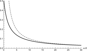
Figure 1: Plot for the auxiliary function ${\cal{F}}_{1}\left(mR\right)$ (solid line) defined in Eq. (42). The dashed line is the limiting function $1/mR$.

When we fix the distance between the charge and the mirror, from Eq. (39), we see that the whole system feels a torque depending on its orientation with respect to the background vector. In order to calculate this torque, we define as $0\leq\alpha\leq\pi$ the angle between the normal to the mirror and the background vector ${\bf{v}}$, in such a way that, ${\bf{v}}_{\parallel}^{2}={\bf{v}}^{2}\sin^{2}\left(\alpha\right)$. Thus the torque can be computed as follows,

$$\tau_{MC}=-\frac{\partial E_{MC}}{\partial\alpha}=\frac{q^{2}{\bf{v}}^{2}}{16\pi R}\sin\left(2\alpha\right)\left[\frac{1}{2}-mR+2\left(mR\right)^{2}e^{2mR}Ei\left(1,2mR\right)\right]\ .$$ (45)

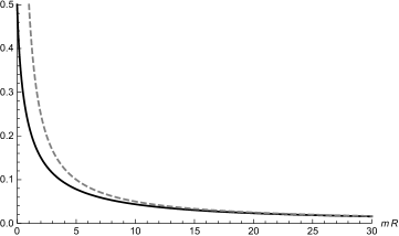
Figure 2: Plot for the auxiliary function ${\cal{F}}_{2}\left(mR\right)$ defined in Eq. (46). The dashed line is the limiting function $1/\left(2mR\right)$.

Equation (45) is a new effect with no counterpart in Maxwell electrodynamics in the presence of a semi-transparent mirror. For $\alpha=0,\pi/2,\pi$ the torque vanishes, while for $\alpha=\pi/4$ the torque exhibits a maximum absolute value. Defining the function

$${\cal{F}}_{2}\left(x\right)=\frac{1}{2}-{\cal Q}\left(x\right)$$ (46)

with

$${\cal Q}\left(x\right)=x-2x^{2}e^{2x}Ei\left(1,2x\right)\ ,$$

we can rewrite Eq. (45) in the form

$$\tau_{MC}=\frac{q^{2}{\bf{v}}^{2}}{16\pi R}\sin\left(2\alpha\right){\cal{F}}_{2}\left(mR\right)\ .$$ (47)

In Fig. (2), we show the behavior of ${\cal{F}}_{2}$ in terms of $mR$. This function is always positive, and goes to zero if $mR$ is large, with asymptotic behavior,

$${\cal{F}}_{2}\left(x\right)\underset{x\rightarrow\infty}{\sim}\frac{1}{2x}-\frac{3}{4x^{2}}+{\cal O}\left(\frac{1}{x^{3}}\right)\,.$$ (48)

It is well-known that the nonbirefringent components $k^{\mu\nu}$ can be divided in parity-even isotropic ${\tilde{\kappa}}_{\mathrm{tr}}$ component, anisotropic parity-even $\left({\tilde{\kappa}}_{e-}\right)^{ij}$ components and the parity-odd $\kappa^{i}$ components, which can be defined as follows

$$k^{00}=\frac{3}{2}{\tilde{\kappa}}_{\mathrm{tr}}\ \ ,\ k^{ij}=\frac{1}{2}{\tilde{\kappa}}_{tr}\delta^{ij}-\left({\tilde{\kappa}}_{e-}\right)^{ij}\ \ ,\ k^{0i}=-\kappa^{i}\ .$$ (49)

Now, the obtained results in (39), (43) and (47) can be written in terms of the above parameters by using the fact that,

$${\bf{v}}_{\parallel}^{2}-2\left(v^{0}\right)^{2}=-2{\tilde{\kappa}}_{\mathrm{tr}}-\left[\left({\tilde{\kappa}}_{e-}\right)^{11}+\left({\tilde{\kappa}}_{e-}\right)^{22}\right]\ \ ,\ \ {\bf{v}}^{2}=\frac{3}{2}{\tilde{\kappa}}_{\mathrm{tr}}\ .$$ (50)

It is clear from the graphic in Fig. (2) and Eq. (48) that, as $mR$ increases from zero to infinity, ${\cal{F}}_{2}$ decreases monotomically from $1/2$ to $0$, therefore

$$0\leq{\cal Q}\left(mR\right)\leq\frac{1}{2}\ .$$ (51)

This fact allows us to make some estimates on the value of ${\cal{F}}_{2}$ and, therefore, the torque, for reasonable values of the parameters in the theory. We consider a typical distance of atomic experiments in the vicinity of conductors (mirrors) of order $R\sim 10^{-6}$m, the fundamental electronic charge $q\sim 1.60217\times 10^{-19}\text{C}$, and the overestimated value ${\tilde{\kappa}}_{\mathrm{tr}}\sim 1.4\times 10^{-19}$ obtained from (FRKlin, ; VANR, ). In this case, for a perfect mirror, corresponding to the limit $m\rightarrow 0$, we have ${\cal Q}\left(mR\right)\rightarrow 0$ and ${\cal{F}}_{2}\rightarrow 1/2$. From Eq (47), we obtain a torque of order $\tau_{MC}\sim 10^{-41}\,\text{Nm}$. For an imperfect mirror, the magnitude of the torque is smaller. Taking $m\sim 10^{-5}\text{GeV}$, for example, we obtain $\tau_{MC}\sim 10^{-43}\,\text{Nm}$. This effect is out of reach of being measured by using current technology.

The model (4) can be considered as the electromagnetic version of the one studied in reference (LHCBAFFFAB, ), which is a Lorentz violating scalar field theory. As discussed in that reference, even in a Lorentz violation scenario it is always possible to relate some results obtained for a massless scalar field with the ones obtained in the corresponding electromagnetic model. For this task, in the electromagnetic results we must take $v^{0}=0$ and multiply by an overal factor of $-1$. In a scalar field theory the degree of transparency of the mirror has mass dimension +1 and therefore an opposite behavior in relation to the one studied here. However, the connection between the massless scalar field in the presence of a Dirichlet plane (perfect mirror) and the gauge field in the presence of a perfect conductor remains when we have the corresponding Lorentz violating terms in both theories. This fact can be clarified from Eq. (40), as follows

$$-\lim_{m\rightarrow 0}E_{MC}\left(v^{0}=0\right)=\frac{q^{2}}{16\pi R}\left(1+\frac{1}{2}{\bf{v}}_{\parallel}^{2}\right)\ ,$$ (52)

which is equal to Eq. (96) of (LHCBAFFFAB, ). The same connection can be observed in Lee-Wick electrodynamics (LW3, ).

IV Some results for more general LV background

In this section, we make some considerations regarding the generalization of our results for more general cases described by Eqs. (1) and (2). We start by defining,

$$f^{\prime}\left(v\right)={\bf{v}}_{\parallel}^{2}-2\left(v^{0}\right)^{2}\ ,$$ (53)

and rewriting Eq. (43) as follows,

$$F_{MC}=-\frac{q^{2}}{16\pi R^{2}}\Biggl{[}1-2mR+\left(2mR\right)^{2}e^{2mR}Ei\left(1,2mR\right)+f^{\prime}\left(v\right){\cal{F}}_{1}\left(mR\right)\Biggr{]}.$$ (54)

In the $m\rightarrow 0$ limit, we obtain the interaction force between the charge and the perfect mirror that was found in (LHCBFABplate, ) via the image method,

$$\lim_{m\rightarrow 0}F_{MC}=-\frac{q^{2}}{16\pi R^{2}}\left(1+\frac{1}{2}f^{\prime}\left(v\right)\right)\ .$$ (55)

In the general case of the model given in Eq. (1), we expect to find for the force an expression similar in form, but with a different function in place of $f^{\prime}$, i.e.,

$$F^{\prime}_{MC}=-\frac{q^{2}}{16\pi R^{2}}\Biggl{[}1-2mR+\left(2mR\right)^{2}e^{2mR}Ei\left(1,2mR\right)+f\left(K_{F}\right){\cal{F}}_{1}\left(mR\right)\Biggr{]},$$ (56)

where $f\left(K_{F}\right)$ is a function such that, given the particular choice defined in Eqs. (2) and (3), leads to $f\left(K_{F}\right)\rightarrow f^{\prime}\left(v\right)$. Similarly, in the $m\rightarrow 0$ we should have

$$\lim_{m\rightarrow 0}F^{\prime}_{MC}=-\frac{q^{2}}{16\pi R^{2}}\left(1+\frac{1}{2}f\left(K_{F}\right)\right)\ .$$ (57)

As we have discussed in (LHCBFABplate, ), the image method remains valid in that particular LV setting, and we assume the same happens here. This is a reasonable assumption, since one of the essential requirements for the application of the image method is the linearity of the equations of motion – which is preserved here – but not a completely trivial one, since another requirement is to have a sufficiently symmetric system. Lorentz violation evidently reduces the symmetry of the problem. However, the configuration discussed here is similar enough to the one treated in (LHCBFABplate, ) to give us confidence in using the image method for our considerations.

Thus, we consider that the result in Eq. (57) is equivalent to the interaction force, up to the first order in $K_{F}$, between two point charges $q_{1}=q$ and $q_{2}=-q$ separated by a distance $2R$. This result can be easily obtained from (fontes3, ) as

$$F_{CC}^{\prime}=-\frac{q^{2}}{16\pi R^{2}}\left[\left(K_{F}\right)^{0101}+\left(K_{F}\right)^{0202}\right],$$ (58)

where the $CC$ means this is the interaction force between two charges.

Comparing Eqs. (58) and (57), we obtain

$$f\left(K_{F}\right)=2\left[\left(K_{F}\right)^{0101}+\left(K_{F}\right)^{0202}\right]\ .$$ (59)

This indeed satisfy $f\left(K_{F}\right)\rightarrow f^{\prime}\left(v\right)$ in the particular case defined by Eqs. (2) and (3). It is therefore reasonable to expect that our results can be generalized by substituting $f^{\prime}\left(v\right)$ by $f\left(K_{F}\right)$ in the presence of a more generic LV background.

In terms of the LV parameters defined in (kosmat1, ; kosmat2, ), we have

$$\left(K_{F}\right)^{0101} =-\frac{1}{2}\left[\left({\tilde{\kappa}}_{e+}\right)^{11}+\left({\tilde{\kappa}}_{e-}\right)^{11}+{\tilde{\kappa}}_{\textrm{tr}}\right]\ ,$$ (60)

$$\left(K_{F}\right)^{0202} =-\frac{1}{2}\left[\left({\tilde{\kappa}}_{e+}\right)^{22}+\left({\tilde{\kappa}}_{e-}\right)^{22}+{\tilde{\kappa}}_{\textrm{tr}}\right]\ ,$$ (61)

leading to

$$f\left(K_{F}\right)=f^{\prime}\left(v\right)-\left[\left({\tilde{\kappa}}_{e+}\right)^{11}+\left({\tilde{\kappa}}_{e+}\right)^{22}\right]\ ,$$ (62)

where Eqs. (53) and (50) were taken into account.

Our conclusion is that, in a more general setting, our results will be modified by a contribution arising from the ${\tilde{\kappa}}_{e+}$ coefficients, as given in Eq. (62). So, for example, the interaction energy and force between the charge and the mirror will be

$$E_{MC}^{\prime} =E_{MC}+\frac{q^{2}}{16\pi R}\left[\left({\tilde{\kappa}}_{e+}\right)^{11}+\left({\tilde{\kappa}}_{e+}\right)^{22}\right]{\cal{F}}_{2}\left(mR\right)\ ,$$ (63)

$$F_{MC}^{\prime} =F_{MC}+\frac{q^{2}}{16\pi R^{2}}\left[\left({\tilde{\kappa}}_{e+}\right)^{11}+\left({\tilde{\kappa}}_{e+}\right)^{22}\right]{\cal{F}}_{1}\left(mR\right)\ ,$$ (64)

where $E_{MC}$ and $F_{MC}$ are given by Eqs. (39) and (43), respectively.

It is important to mention, however, that even if the $K_{F}$ tensor has nineteen independent components, just a subset of those can appear in the interaction that we are considering in this work.

Next, to obtain the resulting torque in the more general setting, it is convenient to write the interaction energy explicitly in terms of $K_{F}$,

$$E^{\prime}_{MC} =-\frac{q^{2}}{16\pi R}\Biggl{[}1-2mRe^{2mR}Ei\left(1,2mR\right)$$ (65)

$$+2\left[\left(K_{F}\right)^{0101}+\left(K_{F}\right)^{0202}\right]{\cal{F}}_{2}\left(mR\right)\Biggr{]}\ .$$ (66)

Defining a tree-dimensional vector

$${\bf{K}}_{F}=\left(\left(K_{F}\right)^{0101},\left(K_{F}\right)^{0202},\left(K_{F}\right)^{0303}\right)\ ,$$ (67)

we can write

$$\left(K_{F}\right)^{0101} =\mid{\bf{K}}_{F}\mid\sin\left(\theta\right)\cos\left(\phi\right)\ ,$$ (68)

$$\left(K_{F}\right)^{0202} =\mid{\bf{K}}_{F}\mid\sin\left(\theta\right)\sin\left(\phi\right)\ ,$$ (69)

where $0<\theta<\pi$ and $0<\phi<2\pi$ are the polar and azimuthal angles in spherical coordinates, respectively ($z$ being the polar axis). Substitution of Eq. (68) and (69) in Eq. (65) leads to

$$E^{\prime}_{MC}\left(\theta,\phi\right) =-\frac{q^{2}}{16\pi R}\Biggl{[}1-2mRe^{2mR}Ei\left(1,2mR\right)$$

$$+2\mid{\bf{K}}_{F}\mid\sin\left(\theta\right)\left[\cos\left(\phi\right)+\sin\left(\phi\right)\right]{\cal{F}}_{2}\left(mR\right)\Biggr{]}\ .$$ (70)

The interaction energy in Eq. (70) generates two kind of torques on the system, depending on its orientation with regards to the background LV, one related to the $\theta$ angle, and another to the $\phi$ angle, i.e.,

$$\tau^{\prime}_{MC}\left(\theta\right) =-\frac{\partial}{\partial\theta}E^{\prime}_{MC}\left(\theta,\phi\right)$$

$$=\frac{q^{2}}{8\pi R}\mid{\bf{K}}_{F}\mid\cos\left(\theta\right)\left[\cos\left(\phi\right)+\sin\left(\phi\right)\right]{\cal{F}}_{2}\left(mR\right)\ ,$$ (71)

and

$$\tau^{\prime}_{MC}\left(\phi\right) =-\frac{\partial}{\partial\phi}E^{\prime}_{MC}\left(\theta,\phi\right)$$

$$=\frac{q^{2}}{8\pi R}\mid{\bf{K}}_{F}\mid\sin\left(\theta\right)\left[\cos\left(\phi\right)-\sin\left(\phi\right)\right]{\cal{F}}_{2}\left(mR\right)\ .$$ (72)

In order to make an estimation on these torques, we have to write $\mid{\bf{K}}_{F}\mid$ in terms of the usual LV coefficients, using Eqs. (60) and (61), together with

$$\mid{\bf{K}}_{F}\mid=\Bigl{\{}\left[\left(K_{F}\right)^{0101}\right]^{2}+\left[\left(K_{F}\right)^{0202}\right]^{2}+\left[\left(K_{F}\right)^{0303}\right]^{2}\Bigr{\}}^{1/2}$$ (73)

thus obtaining

$$\left(K_{F}\right)^{0303}=-\frac{1}{2}\left[\left({\tilde{\kappa}}_{e+}\right)^{33}+\left({\tilde{\kappa}}_{e-}\right)^{33}+{\tilde{\kappa}}_{\textrm{tr}}\right]\ .$$ (74)

Using the same data we considered in the last section, together with the upper bounds $\left({\tilde{\kappa}}_{e-}\right)^{ij}\sim 4\times 10^{-18}$ and $\left({\tilde{\kappa}}_{e+}\right)^{ij}\sim 2\times 10^{-37}$ from (VANR, ), we obtain an order of magnitude estimate of $\tau^{\prime}_{MC}\sim 10^{-40}$Nm for a perfect mirror, and $\tau^{\prime}_{MC}\sim 10^{-45}$Nm for $m\sim 10^{-5}$GeV.

As a final note, we mention that obtaining the results of this section through an explicit calculation, as done in Sec. III, would not be a possible task, since the propagators would be much more involved, and the resulting integrals would result too complicated to be calculated analytically. The results we present here, however, are founded on the explicit results obtained in the previous section for the particular case, as well as the application of the image method, which has been extensively discussed in a similar setting in (LHCBFABplate, ).

V Conclusions and final remarks

In this paper we have studied some aspects of the nonbirefringent CPT-even gauge sector of the SME near a semi-transparent mirror. We considered a model where the Lorentz symmetry breaking is caused by a single background vector $v^{\mu}$ and obtained perturbative results up to second order in this parameter.

We computed the modified Lorentz violating propagator for the gauge field due to presence of the mirror and calculated the interaction energy, as well as the interaction force, between the mirror and a static point-like charge. In the limiting case of perfect mirrors, we recovered the interaction found via the image method.

We showed that when the charge is placed in the vicinity of the mirror, a spontaneous torque emerges on this system due to the orientation of the mirror with respect to the LV background vector. This torque is a new effect with no counterpart in Maxwell electrodynamics in the presence of a semi-transparent mirror. We also showed that the connection between the massless scalar field in the presence of a Dirichlet plane and the gauge field in the presence of a perfect conductor remains when we have the corresponding Lorentz violating terms in both theories.

Then, we used the image method to generalize our results for a more general Lorentz violating $K_{F}$ coefficient. We were able to obtain some estimates for the physical effects that it can induce in the interaction of a point-like charge and a mirror.

As a possible future study, one interesting point would be the inclusion of the CPT-odd photon sector of the SME, in the presence of semi-transparent boundaries (inprep, ).

Acknowledgments. This study was financed in part by the Coordenação de Aperfeiçoamento de Pessoal de Nível Superior – Brasil (CAPES) – Finance Code 001 (LHCB), and Conselho Nacional de Desenvolvimento Científico e Tecnológico (CNPq) via the grant 305967/2020-7 (AFF).

References

• (1) D. Colladay, V. A. Kostelecký, Phys. Rev. D 55, 6760 (1997).
• (2) D. Colladay, V. A. Kostelecký, Phys. Rev. D 58, 116002 (1998).
• (3) L.H.C. Borges, F.A. Barone, J. A. Helayel-Neto, Eur. Phys. J. C 74, 2937 (2014).
• (4) L. H. C. Borges, A. F. Ferrari, F. A. Barone, Eur. Phys. J. C 76, 599 (2016).
• (5) L.H.C. Borges, F.A. Barone, Braz. J. Phys. 49, 571-582 (2019).
• (6) H. Belich, M.M. Ferreira, J.A. Helayel-Neto and M.T.D. Orlando, Phys. Rev. D 68, 025005 (2003).
• (7) Q.G. Bailey and V.A. Kostelecký, Phys. Rev. D 70, 076006 (2004).
• (8) Rodolfo Casana, Manoel M. Ferreira Jr., Adalto R. Gomes, and Frederico E. P. dos Santos, Phys. Rev. D 82, 125006 (2010).
• (9) Rodolfo Casana, Manoel M. Ferreira Jr., Adalto R. Gomes, and Paulo R. D. Pinheiro Phys. Rev. D 80, 125040 (2009).
• (10) Rodolfo Casana, Manoel M. Ferreira Jr, and Carlos E. H. Santos, Phys. Rev. D 78, 105014 (2008).
• (11) L.H.C. Borges, F.A. Barone, A.F. Ferrari, Europhys. Lett. 122, 31002 (2018).
• (12) Manoel M. Ferreira Jr., Letí cia Lisboa-Santos, Roberto V. Maluf, and Marco Schreck, Phys. Rev. D 100, 055036 (2019).
• (13) Rodolfo Casana, Manoel M. Ferreira Jr., Letícia Lisboa-Santos, Frederico E. P. dos Santos, Marco Schreck, Phys. Rev. D 97, 115043 (2018).
• (14) L.H.C. Borges and A.F. Ferrari, Mod.Phys.Lett.A 37 (2022) 04, 2250021.
• (15) F.R. Klinkhamer and M. Schreck, Nuc. Phys. B 848, 90 (2011).
• (16) M.A. Hohensee, R. Lehnert, D.F. Phillips and R.L. Walsworth, Phys. Rev. D 80, 036010 (2009).
• (17) D. Colladay and V.A. Kostelecký, Phys. Lett. B 511, 209 (2001).
• (18) B. Charneski, M. Gomes, R.V. Maluf, and A. J. da Silva, Phys. Rev. D 86, 045003 (2012).
• (19) G.P. de Brito, J.T. Guaitolini Junior, D. Kroff, P.C. Malta, and C. Marques, Phys. Rev. D 94, 056005 (2016).
• (20) Frederico E.P. dos Santos and Manoel M. Ferreira, Symmetry 10, 302 (2018).
• (21) J.C.C. Felipe, H.G. Fargnoli, A.P. Baeta Scarpelli, and L.C.T. Brito, Int. Jour. of Mod. Phys. A 34, 1950139 (2019).
• (22) A.J.G. Carvalho, A.F. Ferrari, A.M. de Lima, J.R. Nascimento, A. Yu. Petrov, Nucl. Phys. B 942, 393-409 (2019).
• (23) R. Jackiw and V.A. Kostelecký, Phys. Rev. Lett. 82, 3572 (1999).
• (24) A.P. Baêta Scarpelli, M. Sampaio, M.C. Nemes, and B. Hiller, Eur. Phys. J. C 56, 571 (2008).
• (25) J.R. Nascimento, E. Passos, A.Yu. Petrov, and F.A. Brito, JHEP 0706, 016 (2007).
• (26) T. Mariz, J.R. Nascimento, E. Passos, R.F. Ribeiro, and F.A. Brito, JHEP 0510, 019 (2005).
• (27) M. Pérez-Victoria, JHEP 0104, 032 (2001).
• (28) G. Bonneau, Nucl. Phys. B 593, 398 (2001).
• (29) B. Altschul, Phys. Rev. D 99, 111701(R) (2019).
• (30) L.H.C. Borges, A.G. Dias, A.F. Ferrari, J.R. Nascimento, A. Yu. Petrov, Phys. Rev. D 89, 045005 (2014).
• (31) A. F. Ferrari, J. R. Nascimento, A. Yu. Petrov, Eur. Phys. J. C 80, 459 (2020).
• (32) A. de Souza Dutra, M. Hott, and F.A. Barone, Phys. Rev. D 74, 085030 (2006).
• (33) M.N. Barreto, D. Bazeia, and R. Menezes, Phys. Rev. D 73, 065015 (2006).
• (34) A. de Souza Dutra, and R.A.C. Correa, Phys. Rev. D 83, 105007 (2011).
• (35) R. Casana, M.M. Ferreira Jr., E. da Hora, and A.B.F. Neves, Eur. Phys. J. C 74, 3064 (2014).
• (36) L.H.C. Borges, A.G. Dias, A.F. Ferrari, J.R. Nascimento, A.Yu. Petrov, Phys. Lett. B 756, 332 (2016).
• (37) B. Agostini, F.A. Barone, F.E. Barone, Patricio Gaete, J. A. Helayel-Neto, Phys. Lett. B 708, 212 (2012).
• (38) L.H.C. Borges and D. Dalmazi, Phys. Rev. D 99, 024040 (2019).
• (39) R. Jackiw and S. Y. Pi, Phys. Rev. D 68, 104012 (2003).
• (40) A. F. Ferrari, M. Gomes, J. R. Nascimento, E. Passos, A. Yu. Petrov, A. J. da Silva, Phys. Lett. B 652, 174-180 (2007).
• (41) B. Pereira-Dias, C. A. Hernaski and J. A. Helayel-Neto, Phys. Rev. D 83, 084011 (2011).
• (42) R. V. Maluf, C. A. S. Almeida, R. Casana, M. M. Ferreira Jr., Phys. Rev. D 90, 025007 (2014).
• (43) V. Alan Kostelecký and Matthew Mewes, Phys. Lett. B 757, 510-514 (2016).
• (44) V. Alan Kostelecký and Matthew Mewes, Phys. Lett. B 779, 136-142 (2018).
• (45) A. Anisimov, T. Banks, M. Dine, M. Graesser, Phys. Rev. D 65, 085032 (2002).
• (46) C.E. Carlson, C.D. Carone, R.F. Lebed, Phys. Lett. B 518, 201 (2001).
• (47) S. Aghababaei and M. Haghighat Phys. Rev. D 96, 075017 (2017).
• (48) K.A. Milton, The Casimir Effect, Physical Manifestations of Zero-Point Energy, World Scientific, Singapore (2001).
• (49) M. Bordag, U. Mohideen, and V. M. Mostepanenko, Phys. Rep. 353, 1 (2001).
• (50) Kimball A. Milton, J. Phys. A: Math. Gen.37, 63916406 (2004).
• (51) M. Bordag, K. Kirsten and D. Vassilevich, Phys. Rev. D 59, 085011 (1999).
• (52) N. Graham, R.L. Jaffe, V. Khemani, M. Quandt, M. Scandurra and H. Weigel, Nucl. Phys. B 645, 49 (2002).
• (53) N. Graham, R.L. Jaffe, V. Khemani, M. Quandt, M. Scandurra and H. Weigel, Phys. Lett. B 572, 196 (2003).
• (54) P. Sundberg and R.L. Jaffe, Annals Phys. 309, 442 (2004).
• (55) R.M. Cavalcanti, [arXiv:hep-th/0201150].
• (56) F. A. Barone and F. E. Barone, Eur. Phys. J. C 74, 3113 (2014).
• (57) F.A. Barone and F.E. Barone, Phys. Rev. D 89, 065020 (2014).
• (58) G. T. Camilo, F. A. Barone and F. E. Barone, Phys. Rev. D 87, 025011 (2013).
• (59) H.L. Oliveira, L.H.C. Borges, F.E. Barone and F.A. Barone, Eur. Phys. J. C 81, 558 (2021).
• (60) F. A. Barone and A. A. Nogueira, Eur. Phys. J. C 75, 339 (2015).
• (61) F.A. Barone and A.A. Nogueira, Int. J. Mod. Phys.: Conf. Ser. 41, 1660134, (2016).
• (62) M. Blazhyevska, J. of Phys. Stud. 16, 3001 (2012).
• (63) L.H.C. Borges, A.A. Nogueira, E.H. Rodrigues, F.A. Barone, Eur. Phys. J. C 80, 1082 (2020).
• (64) L. H. C. Borges, F. E. Barone, C. C. H. Ribeiro, H. L. Oliveira, R. L. Fernandes, F. A. Barone, Eur. Phys. J. C 80, 238 (2020).
• (65) L.H.C. Borges and F.A. Barone, Phys. Lett. B 824, 136759 (2022).
• (66) M.B. Cruz, E.R. Bezerra de Mello and A. Yu. Petrov, Phys. Rev. D 96, 045019 (2017).
• (67) M.B. Cruz, E.R. Bezerra de Mello and A. Yu. Petrov, Mod. Phys. Lett. A 33, 1850115 (2018).
• (68) M. Frank, I. Turan, Phys. Rev. D 74, 033016 (2006).
• (69) A.F. Santos, F.C. Khanna, Phys. Lett. B 762, 283 (2016).
• (70) L. M. Silva, H. Belich, J. A. Helayel-Neto, arXiv:1605.02388 (2016).
• (71) A. Martí n-Ruiz, C.A. Escobar, Phys. Rev. D 94, 076010 (2016).
• (72) Dêivid R. da Silva and E. R. Bezerra de Mello, arXiv:2006.12924 (2020).
• (73) A. Martí n-Ruiz, C.A. Escobar, A.M. Escobar-Ruiz, and O.J. Franca, Phys. Rev. D 102, 015027 (2020).
• (74) Amirhosein Mojavezi, Reza Moazzemi, Mohammad Ebrahim Zomorrodian, Nucl. Phys. B 941, 145-157 (2019).
• (75) M.B. Cruz, E.R. Bezerra de Mello, and A. Yu. Petrov, Phys. Rev. D 99, 085012 (2019).
• (76) C. A. Escobar, Leonardo Medel, and A. Martí n-Ruiz, Phys. Rev. D 101, 095011 (2020).
• (77) Andrea Erdas, arXiv:2005.07830 (2020).
• (78) M.A. Valuyan, Mod. Phys. Lett. A 35, 2050149 (2020).
• (79) M.B. Cruz, E.R. Bezerra de Mello, and H. F. Santana Mota, Phys. Rev. D 102, 045006 (2020).
• (80) Massimo Blasone, Gaetano Lambiase, Luciano Petruzziello, and Antonio Stabile, Eur. Phys. J. C 78, 976 (2018).
• (81) L.H.C. Borges and F.A. Barone, Eur. Phys. J. C 77, 693 (2017).
• (82) L.H.C. Borges and F.A. Barone, Braz. J. Phys. 50, 647-657 (2020).
• (83) L. H. C. Borges, A. F. Ferrari and F. A. Barone, Nucl. Phys. B 954, 114974 (2020).
• (84) L.H.C. Borges and F.A. Barone, Eur. Phys. J. C 76, 64 (2016).
• (85) B. Altschul, Phys. Rev. Lett. 98, 041603 (2007).
• (86) I.S. Gradshteyn and I.M. Ryzhik, Table of Integrals, Series, and Products, Academic Press (2000).
• (87) G.B. Arfken, H.J. Weber, Mathematical Methods for Physicists (Academic Press, USA, 1995).
• (88) F.R. Klinkhamer and M. Risse, Phys. Rev. D 77, 117901 (2008).
• (89) V.A. Kostelecký, N. Russell. arXiv:0801.0287v15 (2022).
• (90) V. A. Kostelecký and M. Mewes, Phys. Rev. Lett. 87, 251304 (2001).
• (91) V. A. Kostelecký and M. Mewes, Phys. Rev. D 66, 056005 (2002).
• (92) L. H. C. Borges, A. F. Ferrari, in preparation.