Frozen-Density Embedding for including environmental effects in the Dirac-Kohn-Sham theory: an implementation based on density fitting and prototyping techniques

Abstract

The Frozen Density Embedding (FDE) scheme represents an embedding method in which environmental effects onto a given subsystem are included by representing the other subsystems making up the surroundings quantum mechanically, by means of their electron densities. In the present paper, we extend the full 4-component relativistic Dirac-Kohn-Sham (DKS) method, as implemented in the BERTHA code, to include environmental and confinement effects with the FDE scheme (DKS-in-DFT FDE). This implementation has been enormously facilitated by BERTHA’s python API (PyBERTHA), which provides a flexible framework of development by using all Python advantages in terms of code re-usability, portability while facilitating the interoperability with other FDE implementations available through the PyADF framework. The accuracy and numerical stability of this new implementation, also using different auxiliary fitting basis sets, has been demonstrated on the simple NH₃-H₂O system in comparison with a reference non relativistic implementation. The computational performance has been evaluated on a series of gold clusters (Au_n, with $n=2,4,8$) embedded into an increasing number of water molecules (5, 10, 20, 40 and 80 water molecules). We found that the procedure scales approximately linearly both with the size of the frozen surrounding environment (in line with the underpinnings of the FDE approach) and with the size of the active system (in line with the use of density fitting). Finally, we applied the code to a series of Heavy (Rn) and Super-Heavy elements (Cn, Fl, Og) embedded in a C₆₀ cage to explore the confinement effect induced by C₆₀ on their electronic structure. We compare the results from our simulations with more approximate models employed in the atomic physics literature, in which confinement is represented by a radial potential slightly affected by the nature of the central atom. Our results indicate that the specific interactions described by FDE are able to improve upon the cruder approximations currently employed, and thus provide a basis from which to generate more realistic radial potentials for confined atoms.

1 Introduction

Molecular systems, clusters, and materials containing heavy atoms have drawn considerable recent attention because of their rich chemistry and physics^{1, 2, 3, 4}. In order to model computationally systems containing heavy elements, the methods of relativistic quantum mechanics must be necessarily adopted to capture scalar and spin-orbit interactions that are neglected in the conventional non-relativistic formulation of quantum chemistry. Furthermore, most of the chemistry occurs in solution and the environment plays a key role in the determination of the properties and reactivity of substances in condensed phases^{5, 6, 7, 8, 9}. Thus, the complexity of chemical phenomena in solution has made it necessary to develop a variety of models and computational techniques to be combined with (relativistic) quantum chemistry methods. Among different approaches to include environmental effects we mention the quantum mechanics/molecular mechanics (QM/MM) approach ¹⁰, which includes the molecular environment explicitly and at a reduced cost using classical mechanical description, or in polarizable continuous medium (PCM)¹¹ (i.e., where the solvent degree of freedom are replaced by an effective classical dielectric). Despite being widely and successfully applied these methods may have drawbacks. For instance methods based on PCM cannot describe specific interactions with the environments (e.g. hydrogen, halogen bonds), while the QM/MM approach, which is based on classical force fields, may be limited by the availability of accurate parameterizations which may reduce its predictive power, in particular when heavy elements are involved. An alternative is to use quantum embedding theories (for an overview see Ref.12, 13, 14, 15 and references therein), in which a QM description for a subsystem of interest is combined with a QM description of the environment (QM/QM). A notable example of QM/QM methods is the frozen-density embedding (FDE) scheme introduced by Wesołowski and Warshel,^{16, 17} based on the approach originally proposed by Senatore and Subbaswamy ¹⁸, and later Cortona ¹⁹, for solid-state calculations. The method has been further generalized ^{20, 21} and directed to the simultaneous optimization of the subsystems electronic densities.

FDE is a DFT-in-DFT embedding method that allows to partition a larger Kohn-Sham system into a set of smaller, and coupled, Kohn-Sham subsystems. The coupling term is defined by a local embedding potential depending only on the electron densities of both the sole active subsystem and the environment (i.e. no orbital information is shared among subsystems). This feature gives to the FDE scheme an enormous flexibility, as indeed virtually arbitrary methods can be combined to treat different subsystems. For example, wavefunction theory (WFT) based methods can be used for the active system while one can take advantage of the efficiency of DFT to describe a large environment (WFT-in-DFT) ^{22, 23, 24, 12, 13, 25, 17}. Also one can employ very different computational protocols for different subsystem including i) using Hamiltonian dealing with different relativistic approximations (from the full 4-component methods to the non-relativistic ones) ^{26, 27, 28, 29}; ii) different basis sets size and type (Gaussian and Slater type functions, relativistic four-component spinors) and even iii) different quantum chemical packages^{26, 30, 31}. We mention that the FDE scheme has been extended both to the linear-response TDDFT ^{32, 33, 34}, including to account for charge-transfer excitations ^{35, 36} and to real time TDDFT (rt-TDDFT).^{37, 31}

FDE-based calculations are shown to be accurate in the case of weakly interacting systems including hydrogen bond systems^{38, 39}, whereas, their use for subsystems interacting with a larger covalent character is problematic (see Ref.38 and references therein) due to the use of approximate kinetic energy functional (KEDF) in the non-additive contribution to the embedding potential. The research for more accurate KEDFs is a key aspect for the applicability of the FDE scheme as a general scheme ^{40, 41, 42, 43}, including the partitioning of the system also breaking covalent bonds. ⁴⁴ We mention here that alternative QM/QM approaches, avoiding the use of KEDFs and allowing also for fragmentation in subsystems through covalent bonds, have been recently proposed (see for instance Ref.^{45, 46, 47, 48, 49, 14, 50, 15, 51}).

Thanks to its flexibility the FDE scheme has been implemented in different flavors into computational packages such as: embedded Quantum Espresso⁵², ADF^{53, 21, 54}, Turbomole ^{55, 56}, Dalton ^{26, 57}, Koala ⁵⁸, Molpro ⁴⁵, Serenity⁵⁹, and Q-Chem ⁶⁰, (the first two based on plane waves and Slater type functions respectively, the others on Gaussian type functions). FDE has also been implemented to treat the subsystems at full-relativistic four-component level based on the Dirac equation within the DIRAC code⁶¹, and can be used with DFT and different wavefunction methods both for molecular properties and energies involving the ground or excited electronic states ^{26, 62, 63, 28, 64, 29}.

Despite its conceptual simplicity, its actual implementations may lead to relatively complicated workflows. A simpler approach is therefore to integrate such legacy codes as computational engines to handle the different FDE steps, which are then glued together and their execution automatized using suitable frameworks such as for instance that implemented in PyADF ^{30, 65}, that can be easily extensible due to its object-oriented implementation in the Python programming language ⁶⁶. Prototyping techniques also based on Python are very useful to build reference implementations, as for instance the Psi4-rt-PyEmbed code^{31, 67}, where the Python interface of Psi4Numpy and PyADF ^{30, 68} (including its PyEmbed module^{69, 70} and XCFun library^{71, 72} to evaluate non-additive exchange-correlation and kinetic energy contributions) has been used by some of us to build real time non-relativistic TDDFT-in-DFT FDE ³¹ and projection-based embedding⁷³ implementations.

In this work we extend the Dirac-Kohn-Sham (DKS) method implemented in the BERTHA code (with its new Python API, PyBERTHA)^{74, 75} to the FDE scheme to include environmental/confinement effects in the DKS calculations (DKS-in-DFT FDE). The implementation takes advantages of the DKS formulation implemented in BERTHA, including the density fitting algorithms at the core of the computation (i.e. in the evaluation of the embedding potential and of its matrix representation is relativistic G-spinor functions), and the FDE implementation already available in the PyEmbed module of the PyADF framework.

The outline of the paper is as follows. In Section 2 we present the basic theory of FDE and a brief description of the DKS method as implemented in BERTHA. In section 3, we then describe in detail our implementation. In section 4 we present some numerical results, including the computational burden and scalability of this new implementation with respect to the size of the active system as well as of the embedding one. We will also present an application to a series of Heavy (Rn) and Super-Heavy elements (Cn, Fl, Og) confined into a C₆₀ cage. Finally, concluding remarks are given in section 5.

2 Theory

In this section, we briefly review the basic formalism of the FDE scheme and its extension to use the DKS theory for the active system (DKS-in-DFT FDE). We will remark also some details of the DKS implementation in BERTHA, mainly focusing on those aspects (including density fitting techniques), which are relevant for an efficient implementation of the FDE scheme. Finally, we will illustrate the basic characteristics of the our recent BERTHA Python API, PyBERTHA (and the related pyberthamod module available under GPLv3 license at Ref.67, for additional and technical details see Refs.76, 74, 75) which is a key tool here to devise a simple work-flow for the DKS-in-DFT FDE scheme.

2.1 Subsystem DFT and Frozen Density Embedding formulation

In the subsystem formulation of DFT the entire system is partitioned into N subsystems, and the total density $\rho_{\text{tot}}(\bm{r})$ is represented as the sum of electron densities of the various subsystems [i.e., $\rho_{a}(\bm{r})$ ($a=I,..,N$)]. In the following we consider the total density as partitioned in only two contributions as

$$\rho_{\text{tot}}(\bm{r})=\rho_{\text{I}}(\bm{r})+\rho_{\text{II}}(\bm{r}).$$ (1)

The total energy of the system can then be written as

$$E_{\text{tot}}[\rho_{\text{I}},\rho_{\text{II}}]=E_{\text{I}}[\rho_{\text{I}}]+E_{\text{II}}[\rho_{\text{II}}]+E_{\text{int}}[\rho_{\text{I}},\rho_{\text{II}}]$$ (2)

with the energy of each subsystem ($E_{i}[\rho_{i}]$, with $i=\text{I},\text{II}$) given according to the usual definition in DFT as

$$E_{i}[\rho_{i}] =\int\rho_{i}(\bm{r})v_{\text{nuc}}^{i}(\bm{r}){\rm d}^{3}r+\frac{1}{2}\iint\frac{\rho_{i}(\bm{r})\rho_{i}(\bm{r}^{\prime})}{|\bm{r}-\bm{r}^{\prime}|}{\rm d}^{3}r{\rm d}^{3}r^{\prime}+$$ (3)

$$+E_{\text{xc}}[\rho_{i}]+T_{s}[\rho_{i}]+E_{\text{nuc}}^{i}.$$

In the above expression, $v_{\text{nuc}}^{i}(\bm{r})$ is the nuclear potential due to the set of atoms which defines the subsystem, and $E_{\text{nuc}}^{i}$ is the related nuclear repulsion energy. $T_{s}[\rho_{i}]$ is the kinetic energy of the auxiliary non-interacting system, which is, within the Kohn-Sham (KS) approach, commonly evaluated using the KS orbitals. The interaction energy is given by the expression:

$$E_{\text{int}}[\rho_{\text{I}},\rho_{\text{II}}] =\int\rho_{\text{I}}(\bm{r})v_{\text{nuc}}^{\text{II}}(\bm{r}){\rm d}^{3}r+\int\rho_{\text{II}}(\bm{r})v_{\text{nuc}}^{\text{I}}(\bm{r}){\rm d}^{3}r+E^{\text{I,II}}_{\text{nuc}}$$ (4)

$$+\iint\frac{\rho_{\text{I}}(\bm{r})\rho_{\text{II}}(\bm{r}^{\prime})}{|\bm{r}-\bm{r}^{\prime}|}{\rm d}^{3}r{\rm d}^{3}r^{\prime}+E^{\text{nadd}}_{\text{xc}}[\rho_{\text{I}},\rho_{\text{II}}]+T^{\text{nadd}}_{s}[\rho_{\text{I}},\rho_{\text{II}}]$$

with $v_{\text{nuc}}^{\text{I}}$ and $v_{\text{nuc}}^{\text{II}}$ being the nuclear potentials due to the set of atoms associated with the subsystem I and II, respectively. The repulsion energy for nuclei belonging to different subsystems is described by the $E^{\text{I,II}}_{\text{nuc}}$ term. The non-additive contributions ($E^{\text{nadd}}_{\text{xc}}[\rho_{\text{I}},\rho_{\text{II}}]$ and $T^{\text{nadd}}_{s}[\rho_{\text{I}},\rho_{\text{II}}])$ arise because both exchange-correlation and kinetic energy, in contrast to the Coulomb interaction, are not linear functionals of the density.

The electron density of a given fragment ($\rho_{\text{I}}$ or $\rho_{\text{II}}$ in this case) can be determined by minimizing the total energy functional (Eq.2) with respect to the density of the fragment while keeping the density of the other subsystem frozen. This procedure is the essence of the FDE scheme and leads to a set of Kohn-Sham-like equations (one for each subsystem)

$$\Big{[}\mathcal{T}+v^{\text{KS}}_{\text{eff}}[\rho_{\text{I}}](\bm{r})+v_{\text{emb}}^{\text{I}}[\rho_{\text{I}},\rho_{\text{II}}](\bm{r})\Big{]}\phi_{k}^{\text{I}}(\bm{r})=\varepsilon_{k}^{\text{I}}\phi_{k}^{\text{I}}(\bm{r}).$$ (5)

which are coupled by the embedding potential term $v^{\text{I}}_{\text{emb}}(\bm{r})$, which carries all dependence on the other fragment’s density. Here $\mathcal{T}$ denotes the kinetic energy operator, which in a non-relativistic framework has the form $-\nabla^{2}/2$, whereas for a relativistic framework is $c\bm{\alpha}\cdot{\bf p}$ (see discussion below). We also note that in the relativistic framework, the FDE expressions above correspond to the case in which an external vector potential is absent. Further details for their generalization can be found in Ref. 28.

In this equation, $v^{\text{KS}}_{\text{eff}}[\rho_{\text{I}}](\bm{r})$ is the KS potential calculated on basis of the density of subsystem I only, whereas $v_{\text{emb}}^{\text{I}}[\rho_{\text{I}},\rho_{\text{II}}](\bm{r})$ is the embedding potential that takes into account the effect of the other subsystem (which we consider here as the complete environment). In the framework of FDE theory, $v^{\text{I}}_{\text{emb}}(\bm{r})$ is explicitly given by

$$v^{\text{I}}_{\text{emb}}[\rho_{\text{I}},\rho_{\text{II}}](\bm{r})=\frac{\delta E_{\text{int}}[\rho_{\text{I}},\rho_{\text{II}}]}{\delta\rho_{\text{I}}(\bm{r})}= \ v_{\text{nuc}}^{\text{II}}(\bm{r})+\int\frac{\rho_{\text{II}}(\bm{r}^{\prime})}{|\bm{r}-\bm{r}^{\prime}|}{\rm d}^{3}r^{\prime}+\frac{\delta E_{\text{xc}}^{\text{nadd}}[\rho_{\text{I}},\rho_{\text{II}}]}{\delta\rho_{\text{I}}(\bm{r})}+\frac{\delta T^{\text{nadd}}_{s}[\rho_{\text{I}},\rho_{\text{II}}]}{\delta\rho_{\text{I}}(\bm{r})},$$ (6)

where the non-additive exchange-correlation and kinetic energy contributions are defined as the difference between the associated exchange-correlation and the kinetic potentials defined using $\rho_{\text{tot}}(\bm{r})$ (i.e., $\rho_{\text{I}}(\bm{r})+\rho_{\text{II}}(\bm{r})$) and $\rho_{\text{I}}(\bm{r})$. For both potentials one needs to account for the fact that only the density is known for the total system, so that potentials that require input in the form of KS orbitals are prohibited. For the exchange-correlation potential, one may make use of accurate density functional approximations and its quality is therefore similar to that of ordinary KS. The potential for the non-additive kinetic term ($\frac{\delta T^{\text{nadd}}_{s}[\rho]}{\delta\rho_{\text{I}}(\bm{r})}$, in Eq.6) is more problematic as less accurate orbital-free kinetic energy density functionals (KEDFs) are available for this purpose. Examples of popular functional approximations applied in this context are the Thomas-Fermi (TF) kinetic energy functional⁷⁷ or the GGA functional PW91k⁷⁸. As already mentioned in the introduction, the research for more accurate KEDFs is a key aspect for the applicability of the FDE scheme as a general scheme, including the partitioning of the system also breaking covalent bonds.⁴⁴

In general, the set of coupled equations that arise in the FDE scheme for the subsystems have to be solved iteratively and a freeze-and-thaw scheme, where one relaxes the electron density of one subsystem at a time keeping frozen the others, until electron densities of all subsystems reach a required convergence. In this work we limit to one subsystem (active) while keeping the density of the environment frozen to their ground state density. In this case, the implementation of FDE reduces to the evaluation of $v^{\text{I}}_{\text{emb}}(\bm{r})$ potential (which is an one-electron operator) that needs to be added to the Hamiltonian of the active system. The matrix representation of the embedding potential may be evaluated using numerical integration grids, similar to those used for the exchange-correlation term in the KS method. This contribution is then added to the KS matrix and the eigenvalue problem is solved with the usual self-consistent field (SCF) procedure. We note here that two approaches can be taken: the first is the use of a pre-calculated embedding potential ²⁶ (for instance, from a prior subsystem DFT calculation) that is used as a one-body operator (referred to in the literature as a “static” embedding potential) added to the one-body Fock matrix at the start of the (4-component) calculations. The second approach involves the regeneration of the embedding potential using the (4-component) actual electron density of the active system. In this case, the matrix representation of the embedding potential is updated during SCF procedure, because of its dependence on the active subsystem density (see Eq.6) that itself changes during the SCF iterations. As discussed below, in this work we shall mostly make use of the latter approach.

2.2 Dirac-Kohn-Sham scheme in BERTHA and its extension to FDE based on density fitting

For the detailed theoretical basis of the Dirac-Kohn-Sham methodology we refer the reader to previous works^{79, 80, 81, 82, 83, 84, 85} and references therein. Here, we summarize only the main aspects of the implementation of an all-electron DKS method based on the use of G-spinor basis sets and the density-fitting techniques as is implemented in BERTHA^{86, 75}. In atomic units, and including only the longitudinal electrostatic potential, the DKS equation reads

$$\{c\bm{\alpha}\cdot{\bf p}+{\beta}c^{2}+v^{(l)}({\bf r})\}{\bm{\Psi}}_{i}({\bf r})=\varepsilon_{i}{\bm{\Psi}}_{i}({\bf r}),$$ (7)

where $c$ is the speed of light in vacuum, $\bf p$ is the electron momentum, while:

$${\bm{\alpha}}=\left(\begin{array}[]{cc}0&{\bm{\sigma}}\\ {\bm{\sigma}}&0\end{array}\right)\ \mbox{and}\ {\bm{\beta}}=\left(\begin{array}[]{cc}{\bm{I}}&0\\ 0&-{\bm{I}}\end{array}\right)$$ (8)

where ${\bm{\sigma}}=(\sigma_{x},\sigma_{y},\sigma_{z})$, $\sigma_{q}$ is a $2\times 2$ Pauli spin matrix and ${\bm{I}}$ is the $2\times 2$ identity matrix. The longitudinal interaction term is represented by a diagonal operator borrowed from non-relativistic theory and made up of: a nuclear potential term $v_{\mathrm{N}}(\bm{r})$, a Coulomb interaction term $v^{(l)}_{\mathrm{H}}[\rho(\bm{r})]$, and the exchange-correlation term $v^{(l)}_{\mathrm{XC}}[\rho(\bm{r})]$. We mention that the Breit interaction contributes to the transverse part of the Hartree interaction and is not considered here, as we restrict ourselves to using non-hybrid, non-relativistic functionals of the electron density.

In BERTHA, the spinor solution (${\bm{\Psi}}_{i}({\bf r})$ in Eq. 7) is expressed as a linear combination of the G-spinor basis functions ⁸⁷, $M_{\mu}^{T}(\bm{r})$ ($T=L,S$ with $L$ and $S$ refer to the so-called “large” and “small” component, respectively). The G-spinors do not suffer from the variational problems of kinetic balance (see Ref. 88 and references therein) and, regarding the evaluation of multicentre integrals, retain the advantages that have made Gaussian-type functions the most widely-used expansion set in non-relativistic quantum chemistry. The matrix representation of the DKS operator in the G-spinor basis is given by

$$\bm{H}_{DKS} =\begin{bmatrix}\bm{V}^{(LL)}+mc^{2}\bm{S}^{(LL)}&c\bm{\Pi}^{(LS)}\\ c\bm{\Pi}^{(SL)}&\bm{V}^{(SS)}-mc^{2}\bm{S}^{(SS)}\end{bmatrix},$$ (9)

where

$$\bm{V}^{(TT)}=\bm{v}^{(TT)}+\bm{J}^{(TT)}+\bm{K}^{(TT)}.$$ (10)

The eigenvalue equation in the algebraic representation is given by

$$\bm{H}_{DKS}\begin{bmatrix}\bm{c}^{(L)}\\ \bm{c}^{(S)}\end{bmatrix}=E\begin{bmatrix}\bm{S}^{(LL)}&0\\ 0&\bm{S}^{(SS)}\end{bmatrix}\begin{bmatrix}\bm{c}^{(L)}\\ \bm{c}^{(S)}\end{bmatrix}$$ (11)

where $\bm{c}^{(T)}$ are the spinor expansion vectors. The $\bm{H}_{DKS}$ matrix is defined in terms of the $\bm{v}^{(TT)},\bm{J}^{(TT)},\bm{K}^{(TT)},\bm{S}^{(TT)}$, and $\bm{\Pi}^{(TT^{\prime})}$ matrices, being respectively the basis representation of the nuclear, Coulomb, and exchange-correlation potentials, the overlap matrix, and the matrix of the kinetic operator, respectively. The nuclear charges have been modeled by a finite Gaussian distribution ⁸⁹.

The resulting matrix elements are defined by

$$\bm{v}_{\mu\nu}^{(TT)}=\int\bm{v}_{N}(\bm{r})\rho_{\mu\nu}^{(TT)}(\bm{r})d\bm{r}$$ (12)

$$J_{\mu\nu}^{(TT)}=\int v_{H}^{(\mathrm{l})}[\rho(\bm{r})]\rho_{\mu\nu}^{(TT)}(\bm{r})d\bm{r}$$ (13)

$$K_{\mu\nu}^{(TT)}=\int v_{\mathrm{xc}}^{(\mathrm{l})}[\rho(\bm{r})]\rho_{\mu\nu}^{(TT)}(\bm{r})d\bm{r}$$ (14)

$$S_{\mu\nu}^{(TT)}=\int\rho_{\mu\nu}^{(TT)}(\bm{r})d\bm{r}$$ (15)

$$\Pi_{\mu\nu}^{TT^{\prime}}=\int M_{\mu}^{(T)\dagger}(\bm{r})(\bm{\sigma}\cdot\bm{p})M_{\nu}^{(T^{\prime})}(\bm{r})d\bm{r}.$$ (16)

The terms $\rho_{\mu\nu}^{(TT)}({\bf r})$ are the G-spinor overlap densities ($M^{(T)\dagger}_{\mu}({\bf r})M^{(T)}_{\nu}({\bf r})$), which can be exactly expressed as linear combination of standard Hermite Gaussian-type functions (HGTFs).^{90, 87, 86} The $\bm{H}_{DKS}$ matrix depends on $\rho(\bm{r})$ in $v_{\mathrm{xc}}^{(\mathrm{l})}[\rho(\bm{r})]$ and $v_{\mathrm{H}}^{(\mathrm{l})}[\rho(\bm{r})]$, through the canonical spinors obtained by its diagonalization. Thus, the solutions $\bm{c}^{(T)}$ are solved self-consistently.

In the G-spinor representation, we define the density matrix ($\bm{D}_{TT^{\prime}}$) as the product column by row of the $c_{\mu}^{(T)}$ coefficients ($D^{TT^{\prime}}_{\mu\nu}=\sum_{i}c^{(T)*}_{\mu i}c^{(T^{\prime})}_{\nu i}$, with $T$ and $T^{\prime}$ equal to both $L$ and $S$), where the sum runs over the occupied positive-energy states. The total electron density is obtained according to

$$\rho(\bm{r})=\sum_{T}\sum_{\mu,\nu}D_{\mu\nu}^{(TT)}\rho_{\mu\nu}^{(TT)}(\bm{r}).$$ (17)

The computation of the Coulomb and exchange-correlation contributions to the DKS matrix, that is Eq. 13 and 14, respectively, is the most demanding computational step in a DKS calculation involving a G-spinor basis set. The current version of BERTHA takes advantage of both density fitting ^{91, 92, 93, 86} and of advanced parallelization techniques^{94, 95, 96, 75, 74} for the evaluation of these two contributions. The relativistic density (which is a real scalar function) is thereby expanded in a set of N_aux auxiliary atom-centered functions.

$$\tilde{\rho}=\sum_{t=1}^{N_{aux}}d_{t}f_{t}(\bm{r}).$$ (18)

In the Coulomb metric the expansion coefficients $d_{t}$ are defined as the solution of the linear system, given by

$$\bm{A}\bm{d}=\bm{v},$$ (19)

where $\bm{A}$ is a real and symmetric matrix, representing the Coulomb interaction in the auxiliary basis, $A_{st}=\langle f_{s}\,||\,f_{t}\rangle$ while the elements ($v_{s}$) of the vector $\bm{v}$ are the projection of the electrostatic potential on the fitting functions, $\langle f_{s}\,||\,\rho\rangle$. In our implementation the latter integrals are efficiently evaluated using the relativistic generalization of the scalar Hermite density matrix proposed by Almlöf ^{97, 98}.

For the exchange-correlation $\bm{K}$ matrix we adopt a similar strategy by solving for $\bm{z}$ in the linear system

$$\bm{A}\bm{z}=\bm{w},$$ (20)

where the vector $\bm{w}$ is the projection of the exchange-correlation potential ($\tilde{v}^{(\mathrm{l})}_{\mathrm{xc}}[\tilde{\rho}(\bm{r})]$) on the fitting functions

$$w_{s}=\langle\tilde{v}^{(\mathrm{l})}_{\mathrm{xc}}|f_{s}\rangle=\int\tilde{v}^{(\mathrm{l})}_{\mathrm{xc}}[\tilde{\rho}(\bm{r})]f_{s}(\bm{r})d\bm{r}.$$ (21)

The elements of the vector ${\bf w}$, which involve integrals of the exchange-correlation potential, are computed numerically by the integration scheme already implemented in the code.⁹⁹ Once the vectors $\bm{d}$ and $\bm{z}$ have been worked out, the Coulomb and the exchange-correlation contributions to the DKS matrix can be evaluated in terms of 3-center two-electron integrals $I^{(TT)}_{s,\mu\nu}=\langle f_{s}\,||\,\rho_{\mu\nu}^{(TT)}\rangle$:

$$\tilde{J}_{\mu\nu}^{(TT)}+\tilde{K}_{\mu\nu}^{(TT)}=\sum_{t=1}^{N_{\mathrm{aux}}}I_{t,\mu\nu}^{(TT)}(d_{t}+z_{t})$$ (22)

The extension of this scheme to include the contribution FDE potential, $v^{\text{I}}_{\text{emb}}[\rho_{\text{I}},\rho_{\text{II}}](\bm{r})$, is straightforward. For the evaluation of the embedding potential matrix representation in G-spinors ($\tilde{V}^{emb(TT)}_{\mu\nu}$) we can strictly follow the procedure already employed above for the exchange-correlation term. We solve for $\bm{c}$ in the linear system

$$\bm{A}\bm{c}=\bm{g},$$ (23)

where the vector $\bm{g}$ is the projection of the embedding potential, $v^{\text{I}}_{\text{emb}}[\rho_{\text{I}},\rho_{\text{II}}](\bm{r})$, on the fitting functions

$$g_{s}=\langle\tilde{v}_{\mathrm{emb}}|f_{s}\rangle=\int\tilde{v}_{\mathrm{emb}}[\tilde{\rho_{I}},\rho_{II}(\bm{r})]f_{s}(\bm{r})d\bm{r}.$$ (24)

The elements of the vector ${\bf g}$ are computed numerically on a suitable integration grid (further details of the implementation will be given in the next section). Once the vector $\bm{g}$ has been computed the embedding potential contribution can be evaluated in a single step together with the Coulomb and the exchange-correlation ones (see Eq.25), and finally added to the DKS matrix.

$$\tilde{J}_{\mu\nu}^{(TT)}+\tilde{K}_{\mu\nu}^{(TT)}+\tilde{V}_{\mu\nu}^{emb(TT)}=\sum_{t=1}^{N_{\mathrm{aux}}}I_{t,\mu\nu}^{(TT)}(d_{t}+z_{t}+c_{t})$$ (25)

Note that, in the evaluation of the embedding potential on a numerical grid, $\tilde{v}_{\mathrm{emb}}(\bm{r})={v}_{\mathrm{emb}}[\tilde{\rho_{I}}(\bm{r}),\rho_{II}(\bm{r})]$, we use the fitted density of the active system, $\tilde{\rho_{I}}$ (see Eq.18). An important aspect for the computational efficiency arises from the use of an auxiliary fitting basis set of primitive HGTFs. Indeed, they are grouped together in sets sharing the same exponents ⁹¹. In particular, each set is defined so that a specified auxiliary function of a given angular momentum is associated with all the corresponding functions of smaller angular momentum sharing the same exponent. This allows us to use the polynomial Hermite recurrence relations both in the analytical evaluation of the two-electron integrals for the Coulomb term and in the numerical representation of fitting basis functions used in the exchange-correlation and embedding potential contributions. This further reduces the burden of the expensive operation of evaluating large numbers of Gaussian exponents at each grid point ⁹³.

3 Implementation and Computational Details

Before addressing the FDE implementation, we present a brief outline the new Python ⁶⁶ API that has been recently implemented and that contributed to improve both the usability and interoperability of the BERTHA code^{74, 76, 75}. All these new features have been extensively employed in the work-flow design and implementation of the DKS-in-DFT FDE method (see next section).

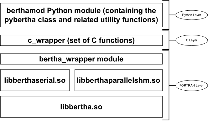
Figure 1: An overview of the BERTHA software’s layers.

In Figure 1 we outline the fundamental structure of BERTHA. All the basic kernel functions written in FORTRAN are now collected in a single Shared Object (SO) (i.e, libertha.so). Alongside there are two other SO libraries: libberthaserial.so capable of performing both the serial and parallel OpenMP based ¹⁰⁰ runs, and libberthaparalleshm.so containing all the functions needed to perform MPI ¹⁰¹ based parallel computations where also the memory burden is distributed among the processes.

We also implemented a FORTRAN module, named bertha_wrapper, containing a class implementing all the methods needed to access to all the basic quantities, such as: energy, density, DKS and overlap matrices and other. The same FORTRAN module (i.e., bertha_wrapper) is used to perform all the basic operations such as: bertha_init to perform all the memory allocations, bertha_main to run the main SCF iterations, and bertha_finalize to free all the allocated memory, and more. Finally the main PyBERTHA ⁶⁷ module has been developed using the ctypes Python module. This module provides the C-compatible data types, and allows calling functions collected in shared libraries. In order to simplify the direct interlanguage communication between Python and FORTRAN, we implemented a simple C layer called c_wrapper, also summarized in Figure 1. This Python API to BERTHA has been described in detail in Refs.74, 76 and in the present work has been further extended with new methods which allow us to extract all those quantities necessary for the DKS-in-DFT FDE implementation (e.g., the method bertha_get_density_on_grid() used to extract the values of the fitted electron density on a grid). All the new methods have been efficiently parallelized using OpenMP ¹⁰⁰. All details and computational efficiency will be given in the next sections.

3.1 The PyBerthaEmbed DKS-in-DFT FDE implementation

In this section we outline the computational strategy we adopted to implement the DKS-in-DFT FDE scheme. The developed Python program pyberthaemb.py and the related module (pyembmod) are freely available under GPLv3 license at Ref. 102. A data set collection of computational results including numerical data, parameters and job input instructions used to obtain the results of Section 4, is available and can be freely accessed at the Zenodo repository, see Ref.  103.

3.1.1 Implementation strategy

1:  import berthamod

2:  import pyembmod

3:  …

4:  bertha = berthamod.pybertha(pberthaopt.wrapperso)

5:  # set options for the DKS calculation

6:  bertha.set_fnameinput(fnameinput)

7:  bertha.set_fittfname(fittfname)

8:  …

9:  bertha.init()

10:  ovapm, eigem, fockm, eigen = bertha.run()

11:  …

12:  activefname = pberthaopt.activefile

13:  envirofname = pberthaopt.envirofile

14:  embfactory = pyembmod.pyemb(activefname,envirofname,’adf’) #jobtype=’adf’ is default

15:  embfactory.set_options(param=pberthaopt.param,….) # several paramenters to be specified in input- e.g AUG/ADZP for ADF

16:  # embfactory.set_grid_filename(pberthaopt.gridfname) # a general grid may be used

17:  …

18:  embfactory.initialize()

19:  grid = embfactory.get_grid()

20:  …

21:  rho = bertha.get_density_on_grid(grid)

22:  density=numpy.zeros((rho.shape[0],10))

23:  density[:,0] = rho

24:  …

25:  pot = embfactory.get_potential(density)

26:  …

27:  for out_iter in range (maxiter): # split-SCF scheme iterations, see text

28:   bertha.init()

29:   …

30:   bertha.set_embpot_on_grid(grid, pot)

31:   ovapm, eigem, fockm, eigen = bertha.run(eigem)

32:   rho = bertha.get_density_on_grid(grid)

33:   density=numpy.zeros((rho.shape[0],10))

34:   density[:,0] = rho

35:   pot_old=pot

36:   pot = embfactory.get_potential(density)

37:   norm_pot = numpy.sqrt(numpy.sum((pot-pot_old)**2))

38:   norm_D = numpy.linalg.norm(diffD,’fro’)

39:   norm_D = numpy.linalg.norm(diffD,’fro’)

40:   if (norm_D<(1.0e-6) and norm_pot <(1.0e-4)):

41:   bertha.finalize()

42:   break

Algorithm 1 Illustrative Python code to compute active system DKS density (using the pyberthaemb.py code), environment density and Coulomb potential (using the ADF code) and non-additive embedding potential via the pyemb module

The newly developed code is composed of two main modules: the pyembmod one, that allows to manage all the important quantities for the FDE implementation, and the pyberthamod module ⁶⁷.

Specifically, the pyemb class inside the pyembmod module allows to well isolate all the FDE data and operations increasing the level of abstraction. The module is used to manage all the required quantities for the generation of the embedding potential, that is ${v}_{\mathrm{emb}}[\tilde{\rho_{I}},\rho_{II}(\bm{r})]$. It has been engineered in a such manner that all details of the FDE low-lying implementation will be completely transparent from the PyBERTHA side. This has the advantage that all future developments and/or integration of the FDE scheme (g.e. using DKS theory also for the environment DKS-in-DKS FDE) will not affect the PyBERTHAembed code, i.e. it will remain completely unchanged. In particular in this first version the pyembmod module can handle the basic procedures previously implemented in the Psi4-rt-PyEmbed software which are based on the use of PyADF^{30, 68}, PyEmbed module^{69, 70}, and the XCFun library^{71, 72} to evaluate non-additive exchange-correlation and kinetic energy contributions on a user-defined integration grids. This approach gave us both the advantage of the code re-usability and, even more importantly, a DFT-in-DFT FDE reference implementation in which we can have the precise control over all those details and parameters from which a FDE scheme depends on (i.e., algorithms, numerical grid definition, quantum chemistry packages used to determine electronic density and Coulomb potential of the environment, basis sets, exchange-correlation functionals, etc…). This has clearly made the debugging phase in the development of PyBERTHAembed software straightforward.

Algorithm 1 reports the most important part of the pyberthaemb.py code, and it well illustrates how we can gain a relatively simple work-flow to implement FDE using the DKS level of theory for the active system using PyBERTHA and the new pyemb class for the environmental system. The pybertha class is instantiated (line 4) with the shared object bertha_wrapper.so specified as an input. The SO contains the cited c_wrapper and bertha_wrapper code which are based on the core FORTRAN libraries, namely: libbertha.so and libberthaserial.so (see Figure 1 above). After the initialization, the full DKS calculation is worked out (line 10) using the bertha.run() method. At line 14 the pyemb class is also instantiated specifying the files (specified in xyz format) for the geometries of both the active and embedding systems. The quantum chemistry software employed for the actual calculation of the environment system is specified at this stage (in the current example, and throughout this work, we used the ADF package⁵³).

All the details for the computation of the embedding system are set at line 15. This includes: the selection of the type of basis set functions, Hamiltonian, exchange-correlation functional and also the non-additive kinetic functional used to define the embedding potential. At this stage all the basis sets and exchange-correlation functionals available in the ADF library can be used. Similarly, the numerical integration grid used for the numerical representation of the embedding potential is set, both the type (global grid or active system) and the quality. By default the numerical grids internally defined by the ADF program are used, however other options are available, including the possibility to use an user-defined grid (see for instance line 16, commented).

The embfactory.initialize() method performs a stand-alone single point calculation on the embedding system. The method evaluates the nuclear and Coulomb potentials of the environment (see Eq.6) and its ground state electron density ($\rho_{II}$). All these quantities are mapped on the numerical grid. At this time, the numerical grid defined within PyADF is made available (as a numpy.array) using the get_grid() method (line 19) and used as an input for the get_density_on_grid() method of the pybertha class. This method allows to define the ground state density $\tilde{\rho}_{I}$ of the active system at DKS level of theory. $\tilde{\rho}_{I}$ is also available as a numpy.array that, after a reshape (line 22), can be used as an input of the get_potential() method of the pyemb class (line 25) to obtain the final embedding potential.

After this initial setup, we proceed to the actual FDE calculation. In this example, the embedding potential will be generated using the active subsystem density (loop structure, lines 27 to 40), using the split-SCF scheme ¹⁰⁴. Thus, in each of the spin-SCF iterations, the new set_embpot_on_grid() method of pybertha class makes both the numerical grid and the embedding potential available at the FORTRAN layer. Thus, the numerical integration of the $v^{emb}({r})$ on the fitting basis functions (Eq.24) and linear system solution (Eq.23) are efficiently evaluated in FORTRAN. The DKS matrix employed in the intervening BERTHA calculation (bertha.run(), line 31) is updated using the G-spinor representation of the embedding potential, and here the split-SCF scheme is interesting as it does not require the evaluation of the embedding potential at each SCF step taking place on the BERTHA side. The new fitted density (line 32) is used to compute a new embedding potential (line 36) which is used in for the next iteration of the split-SCF procedure ¹⁰⁴. This scheme is iterated till a convergence criteria is satisfied (line 40).

In Figure 2 we present the workflow which emphasizes the interoperability between different tasks and modules or programs involved including the layers where the actual computations are carried out. This schematic picture highlights also how the key quantities, required to implement the DKS-in-DFT FDE scheme, have different representations along the computation. As example, we focus on the electron density of the active system, $\tilde{\rho}_{I}(r)$. This quantity is evaluated at the DKS level of theory activated by the bertha.run() method within the PyBERTHAembed program. The actual calculation is done within the FORTRAN layer. At this level, $\tilde{\rho}_{I}(r)$ is represented in terms of the expansion coefficients of auxiliary fitting functions ($\bm{d}$, see Eq.19) and is stored as a FORTRAN array (of dimension $N_{aux}$). However, this representation is not useful itself for the evaluation of the embedding potential. Indeed, its evaluation and in particular the non-additive contribution requires that $\tilde{\rho}_{I}(r)$ is represented on a grid. Thus, within pyberthaemb.py, the numerical grid (GRID) evaluated within PyADF (see panel init) is made available as numpy.array and via the bertha.get_density_on_grid() method is made accessible to the FORTRAN layer (bertha_wrapper module), and stored as a FORTRAN array of dimension $npoints$. The calculation of the numerical representation of $\tilde{\rho}_{I}(r)$ on the grid is done efficiently in FORTRAN (see in Figure 2, panel a) and the latter is accessible within pyberthaemb.py as a numpy.array. Analogously, different representations are used also for the embedding potential along the workflow. Note that all quantities accessible from pyberthaemb.py, namely $\tilde{\rho}_{I}(r)$, $v^{emb}({r}_{k})$ and GRID (labelling the arrows in figure), are defined as numpy.array that can be easily manipulated within a Python source code. The computational steps which involve BERTHA are instead implemented in FORTRAN (panel a) and panel c) in Figure) and have been efficiently parallelized using OpenMP.

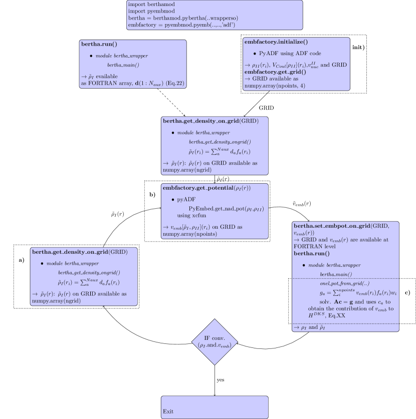
Figure 2: Working flowchart of the Pyberthaemb. In the out-of-loop section the density and electrostatic potential of the environment are obtained as grid functions (init). a) numerical representation of $\tilde{\rho}(r)$ on the grid b) PyEmbed classes are used to calculate the embedding potential. c) projection of the embedding potential onto fitting basis functions.

4 Results and Discussion

In the present section we report a series of numerical results mainly devoted to assess the correctness of our new implementation of DKS-in-DFT FDE scheme. In addition we are also reporting the computational cost and scalability with respect to the size of both the active and the embedding system. Finally, we will present an application to a series of Heavy (Rn) and Super-Heavy elements (Cn, Fl, Og) confined into a C₆₀ cage.

4.1 Initial validation and numerical stability: H₂O-NH₃

As already mentioned, in this first version of the pyembmod module we include the basic procedures previously implemented in the Psi4-rt-PyEmbed code which are based on the use of PyADF^{30, 68} and of the PyEmbed module^{69, 105}.

This poses us in an ideal framework of having a reference non relativistic DFT-in-DFT FDE implementation where we can have the precise control over all those details, and parameters, from which a FDE calculation depends on. Thus, for the sake of a direct comparison, we selected a simple molecular complex, namely the H₂O-NH₃ adduct, for which the relativistic effects are expected to be negligible. For this system we can safely compare directly the numerical results of the DKS-in-DFT FDE method, implemented here, with respect to those obtained using the DFT-in-DFT FDE scheme in the Psi4-rt-PyEmbed code ³¹.

In the adduct the water molecule is the active system that is bound to an ammonia molecule, which instead plays the role of the embedding environment. In the Psi4-rt-PyEmbed case we use basis sets obtained by the decontraction of the Gaussian cc-pVDZ, cc-pVTZ and aug-cc-pVDZ basis sets ^{106, 107} for the active system (these basis sets are referred as cc-pvdz-decon, cc-pvtz-decon and aug-cc-pvdz-decon, respectively). The same basis set has been used in the DKS calculation to define the large component of the G-spinor basis set. The corresponding small component was generated using restricted kinetic balance relation⁸⁸. Noteworthy, for these reference calculations, we have used an extremely large auxiliary fitting basis set (A4_spdfg) which gives an error on the Coulomb energy even below $10^{-6}$ Eh. The computational details for the definition of the environment, including parameters to define the embedding potential, are identical in both PyBERTHAembed and Psi4-rt-PyEmbed. In particular, the basis set used in PyADF for the calculation of the environment frozen density (ammonia) and the embedding potential is the AUG-TZ2P Slater-type set from the ADF library¹⁰⁸. As numerical grid we used the supermolecular Voronoi Polyhedra grid defined in ADF which is set defining an the integration parameter equal to 4 (this corresponds to a total number of 33280 grid points). The PBE ¹⁰⁹ exchange-correlation functional has been used for the active system while the BLYP ^{110, 111} exchange-correlation functional has been used for the ammonia molecule. The Thomas-Fermi and LDA functionals ^{112, 113} has been employed for the non-additive kinetic and non-additive exchange-correlation potential, respectively. The molecular structure of the adduct is reported in SI (Table S.1). The effect of the environment (ammonia) on the active system (water) have been evaluated comparing the dipole moment components and diagonal elements of the polarizability tensor ($\alpha_{xx},\alpha_{yy}$ and $\alpha_{zz}$) of the isolated (Free) respect to the embedded (Emb) water. We note here that the quoted polarizability values are not those for the supermolecular system, but only for the active subsystem.

The numerical results, reported in Table 1, show an evident quantitative agreement between the two implementations. Indeed, both the variations induced by the presence of the embedding system ($\Delta$ values) and the absolute values show a good agreement. Noteworthy, independently by the basis set used, the differences are below of 0.001 a.u. and 0.01 a.u. for the dipole moment components and for the polarizability tensor components, respectively. We mention that we also performed the calculations increasing the speed of light by 1 order of magnitude (i.e., c = 1370.36 a.u.) to approximate the non-relativistic limit and, as expected, we obtain almost indistinguishable results (see Table S.2). All the above findings make us confident that our implementation is both numerically stable and correct.

	Psi4-rt-PyEmbed				PyBERTHAembed
	Free	Emb	$\Delta$		Free	Emb	$\Delta$
	a) aug-cc-pvdz-decon
$\mu_{x}$	-0.35403	-0.49351	-0.13948		-0.35328	-0.49279	-0.13951
$\mu_{y}$	-0.62058	-0.62976	-0.00918		-0.61908	-0.62812	-0.00904
$\mu_{z}$	-0.00025	-0.00026	-0.00001		-0.00025	-0.00027	-0.00002
$|\mu|$	0.71446	0.80009	0.08563		0.71279	0.79836	0.08557
$\alpha_{xx}$	10.34	9.79	-0.55		10.36	9.80	-0.56
$\alpha_{yy}$	9.91	10.26	0.35		9.92	10.27	0.35
$\alpha_{zz}$	9.62	10.16	0.54		9.64	10.18	0.54
$\alpha_{iso}$	9.96	10.07	0.11		9.97	10.08	0.11
	b) cc-pvdz-decon
$\mu_{x}$	-0.38085	-0.50083	-0.11998		-0.37992	-0.50006	-0.12014
$\mu_{y}$	-0.67072	-0.67187	-0.00115		-0.66911	-0.67023	-0.00112
$\mu_{z}$	-0.00027	-0.00031	-0.00004		-0.00027	-0.00031	-0.00004
$|\mu|$	0.77130	0.83800	0.06670		0.76944	0.83622	0.06678
$\alpha_{xx}$	7.35	6.79	-0.56		7.36	6.80	-0.56
$\alpha_{yy}$	6.27	6.38	0.11		6.28	6.39	0.11
$\alpha_{zz}$	3.70	3.71	0.01		3.70	3.71	0.01
$\alpha_{iso}$	5.77	5.63	-0.14		5.78	5.63	-0.15
	c) cc-pvtz-decon
$\mu_{x}$	-0.36464	-0.49344	-0.12880		-0.36377	-0.49267	-0.12890
$\mu_{y}$	-0.64037	-0.64583	-0.00546		-0.63883	-0.64430	-0.00547
$\mu_{z}$	-0.00025	-0.00028	-0.00003		-0.00026	-0.00028	-0.00002
$|\mu|$	0.73691	0.81276	0.07585		0.73514	0.81108	0.07593
$\alpha_{xx}$	8.52	7.95	-0.57		8.53	7.96	-0.57
$\alpha_{yy}$	7.80	7.94	0.14		7.81	7.95	0.14
$\alpha_{zz}$	5.77	5.80	0.03		5.78	5.82	0.04
$\alpha_{iso}$	7.36	7.23	-0.13		7.37	7.24	-0.13

Table 1: Dipole moment (components $\mu_{x}$, $\mu_{y}$, $\mu_{z}$ and module $|\mu|$) and dipole polarizability (tensor diagonal components $\alpha_{xx}$, $\alpha_{yy}$, $\alpha_{zz}$ and isotropic contribution $\alpha_{iso}$) of both the isolated (Free) and embedded (Emb) water molecule. In the embedded water molecule, an ammonia molecule is used as environment. Data have been obtained using our new PyBERTHAembed implementation and the reference Psi4-rt-PyEmbed implementation (see text for details). The shift $\Delta$ is also reported. All numerical data are reported in atomic units (a.u.). The diagonal components of the dipole polarizability tensor have been calculated using a finite field approach using an external electric of 0.001 a.u.

	A2s	A2sp	A2spd	A2spdfg	A3spdfg	A4spdfg
Naux	(19)	(67)	(163)	(338)	(403)	(544)
$\mu_{x}$	-0.49845	-0.50555	-0.49264	-0.49250	-0.49261	-0.49267
$\mu_{y}$	-0.65654	-0.64784	-0.64804	-0.64415	-0.64445	-0.64429
$\mu_{z}$	-0.00034	-0.00051	-0.00024	-0.00028	-0.00028	-0.00028
$|\mu|$	0.824322	0.82175	0.81404	0.81086	0.81116	0.81107
$\alpha_{xx}$	8.46	7.95	7.96	7.96	7.96	7.96
$\alpha_{yy}$	7.19	8.12	7.95	7.95	7.95	7.95
$\alpha_{zz}$	3.90	6.08	5.80	5.81	5.81	5.82
$\alpha_{so}$	6.52	7.38	7.24	7.24	7.24	7.24
$\Delta{E}_{J}$	1.51(10-2)	4.47(10-3)	2.8(10-4)	4.8(10-6)	1.9(10-6)	5.0(10-7)

Table 2: Dipole moment (components $\mu_{x}$, $\mu_{y}$, $\mu_{z}$ and module $|\mu|$) and dipole polarizability (tensor diagonal components $\alpha_{xx}$, $\alpha_{yy}$, $\alpha_{zz}$ and isotropic contribution $\alpha_{iso}$) of the embedded water molecule (water-ammonia system). Data have been obtained with our new PyBERTHAembed implementation (using a G-spinor basis functions derived from the cc-pvtz-decon basis) and several auxiliary density fitting basis sets (A2_s, A2_sp, A2_spd, A2_spdfg, A3_spdfg and A4_spdfg). The size of different fitting basis sets (N_aux) are reported in parenthesis. $\Delta{E}_{J}$ is the absolute error on the Coulomb energy due to the density fitting. The diagonal components of the dipole polarizability tensor have been calculated using a finite field approach using an external electric of 0.001. All numerical data are reported in atomic units (a.u.). See text for the fitting basis set definition and further details.

As we have extensively described in the previous section, our implementation strongly benefits of the use of auxiliary fitting functions, both in the definition of the embedding potential and as intermediate quantities to obtain the G-spinor matrix representation of the embedding potential. Thus, it appears mandatory to investigate the impact of the quality of the density fitting basis set on the final results of DKS-in-DFT FDE calculations. In addition to the limit auxiliary fitting basis set employed above we generated five fitting basis sets (A2_s, A2_sp, A2_spd, A2_spdfg and A3_spdfg) of increasing accuracy. We have adopted a procedure which is strictly related with that proposed by Köster et al. and employed in Demon2K code (see appendix of Ref.114). All the fitting basis sets are explicitly reported in SI, while the results are reported in Table 2. In the Table we also show the absolute error in the Coulomb energy ($\Delta{E}_{J}$), which is the quantity that is variationally optimized in the fitting procedure and typically regarded as its quality index. This numerical test shows that the use of density fitting does not introduce any significant instability in the DKS calculation of the active system, also in presence of the embedding potential. The $\Delta{E}_{J}$ values are showing a convergent trend of both the dipole moment components and the polarizability when the quality of the fitting basis set is increased. The fitting basis sets A2_s+ and A2_sp+, bearing only s- and p-type Hermite Gaussian functions, have values of $\Delta{E}_{J}$ larger than 1 mEh and are clearly inadequate to reproduce the reference results. Very accurate results can already be obtained starting from the A2_spd auxiliary basis set (i.e., 163 functions for the water molecule). It is interesting to note that the $\Delta{E}_{J}$ associated with this basis set is of the same order of magnitude of that typically required (0.1 mEh per atom) in standard calculations based on density fitting without including FDE. Thus, these preliminary results suggest that the variational density fitting scheme can safely be applied in the implementation of DKS-in-DFT method without jeopardizing its accuracy.

4.2 Computational efficiency : gold clusters in water

It is interesting now to put forward some assessments on the computational efficiency of our DKS-in-DFT FDE implementation, together with its scaling properties in terms of time statistics and memory usage. This analysis will give us a detailed overview of the the computational burden, and possible bottlenecks, along the relatively complex workflow we implemented (using different quantum chemistry packages and programming languages). Furthermore, it will be a solid starting point for future optimizations and developments (e.g. DKS-in-DKS or coupled real time DKS-in-DKS). As a test case we have chosen a series of gold clusters (Au₂, Au₄, Au₈) embedded using an increasing number (5, 10, 20, 40 and 80) of water molecules. In all cases, for Au the large component of the G-spinor basis set was generated by uncontracting double-$\zeta$ quality Dyall’s basis sets  ^{115, 116, 117} augmented with the related polarization and correlating functions ($24s19p12d9f1g$), while the corresponding small component basis was generated using the restricted kinetic balance relation. For the water molecules of the environment we used the DZ Slater-type set from the ADF library¹⁰⁸. The supermolecular grid defined in PyADF, corresponding to an integration parameter of 4 in the ADF package, has been used. The BLYP ^{110, 111} exchange-correlation functional is used for the ground state calculation of the embedding system, while the Thomas-Fermi and LDA functionals ^{112, 113} have been employed for the non-additive kinetic and non-additive exchange-correlation potential, respectively. The molecular structure of all the adducts are available in Ref.103. All the calculations have been performed on a Dual Intel(R) Xeon(R) CPU E5-2684 v4 running at 2.10GHz, equipped with 251 GiB of RAM. We used the Intel Parallel Studio XE 2018 ¹¹⁸ to compile the FORTRAN code and Python 3.8.5 (from Anaconda, Inc.) and NumPy version 1.19.2 for the Python code. We used PyADF^{30, 68} as recently ported to Python3⁶⁵, ADF(version 2019.307) for the core DFT calculations of the environment and XCFun library (version 1.99).^{71, 72, 119}

The results are reported in Table 3 and in Table 4, where, together with the total elapsed time (t^d) for each SCF iteration including the FDE contribution, we also partition between different tasks related with the FDE implementation, namely: a) numerical representation of active system fitted density on grid, $\tilde{\rho}(r)$; b) calculation of the non-additive terms of embedding potential by PyADF (with the PyEmbed class); c) projection of the embedding potential onto fitting basis functions. In the Tables we also report the maximum memory usage for the SCF procedure ("Mem"), the number of points of grid and the timing for the "init" phase which involves: the evaluation of the ground state electronic density of the environmental together with the associated Coulomb potential, and their mapping on the numerical grid. We recall that the electron density of the environment is kept frozen, thus this initial step is done once at the beginning of the procedure. All tasks are also highlighted (using the same labeling: a, b, c and init) in Figure 2.

As general remark we may state that the FDE contribution to the total time is relatively small. By increasing the size of the active system (Au₂, Au₄ and Au₈), and keeping fixed the environment (using ten water molecules), see Table 3, the relative impact of the FDE computational phase decreases. It passes from 13.3% for Au₂(H₂O)₁₀ to 0.9% for Au₈(H₂O)₁₀. This may be expected since tasks a), b) and c) have a more favorable scaling than the DKS calculation (i.e., $O(N^{3})$). The computational cost for the step a) and c) is proportional to the product $N^{aux}\cdot N_{gridpoints}$, where: $N^{aux}$ is the total number of the auxiliary fitting functions in the active system, and $N_{gridpoints}$ total number of grid points. Thus, the computational cost should scale as $O(N^{2})$ (being $N$ the dimension of the active system). The actual scaling is much lower (i.e., slightly higher than $O(N)$) mainly because the total grid points are largely dominated by the environmental system (see number of grid points, $N_{gridpoints}$, as reported in Table 3 ). Concerning the step b) and considering the fact that the environment is maintained fixed, it scales, as expected, linearly with number of points of the grid, $N_{gridpoints}$. The maximum use of memory, during the whole DKS-in-DFT FDE procedure, increases with respect to the number of Au atoms being N^1.7, which is close to the theoretical value N².

When we fix the active system (Au₄) increasing instead the size of the environment, see Table 4, the relative computational cost to include the embedding passes from 2.2%, in the case of Au₄@(H₂O)₅, to 16.1% for Au₄@(H₂O)₈₀. In this case, all tasks associated with the FDE procedure (a,b, and c) have a computational burden which increases linearly with the size of the environment (and the number of total grid points, see Figure S1 in SI), while the maximum memory usage during the SCF procedure is almost independent from the number of water molecules in environment, as only a slight increase can be observed.

Table 3: Elapsed real time (s). ^a: fitted density on grid; ^b : calculation of the non-additive terms of embedding potential by PyADF (with PyEmbed classes); ^c : projection of the embedding potential onto fitting basis functions ^d : Total time for a single DKS self-consistent field interaction. All the calculations have been performed in a Dual Intel(R) Xeon(R) CPU E5-2684 v4 running at 2.10GHz, equipped with 251 GiB of RAM. We used the Intel Parallel Studio XE 2018 ¹¹⁸ to compile the FORTRAN code and instead Python 3.8.5 Anaconda. Inc and NumPy version 1.19.2 for the Python code. See text for further details.

System	ta	tb	tc	td	Mem(MB)	grid points	init embfactory
Au2(H2O)10	1.47	2.74	1.48	42.68	1165	213248	138.9 (8.8)
Au4(H2O)10	3.06	2.84	3.09	260.16	2164	221824	127.9 (9.0)
Au8(H2O)10	6.62	3.05	6.70	1849.90	7572	237824	154.7 (9.8)

Table 4: Elapsed real time (s). ^a: fitted density on grid; ^b : calculation of the non-additive terms of embedding potential by PyADF (with PyEmbed classes); ^c : projection of the embedding potential onto fitting basis functions ^d : Total time for a single DKS self-consistent field interaction. All the calculations have been performed in a Dual Intel(R) Xeon(R) CPU E5-2684 v4 running at 2.10GHz, equipped with 251 GiB of RAM. We used the Intel Parallel Studio XE 2018 ¹¹⁸ to compile the FORTRAN code and instead Python 3.8.5 Anaconda. Inc and NumPy version 1.19.2 for the Python code. See text for further details.

System	ta	tb	tc	td	Mem(Mb)	grid points	init embfactory
Au4(H2O)5	1.97	1.84	1.99	257.70	2137	143232	102.3 (5.9)
Au4(H2O)10	3.06	2.84	3.09	260.16	2164	221824	127.9 (9.0)
Au4(H2O)20	5.04	4.71	5.07	260.44	2225	366336	215.4 (14.8)
Au4(H2O)40	8.69	8.09	8.71	270.19	2331	630144	641.0 (25.8)
Au4(H2O)80	16.27	15.19	16.40	295.65	2354	1184896	2600.1 (47.8)

As already mentioned in the previous sections we have recently developed an OpenMP parallel version of BERTHA which can be easily used directly via the Python API ⁷⁵. This only requires the berthamod module, which refers to the shared object libberthaserial.so, to be compiled with OpenMP flag set. Thus, here we have extended the OpenMP parallelization to those steps of the FDE procedure in which the BERTHA code is directly involved, namely the steps a) and c), see above. The results are given for the Au₄(H₂O)₈₀ system and are reported in Table 5. These steps have been efficiently parallelized and we are able to achieve a speed-up of 31.1 and 29.8 using 32 threads, respectively for step a and d. Noteworthy, for this parallel implementation the FDE phase is about 45% of the total elapsed time and is dominated by the computation task that remains serial part. Indeed, using 32 threads the task b takes 15.20 sec of the total 35.8 sec necessary for each SCF iteration. This task, that is related to the generation of the non-additive kinetic and exchange-correlation on grid is currently carried out by the PyEmbed component in PyADF. Regarding the memory usage, in our OpenMP implementation we observe a linear growth of memory usage with respect to the number of the employed threads. This is somehow expected due to the obvious data replication in the OpenMP implementation. Despite one may expect that there may be room for a further optimization, we note that even in the current version the implementation is not memory-bound. In the case of 32 threads we found a maximum memory usage of about 11 GiB which demonstrates that such kind of calculations, and even larger ones, can be routinely carried out on the current multi-core architectures which may easily achieve 64 to 128 cores and 512 to 1024 GiB per node.

Table 5: Elapsed real time (s) for the Au₄(H₂O)₈₀ system. ^a: fitted density on grid; ^b : calculation of the non-additive terms of embedding potential by PyADF (with PyEmbed classes); ^c : projection of the embedding potential onto fitting basis functions ^d : Total time for a single DKS self-consistent field interaction. All the calculations have been performed in a Dual Intel(R) Xeon(R) CPU E5-2684 v4 running at 2.10GHz, equipped with 251 GiB of RAM and all the running time have been obtained using the dynamic schedule in OpenMP. We used the Intel Parallel Studio XE 2018 ¹¹⁸ to compile the FORTRAN code and instead Python 3.8.5 Anaconda. Inc and NumPy version 1.19.2 for the Python code. See text for further details.

n. threads	ta	tb	tc	td	Mem(Mb)	init embfactory
1	16.16	15.16	16.40	291.06	2343	2634.4 (48.5)
2	8.12	15.23	8.30	158.20	2638	2633.1 (48.8)
4	4.07	15.23	4.11	91.10	3210	2631.4 (48.5)
8	2.03	15.32	2.06	60.48	4377	2655.7 (48.4)
16	1.04	15.23	1.10	43.67	6632	2603.4 (48.5)
32	0.52	15.20	0.55	35.80	11020	2601.4 (49.1)

4.3 The generation of atom-endohedral fullerenes model potentials

We conclude our work by showcasing how we can leverage our FDE implementation to determine fullerene-atom model potentials, that are applicable for species across the periodic table.

Over the past decades, it has been recognized that fullerenes can serve as containers for other, smaller species¹²⁰. As such, there has been considerable interest in understanding how such smaller species behave under confinement, both from a fundamental point of view as well as due to possible technological applications we mention: the potential use as seed materials in solid state quantum computation ¹²¹, and the use as agents for improving the super-conducting ability of materials ¹²².

From a more fundamental perspective, the study of how atomic species behave under such confinement is a particularly active domain. With respect to the use of theoretical approaches, a number of studies have been reported that employed, in most cases, simple models of the C₆₀ cage potential to represent the confinement potential ^{123, 124, 125}. A model where only electrons of the guest atoms are considered while the $C_{60}$ cage is modelled, in most cases, by a short-range attractive $V_{c}(r)$ spherical potential defined as follows:

$$V_{c}(r)=\left\{\begin{matrix}U_{0},&if\ \ r_{0}\leq r\leq r_{0}+\Delta\\ 0,&otherwise\end{matrix}\right.$$ (26)

where $r_{0}=5.8\ a.u.$ and $U_{0}=-0.30134\ a.u.$ and $\Delta=1.9\ a.u$ represent the finite thickness of the spherical potential¹²³. Other model potentials have been proposed ¹²⁶, as well as other approaches to avoid numerical instability related to the sharp form of those potentials ^{127, 128}. An alternative approach may be to start from the embedding potential generated in the FDE scheme, which is expected to be highly accurate and without artificial discontinuities. In the following, we propose a possibly general procedure to build model potentials for atomic calculations and, with this aim, we compare the results, in terms of HOMO-LUMO gap, for a set of heavy atoms, obtained using the Frozen Density Embedding (FDE) procedure respect to the simple spherical potential (SPM) modelled by Eq. 26. Practically we applied the FDE scheme to a set of neutral endohedral fullerenes A@C₆₀ (A=Rn,Og,Fl,Cn), where the atom A (i.e., active system) is embedded in a fullerene (i.e., environment) and always placed at the exact center of the C₆₀. Finally, by comparing the embedding potential (EMBP) and its spherical average with respect to the cited spherical potential model (SPM), we propose a simple numerical recipe that can be used within the FDE scheme to possibly extract more accurate potentials to be tested in atomic calculations.

Before proceeding in the comparison of different models, we have compared for the Rn atom the ability of FDE to capture environment effects on orbital energies, with respect to standard (supramolecular) DFT calculations. Our results, shown in Figure S2 in the supplementary information, show that there is a good agreement between the FDE and supramolecular calculations, with FDE yielding overall slightly larger orbital energy shifts, that are nevertheless very homogeneous across the different orbitals. From these results we conclude that FDE is, in effect, capable of correctly describing the fullerene cage’s effect onto the atom’s electronic structure.

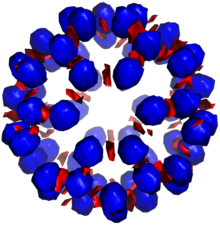
Figure 3: The embedding potential (EMBP) in blue (negative) and red (positive), computed for the Rn@C₆₀ system. We report the contour plot at $\pm 0.3$ a.u. It is important to underlined as the plotted values are the result of a Nearest-neighbor interpolation performed starting from the original non homogeneous ADF grid.

All calculations, reported in the following, were carried out using a basis set for the active system (i.e., A=Rn,Og,Fl,Cn) generated by uncontracting triple–$\zeta$ quality Dyall’s basis sets ^{129, 117, 116, 130} augmented with the related polarization and correlating functions. Final basis set schemes are as follows: Cn (32s29p20d14f7g2h), Rn (31s27p18d12f4g1h), Fl and Og (31s30p21d14f6g2h).

For all the elements we used auxiliary basis sets already employed in Ref.131 and are explicitly reported in SI. While for the environment (i.e., the C₆₀), computed using the ADF code, we use the TZP basis set. In both cases we use the BLYP ^{110, 111} exchange-correlation functional, while for the nonadditive kinetic and nonadditive exchange-correlation terms in the generation of the embedding potential, the Thomas-Fermi and LDA functionals are used, respectively.

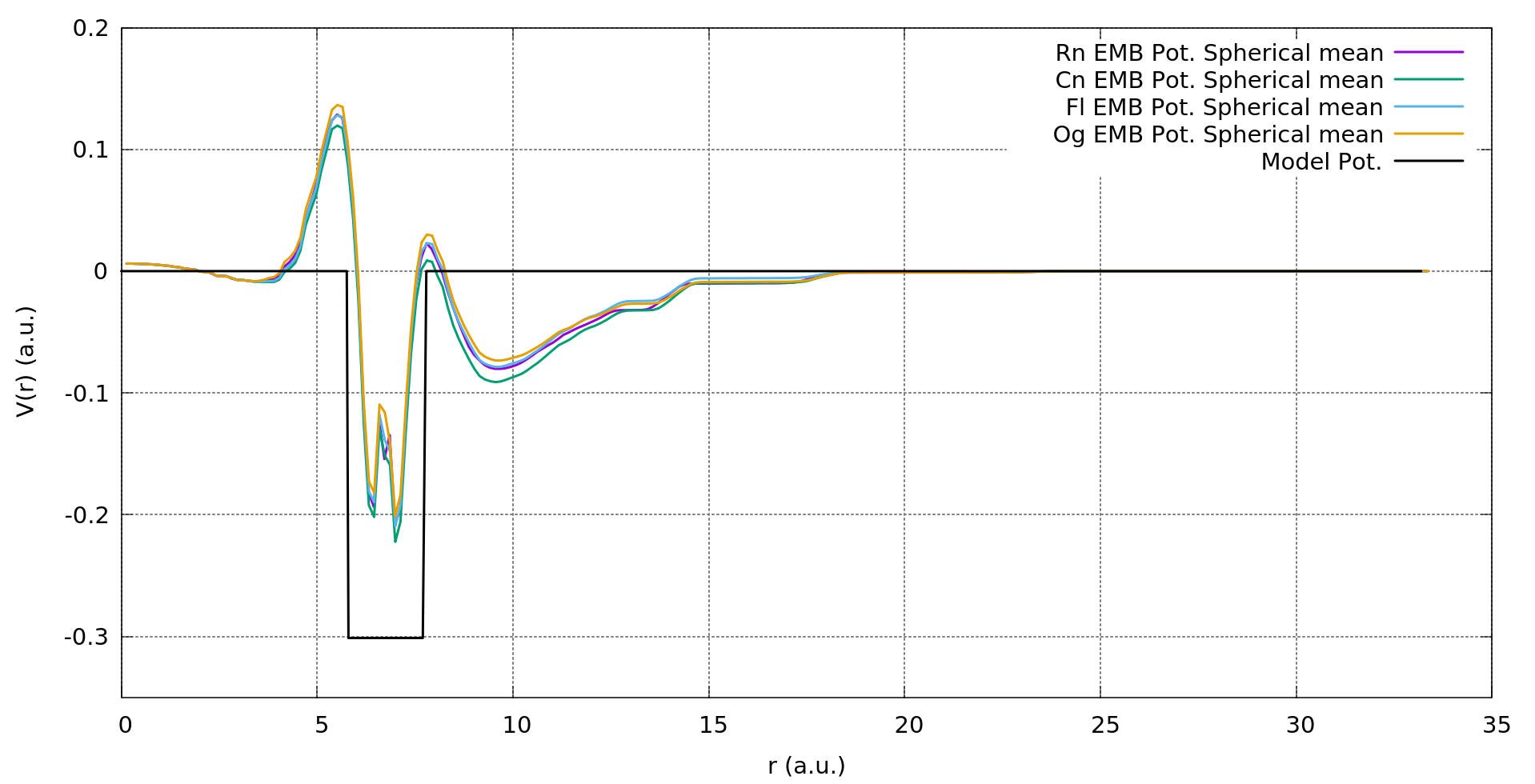
Figure 4: The spherical average of the Rn, Og, Cn and Fl embedding potential together with the simple short-range attractive spherical potential as reported in Eq. 26.

Figure 3 reports the EMBP of the Rn@C₆₀ system. The EMBP shows positive values centered at nuclei positions, and negative values located in correspondence of the bonds. As one may expect the EMBP potential, while maintaining an overall spherical shape, is clearly different with respect to a simple short-range attractive $V_{c}(r)$ spherical potential. Indeed, if we consider the spherical average of the EMBP (see SI for details on the spherical average procedure employed) extracted for the various A@C₆₀ systems, as reported in Figure 4, while the EMBP seems to detect the same short-range attractive values surely it shows a more complex radial structure. The spherical average of the EMBP shows a positive repulsive value immediately before the inner C₆₀ surface and, maybe more importantly, never completely goes to zero, not even at the center of the fullerene where the atom A is placed.

Atom	SPM	FDE C60	EMBP	Rn based EMBP
			Spherical Average	Spherical Average
Rn	0.118680	0.209643	0.207990	…
Cn	0.055807	0.144685	0.144693	0.147514
Fl	0.072251	0.110471	0.110467	0.108101
Og	0.148040	0.139842	0.139300	0.134420

Table 6: HOMO-LUMO gap energies (a.u.).

Not surprisingly, the final results (see Table 6) in terms of HOMO-LUMO gap for the spherical model potential are quite different respect to the results obtained using the FDE procedure. Indeed, as we mentioned, the overall shape of the EMBP is quite different respect to a simple spherical ones, see Figure 3. Nevertheless, is interesting to note as the spherical average seems to work well. Comparing the results obtained from the full FDE procedure respect to the ones computed using a model potential that is the spherical average of the EMBP, respectively columns 3 and 4 of Table 6, one can easily note that the spherical average is able to well reproduce the electronic structures of the active system (i.e., the central atom) including HOMO-LUMO gaps values with an error that is generally less the 1%. Similar conclusions can be drawn looking at Figure 5, where we report instead all the differences in orbital energies with respect to the isolated Rn atom for all the occupied orbitals. Once again both the EMBP (i.e., the FDE procedure) and its spherical average lead to similar results. Instead using the simple spherical model the energy shift is always the opposite.

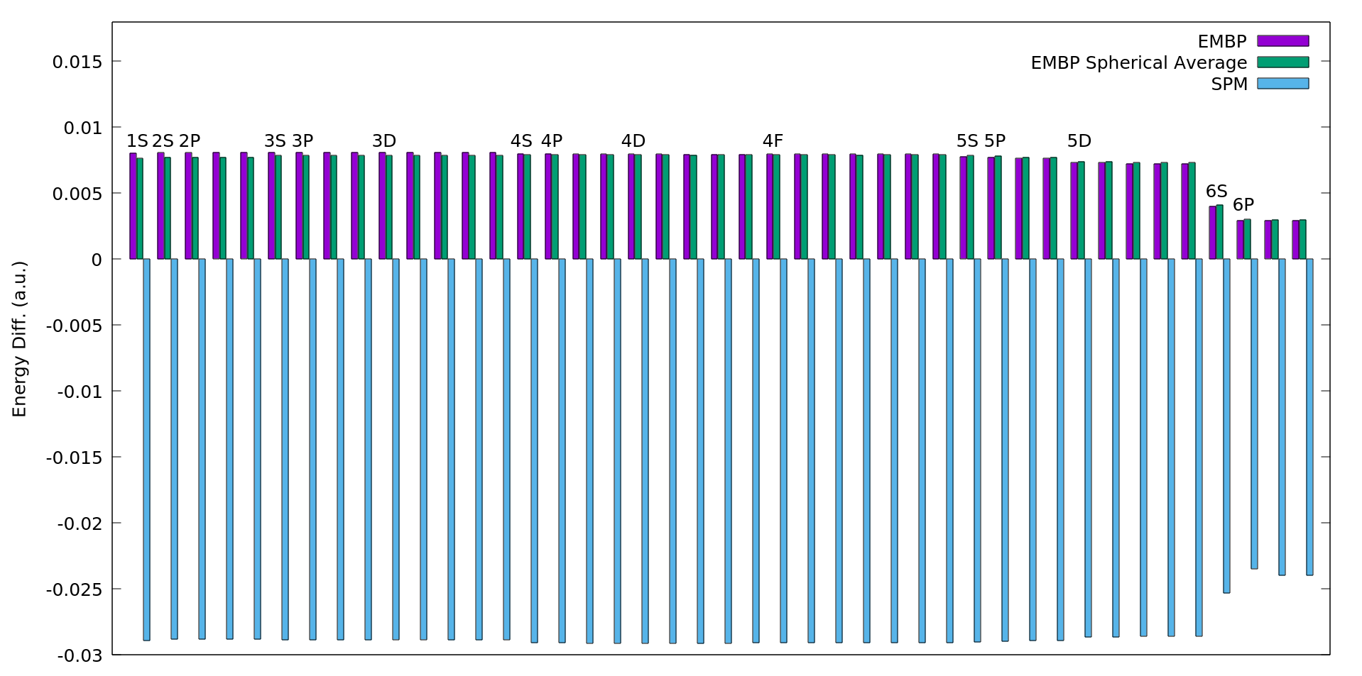
Figure 5: Differences in orbital energies with respect to the isolated Rn atom for all occupied orbitals for: the SPM model, the EMBP and the Spherical average of the EMBP.

Finally, and maybe more interestingly, if we consider column 5 of Table 6 we see that we can obtain the HOMO-LUMO gaps for all the atoms with an error that is always less then 4% using a Rn based EMBP spherical average. Thus, we computed the spherical average of the EMBP for the Rn@C₆₀ system and using this single model potential we have been able to quantitatively well reproduce the HOMO-LUMO gap for all the other A@C₆₀ systems. This latter result let us clearly envision a practical approach to be used to build model potential as a result of the FDE procedure.

5 Conclusions and perspectives

Including environmental effects based on first-principles is of paramount importance in order to obtain an accurate description of molecular species in solution and in confined spaces. Among others, the Frozen Density Embedding (FDE) density functional theory represents a embedding scheme in which environmental effects are included by considering explicitly the environmental system by means of its "frozen" electron density. In the present paper, we reported our extension of the full 4-component relativistic Dirac-Kohn-Sham method, as implemented in the BERTHA code, to include environmental and confined effects with the FDE scheme (DKS-in-DFT FDE) using the PyADF framework. We described how its complex workflow associated with its implementation can be enormously facilitated by the fact that both BERTHA (PyBERTHA) and PyADF, with their Python API, they gave us an ideal framework of development. The recent development of the Psi4-rt-Embed code³¹, which is also based on PyADF for FDE while uses Psi4Numpy code for the active system, represented an ideal reference implementation to assesses the correctness of our new DKS-in-DFT FDE implementation.

PyBERTHAembed uses the density fitting technique at the key points of the interface between PyBERTHA and PyADF. We showed that this results both in a very efficient numerical representation of the electron density of the active system and in a straightforward evaluation of the matrix representation in the relativistic G-spinor basis of the embedding potential.

The accuracy and numerical stability of this approach, also using different auxiliary fitting basis sets, has been demonstrated on the simple NH₃-H₂O system. We compared the dipole moment components and diagonal elements of the polarizability tensor of the isolated water molecule with respect to the embedded water (i.e., NH₃-H₂O system). We performed the calculations using both our DKS-in-DFT FDE implementation as well as the previously implemented Psi4-rt-PyEmbed code. The numerical results shown an evident quantitative agreement between the two implementations. Indeed, both the variations induced by the presence of the embedding system and the absolute values of both the dipole moments and polarizability show a good agreement. Noteworthy, independently by the basis set used, the differences are below of 0.001 a.u. and 0.01 a.u. for the dipole moment components and for the polarizability tensor components, respectively.

We evaluated also the computational burden on a series of gold clusters (Au_n, with $n=2,4,8$) embedded into an increasing number of water molecules (5, 10, 20, 40 and 80 water molecules). We found the our implementation approximately scales linearly both with respect to the size of the frozen surrounding environment and the size of the active system. We efficiently parallelized, using OpenMP, two of the most demanding steps on our computation, that is the computation of the numerical representation of active system fitted density on grid, as well as the projection of the embedding potential onto fitting basis functions. The results reported show that we are capable of reaching a final speedup of 31.1 and 29.8 using 32 threads for the two cited steps respectively.

Finally, we applied this new implementation to a series of Heavy (Rn) and Super-Heavy elements (Cn, Fl, Og) embedded in a C₆₀ cage to study the confinement effect induced by C₆₀ on their electronic structure. An analysis of the embedding potential demonstrated that it can be well approximated by a simple radial potential which is marginally affected by the nature of the central atom. These latter results let us clearly envision a practical approach to be used to build model potential as a results of the FDE procedure.

References

- Schwerdtfeger et al. 2020 Schwerdtfeger, P.; Smits, O. R.; Pyykkö, P. The periodic table and the physics that drives it. Nature Reviews Chemistry 2020, 4, 359–380, DOI: 10.1038/s41570-020-0195-y
- Pyykkö 2012 Pyykkö, P. Relativistic effects in chemistry: more common than you thought. Annu. Rev. Phys. Chem. 2012, 63, 45–64, DOI: 10.1146/annurev-physchem-032511-143755
- Türler and Pershina 2013 Türler, A.; Pershina, V. Advances in the Production and Chemistry of the Heaviest Elements. Chem. Rev. 2013, 113, 1237–1312, DOI: 10.1021/cr3002438
- Giuliani et al. 2019 Giuliani, S. A.; Matheson, Z.; Nazarewicz, W.; Olsen, E.; Reinhard, P. G.; Sadhukhan, J.; Schuetrumpf, B.; Schunck, N.; Schwerdtfeger, P. Colloquium: Superheavy elements: Oganesson and beyond. Rev. Mod. Phys. 2019, 91, 011001, DOI: 10.1103/RevModPhys.91.011001
- Orozco and Luque 2000 Orozco, M.; Luque, F. J. Theoretical Methods for the Description of the Solvent Effect in Biomolecular Systems. Chem. Rev. 2000, 100, 4187–4226, DOI: 10.1021/cr990052a
- Maher et al. 2012 Maher, K.; Bargar, J. R.; Brown, G. E. Environmental Speciation of Actinides. Inorg. Chem. 2012, 52, 3510–3532, DOI: 10.1021/ic301686d
- Kumpulainen et al. 2016 Kumpulainen, T.; Lang, B.; Rosspeintner, A.; Vauthey, E. Ultrafast Elementary Photochemical Processes of Organic Molecules in Liquid Solution. Chem. Rev. 2016, 117, 10826–10939, DOI: 10.1021/acs.chemrev.6b00491
- Gerber et al. 2020 Gerber, E.; Romanchuk, A. Y.; Pidchenko, I.; Amidani, L.; Rossberg, A.; Hennig, C.; Vaughan, G. B. M.; Trigub, A.; Egorova, T.; Bauters, S.; Plakhova, T.; Hunault, M. O. J. Y.; Weiss, S.; Butorin, S. M.; Scheinost, A. C.; Kalmykov, S. N.; Kvashnina, K. O. The missing pieces of the \cePuO2 nanoparticle puzzle. Nanoscale 2020, 12, 18039–18048, DOI: 10.1039/d0nr03767b
- Dupuy et al. 2021 Dupuy, R.; Richter, C.; Winter, B.; Meijer, G.; Schlögl, R.; Bluhm, H. Core level photoelectron spectroscopy of heterogeneous reactions at liquid–vapor interfaces: Current status, challenges, and prospects. J. Chem. Phys. 2021, 154, 060901, DOI: 10.1063/5.0036178
- Warshel and Levitt 1976 Warshel, A.; Levitt, M. Theoretical studies of enzymic reactions: Dielectric, electrostatic and steric stabilization of the carbonium ion in the reaction of lysozyme. J. Mol. Biol. 1976, 103, 227–249, DOI: 10.1016/0022-2836(76)90311-9
- Tomasi et al. 2005 Tomasi, J.; Mennucci, B.; Cammi, R. Quantum Mechanical Continuum Solvation Models. Chem. Rev. 2005, 105, 2999–3094, DOI: 10.1021/cr9904009
- Huang and Carter 2008 Huang, P.; Carter, E. A. Advances in Correlated Electronic Structure Methods for Solids, Surfaces, and Nanostructures. Annu. Rev. Phys. Chem 2008, 59, 261–290, DOI: 10.1146/annurev.physchem.59.032607.093528
- Gomes and Jacob 2012 Gomes, A. S. P.; Jacob, C. R. Quantum-chemical embedding methods for treating local electronic excitations in complex chemical systems. Annu. Rep. Prog. Chem., Sect. C: Phys. Chem. 2012, 108, 222, DOI: 10.1039/c2pc90007f
- Sun and Chan 2016 Sun, Q.; Chan, G. K.-L. Quantum Embedding Theories. Acc. Chem. Res. 2016, 49, 2705–2712, DOI: 10.1021/acs.accounts.6b00356
- Jones et al. 2020 Jones, L. O.; Mosquera, M. A.; Schatz, G. C.; Ratner, M. A. Embedding Methods for Quantum Chemistry: Applications from Materials to Life Sciences. J. Am. Chem. Soc. 2020, 142, 3281–3295, DOI: 10.1021/jacs.9b10780
- Wesolowski and Warshel 1993 Wesolowski, T. A.; Warshel, A. Frozen density functional approach for ab initio calculations of solvated molecules. J. Phys. Chem. 1993, 97, 8050–8053, DOI: 10.1021/j100132a040
- Wesolowski et al. 2015 Wesolowski, T. A.; Shedge, S.; Zhou, X. Frozen-Density Embedding Strategy for Multilevel Simulations of Electronic Structure. Chem. Rev. 2015, 115, 5891–5928, DOI: 10.1021/cr500502v
- Senatore and Subbaswamy 1986 Senatore, G.; Subbaswamy, K. R. Density dependence of the dielectric constant of rare-gas crystals. Phys. Rev. B 1986, 34, 5754–5757, DOI: 10.1103/PhysRevB.34.5754
- Cortona 1992 Cortona, P. Direct determination of self-consistent total energies and charge densities of solids: A study of the cohesive properties of the alkali halides. Phys. Rev. B 1992, 46, 2008–2014, DOI: 10.1103/PhysRevB.46.2008
- Iannuzzi et al. 2006 Iannuzzi, M.; Kirchner, B.; Hutter, J. Density functional embedding for molecular systems. Chem. Phys. Lett. 2006, 421, 16–20, DOI: 10.1016/j.cplett.2005.08.155
- Jacob et al. 2008 Jacob, C. R.; Neugebauer, J.; Visscher, L. A flexible implementation of frozen-density embedding for use in multilevel simulations. J. Comput. Chem. 2008, 29, 1011–1018, DOI: 10.1002/jcc.20861
- Klüner et al. 2002 Klüner, T.; Govind, N.; Wang, Y. A.; Carter, E. A. Periodic density functional embedding theory for complete active space self-consistent field and configuration interaction calculations: Ground and excited states. J. Chem. Phys. 2002, 116, 42, DOI: 10.1063/1.1420748
- Govind et al. 1998 Govind, N.; Wang, Y.; da Silva, A.; Carter, E. Accurate ab initio energetics of extended systems via explicit correlation embedded in a density functional environment. Chem. Phys. Lett. 1998, 295, 129–134, DOI: 10.1016/s0009-2614(98)00939-7
- Huang and Carter 2006 Huang, P.; Carter, E. A. Self-consistent embedding theory for locally correlated configuration interaction wave functions in condensed matter. J. Chem. Phys 2006, 125, 084102, DOI: 10.1063/1.2336428
- Dresselhaus and Neugebauer 2015 Dresselhaus, T.; Neugebauer, J. Part and whole in wavefunction/DFT embedding. Theor. Chem. Acc. 2015, 134, DOI: 10.1007/s00214-015-1697-4
- Gomes et al. 2008 Gomes, A. S. P.; Jacob, C. R.; Visscher, L. Calculation of local excitations in large systems by embedding wave-function theory in density-functional theory. Phys. Chem. Chem. Phys. 2008, 10, 5353, DOI: 10.1039/b805739g
- Götz et al. 2014 Götz, A. W.; Autschbach, J.; Visscher, L. Calculation of nuclear spin-spin coupling constants using frozen density embedding. J. Chem. Phys. 2014, 140, 104107, DOI: 10.1063/1.4864053
- Olejniczak et al. 2017 Olejniczak, M.; Bast, R.; Gomes, A. S. P. On the calculation of second-order magnetic properties using subsystem approaches in a relativistic framework. Phys. Chem. Chem. Phys. 2017, 19, 8400–8415, DOI: 10.1039/c6cp08561j
- Halbert et al. 2020 Halbert, L.; Olejniczak, M.; Vallet, V.; Gomes, A. S. P. Investigating solvent effects on the magnetic properties of molybdate ions (MoO) with relativistic embedding. Int. J. Quantum Chem. 2020, 120, e26207, DOI: 10.1002/qua.26207
- Jacob et al. 2011 Jacob, C. R.; Beyhan, S. M.; Bulo, R. E.; Gomes, A. S. P.; Götz, A. W.; Kiewisch, K.; Sikkema, J.; Visscher, L. PyADF - A scripting framework for multiscale quantum chemistry. J. Comput. Chem. 2011, 32, 2328–2338, DOI: 10.1002/jcc.21810
- De Santis et al. 2020 De Santis, M.; Belpassi, L.; Jacob, C. R.; Severo Pereira Gomes, A.; Tarantelli, F.; Visscher, L.; Storchi, L. Environmental Effects with Frozen-Density Embedding in Real-Time Time-Dependent Density Functional Theory Using Localized Basis Functions. J. Chem. Theory Comput. 2020, 16, 5695–5711, DOI: 10.1021/acs.jctc.0c00603
- Casida and Wesolowski 2004 Casida, M. E.; Wesolowski, T. A. Generalization of the Kohn-Sham equations with constrained electron density formalism and its time-dependent response theory formulation. Int. J. Quantum Chem. 2004, 96, 577–588, DOI: 10.1002/qua.10744
- Neugebauer 2007 Neugebauer, J. Couplings between electronic transitions in a subsystem formulation of time-dependent density functional theory. J. Chem. Phys. 2007, 126, 134116, DOI: 10.1063/1.2713754
- Neugebauer 2009 Neugebauer, J. On the calculation of general response properties in subsystem density functional theory. J. Chem. Phys. 2009, 131, 084104, DOI: 10.1063/1.3212883
- Tölle et al. 2019 Tölle, J.; Böckers, M.; Neugebauer, J. Exact subsystem time-dependent density-functional theory. J. Chem. Phys. 2019, 150, 181101, DOI: 10.1063/1.5097124
- Tölle et al. 2019 Tölle, J.; Böckers, M.; Niemeyer, N.; Neugebauer, J. Inter-subsystem charge-transfer excitations in exact subsystem time-dependent density-functional theory. J. Chem. Phys. 2019, 151, 174109, DOI: 10.1063/1.5121908
- Krishtal et al. 2015 Krishtal, A.; Ceresoli, D.; Pavanello, M. Subsystem real-time time dependent density functional theory. J. Chem. Phys. 2015, 142, 154116, DOI: 10.1063/1.4918276
- Fux et al. 2010 Fux, S.; Jacob, C. R.; Neugebauer, J.; Visscher, L.; Reiher, M. Accurate frozen-density embedding potentials as a first step towards a subsystem description of covalent bonds. J. Chem. Phys. 2010, 132, 164101, DOI: 10.1063/1.3376251
- Götz et al. 2009 Götz, A. W.; Beyhan, S. M.; Visscher, L. Performance of Kinetic Energy Functionals for Interaction Energies in a Subsystem Formulation of Density Functional Theory. J. Chem. Theory Comput. 2009, 5, 3161–3174, DOI: 10.1021/ct9001784
- Goodpaster et al. 2010 Goodpaster, J. D.; Ananth, N.; Manby, F. R.; Miller, T. F. Exact nonadditive kinetic potentials for embedded density functional theory. J. Chem. Phys. 2010, 133, 084103, DOI: 10.1063/1.3474575
- Constantin et al. 2018 Constantin, L. A.; Fabiano, E.; Sala, F. D. Semilocal Pauli–Gaussian Kinetic Functionals for Orbital-Free Density Functional Theory Calculations of Solids. J. Phys. Chem. Lett. 2018, 9, 4385–4390, DOI: 10.1021/acs.jpclett.8b01926
- Jiang et al. 2018 Jiang, K.; Nafziger, J.; Wasserman, A. Constructing a non-additive non-interacting kinetic energy functional approximation for covalent bonds from exact conditions. J. Chem. Phys. 2018, 149, 164112, DOI: 10.1063/1.5051455
- Constantin et al. 2019 Constantin, L. A.; Fabiano, E.; Sala, F. D. Performance of Semilocal Kinetic Energy Functionals for Orbital-Free Density Functional Theory. J. Chem. Theory Comput. 2019, 15, 3044–3055, DOI: 10.1021/acs.jctc.9b00183
- Mi and Pavanello 2020 Mi, W.; Pavanello, M. Nonlocal Subsystem Density Functional Theory. J. Phys. Chem. Lett. 2020, 11, 272–279, DOI: 10.1021/acs.jpclett.9b03281
- Manby et al. 2012 Manby, F. R.; Stella, M.; Goodpaster, J. D.; Miller, T. F. A Simple, Exact Density-Functional-Theory Embedding Scheme. J. Chem. Theory Comput. 2012, 8, 2564–2568, DOI: 10.1021/ct300544e
- Cohen et al. 2007 Cohen, M. H.; Wasserman, A.; Burke, K. Partition Theory: A Very Simple Illustration. J. Phys. Chem. A 2007, 111, 12447–12453, DOI: 10.1021/jp0743370
- Elliott et al. 2010 Elliott, P.; Burke, K.; Cohen, M. H.; Wasserman, A. Partition density-functional theory. Phys. Rev. A 2010, 82, DOI: 10.1103/physreva.82.024501
- Nafziger et al. 2011 Nafziger, J.; Wu, Q.; Wasserman, A. Molecular binding energies from partition density functional theory. J. Chem. Phys. 2011, 135, 234101, DOI: 10.1063/1.3667198
- Hégely et al. 2016 Hégely, B.; Nagy, P. R.; Ferenczy, G. G.; Kállay, M. Exact density functional and wave function embedding schemes based on orbital localization. J. Chem. Phys. 2016, 145, 064107, DOI: 10.1063/1.4960177
- Lee et al. 2019 Lee, S. J. R.; Welborn, M.; Manby, F. R.; Miller, T. F. Projection-Based Wavefunction-in-DFT Embedding. Acc. Chem. Res. 2019, 52, 1359–1368, DOI: 10.1021/acs.accounts.8b00672
- Mosquera et al. 2020 Mosquera, M. A.; Jones, L. O.; Ratner, M. A.; Schatz, G. C. Quantum embedding for material chemistry based on domain separation and open subsystems. Int. J. Quantum Chem. 2020, 120, e26184, DOI: 10.1002/qua.26184
- Genova et al. 2017 Genova, A.; Ceresoli, D.; Krishtal, A.; Andreussi, O.; DiStasio, R. A.; Pavanello, M. eQE: An open-source density functional embedding theory code for the condensed phase. Int. J. Quantum Chem. 2017, 117, e25401, DOI: 10.1002/qua.25401
- 53 Baerends, E. J.; Ziegler, T.; Atkins, A. J.; Autschbach, J.; Bashford, D.; Baseggio, O.; Bérces, A.; Bickelhaupt, F. M.; Bo, C.; Boerritger, P. M.; Cavallo, L.; Daul, C.; Chong, D. P.; Chulhai, D. V.; Deng, L.; Dickson, R. M.; Dieterich, J. M.; Ellis, D. E.; van Faassen, M.; Ghysels, A.; Giammona, A.; van Gisbergen, S. J. A.; Goez, A.; Götz, A. W.; Gusarov, S.; Harris, F. E.; van den Hoek, P.; Hu, Z.; Jacob, C. R.; Jacobsen, H.; Jensen, L.; Joubert, L.; Kaminski, J. W.; van Kessel, G.; König, C.; Kootstra, F.; Kovalenko, A.; Krykunov, M.; van Lenthe, E.; McCormack, D. A.; Michalak, A.; Mitoraj, M.; Morton, S. M.; Neugebauer, J.; Nicu, V. P.; Noodleman, L.; Osinga, V. P.; Patchkovskii, S.; Pavanello, M.; Peeples, C. A.; Philipsen, P. H. T.; Post, D.; Pye, C. C.; Ramanantoanina, H.; Ramos, P.; Ravenek, W.; Rodríguez, J. I.; Ros, P.; Rüger, R.; Schipper, P. R. T.; Schlüns, D.; van Schoot, H.; Schreckenbach, G.; Seldenthuis, J. S.; Seth, M.; Snijders, J. G.; Solà, M.; M., S.; Swart, M.; Swerhone, D.; te Velde, G.; Tognetti, V.; Vernooijs, P.; Versluis, L.; Visscher, L.; Visser, O.; Wang, F.; Wesolowski, T. A.; van Wezenbeek, E. M.; Wiesenekker, G.; Wolff, S. K.; Woo, T. K.; Yakovlev, A. L. ADF2017, SCM, Theoretical Chemistry, Vrije Universiteit, Amsterdam, The Netherlands, https://www.scm.com
- Neugebauer et al. 2005 Neugebauer, J.; Jacob, C. R.; Wesolowski, T. A.; Baerends, E. J. An Explicit Quantum Chemical Method for Modeling Large Solvation Shells Applied to Aminocoumarin C151. J. Phys. Chem. A 2005, 109, 7805–7814, DOI: 10.1021/jp0528764
- Laricchia et al. 2010 Laricchia, S.; Fabiano, E.; Sala, F. D. Frozen density embedding with hybrid functionals. J. Chem. Phys. 2010, 133, 164111, DOI: 10.1063/1.3494537
- Laricchia et al. 2013 Laricchia, S.; Fabiano, E.; Sala, F. D. Semilocal and hybrid density embedding calculations of ground-state charge-transfer complexes. J. Chem. Phys. 2013, 138, 124112, DOI: 10.1063/1.4795825
- Höfener et al. 2013 Höfener, S.; Gomes, A. S. P.; Visscher, L. Solvatochromic shifts from coupled-cluster theory embedded in density functional theory. J. Chem. Phys. 2013, 139, 104106, DOI: 10.1063/1.4820488
- Höfener 2020 Höfener, S. The KOALA program: Wavefunction frozen-density embedding. Int. J. Quantum Chem. 2020, 121, e26351, DOI: 10.1002/qua.26351
- Unsleber et al. 2018 Unsleber, J. P.; Dresselhaus, T.; Klahr, K.; Schnieders, D.; Böckers, M.; Barton, D.; Neugebauer, J. Serenity : A subsystem quantum chemistry program. J. Comput. Chem. 2018, 39, 788–798, DOI: 10.1002/jcc.25162
- Epifanovsky et al. 2021 Epifanovsky, E.; Gilbert, A. T. B.; Feng, X.; Lee, J.; Mao, Y.; Mardirossian, N.; Pokhilko, P.; White, A. F.; Coons, M. P.; Dempwolff, A. L.; Gan, Z.; Hait, D.; Horn, P. R.; Jacobson, L. D.; Kaliman, I.; Kussmann, J.; Lange, A. W.; Lao, K. U.; Levine, D. S.; Liu, J.; McKenzie, S. C.; Morrison, A. F.; Nanda, K. D.; Plasser, F.; Rehn, D. R.; Vidal, M. L.; You, Z.-Q.; Zhu, Y.; Alam, B.; Albrecht, B. J.; Aldossary, A.; Alguire, E.; Andersen, J. H.; Athavale, V.; Barton, D.; Begam, K.; Behn, A.; Bellonzi, N.; Bernard, Y. A.; Berquist, E. J.; Burton, H. G. A.; Carreras, A.; Carter-Fenk, K.; Chakraborty, R.; Chien, A. D.; Closser, K. D.; Cofer-Shabica, V.; Dasgupta, S.; de Wergifosse, M.; Deng, J.; Diedenhofen, M.; Do, H.; Ehlert, S.; Fang, P.-T.; Fatehi, S.; Feng, Q.; Friedhoff, T.; Gayvert, J.; Ge, Q.; Gidofalvi, G.; Goldey, M.; Gomes, J.; González-Espinoza, C. E.; Gulania, S.; Gunina, A. O.; Hanson-Heine, M. W. D.; Harbach, P. H. P.; Hauser, A.; Herbst, M. F.; Hernández Vera, M.; Hodecker, M.; Holden, Z. C.; Houck, S.; Huang, X.; Hui, K.; Huynh, B. C.; Ivanov, M.; Jász, Á.; Ji, H.; Jiang, H.; Kaduk, B.; Kähler, S.; Khistyaev, K.; Kim, J.; Kis, G.; Klunzinger, P.; Koczor-Benda, Z.; Koh, J. H.; Kosenkov, D.; Koulias, L.; Kowalczyk, T.; Krauter, C. M.; Kue, K.; Kunitsa, A.; Kus, T.; Ladjánszki, I.; Landau, A.; Lawler, K. V.; Lefrancois, D.; Lehtola, S.; Li, R. R.; Li, Y.-P.; Liang, J.; Liebenthal, M.; Lin, H.-H.; Lin, Y.-S.; Liu, F.; Liu, K.-Y.; Loipersberger, M.; Luenser, A.; Manjanath, A.; Manohar, P.; Mansoor, E.; Manzer, S. F.; Mao, S.-P.; Marenich, A. V.; Markovich, T.; Mason, S.; Maurer, S. A.; McLaughlin, P. F.; Menger, M. F. S. J.; Mewes, J.-M.; Mewes, S. A.; Morgante, P.; Mullinax, J. W.; Oosterbaan, K. J.; Paran, G.; Paul, A. C.; Paul, S. K.; Pavošević, F.; Pei, Z.; Prager, S.; Proynov, E. I.; Rák, Á.; Ramos-Cordoba, E.; Rana, B.; Rask, A. E.; Rettig, A.; Richard, R. M.; Rob, F.; Rossomme, E.; Scheele, T.; Scheurer, M.; Schneider, M.; Sergueev, N.; Sharada, S. M.; Skomorowski, W.; Small, D. W.; Stein, C. J.; Su, Y.-C.; Sundstrom, E. J.; Tao, Z.; Thirman, J.; Tornai, G. J.; Tsuchimochi, T.; Tubman, N. M.; Veccham, S. P.; Vydrov, O.; Wenzel, J.; Witte, J.; Yamada, A.; Yao, K.; Yeganeh, S.; Yost, S. R.; Zech, A.; Zhang, I. Y.; Zhang, X.; Zhang, Y.; Zuev, D.; Aspuru-Guzik, A.; Bell, A. T.; Besley, N. A.; Bravaya, K. B.; Brooks, B. R.; Casanova, D.; Chai, J.-D.; Coriani, S.; Cramer, C. J.; Cserey, G.; DePrince, A. E.; DiStasio, R. A.; Dreuw, A.; Dunietz, B. D.; Furlani, T. R.; Goddard, W. A.; Hammes-Schiffer, S.; Head-Gordon, T.; Hehre, W. J.; Hsu, C.-P.; Jagau, T.-C.; Jung, Y.; Klamt, A.; Kong, J.; Lambrecht, D. S.; Liang, W.; Mayhall, N. J.; McCurdy, C. W.; Neaton, J. B.; Ochsenfeld, C.; Parkhill, J. A.; Peverati, R.; Rassolov, V. A.; Shao, Y.; Slipchenko, L. V.; Stauch, T.; Steele, R. P.; Subotnik, J. E.; Thom, A. J. W.; Tkatchenko, A.; Truhlar, D. G.; Van Voorhis, T.; Wesolowski, T. A.; Whaley, K. B.; Woodcock, H. L.; Zimmerman, P. M.; Faraji, S.; Gill, P. M. W.; Head-Gordon, M.; Herbert, J. M.; Krylov, A. I. Software for the frontiers of quantum chemistry: An overview of developments in the Q-Chem 5 package. J. Chem. Phys. 2021, 155, 084801, DOI: 10.1063/5.0055522
- Saue et al. 2020 Saue, T.; Bast, R.; Gomes, A. S. P.; Jensen, H. J. A.; Visscher, L.; Aucar, I. A.; Di Remigio, R.; Dyall, K. G.; Eliav, E.; Fasshauer, E.; Fleig, T.; Halbert, L.; Hedegård, E. D.; Helmich-Paris, B.; Iliaš, M.; Jacob, C. R.; Knecht, S.; Laerdahl, J. K.; Vidal, M. L.; Nayak, M. K.; Olejniczak, M.; Olsen, J. M. H.; Pernpointner, M.; Senjean, B.; Shee, A.; Sunaga, A.; van Stralen, J. N. P. The DIRAC code for relativistic molecular calculations. J. Chem. Phys. 2020, 152, 204104, DOI: 10.1063/5.0004844
- Höfener et al. 2012 Höfener, S.; Gomes, A. S. P.; Visscher, L. Molecular properties via a subsystem density functional theory formulation: A common framework for electronic embedding. J. Chem. Phys. 2012, 136, 044104, DOI: 10.1063/1.3675845
- Gomes et al. 2013 Gomes, A. S. P.; Jacob, C. R.; Réal, F.; Visscher, L.; Vallet, V. Towards systematically improvable models for actinides in condensed phase: the electronic spectrum of uranyl in Cs2UO2Cl44 as a test case. Phys. Chem. Chem. Phys. 2013, 15, 15153, DOI: 10.1039/c3cp52090k
- Bouchafra et al. 2018 Bouchafra, Y.; Shee, A.; Réal, F.; Vallet, V.; Gomes, A. S. P. Predictive Simulations of Ionization Energies of Solvated Halide Ions with Relativistic Embedded Equation of Motion Coupled Cluster Theory. Phys. Rev. Lett. 2018, 121, 266001, DOI: 10.1103/physrevlett.121.266001
- Storchi 2020 Storchi, L. Python 3 port of PyADF v0.96. 2020; DOI: 10.5281/zenodo.3834286
- Van Rossum and Drake Jr 1995 Van Rossum, G.; Drake Jr, F. L. Python reference manual; Centrum voor Wiskunde en Informatica Amsterdam, 1995
- 67 PyBertha git URL: \urlhttps://github.com/BERTHA-4c-DKS/pybertha written by: L. Storchi, M. De Santis, L. Belpassi
- Jacob et al. 2020 Jacob, C. R.; Beyhan, S. M.; Bulo, R. E.; Gomes, A. S. P.; Goetz, A.; Handzlik, M.; Kiewisch, K.; Klammler, M.; Sikkema, J.; Visscher, L. PyADF— A Scripting Framework for Multiscale Quantum Chemistry: Version 0.96. 2020; URL: https://github.com/chjacob-tubs/pyadf-releases, DOI: 10.5281/zenodo.3834283
- Gomes and Jacob 2020 Gomes, A. S. P.; Jacob, C. R. PyEmbed — A Frozen-Density Embedding Module for PyADF. 2020; available at DOI: 10.5281/zenodo.3834283
- Schmitt-Monreal and Jacob 2020 Schmitt-Monreal, D.; Jacob, C. R. Frozen-density embedding-based many-body expansions. Int. J. Quantum Chem. 2020, 120, e26228, DOI: 10.1002/qua.26228
- Ekström et al. 2010 Ekström, U.; Visscher, L.; Bast, R.; Thorvaldsen, A. J.; Ruud, K. Arbitrary-Order Density Functional Response Theory from Automatic Differentiation. J. Chem. Theory Comput. 2010, 6, 1971–1980, DOI: 10.1021/ct100117s
- Ekström 2019 Ekström, U. XCFun: Exchange-Correlation functionals with arbitrary order derivatives. https://github.com/dftlibs/xcfun, 2019
- Santis et al. 2022 Santis, M. D.; Vallet, V.; Gomes, A. S. P. Environment Effects on X-Ray Absorption Spectra With Quantum Embedded Real-Time Time-Dependent Density Functional Theory Approaches. Front. Chem. 2022, 10, 823246, DOI: 10.3389/fchem.2022.823246
- Storchi et al. 2019 Storchi, L.; De Santis, M.; Belpassi, L. {BERTHA} and PyBERTHA: State of the Art for Full Four-Component Dirac-Kohn-Sham Calculations. Parallel Computing: Technology Trends, Proceedings of the International Conference on Parallel Computing, {PARCO} 2019, Prague, Czech Republic, September 10-13, 2019. 2019; pp 354–363, DOI: 10.3233/APC200060
- Belpassi et al. 2020 Belpassi, L.; De Santis, M.; Quiney, H. M.; Tarantelli, F.; Storchi, L. BERTHA: Implementation of a four-component Dirac–Kohn–Sham relativistic framework. J. Chem. Phys. 2020, 152, 164118, DOI: 10.1063/5.0002831
- De Santis et al. 2020 De Santis, M.; Storchi, L.; Belpassi, L.; Quiney, H. M.; Tarantelli, F. PyBERTHART: A Relativistic Real-Time Four-Component TDDFT Implementation Using Prototyping Techniques Based on Python. J. Chem. Theory Comput. 2020, 16, 2410–2429, DOI: 10.1021/acs.jctc.0c00053
- Thomas 1927 Thomas, L. H. The calculation of atomic fields. Mathematical Proceedings of the Cambridge Philosophical Society 1927, 23, 542–548, DOI: 10.1017/S0305004100011683
- Lembarki and Chermette 1994 Lembarki, A.; Chermette, H. Obtaining a gradient-corrected kinetic-energy functional from the Perdew-Wang exchange functional. Phys. Rev. A 1994, 50, 5328, DOI: 10.1103/PhysRevA.50.5328
- Liu et al. 1997 Liu, W.; Hong, G.; Dai, D.; Li, L.; Dolg, M. The beijing four-component density functional program package (BDF) and its application to EuO, EuS, YbO and YbS. Theor. Chem. Acc. 1997, 96, 75–83, DOI: 10.1007/s002140050207
- Varga et al. 2000 Varga, S.; Fricke, B.; Nakamatsu, H.; Mukoyama, T.; Anton, J.; Geschke, D.; Heitmann, A.; Engel, E.; Bastug, T. Four-component relativistic density functional calculations of heavy diatomic molecules. J. Chem. Phys. 2000, 112, 3499–3506, DOI: 10.1063/1.480934
- Yanai et al. 2001 Yanai, T.; Iikura, H.; Nakajima, T.; Ishikawa, Y.; Hirao, K. A new implementation of four-component relativistic density functional method for heavy-atom polyatomic systems. J. Chem. Phys. 2001, 115, 8267–8273, DOI: 10.1063/1.1412252
- Saue and Helgaker 2002 Saue, T.; Helgaker, T. Four-component relativistic Kohn-Sham theory. J. Comput. Chem. 2002, 23, 814–823, DOI: 10.1002/jcc.10066
- Komorovský et al. 2008 Komorovský, S.; Repiský, M.; Malkina, O. L.; Malkin, V. G.; Malkin Ondík, I.; Kaupp, M. A fully relativistic method for calculation of nuclear magnetic shielding tensors with a restricted magnetically balanced basis in the framework of the matrix Dirac-Kohn-Sham equation. J. Chem. Phys. 2008, 128, 104101, DOI: 10.1063/1.2837472
- Zhang et al. 2020 Zhang, Y.; Suo, B.; Wang, Z.; Zhang, N.; Li, Z.; Lei, Y.; Zou, W.; Gao, J.; Peng, D.; Pu, Z.; Xiao, Y.; Sun, Q.; Wang, F.; Ma, Y.; Wang, X.; Guo, Y.; Liu, W. BDF: A relativistic electronic structure program package. J. Chem. Phys. 2020, 152, 064113, DOI: 10.1063/1.5143173
- Repisky et al. 2020 Repisky, M.; Komorovsky, S.; Kadek, M.; Konecny, L.; Ekström, U.; Malkin, E.; Kaupp, M.; Ruud, K.; Malkina, O. L.; Malkin, V. G. ReSpect: Relativistic spectroscopy DFT program package. J. Chem. Phys. 2020, 152, 184101, DOI: 10.1063/5.0005094
- Belpassi et al. 2011 Belpassi, L.; Storchi, L.; Quiney, H. M.; Tarantelli, F. Recent advances and perspectives in four-component Dirac-Kohn-Sham calculations. Physical Chemistry Chemical Physics 2011, 13, 12368, DOI: 10.1039/c1cp20569b
- Grant 2007 Grant, I. P. Relativistic quantum theory of atoms and molecules: theory and computation; Springer Science & Business Media, 2007; Vol. 40
- Dyall and Fægri 1990 Dyall, K. G.; Fægri, K. Kinetic balance and variational bounds failure in the solution of the Dirac equation in a finite Gaussian basis set. Chem. Phys. Lett. 1990, 174, 25–32, DOI: 10.1016/0009-2614(90)85321-3
- Visscher 1997 Visscher, L. Approximate molecular relativistic Dirac-Coulomb calculations using a simple Coulombic correction. Theor. Chem. Acc. 1997, 98, 68–70, DOI: 10.1007/s002140050280
- Grant and Quiney 2000 Grant, I. P.; Quiney, H. M. Application of relativistic theories and quantum electrodynamics to chemical problems. Int. J. Quantum Chem. 2000, 80, 283–297, DOI: 10.1002/1097-461X(2000)80:3<283::AID-QUA2>3.0.CO;2-L
- Belpassi et al. 2006 Belpassi, L.; Tarantelli, F.; Sgamellotti, A.; Quiney, H. M. Electron density fitting for the Coulomb problem in relativistic density-functional theory. J. Chem. Phys. 2006, 124, 124104, DOI: 10.1063/1.2179420
- Belpassi et al. 2008 Belpassi, L.; Tarantelli, F.; Sgamellotti, A.; Quiney, H. M. Poisson-transformed density fitting in relativistic four-component Dirac-Kohn-Sham theory. J. Chem. Phys. 2008, 128, 124108, DOI: 10.1063/1.2868770
- Belpassi et al. 2008 Belpassi, L.; Tarantelli, F.; Sgamellotti, A.; Quiney, H. M. All-electron four-component Dirac-Kohn-Sham procedure for large molecules and clusters containing heavy elements. Phys. Rev. B - Condensed Matter and Materials Physics 2008, 77, 233403, DOI: 10.1103/PhysRevB.77.233403
- Storchi et al. 2010 Storchi, L.; Belpassi, L.; Tarantelli, F.; Sgamellotti, A.; Quiney, H. M. An efficient parallel all electron four-component dirac-kohn-sham program using a distributed matrix approach. J. Chem. Theory Comput. 2010, 6, 384–394, DOI: 10.1021/ct900539m
- Storchi et al. 2013 Storchi, L.; Rampino, S.; Belpassi, L.; Tarantelli, F.; Quiney, H. M. Efficient Parallel All-Electron Four-Component Dirac-Kohn-Sham Program Using a Distributed Matrix Approach II. J. Chem. Theory Comput. 2013, 9, 5356–5364, DOI: 10.1021/ct400752s
- Rampino et al. 2014 Rampino, S.; Belpassi, L.; Tarantelli, F.; Storchi, L. Full parallel implementation of an all-electron four-component Dirac-Kohn-Sham program. J. Chem. Theory Comput. 2014, 10, 3766–3776, DOI: 10.1021/ct500498m
- Reza Ahmadi and Almlöf 1995 Reza Ahmadi, G.; Almlöf, J. The Coulomb operator in a Gaussian product basis. Chem. Phys. Lett. 1995, 246, 364–370, DOI: 10.1016/0009-2614(95)01127-4
- Challacombe et al. 1996 Challacombe, M.; Schwegler, E.; Almlöf, J. Fast assembly of the Coulomb matrix: A quantum chemical tree code. J. Chem. Phys. 1996, 104, 4685–4698, DOI: 10.1063/1.471163
- Quiney and Belanzoni 2002 Quiney, H. M.; Belanzoni, P. Relativistic density functional theory using Gaussian basis sets. J. Chem. Phys. 2002, 117, 5550–5563, DOI: 10.1063/1.1502245
- Dagum and Menon 1998 Dagum, L.; Menon, R. OpenMP: an industry standard API for shared-memory programming. IEEE Computational Science and Engineering 1998, 5, 46–55, DOI: 10.1109/99.660313
- Clarke et al. 1994 Clarke, L.; Glendinning, I.; Hempel, R. Programming environments for massively parallel distributed systems; Springer, 1994; pp 213–218
- 102 REL 1.0.0 URL: \urlhttps://github.com/BERTHA-4c-DKS/pybertha/releases/tag/rel_1_0_0 within the PyBertha project: \urlhttps://github.com/BERTHA-4c-DKS/pybertha/ written by: L. Storchi, M. De Santis, L. Belpassi
- Santis et al. 2022 Santis, M. D.; Sorbelli, D.; Vallet, V.; Gomes, A. S. P.; Storchi, L.; Belpassi, L. Data related to "Frozen-Density Embedding for including environmental effects in the Dirac-Kohn- Sham theory: an implementation based on density fitting and prototyping techniques". 2022; \urlhttps://doi.org/10.5281/zenodo.6343894
- Dułak et al. 2009 Dułak, M.; Kamiński, J. W.; Wesołowski, T. A. Linearized orbital-free embedding potential in self-consistent calculations. Int. J. Quantum Chem. 2009, 109, 1886–1897, DOI: 10.1002/qua.22011
- Schmitt-Monreal and Jacob 2020 Schmitt-Monreal, D.; Jacob, C. R. Frozen-density embedding-based many-body expansions. Int. J. Quantum Chem. 2020, 120, e262278, DOI: 10.1002/qua.26228
- Dunning 1989 Dunning, T. H. Gaussian basis sets for use in correlated molecular calculations. I. The atoms boron through neon and hydrogen. J. Chem. Phys. 1989, 90, 1007–1023, DOI: 10.1063/1.456153
- Kendall et al. 1992 Kendall, R. A.; Dunning, T. H.; Harrison, R. J. Electron affinities of the first-row atoms revisited. Systematic basis sets and wave functions. J. Chem. Phys. 1992, 96, 6796–6806, DOI: 10.1063/1.462569
- te Velde et al. 2001 te Velde, G.; Bickelhaupt, F. M.; Baerends, E. J.; Fonseca Guerra, C.; van Gisbergen, S. J. A.; Snijders, J. G.; Ziegler, T. Chemistry with ADF. J. Comput. Chem. 2001, 22, 931–967, DOI: 10.1002/jcc.1056
- Perdew et al. 1998 Perdew, J. P.; Burke, K.; Ernzerhof, M. Perdew, Burke, and Ernzerhof Reply:. Phys. Rev. Lett. 1998, 80, 891–891, DOI: 10.1103/PhysRevLett.80.891
- Becke 1988 Becke, A. D. Density-functional exchange-energy approximation with correct asymptotic behavior. Phys. Rev. A 1988, 38, 3098, DOI: 10.1103/PhysRevA.38.3098
- Lee et al. 1988 Lee, C.; Yang, W.; Parr, R. G. Development of the Colle-Salvetti correlation-energy formula into a functional of the electron density. Phys. Rev. B 1988, 37, 785, DOI: 10.1103/PhysRevB.37.785
- Vosko et al. 1980 Vosko, S. H.; Wilk, L.; Nusair, M. Accurate spin-dependent electron liquid correlation energies for local spin density calculations: a critical analysis. Can. J. Phys. 1980, 58, 1200–1211, DOI: 10.1139/p80-159
- Slater 1951 Slater, J. C. A simplification of the Hartree-Fock method. Phys. Rev. 1951, 81, 385, DOI: 10.1103/PhysRev.81.385
- Calaminici et al. 2007 Calaminici, P.; Janetzko, F.; Köster, A. M.; Mejia-Olvera, R.; Zuniga-Gutierrez, B. Density functional theory optimized basis sets for gradient corrected functionals: 3d transition metal systems. J. Chem. Phys. 2007, 126, 044108, DOI: 10.1063/1.2431643
- Dyall 2002 Dyall, K. G. Relativistic and nonrelativistic finite nucleus optimized triple-zeta basis sets for the 4p, 5p and 6p elements. Theor. Chem. Acc. 2002, 108, 335–340, DOI: 10.1007/s00214-002-0388-0
- Dyall 2006 Dyall, K. G. Relativistic quadruple-zeta and revised triple-zeta and double-zeta basis sets for the 4p, 5p, and 6p elements. Theor. Chem. Acc. 2006, 115, 441–447, DOI: 10.1007/s00214-006-0126-0
- Dyall and Gomes 2010 Dyall, K. G.; Gomes, A. S. P. Revised relativistic basis sets for the 5d elements Hf–Hg. Theor. Chem. Acc. 2010, 125, 97, DOI: 10.1007/s00214-009-0717-7
- Blair-Chappell and Stokes 2012 Blair-Chappell, S.; Stokes, A. Parallel programming with intel parallel studio XE; John Wiley & Sons, 2012
- 119 Storchi, L. Python 3 port of XcFun a486a3f148
- Popov et al. 2013 Popov, A. A.; Yang, S.; Dunsch, L. Endohedral fullerenes. Chem. Rev. 2013, 113, 5989–6113, DOI: 10.1021/cr300297r
- Ju et al. 2007 Ju, C.; Suter, D.; Du, J. Two-qubit gates between noninteracting qubits in endohedral-fullerene-based quantum computation. Phys. Rev. A 2007, 75, 12318, DOI: 10.1103/PhysRevA.75.012318
- Takeda et al. 2006 Takeda, A.; Yokoyama, Y.; Ito, S.; Miyazaki, T.; Shimotani, H.; Yakigaya, K.; Kakiuchi, T.; Sawa, H.; Takagi, H.; Kitazawa, K.; Others, Superconductivity of doped Ar@ C 60. Chem. Commun. 2006, 912–914, DOI: 10.1039/B514974F
- Dolmatov et al. 2010 Dolmatov, V. K.; Craven, G. T.; Keating, D. Confinement and electron correlation effects in photoionization of atoms in endohedral anions: Ne@ Cz- 60. J. Phys. Conf. Ser. 2010; p 12015, DOI: 10.1088/1742-6596/212/1/012015
- Amusia et al. 2005 Amusia, M. Y.; Baltenkov, A. S.; Chernysheva, L. V.; Felfli, Z.; Msezane, A. Z. Dramatic distortion of the 4d giant resonance by the C60 fullerene shell. J. Phys. B-At. Mol. Opt. 2005, 38, L169, DOI: /10.1088/0953-4075/38/10/L06
- Lyras and Bachau 2005 Lyras, A.; Bachau, H. Electronic correlation effects in a model of endohedral Mg (Mg@ C60). J. Phys. B-At. Mol. Opt. 2005, 38, 1119, DOI: 10.1088/0953-4075/38/8/004
- Baltenkov 1999 Baltenkov, A. S. Resonances in photoionization cross sections of inner subshells of atoms inside the fullerene cage. J. Phys. B-At. Mol. Opt. 1999, 32, 2745, DOI: 10.1088/0953-4075/32/11/320
- Madjet et al. 2008 Madjet, M. E.; Chakraborty, H. S.; Rost, J. M.; Manson, S. T. Photoionization of C60: a model study. J. Phys. B-At. Mol. Opt. 2008, 41, 105101, DOI: 10.1088/0953-4075/41/10/105101
- Nascimento et al. 2010 Nascimento, E. M.; Prudente, F. V.; Guimarães, M. N.; Maniero, A. M. A study of the electron structure of endohedrally confined atoms using a model potential. J. Phys. B-At. Mol. Opt. 2010, 44, 15003, DOI: 10.1088/0953-4075/44/1/015003
- Dyall 2004 Dyall, K. G. Relativistic double-zeta, triple-zeta, and quadruple-zeta basis sets for the 5d elements Hf-Hg. Theor. Chem. Acc. 2004, 112, 403–409, DOI: 10.1007/s00214-004-0607-y
- Dyall 2009 Dyall, K. G. Relativistic Double-Zeta, Triple-Zeta, and Quadruple-Zeta Basis Sets for the 4s, 5s, 6s, and 7s Elements. J. Phys. Chem. A 2009, 113, 12638–12644, DOI: 10.1021/jp905057q
- Rampino et al. 2015 Rampino, S.; Storchi, L.; Belpassi, L. Gold–superheavy-element interaction in diatomics and cluster adducts: A combined four-component Dirac-Kohn-Sham/charge-displacement study. J. Chem. Phys. 2015, 143, 024307, DOI: 10.1063/1.4926533