Renormalized Oscillation Theory for Regular Linear non-Hamiltonian Systems

Abstract

In recent work, Baird et al. have generalized the definition of the Maslov index to paths of Grassmannian subspaces that are not necessarily contained in the Lagrangian Grassmannian [T. J. Baird, P. Cornwell, G. Cox, C. Jones, and R. Marangell, Generalized Maslov indices for non-Hamiltonian systems, SIAM J. Math. Anal. 54 (2022) 1623-1668]. Such an extension opens up the possibility of applications to non-Hamiltonian systems of ODE, and Baird and his collaborators have taken advantage of this observation to establish oscillation-type results for obtaining lower bounds on eigenvalue counts in this generalized setting. In the current analysis, the author shows that renormalized oscillation theory, appropriately defined in this generalized setting, can be applied in a natural way, and that it has the advantage, as in the traditional setting of linear Hamiltonian systems, of ensuring monotonicity of crossing points as the independent variable increases for a wide range of system/boundary-condition combinations. This seems to mark the first effort to extend the renormalized oscillation approach to the non-Hamiltonian setting.

1 Introduction

For values of $\lambda$ in a real interval $I\subset\mathbb{R}$, we consider first-order ODE systems

$$\frac{dy}{dx}=A(x;\lambda)y,\quad x\in(0,1),\quad y(x;\lambda)\in\mathbb{R}^{n},\quad n\in\{2,3,\dots\},$$ (1.1)

subject to boundary conditions

$$y(0)\in\mathpzc{p},\quad y(1)\in\mathpzc{q},$$ (1.2)

where for some $m\in\{1,2,...,n-1\}$ $\mathpzc{p}$ denotes a subspace of $\mathbb{R}^{n}$ with dimension $m$ and $\mathpzc{q}$ denotes a subspace of $\mathbb{R}^{n}$ with dimension $n-m$. Throughout the analysis, we will assume that for some fixed values $\lambda_{1},\lambda_{2}\in I$, $\lambda_{1}<\lambda_{2}$, $A\in C([0,1]\times[\lambda_{1},\lambda_{2}],\mathbb{R}^{n\times n})$, and for convenient reference we will denote this assumption (A). In addition, for our main result we will assume the following, in which we denote the entries of $A(x;\lambda)$ by $\{a_{ij}(x;\lambda)\}_{i,j=1}^{n}$ :

(B) For each $i\in\{1,2,\dots,n\}$, the entry $a_{ii}(x;\lambda)$ is independent of $\lambda$, and for all $i,j\in\{1,2,\dots,n\}$, $i\neq j$, and all $\lambda\in[\lambda_{1},\lambda_{2}]$, the difference $a_{ij}(x;\lambda)-a_{ij}(x;\lambda_{2})$ is independent of $x$.

Our analysis is primarily motivated by the prospect of applying the generalized Maslov index theory of [2] to systems (1.1) arising when an evolutionary PDE such as a viscous conservation law is linearized about a traveling wave solution. In particular, suppose $\bar{u}(x-st)$ denotes a viscous profile for the system

$$u_{t}+f(u)_{x}=Bu_{xx},\quad u(x,t)\in\mathbb{R}^{l},\quad l\in\mathbb{N},$$ (1.3)

where for this motivating example we take $B$ to be a constant viscosity matrix. In a moving coordinate frame, we can view $\bar{u}(x)$ as a stationary solution for the system

$$u_{t}-su_{x}+f(u)_{x}=Bu_{xx},$$

and if we linearize about $\bar{u}(x)$ with $u=\bar{u}+v$ (and drop off nonlinear terms), we arrive at the linear system

$$v_{t}+((Df(\bar{u})-sI)v)_{x}=Bv_{xx},$$

with associated eigenvalue problem

$$-B\phi^{\prime\prime}+((Df(\bar{u})-sI)\phi)_{x}=\lambda\phi,$$ (1.4)

where $Df(\bar{u}(x))$ denotes the usual Jacobian matrix for $f$ evaluated at the wave. Under quite general conditions, the stability of $\bar{u}(x)$ is determined by the eigenvalues of (1.4) (see, e.g., [25]), motivating our interest in eigenvalue problems of the general form

$$-B\phi^{\prime\prime}+W(x)\phi^{\prime}+V(x)\phi=\lambda\phi.$$ (1.5)

In order to place this system in the setting of (1.1), we write $y={y_{1}\choose y_{2}}$ with $y_{1}=\phi$ and $y_{2}=B\phi^{\prime}$, giving (1.1) with $n=2l$ and

$$A(x;\lambda)=\begin{pmatrix}0&B^{-1}\\ V(x)-\lambda I&W(x)B^{-1}.\end{pmatrix}$$ (1.6)

In this case, we see that Assumption (A) holds as long as $B$ is invertible and $W,V\in C([0,1],\mathbb{R}^{l\times l})$, while Assumption (B) is immediate. An additional family of motivating examples is discussed in Section 6.1.

In this general setting, we will say that $\lambda$ is an eigenvalue of (1.1)-(1.2) provided there exists a solution $y(\cdot;\lambda)\in C^{1}([0,1],\mathbb{R}^{n})$ of (1.1)-(1.2), and as usual we will refer to the dimension of the space of all such solutions as the geometric multiplicity of $\lambda$. Our main goal is to show that a notion of renormalized oscillation theory (described below) can be used to obtain a lower bound on the number of eigenvalues $\mathcal{N}_{\#}([\lambda_{1},\lambda_{2}])$ (counted without multiplicity) that (1.1)-(1.2) has on an interval $[\lambda_{1},\lambda_{2}]$. Under our relatively weak assumptions on the dependence of $A(x;\lambda)$ on $\lambda$, it’s possible that the eigenvalues of (1.1), as we’ve defined them, won’t comprise a discrete set on the interval $[\lambda_{1},\lambda_{2}]$. In this case, our convention will be to take $\mathcal{N}_{\#}([\lambda_{1},\lambda_{2}])=+\infty$, in which case our lower bounds on $\mathcal{N}_{\#}([\lambda_{1},\lambda_{2}])$ will be taken to hold trivially. For a more nuanced perspective, developed in the setting of linear Hamiltonian systems, we refer the reader to [10] and references therein.

Our primary tool for this analysis will be a generalization of the Maslov index introduced in [2], and for the purposes of this introduction we will start with a brief, intuitive discussion of this object (see Section 2 for additional details and reference [2] for a full development). Precisely, we focus on the hyperplane setting discussed in Section 3.2 of [2].

To begin, for any $n\in\mathbb{N}$ we denote by $Gr_{n}(\mathbb{R}^{2n})$ the Grassmannian comprising the $n$-dimensional subspaces of $\mathbb{R}^{2n}$, and we let $\mathpzc{g}$ denote an element of $Gr_{n}(\mathbb{R}^{2n})$. The space $\mathpzc{g}$ can be spanned by a choice of $n$ linearly independent vectors in $\mathbb{R}^{2n}$, and we will generally find it convenient to collect these $n$ vectors as the columns of a $2n\times n$ matrix $\mathbf{G}$, which we will refer to as a frame for $\mathpzc{g}$. We specify a metric on $Gr_{n}(\mathbb{R}^{2n})$ in terms of appropriate orthogonal projections. Precisely, let $\mathcal{P}_{i}$ denote the orthogonal projection matrix onto $\mathpzc{g}_{i}\in Gr_{n}(\mathbb{R}^{2n})$ for $i=1,2$. I.e., if $\mathbf{G}_{i}$ denotes a frame for $\mathpzc{g}_{i}$, then $\mathcal{P}_{i}=\mathbf{G}_{i}(\mathbf{G}_{i}^{*}\mathbf{G}_{i})^{-1}\mathbf{G}_{i}^{*}$. We take our metric $d$ on $Gr_{n}(\mathbb{R}^{2n})$ to be defined by

$$d(\mathpzc{g}_{1},\mathpzc{g}_{2}):=\|\mathcal{P}_{1}-\mathcal{P}_{2}\|,$$

where $\|\cdot\|$ can denote any matrix norm. We will say that a path of Grassmannian subspaces $\mathpzc{g}:[a,b]\to\Lambda(n)$ is continuous provided it is continuous under the metric $d$.

Given a continuous path of Grassmannian subspaces $\mathpzc{g}:[a,b]\to Gr_{n}(\mathbb{R}^{2n})$ and a fixed target space $\mathpzc{q}\in Gr_{n}(\mathbb{R}^{2n})$, the generalized Maslov index of [2] (under some additional conditions discussed below) provides a means of counting intersections between the the subspaces $\mathpzc{g}(t)$ and $\mathpzc{q}$ as $t$ increases from $a$ to $b$, counted with direction, but not with multiplicity. (By multiplicity, we mean the dimension of the intersection; direction will be discussed in detail in Section 2). In order to understand how this works, we first recall the notion of a kernel for a skew-symmetric $n$-linear map $\omega$.

Definition 1.1.

For a skew-symmetric $n$-linear map $\omega:\mathbb{R}^{2n}\times\dots\times\mathbb{R}^{2n}\to\mathbb{R}$ ($\mathbb{R}^{2n}$ appearing $n$ times), we define the kernel, $\ker\omega$, to be the subset of $\mathbb{R}^{2n}$,

$$\ker\omega:=\{v\in\mathbb{R}^{2n}:\omega(v,v_{1},\dots,v_{n-1})=0,\quad\forall\,v_{1},v_{2},\dots,v_{n-1}\in\mathbb{R}^{2n}\}.$$

Given a target space $\mathpzc{q}\in Gr_{n}(\mathbb{R}^{2n})$, we first identify a skew-symmetric $n$-linear map $\omega_{1}$ so that $\mathpzc{q}=\ker\omega_{1}$. For example, if we let $\{q_{i}\}_{i=1}^{n}$ denote a basis for $\mathpzc{q}$, then we can set

$$\omega_{1}(g_{1},\dots,g_{n}):=\det(g_{1}\,\,\dots\,\,g_{n}\,\,q_{1}\dots q_{n}).$$

Next, we let $\omega_{2}$ denote any skew-symmetric $n$-linear map for which $\ker\omega_{2}\neq\mathpzc{q}$, and we set

$$\mathcal{H}_{\omega_{i}}:=\{\mathpzc{g}\in Gr_{n}(\mathbb{R}^{2n}):\mathpzc{g}\cap\ker\omega_{i}\neq\{0\}\},\quad i=1,2.$$

Then according to Definition 1.3 in [2], the set

$$\mathcal{M}:=Gr_{n}(\mathbb{R}^{2n})\backslash(\mathcal{H}_{\omega_{1}}\cap\mathcal{H}_{\omega_{2}})$$ (1.7)

is a hyperplane Maslov-Arnold space.

Definition 1.2.

We say that the flow $t\mapsto\mathpzc{g}(t)$ is invariant on $[a,b]$ with respect to $\omega_{1}$ and $\omega_{2}$ provided the values

$$\omega_{1}(g_{1}(t),\dots,g_{n}(t))\quad\text{and}\quad\omega_{2}(g_{1}(t),\dots,g_{n}(t))$$

do not simultaneously vanish at any $t\in[a,b]$ (i.e., $\mathpzc{g}(t)\in\mathcal{M}$ for all $t\in[a,b]$). For brevity, we say that the triple $(\mathpzc{g}(\cdot),\omega_{1},\omega_{2})$ is invariant on $[a,b]$. Likewise, we say that a map $\mathpzc{g}:[a,b]\times[c,d]\to Gr_{n}(\mathbb{R}^{2n})$ is invariant on $[a,b]\times[c,d]$ with respect to $\omega_{1}$ and $\omega_{2}$ provided the values

$$\omega_{1}(g_{1}(s,t),\dots,g_{n}(s,t))\quad\text{and}\quad\omega_{2}(g_{1}(s,t),\dots,g_{n}(s,t))$$ (1.8)

do not simultaneously vanish at any $(s,t)\in[a,b]\times[c,d]$ (i.e., $\mathpzc{g}(s,t)\in\mathcal{M}$ for all $(s,t)\in[a,b]\times[c,d]$). For brevity, we say that the triple $(\mathpzc{g}(\cdot,\cdot),\omega_{1},\omega_{2})$ is invariant on $[a,b]\times[c,d]$. Finally, we will say that a map $\mathpzc{g}:[a,b]\times[c,d]\to Gr_{n}(\mathbb{R}^{2n})$ is invariant on the boundary of $[a,b]\times[c,d]$ with respect to $\omega_{1}$ and $\omega_{2}$ provided the values in (1.8) do not simultaneously vanish at any point $(s,t)$ on the boundary of $[a,b]\times[c,d]$.

Remark 1.1.

The terminology “invariant” is taken from [2], where it arises naturally as the condition that a path in $P(\bigwedge^{n}(\mathbb{R}^{2n}))$ (i.e., the projective space of all one-dimensional subspaces of the wedge space $\bigwedge^{n}(\mathbb{R}^{2n})$) associated to the flow $t\mapsto\mathpzc{g}(t)$ lies entirely in the Maslov-Arnold space introduced in [2]. While this notion of the Maslov-Arnold space is critical to the development of [2], we will only use it indirectly here, and so will omit a precise definition.

In the event that the flow $t\mapsto\mathpzc{g}(t)$ is invariant on $[a,b]$ with respect to $\omega_{1}$ and $\omega_{2}$, the generalized Maslov index of [2] can be computed as the winding number in projective space $\mathbb{R}P^{1}$ of the map

$$t\mapsto[\omega_{1}(g_{1}(t),\dots,g_{n}(t)):\omega_{2}(g_{1}(t),\dots,g_{n}(t))]$$ (1.9)

through $[0:1]$ (with appropriate conventions taken for counting arrivals and departures; see Section 2 below). Following the convention of [2], we denote the generalized Maslov index as $\operatorname{Ind}(\cdots)$, though our specific notation is adapted from [17, 18], leading to $\operatorname{Ind}(\mathpzc{g}(\cdot),\mathpzc{q};[a,b])$; i.e., $\operatorname{Ind}(\mathpzc{g}(\cdot),\mathpzc{q};[a,b])$ is a directed count of the number of times the subspace $\mathpzc{g}(t)$ has non-trivial intersection with $\mathpzc{q}$, counted without multiplicity, as $t$ increases from $a$ to $b$.

For many applications, we would like to compute the generalized Maslov index associated with a pair of evolving spaces $\mathpzc{g},\mathpzc{h}:[a,b]\to Gr_{n}(\mathbb{R}^{2n})$, or more generally (as in the current setting) a pair of evolving spaces $\mathpzc{g}:[a,b]\to Gr_{m}(\mathbb{R}^{n})$ and $\mathpzc{h}:[a,b]\to Gr_{n-m}(\mathbb{R}^{n})$, where $m\in\{1,2,\dots,n-1\}$. Following the approach of Section 3.5 in [11], we can proceed by specifying an evolving subspace $\mathpzc{f}:[a,b]\to Gr_{n}(\mathbb{R}^{2n})$ with frame

$$\mathbf{F}(t):=\begin{pmatrix}\mathbf{G}(t)&\mathbf{0}_{n\times(n-m)}\\ \mathbf{0}_{n\times m}&\mathbf{H}(t)\end{pmatrix},$$

and taking as the (fixed) target space the subspace $\tilde{\Delta}\in Gr_{n}(\mathbb{R}^{2n})$ with frame $\mathbf{\tilde{\Delta}}={-I_{n}\choose I_{n}}$. (Here, $\mathbf{G}(t)$ and $\mathbf{H}(t)$ are respectively frames for $\mathpzc{g}(t)$ and $\mathpzc{h}(t)$.) We then specify the generalized Maslov index for the pair $\mathpzc{g},\mathpzc{h}:[a,b]\to Gr_{n}(\mathbb{R}^{2n})$ to be

$$\operatorname{Ind}(\mathpzc{g}(\cdot),\mathpzc{h}(\cdot);[a,b]):=\operatorname{Ind}(\mathpzc{f}(\cdot),\tilde{\Delta};[a,b]),$$ (1.10)

where the right-hand side is computed precisely as specified above (i.e., as in [2]).

Remark 1.2.

Here, and throughout, we will be as consistent as possible with the following notational conventions: we will express Grassmannian subspaces with script letters such as $\mathpzc{g}$, and we will denote a choice of basis elements for $\mathpzc{g}$ by $\{g_{i}\}_{i=1}^{m}$. We will also collect these basis elements into an associated frame

$$\mathbf{G}=(g_{1},\,\,g_{2},\,\,\dots,\,\,g_{m}).$$

Returning to (1.1), we begin by letting $\mathbf{G}(x;\lambda)\in\mathbb{R}^{n\times m}$ denote a matrix solution of the system

$$\mathbf{G}^{\prime}=A(x;\lambda)\mathbf{G},\quad\mathbf{G}(0;\lambda)=\mathbf{P},$$ (1.11)

where $\mathbf{P}$ denotes any frame for the subspace $\mathpzc{p}$ from (1.2), and likewise we let $\mathbf{H}(x;\lambda)\in\mathbb{R}^{n\times(n-m)}$ denote a matrix solution of the system

$$\mathbf{H}^{\prime}=A(x;\lambda)\mathbf{H},\quad\mathbf{H}(1;\lambda)=\mathbf{Q},$$ (1.12)

where $\mathbf{Q}$ denotes any frame for the subspace $\mathpzc{q}$ from (1.2), and we emphasize that $\mathbf{H}(x;\lambda)$ is initialized at $x=1$. Correspondingly, we let $\mathpzc{g}(x;\lambda)$ denote the $m$-dimensional subspace of $\mathbb{R}^{n}$ with frame $\mathbf{G}(x;\lambda)$, and we let $\mathpzc{h}(x;\lambda)$ denote the $(n-m)$-dimensional subspace of $\mathbb{R}^{n}$ with frame $\mathbf{H}(x;\lambda)$.

Next, we fix any interval $[\lambda_{1},\lambda_{2}]\subset I$, $\lambda_{1}<\lambda_{2}$, and for any $\lambda\in[\lambda_{1},\lambda_{2}]$, we set

$$\mathbf{F}(x;\lambda):=\begin{pmatrix}\mathbf{G}(x;\lambda)&\mathbf{0}_{n\times(n-m)}\\ \mathbf{0}_{n\times m}&\mathbf{H}(x;\lambda_{2})\end{pmatrix}\in\mathbb{R}^{2n\times n},$$ (1.13)

and correspondingly let $\mathpzc{f}(x;\lambda)$ denote the $n$-dimensional subspace of $\mathbb{R}^{2n}$ with frame $\mathbf{F}(x;\lambda)$. (We note that in the specification of $\mathbf{F}(x;\lambda)$, the frame $\mathbf{H}$ is evaluated at $(x,\lambda_{2})$.)

In order to compute the generalized Maslov index specified in (1.10), we introduce the skew-symmetric $n$-linear map

$$\omega_{1}(f_{1},f_{2},\dots,f_{n}):=\det(\mathbf{F}\,\,\,\tilde{\mathbf{\Delta}}),$$ (1.14)

where $\{f_{j}\}_{j=1}^{n}\subset\mathbb{R}^{2n}$ comprise the columns of the $2n\times n$ matrix $\mathbf{F}$. With this specification, it’s clear that $\ker\omega_{1}=\tilde{\Delta}$. In order to use the development of [2], we additionally need to introduce any skew-symmetric $n$-linear map $\omega_{2}$ for which $\ker\omega_{2}\neq\tilde{\Delta}$. In principle, we have considerable freedom in the selection of $\omega_{2}$, but in practice we would like to choose $\omega_{2}$ in a specific way so that all crossing points for the generalized Maslov index will have the same direction. Toward this end, we specify $\omega_{2}$ in the following way.

Specification of $\omega_{2}$. Recalling that we denote by $\{a_{ij}(x;\lambda)\}_{i,j=1}^{n}$ the components of the matrix $A(x;\lambda)$ from (1.1), we let $\tilde{A}(\lambda)$ denote the real-valued $n\times n$ matrix with entries

$$\tilde{a}_{ij}(\lambda):=\begin{cases}0&i=j\\ a_{ij}(0;\lambda)&i\neq j\end{cases},$$

and set

$$\tilde{\mathbb{A}}(\lambda_{1},\lambda_{2}):=\begin{pmatrix}\tilde{A}(\lambda_{1})&0\\ 0&\tilde{A}(\lambda_{2})\end{pmatrix}.$$ (1.15)

Then we define the skew-symmetric $n$-linear map

$$\omega_{2}(f_{1},\dots,f_{n}):=\sum_{k=1}^{n}\omega_{1}(f_{1},\dots,\tilde{\mathbb{A}}(\lambda_{1},\lambda_{2})f_{k},\dots,f_{n}).$$ (1.16)

Given $\omega_{1}$ as specified in (1.14), and $\omega_{2}$ such that $\ker\omega_{2}\neq\tilde{\Delta}$ (not necessarily as in (1.16)), we will be particularly interested in computing the generalized Maslov index along the boundary of $[0,1]\times[\lambda_{1},\lambda_{2}]$ (see Figure 4.1, below, in which we follow a long-standing convention of taking the axis associated with the spectral parameter to be horizontal). Following the notation of [2], we will denote this quantity $\mathfrak{m}$, and precisely it follows from path additivity of the generalized Maslov index (as discussed in Section 2) that

$$\mathfrak{m} =\operatorname{Ind}(\mathpzc{g}(0;\cdot),\mathpzc{h}(0;\lambda_{2});[\lambda_{1},\lambda_{2}])+\operatorname{Ind}(\mathpzc{g}(\cdot;\lambda_{2}),\mathpzc{h}(\cdot;\lambda_{2});[0,1])$$

$$\quad-\operatorname{Ind}(\mathpzc{g}(1;\cdot),\mathpzc{h}(x;\lambda_{2});[\lambda_{1},\lambda_{2}])-\operatorname{Ind}(\mathpzc{g}(\cdot;\lambda_{1}),\mathpzc{h}(\cdot;\lambda_{2});[0,1]).$$

In the event that the triple $(\mathpzc{f}(\cdot;\cdot),\omega_{1},\omega_{2})$ is invariant on the entirety of $[0,1]\times[\lambda_{1},\lambda_{2}]$ it follows by a homotopy argument that $\mathfrak{m}=0$, but this need not be the case in general.

We are now in a position to state our main theorem.

Theorem 1.1.

For (1.1)-(1.2), suppose Assumptions (A) hold for some interval $[\lambda_{1},\lambda_{2}]\subset I$, $\lambda_{1}<\lambda_{2}$, and for each $(x,\lambda)\in[0,1]\times[\lambda_{1},\lambda_{2}]$, let $\mathpzc{g}(x;\lambda)$, $\mathpzc{h}(x;\lambda)$, and $\mathpzc{f}(x;\lambda)$ be linear spaces with frames respectively specified in (1.11), (1.12), and (1.13). In addition, let $\omega_{1}$ denote the skew-symmetric $n$-linear map specified in (1.14). If $\omega_{2}$ is any skew-symmetric $n$-linear map for which the triple $(\mathpzc{f}(\cdot;\cdot),\omega_{1},\omega_{2})$ is invariant on the boundary of $[0,1]\times[\lambda_{1},\lambda_{2}]$, then

$$\mathcal{N}_{\#}([\lambda_{1},\lambda_{2}])\geq|\operatorname{Ind}(\mathpzc{g}(\cdot;\lambda_{1}),\mathpzc{h}(\cdot;\lambda_{2});[0,1])+\mathfrak{m}|.$$ (1.17)

If we additionally assume (B), and let $\omega_{2}$ be the particular skew-symmetric $n$-linear map specified in (1.16), then

$$\operatorname{Ind}(\mathpzc{g}(\cdot;\lambda_{1}),\mathpzc{h}(\cdot;\lambda_{2});[0,1])=\#\{x\in(0,1]:\mathpzc{g}(x;\lambda_{1})\cap\mathpzc{h}(x;\lambda_{2})\neq\{0\}\},$$

where the right-hand side of this final relation indicates a direct count of the (necessarily) discrete number of values $x\in(0,1]$ at which the subspaces $\mathpzc{g}(x;\lambda_{1})$ and $\mathpzc{h}(x;\lambda_{2})$ intersect non-trivially.

Remark 1.3.

We note that in this statement we don’t require that $\ker\omega_{2}$ be different from $\ker\omega_{1}$. This is simply because if $\ker\omega_{2}=\ker\omega_{1}$, then the triple $(\mathpzc{f}(\cdot;\cdot),\omega_{1},\omega_{2})$ is invariant on the boundary of $[0,1]\times[\lambda_{1},\lambda_{2}]$ if and only if $\omega_{1}(f_{1}(x;\lambda),\cdots,f_{n}(x;\lambda))$ is non-zero for all $(x,\lambda)\in\partial([0,1]\times[\lambda_{1},\lambda_{2}])$. But in this case, both sides of (1.17) must be zero, and so the statement holds trivially.

In order to understand why $x=1$ is included in the final count in Theorem 1.1 while $x=0$ is not, we note that the final assertion of the theorem is established by showing that the crossing points in the calculation of $\operatorname{Ind}(\mathpzc{g}(\cdot;\lambda_{1}),\mathpzc{h}(\cdot;\lambda_{2});[0,1])$ are monotonically positive. By convention, a positive crossing at the left endpoint of an interval does not contribute to the count, while a positive crossing at the right endpoint of an interval does. This notion of direction is discussed in Section 2.

In the remainder of this introduction, we briefly discuss the development of renormalized oscillation theory, and set out a plan for the paper. For the former, the notion of renormalized oscillation theory was introduced in [12] in the context of single Sturm-Liouville equations, and subsequently was developed in [23, 24] for Jacobi operators and Dirac operators. More recently, Gesztesy and Zinchenko have extended these early results to the setting of singular Hamiltonian systems in the limit-point case [13], and the author and Alim Sukhtayev have shown how the Maslov index can be used to further extend such results to the full range of cases from limit-point to limit-circle [17, 18]. The primary motivation for the original development of [12] seems to have been the prospect of counting eigenvalues in gaps between bands of essential spectrum (such counts being problematic in the (non-renormalized) oscillation case). (See [22] for an expository discussion.) The analyses described above are all in the context of Hamiltonian systems for which the eigenvalues under investigation are discrete, possibly in a gap of essential spectrum. Renormalized oscillation theory has also been developed in some cases for which nonlinear dependence on the spectral parameter $\lambda$ leads to a generalized notion of eigenvalues introduced in [3] as finite eigenvalues. For the development in this setting (restricted to the Hamiltonian case), see [10]. Finally, we mention that the novel aspect of the current analysis is that it seems to be the first effort to extend renormalized oscillation results to the non-Hamiltonian setting.

Plan of the paper. In Section 2, we discuss the generalized Maslov index of [2], with an emphasis on properties that will be necessary for our analysis, and in Section 3 we discuss the application of renormalized oscillation theory in the current setting. In Section 4 we prove Theorem 1.1, and in Section 5 we develop a framework for checking the invariance assumption of Theorem 1.1 and computing the value $\mathfrak{m}$ in particular cases. In Section 6, we consider two families of examples, along with specific implementations for three particular equations.

2 Properties of the Generalized Maslov Index

In this section, we emphasize properties of the generalized Maslov index that will have a role in our analysis, leaving a full development of the theory to [2]. In particular, a proper discussion of this object requires some items from algebraic topology that are (1) already covered clearly and concisely in [2]; and (2) not critical to the development of our results. Aside from an occasional clarifying comment for interested readers, these items are omitted from the current discussion.

As in the introduction, we let $\mathpzc{g}:[a,b]\to Gr_{n}(\mathbb{R}^{2n})$ denote a continuous path of Grassmannian subspaces, and we let $\mathpzc{q}\in Gr_{n}(\mathbb{R}^{2n})$ denote a fixed target subspace. We let $\omega_{1}$ denote a skew-symmetric $n$-linear map such that $\ker\omega_{1}=\mathpzc{q}$, and we let $\omega_{2}$ denote a second skew-symmetric $n$-linear map so that the triple $(\mathpzc{g}(\cdot),\omega_{1},\omega_{2})$ satisfies the invariance property described in Definition 1.2 on the interval $[a,b]$ (i.e., $\mathpzc{g}(t)\in\mathcal{M}$ for all $t\in[a,b]$, where $\mathcal{M}$ is as in (1.7)). (Here, we note that $\mathpzc{q}$ is not needed in the triple notation, since $\mathpzc{q}$ is determined by $\omega_{1}$.) Recalling that our notational convention is to fix a choice of frames $\mathbf{G}(t)$ for $\mathpzc{g}(t)$ with columns $\{g_{i}(t)\}_{i=1}^{n}$, we set

$$\tilde{\omega}_{i}(t):=\omega_{i}(g_{1}(t),g_{2}(t),\dots,g_{n}(t)),\quad i=1,2.$$ (2.1)

I.e., $\omega_{i}$ will consistently denote a skew-symmetric $n$-linear map, and $\tilde{\omega}_{i}$ will consistently denote the evaluation of $\omega_{i}$ along a particular path mapping $[a,b]$ to $Gr_{n}(\mathbb{R}^{2n})$.

The generalized Maslov index $\operatorname{Ind}(\mathpzc{g}(\cdot),\mathpzc{q};[a,b])$ is then computed as described in (1.9), with appropriate conventions for counting arrivals and departures to and from the point in projective space $[0:1]$ (described below). In practice, we proceed by tracking a point $p(t)\in S^{1}$, which can be precisely specified as

$$p(t)=\begin{cases}\Big{(}\frac{\tilde{\omega}_{2}(t)}{\sqrt{\tilde{\omega}_{1}(t)^{2}+\tilde{\omega}_{2}(t)^{2}}},\frac{\tilde{\omega}_{1}(t)}{\sqrt{\tilde{\omega}_{1}(t)^{2}+\tilde{\omega}_{2}(t)^{2}}}\Big{)}&\tilde{\omega}_{2}(t)\leq 0\\ -\Big{(}\frac{\tilde{\omega}_{2}(t)}{\sqrt{\tilde{\omega}_{1}(t)^{2}+\tilde{\omega}_{2}(t)^{2}}},\frac{\tilde{\omega}_{1}(t)}{\sqrt{\tilde{\omega}_{1}(t)^{2}+\tilde{\omega}_{2}(t)^{2}}}\Big{)}&\tilde{\omega}_{2}(t)>0.\end{cases}$$ (2.2)

In the usual way, we think of mapping $\mathbb{R}P^{1}$ to the left half of the unit circle and then closing to $S^{1}$ by equating the points $(0,1)$ and $(0,-1)$. It’s clear that $t_{*}$ is a crossing point of the flow if and only if $p(t_{*})=(-1,0)$, so the generalized Maslov index is computed as a count of the number of times the point $p(t)$ crosses $(-1,0)$. We take crossings in the clockwise direction to be negative and crossings in the counterclockwise direction to be positive. Regarding behavior at the endpoints, if $p(t)$ rotates away from $(-1,0)$ in the clockwise direction as $t$ increases from $0$, then the generalized Maslov index decrements by 1, while if $p(t)$ rotates away from $(-1,0)$ in the counterclockwise direction as $t$ increases from $0$, then the generalized Maslov index does not change. Likewise, if $p(t)$ rotates into $(-1,0)$ in the counterclockwise direction as $t$ increases to $1$, then the generalized Maslov index increments by 1, while if $p(t)$ rotates into $(-1,0)$ in the clockwise direction as $t$ increases to $1$, then the generalized Maslov index does not change. Finally, it’s possible that $p(t)$ will arrive at $(-1,0)$ for $t=t_{*}$ and remain at $(-1,0)$ as $t$ traverses an interval. In these cases, the generalized Maslov index only increments/decrements upon arrival or departure, and the increments/decrements are determined as for the endpoints (departures determined as with $t=0$, arrivals determined as with $t=1$).

Remark 2.1.

In [2], the authors view $S^{1}$ as a circle in $\mathbb{C}$, and make the specification

$$p(t)=(\frac{\tilde{\omega}_{1}(t)-i\tilde{\omega}_{2}(t)}{|\tilde{\omega}_{1}(t)-i\tilde{\omega}_{2}(t)|})^{2}.$$

This choice leads to precisely the same dynamics as those described above, and in particular to the same values of the generalized Maslov index.

We emphasize, as in the introduction, that in contrast with the Maslov index in the setting of Lagrangian flow, the generalized Maslov index does not keep track of the dimensions of the intersections.

To set some notation, we let $\omega_{1}$ and $\omega_{2}$ be as above, and denote by $\mathcal{P}_{\omega_{1},\omega_{2}}([a,b])$ the collection of all continuous paths $\mathpzc{g}:[a,b]\to Gr_{n}(\mathbb{R}^{2n})$ that are invariant with respect to the skew-symmetric $n$-linear maps $\omega_{1}$ and $\omega_{2}$. The generalized Maslov index of [2] has the following properties (see Proposition 3.8 in [2]).

(P1) (Path Additivity) If $\mathpzc{g}\in\mathcal{P}_{\omega_{1},\omega_{2}}([a,b])$ and $\mathpzc{q}=\ker\omega_{1}$, then for any $\tilde{a},\tilde{b},\tilde{c}\in[a,b]$, with $\tilde{a}<\tilde{b}<\tilde{c}$, we have

$$\operatorname{Ind}(\mathpzc{g}(\cdot),\mathpzc{q};[\tilde{a},\tilde{c}])=\operatorname{Ind}(\mathpzc{g}(\cdot),\mathpzc{q};[\tilde{a},\tilde{b}])+\operatorname{Ind}(\mathpzc{g}(\cdot),\mathpzc{q};[\tilde{b},\tilde{c}]).$$

(P2) (Homotopy Invariance) If $\mathpzc{g},\mathpzc{h}\in\mathcal{P}_{\omega_{1},\omega_{2}}([a,b])$ are homotopic in $\mathcal{M}$ with $\mathpzc{g}(a)=\mathpzc{h}(a)$ and $\mathpzc{g}(b)=\mathpzc{h}(b)$ (i.e., if $\mathpzc{g},\mathpzc{h}$ are homotopic with fixed endpoints) then

$$\operatorname{Ind}(\mathpzc{g}(\cdot),\mathpzc{q};[a,b])=\operatorname{Ind}(\mathpzc{h}(\cdot),\mathpzc{q};[a,b]).$$

2.1 Direction of Rotation

One of the advantages of the renormalized oscillation approach in the linear Hamiltonian setting is that it often leads to monotoncity in the calculation of the Maslov index as the independent variable varies [17, 18]. In order to show that the same advantage can be obtained in the non-Hamiltonian setting, we employ the approach of Section 4 in [2] to analyze the direction of flow. For this, our starting point is the observation that for $p(t)$ near $(-1,0)$, the location of $p(t)$ can be tracked via the angle

$$\theta(t)=\pi+\tan^{-1}\frac{\tilde{\omega}_{1}(t)}{\tilde{\omega}_{2}(t)},$$ (2.3)

with $\pi$ arising from our convention of placing crossings at $(-1,0)$. By the monotonicity of $\tan^{-1}x$, the direction of $\theta(t)$ near a value $t=t_{*}$ for which $\theta(t_{*})=\pi$ is determined by the derivative of the ratio $r(t)=\frac{\tilde{\omega}_{1}(t)}{\tilde{\omega}_{2}(t)}$, for which $r(t_{*})=0$. Precisely, if $r^{\prime}(t_{*})=\frac{\tilde{\omega}^{\prime}_{1}(t_{*})}{\tilde{\omega}_{2}(t_{*})}<0$ then the rotation of $p(t)$ is clockwise at $t_{*}$, while if $r^{\prime}(t_{*})>0$ then the rotation is counterclockwise.

2.2 Invariance and the Computation of $\mathfrak{m}$

Given a triple $(\mathpzc{g}(\cdot),\omega_{1},\omega_{2})$, we would like to be able to check the invariance property of Definition 1.2 on a given interval $[a,b]$. One strategy for this, employed in [2], is to show that the quantity $\tilde{\omega}_{1}(t)^{2}+\tilde{\omega}_{2}(t)^{2}$ is non-zero at $t=a$ and to verify by computing its rate of change that it cannot become 0 at any $t\in[a,b]$. More precisely, the authors of [2] introduce scaled variables

$$\psi_{1}(t):=\frac{\tilde{\omega}_{1}(t)}{d(t)};\quad\textrm{and}\quad\psi_{1}(t):=\frac{\tilde{\omega}_{2}(t)}{d(t)},$$ (2.4)

where

$$d(t)=|g_{1}(t)\wedge g_{2}(t)\wedge\dots\wedge g_{n}(t)|=\sqrt{\det\mathbb{G}(t)},$$ (2.5)

with $\mathbb{G}(t)$ denoting the Gram matrix; i.e., the matrix with entries $(\mathbb{G}(t))_{ij}=(g_{i}(t),g_{j}(t))$. (Here, $(\cdot,\cdot)$ denotes the usual Euclidean inner product.) If we then set

$$\rho(t)=\frac{1}{2}(\psi_{1}(t)^{2}+\psi_{2}(t)^{2}),$$ (2.6)

we can proceed similarly as described above, checking that $\rho(0)>0$ and verifying that $\rho^{\prime}(t)$ is sufficiently bounded below so that in fact $\rho(t)$ is bounded away from 0 for all $t\in[a,b]$. This calculation clearly depends critically on the choices of $\tilde{\omega}_{1}(t)$ and $\tilde{\omega}_{2}(t)$. Details in the setting of our analysis of (1.1) are carried out in Section 5.

Remark 2.2.

An advantage of the variables $\psi_{1}(t)$ and $\psi_{2}(t)$ from (2.4) is that they are invariant (up to a possible change of sign) under coordinate transformations. Precisely, if $\omega$ denotes any skew-symmetric $n$-linear map, then the evaluation of $\omega$ on the columns of $\mathbf{G}$ (i.e., on the basis elements $\{g_{i}\}_{i=1}^{n}$ for $\mathpzc{g}$) and the evaluation of $\omega$ on the columns of $\mathbf{G}M$ for some invertible $n\times n$ matrix $M$ (i.e., on a new basis for $\mathpzc{g}$) are related by

$$\omega((\mathbf{G}M)_{1},(\mathbf{G}M)_{2},\dots,(\mathbf{G}M)_{2})=(\det M)\omega(g_{1},g_{2},\dots,g_{n}).$$

Likewise,

$$|(\mathbf{G}M)_{1}\wedge(\mathbf{G}M)_{2}\wedge\dots\wedge(\mathbf{G}M)_{n}|=|\det M||g_{1}\wedge g_{2}\wedge\dots\wedge g_{n}|.$$

Combining these observations, we see that if we set

$$\Psi(g_{1},g_{2},\dots,g_{n}):=\frac{\omega(g_{1},g_{2},\dots,g_{n})}{|g_{1}\wedge g_{2}\wedge\dots\wedge g_{n}|},$$

then

$$\Psi((\mathbf{G}M)_{1},(\mathbf{G}M)_{2},\dots,(\mathbf{G}M)_{2})=\frac{\det M}{|\det M|}\Psi(g_{1},g_{2},\dots,g_{n}).$$

More generally, suppose $\mathpzc{g}:[a,b]\times[c,d]\to Gr_{n}(\mathbb{R}^{2n})$ is a continuous map, and for some $\mathpzc{q}\in Gr_{n}(\mathbb{R}^{2n})$ let $\omega_{1}$ be as in (1.14), with also $\omega_{2}$ denoting any skew-symmetric $n$-linear map with $\ker\omega_{2}\neq\mathpzc{q}$. In the current generalized setting, it may be the case that the triple $(\mathpzc{g}(\cdot,\cdot),\omega_{1},\omega_{2})$ is invariant on the boundary of $[a,b]\times[c,d]$, but not on the entirety of its interior. In this case, the generalized Maslov index computed along the boundary of $[a,b]\times[c,d]$ is well-defined, and as in the introduction we denote it $\mathfrak{m}$.

In [2], the authors introduce a method that in some cases can be used to compute $\mathfrak{m}$ from local information in the interior of $[a,b]\times[c,d]$. For rigorous statements, the interested reader is referred to Lemmas 4.9 and 4.10 in [2], but the main ideas are as follows. Suppose the triple $(\mathpzc{g}(\cdot,\cdot),\omega_{1},\omega_{2})$ loses invariance at a point $(s_{*},t_{*})$ in the interior of $[a,b]\times[c,d]$, so that in particular we have both $\tilde{\omega}_{1}(s_{*},t_{*})=0$ and $\tilde{\omega}_{2}(s_{*},t_{*})=0$. In addition, suppose the point $(s_{*},t_{*})$ lies on a spectral curve that can be expressed near $(s_{*},t_{*})$ as a function $s(t)$: i.e., $s(t)$ satisfies $\tilde{\omega}_{1}(s(t),t)=0$ for $t$ sufficiently close to $t_{*}$, and also $s(t_{*})=s_{*}$. Upon differentiating the relation $\tilde{\omega}_{1}(s(t),t)=0$ with respect to $t$ (in cases in which $s(t)$ is sufficiently smooth to allow it), we find

$$\frac{\partial\tilde{\omega}_{1}}{\partial s}(s_{*},t_{*})s^{\prime}(t_{*})+\frac{\partial\tilde{\omega}_{1}}{\partial t}(s_{*},t_{*})=0.$$

In certain cases, arising both in [2] and the current analysis, we have additionally that $\frac{\partial\tilde{\omega}_{1}}{\partial t}(s_{*},t_{*})=0$, and in such cases points $(s_{*},t_{*})$ at which invariance is lost can be characterized by the condition that either $\frac{\partial\tilde{\omega}_{1}}{\partial s}(s_{*},t_{*})=0$ or $s^{\prime}(t_{*})=0$ (or both). We will see an illustration of this dynamic in Section 6.2.2.

In order to understand the second observation from [2] regarding points $(s_{*},t_{*})$ at which invariance is lost, we observe that in some cases, again arising both in [2] and the current analysis, the flow associated with the generalized Maslov index will be monotonic on horizontal lines (as in the case of [2]) or vertical lines (as in the current setting). (This difference between [2] and the current analysis is entirely artificial, depending only on different choices of orientation of the axes.) For specificity of this discussion, we will focus on the case in which the flow is monotonically positive on vertical axes as $t$ increases. In this setting, suppose $(s_{*},t_{*})$ is a point in the interior of $[a,b]\times[c,d]$ at which invariance fails. Then by a homotopy argument we can determine the contribution associated with the point to the value $\mathfrak{m}$ by considering a sufficiently small box enclosing $(s_{*},t_{*})$ and not enclosing any other points at which invariance is lost (under the assumption that the points at which invariance is lost form a discrete set). Moreover, we can think of selecting boxes sufficiently narrow in the $s$-direction so that any spectral curves passing through $(s_{*},t_{*})$ necessarily enter and exit the small box through its vertical sides (see Figure 2.1). In this way, the contribution associated with $(s_{*},t_{*})$ to $\mathfrak{m}$ is entirely determined by the manner in which the spectral curves passing through $(s_{*},t_{*})$ cross the vertical shelves of this box. Precisely, the analogue to Lemma 2.10 in [2] in our setting can be loosely stated as follows: if we let $i_{-}$ denote the number of spectral curves that strictly increase as $t$ increases to $t_{*}$ (i.e., $s(t)$ strictly increases as $t$ increases to $t_{*}$), and we let $i_{+}$ denote the number of spectral curves that strictly increase as $t$ increases from $t_{*}$, and in addition we assume that all curves are strictly monotonic as $t$ increases to/from $t_{*}$, then the contribution to $\mathfrak{m}$ associated with $(s_{*},t_{*})$ will be $2(i_{+}-i_{-})$.

Figure 2.1: Local contributions to $\mathfrak{m}$.

3 Oscillation Theory and Renormalized Oscillation Theory

In [2], the authors use their generalized Maslov index to establish an oscillation result for systems (1.1) arising from reaction-diffusion systems

$$u_{t}=Bu_{xx}+F(u),\quad u(x;t)\in\mathbb{R}^{d},$$ (3.1)

for which $F$ does not have a gradient structure (i.e., $F$ cannot be expressed as the gradient of some map $\mathcal{F}:\mathbb{R}^{n}\to\mathbb{R}$). Similarly as with our discussion of (1.3), we can naturally associate (3.1) with the eigenvalue problem

$$B\phi^{\prime\prime}+DF(\bar{u}(x))\phi=\lambda\phi,$$ (3.2)

where $\bar{u}(x)$ denotes a stationary solution to (3.1). Equation (3.2) can be expressed as (1.1) with

$$A(x;\lambda)=\begin{pmatrix}0&B^{-1}\\ \lambda I-DF(\bar{u}(x))&0\\ \end{pmatrix}.$$ (3.3)

In order to compare the current approach with that of [2], we briefly summarize the main oscillation theorem from that reference (Theorem 4.1 in [2]). Considering (1.1) on the interval $[0,L]$ for some $L>0$, with $A(x;\lambda)$ as specified in (3.3), the authors take boundary conditions at the right to be Dirichlet, and boundary conditions at the left to be either Dirichlet or Robin, where by Robin boundary conditions the authors mean that the space $\mathpzc{p}\in Gr_{n}(\mathbb{R}^{2n})$ in (1.2) has a frame ${I\choose\Phi}$, where $\Phi$ denotes any $n\times n$ matrix with real-valued entries. In order to express this result in the current framework and notation, we let $\mathbf{G}(x;\lambda)$ denote a $2n\times n$ matrix-valued solution of (1.1)-(3.3) such that $\mathbf{G}(0;\lambda)=\mathbf{P}$ (a frame for $\mathpzc{p}$), and we let $\mathpzc{g}(x;\lambda)$ denote the evolving subspace with frame $\mathbf{G}(x;\lambda)$. With $\mathpzc{q}$ denoting the Dirichlet subspace, we specify $\omega_{1}$ so that $\ker\omega_{1}=\mathpzc{q}$, and set

$$\omega_{2}(g_{1},\dots,g_{n}):=\sum_{j=1}^{n}\omega_{1}(g_{1},\dots,A(x;\lambda)g_{j},\dots,g_{n}).$$ (3.4)

Due to the particular form of $A(x;\lambda)$, $\omega_{2}$ does not explicitly depend on either $x$ or $\lambda$. For values $\delta>0$ sufficiently small and $\lambda_{\infty}>0$ sufficiently large, the authors of [2] assume the triple $(\mathpzc{g}(\cdot;\cdot),\omega_{1},\omega_{2})$ is invariant on the boundary of the set $[\delta,L]\times[0,\lambda_{\infty}]$. Under these assumptions, the authors are able to conclude that

$$\operatorname{Ind}(\mathpzc{g}(L;\cdot),\mathpzc{q};[0,\lambda_{\infty}])=\operatorname{Ind}(\mathpzc{g}(\cdot;0),\mathpzc{q};[\delta,L])-\mathfrak{m}.$$

Here, the index on the left-hand side is a signed count of the number of eigenvalues that (1.1)-(3.3) (with the specified boundary conditions) has on the interval $[0,\lambda_{\infty}]$, and so cannot exceed a direct count of these eigenvalues; i.e., it must be the case that

$$\mathcal{N}_{\#}([0,\lambda_{\infty}])\geq|\operatorname{Ind}(\mathpzc{g}(L;\cdot),\mathpzc{q};[0,\lambda_{\infty}])|.$$

In addition, the authors’ choice of $\omega_{2}$, given here in (3.4) ensures that all crossing points for $\operatorname{Ind}(\mathpzc{g}(\cdot;0),\mathpzc{q};[\delta,L])$ are positively directed, so that

$$\operatorname{Ind}(\mathpzc{g}(\cdot;0),\mathpzc{q};[\delta,L])=\#\{x\in(\delta,L]:\mathpzc{g}(x;0)\cap\mathpzc{q}\neq\{0\}\},$$

where the count on the right-hand side is taken without multiplicity. Finally, the value $\lambda_{\infty}$ is taken large enough so that (1.1)-(3.3) (with the specified boundary conditions) has no eigenvalues on the interval $[\lambda_{\infty},\infty)$, and the value $\delta>0$ is chosen sufficiently small so that

$$\mathpzc{g}(x;0)\cap\mathpzc{q}=\{0\},\quad\forall\,x\in(0,\delta).$$

In this way, the conclusion of Theorem 4.1 of [2] can be expressed as

$$\mathcal{N}_{\#}([0,\infty))\geq|\#\{x\in(0,L]:\mathpzc{g}(x;0)\cap\mathpzc{q}\neq\{0\}\}+\mathfrak{m}|.$$

This result is a natural generalization of standard oscillation results for Sturm-Liouville systems, for which it’s well known that in the case of a Dirichlet boundary condition on the right-hand side all crossing points as the independent variable increases will have the same sign. (See, e.g,. [1, 4, 5, 6, 7, 8, 9, 15, 16, 21]). On the other hand, in both the Hamiltonian and non-Hamiltonian settings, if the target space is not Dirichlet then such monotonicity is not assured. As shown in [17, 18], renormalized oscillation theory in the case of linear Hamiltonian systems leads naturally to a Maslov index for which all crossings as the independent variable increases have the same sign, and so it’s natural to ask if the same holds true in the current non-Hamiltonian setting. The primary observation of Theorem 1.1 in the current analysis is that it does.

4 Proof of Theorem 1.1

We begin by fixing $\lambda_{1},\lambda_{2}\in I$, $\lambda_{1}<\lambda_{2}$, and letting $\mathbf{G}(x;\lambda)$ and $\mathbf{H}(x;\lambda_{2})$ respectively denote the frames specified in (1.11) and (1.12), noting that $\mathbf{H}$ is evaluated at the fixed value $\lambda_{2}$. If $\mathbf{F}(x;\lambda)$ is specified as in (1.13) then $\mathbf{F}(x;\lambda)$ is a matrix solution to the ODE

$$\mathbf{F}^{\prime}=\mathbb{A}(x;\lambda,\lambda_{2})\mathbf{F},\quad\mathbb{A}(x;\lambda,\lambda_{2}):=\begin{pmatrix}A(x;\lambda)&0_{n\times n}\\ 0_{n\times n}&A(x;\lambda_{2})\end{pmatrix},$$ (4.1)

though not to any particular initial value problem since $\mathbf{G}(x;\lambda)$ is initialized at $x=0$ and $\mathbf{H}(x;\lambda_{2})$ is initialized at $x=1$. Here, for each $(x,\lambda)\in[0,1]\times I$, $\mathbf{F}(x;\lambda)\in\mathbb{R}^{2n\times n}$ is a frame for a subspace $\mathpzc{f}(x;\lambda)\in Gr_{n}(\mathbb{R}^{2n})$, allowing us to compute the generalized Maslov index for the pair $\mathpzc{g}(x;\lambda)$ and $\mathpzc{h}(x;\lambda_{2})$ by computing the generalized Maslov index for $\mathpzc{f}(x;\lambda)$ with target $\tilde{\mathbf{\Delta}}={-I_{n}\choose I_{n}}$. (The frame $\mathbf{F}(x;\lambda)$ also depends on $\lambda_{2}$, but $\lambda_{2}$ remains fixed throughout the analysis, so this dependence is suppressed.)

As discussed in the introduction, we define the skew-symmetric $n$-linear map

$$\omega_{1}(f_{1},f_{2},\dots,f_{n}):=\det(\mathbf{F}\,\,\,\tilde{\mathbf{\Delta}}),\quad\mathbf{F}=(f_{1},f_{2},\dots,f_{n}),$$ (4.2)

and recalling our convention described in (2.1), the associated function

$$\tilde{\omega}_{1}(x;\lambda) :=\det(\mathbf{F}(x;\lambda)\,\,\,\tilde{\mathbf{\Delta}})$$ (4.3)

$$=\det\begin{pmatrix}\mathbf{G}(x;\lambda)&\mathbf{0}_{n\times(n-m)}&-I_{n}\\ \mathbf{0}_{n\times m}&\mathbf{H}(x;\lambda_{2})&I_{n}\end{pmatrix}=\det(\mathbf{G}(x;\lambda)\,\,\,\mathbf{H}(x;\lambda_{2})).$$

Next, we let $\omega_{2}$ denote any skew-symmetric $n$-linear map with $\ker\omega_{2}\neq\tilde{\Delta}$ (though see Remark 1.3), and we set

$$\tilde{\omega}_{2}(x;\lambda):=\omega_{2}(f_{1}(x;\lambda),f_{2}(x;\lambda),\dots,f_{n}(x;\lambda)).$$ (4.4)

4.1 Proof of Theorem 1.1: First Claim

We will establish the first part of Theorem 1.1 by computing the generalized Maslov index for the pair $\mathpzc{g}(x;\lambda)$ and $\mathpzc{h}(x;\lambda_{2})$ along the following sequence of contours, often referred to as the Maslov box: (1) fix $x=0$ and let $\lambda$ increase from $\lambda_{1}$ to $\lambda_{2}$ (the bottom shelf); (2) fix $\lambda=\lambda_{2}$ and let $x$ increase from 0 to 1 (the right shelf); (3) fix $x=1$ and let $\lambda$ decrease from $\lambda_{2}$ to $\lambda_{1}$ (the top shelf); and (4) fix $\lambda=\lambda_{1}$ and let $x$ decrease from 1 to 0 (the left shelf). See Figure 4.1.

Figure 4.1: The Maslov Box.

The right shelf. We begin with the right shelf, observing that for any $x\in[0,1]$, $\omega_{1}(x;\lambda_{2})$ will be zero if and only if $\lambda_{2}$ is an eigenvalue of (1.1) (because $\omega_{1}(x;\lambda_{2})$ will be zero if and only if $\mathpzc{g}(x;\lambda_{2})$ and $\mathpzc{h}(x;\lambda_{2})$ intersect non-trivially). If $\lambda_{2}$ is not an eigenvalue of (1.1) then there can be no crossings along the right shelf, and so trivially

$$\operatorname{Ind}(\mathpzc{g}(\cdot;\lambda_{2}),\mathpzc{h}(\cdot;\lambda_{2});[0,1])=0.$$ (4.5)

On the other hand, if $\lambda_{2}$ is an eigenvalue of (1.1) then every point on the right shelf is a crossing point. Since the Maslov index only increases or decreases at arrivals and departures, this means that in fact (4.5) holds in this case as well. We emphasize here that by our assumption of invariance along the boundary of the Maslov box, if $\lambda_{2}$ is an eigenvalue of (1.1) so that $\omega_{1}(x;\lambda_{2})=0$ for all $x\in[0,1]$, then it must be the case that $\omega_{2}(x;\lambda_{2})\neq 0$ for all $x\in[0,1]$.

The bottom shelf. For the bottom shelf, $\mathbf{G}(0;\lambda)=\mathbf{P}$ for all $\lambda\in[\lambda_{1},\lambda_{2}]$, so $\omega_{1}(0;\lambda)$ and $\omega_{2}(0;\lambda)$ do not vary with $\lambda$. In particular, $\omega_{1}(0;\lambda)$ and $\omega_{2}(0;\lambda)$ can both be evaluated at $\lambda=\lambda_{2}$ for all $\lambda\in[\lambda_{1},\lambda_{2}]$, and in this way we see, as in our discussion of the right shelf, that if $\lambda_{2}$ is not an eigenvalue of (1.1) then no point on the bottom shelf is a crossing point, while if $\lambda_{2}$ is an eigenvalue of (1.1) then every point on the bottom shelf is a crossing point. In either case,

$$\operatorname{Ind}(\mathpzc{g}(0;\cdot),\mathpzc{h}(0;\lambda_{2});[\lambda_{1},\lambda_{2}])=0.$$

The top shelf. Each crossing point along the top shelf corresponds with an eigenvalue of (1.1), counted with direction, but not with multiplicity. Some crossing points may be positively directed while others are negatively directed, so there may be cancellation among these, leading to a value of the generalized Maslov index below (never above) the total number of eigenvalues. If we let $\mathcal{N}_{\#}([\lambda_{1},\lambda_{2}])$ denote the total number of eigenvalues that (1.1) has on $[\lambda_{1},\lambda_{2}]$, counted without multiplicity, then

$$\mathcal{N}_{\#}([\lambda_{1},\lambda_{2}])\geq|\operatorname{Ind}(\mathpzc{g}(1;\cdot),\mathpzc{h}(1;\lambda_{2});[\lambda_{1},\lambda_{2}])|.$$ (4.6)

As discussed in the introduction, we allow for the possibility that the left-hand side of (4.6) is $+\infty$, in which case we take (4.6) to hold trivially, regardless of the value of the right-hand side (which cannot be infinite by compactness of $[\lambda_{1},\lambda_{2}]$, and the observation that the point $p(1;\lambda)\in S^{1}$ that we track in computing the generalized Maslov index must complete a full loop of $S^{1}$ before adding a contribution to the generalized Maslov index with the same sign as the previous contribution).

The left shelf. For the first part of Theorem 1.1, the generalized Maslov index along the left shelf appears precisely in the original form

$$\operatorname{Ind}(\mathpzc{g}(\cdot;\lambda_{1}),\mathpzc{h}(\cdot;\lambda_{2});[0,1]),$$

so nothing additional is required until we turn to monotonicity in Section 4.2 below.

Using path additivity, we can compute the generalized Maslov index along all four shelves of the Maslov box to obtain the sum

$$\mathfrak{m}=-\operatorname{Ind}(\mathpzc{g}(1;\cdot),\mathpzc{h}(1;\lambda_{2});[\lambda_{1},\lambda_{2}])-\operatorname{Ind}(\mathpzc{g}(\cdot;\lambda_{1}),\mathpzc{h}(\cdot;\lambda_{2});[0,1]),$$

Upon combining this relation with (4.6), we immediately obtain the first claim of Theorem 1.1,

$$\mathcal{N}_{\#}([\lambda_{1},\lambda_{2}])\geq|\operatorname{Ind}(\mathpzc{g}(\cdot;\lambda_{1}),\mathpzc{h}(\cdot;\lambda_{2});[0,1])+\mathfrak{m}|.$$

4.2 Proof of Theorem 1.1: Monotonicity

Using the development of Section 2.1, we see that the direction associated with a crossing point $x_{*}$ on the left shelf of the Maslov box is determined by the sign of $\frac{\tilde{\omega}_{1}^{\prime}(x_{*};\lambda_{1})}{\tilde{\omega}_{2}(x_{*};\lambda_{1})}$. Following the strategy of [2], we can ensure monotonicity of crossings by using our freedom with $\omega_{2}$ to choose it in such a way that $\tilde{\omega}_{1}^{\prime}(x_{*};\lambda_{1})$ and $\tilde{\omega}_{2}(x_{*};\lambda_{1})$ have the same sign for each crossing point $x_{*}\in[0,1]$. As a starting point toward making such a selection, we observe that for any $\lambda\in[\lambda_{1},\lambda_{2}]$, we have the relation

$$\partial_{x}\omega_{1}(f_{1}(x;\lambda),\dots,f_{n}(x;\lambda))=\partial_{x}\det(g_{1}(x;\lambda),\dots,g_{m}(x;\lambda),h_{1}(x;\lambda_{2}),\dots,h_{n-m}(x;\lambda_{2})).$$ (4.7)

Remark 4.1.

Here, and in subsequent calculations, notation such as

$$\det(f_{1}(x;\lambda),\dots,f_{n}(x;\lambda))$$

will indicate the determinant of the matrix comprising the vectors $\{f_{i}(x;\lambda)\}_{i=1}^{n}$ as its columns in the indicated order.

Our approach to calculating derivatives of determinants of $n\times n$ matrices will primarily be to sum the $n$ terms obtained by putting a derivative on each of the $n$ different rows. For notational convenience we will write

$$\partial_{x}\omega_{1}(f_{1}(x;\lambda),\dots,f_{n}(x;\lambda))=\sum_{i=1}^{n}D_{i}(x;\lambda,\lambda_{2}),$$

where $D_{i}(x;\lambda,\lambda_{2})$ is the determinant of the matrix obtained by replacing the $i^{\textrm{th}}$ row of $(\mathbf{G}(x;\lambda)\,\,\mathbf{H}(x;\lambda_{2}))$ with the associated row of derivatives (in $x$),

$$\begin{pmatrix}g_{i1}^{\prime}(x;\lambda)&\cdots&g_{im}^{\prime}(x;\lambda)&h_{i1}^{\prime}(x;\lambda_{2})&\cdots&h_{i(n-m)}^{\prime}(x;\lambda_{2})\end{pmatrix}.$$

For calculations of this type, we will make use of the relations

$$g_{ij}^{\prime}(x;\lambda) =a_{ik}(x;\lambda)g_{kj}(x;\lambda)$$ (4.8)

$$h_{ij}^{\prime}(x;\lambda_{2}) =a_{ik}(x;\lambda_{2})g_{kj}(x;\lambda_{2}),$$

where we’ve streamlined notation slightly by assuming summation over the repeated index $k$. This allows us to replace the $i^{\textrm{th}}$ row of $(\mathbf{G}(x;\lambda)\,\,\mathbf{H}(x;\lambda_{2}))$ with

$$\begin{pmatrix}a_{ik}g_{k1}(x;\lambda)&\cdots&a_{ik}g_{km}(x;\lambda)&a_{ik}h_{k1}(x;\lambda_{2})&\cdots&a_{ik}h_{k(n-m)}(x;\lambda_{2})\end{pmatrix}.$$ (4.9)

where we’ve made the additional reduction of notation $a_{ik}(x;\lambda)g_{k1}(x\lambda)=a_{ik}g_{k1}(x;\lambda)$, and similarly for the other sums. We can now use row operations to eliminate from column $j$, $j=1,2,\dots,m$, the sums $\sum_{k\neq i}a_{ik}(x;\lambda)g_{kj}(x;\lambda)$. For the remaining columns $j=m+1,\dots,n$ these row operations will lead to difference expressions, and combining these observations we can express $D_{i}(x;\lambda,\lambda_{2})$ as the determinant of the matrix obtained by replacing the $i^{\textrm{th}}$ row of $(\mathbf{G}(x;\lambda)\,\,\mathbf{H}(x;\lambda_{2}))$ with

$$\begin{pmatrix}a_{ii}g_{i1}&\cdots&a_{ii}g_{im}&a_{ii}h_{i1}+\mathcal{S}_{i}(\lambda,\lambda_{2})h_{1}&\cdots&a_{ii}h_{i(n-m)}+\mathcal{S}_{i}(\lambda,\lambda_{2})h_{n-m}\end{pmatrix},$$ (4.10)

where dependence on $\lambda$ and $\lambda_{2}$ has been suppressed for typesetting purposes (each term $a_{ii}g_{ij}$ is evaluated at $(x;\lambda)$ and each term $a_{ii}h_{ij}$ is evaluated at $(x;\lambda_{2})$), and additionally we have introduced the notation

$$\mathcal{S}_{i}(\lambda,\lambda_{2})h_{j}:=\sum_{k\neq i}(a_{ik}(x;\lambda_{2})-a_{ik}(x;\lambda))h_{kj},\quad i\in\{1,\cdots,n\},\quad j\in\{1,\dots,n-m\}.$$ (4.11)

We note that in (4.10) triply-repeated indices do not indicate summation

Under Assumption (B), the entries $a_{ii}(x;\lambda)$ and $a_{ii}(x;\lambda_{2})$ agree for each $i\in\{1,2,\dots,n\}$, and additionally the differences $a_{ik}(x;\lambda)-a_{ik}(x;\lambda_{2})$, $i,k\in\{1,2,\dots,n\}$, $j\neq k$, in the specification of $\mathcal{S}_{i}(\lambda,\lambda_{2})h_{j}$, $j=1,2,\dots,n-m$ are independent of $x$. These considerations allow us to write

$$D_{i}(x;\lambda,\lambda_{2}):=a_{ii}(x;\lambda)\tilde{\omega}_{1}(x;\lambda)+\tilde{\omega}_{2}^{i}(x;\lambda,\lambda),$$ (4.12)

where the slightly more general function $\tilde{\omega}_{2}^{i}(x;\lambda,\nu)$ is the determinant of the matrix obtained by replacing the $i^{\textrm{th}}$ row of $(\mathbf{G}(x;\lambda)\,\,\mathbf{H}(x;\lambda_{2}))$ with

$$\begin{pmatrix}0&0&\cdots&0&\mathcal{S}_{i}(\nu,\lambda_{2})h_{1}&\dots&\mathcal{S}_{i}(\nu,\lambda_{2})h_{n-m}\\ \end{pmatrix}.$$ (4.13)

Recalling our notation $\tilde{\omega}_{1}(x;\lambda):=\omega_{1}(f_{1}(x;\lambda),\dots,f_{n}(x;\lambda))$, we see that

$$\tilde{\omega}_{1}^{\prime}(x;\lambda)=\sum_{i=1}^{n}D_{i}(x;\lambda,\lambda_{2})=(\sum_{i=1}^{n}a_{ii}(x;\lambda))\tilde{\omega}_{1}(x;\lambda)+\sum_{i=1}^{n}\tilde{\omega}_{2}^{i}(x;\lambda,\lambda).$$ (4.14)

At a crossing point $x_{*}$, $\tilde{\omega}_{1}(x_{*};\lambda)=0$, so that

$$\tilde{\omega}_{1}^{\prime}(x_{*};\lambda)=\sum_{i=1}^{n}\tilde{\omega}_{2}^{i}(x_{*};\lambda,\lambda).$$ (4.15)

Focusing now on the left shelf (i.e., $\lambda=\lambda_{1}$), in order to fix the sign of $\frac{\tilde{\omega}_{1}^{\prime}(x_{*};\lambda_{1})}{\tilde{\omega}_{2}(x_{*};\lambda_{1})}$, we would like to choose $\omega_{2}$ based on the right-hand side of (4.15) (with $\lambda=\lambda_{1}$), but we need to take care that $\omega_{2}$ is a properly defined skew-symmetric $n$-linear map. For this, we specify $\omega_{2}$ precisely as in (1.16), and we additionally set

$$\tilde{\omega}_{2}(x;\lambda):=\omega_{2}(f_{1}(x;\lambda),\dots,f_{n}(x;\lambda)).$$

We emphasize here the important point that $\omega_{2}$ has no explicit dependence on either $x$ or $\lambda$. Nonetheless, computing as above, except with $\mathbb{A}(\lambda,\lambda_{2})$ replaced by $\tilde{\mathbb{A}}(\lambda_{1},\lambda_{2})$ (from (1.15)), we find that if $\{f_{j}(x;\lambda)\}_{j=1}^{n}$ are columns of the matrix $\mathbf{F}(x;\lambda)$ specified in (1.13) then (using Assumption (B))

$$\tilde{\omega}_{2}(x;\lambda)=\sum_{i=1}^{n}\tilde{\omega}_{2}^{i}(x;\lambda,\lambda_{1}).$$ (4.16)

Combining this last relation with (4.15), we see that with $\omega_{1},\tilde{\omega}_{1}$, $\omega_{2}$, and $\tilde{\omega}_{2}$ as specified above, we have

$$\frac{\tilde{\omega}_{1}^{\prime}(x_{*};\lambda_{1})}{\tilde{\omega}_{2}(x_{*};\lambda_{1})}=1,$$

providing the claimed monotonicity. It follows from this monotonicity that the generalized Maslov index $\operatorname{Ind}(\mathpzc{g}(\cdot;\lambda_{1}),\mathpzc{h}(\cdot;\lambda_{2});[0,1])$ is a monotonic (positive) count of the number of times the subspaces $\mathpzc{g}(x;\lambda_{1})$ and $\mathpzc{h}(x;\lambda_{2})$ intersect (counted without multiplicity) as $x$ increases from $0$ to $1$. This count can be expressed as

$$\#\{x\in(0,1]:\mathpzc{g}(x;\lambda_{1})\cap\mathpzc{h}(x;\lambda_{2})\neq\{0\}\},$$

where the omission of $x=0$ in the interval $(0,1]$ is because positively-oriented crossing points don’t increment the Maslov index on departures. This completes the proof of Theorem 1.1.

5 Invariance Framework

Before turning to applications, we develop a framework for checking the invariance specified in Definition 1.2 (and assumed in the statement of Theorem 1.1). Here, we distinguish between invariance assumed along the boundary of the Maslov box (as in the statement of Theorem 1.1) and invariance throughout the interior of the Maslov box (which implies $\mathfrak{m}=0$). This latter condition provides substantially more information, and so it will be our primary focus.

With the vector functions $\{f_{j}(x;\lambda)\}_{j=1}^{n}$ continuing to denote the columns of the frame $\mathbf{F}(x;\lambda)$ specified in (1.13), we introduce the normalization factor

$$d(x;\lambda):=|f_{1}(x;\lambda)\wedge\dots\wedge f_{n}(x;\lambda)|=\sqrt{\det\mathbb{F}(x;\lambda)},$$ (5.1)

where $\mathbb{F}(x;\lambda)$ denotes the Gram matrix with entries $(\mathbb{F}(x;\lambda))_{ij}=(f_{i}(x;\lambda),f_{j}(x;\lambda))$. Due to the specific form of $\mathbf{F}(x;\lambda)$, we see that

$$d(x;\lambda)=d_{g}(x;\lambda)d_{h}(x;\lambda_{2}),$$ (5.2)

where

$$d_{g}(x;\lambda) :=|g_{1}(x;\lambda)\wedge\dots\wedge g_{m}(x;\lambda)|=\sqrt{\det\mathbb{G}(x;\lambda)},$$ (5.3)

$$d_{h}(x;\lambda_{2}) :=|h_{1}(x;\lambda_{2})\wedge\dots\wedge h_{n-m}(x;\lambda_{2})|=\sqrt{\det\mathbb{H}(x;\lambda_{2})},$$

with $\mathbb{G}(x;\lambda)$ denoting the Gram matrix with entries $(\mathbb{G}(x;\lambda))_{ij}=(g_{i}(x;\lambda),g_{j}(x;\lambda))$, and $\mathbb{H}(x;\lambda_{2})$ denoting the Gram matrix with entries $(\mathbb{H}(x;\lambda_{2}))_{ij}=(h_{i}(x;\lambda_{2}),h_{j}(x;\lambda_{2}))$. Since the elements $\{g_{j}(x;\lambda)\}_{j=1}^{m}$ are linearly independent, we have $d_{g}(x;\lambda)>0$ for all $(x,\lambda)\in[0,1]\times[\lambda_{1},\lambda_{2}]$, and similarly for $d_{h}(x;\lambda_{2})$ for all $x\in[0,1]$. As a measure of how far these values remain bounded away from 0, we introduce the constants

$$c_{g} :=\min_{\underset{\lambda\in[\lambda_{1},\lambda_{2}]}{x\in[0,1]}}\frac{d_{g}(x;\lambda)}{|g_{1}(x;\lambda)|\cdots|g_{m}(x;\lambda)|}$$ (5.4)

$$c_{h} :=\min_{x\in[0,1]}\frac{d_{h}(x;\lambda_{2})}{|h_{1}(x;\lambda_{2})|\cdots|h_{n-m}(x;\lambda_{2})|}.$$

The values of $c_{h}$ can reasonably be obtained by computation, but we would generally like to estimate $c_{g}$ by other means.

Remark 5.1.

For our applications, our point of view will be that the generalized Maslov index

$$\operatorname{Ind}(\mathpzc{g}(\cdot;\lambda_{1}),\mathpzc{h}(\cdot;\lambda_{2});[0,1])$$

is to be obtained by computation (possibly analytic, but more generally numerical), and so for most of this discussion we take $\mathbf{G}(x;\lambda_{1})$ and $\mathbf{H}(x;\lambda_{2})$ to be effectively known for all $x\in[0,1]$. For invariance throughout the Maslov box, this leaves the problem of understanding $\mathbf{G}(x;\lambda)$ for all $(x,\lambda)\in[0,1]\times(\lambda_{1},\lambda_{2}]$.

Following the set-up in Section 2.2, we specify the normalized functions

$$\psi_{i}(x;\lambda):=\frac{\tilde{\omega}_{i}(x;\lambda)}{d(x;\lambda)},\quad i=1,2.$$ (5.5)

In order to establish invariance, we will set

$$\rho(x;\lambda):=\frac{1}{2}(\psi_{1}(x;\lambda)^{2}+\psi_{2}(x;\lambda)^{2}),$$ (5.6)

and our goal is to show that for all $(x,\lambda)\in[0,1]\times[\lambda_{1},\lambda_{2}]$ we have $\rho(x;\lambda)>0$. Following [2], our approach is to check that $\rho(0;\lambda)>0$, and to show that $\rho_{x}(x;\lambda)$ is bounded below such that $\rho(x;\lambda)$ can never become 0. As noted in Remark 5.1, our aim is to use only values generated for the evaluation of $\operatorname{Ind}(\mathpzc{g}(\cdot;\lambda_{1}),\mathpzc{h}(\cdot;\lambda_{2});[0,1])$; i.e., values of $\mathbf{G}(x;\lambda_{1})$ and $\mathbf{H}(x;\lambda_{2})$ for all $x\in[0,1]$. See Remark 6.1 below regarding the advantage of introducing the values $d(x;\lambda)$ for this part of the analysis.

To start, we observe that, by construction, neither $\mathbf{G}(0;\lambda)$ nor $\mathbf{H}(0;\lambda_{2})$ depends on $\lambda$, so $\rho(0;\lambda)$ is constant for all $\lambda\in[\lambda_{1},\lambda_{2}]$. In particular, for all $\lambda\in[\lambda_{1},\lambda_{2}]$, $\rho(0;\lambda)$ can be computed from the frames $\mathbf{G}(0;\lambda)=\mathbf{P}$ and $\mathbf{H}(0;\lambda_{2})$, the latter of which will generally be obtained by computation.

Turning to $\rho_{x}(x;\lambda)$, we can write

$$\rho_{x}=\psi_{1}\partial_{x}\psi_{1}+\psi_{2}\partial_{x}\psi_{2},$$

from which we see that we need to understand

$$\partial_{x}\psi_{j}(x;\lambda)=\frac{\tilde{\omega}_{j}^{\prime}(x;\lambda)}{d(x;\lambda)}-\frac{d^{\prime}(x;\lambda)}{d(x;\lambda)}\psi_{j}(x;\lambda),\quad j=1,2.$$ (5.7)

For $j=1$, we would like to use (4.14) to relate $\tilde{\omega}_{1}^{\prime}(x;\lambda)$ to $\tilde{\omega}_{2}(x;\lambda)$, but we must take care in this, because the former includes a sum of values $\tilde{\omega}_{2}^{i}(x;\lambda,\lambda)$ and the latter a sum of values $\tilde{\omega}_{2}^{i}(x;\lambda,\lambda_{1})$. We will see that in many important cases, including those arising from eigenvalue problems such as (1.5), we have the straightforward relation

$$\tilde{\omega}_{2}^{i}(x;\lambda,\lambda)=\frac{\lambda_{2}-\lambda}{\lambda_{2}-\lambda_{1}}\tilde{\omega}_{2}^{i}(x;\lambda,\lambda_{1}),$$ (5.8)

for all $i=1,2,\dots,n$. In this case (i.e., when (5.8) holds), we have the useful relation (combining (4.14) and (4.16))

$$\tilde{\omega}_{1}^{\prime}(x;\lambda)=\Big{(}\sum_{i=1}^{n}a_{ii}(x;\lambda)\Big{)}\tilde{\omega}_{1}(x;\lambda)+\frac{\lambda_{2}-\lambda}{\lambda_{2}-\lambda_{1}}\tilde{\omega}_{2}(x;\lambda).$$ (5.9)

We will assume (5.8) holds throughout this section (and it will hold for our applications). We note, however, that (5.8) is not a requirement of Theorem 1.1, but rather characterizes a family of cases for which invariance is more readily verified.

Proposition 5.1.

For (1.1)-(1.2), let Assumptions (A) and (B) hold, and with $\{\tilde{\omega}^{i}_{2}(x;\lambda,\nu)\}_{i=1}^{n}$ specified via (4.13) suppose (5.8) holds. In addition, set

$$C_{a}:=\max_{x\in[0,1]}\Big{|}\sum_{i=1}^{n}a_{ii}(x)\Big{|},$$ (5.10)

and let $C_{d}$, $\delta$, and $C$ be constants so that

$$\max_{\underset{\lambda\in[\lambda_{1},\lambda_{2}]}{x\in[0,1]}}\Big{|}\frac{d^{\prime}(x;\lambda)}{d(x;\lambda)}\Big{|} \leq C_{d}$$

$$\max_{\underset{\lambda\in[\lambda_{1},\lambda_{2}]}{x\in[0,1]}}\Big{|}\frac{\partial_{x}\tilde{\omega}_{2}(x;\lambda)}{d(x;\lambda)}\Big{|} \leq\delta$$

$$C:=2C_{d}+\max\{2C_{a},1\} +1.$$

If

$$\rho(0;\lambda)>\frac{\delta^{2}}{2C}(e^{C}-1),$$ (5.11)

then $\rho(x;\lambda)>0$ for all $(x,\lambda)\in[0,1]\times[\lambda_{1},\lambda_{2}]$. In particular, the triple $(\mathpzc{f}(\cdot;\cdot),\omega_{1},\omega_{2})$ is invariant on $[0,1]\times[\lambda_{1},\lambda_{2}]$ in the sense of Definition 1.2.

Proof.

First, combining (5.7) (with $j=1$) and (5.9), we see that

$$\psi_{1}(x;\lambda)\partial_{x}\psi_{1}(x;\lambda)=\Big{(}(\sum_{i=1}^{n}a_{ii}(x;\lambda))-\frac{d^{\prime}(x;\lambda)}{d(x;\lambda)}\Big{)}\psi_{1}(x;\lambda)^{2}+\frac{\lambda_{2}-\lambda}{\lambda_{2}-\lambda_{1}}\psi_{1}(x;\lambda)\psi_{2}(x;\lambda),$$

and we can also write

$$\psi_{2}(x;\lambda)\partial_{x}\psi_{2}(x;\lambda)=\psi_{2}(x;\lambda)\frac{\tilde{\omega}_{2}^{\prime}(x;\lambda)}{d(x;\lambda)}-\frac{d^{\prime}(x;\lambda)}{d(x;\lambda)}\psi_{2}(x;\lambda)^{2}.$$

Combining these observations, we arrive at the relation

$$\rho^{\prime}(x;\lambda)=(\sum_{i=1}^{n}a_{ii}(x;\lambda))\psi_{1}^{2}-\frac{d^{\prime}}{d}(\psi_{1}^{2}+\psi_{2}^{2})+\frac{\lambda_{2}-\lambda}{\lambda_{2}-\lambda_{1}}\psi_{1}\psi_{2}+\frac{\tilde{\omega}_{2}^{\prime}}{d}\psi_{2}.$$ (5.12)

Using the estimates

$$\Big{|}\frac{\lambda_{2}-\lambda}{\lambda_{2}-\lambda_{1}}\psi_{1}\psi_{2}\Big{|} \leq\rho$$

$$|\frac{\tilde{\omega}_{2}^{\prime}}{d}\psi_{2}| \leq\frac{1}{2}(\delta^{2}+\psi_{2}^{2}),$$

both holding for all $(x,\lambda)\in[0,1]\times[\lambda_{1},\lambda_{2}]$, along with the definitions of $C_{a}$ and $C_{d}$ we obtain the differential inequality

$$\rho^{\prime} \geq-C_{a}\psi_{1}^{2}-(2C_{d}+1)\rho-\frac{1}{2}\delta^{2}-\frac{1}{2}\psi_{2}^{2}$$ (5.13)

$$\geq-(2C_{d}+\max\{2C_{a},1\}+1)\rho-\frac{1}{2}\delta^{2},$$

which we can express as

$$\rho^{\prime}\geq-C\rho-\frac{1}{2}\delta^{2}.$$

Upon expressing this final inequality as $(e^{Cx}\rho)^{\prime}\geq-\frac{1}{2}\delta^{2}e^{Cx}$ and integrating both sides on $[0,x]$, we obtain the relation

$$e^{Cx}\rho(x;\lambda)\geq\rho(0;\lambda)-\frac{\delta^{2}}{2C}(e^{Cx}-1)\geq\rho(0;\lambda)-\frac{\delta^{2}}{2C}(e^{C}-1).$$

The claim follows immediately. ∎

We see from Proposition 5.1 that invariance can be established from the three values $\rho(0;\lambda)$, $C_{d}$, and $\delta$ (along with the easily obtained value $C_{a}$). We have already seen that the value of $\rho(0;\lambda)$ can be obtained in a natural way by computation of $\mathbf{H}(0;\lambda_{2})$, so we turn next to the value $C_{d}$, for which we first observe from (5.2) the relation

$$\frac{d^{\prime}(x;\lambda)}{d(x;\lambda)}=\frac{d_{g}^{\prime}(x;\lambda)}{d_{g}(x;\lambda)}+\frac{d_{h}^{\prime}(x;\lambda_{2})}{d_{h}(x;\lambda_{2})}.$$ (5.14)

Taking a maximum on both sides of this relation leads to the inequality

$$\max_{\underset{\lambda\in[\lambda_{1},\lambda_{2}]}{x\in[0,1]}}\Big{|}\frac{d^{\prime}(x;\lambda)}{d(x;\lambda)}\Big{|}\leq\max_{\underset{\lambda\in[\lambda_{1},\lambda_{2}]}{x\in[0,1]}}\Big{|}\frac{d_{g}^{\prime}(x;\lambda)}{d_{g}(x;\lambda)}\Big{|}+\max_{x\in[0,1]}\Big{|}\frac{d_{h}^{\prime}(x;\lambda_{2})}{d_{h}(x;\lambda_{2})}\Big{|}.$$

We have the following proposition.

Proposition 5.2.

For (1.1)-(1.2), let Assumptions (A) and (B) hold, and with $\{\tilde{\omega}^{i}_{2}(x;\lambda,\nu)\}_{i=1}^{n}$ specified via (4.13) suppose (5.8) holds. In addition, set

$$C_{A}:=\max_{\underset{\lambda\in[\lambda_{1},\lambda_{2}]}{x\in[0,1]}}\|A(x;\lambda)\|.$$ (5.15)

Then

$$\max_{\underset{\lambda\in[\lambda_{1},\lambda_{2}]}{x\in[0,1]}}\Big{|}\frac{d_{g}^{\prime}(x;\lambda)}{d_{g}(x;\lambda)}\Big{|} \leq\frac{m!C_{A}}{c_{g}^{2}}$$

$$\max_{x\in[0,1]}\Big{|}\frac{d_{h}^{\prime}(x;\lambda_{2})}{d_{h}(x;\lambda_{2})}\Big{|} \leq\frac{(n-m)!}{c_{h}^{2}}\max_{x\in[0,1]}\|A(x;\lambda_{2})\|,$$

and also

$$d(x;\lambda)\geq c_{g}c_{h}|g_{1}(x;\lambda)|\cdots|g_{m}(x;\lambda)||h_{1}(x;\lambda_{2})|\cdots|h_{n-m}(x;\lambda_{2})|,$$

for all $(x,\lambda)\in[0,1]\times[\lambda_{1},\lambda_{2}]$.

Proof.

Beginning with $d_{g}(x;\lambda)$, we recall (5.3) and use Jacobi’s formula to compute

$$d_{g}^{\prime}(x;\lambda) =\frac{1}{2d_{g}(x;\lambda)}\frac{\partial}{\partial x}\det\mathbb{G}(x;\lambda)$$

$$=\frac{1}{2}d_{g}(x;\lambda)\operatorname{tr}(\mathbb{G}(x;\lambda)^{-1}\mathbb{G}^{\prime}(x;\lambda)),$$

from which we see that

$$\frac{d_{g}^{\prime}(x;\lambda)}{d_{g}(x;\lambda)}=\frac{1}{2}\operatorname{tr}(\mathbb{G}(x;\lambda)^{-1}\mathbb{G}^{\prime}(x;\lambda)).$$ (5.16)

Likewise,

$$\frac{d_{h}^{\prime}(x;\lambda_{2})}{d_{h}(x;\lambda_{2})}=\frac{1}{2}\operatorname{tr}(\mathbb{H}(x;\lambda_{2})^{-1}\mathbb{H}^{\prime}(x;\lambda_{2})),$$ (5.17)

and so our goal becomes to estimate values for the constants

$$C_{g} :=\max_{\underset{\lambda\in[\lambda_{1},\lambda_{2}]}{x\in[0,1]}}\frac{1}{2}\Big{|}\operatorname{tr}(\mathbb{G}(x;\lambda)^{-1}\mathbb{G}^{\prime}(x;\lambda))\Big{|}$$ (5.18)

$$C_{h} :=\max_{x\in[0,1]}\frac{1}{2}\Big{|}\operatorname{tr}(\mathbb{H}(x;\lambda_{2})^{-1}\mathbb{H}^{\prime}(x;\lambda_{2}))\Big{|}.$$

As with $c_{h}$, the value of $C_{h}$ can reasonably obtained by computation, but we would generally like to estimate $C_{g}$ by other means.

Toward this end, we begin by recalling that $(\mathbb{G}(x;\lambda))_{ij}=(g_{i}(x;\lambda),g_{j}(x;\lambda))$, and so

$$(\mathbb{G}^{\prime}(x;\lambda))_{ij}=(A(x;\lambda)g_{i}(x;\lambda),g_{j}(x;\lambda))+(g_{i}(x;\lambda),A(x;\lambda)g_{j}(x;\lambda)),$$

from which we see that for all $i,j\in\{1,2,\dots,n\}$

$$|(\mathbb{G}^{\prime}(x;\lambda))_{ij}|\leq 2\|A(x;\lambda)\||g_{i}(x;\lambda)||g_{j}(x;\lambda)|,$$ (5.19)

for all $(x,\lambda)\in[0,1]\times[\lambda_{1},\lambda_{2}]$. Next, if we let $M(x;\lambda)=(m_{ij}(x;\lambda))$ denote the adjugate matrix for $\mathbb{G}(x;\lambda)$, then $\mathbb{G}(x;\lambda)^{-1}=\frac{M(x;\lambda)}{d_{g}(x;\lambda)^{2}}$, and we can bound the entries of $M$ as follows: for any collection of distinct indices $\{i_{k}\}_{k=1}^{m}$

$$|m_{i_{1}i_{1}}(x;\lambda)| \leq(m-1)!|g_{i_{2}}(x;\lambda)|^{2}\cdots|g_{i_{m}}(x;\lambda)|^{2}$$ (5.20)

$$|m_{i_{1}i_{2}}(x;\lambda)| \leq(m-1)!|g_{i_{1}}(x;\lambda)||g_{i_{2}}(x;\lambda)||g_{i_{3}}(x;\lambda)|^{2}\cdots|g_{i_{m}}(x;\lambda)|^{2}.$$

We can compute

$$(\mathbb{G}(x;\lambda))^{-1}\mathbb{G}^{\prime}(x;\lambda))_{ii} =\sum_{k=1}^{m}((\mathbb{G}(x;\lambda))^{-1})_{ik}(\mathbb{G}^{\prime}(x;\lambda))_{ki}$$

$$=\frac{1}{d_{g}(x;\lambda)^{2}}\sum_{k=1}^{m}m_{ik}(x;\lambda)(\mathbb{G}^{\prime}(x;\lambda))_{ki},$$

and combining (5.19) and (5.20) we can conclude that for all $i,k\in\{1,2,\dots,m\}$

$$|m_{ik}(x;\lambda)(\mathbb{G}^{\prime}(x;\lambda))_{ki}|\leq 2(m-1)!\|A(x;\lambda)\||g_{1}(x;\lambda)|^{2}\cdots|g_{m}(x;\lambda)|^{2}.$$

In this way, we see that

$$|\frac{d_{g}^{\prime}(x;\lambda)}{d_{g}(x;\lambda)}| \leq\frac{(m-1)!}{d_{g}(x;\lambda)^{2}}\sum_{k=1}^{m}\|A(x;\lambda)\||g_{1}(x;\lambda)|^{2}\cdots|g_{n}(x;\lambda)|^{2}$$ (5.21)

$$=\frac{m!}{d_{g}(x;\lambda)^{2}}\|A(x;\lambda)\||g_{1}(x;\lambda)|^{2}\cdots|g_{n}(x;\lambda)|^{2}.$$

According to the specification of $c_{g}$ in (5.4), we obtain the estimate

$$|\frac{d_{g}^{\prime}(x;\lambda)}{d_{g}(x;\lambda)}|\leq\frac{m!\|A(x;\lambda)\|}{c_{g}^{2}},$$

for all $(x,\lambda)\in[0,1]\times[\lambda_{1},\lambda_{2}]$, allowing us to write

$$C_{g}\leq\frac{m!C_{A}}{c_{g}^{2}}.$$ (5.22)

The estimate on $\frac{d_{h}^{\prime}(x;\lambda_{2})}{d_{h}(x;\lambda_{2})}$ follows by an essentially identical calculation, and the final inequality in Proposition 5.2 is an immediate consequence of (5.2) and (5.4). ∎

These considerations still leave the critical term $\frac{\tilde{\omega}_{2}^{\prime}(x;\lambda)}{d(x;\lambda)}$ to be evaluated. In general, the evaluation of this ratio is quite cumbersome, so we will only analyze it in detail for the two specific classes of equations addressed in our section on applications.

6 Applications

Our development, including monotonicity, is widely applicable to any system of form (1.1) for which Assumptions (A) and (B) hold, with one substantial caveat: invariance is often problematic to check. Nonetheless, we start with an important family of examples for which invariance is especially tractable.

6.1 Single Higher Order Equations

In this section, we consider eigenvalue problems with the form

$$(\alpha_{n}(x;\kappa_{n})\phi^{(n-1)})^{\prime}+\sum_{j=2}^{n-1}\alpha_{j}(x;\kappa_{j})\phi^{(j)}+\alpha_{1}(x)\phi^{\prime}+\alpha_{0}(x)\phi=\lambda\phi,$$ (6.1)

$x\in(0,1)$, $\phi(x;\lambda)\in\mathbb{R}$, for some integer $n\geq 2$, and for which we assume $\alpha_{0},\alpha_{1}\in C([0,1],\mathbb{R})$, $\{\alpha_{j}(\cdot;\kappa_{j})\}_{j=2}^{n-1}\subset C([0,1],\mathbb{R})$, and $\alpha_{n}(\cdot;\kappa_{n})\in C^{1}([0,1],\mathbb{R})$, with $\alpha_{n}(x;\kappa_{n})\geq\alpha_{n}^{0}>0$ for all $x\in[0,1]$ for some fixed value $\alpha_{n}^{0}$. Here, $\phi^{(j)}$ denotes the $j^{\rm th}$ derivative of $\phi$ with respect to $x$, and the non-zero parameters $\{\kappa_{j}\}_{j=2}^{n}$ have been introduced in anticipation of our discussion of invariance, and can be viewed as fixed values for other parts of the discussion. Generally, for each $j\in\{2,3,\dots,n\}$, we view $\kappa_{j}$ as capturing the size of the coefficient $\alpha_{j}(x;\kappa_{j})$; often, we have in mind $\alpha_{j}(x;\kappa_{j})=\kappa_{j}$ for at least some indices $j\in\{2,\dots,n\}$. The analysis does not require flexibility in adjusting the sizes of $a_{0}(x)$ and $a_{1}(x)$, so no constants are incorporated into those terms.

Our interest in such equations is particularly motivated by the linearization of dispersive–diffusive PDE such as

$$u_{t}+f(u)_{x}=(b(u)u_{x})_{x}+(c(u)u_{xx})_{x}$$ (6.2)

about stationary solutions $\bar{u}(x)$, and similarly for fourth-order equations of generalized Cahn-Hilliard form

$$u_{t}=(b(u)u_{x})_{x}-(c(u)u_{xxx})_{x}$$ (6.3)

(primarily on unbounded domains in both cases). See, e.g., [19] for a discussion of the former, [14] for a discussion of the latter, and [20] for a broader view of the spectral analysis of nonlinear waves arising in single equations of higher order (via the Evans function rather than the Maslov index).

We express (6.1) as a first order system by introducing a vector function $y\in\mathbb{R}^{n}$ with coordinates $y_{1}=\phi$, $y_{2}=\kappa_{2}\phi^{\prime}$, $y_{3}=\kappa_{3}\phi^{\prime\prime}$, …, $y_{n-1}=\kappa_{n-1}\phi^{(n-2)}$, $y_{n}=\alpha_{n}(x;\kappa_{n})\phi^{(n-1)}$. In this way, we obtain (1.1) with

$$A(x;\lambda)=\begin{pmatrix}0&\frac{1}{\kappa_{2}}&0&0&\dots&0&0\\ 0&0&\frac{\kappa_{2}}{\kappa_{3}}&0&\dots&0&0\\ 0&0&0&\frac{\kappa_{3}}{\kappa_{4}}&\dots&0&0\\ \vdots&\vdots&\vdots&\vdots&\vdots&\vdots&\vdots\\ 0&0&0&0&\dots&0&\frac{\kappa_{n-1}}{\alpha_{n}(x;\kappa_{n})}\\ \lambda-\alpha_{0}(x)&-\frac{\alpha_{1}(x)}{\kappa_{2}}&-\frac{\alpha_{2}(x;\kappa_{2})}{\kappa_{3}}&-\frac{\alpha_{3}(x;\kappa_{3})}{\kappa_{4}}&\dots&-\frac{\alpha_{n-2}(x;\kappa_{n-2})}{\kappa_{n-1}}&-\frac{\alpha_{n-1}(x;\kappa_{n-1})}{\alpha_{n}(x;\kappa_{n})}\end{pmatrix},$$ (6.4)

for which we immediately see that Assumption (A) is satisfied. (Here, we recognize that expressions such as (6.4) are quite cumbersome, but in certain places they seem to provide greater clarity than their counterpart forms expressed with more compact notation.) In addition, it’s clear by inspection that we have the relations

$$a_{ii}(x;\lambda)=\begin{cases}0&i\in\{1,2,\dots,n-1\}\\ -\frac{\alpha_{n-1}(x;\kappa_{n-1})}{\alpha_{n}(x;\kappa_{n})}&i=n,\end{cases}$$

and

$$a_{ij}(x;\lambda_{2})-a_{ij}(x;\lambda)=\begin{cases}\lambda_{2}-\lambda&(i,j)=(n,1)\\ 0&\textrm{otherwise},\end{cases}$$

and we can conclude that Assumption (B) holds as well. It follows that we can apply Theorem 1.1 as long as we can check the invariance condition of Definition 1.2. Following our general discussion of invariance in Section 5, the main thing we have left to understand is the ratio $\frac{\tilde{\omega}_{2}^{\prime}(x;\lambda)}{d(x;\lambda)}$.

In order to understand $\tilde{\omega}_{2}^{\prime}(x;\lambda)$, we begin by observing from the definition of $\mathcal{S}_{i}(\lambda,\lambda_{2})h_{j}$ in (4.11) that in this case

$$\mathcal{S}_{i}(\lambda,\lambda_{2})h_{j}=\begin{cases}(\lambda_{2}-\lambda)h_{1j}&(i,j)\in\{n\}\times\{1,\dots,n-m\},\\ 0&\textrm{otherwise},\end{cases}$$

where $m$ is specified from the boundary conditions (1.2). It’s now clear from (4.13) that $\tilde{\omega}_{2}^{i}(x;\lambda,\lambda_{1})\equiv 0$ for all $i\in\{1,2,\dots,n-1\}$ so that (from (4.16)) $\tilde{\omega}_{2}(x;\lambda)=\tilde{\omega}_{2}^{n}(x;\lambda,\lambda_{1})$, where $\tilde{\omega}_{2}^{n}(x;\lambda,\lambda_{1})$ is the determinant of the matrix obtained by replacing the final row of $(\mathbf{G}(x;\lambda)\,\,\mathbf{H}(x;\lambda_{2}))$ with

$$\begin{pmatrix}0&\dots&0&(\lambda_{2}-\lambda_{1})h_{11}(\lambda_{2})&\dots&(\lambda_{2}-\lambda_{1})h_{1(n-m)}(\lambda_{2})\end{pmatrix}.$$

With this characterization of $\tilde{\omega}_{2}^{n}(x;\lambda,\lambda_{1})$ it’s clear that condition (5.8) holds.

Upon differentiating this last determinant, we obtain a sum of $n$ determinants, each with a derivative on all the entries in exactly one row. It’s straightforward to see that the first $n-2$ summands will be 0, leaving only the final two, namely

$$\frac{(\lambda_{2}-\lambda_{1})\kappa_{n-1}}{\alpha_{n}(x;\kappa_{n})}\det\begin{pmatrix}g_{11}(\lambda)&\dots&g_{1m}(\lambda)&h_{11}(\lambda_{2})&\dots&h_{1(n-m)}(\lambda_{2})\\ g_{21}(\lambda)&\dots&g_{2m}(\lambda)&h_{21}(\lambda_{2})&\dots&h_{2(n-m)}(\lambda_{2})\\ \vdots&\vdots&\vdots&\vdots&\vdots&\vdots\\ g_{(n-2)1}(\lambda)&\dots&g_{(n-2)m}(\lambda)&h_{(n-2)1}(\lambda_{2})&\dots&h_{(n-2)(n-m)}(\lambda_{2})\\ g_{n1}(\lambda)&\dots&g_{nm}(\lambda)&h_{n1}(\lambda_{2})&\dots&h_{n(n-m)}(\lambda_{2})\\ 0&\dots&0&h_{11}(\lambda_{2})&\dots&h_{1(n-m)}(\lambda_{2})\end{pmatrix},$$ (6.5)

and

$$\frac{\lambda_{2}-\lambda_{1}}{\kappa_{2}}\det\begin{pmatrix}g_{11}(\lambda)&\dots&g_{1m}(\lambda)&h_{11}(\lambda_{2})&\dots&h_{1(n-m)}(\lambda_{2})\\ g_{21}(\lambda)&\dots&g_{2m}(\lambda)&h_{21}(\lambda_{2})&\dots&h_{2(n-m)}(\lambda_{2})\\ \vdots&\vdots&\vdots&\vdots&\vdots&\vdots\\ g_{(n-1)1}(\lambda)&\dots&g_{(n-1)m}(\lambda)&h_{(n-1)1}(\lambda_{2})&\dots&h_{(n-1)(n-m)}(\lambda_{2})\\ 0&\dots&0&h_{21}(\lambda_{2})&\dots&h_{2(n-m)}(\lambda_{2})\end{pmatrix}.$$ (6.6)

Applying Hadamard’s inequality for the determinant of a matrix to each of these last two determinants, we obtain the estimate

$$|\tilde{\omega}_{2}^{\prime}(x;\lambda)|\leq(\lambda_{2}-\lambda_{1})\{\frac{\kappa_{n-1}}{\alpha_{n}(x;\kappa_{n})}+\frac{1}{\kappa_{2}}\}|g_{1}(x;\lambda)|\cdots|g_{m}(x;\lambda)||h_{1}(x;\lambda_{2})|\cdots|h_{n-m}(x;\lambda_{2})|,$$ (6.7)

for all $(x,\lambda)\in[0,1]\times[\lambda_{1},\lambda_{2}]$. Combining (6.7) with the final assertion of Proposition 5.2, we obtain the estimate

$$|\frac{\tilde{\omega}_{2}^{\prime}(x;\lambda)}{d(x;\lambda)}|\leq\frac{\lambda_{2}-\lambda_{1}}{c_{g}c_{h}}\{\frac{\kappa_{n-1}}{\alpha_{n}(x;\kappa_{n})}+\frac{1}{\kappa_{2}}\}.$$ (6.8)

Remark 6.1.

In the absence of normalization by $d(x;\lambda)$, we would need to obtain estimates directly on (6.7), which is problematic since we prefer to avoid computing the values of $\{g_{i}(x;\lambda)\}_{i=1}^{m}$. The use of normalization allows us to use the right-hand side of (6.8) as our estimate.

6.1.1 The Case $m=1$

The case $m=1$ is especially amenable to analysis, because in that case we have simply $\mathbb{G}(x;\lambda)=|g_{1}(x;\lambda)|^{2}$, from which it follows immediately from (5.4) that $c_{g}=1$, and (from (5.22)) $C_{g}\leq C_{A}$ (with $C_{A}$ as defined in Proposition 5.2). Combining these observations, we see that in this case, the constants $C$ and $\delta$ from Proposition 5.1 can be taken to be

$$C =2(C_{A}+C_{h})+\max\{2\max_{x\in[0,1]}\Big{|}\frac{\alpha_{n-1}(x;\kappa_{n-1})}{\alpha_{n}(x;\kappa_{n})}\Big{|},1\}+1$$ (6.9)

$$\delta =\frac{\lambda_{2}-\lambda_{1}}{c_{h}}\{\max_{x\in[0,1]}\frac{\kappa_{n-1}}{\alpha_{n}(x;\kappa_{n})}+\frac{1}{\kappa_{2}}\}.$$

Each of these values can be determined by computation along the left shelf (see Section 6.1.3 for a detailed example case).

6.1.2 The Case $m>1$

In the case $m>1$, determination of the value $c_{g}$ becomes substantially more challenging. Nonetheless, we can make a general observation, adapted from [2]. It’s clear from (6.8) that by taking $\frac{\kappa_{n-1}}{\alpha_{n}(x;\kappa_{n})}$ and $\frac{1}{\kappa_{2}}$ small, we can reduce $\delta$ as long as $c_{g}$ and $c_{h}$ remain uniformly bounded away from 0. As $\alpha_{n}(x;\kappa_{n})$ becomes large relative to the other coefficients, (6.1) is approximated by

$$(\alpha_{n}(x;\kappa_{n})\phi^{(n-1)})^{\prime}=0,$$

allowing us to employ regular perturbation theory to show that indeed $c_{g}$ and $c_{h}$ can be uniformly bounded away from 0. If, in addition, $\rho(0;\lambda)$ remains uniformly bounded away from 0, we can conclude invariance. We record the details of this observation in the following proposition, in which $\mathpzc{f}(x;\lambda)$ denotes the Grassmannian subspace with frame $\mathbf{F}(x;\lambda)$ specified in (1.13), $\omega_{1}$ is specified in (1.14), and $\omega_{2}$ is specified in (1.16).

Proposition 6.1.

Let $\lambda_{1},\lambda_{2}\in\mathbb{R}$, $\lambda_{1}<\lambda_{2}$ be fixed. In (6.1), assume $\alpha_{0},\alpha_{1}\in C([0,1],\mathbb{R})$, and that for each $j\in\{2,3,\dots,n\}$, $\alpha_{j}(x;\kappa_{j})=\kappa_{j}\tilde{\alpha}_{j}(x;\kappa_{j})$, with $\tilde{\alpha}_{j}(\cdot;\kappa_{j})\in C([0,1],\mathbb{R})$. In addition, assume there exist constants $\{C_{j}\}_{j=2}^{n}$, along with a constant $c_{n}>0$, all independent of the values of $\{\kappa_{j}\}_{j=2}^{n}$, so that

$$\max_{x\in[0,1]}|\tilde{\alpha}_{j}(x;\kappa_{j})|\leq C_{j}\quad\forall\,\,j\in\{2,\dots,n\},\quad{\it and}\quad\max_{x\in[0,1]}|\tilde{\alpha}_{n}(x;\kappa_{n})|\geq c_{n},$$

for all $\{\kappa_{j}\}_{j=2}^{n}$ for which

$$r:=\max\{\frac{1}{\kappa_{2}},\frac{\kappa_{2}}{\kappa_{3}},\dots,\frac{\kappa_{n-1}}{\kappa_{n}}\}$$ (6.10)

is sufficiently small. For boundary frames

$$\mathbf{P}=\begin{pmatrix}P_{1}\\ \tilde{P}\\ P_{n}\end{pmatrix},\quad\mathbf{Q}=\begin{pmatrix}Q_{1}\\ \tilde{Q}\\ Q_{n}\end{pmatrix},$$ (6.11)

with $P_{1},P_{n}\in\mathbb{R}^{1\times m}$, $\tilde{P}\in\mathbb{R}^{(n-2)\times m}$, and likewise $Q_{1},Q_{n}\in\mathbb{R}^{1\times(n-m)}$, $\tilde{Q}\in\mathbb{R}^{(n-2)\times(n-m)}$, suppose either

$$\det\begin{pmatrix}P_{1}&Q_{1}\\ \tilde{P}&\tilde{Q}\\ P_{n}&Q_{n}-(\int_{0}^{1}(\lambda_{2}-\alpha_{0}(\xi))d\xi)Q_{1}\end{pmatrix}\neq 0,\quad{\it or}\quad\det\begin{pmatrix}P_{1}&Q_{1}\\ \tilde{P}&\tilde{Q}\\ 0&Q_{1}\end{pmatrix}\neq 0.$$ (6.12)

Then there exists a value $r_{0}>0$ sufficiently small so that for any values $\{\kappa_{j}\}_{j=2}^{n}$ for which $r\leq r_{0}$ we have $\rho(x;\lambda)>0$ for all $(x,\lambda)\in[0,1]\times[\lambda_{1},\lambda_{2}]$. In particular, the invariance condition specified in Definition 1.2 is satisfied for the triple $(\mathpzc{f}(\cdot;\cdot),\omega_{1},\omega_{2})$ on $[0,1]\times[\lambda_{1},\lambda_{2}]$, so $\mathfrak{m}=0$ in Theorem 1.1.

Proof.

Under our assumptions, we can apply regular perturbation theory to see that with $A(x;\lambda)$ specified as in (6.4) solutions to (1.1) will satisfy

$$y(x;\lambda)=y_{0}(x;\lambda)+\mathbf{O}(r),$$

where $y_{0}(x;\lambda)$ solves the system $y_{0}^{\prime}=A_{0}(x;\lambda)y_{0}$, with $A_{0}(x;\lambda)$ the $n\times n$ matrix with only a single non-zero entry, $a_{n1}(x;\lambda)=\lambda-a_{0}(x)$ and $\mathbf{O}(r)$ uniform for $x\in[0,1]$. If we express a generic initial vector as $p=(p_{1},\tilde{p},p_{n})^{T}$ with $p_{1}\in\mathbb{R}$, $\tilde{p}\in\mathbb{R}^{n-2}$, and $p_{n}\in\mathbb{R}$, and solve $y_{0}^{\prime}=A_{0}(x;\lambda)y_{0}$ subject to $y_{0}(0)=p$, we find $y(x;\lambda)=(p_{1},\tilde{p},p_{n}+p_{1}\int_{0}^{x}(\lambda-a_{0}(\xi))d\xi)$. Using this, and proceeding similarly for $y_{0}^{\prime}=A_{0}(x;\lambda_{2})y_{0}$ initialized at $x=1$ with $y_{0}(1)=q=(q_{1},\tilde{q},q_{n})^{T}$, we find that our frames $\mathbf{G}(x;\lambda)$ and $\mathbf{H}(x;\lambda_{2})$ specified respectively in (1.11) and (1.12) satisfy the relations

$$\mathbf{G}(x;\lambda) =\begin{pmatrix}P_{1}\\ \tilde{P}\\ P_{n}+(\int_{0}^{x}(\lambda-a_{0}(\xi))d\xi)P_{1}\end{pmatrix}+\mathbf{O}(r),$$ (6.13)

$$\mathbf{H}(x;\lambda_{2}) =\begin{pmatrix}Q_{1}\\ \tilde{Q}\\ Q_{n}-(\int_{x}^{1}(\lambda_{2}-a_{0}(\xi))d\xi)Q_{1}\end{pmatrix}+\mathbf{O}(r).$$

Since the lowest order frames are independent of $r$, we see that the constants $c_{g}$ and $c_{h}$ specified in (5.4) can be bounded below for $r$ sufficiently small by positive constants independent of the values $\{\kappa_{j}\}_{j=2}^{n}$. With this observation, along with (6.8), we see that we can make $\delta$ as small as we like by choosing $r_{0}$ sufficiently small. In addition, using the estimates from Proposition 5.2, we see that the value of the constant $C$ in Proposition 5.1 can be bounded above, independently of $r$ (as long as $r\leq r_{0}$). In order to conclude that (5.11) from Proposition 5.1 holds, we need only show that $\rho(0;\lambda)$ can be bounded below, again independently of $r$. For this, we can write

$$\tilde{\omega}_{1}(0;\lambda)=\det\begin{pmatrix}P_{1}&Q_{1}\\ \tilde{P}&\tilde{Q}\\ P_{n}&Q_{n}-(\int_{0}^{1}(\lambda_{2}-a_{0}(\xi))d\xi)Q_{1}\end{pmatrix}+\mathbf{O}(r),$$

and

$$\tilde{\omega}_{2}(0;\lambda)=(\lambda_{2}-\lambda_{1})\det\begin{pmatrix}P_{1}&Q_{1}\\ \tilde{P}&\tilde{Q}\\ 0&Q_{1}\end{pmatrix}+\mathbf{O}(r).$$

The conditions stated in the proposition are precisely that at least one of these determinants is non-zero, ensuring that $\tilde{\omega}_{1}(0;\lambda)^{2}+\tilde{\omega}_{2}(0;\lambda)^{2}>0$. In addition, since the columns of the lowest order matrices in $\mathbf{G}(0;\lambda)$ and $\mathbf{H}(0;\lambda_{2})$ are necessarily linearly independent and independent of the values $\{\kappa_{j}\}_{j=2}^{n}$, we can conclude that the values $d_{g}(0;\lambda)$ and $d_{h}(0;\lambda_{2})$ are both bounded below independently of the values $\{\kappa_{j}\}_{j=2}^{n}$. The necessary bound below on $\rho(0;\lambda)$ follows, and this completes the proof. ∎

Remark 6.2.

Condition (6.12) in Proposition 6.1 is easily seen to hold in many important cases. As a specific family of examples, suppose $n$ is even and the boundary frames are $\mathbf{P}={0\choose I}$ and $\mathbf{Q}={I\choose\Phi}$ for some $\frac{n}{2}\times\frac{n}{2}$ matrix $\Phi$. Then

$$\begin{pmatrix}P_{1}&Q_{1}\\ \tilde{P}&\tilde{Q}\\ P_{n}&Q_{n}-\int_{0}^{1}(\lambda_{2}-a_{0}(\xi))d\xi Q_{1}\end{pmatrix}=\begin{pmatrix}0&I\\ I&\cdots\end{pmatrix},$$ (6.14)

where the dots indicate that the lower right $\frac{n}{2}\times\frac{n}{2}$ matrix is irrelevant for this calculation. Since the determinant of the right-hand side of (6.14) is non-zero, condition (6.12) is satisfied in this case. On the other hand, it’s clear that if the boundary frames $\mathbf{P}$ and $\mathbf{Q}$ are both Dirichlet (i.e., $\mathbf{P}=\mathbf{Q}={0\choose I}$), then both determinants in (6.12) are 0, and the condition is not satisfied.

6.1.3 Example Case

As a specific example case, we consider the single third-order equation

$$\alpha_{3}\phi^{\prime\prime\prime}+\alpha_{2}\phi^{\prime\prime}+\alpha_{1}(x)\phi^{\prime}+\alpha_{0}(x)\phi=\lambda\phi,$$ (6.15)

with coefficient values

$$\alpha_{0}(x)=.2\cos(10x)-.5\cos(x/10);\quad\alpha_{1}(x)=2\sin(5x);\quad\alpha_{2}=10;\quad\alpha_{3}=60,$$ (6.16)

and boundary conditions

$$\phi^{\prime}(0)=0;\quad\phi^{\prime\prime}(0)=0;\quad\phi^{\prime\prime}(1)=0.$$

(This example is purely for purposes of illustration and doesn’t correspond with any particular physical problem.) In this case, it’s natural to take $\kappa_{i}=\alpha_{i}$, $i=2,3$, and we see from (6.4) that

$$A(x;\lambda)=\begin{pmatrix}0&\frac{1}{\alpha_{2}}&0\\ 0&0&\frac{\alpha_{2}}{\alpha_{3}}\\ \lambda-\alpha_{0}(x)&-\frac{\alpha_{1}(x)}{\alpha_{2}}&-\frac{\alpha_{2}}{\alpha_{3}}\end{pmatrix}.$$

Referring to our general framework, this corresponds with the case $m=1$, and we can take the frames for $\mathpzc{p}$ and $\mathpzc{q}$ to respectively be

$$\mathbf{P}=\begin{pmatrix}1\\ 0\\ 0\end{pmatrix}\quad{\rm and}\quad\mathbf{Q}=\begin{pmatrix}1&0\\ 0&1\\ 0&0\end{pmatrix}.$$ (6.17)

We search for eigenvalues on the interval $[\lambda_{1},\lambda_{2}]=[-1,0]$.

In order to check the invariance condition of Lemma 5.1, we compute $C$ and $\delta$ using (6.9), along with $\rho(0;\lambda)$. For this, we need values for $C_{A}$ (from (5.15)), $C_{h}$ (from (5.18)), and $c_{h}$ (from (5.4)). The value $C_{A}$ can be determined directly (i.e., without solving (6.15)), and we find $C_{A}=.7481$. The values $C_{h}$ and $c_{h}$ are both computed by numerical evaluation of the frame $\mathbf{H}(x;\lambda_{2})$, and we find $C_{h}=.2621$ and $c_{h}=.9975$. With these values, we compute

$$C=2(C_{A}+C_{h})+\max\{2\frac{\alpha_{2}}{\alpha_{3}},1\}+1=2(.7481+.2621)+1+1=4.0202,$$

and

$$\delta=\frac{\lambda_{2}-\lambda_{1}}{c_{h}}\Big{\{}\frac{1}{6}+\frac{1}{10}\Big{\}}=\frac{1}{.9975}\cdot\frac{4}{15}=.2673.$$

We evaluate $\rho(0;\lambda)$ from the exact frame $\mathbf{G}(0;\lambda)$ and the numerically generated frame $\mathbf{H}(0;\lambda_{2})$, and we find $\rho(0;\lambda)=.5000$. It follows that

$$\rho(0;\lambda)-\frac{\delta^{2}}{2C}(e^{C}-1)=.0136>0,$$

verifying that our invariance criterion is satisfied.

We are now justified in using Theorem 1.1 with $\mathfrak{m}=0$ to compute a lower bound on the number of eigenvalues that (6.15) has on the interval $[-1,0]$. We proceed by numerically computing the generalized Maslov index $\operatorname{Ind}(\mathpzc{g}(\cdot;-1),\mathpzc{h}(\cdot;0);[0,1])$. The flow is necessarily monotonic, and we find a single crossing point at about $x=.535$ (with a stepsize in the computation of $.005$). We can conclude that (6.15) has at least one eigenvalue on the interval $[-1,0]$. Although this conclusion requires only a computation along the left shelf, the entire Maslov box for this example is depicted in Figure 6.1. In this case, we see that (6.15) has only a single eigenvalue on the interval $[-1,0]$, located at about $\lambda=-.513$ (with a stepsize in the computation of $.001$).

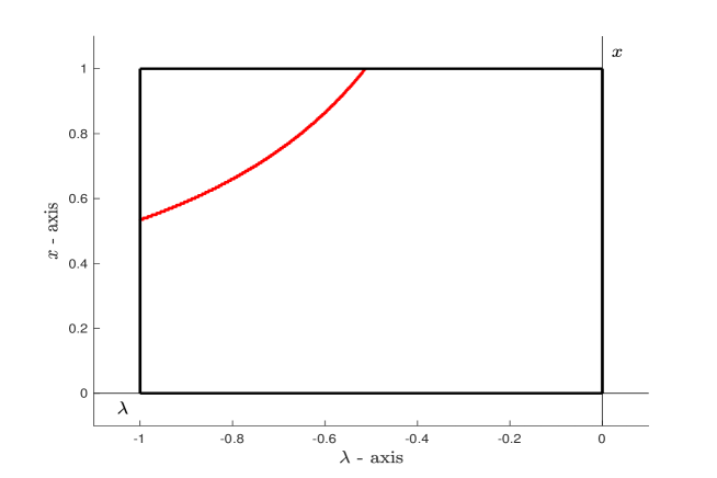
Figure 6.1: Full Maslov Box and spectral curve for (6.15).

6.2 Second-Order Systems

In this section, we consider eigenvalue problems of the general form

$$-B\phi^{\prime\prime}+W(x)\phi^{\prime}+V(x)\phi=\lambda\phi,\quad x\in(0,1),\quad\phi(x;\lambda)\in\mathbb{R}^{l},\quad l\in\mathbb{N},$$ (6.18)

for which we take $W,V\in C([0,1],\mathbb{R}^{l\times l})$ and assume for simplicity of the invariance verification that $B$ is a constant diagonal matrix with positive diagonal entries $\{b_{i}\}_{i=1}^{l}$. As noted in the introduction, such equations arise naturally when we linearize a viscous conservation law (1.3) about a viscous profile $\bar{u}(x-st)$.

In order to place this system in the setting of (1.1), we write $y={y_{1}\choose y_{2}}$ with $y_{1}=\phi$ and $y_{2}=B\phi^{\prime}$, giving (1.1) with $n=2l$ and

$$A(x;\lambda)=\begin{pmatrix}0&B^{-1}\\ V(x)-\lambda I&W(x)B^{-1}\end{pmatrix},$$ (6.19)

from which it’s clear that our Assumption (A) holds in this case. Computing directly, we see that

$$a_{ij}(x;\lambda_{2})-a_{ij}(x;\lambda)=\begin{cases}-(\lambda_{2}-\lambda)&(i,j)=(l+k,k),\,\,k\in\{1,\dots,l\}\\ 0&\textrm{otherwise},\end{cases}$$

allowing us to conclude that (B) holds as well. It follows that we can apply Theorem 1.1 as long as we can verify the invariance condition specified in Definition 1.2.

Following our general development, we fix any $m\in\{1,2,\dots,2l-1\}$ and let $\mathbf{G}(x;\lambda)\in\mathbb{R}^{2l\times m}$ and $\mathbf{H}(x;\lambda)\in\mathbb{R}^{2l\times(2l-m)}$ be as specified respectively in (1.11) and (1.12). Then

$$\tilde{\omega}_{1}(x;\lambda)=\det(\mathbf{G}(x;\lambda)\,\,\,\mathbf{H}(x;\lambda_{2})),$$

and

$$\tilde{\omega}_{2}(x;\lambda)=\sum_{i=1}^{2l}\tilde{\omega}^{i}_{2}(x;\lambda,\lambda_{1}),$$

where the functions $\{\tilde{\omega}^{i}_{2}(x;\lambda,\lambda_{1})\}_{i=1}^{2l}$ are as in (4.13).

For invariance, we will focus on the case $m=l$, for which the boundary spaces $\mathpzc{p}$ and $\mathpzc{q}$ from (1.2) both have the same dimension $l$, and we will consider two cases of boundary conditions. For this we will refer to $\mathpzc{p}$ or $\mathpzc{q}$ as a Robin space if it has a frame of the form ${I\choose\Phi}$ for some $l\times l$ matrix $\Phi$.

In the following proposition, $\mathpzc{f}(x;\lambda)$ denotes the Grassmannian subspace with frame $\mathbf{F}(x;\lambda)$ specified in (1.13), $\omega_{1}$ is specified in (1.14), and $\omega_{2}$ is specified in (1.16).

Proposition 6.2.

In (6.18), assume $W,V\in C([0,1],\mathbb{R}^{l\times l})$ and that $B$ is a constant diagonal matrix with positive diagonal entries $\{b_{i}\}_{i=1}^{l}$. For boundary spaces $\mathpzc{p}$ and $\mathpzc{q}$ as specified in (1.2), suppose $\mathpzc{p}$ is Dirichlet and $\mathpzc{q}$ is Robin, or alternatively suppose $\mathpzc{q}$ is Dirichlet and $\mathpzc{p}$ is Robin. Then there exists a value $r_{0}>0$ sufficiently small so that for any values $\{b_{i}\}_{i=1}^{l}$ satisfying

$$r:=\max\{\frac{1}{b_{1}},\frac{1}{b_{2}},\dots,\frac{1}{b_{n}}\}\leq r_{0},$$

we have $\rho(x;\lambda)>0$ for all $(x,\lambda)\in[0,1]\times[\lambda_{1},\lambda_{2}]$. In particular, the invariance condition specified in Definition 1.2 is satisfied for the triple $(\mathpzc{f}(\cdot;\cdot),\omega_{1},\omega_{2})$ on $[0,1]\times[\lambda_{1},\lambda_{2}]$, so $\mathfrak{m}=0$ in Theorem 1.1.

Proof.

Since the analysis is similar for each case, we carry out details only for the case in which (6.18) has Dirichlet boundary conditions at $x=1$ and Robin boundary conditions at $x=0$.

Following the general development of Section 5, we see immediately that the values $C_{a}$ and $C_{A}$ can be bounded independently of the values $\{b_{i}\}_{i=1}^{l}$ (for $r\leq r_{0}$). In order to apply our general framework, we additionally need to verify that the values $c_{g}$ and $c_{h}$ specified in (5.4) are bounded below uniformly as the values $\{b_{i}\}_{i=1}^{l}$ grow, and that by choosing the values $\{b_{i}\}_{i=1}^{l}$ sufficiently large we can make $\frac{\tilde{\omega}_{2}^{\prime}(x;\lambda)}{d(x;\lambda)}$ as small as we like (without increasing the value of $C$).

Beginning with the values $c_{g}$ and $c_{h}$, we notice that by regular perturbation theory for large values of $\{b_{i}\}_{i=1}^{l}$ the lowest order expression in a perturbation expansion for solutions of (1.1) with (6.19) solves the equation

$$y_{0}^{\prime}=A_{0}(x;\lambda)y_{0},\quad A_{0}(x;\lambda)=\begin{pmatrix}0&0\\ V(x)-\lambda I&0\end{pmatrix}.$$

For $\mathbf{G}(x;\lambda)$, we take the boundary condition $\mathbf{G}(0;\lambda)={I\choose\Theta}$, and if we let $\mathbf{G}_{0}(x;\lambda)={G_{0}(x;\lambda)\choose G_{00}(x;\lambda)}$ denote the lowest order term in a perturbation expansion for $\mathbf{G}(x;\lambda)$, then

$$G_{0}^{\prime}(x;\lambda)=0;\quad G_{0}(0;\lambda)=I;\quad\quad G_{00}^{\prime}(x;\lambda)=(V(x)-\lambda I)G_{0}(x;\lambda);\quad G_{00}(0;\lambda)=\Theta.$$

Solving this system by integration, we conclude that

$$\mathbf{G}_{0}(x;\lambda)=\begin{pmatrix}I\\ \mathcal{G}(x;\lambda)\end{pmatrix},\quad\mathcal{G}(x;\lambda)=\Theta+\int_{0}^{x}(V(\xi)-\lambda I)d\xi,$$ (6.20)

for all $x\in[0,1]$.

Likewise, for $\mathbf{H}(x;\lambda_{2})$, we take the boundary condition $\mathbf{H}(1;\lambda_{2})={0\choose I}$, and if we let $\mathbf{H}_{0}(x;\lambda_{2})={H_{0}(x;\lambda_{2})\choose H_{00}(x;\lambda_{2})}$ denote the lowest order term in a perturbation expansion for $\mathbf{H}(x;\lambda_{2})$, then

$$H_{0}^{\prime}(x;\lambda_{2})=0;\quad H_{0}(0;\lambda_{2})=0;\quad\quad H_{00}^{\prime}(x;\lambda_{2})=(V(x)-\lambda_{2}I)H_{0}(x;\lambda_{2});\quad H_{00}(0;\lambda_{2})=I.$$

Solving this system by integration, we conclude that

$$\mathbf{H}_{0}(x;\lambda_{2})=\begin{pmatrix}0\\ I\end{pmatrix},$$ (6.21)

for all $x\in[0,1]$.

Similarly as in the proof of Proposition 6.1, we can conclude that the values $c_{g}$ and $c_{h}$, viewed as functions of the values $\{b_{i}\}_{i=1}^{l}$, can be bounded below by positive constants that are independent of the value $r$ specified in Proposition 6.2 (as long as $r\leq r_{0}$), and likewise we can conclude that there exists a value $d_{\min}>0$, independent of the values $\{b_{i}\}_{i=1}^{n}$, so that

$$d(x;\lambda)\geq d_{\min},\quad\forall\,\,(x,\lambda,r)\in[0,1]\times[\lambda_{1},\lambda_{2}]\times[0,r_{0}].$$

Turning now to the ratio $\frac{\tilde{\omega}_{2}^{\prime}(x;\lambda)}{d(x;\lambda)}$, we first observe that in this case,

$$\mathcal{S}_{i}(\lambda,\lambda_{2})h_{j}:=\begin{cases}-(\lambda_{2}-\lambda)h_{i-l,j}&(i,j)\in\{l+1,\dots,2l\}\times\{1,\dots,l\}\\ 0&\textrm{otherwise},\end{cases}$$ (6.22)

from which we immediately see from (4.13) that $\tilde{\omega}_{2}^{i}(x;\lambda,\lambda_{1})\equiv 0$ for all $i\in\{1,2,\dots,l\}$. In order to understand the remaining functions $\{\tilde{\omega}^{i}_{2}(x;\lambda,\lambda_{1})\}_{i=l+1}^{2l}$ in this case, we focus on $i=l+1$ for which (from (4.13)) $\tilde{\omega}_{2}^{l+1}(x;\lambda,\lambda_{1})$ is the determinant of the matrix obtained by replacing the $(l+1)^{\textrm{th}}$ row of $(\mathbf{G}(x;\lambda)\,\,\mathbf{H}(x;\lambda_{2}))$ with

$$\begin{pmatrix}0&\dots&0&\mathcal{S}_{l+1}(\lambda_{1},\lambda_{2})h_{1}(\lambda_{2})&\dots&\mathcal{S}_{l+1}(\lambda_{1},\lambda_{2})h_{l}(\lambda_{2})\\ \end{pmatrix}$$

$$=\begin{pmatrix}0&\dots&0&-(\lambda_{2}-\lambda_{1})h_{11}(x;\lambda_{2})&\dots&-(\lambda_{2}-\lambda_{1})h_{1l}(x;\lambda_{2})\end{pmatrix}.$$

From this relation, and similar relations for $\{\tilde{\omega}_{2}^{i}(x;\lambda,\lambda_{1})\}_{i=l+2}^{2l}$ and $\{\tilde{\omega}_{2}^{i}(x;\lambda,\lambda)\}_{i=l+1}^{2l}$, we see that (5.8) is satisfied.

As in previous calculations along these lines, we compute the derivative of $\tilde{\omega}_{2}^{l+1}(x;\lambda,\lambda_{1})$ as the sum of $2l$ determinants, each with a derivative on each entry in exactly one row. The first of these determinants is

$$\det\begin{pmatrix}g_{11}^{\prime}(\lambda)&\dots&g_{1l}^{\prime}(\lambda)&h_{11}^{\prime}(\lambda_{2})&\dots&h_{1l}^{\prime}(\lambda_{2})\\ \vdots&\vdots&\vdots&\vdots&\vdots&\vdots\\ g_{l1}(\lambda)&\dots&g_{ll}(\lambda)&h_{l1}(\lambda_{2})&\dots&h_{ll}(\lambda_{2})\\ 0&\dots&0&-(\lambda_{2}-\lambda_{1})h_{11}(\lambda_{2})&\dots&-(\lambda_{2}-\lambda_{1})h_{1l}(\lambda_{2})\\ g_{(l+2)1}(\lambda)&\dots&g_{(l+2)l}(\lambda)&h_{(l+2)1}(\lambda_{2})&\dots&h_{(l+2)l}(\lambda_{2})\\ \vdots&\vdots&\vdots&\vdots&\vdots&\vdots\\ g_{(2l)1}(\lambda)&\dots&g_{(2l)l}(\lambda)&h_{(2l)1}(\lambda_{2})&\dots&h_{(2l)l}(\lambda_{2})\end{pmatrix}.$$ (6.23)

In this case,

$$g_{1j}^{\prime}=\frac{1}{b_{1}}g_{(l+1)j},\quad h_{1j}^{\prime}=\frac{1}{b_{1}}h_{(l+1)j},\quad\forall\,j\in\{1,2,\dots,l\},$$

and we see that (6.23) becomes

$$\frac{(\lambda_{2}-\lambda_{1})}{b_{1}}\det\begin{pmatrix}g_{(l+1)1}(\lambda)&\dots&g_{(l+1)l}(\lambda)&h_{(l+1)1}(\lambda_{2})&\dots&h_{(l+1)l}(\lambda_{2})\\ \vdots&\vdots&\vdots&\vdots&\vdots&\vdots\\ g_{l1}(\lambda)&\dots&g_{ll}(\lambda)&h_{l1}(\lambda_{2})&\dots&h_{ll}(\lambda_{2})\\ 0&\dots&0&-h_{11}(\lambda_{2})&\dots&-h_{1l}(\lambda_{2})\\ g_{(l+2)1}(\lambda)&\dots&g_{(l+2)l}(\lambda)&h_{(l+2)1}(\lambda_{2})&\dots&h_{(l+2)l}(\lambda_{2})\\ \vdots&\vdots&\vdots&\vdots&\vdots&\vdots\\ g_{(2l)1}(\lambda)&\dots&g_{(2l)l}(\lambda)&h_{(2l)1}(\lambda_{2})&\dots&h_{(2l)l}(\lambda_{2})\end{pmatrix}.$$ (6.24)

Using Hadamard’s inequality for determinants, we can bound this term by

$$\frac{\lambda_{2}-\lambda_{1}}{b_{1}}|g_{1}(x;\lambda)|\cdots|g_{l}(x;\lambda)||h_{1}(x;\lambda_{2})|\cdots|h_{l}(x;\lambda_{2})|.$$ (6.25)

For the next $(l-1)$ summands of $\partial_{x}\tilde{\omega}_{2}^{l+1}(x;\lambda,\lambda_{1})$, we similarly start with a derivative on the $j^{\rm th}$ row ($j\in\{2,\dots,l\}$) of the matrix under determinant in $\tilde{\omega}_{2}^{l+1}(x;\lambda,\lambda_{1})$. In each of these cases, the $j^{\rm th}$ row becomes linearly dependent with the $(l+j)^{\rm th}$ row, and the resulting determinant is 0. This brings us to the summand obtained by differentiating the $(l+1)^{\rm st}$ row of the matrix under determinant in $\tilde{\omega}_{2}^{l+1}(x;\lambda,\lambda_{1})$, and it’s straightforward to see that this term can again be estimated by (6.25).

In order to understand the determinants with derivatives on rows $l+2$ through $2l$, we focus on the first. For this, we have

$$\det \begin{pmatrix}g_{11}(\lambda)&\dots&g_{1l}(\lambda)&h_{11}(\lambda_{2})&\dots&h_{1l}(\lambda_{2})\\ \vdots&\vdots&\vdots&\vdots&\vdots&\vdots\\ g_{l1}(\lambda)&\dots&g_{ll}(\lambda)&h_{l1}(\lambda_{2})&\dots&h_{ll}(\lambda_{2})\\ 0&\dots&0&-(\lambda_{2}-\lambda_{1})h_{11}(\lambda_{2})&\dots&-(\lambda_{2}-\lambda_{1})h_{1l}(\lambda_{2})\\ g_{(l+2)1}^{\prime}(\lambda)&\dots&g_{(l+2)l}^{\prime}(\lambda)&h_{(l+2)1}^{\prime}(\lambda_{2})&\dots&h_{(l+2)l}^{\prime}(\lambda_{2})\\ \vdots&\vdots&\vdots&\vdots&\vdots&\vdots\\ g_{(2l)1}(\lambda)&\dots&g_{(2l)l}(\lambda)&h_{(2l)1}(\lambda_{2})&\dots&h_{(2l)l}(\lambda_{2})\end{pmatrix}$$

$$=\det\begin{pmatrix}g_{11}(\lambda)&\dots&g_{1l}(\lambda)&h_{11}(\lambda_{2})&\dots&h_{1l}(\lambda_{2})\\ \vdots&\vdots&\vdots&\vdots&\vdots&\vdots\\ g_{l1}(\lambda)&\dots&g_{ll}(\lambda)&h_{l1}(\lambda_{2})&\dots&h_{ll}(\lambda_{2})\\ 0&\dots&0&-(\lambda_{2}-\lambda_{1})h_{11}(\lambda_{2})&\dots&-(\lambda_{2}-\lambda_{1})h_{1l}(\lambda_{2})\\ a_{(l+2)k}g_{k1}(\lambda)&\dots&a_{(l+2)k}g_{kl}(\lambda)&a_{(l+2)k}h_{k1}(\lambda_{2})&\dots&a_{(l+2)k}h_{kl}(\lambda_{2})\\ \vdots&\vdots&\vdots&\vdots&\vdots&\vdots\\ g_{(2l)1}(\lambda)&\dots&g_{(2l)l}(\lambda)&h_{(2l)1}(\lambda_{2})&\dots&h_{(2l)l}(\lambda_{2})\end{pmatrix},$$

where for typesetting considerations we’re using the convention of summing over any index appearing twice in an expression. E.g., written out in full

$$a_{(l+2)k}g_{k1}(\lambda)=\sum_{k=1}^{2l}a_{(l+2)k}(x;\lambda)g_{k1}(x;\lambda),$$

and similarly for other such entries.

We can use row operations to eliminate all except two of the summands involving components of $\mathbf{G}(x;\lambda)$ in row $(l+1)$. In particular, we can eliminate all summands except

$$a_{(l+2)(l+1)}(x;\lambda)g_{(l+1)j}(x;\lambda)+a_{(l+2)(l+2)}(x;\lambda)g_{(l+2)j}(x;\lambda),\quad j=1,2,\dots,l.$$

For summands involving components of $\mathbf{H}(x;\lambda_{2})$, we correspondingly obtain sums of the form

$$a_{(l+2)(l+1)} (x;\lambda_{2})h_{(l+1)j}(x;\lambda_{2})+a_{(l+2)(l+2)}(x;\lambda_{2})h_{(l+2)j}(x;\lambda_{2})$$

$$+\sum_{k\notin\{(l+1),(l+2)\}}(a_{(l+2)k}(x;\lambda_{2})-a_{(l+2)k}(x;\lambda))h_{k1}(x;\lambda_{2}),\quad j=1,2,\dots,l.$$

Using (6.19), we see that

$$a_{(l+2)(l+1)}(x;\lambda)=(W(x)B^{-1})_{21}=\frac{W_{21}(x)}{b_{1}},\quad a_{(l+2)(l+2)}(x;\lambda)=(W(x)B^{-1})_{22}=\frac{W_{22}(x)}{b_{2}},$$ (6.26)

and similarly

$$\sum_{k\notin\{(l+1),(l+2)\}}(a_{(l+2)k}(x;\lambda_{2})-a_{(l+2)k}(x;\lambda))h_{kj}(x;\lambda_{2})=-(\lambda_{2}-\lambda)h_{2j},\quad j=1,2,\dots,l.$$ (6.27)

The terms (6.26) lead to an estimate by

$$\Big{(}\frac{|W_{21}(x)|}{b_{1}}+\frac{|W_{22}(x)|}{b_{2}}\Big{)}|g_{1}(x;\lambda)|\cdots|g_{l}(x;\lambda)||h_{1}(x;\lambda_{2})|\cdots|h_{l}(x;\lambda_{2})|,$$ (6.28)

while the remaining terms (6.27) lead to the determinant

$$\det\begin{pmatrix}g_{11}(\lambda)&\dots&g_{1l}(\lambda)&h_{11}(\lambda_{2})&\dots&h_{1l}(\lambda_{2})\\ \vdots&\vdots&\vdots&\vdots&\vdots&\vdots\\ g_{l1}(\lambda)&\dots&g_{ll}(\lambda)&h_{l1}(\lambda_{2})&\dots&h_{ll}(\lambda_{2})\\ 0&\dots&0&-(\lambda_{2}-\lambda_{1})h_{11}(\lambda_{2})&\dots&-(\lambda_{2}-\lambda_{1})h_{1l}(\lambda_{2})\\ 0&\dots&0&-(\lambda_{2}-\lambda)h_{21}(\lambda_{2})&\dots&-(\lambda_{2}-\lambda)h_{2l}(\lambda_{2})\\ g_{(l+3)1}(\lambda)&\dots&g_{(l+3)l}(\lambda)&h_{(l+3)1}(\lambda_{2})&\dots&h_{(l+3)l}(\lambda_{2})\\ \vdots&\vdots&\vdots&\vdots&\vdots&\vdots\\ g_{(2l)1}(\lambda)&\dots&g_{(2l)l}(\lambda)&h_{(2l)1}(\lambda_{2})&\dots&h_{(2l)l}(\lambda_{2})\end{pmatrix}.$$ (6.29)

To lowest order in $r$, we can compute this determinant with $\mathbf{G}(x;\lambda)$ and $\mathbf{H}(x;\lambda_{2})$ respectively approximated by $\mathbf{G}_{0}(x;\lambda)$ and $\mathbf{H}_{0}(x;\lambda_{2})$ as in (6.20) and (6.21). In this way, we obtain a determinant of the form

$$\det\begin{pmatrix}I&0\\ \tilde{\mathcal{G}}(x;\lambda)&\tilde{I}\end{pmatrix}=\det(\tilde{I}).$$

where the temporary notation $\tilde{\mathcal{G}}(x;\lambda)$ signifies the matrix obtained by taking the first two rows of $\mathcal{G}(x;\lambda)$ to be identically zero while leaving all other rows unchanged, and likewise $\tilde{I}$ signifies the matrix obtained by taking the first two rows of $I$ to be identically zero while leaving all other rows unchanged. Since $\det(\tilde{I})=0$, we can conclude that the full determinant (6.29) is order $r$.

These details have been carried out for the single term $\tilde{\omega}_{2}^{l+1}(x;\lambda,\lambda_{1})$, and only for the cases in which derivatives appear on one of the first $l+2$ rows. However, the analysis of the terms with derivatives on the remaining rows, and the analysis of the remaining terms $\{\tilde{\omega}_{2}^{i}(x;\lambda,\lambda_{1})\}_{i=l+2}^{2l}$ introduces no additional complications, and we can conclude that there exists a constant $K>0$, independent of the values $\{b_{i}\}_{i=1}^{l}$, so that

$$\tilde{\omega}_{2}^{\prime}(x;\lambda)\leq Kr,$$

and consequently

$$|\frac{\tilde{\omega}_{2}^{\prime}(x;\lambda)}{d(x;\lambda)}|\leq\frac{Kr}{d_{\min}}.$$

In our general invariance relation (5.11), we can now take $C$ as specified in Lemma 5.1, with

$$C_{d} =\frac{l!C_{A}}{c_{g}^{2}}+\frac{l!}{c_{h}^{2}}\max_{x\in[0,1]}\|A(x;\lambda_{2})\|$$

$$\delta =\frac{Kr}{d_{\min}}$$

keeping in mind that $C_{a}$ and $C_{A}$ can both be bounded independently of the values $\{b_{i}\}_{i=1}^{l}$. Since $C$ can be taken independent of the values $\{b_{i}\}_{i=1}^{l}$, and $\delta$ can be taken as small as we like by decreasing $r$, we can ensure (5.11) holds so long as we can show that $\rho(0;\lambda)$ remains bounded away from 0 as $r$ decreases.

For this final point, we recall that $\rho(0;\lambda)$ can be expressed as

$$\rho(0;\lambda)=\frac{1}{2d(0;\lambda)^{2}}(\tilde{\omega}_{1}(0;\lambda)^{2}+\tilde{\omega}_{2}(0;\lambda)^{2}).$$

We can compute this value to lowest order in $r$ by using the frames $\mathbf{G}(0;\lambda)={I\choose\Theta}$ and $\mathbf{H}(0;\lambda_{2})={0\choose I}$. We see immediately that

$$\tilde{\omega}_{1}(0;\lambda)=\det\begin{pmatrix}I&0\\ \Theta&I\end{pmatrix}=\det I=1,$$

from which we can conclude that to lowest order in $r$

$$\rho(0;\lambda)\geq\frac{1}{2d_{\min}^{2}}.$$

∎

6.2.1 Example Case with Invariance

In this section, we will apply Theorem 1.1 to (6.18) with $l=2$, taking specifically $B$ to be the $2\times 2$ identity matrix and

$$V(x)=\begin{pmatrix}10\sin(10x)\cos(10x)&25\sin(10x)\\ x(1-x)&10\cos(10x)\end{pmatrix},\quad W(x)=\begin{pmatrix}5x(1-x)&0\\ 0&5x(1-x)\end{pmatrix},$$ (6.30)

along with Neumann boundary conditions at both $x=0$ and $x=1$. For Neumann conditions, it’s natural to take the frames for $\mathpzc{p}$ and $\mathpzc{q}$ to both be ${I\choose 0}$. For this example, we are not taking the entries of $B$ to be large, and in addition we are not using boundary conditions allowed by Proposition 6.2, so we do not have an a priori guarantee of invariance. Nonetheless, we will (numerically) check invariance by computing $\rho(x;\lambda)$ throughout (a grid on) the full Maslov box (including the interior). Indeed, one of our goals with this example is to illustrate that there is an enormous gap between systems for which we have rigorously verified invariance and systems for which invariance holds.

We will count the number of eigenvalues the system (6.18)–(6.30) has on the interval $[\lambda_{1},\lambda_{2}]=[-5,1]$. For this, we compute $\operatorname{Ind}(\mathpzc{g}(\cdot;-5),\mathpzc{h}(\cdot;1);[0,1])$, and we find two crossing points, at about $x=.043$ and $x=.455$ (with a stepsize in the computation of $.001$). If the system is known to be invariant on $[0,1]\times[-5,1]$ then we can conclude that (6.18)–(6.30) has at least two eigenvalues on the interval $[-5,1]$. This is the most information that we can get out of Theorem 1.1 for this example, but computationally, we find approximately that

$$\min_{\underset{\lambda\in[\lambda_{1},\lambda_{2}]}{x\in[0,1]}}\rho(x;\lambda)=.6279,$$

suggesting that invariance indeed holds. The full Maslov box for this example is depicted in Figure 6.2. The eigenvalues are at roughly $\lambda=-1.385$ and $\lambda=.735$ (with a stepsize in the computation of $.0025$).

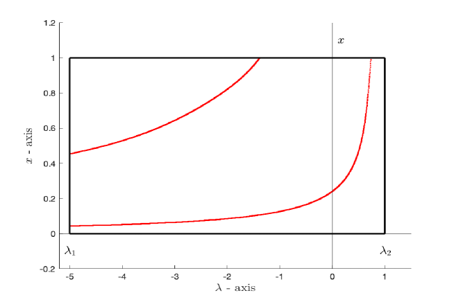
Figure 6.2: Full Maslov Box and spectral curves for (6.18)–(6.30).

6.2.2 Example Case without Invariance

An enormous amount remains to be said about invariance, and as a point of interest, we compute the full Maslov box for a case in which invariance fails to hold at precisely two points in the interior of the Maslov box. For this example, we’ll take (6.18) with $l=2$, taking again $B$ to be the $2\times 2$ identity matrix and choosing

$$V(x)=\begin{pmatrix}10\sin(10x)\cos(10x)&25\sin(10x)\\ x(1-x)&10\cos(10x)\end{pmatrix},\quad W(x)=\begin{pmatrix}5x(1-x)&10\sin(10x)\\ 10\cos(10x)&5x(1-x)\end{pmatrix},$$ (6.31)

along with Neumann boundary conditions at both $x=0$ and $x=1$.

For the system (6.18)–(6.31), we find by numerical computation that $\rho(x;\lambda)$ has two zeros in the interior of the Maslov box $[0,1]\times[-5,1]$, approximately at the points $(.875,-3.348)$ and $(.875,-.130)$. This suggest that invariance fails in this case. The full Maslov box for this example is depicted in Figure 6.3. On the left-hand side of the figure, the Maslov box is drawn for $[\lambda_{1},\lambda_{2}]=[-5,1]$, and we see that the associated spectral curve is a loop contained entirely in the interior of the Maslov box, with left-most and right-most points corresponding precisely with zeros of $\rho(x;\lambda)$. Since no spectral curves intersect the boundary of the Maslov box, it’s clear that $\mathfrak{m}=0$, and it’s interesting to understand how we can see this from the local considerations discussed in Section 2.2. To this end, we consider the contribution to $\mathfrak{m}$ from each of the points at which invariance is lost. First, at $(.875,-3.348)$, Figure 6.3 suggests that the spectral curve can be expressed as a functional relation $\lambda=\lambda(x)$, with $\lambda^{\prime}(.875)=0$, and we have precisely the situation of the middle plot in Figure 2.1 (with $\lambda$ now in place of $s$ and $x$ in place of $t$). As in the discussion in Section 2.2, we can conclude that the contribution to $\mathfrak{m}$ from this point is $+2$. The second point at which invariance is lost is $(.875,-.130)$, and again we see that near this point the spectral curve can be expressed as a functional relation $\lambda=\lambda(x)$, with $\lambda^{\prime}(.875)=0$. In this case, we have precisely the situation of the left-side plot in Figure 2.1, and can conclude that the contribution to $\mathfrak{m}$ from this point is $-2$. Since there are no other points of invariance, the total generalized Maslov index along the boundary is $\mathfrak{m}=+2+(-2)=0$. Using this information in our application of Theorem 1.1, we can write

$$\mathcal{N}_{\#}([-5,1])\geq|\#\{x\in(0,L]:\mathpzc{g}(x;0)\cap\mathpzc{q}\neq\{0\}\}+\mathfrak{m}|=0.$$

In fact, it’s clear from the full Maslov box that $\mathcal{N}_{\#}([-5,1])=0$.

Turning to the Maslov box on the right-hand side of Figure 6.3, we see again that we have invariance along the boundary of the Maslov box. (Here, we recall that invariance is only lost on the right and left endpoints of the spectral curves.) By monotonicity, each of the crossing points along the left shelf gives a contribution to the generalized Maslov index of $-1$, so $\mathfrak{m}=-2$. Again, it’s interesting to see that we can identify this value from local information. In this case, the only point in the Maslov box at which invariance is lost is $(.875,-.130)$, and we have already seen that its contribution to $\mathfrak{m}$ will be $-2$. Since there are no other contributions to $\mathfrak{m}$ in this case, we conclude that $\mathfrak{m}=-2$. Using this information in our application of Theorem 1.1, we can write

$$\mathcal{N}_{\#}([-3,1])\geq|\#\{x\in(0,L]:\mathpzc{g}(x;0)\cap\mathpzc{q}\neq\{0\}\}+(-2)|=0.$$

In fact, it’s clear from the full Maslov box that $\mathcal{N}_{\#}([-3,1])=0$.

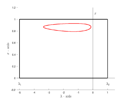
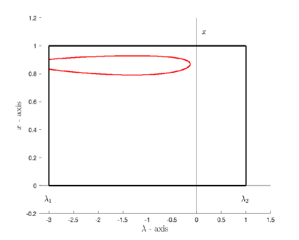
Figure 6.3: Spectral curves for the system (6.18)–(6.31).

Acknowledgements. The author is grateful to Graham Cox for patiently answering numerous questions about [2].

References

• [1] V. I. Arnol’d, The Sturm theorems and symplectic geometry, Fund. Anal. Appl. 19 (1985) 251-259.
• [2] T. J. Baird, P. Cornwell, G. Cox, C. Jones, and R. Marangell, Generalized Maslov indices for non-Hamiltonian systems, SIAM J. Math. Anal. 54 (2022) 1623-1668.
• [3] M. Bohner, W. Kratz, and R. Šimon Hilscher, Oscillation and spectral theory for linear Hamiltonian systems with nonlinear dependence on the spectral parameter, Nath. Nachr. 285 (11–12) (2012) 1343–1356.
• [4] V. Barutello, D. Offin, A. Portaluri, and L. Wu, Sturm theory with applications in classical mechanics, Preprint 2020, arXiv: 2005.08034.
• [5] F. Chardard and T. J. Bridges, Transversality of homoclinic orbits, the Maslov index, and the symplectic Evans function, Nonlinearity 28 (2015) 77–102.
• [6] G. Cox, C. K. R. T. Jones, Y. Latushkiun, and A. Sukhtayev, The Morse and Maslov indices for multidimensional Schrödinger operators with matrix-valued potentials, Trans. Amer. Math. Soc. 368 (2016) 8145-8207.
• [7] M. De Gosson, S. De Gosson, and P. Piccione, On a product formula for the Conley-Zehnder index of symplectic paths and its applications, Ann. Glob. Anal. Geom. 34 (2008) 167–183.
• [8] J. Deng and C. Jones, Multi-dimensional Morse Index Theorems and a symplectic view of elliptic boundary value problems, Trans. Amer. Math. Soc. 363 (2011) 1487 – 1508.
• [9] H. M. Edwards, A generalized Sturm theorem, Ann. Math 80 (1964) 22-57.
• [10] J. Elyseeva, Renormalized oscillation theory for symplectic eigenvalue problems with nonlinear dependence on the spectral parameter, J. Differ. Equ. Appl. 26 (2020) 458-487.
• [11] K. Furutani, Fredholm-Lagrangian-Grassmannian and the Maslov index, Journal of Geometry and Physics 51 (2004) 269 – 331.
• [12] F. Gesztesy, B. Simon, and G. Teschl, Zeros of the Wronskian and renormalized oscillation theory, American J. Math. 118 (1996) 571–594.
• [13] F. Gesztesy and M. Zinchenko, Renormalized oscillation theory for Hamiltonian systems, Adv. Math. 311 (2017) 569–597.
• [14] P. Howard, Asymptotic behavior near transition fronts for equations of generalized Cahn-Hilliard form, Commun. Math. Phys. 269 (2007) 765–808.
• [15] P. Howard, Hörmander’s index and oscillation theory, J. Math. Anal. Appl. (500) (2021) 1 – 38.
• [16] P. Howard and A. Sukhtayev, The Maslov and Morse indices for Schrödinger operators on [0, 1], J. Differential Equations 260 (2016) 4499-4549.
• [17] P. Howard and A. Sukhtayev, Renormalized oscillation theory for linear Hamiltonian systems on $[0,1]$ via the Maslov index, J. Dynamics and Differential Equations, DOI: 10.1007/s10884-021-10121-2.
• [18] P. Howard and A. Sukhtayev, Renormalized oscillation theory for singular linear Hamiltonian systems, J. Functional Analysis 283 (2022).
• [19] P. Howard and K. Zumbrun, Pointwise estimates and stability for dispersive–diffusive shock waves, Arch. Rational Mech. Anal. 155 (2000) 85–169.
• [20] R. L. Pego and M. I. Weinstein, Eigenvalues, and instabilities of solitary waves, Phil. Trans. R. Soc. Lond. A 340 (1992) 47-94.
• [21] H. Schulz-Baldes, Sturm intersection theory for periodic Jacobi matrices and linear Hamiltonian systems, Linear Algebra Appl. 436 (2012) 498 – 515.
• [22] B. Simon, Sturm oscillation and comparison theorems, in Sturm-Liouville Theory: Past and Present, Birkhäuser Verlag 2005, W. O. Amrein, A. M. Hinz, and D. B. Pearson, Eds.
• [23] G. Teschl, Oscillation theory and renormalized oscillation theory for Jacobi operators, J. Differential Equations 129 (1996) 532–558.
• [24] G. Teschl, Renormalized oscillation theory for Dirac operators, Proceedings of the AMS 126 (1998) 1685–1695.
• [25] K. Zumbrun and P. Howard, Pointwise semigroup methods and stability of viscous shock waves, Indiana U. Math. J. 47 (1998) 741-871. See also the errata for this paper: Indiana U. Math. J. 51 (2002) 1017–1021.