Consistency between the attached-eddy model and the inner-outer interaction model: a study of streamwise wall-shear stress fluctuations in a turbulent channel flow

Abstract

The inner-outer interaction model (Marusic, Mathis & Hutchins, Science, vol. 329, 2010, 193-196) and the attached-eddy model (Townsend, Cambridge University Press, 1976) are two fundamental models describing the multi-scale turbulence interactions and the organization of energy-containing motions in the logarithmic region of high-Reynolds number wall-bounded turbulence, respectively. In this paper, by coupling the additive description with the attached-eddy model, the generation process of streamwise wall-shear fluctuations, resulting from wall-attached eddies, is portrayed. Then, by resorting to the inner-outer interaction model, the streamwise wall-shear stress fluctuations generated by attached eddies in a turbulent channel flow are isolated. Direct comparison between the statistics from these two models demonstrates that they are consistent to and complement each other. Meanwhile, we further show that the superpositions of attached eddies follow an additive process strictly by verifying the validity of the strong and extended self similarity. Moreover, we propose a Gaussian model to characterize the instantaneous distribution of streamwise wall-shear stress, resulting from the attached-eddy superpositions. These findings are important for developing an advanced reduced-order wall model.

MSC Codes (Optional) Please enter your MSC Codes here

1 Introduction

Wall-shear stress fluctuation is a crucial physical quantity in wall-bounded turbulence, as it is of importance for noise radiation, structural vibration, drag generation, and wall heat transfer, among others (Diaz-Daniel et al., 2017; Cheng et al., 2020). In the past two decades, ample evidence has shown that the root mean squared value of streamwise wall-shear stress fluctuations ($\tau_{x,rms}^{{}^{\prime}}$) is sensitive to the flow Reynolds number (Abe et al., 2004; Schlatter & Örlü, 2010; Yang & Lozano-Durán, 2017; Guerrero et al., 2020). It indicates that large-scale energy-containing eddies populating the logarithmic and outer regions in high-Reynolds-number wall turbulence have non-negligible influences on the near-wall turbulence dynamics, and thus the wall friction (de Giovanetti et al., 2016; Li et al., 2019).

Till now, several models have been proposed on the organization of motions in logarithmic and outer regions and their interactions with the near-wall dynamics. Marusic et al. (2010) have established that superposition and modulation are the two basic mechanisms that large-scale motions (LSM) and very-large-scale motions (VLSM) exert influences on the near-wall turbulence. The former refers to the footprints of LSMs and VLSMs on the near-wall turbulence, while the latter indicates the intensity amplification or attenuation of near-wall small-scale turbulence by the outer motions. Mathis et al. (2013) extended the model to interpret the generation of wall-shear stress fluctuations in high-Reynolds number flows. They emphasized that superposition and modulation are still two essential factors. This inner-outer interaction model (IOIM) has also been successfully developed to predict the near-wall velocity fluctuations with data inputs from the log layer (Marusic et al., 2010; Baars et al., 2016; Wang et al., 2021).

On the other hand, the most elegant conceptual model describing the motions in logarithmic region is the attached-eddy model (AEM) (Townsend, 1976; Perry & Chong, 1982). It conjectures that the logarithmic region is occupied by an array of self-similar energy-containing motions (or eddies) with their roots attached to the near-wall region. Extensive validations support the existence of attached eddies in high-Reynolds number turbulence, such as the logarithmic decaying of streamwise velocity fluctuation intensities (Meneveau & Marusic, 2013), as originally predicted by Townsend (1976). The reader is referred to a recent review work by Marusic & Monty (2019) for more details. Given the existence of wall-attached energy-containing motions in the logarithmic region, it would be quite natural to hypothesize that the near-wall part of these motions would affect the generation of the wall-shear fluctuations to some extent, maybe, via the superposition and modulation mechanisms. However, some fundamental questions may be raised, e.g., whether the IOIM and AEM are consistent with each other? There’s a possibility that the superposition component of $\tau_{x}^{\prime}$ decomposed by the IOIM in physical space can not fully follow the predictions made by the AEM quantitatively. If yes, whether these two models can shed light on the mechanism of wall-shear fluctuation generation and be indicative for modeling approaches?

Previous study (Yang & Lozano-Durán, 2017) verified that the generation of wall-shear stress fluctuations can be interpreted as the outcomes of the momentum cascade across momentum-carried eddies of different scales, and modeled by an additive process. Here, we first aim to couple the additive description with the AEM to portray the generation process of streamwise wall-shear fluctuations, resulting from wall-attached eddies. Two scaling laws describing their intensities and the linkages with the characteristic scales of attached eddies can be derived (the characteristic scales of attached eddies are their wall-normal heights according to AEM (Townsend, 1976)). Then, we intend to isolate the streamwise wall-shear stress fluctuations generated by attached eddies in a turbulent channel flow at $Re_{\tau}=2003$ ($Re_{\tau}=hu_{\tau}/\nu$, $h$ denotes the channel half-height, $u_{\tau}$ the wall friction velocity and $\nu$ the kinematic viscosity) by resorting to the IOIM (Marusic et al., 2010; Baars et al., 2016). Here, IOIM is employed as a tool to estimate the streamwise wall-shear fluctuations generated by attached eddies. The statistics from IOIM can be processed to verify the scaling laws deduced by AEM, so as to demonstrate their consistency. Moreover, a simple algebraic model describing the instantaneous distributions of the streamwise wall-shear stress fluctuations generated by attached eddies will be proposed.

2 Streamwise wall-shear stress fluctuations generated by attached eddies

According to Mandelbrot (1974) and Yang & Lozano-Durán (2017), the generation of streamwise wall-stress fluctuations can be modeled as an additive process within multifractal formalism, which takes the form of

$$\tau_{x}^{{}^{\prime}+}=\sum_{i=1}^{n}a_{i},$$ (1)

where $a_{i}$ are random addends, representing an increment in $\tau_{x}^{{}^{\prime}+}$ due to eddies with wall-normal height $h/2^{i}$, and superscript $+$ denotes the normalization with wall units. Here, we intend to isolate the contributions from the eddies populating logarithmic region ($\tau_{x,o}^{{}^{\prime}+}$) and link to their wall-normal positions $y$. $\tau_{x,o}^{{}^{\prime}+}$ can be expressed as

$$\tau_{x,o}^{{}^{\prime}+}=\sum_{i=n_{s}}^{n_{o}}a_{i},$$ (2)

where $n_{s}$ and $n_{o}$ represent the additives that correspond to the eddies with the wall-normal height at $y_{s}$ and $y_{o}$, respectively. Here, $y_{s}$ is the lower bound of logarithmic region, and generally believed to be $80\leq y_{s}^{+}\leq 100$ (Jiménez, 2018; Baars & Marusic, 2020); $y_{o}$ is the outer reference height. It can be found that $1\textless n_{s}\textless n_{o}\textless n$. The addends $a_{i}$ are assumed to be identically and independently distributed (i.i.d) and equal to $a$. The number of the addends should be proportional to

$$n_{o}-n_{s}+1\sim\int_{y_{s}}^{y_{o}}p(y)dy\sim\int_{y_{s}}^{y_{o}}\frac{1}{y}dy\sim\ln(\frac{y_{o}}{y_{s}}),$$ (3)

where $p(y)$ is the eddy population density, which is proportional to $1/y$ according to AEM (Townsend, 1976; Perry & Chong, 1982). A momentum generation function $\left\langle exp(q\tau_{x,o}^{{}^{\prime}+})\right\rangle$, where $<>$ represents the averaging in the temporal and spatially homogeneous directions, is defined to scrutinize the scaling behavior of $\tau_{x,o}^{{}^{\prime}+}$ (Yang et al., 2016). $\left\langle exp(q\tau_{x,o}^{{}^{\prime}+})\right\rangle$ can be evaluated as

$$\left\langle exp(q\tau_{x,o}^{{}^{\prime}+})\right\rangle=\left\langle exp(qa)\right\rangle^{n_{o}-n_{s}+1}\sim(\frac{y_{o}}{y_{s}})^{s(q)},$$ (4)

where $q$ is a real number, $s(q)=C_{1}\ln\left\langle exp(qa)\right\rangle$ is called anomalous exponent, $C_{1}$ is a constant. Eq. (4) is called strong self similarity (SSS). If $a$ is a Gaussian variable, the anomalous exponent can be recast as

$$s(q)=C_{2}q^{2},$$ (5)

where $C_{2}$ is another constant. On the other hand, an extended self-similarity (ESS) is defined to describe the relationship between $\left\langle exp(q\tau_{x,o}^{{}^{\prime}+})\right\rangle$ and $\left\langle exp(q_{0}\tau_{x,o}^{{}^{\prime}+})\right\rangle$ (fixed $q_{0}$) (Benzi et al., 1993), i.e.,

$$\left\langle exp(q\tau_{x,o}^{{}^{\prime}+})\right\rangle=\left\langle exp(q_{0}\tau_{x,o}^{{}^{\prime}+})\right\rangle^{\xi(q,q_{0})},$$ (6)

where $\xi(q,q_{0})$ is a function of $q$ (fixed $q_{0}$). Note that ESS does not strictly rely on i.i.d of the addends, but the additive process Eq. (2).

3 DNS database and scale decomposition method

The direct numerical simulation (DNS) database used in the present study is an incompressible turbulent channel flow at $Re_{\tau}=2003$, which has been extensively validated by previous studies (Hoyas & Jiménez, 2006; Jiménez & Hoyas, 2008). The decomposition of $\tau^{\prime}_{x}$ is based on the IOIM first proposed by Marusic et al. (2010). Baars et al. (2016) modified the computational process by introducing spectral stochastic estimation to avoid artificial scale decomposition. In this work, the modified version of IOIM is adopted to investigate the multi-scale characteristics of $\tau^{\prime}_{x}$. It can be expressed as

$$u_{p}^{+}\left(y^{+}\right)=\underbrace{u^{*}\left(y^{+}\right)\left\{1+\Gamma_{uu}u_{L}^{+}\left(y^{+}\right)\right\}}_{u_{s}^{+}}+u_{L}^{+}\left(y^{+}\right),$$ (7)

where $u_{p}^{+}$ denotes the predicted near-wall streamwise velocity fluctuation, $u^{*}$ denotes the universal velocity signal without large-scale impact, $u_{L}^{+}$ is the superposition component, $\Gamma_{uu}$ is the amplitude-modulation coefficient, and $u_{s}^{+}$ denotes the amplitude modulation of the universal signal $u^{*}$. $u_{L}^{+}$ is obtained by spectral stochastic estimation of the streamwise velocity fluctuation at the logarithmic region $y_{o}^{+}$, namely,

$$u_{L}^{+}\left(x^{+},y^{+},z^{+}\right)=F_{x}^{-1}\left\{H_{L}\left(\lambda_{x}^{+},y^{+}\right)F_{x}\left[u_{o}^{+}\left(x^{+},y_{o}^{+},z^{+}\right)\right]\right\}$$ (8)

where $u_{o}^{+}$ is the streamwise velocity fluctuation at $y_{o}^{+}$ in the logarithmic region, and, $F_{x}$ and $F_{x}^{-1}$ denote FFT and inverse FFT in the streamwise direction, respectively. $H_{L}$ is the transfer kernel, which evaluates the correlation between $u^{+}(y^{+})$ and $u_{o}^{+}(y_{o}^{+})$ at a given length scale $\lambda_{x}^{+}$, and can be calculated as

$$H_{L}\left(\lambda_{x}^{+},y^{+}\right)=\frac{\left\langle\hat{u}\left(\lambda_{x}^{+},y^{+},z^{+}\right)\overline{\hat{u}_{o}}\left(\lambda_{x}^{+},y_{o}^{+},z^{+}\right)\right\rangle}{\left\langle\hat{u}_{o}\left(\lambda_{x}^{+},y_{o}^{+},z^{+}\right)\overline{\hat{u}_{o}}\left(\lambda_{x}^{+},y_{o}^{+},z^{+}\right)\right\rangle},$$ (9)

where $\hat{u}$ is the Fourier coefficient of $u$, and $\overline{\hat{u}}$ is the complex conjugate of $\hat{u}$.

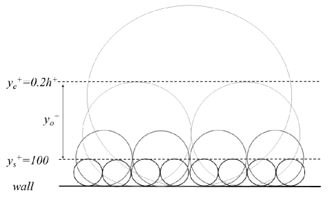
Figure 1: A schematic of the attached-eddy model (Hwang, 2015). Each circle represents an individual attached eddy. $y_{s}^{+}$ and $y_{e}^{+}$ are the lower and upper bound of the logarithmic region, respectively. $y_{0}^{+}$ is the outer reference height, and varies from $y_{s}^{+}$ to $y_{e}^{+}$.

In this work, we mainly pay attention to the quantity, $\tau^{\prime}_{x}$ generated by the attached eddies. Thus, the predicted position $y^{+}$ is fixed at $y^{+}=0.3$, and the outer reference height $y_{o}^{+}$ varies from $100$ (namely $y_{s}^{+}$) to $0.2h^{+}$ (denoted as $y_{e}^{+}$), i.e., the upper boundary of logarithmic region (Jiménez, 2018). We have checked that as long as the predicted position is around $y^{+}\leq O(1)$, the results presented below are insensitive to the choice of specific $y^{+}$. Once $u_{L}^{+}$ is obtained, the superposition component of $\tau_{x}^{{}^{\prime}+}$ can be calculated by definition (i.e., $\frac{\partial u_{L}^{{}^{\prime}+}}{\partial y^{+}}$ at the wall) and denoted as $\tau_{x,L}^{{}^{\prime}+}(y_{o}^{+})$. According to the hierarchical attached eddies in high-Reynolds number wall turbulence (see Fig. 1), $\tau_{x,L}^{{}^{\prime}+}(y_{o}^{+})$ represents the superposition contributed from the wall-coherent motions with their height larger than $y_{o}^{+}$. Thus, the difference value $\tau_{x,L}^{{}^{\prime}+}(y_{s}^{+})-\tau_{x,L}^{{}^{\prime}+}(y_{o}^{+})$ can be interpreted as the superposition contribution generated by the wall-coherent eddies with their wall-normal heights within $y_{s}^{+}$ and $y_{o}^{+}$, i.e., $\tau_{x,o}^{{}^{\prime}+}$ in Eq. (2). Considering that $y_{s}^{+}$ is the lower bound of the logarithmic region, the increase of $y_{o}^{+}$ corresponds to the enlargement of the addends in the additive description (see Eq. (2)). In this way, the connection between AEM and IOIM are established, and the AEM predictions (see Eqs. (4)-(6)) can be verified directly.

4 Results and discussion

4.1 Scaling laws of $\tau_{x,o}^{{}^{\prime}+}$

Figure 2: ($a$) $G$ as functions of $y_{o}/y_{s}$ for $q=\pm 5$ and $q=\pm 3$; ($b$) premultiplied $G$ as functions of $y_{o}/y_{s}$ for $q=\pm 5$ and $q=\pm 3$.

Here, we further define a moment generation function based on the IOIM, i.e.,

$$G(q,y_{o}^{+})=\left\langle exp(q(\tau_{x,L}^{{}^{\prime}+}(y_{s}^{+})-\tau_{x,L}^{{}^{\prime}+}(y_{o}^{+})))\right\rangle.$$ (10)

Fig. 2($a$) shows the variations of $G$ as a function of $y_{o}/y_{s}$ for $q=\pm 5$ and $q=\pm 3$. Power-law behaviours can be found in the interval between $1.7\leq y_{o}/y_{s}\leq 2.9$ for positive $q$ and $1.7\leq y_{o}/y_{s}\leq 4$ for negative $q$, justifying the validity of SSS, i.e., Eq. (4). Fig. 2 is in aid of accessing the scalings by displaying the variations of premultiplied $G$. This observation highlights that the superpositions of wall-attached log-region motions on wall surface follow the additive process, characterized by Eq. (2). It is also worth mentioning that the power-law behaviour can be observed for larger wall-normal intervals for negative $q$. As $G(q,y_{o}^{+})$ quantifies $\tau_{x,L}^{{}^{\prime}+}(y_{s}^{+})-\tau_{x,L}^{{}^{\prime}+}(y_{o}^{+})$, which features the same sign as $q$, this observation is consistent with the work of Cheng et al. (2020), which showed that the footprints of the inactive part of attached eddies populating the logarithmic region are actively connected with large-scale negative $\tau^{\prime}_{x}$. Other $q$ values yield similar results and are not shown here for brevity.

Figure 3: ($a$) Anomalous exponent $s(q)$ as a function of $q$. The black line is a quadratic fit; ($b$) second- to sixth- order moments of $\tau_{x}^{{}^{\prime}+}$ as functions of $Re_{\tau}$. The dashed lines are the log-normal predictions from Eq. (11)-(13).

The anomalous exponent $s(q)$ can be obtained by fitting the range $2\leq y_{o}/y_{s}\leq 2.9$, where both positive and negative $q$ display good power-law scalings. Fig. 3($a$) displays the variation of the anomalous exponent $s(q)$ as a function of $q$. The solid line denotes the quadratic fit within $-0.5\leq q\leq 0.5$. It can be seen that the variation of $s(q)$ is very close to the model prediction, i.e., the quadratic function as Eq. (5) with $C_{2}=0.00629$. Only minor discrepancies between DNS data and model predictions can be observed. As such, it is reasonable to hypothesize that the streamwise wall-shear stress fluctuation $\tau^{\prime}_{x}$ generated by attached eddies of a given size follows the Gaussian distribution. Moreover, we can also estimate the statistical moments of $\tau_{x,o}^{+}$ by taking the derivative of $G(q,y_{e}^{+})$ with respect to $q$ around $q=0$ (Yang et al., 2016), i.e.,

$$\left\langle\tau_{x,o}^{{}^{\prime}2+}\right\rangle=\left.\frac{\partial^{2}G(q;y_{o}^{+})}{\partial q^{2}}\right|_{q=0}\sim 2C_{2}\ln(y_{o}/y_{s})\sim 2C_{2}\ln Re_{\tau},$$ (11)

$$\left\langle\tau_{x,o}^{{}^{\prime}4+}\right\rangle^{1/2}=(\left.\frac{\partial^{4}G(q;y_{o}^{+})}{\partial q^{4}}\right|_{q=0})^{1/2}\sim 2\sqrt{3}C_{2}\ln(y_{o}/y_{s})\sim 2\sqrt{3}C_{2}\ln Re_{\tau},$$ (12)

$$\left\langle\tau_{x,o}^{{}^{\prime}6+}\right\rangle^{1/3}=(\left.\frac{\partial^{6}G(q;y_{o}^{+})}{\partial q^{6}}\right|_{q=0})^{1/3}\sim 2\sqrt[3]{15}C_{2}\ln(y_{o}/y_{s})\sim 2\sqrt[3]{15}C_{2}\ln Re_{\tau}.$$ (13)

Fig. 3($b$) shows the variations of second- ($p=1$) to sixth- ($p=3$) order moments of $\tau^{\prime}_{x}$ calculated from DNS of channel flows (Iwamoto et al., 2002; Del Álamo & Jiménez, 2003; Abe et al., 2004; Del Álamo et al., 2004; Hu et al., 2006; Lozano-Durán & Jiménez, 2014; Lee & Moser, 2015; Cheng et al., 2019; Kaneda & Yamamoto, 2021) and compares them with the model prediction, i.e., Eq. (11)-(13). For the second- and fourth- order variances, the model predictions are roughly consistent with the DNS results. The comparisons also indicate a Reynolds-number dependence of $\left\langle\tau_{x}^{{}^{\prime}2+}\right\rangle$, which has been reported by vast studies (Schlatter & Örlü, 2010; Mathis et al., 2013; Guerrero et al., 2020), and may be ascribed to the superposition effects of the wall-attached log-region motions. Wang et al. (2020) speculated that the amplitude modulation effect plays a more prominent role in affecting the statistic characteristics of $\tau_{x,rms}^{{}^{\prime}+}$ than the superposition effect, which contradicts the present findings. In fact, amplitude modulation has been demonstrated to exert a negligible effect on the even-order moments (Mathis et al., 2011; Blackman et al., 2019). Therefore, the deduction of Wang et al. (2020) needs to be revisited. For sixth-order moments, the model prediction displays substantial discrepancies with the DNS data. It is expected since high-order moments are dominated by the rare events resulting from the intermittent small-scale motions (Frisch & Donnelly, 1996), which can not be captured by IOIM (see Fig. 5($a$)).

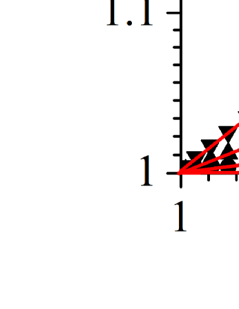
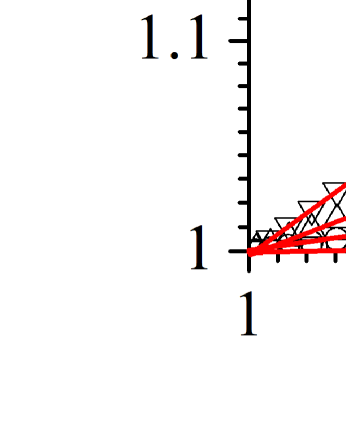
Figure 4: ($a$) $G(q)$ as functions of $G(-2)$ for $q=-1,-3,-5,-7$; ($b$) $G(q)$ as functions of $G(2)$ for $q=1,3,5,7$. Both vertical and horizontal axes in ($a$) and ($b$) are plotted in logarithmic form.

ESS (i.e., Eq. (6)) is another scaling predicted by the multifractal formalism. Different from SSS, ESS does not rely on the i.i.d of the addends, but the additive process (see Eq. (2)). Fig. 4($a$) and 4($b$) shows the ESS scalings for $q_{0}=-2$ and $q_{0}=2$, respectively. ESS holds for the entire logarithmic region. The observation suggests that the streamwise wall-shear fluctuations generated by logarithmic motions obey the additive process, though the streamwise wall shear fluctuations generated by attached eddies with wall-normal heights at approximately $0.2h^{+}$ are not identically and independently distributed due to the scale interactions (see Fig. 2), which are not described by the attached-eddy model.

4.2 Instantaneous distribution of $\tau^{\prime}_{x}$

Furthermore, the instantaneous $\tau_{x}^{{}^{\prime}+}$ can be decomposed as

$$\tau_{x}^{{}^{\prime}+}=\tau_{x,s}^{{}^{\prime}+}+\underbrace{\tau_{x,L}^{{}^{\prime}+}(y_{s}^{+})-\tau_{x,L}^{{}^{\prime}+}(y_{e}^{+})}_{\tau_{x,log}^{{}^{\prime}+}}+\underbrace{\tau_{x,L}^{{}^{\prime}+}(y_{e}^{+})}_{\tau_{x,out}^{{}^{\prime}+}},$$ (14)

where $\tau_{x,s}^{{}^{\prime}+}$ denotes the amplitude modulation of the universal signal $\tau_{x}^{{}^{\prime}*+}$, $\tau_{x,log}^{{}^{\prime}+}$ and $\tau_{x,out}^{{}^{\prime}+}$ are the superposition components contributed from the log region and the outer wall-coherent motions, respectively. The methodology of removing modulation effects can be found in Mathis et al. (2011) and Baars et al. (2016), whose details are out of the range of present study. Fig. 5($a$) shows the probability density functions (p.d.f.s) of $\tau_{x}^{{}^{\prime}*+}$, $\tau_{x,s}^{{}^{\prime}+}$, $\tau_{x,log}^{{}^{\prime}+}$ and $\tau_{x,out}^{{}^{\prime}+}$, and compares with the p.d.f for the full channel data. The p.d.f.s of $\tau_{x,s}^{{}^{\prime}+}$ and $\tau_{x}^{{}^{\prime}*+}$ nearly coincide with that of $\tau_{x}^{{}^{\prime}+}$ with asymmetric and positively skewed shape, which demonstrates that removing the superposition and modulation effects barely affects the instantaneous distributions. The asymmetries between the positive and negative wall-shear fluctuations are the essential characters of the near-wall small-scale turbulence, which may be associated with the celebrated near-wall sustaining process (Schoppa & Hussain, 2002). In contrast, the p.d.f.s of $\tau_{x,log}^{{}^{\prime}+}$ and $\tau_{x,out}^{{}^{\prime}+}$ are more symmetric with rare events invisible, suggesting that the superposition components of logarithmic and outer motions are less intermittent than the small-scale universal signals. This also explains the reason why the log-normal model describes the additive process well (see Fig. 3($a$)), although the log-normal model is inapplicable for rare events (Landau & Lifshitz, 1987). Moreover, the skewness and flatness of $\tau_{x,log}^{{}^{\prime}+}$ are 0.05 and 2.91, which are very close to those of a Gaussian distribution. It strongly supports the conclusion drawn above that the streamwise wall-shear stress fluctuations generated by attached eddies populating logarithmic region can be absolutely treated as Gaussian variables with

$$p(\xi)=\frac{1}{\sqrt{2\pi}\sigma}\exp\left(-\frac{\xi^{2}}{2\sigma^{2}}\right),$$ (15)

where $p(\xi)$ denotes the p.d.f, and $\xi$ is the independent variable. It is worth noting that the variation of variance can be well predicted by the log-normal model, namely

$$\sigma^{2}=\left.\frac{\partial^{2}G(q;y_{o}^{+})}{\partial q^{2}}\right|_{q=0}=2C_{2}\ln(Re_{\tau})+C_{3},$$ (16)

where $C_{2}\approx 0.00629$, and $C_{3}\approx-0.07959$ is a constant and determined by the DNS data at $Re_{\tau}=2003$. Fig. 5($b$) shows the p.d.f.s of $\tau_{x,log}^{{}^{\prime}+}$ and the model prediction by Eq. (15), results of other two Reynolds numbers (Del Álamo et al., 2004; Lozano-Durán & Jiménez, 2014) are also included for comparison. It can be seen that the Gaussian model proposed here works reasonably well and can cover a wide range of Reynolds numbers. The model remains to be validated by higher-Reynolds number DNS data.

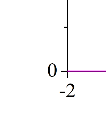
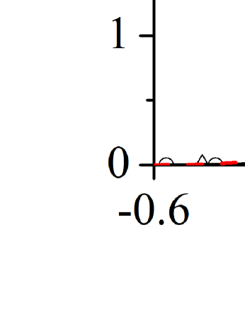
Figure 5: ($a$) P.d.f.s of $\tau_{x}^{{}^{\prime}*+}$, $\tau_{x,s}^{{}^{\prime}+}$, $\tau_{x,log}^{{}^{\prime}+}$, $\tau_{x,out}^{{}^{\prime}+}$, and $\tau_{x}^{{}^{\prime}+}$; ($b$) P.d.f.s of $\tau_{x,log}^{{}^{\prime}+}$ in channel flows with $Re_{\tau}=934$, $2003$, and $4179$. Dashed lines denote the Gaussian model predictions with Eqs. (15)-(16).

5 Concluding remarks

In summary, the present study reveals that IOIM and AEM are consistent to each other quantitatively. The statistical characteristics of the superpositions of log-region eddies follow the predictions of AEM, namely, the SSS and ESS scalings. Based on these observations, we conclude that the streamwise wall-shear stress fluctuations generated by attached eddies populating the logarithmic region can be treated as Gaussian variables. A Gaussian model is then proposed to describe their instantaneous distributions and verified by DNS data spanned broad-band Reynolds numbers. Considering the fact that the intensity of wall-shear stress fluctuations is typically underpredicted by the state-of-the-art wall-modelled large-eddy simulation (WMLES) approaches (Park & Moin, 2016), the Gaussian model proposed in the present study may be constructive for the development of the LES methodology, and the distribution characteristics of $\tau_{x}^{{}^{\prime}*+}$ are helpful for developing more accurate near-wall models of WMLES approaches.

It is noted that some previous works adopted IOIM to investigate the spectral characteristics of the wall-coherent components of the signals in near-wall region, such as the work of Marusic et al. (2017), but whether they are consistent with the AEM predictions in physical space quantitatively has not been verified in detail. The consistency of the two models demonstrated here fills the gap and complements their works. Moreover, the findings in present study indicate that we can isolate the footprints of attached eddies within a selected wall-normal range by employing IOIM, i.e., by adjusting $y_{1}^{+}$ and $y_{2}^{+}$ in $\tau_{x,L}^{{}^{\prime}+}(y_{1}^{+})-\tau_{x,L}^{{}^{\prime}+}(y_{2}^{+})$. Here $y_{1}^{+}$ and $y_{2}^{+}$ are two selected wall-normal heights in the logarithmic region, and $y_{1}^{+}<y_{2}^{+}$. In this regard, the present study may provide a new perspective for analyzing some flow physics in wall-bounded turbulence, such as the inner peak of the intensity of $u^{\prime}$, and the streamwise inclined angles of attached eddies. All these are under investigation currently and will be reported in separate forthcoming papers.

Declaration of interests

The authors report no conflict of interest.

References

- Abe et al. (2004) Abe, H., Kawamura, H. & Choi, H. 2004 Very large-scale structures and their effects on the wall shear-stress fluctuations in a turbulent channel flow up to . J. Fluids Eng. 126 (5), 835–843.
- Baars & Marusic (2020) Baars, W.J. & Marusic, I. 2020 Data-driven decomposition of the streamwise turbulence kinetic energy in boundary layers. part 1. energy spectra. J. Fluid Mech. 882.
- Baars et al. (2016) Baars, W. J, Hutchins, N. & Marusic, I. 2016 Spectral stochastic estimation of high-reynolds-number wall-bounded turbulence for a refined inner-outer interaction model. Physical Review Fluids 1 (5), 054406.
- Benzi et al. (1993) Benzi, R., Ciliberto, S., Tripiccione, R., Baudet, C., Massaioli, F. & Succi, S. 1993 Extended self-similarity in turbulent flows. Phys. Rev. E 48, R29–R32.
- Blackman et al. (2019) Blackman, K., Perret, L. & Mathis, R. 2019 Assessment of inner–outer interactions in the urban boundary layer using a predictive model. J. Fluid Mech. 875, 44–70.
- Cheng et al. (2019) Cheng, C., Li, W., Lozano-Durán, A. & Liu, H. 2019 Identity of attached eddies in turbulent channel flows with bidimensional empirical mode decomposition. J. Fluid Mech 870, 1037–1071.
- Cheng et al. (2020) Cheng, C., Li, W., Lozano-Durán, A. & Liu, H. 2020 On the structure of streamwise wall-shear stress fluctuations in turbulent channel flows. J. Fluid Mech. 903, A29.
- Del Álamo & Jiménez (2003) Del Álamo, J. C. & Jiménez, J. 2003 Spectra of the very large anisotropic scales in turbulent channels. Phys. Fluids 15 (6), L41–L44.
- Del Álamo et al. (2004) Del Álamo, J. C., Jiménez, J., Zandonade, P. & Moser, R.D. 2004 Scaling of the energy spectra of turbulent channels. J. Fluid Mech. 500, 135–144.
- Diaz-Daniel et al. (2017) Diaz-Daniel, C., Laizet, S. & Vassilicos, J.C. 2017 Wall shear stress fluctuations: Mixed scaling and their effects on velocity fluctuations in a turbulent boundary layer. Phys. Fluids 29 (5), 055102.
- Frisch & Donnelly (1996) Frisch, U. & Donnelly, R.J. 1996 Turbulence: the legacy of AN Kolmogorov. AIP.
- de Giovanetti et al. (2016) de Giovanetti, M., Hwang, Y. & Choi, H. 2016 Skin-friction generation by attached eddies in turbulent channel flow. J. Fluid Mech. 808, 511–538.
- Guerrero et al. (2020) Guerrero, B., Lambert, M.F. & Chin, R.C. 2020 Extreme wall shear stress events in turbulent pipe flows: spatial characteristics of coherent motions. J. Fluid Mech. 904, A18.
- Hoyas & Jiménez (2006) Hoyas, S. & Jiménez, J. 2006 Scaling of the velocity fluctuations in turbulent channels up to . Phys. Fluids 18 (1), 011702.
- Hu et al. (2006) Hu, Z.W., Morfey, C.L. & Sandham, N.D. 2006 Wall pressure and shear stress spectra from direct simulations of channel flow. AIAA Journal 44 (7), 1541–1549.
- Hwang (2015) Hwang, Y. 2015 Statistical structure of self-sustaining attached eddies in turbulent channel flow. J. Fluid Mech. 767, 254–289.
- Iwamoto et al. (2002) Iwamoto, K., Suzuki, Y. & Kasagi, N. 2002 Reynolds number effect on wall turbulence: toward effective feedback control. Int. J. Heat Fluid Flow 23 (5), 678–689.
- Jiménez (2018) Jiménez, J. 2018 Coherent structures in wall-bounded turbulence. J. Fluid Mech. 842, P1.
- Jiménez & Hoyas (2008) Jiménez, J. & Hoyas, S. 2008 Turbulent fluctuations above the buffer layer of wall-bounded flows. J. Fluid Mech. 611, 215–236.
- Kaneda & Yamamoto (2021) Kaneda, Y. & Yamamoto, Y. 2021 Velocity gradient statistics in turbulent shear flow: an extension of kolmogorov’s local equilibrium theory. J. Fluid Mech. 929, A13.
- Landau & Lifshitz (1987) Landau, L. & Lifshitz, E 1987 Fluid mechanics. In Course of Theoretical Physics, Pergamon.
- Lee & Moser (2015) Lee, M. & Moser, R.D. 2015 Direct numerical simulation of turbulent channel flow up to . J. Fluid Mech. 774, 395–415.
- Li et al. (2019) Li, W., Fan, Y., Modesti, D. & Cheng, C. 2019 Decomposition of the mean skin-friction drag in compressible turbulent channel flows. J. Fluid Mech. 875, 101–123.
- Lozano-Durán & Jiménez (2014) Lozano-Durán, A. & Jiménez, J. 2014 Time-resolved evolution of coherent structures in turbulent channels: characterization of eddies and cascades. J. Fluid Mech. 759, 432–471.
- Mandelbrot (1974) Mandelbrot, B.B 1974 Intermittent turbulence in self-similar cascades: divergence of high moments and dimension of the carrier. J. Fluid Mech. 62 (2), 331–358.
- Marusic et al. (2017) Marusic, I., Baars, W.J. & Hutchins, N. 2017 Scaling of the streamwise turbulence intensity in the context of inner-outer interactions in wall turbulence. Phys. Rev. Fluids 2 (10), 100502.
- Marusic et al. (2010) Marusic, I., Mathis, R. & Hutchins, N. 2010 Predictive model for wall-bounded turbulent flow. Science 329 (5988), 193–196.
- Marusic & Monty (2019) Marusic, I. & Monty, J.P. 2019 Attached eddy model of wall turbulence. Annu. Rev. Fluid Mech. 51, 49–74.
- Mathis et al. (2011) Mathis, R., Hutchins, N. & Marusic, I. 2011 A predictive inner–outer model for streamwise turbulence statistics in wall-bounded flows. J. Fluid Mech. 681, 537–566.
- Mathis et al. (2013) Mathis, R., Marusic, I., Chernyshenko, S.I. & Hutchins, N. 2013 Estimating wall-shear-stress fluctuations given an outer region input. J. Fluid Mech. 715, 163–180.
- Meneveau & Marusic (2013) Meneveau, C. & Marusic, I. 2013 Generalized logarithmic law for high-order moments in turbulent boundary layers. J. Fluid Mech. 719.
- Park & Moin (2016) Park, G.I. & Moin, P. 2016 Space-time characteristics of wall-pressure and wall shear-stress fluctuations in wall-modeled large eddy simulation. Phys. Rev. Fluids 1 (2), 024404.
- Perry & Chong (1982) Perry, A. E. & Chong, M. S 1982 On the mechanism of wall turbulence. J. Fluid Mech. 119 (119), 173–217.
- Schlatter & Örlü (2010) Schlatter, P. & Örlü, R. 2010 Assessment of direct numerical simulation data of turbulent boundary layers. J. Fluid Mech. 659, 116–126.
- Schoppa & Hussain (2002) Schoppa, W & Hussain, Fazle 2002 Coherent structure generation in near-wall turbulence. J. Fluid Mech. 453, 57–108.
- Townsend (1976) Townsend, A. A. 1976 The structure of turbulent shear flow, 2nd edn. Cambridge University Press.
- Wang et al. (2020) Wang, J., Pan, C. & Wang, J. 2020 Characteristics of fluctuating wall-shear stress in a turbulent boundary layer at low-to-moderate Reynolds number. Phys. Rev. Fluids 5 (7), 074605.
- Wang et al. (2021) Wang, L., Hu, R. & Zheng, X. 2021 A scaling improved inner–outer decomposition of near-wall turbulent motions. Physics of Fluids 33 (4), 045120.
- Yang & Lozano-Durán (2017) Yang, X.I.A. & Lozano-Durán, A. 2017 A multifractal model for the momentum transfer process in wall-bounded flows. J. Fluid Mech. 824, R2.
- Yang et al. (2016) Yang, X.I.A., Marusic, I. & Meneveau, C. 2016 Moment generating functions and scaling laws in the inertial layer of turbulent wall-bounded flows. J Fluid Mech 791, R2.