Factorial cumulants from short-range correlations and global baryon number conservation

Abstract

We calculate the baryon factorial cumulants assuming arbitrary short-range correlations and the global baryon number conservation. The general factorial cumulant generating function is derived. Various relations between factorial cumulants subjected to baryon number conservation and the factorial cumulants without this constraint are presented. We observe that for $n$-th factorial cumulant, the short-range correlations of more than $n$ particles are suppressed with the increasing number of particles. The recently published Vovchenko et al. (2020) relations between the cumulants in a finite acceptance with global baryon conservation and the grand-canonical susceptibilities are reproduced.

I Introduction

Search for the predicted first-order phase transition and the corresponding critical end point between the hadronic matter and quark-gluon plasma is one of the most important challenges in high-energy physics Stephanov (2004); Braun-Munzinger and Wambach (2009); Braun-Munzinger et al. (2016); Bzdak et al. (2020). Since fluctuations of such observables as baryon number, electric charge or strangeness number are sensitive to the phase transitions, they are broadly studied both theoretically and experimentally in relativistic heavy-ion collisions Jeon and Koch (2000); Asakawa et al. (2000); Gazdzicki et al. (2004); Gorenstein et al. (2004); Stephanov (2004); Koch et al. (2005); Stephanov (2009); Cheng et al. (2009); Fu et al. (2010); Skokov et al. (2011); Stephanov (2011); Karsch and Redlich (2011); Schaefer and Wagner (2012); Chen et al. (2011); Luo et al. (2012); Zhou et al. (2012); Wang and Yang (2012); Herold et al. (2016); Luo and Xu (2017); Szymański et al. (2020); Ratti (2019).

Higher-order cumulants, $\kappa_{n}$, are commonly used to describe such fluctuations Stephanov (2009); Behera (2019); Acharya et al. (2020); Skokov et al. (2012); Braun-Munzinger et al. (2012); Bzdak and Koch (2012); Braun-Munzinger et al. (2017); Adamczyk et al. (2018); Adare et al. (2016). Nevertheless, the cumulants mix the correlation functions of different orders and also they may be dominated by the trivial average number of particles. On the other hand, the factorial cumulants, $\hat{C}_{n}$, represent the integrated multiparticle correlation functions Botet and Ploszajczak (2002); Ling and Stephanov (2016); Bzdak et al. (2017a, 2020) and their applications can be seen, e.g., in Refs. Adamczyk et al. (2014); Bzdak et al. (2017a, 2018); Bzdak and Koch (2019); Adamczewski-Musch et al. (2020a); Abdallah et al. (2021); Vovchenko et al. (2022). However, one should be careful because various effects such as the impact parameter fluctuation or the conservation laws may be reflected in the anomalies of factorial cumulants or cumulants Skokov et al. (2013); Braun-Munzinger et al. (2017); Bzdak et al. (2017b); Adamczewski-Musch et al. (2020b); Kitazawa and Asakawa (2012); Bzdak et al. (2013); Braun-Munzinger et al. (2017); Rogly et al. (2019); Braun-Munzinger et al. (2019); Acharya et al. (2020); Savchuk et al. (2020); Braun-Munzinger et al. (2021); Vovchenko et al. (2022).

In our previous paper Barej and Bzdak (2020) we calculated the proton, antiproton and mixed proton-antiproton factorial cumulants assuming that the global baryon number conservation is the only source of correlations. We assumed that the acceptance is governed by the binomial distribution, which is correct if there are no other sources of correlations. Recently in Ref. Vovchenko et al. (2020), it was argued that applying the binomial acceptance is not correct if, e.g., short-range correlations are present in the system. Instead of the binomial acceptance, the subensemble acceptance method (SAM) was proposed. Using this approach, the relation between cumulants in a finite acceptance with global baryon conservation and the grand-canonical susceptibilities (cumulants), measured, e.g., on the lattice, was derived. The calculation presented in Vovchenko et al. (2020) assumes that the subvolume, in which cumulants are calculated, is large enough to be close to the thermodynamic limit.

In this paper we use SAM to study the factorial cumulants for one species of particles subjected to short-range correlations and the global baryon number conservation. In particular, we derive the general factorial cumulant generating function and various relations between factorial cumulants subjected to baryon number conservation and cumulants without this constraint. We also observe that for $n$-th factorial cumulant, the short-range correlations of more than $n$ particles are suppressed with the increasing total number of particles. Finally, we reproduce the main results of Ref. Vovchenko et al. (2020).

In the next Section, we present our derivation of the factorial cumulant generating function. In Section III we discuss in detail the case of two-particles short-range correlations, providing analytical formulas for the factorial cumulant generating function and the factorial cumulants up to the sixth order. We analyze their dependencies on the correlation strength and acceptance and propose certain approximations. Then, in Section IV, we move to multiparticle correlations. This is followed by the comparison of the cumulants obtained in our computation with the outcome of Ref. Vovchenko et al. (2020). Finally, we present our comments and summary.

II Factorial cumulant generating function

Consider a system of a fixed volume and some number of baryons of one species only, say protons. We divide it into two subsystems which can exchange particles, see Fig. 1.

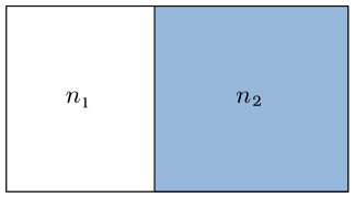
Figure 1: The system divided into two subsystems with $n_{1}$ particles in the first subvolume and $n_{2}$ particles in the second one. $n_{1}$ is inside and $n_{2}$ is outside of our acceptance.

Let $P_{1}(n_{1})$ be the probability that there are $n_{1}$ baryons in the first subsystem and $P_{2}(n_{2})$ be the probability that there are $n_{2}$ baryons in the second one. Then, the probability that there are $n_{1}$ particles in the first part and $n_{2}$ particles in the second one is given by

$$P(n_{1},n_{2})=P_{1}(n_{1})P_{2}(n_{2})\,,$$ (1)

if there are no correlations between the two subsystems. This equation is also approximately true for the case of short-range correlations, that is, if the correlation length is much shorter than the system size. In this paper we assume that this is exactly the case. We note that this is also one of the assumptions of the analysis of Ref. Vovchenko et al. (2020).

Now we impose the global baryon number conservation with a fixed total baryon number $B$. In this case

$$P_{B}(n_{1},n_{2})=A\;P_{1}(n_{1})P_{2}(n_{2})\delta_{n_{1}+n_{2},B}\,,$$ (2)

where $A$ is the normalization constant and $\delta_{n_{1}+n_{2},B}$ is the Kronecker delta responsible for the conservation law, that is $n_{1}+n_{2}=B$. The probability that there are $n_{1}$ particles in the first subvolume reads

$$P_{B}(n_{1})=\sum_{n_{2}=0}^{\infty}P_{B}(n_{1},n_{2})\,,$$ (3)

where the subscript $B$ indicates that the quantity is influenced by the conservation law.

The probability generating function corresponding to $P_{B}(n_{1})$ is

$$H_{(1,B)}(z)=\sum_{n_{1}=0}^{\infty}P_{B}(n_{1})z^{n_{1}}\,,$$ (4)

where here and in the following, the subscript $(1,B)$ indicates that the quantity from the first bin is influenced by the global baryon number conservation. Using the integral representation of the Kronecker delta:

$$\delta_{p,r}=\frac{1}{2\pi i}\oint_{|x|=1}\frac{dx}{x}x^{p-r}\,,$$ (5)

where $x$ is a complex variable, we obtain:

$$H_{(1,B)}(z)=\frac{A}{2\pi i}\oint_{|x|=1}\frac{dx}{x^{B+1}}H_{1}(xz)H_{2}(x)\,,$$ (6)

where

$$H_{i}(z)=\sum_{n_{i}=0}^{\infty}P_{i}(n_{i})z^{n_{i}}\,,\qquad i=1,2,$$ (7)

is the probability generating function for the multiplicity distribution $P_{i}(n_{i})$, $i=1,2$, free of the baryon number conservation.

The factorial cumulant generating function is given by (see, e.g., Bzdak et al. (2020)):

$$G(z)=\ln[H(z)]\,,$$ (8)

thus,

$$G_{(1,B)}(z)=\ln[H_{(1,B)}(z)]=\ln\left[\frac{A}{2\pi i}\oint_{|x|=1}\frac{dx}{x^{B+1}}\>e^{G_{1}(xz)}e^{G_{2}(x)}\right]\,,$$ (9)

where $G_{1}$ and $G_{2}$ are the factorial cumulant generating functions free of the baryon number conservation.

Using Cauchy’s differentiation formula:

$$\oint_{|x|=1}dx\frac{f(x)}{x^{B+1}}=\frac{2\pi i}{B!}\left.\frac{d^{B}f(x)}{dx^{B}}\right|_{x=0}\,,$$ (10)

we obtain

$$G_{(1,B)}(z)=\ln\left[\frac{A}{B!}\left.\frac{d^{B}}{dx^{B}}\left(e^{G_{1}(xz)}e^{G_{2}(x)}\right)\right|_{x=0}\right]\,.$$ (11)

We can express the factorial cumulant generating functions $G_{i}$ by the series of their factorial cumulants $\hat{C}_{k}^{(i)}$ ($i=1,2$ denoting the subvolume number). For example

$$G_{2}(x)=\sum_{k=1}^{\infty}\frac{(x-1)^{k}}{k!}\hat{C}_{k}^{(2)}\,.$$ (12)

This leads to

$$G_{(1,B)}(z)=\ln\left[\frac{A}{B!}\left.\frac{d^{B}}{dx^{B}}\exp\left(\sum_{k=1}^{\infty}\frac{(xz-1)^{k}\hat{C}_{k}^{(1)}+(x-1)^{k}\hat{C}_{k}^{(2)}}{k!}\right)\right|_{x=0}\right]\,.$$ (13)

Note that $\hat{C}_{k}^{(1)}$, $\hat{C}_{k}^{(2)}$ are respectively the factorial cumulants in the first and the second subsystems for the multiplicity distributions free of the global baryon conservation. As explained earlier, these factorial cumulants are sensitive to the short-range correlations only.

Finally, using the Faà di Bruno’s formula (for details see Appendix A) we obtain

$$G_{(1,B)}(z)=\ln\biggl{[}\frac{A^{\prime}}{B!}{\rm{Bell}}_{B}\biggl{(} \sum_{k=0}^{\infty}\frac{(-1)^{k}}{k!}\left[\hat{C}_{k+1}^{(1)}z+\hat{C}_{k+1}^{(2)}\right],$$ (14)

$$\sum_{k=0}^{\infty}\frac{(-1)^{k}}{k!}\left[\hat{C}_{k+2}^{(1)}z^{2}+\hat{C}_{k+2}^{(2)}\right],$$

$$\ldots,$$

$$\sum_{k=0}^{\infty}\frac{(-1)^{k}}{k!}\left[\hat{C}_{k+B}^{(1)}z^{B}+\hat{C}_{k+B}^{(2)}\right]\biggr{)}\biggr{]}\,,$$

where $A^{\prime}$ is a constant not relevant for further calculations, and ${\rm{Bell}}_{B}$ is the $B$-th complete exponential Bell polynomial:

$${\rm{Bell}}_{B}(x_{1},x_{2},...,x_{B})=\sum_{i=1}^{B}{\rm{Bell}}_{B,i}(x_{1},x_{2},...,x_{B-i+1})\,,$$ (15)

with ${\rm{Bell}}_{B,i}(x_{1},x_{2},...,x_{B-i+1})$ being the partial exponential Bell polynomials.

The goal of this paper is to relate the factorial cumulants $\hat{C}_{k}^{(1,B)}$ of $P_{B}(n_{1})$

$$\hat{C}_{k}^{(1,B)}=\left.\frac{d^{k}}{dz^{k}}G_{(1,B)}(z)\right|_{z=1}\,,$$ (16)

through the factorial cumulants $\hat{C}_{k}^{(1)}$, $\hat{C}_{k}^{(2)}$ of the probability distributions $P_{1}(n_{1})$ and $P_{2}(n_{2})$, respectively.

In this paper we allow for the short-range correlations only (besides the global baryon conservation which results in the long-range correlation) and consequently the factorial cumulants $\hat{C}_{k}^{(i)}$ (without baryon number conservation) of any order $k$ are proportional to the mean number of particles, see, e.g., Bzdak et al. (2020). We have

$$\hat{C}_{k}^{(1)} =\langle n_{1}\rangle\alpha_{k}=f\langle N\rangle\alpha_{k}\,,$$ (17)

$$\hat{C}_{k}^{(2)} =\langle n_{2}\rangle\alpha_{k}=(1-f)\langle N\rangle\alpha_{k}\,,$$

where $\langle N\rangle=\langle n_{1}\rangle+\langle n_{2}\rangle$ is the mean total number of particles in the system, $f$ is a fraction of particles in the first subvolume, and $\alpha_{k}$ describes the strength of $k$-particle short-range correlation ($\alpha_{1}=1$). If there are no short-range correlations in the system, then $\alpha_{k}=0$ for $k>1$. We note that $\langle n_{1}\rangle$ is the mean number of particles of $P_{1}(n_{1})$, that is, the distribution not affected by the global baryon conservation (and analogously for $\langle n_{2}\rangle$).

In the following we will usually assume that $\langle N\rangle=B$. Introducing the global baryon number conservation further requires that the total number of particles in every event equals $B$. That is why, the average number of baryons with the baryon number conservation included also equals $B$.

III Two-particle correlations

Here we consider two-particle short-range correlations only, that is, $\alpha_{2}\neq 0$ and $\alpha_{k}=0$ for $k\geq 3$.

III.1 An analytic approach using the Faà di Bruno’s formula and Bell polynomials

Applying Eqs. (17) to Eq. (14) with $\alpha_{k}=0$ for $k\geq 3$, we see that only the first two arguments of the $B$-th complete exponential Bell polynomial ${\rm{Bell}}_{B}$ are non-zero, that is

$$G_{(1,B)}(z)=\ln\biggl{[}\frac{A^{\prime}}{B!}{\rm{Bell}}_{B}\biggl{(}\sum_{k=0}^{1}\frac{(-1)^{k}}{k!}\langle N\rangle\alpha_{k+1}\left(f\ z+\bar{f}\,\right),\;\;\langle N\rangle\alpha_{2}\left(fz^{2}+\bar{f}\,\right),\;\;\underbrace{0,0,\ldots,0}_{(B-2)\text{ zeros}}\biggr{)}\biggr{]}\,,$$ (18)

where $\bar{f}=1-f$.

Using Eq. (15) we can rewrite it as follows

$$G_{(1,B)}(z)=\ln\biggl{\{}\frac{A^{\prime}}{B!} \biggl{[}{\rm{Bell}}_{B,B}\left((fz+\bar{f})\langle N\rangle(1-\alpha_{2})\right)$$ (19)

$$+\sum_{i=1}^{B-1}{\rm{Bell}}_{B,i}\biggl{(}(fz+\bar{f}\,)\langle N\rangle(1-\alpha_{2}),\;\;(fz^{2}+\bar{f}\,)\langle N\rangle\alpha_{2},\;\underbrace{0,0,\ldots,0}_{(B-i-1)\text{ zeros}}\biggr{)}\biggr{]}\biggr{\}}\,.$$

In the next step we apply the definition of the partial exponential Bell polynomials:

$${\rm{Bell}}_{B,i}(x_{1},x_{2},...,x_{B-i+1})=\sum\frac{B!}{j_{1}!j_{2}!\cdots j_{B-i+1}!}\left(\frac{x_{1}}{1!}\right)^{j_{1}}\left(\frac{x_{2}}{2!}\right)^{j_{2}}\cdots\left(\frac{x_{B-i+1}}{(B-i+1)!}\right)^{j_{B-i+1}}\,,$$ (20)

where the sum is over the non-negative integer $j_{1},j_{2},...,j_{B-i+1}$ such that

$$j_{1}+j_{2}+...+j_{B-i+1}=i\,,$$ (21)

$$j_{1}+2j_{2}+3j_{3}+...+(B-i+1)j_{B-i+1}=B\,.$$

However in our case: $x_{3}=x_{4}=...=x_{B-i+1}=0$, so we have non-zero terms in Eq. (20) if and only if $j_{3}=j_{4}=...=j_{B-i+1}=0$ (because $0^{r}\neq 0$ for $r=0$ only). In this case, the constraints (21) lead to $j_{1}=2i-B$, $j_{2}=B-i$. Since both $j_{1}$ and $j_{2}$ have to be greater than or equal to 0, meaning $B/2\leq i\leq B$, we obtain

$$G_{(1,B)}(z)=\ln\biggl{[}\frac{A^{\prime}}{B!}\sum_{i=B_{0}}^{B}\frac{B!}{(2i-B)!(B-i)!}\;\left[(fz+\bar{f}\,)\langle N\rangle(1-\alpha_{2})\right]^{2i-B}\left[\tfrac{1}{2}(fz^{2}+\bar{f}\,)\langle N\rangle\alpha_{2}\right]^{B-i}\biggr{]}\,,$$ (22)

where

$$B_{0}=\left\lceil\frac{B}{2}\right\rceil\equiv\begin{cases}\frac{B}{2},&\text{for }B\text{ even}\\ \frac{B+1}{2},&\text{for }B\text{ odd}\end{cases}\,.$$ (23)

Taking $\langle N\rangle=B$ we can rewrite $G_{(1,B)}(z)$ as

$$G_{(1,B)}(z)=\ln\biggl{[} A^{\prime}\frac{[B(1-\alpha_{2})(fz+\bar{f})]^{2B_{0}-B}\left[\frac{1}{2}B\alpha_{2}(fz^{2}+\bar{f})\right]^{B-B_{0}}}{(B-B_{0})!}$$ (24)

$$\times{}_{2}F_{2}\left(1,B_{0}-B;B_{0}-\frac{B}{2}+\frac{1}{2},B_{0}-\frac{B}{2}+1;-\frac{B(1-\alpha_{2})^{2}(fz+\bar{f})^{2}}{2\alpha_{2}(fz^{2}+\bar{f})}\right)\biggr{]}\,,$$

where ${}_{2}F_{2}(...)$ is the generalized hypergeometric function defined as

$${}_{2}F_{2}(a_{1},a_{2};b_{1},b_{2};z)=\sum_{n=0}^{\infty}\frac{(a_{1})^{(n)}(a_{2})^{(n)}}{(b_{1})^{(n)}(b_{2})^{(n)}}\frac{z^{n}}{n!}$$ (25)

with

$$(x)^{(n)}=\begin{cases}\prod_{k=0}^{n-1}(x+k),&\text{if $n=1,2,3,...$ }\\ 1,&\text{if $n=0$}\end{cases}$$ (26)

being the rising factorial (Pochhammer symbol).

Note that for even $B$, the fourth argument of ${}_{2}F_{2}$ becomes 1 whereas for odd $B$ the third argument becomes 1. Therefore, ${}_{2}F_{2}$ is in either case reduced to ${}_{1}F_{1}$ (the confluent hypergeometric function). Moreover, $(B_{0}-B)$, the second argument of ${}_{2}F_{2}$ is a negative integer, so $(B_{0}-B)^{(n)}=0$ starting from $n=B-B_{0}+1$. Therefore, the sum in ${}_{2}F_{2}$ is in fact finite from $n=0$ to $B-B_{0}$.

The factorial cumulants obtained from Eq. (24), see Eq. (16), read:

$$\hat{C}_{1}^{(1,B)} =fB\,,$$ (27)

$$\hat{C}_{2}^{(1,B)} =-f^{2}B+2f\beta-\frac{f\beta\gamma}{\alpha_{2}}R_{1}\,,$$ (28)

$$\hat{C}_{3}^{(1,B)} =2f^{3}B-12f^{2}\beta+6\frac{f^{2}\beta\gamma}{\alpha_{2}}R_{1}\,,$$ (29)

$$\hat{C}_{4}^{(1,B)} =-3!f^{4}B-12f^{2}(1-7f)\beta-3\frac{f^{2}\beta\gamma}{\alpha_{2}^{2}}\left[\beta\gamma R_{1}^{2}-4(1-4f)\alpha_{2}R_{1}-2\bar{f}\gamma(B-B_{0}-1)R_{2}\right]$$ (30)

$$\hat{C}_{5}^{(1,B)} =4!f^{5}B+240f^{3}(1-3f)\beta+60\frac{f^{3}\beta\gamma}{\alpha_{2}^{2}}\left[\beta\gamma R_{1}^{2}-4(1-2f)\alpha_{2}R_{1}-2\bar{f}\gamma(B-B_{0}-1)R_{2}\right]$$ (31)

$$\hat{C}_{6}^{(1,B)} =-5!f^{6}B+60\frac{f^{3}\beta}{\alpha_{2}}\left[-\bar{f}^{2}\gamma+4(31f^{2}-17f+1)\alpha_{2}\right]$$ (32)

$$-15\frac{f^{3}\beta\gamma}{\alpha_{2}^{3}}\biggl{[}2\beta^{2}\gamma^{2}R_{1}^{3}-6\bar{f}\beta\gamma^{2}(B-B_{0}-1)R_{1}R_{2}-12\beta\gamma(1-6f)\alpha_{2}R_{1}^{2}$$

$$\phantom{-15\frac{f^{3}\gamma}{\alpha_{2}^{3}}\biggl{[}}+2\alpha_{2}^{2}\left[191f^{2}-142f+11-B_{0}(3+2B_{0})\bar{f}^{2}\right]R_{1}$$

$$\phantom{-15\frac{f^{3}\gamma}{\alpha_{2}^{3}}\biggl{[}}+\alpha_{2}\bar{f}^{2}B\left[(2\alpha_{2}^{2}-5\alpha_{2}+2)B-2(\alpha_{2}^{2}-4\alpha_{2}+1)B_{0}-(4\alpha_{2}^{2}-11\alpha_{2}+4)\right]R_{1}$$

$$\phantom{-15\frac{f^{3}\gamma}{\alpha_{2}^{3}}\biggl{[}}+2\bar{f}\gamma(B-B_{0}-1)\left[(7-4B_{0}\bar{f}-67f)\alpha_{2}-B\bar{f}(1-4\alpha_{2}+\alpha_{2}^{2})\right]R_{2}\biggr{]}\,,$$

where the commonly appearing terms are defined as follows:

$$\beta=(B-B_{0})\bar{f}\,,$$ (33)

$$\gamma=B(1-\alpha_{2})^{2}\,,$$ (34)

$$R_{n}=\frac{{{}_{2}\widetilde{F}_{2}}\left(1+n,B_{0}-B+n;B_{0}-\frac{B}{2}+\frac{1}{2}+n,B_{0}-\frac{B}{2}+1+n;-\frac{B(1-\alpha_{2})^{2}}{2\alpha_{2}}\right)}{{{}_{2}\widetilde{F}_{2}}\left(1,B_{0}-B;B_{0}-\frac{B}{2}+\frac{1}{2},B_{0}-\frac{B}{2}+1;-\frac{B(1-\alpha_{2})^{2}}{2\alpha_{2}}\right)}\,,$$ (35)

whith

$${{}_{2}\widetilde{F}_{2}}(a_{1},a_{2};b_{1},b_{2},z)=\frac{{}_{2}F_{2}(a_{1},a_{2};b_{1},b_{2},z)}{\Gamma(b_{1})\Gamma(b_{2})}\,$$ (36)

being the regularized generalized hypergeometric function.

III.2 An approximate approach using general Leibnitz formula

In the case of two-particle correlations only, Eq. (13) reads:

$$G_{(1,B)}(z)=\ln\biggl{[}\frac{A}{B!}\biggl{.}\frac{d^{B}}{dx^{B}} \biggl{[}\exp\biggl{(}(xz-1)f\langle N\rangle+(x-1)\bar{f}\langle N\rangle\biggr{)}\times$$ (37)

$$\,\,\exp\biggl{(}\frac{1}{2}(xz-1)^{2}f\langle N\rangle\alpha_{2}+\frac{1}{2}(x-1)^{2}\bar{f}\langle N\rangle\alpha_{2}\biggr{)}\biggr{]}\biggr{|}_{x=0}\biggr{]}\,,$$

where $\alpha_{2}$ is defined in Eq. (17).

Assuming $\alpha_{2}$ to be small, we can expand the second exponent in Eq. (37) into a series. Then, we calculate the $B$-th derivative of a product of two functions, which is given by the general Leibnitz formula:

$$\frac{d^{B}(u\,v)}{dx^{B}}=\sum_{k=0}^{B}\binom{B}{k}\frac{d^{B-k}u}{dx^{B-k}}\frac{d^{k}v}{dx^{k}}\,.$$ (38)

In our case:

$$u(x)=\exp\left((xz-1)f\langle N\rangle+(x-1)\bar{f}\langle N\rangle\right)\,,$$ (39)

$$v(x) =\exp\left(\tfrac{1}{2}(xz-1)^{2}f\langle N\rangle\alpha_{2}+\tfrac{1}{2}(x-1)^{2}\bar{f}\langle N\rangle\alpha_{2}\right)$$ (40)

$$\approx\sum_{m=0}^{m_{max}}\frac{1}{m!}\left(\tfrac{1}{2}(xz-1)^{2}f\langle N\rangle\alpha_{2}+\tfrac{1}{2}(x-1)^{2}\bar{f}\langle N\rangle\alpha_{2}\right)^{m}\,,$$

$$\frac{d^{k}u}{dx^{k}}=\left(\bar{f}\langle N\rangle+f\,z\langle N\rangle\right)^{k}\exp\left((xz-1)f\langle N\rangle+(x-1)\bar{f}\langle N\rangle\right)\,,$$ (41)

$$\frac{d^{k}v}{dx^{k}}=0\qquad\text{for }k>2m_{max}\,.$$ (42)

Taking $\langle N\rangle=B$ we obtain:

$$G_{(1,B)}(z) =\ln(A)-\ln(B!)-B+B\ln(BY_{1})$$ (43)

$$+\ln\biggl{[}1$$

$$\phantom{+\ln}+\tfrac{1}{2}B\biggl{(}\frac{B-1}{B}X_{2}-1\biggr{)}\;\alpha_{2}$$

$$\phantom{+\ln}+\tfrac{1}{4!!}B^{2}\biggl{(}\frac{B!}{(B-4)!}\frac{X_{2}^{2}}{B^{4}}-4\frac{B!}{(B-3)!}\frac{X_{2}}{B^{3}}+2\frac{B!}{(B-2)!}\frac{X_{2}+2}{B^{2}}-3\biggr{)}\;\alpha_{2}^{2}$$

$$\phantom{+\ln}+\tfrac{1}{6!!}B^{3}\biggl{(}\frac{B!}{(B-6)!}\frac{X_{2}^{3}}{B^{6}}-6\frac{B!}{(B-5)!}\frac{X_{2}^{2}}{B^{5}}+3\frac{B!}{(B-4)!}\frac{X_{2}(X_{2}+4)}{B^{4}}$$

$$\phantom{+\ln+\tfrac{1}{48}\langle N\rangle^{3}}-4\frac{B!}{(B-3)!}\frac{3X_{2}+2}{B^{3}}+3\frac{B!}{(B-2)!}\frac{X_{2}+4}{B^{2}}-5\biggr{)}\;\alpha_{2}^{3}$$

$$\phantom{+\ln}+\tfrac{1}{8!!}B^{4}\biggl{(}\frac{B!}{(B-8)!}\frac{X_{2}^{4}}{B^{8}}-8\frac{B!}{(B-7)!}\frac{X_{2}^{3}}{B^{7}}+4\frac{B!}{(B-6)!}\frac{X_{2}^{2}(X_{2}+6)}{B^{6}}-8\frac{B!}{(B-5)!}\frac{X_{2}(3X_{2}+4)}{B^{5}}$$

$$\phantom{+\ln+\tfrac{1}{48}\langle N\rangle^{3}}+2\frac{B!}{(B-4)!}\frac{3X_{2}(X_{2}+8)+8}{B^{4}}-8\frac{B!}{(B-3)!}\frac{3X_{2}+4}{B^{3}}+4\frac{B!}{(B-2)!}\frac{X_{2}+6}{B^{2}}-7\biggr{)}\;\alpha_{2}^{4}$$

$$\phantom{+\ln}+\ldots\biggr{]}\,,$$

where $X_{k}=Y_{k}/(Y_{1})^{k}$ and $Y_{k}=fz^{k}+\bar{f}$ (in this formula only $X_{2}$ and $Y_{1}$ appear).

Note that for large $B$ and very small $\alpha_{2}$ we obtain a simple formula:

$$G_{(1,B)}(z)\approx\ln(A)-\ln(B!)-B+B\ln(BY_{1})+\tfrac{1}{2}(X_{2}-1)B\;\alpha_{2}\,.$$ (44)

Using Eq. (16) we calculate $\hat{C}_{n}^{(1,B)}$ and again expand into the Taylor series in $\alpha_{2}$. We obtain:

$$\hat{C}_{1}^{(1,B)} =fB\,,$$ (45)

$$\hat{C}_{2}^{(1,B)} =-f^{2}B+\bar{f}f(B-1)\;\alpha_{2}+3\bar{f}f\frac{B-1}{B}\;\alpha_{2}^{2}-5\bar{f}f\frac{(B-1)(B-3)}{B^{2}}\;\alpha_{2}^{3}$$ (46)

$$+\bar{f}f\frac{(B-1)(7B^{2}-65B+105)}{B^{3}}\;\alpha_{2}^{4}+\ldots\,,$$

$$\hat{C}_{3}^{(1,B)} =2f^{3}B-6\bar{f}f^{2}(B-1)\;\alpha_{2}-18\bar{f}f^{2}\frac{B-1}{B}\;\alpha_{2}^{2}+30\bar{f}f^{2}\frac{(B-1)(B-3)}{B^{2}}\;\alpha_{2}^{3}$$ (47)

$$-6\bar{f}f^{2}\frac{(B-1)(7B^{2}-65B+105)}{B^{3}}\;\alpha_{2}^{4}+\ldots\,,$$

$$\hat{C}_{4}^{(1,B)} =-3!f^{4}B+36\bar{f}f^{3}(B-1)\;\alpha_{2}-6\bar{f}f^{2}(B-1)\frac{2\bar{f}B-15f-3}{B}\;\alpha_{2}^{2}$$ (48)

$$+12\bar{f}f^{2}(B-1)\frac{\bar{f}B^{2}-B(4f+11)+15(1+2f)}{B^{2}}\;\alpha_{2}^{3}$$

$$-6\bar{f}f^{2}(B-1)\frac{2\bar{f}B^{3}-21B^{2}(3-f)+15B(19+7f)-315(1+f)}{B^{3}}\;\alpha_{2}^{4}+\ldots\,,$$

$$\hat{C}_{5}^{(1,B)} =4!f^{5}B-240\bar{f}f^{4}(B-1)\;\alpha_{2}+120\bar{f}f^{3}(B-1)\frac{2\bar{f}B-3f-3}{B}\;\alpha_{2}^{2}$$ (49)

$$-240\bar{f}f^{3}(B-1)\frac{\bar{f}B^{2}-B(11-6f)+15}{B^{2}}\;\alpha_{2}^{3}$$

$$+120\bar{f}f^{3}(B-1)\frac{2\bar{f}B^{3}-7B^{2}(9-7f)+5B(57-31f)-105(3-f)}{B^{3}}\;\alpha_{2}^{4}+\ldots\,,$$

$$\hat{C}_{6}^{(1,B)} =-5!f^{6}B+1800\bar{f}f^{5}(B-1)\;\alpha_{2}-1800\bar{f}f^{4}(B-1)\frac{2\bar{f}B-3}{B}\;\alpha_{2}^{2}$$ (50)

$$-120\bar{f}f^{3}(B-1)\frac{-5\bar{f}(5f+1)B^{2}+(-238f^{2}+296f+17)B+15(14f^{2}-28f-1)}{B^{2}}\;\alpha_{2}^{3}$$

$$-360\bar{f}f^{3}(B-1)$$

$$\times\frac{2\bar{f}(2+3f)B^{3}+5B^{2}(47f^{2}-45f-9)-25B(39f^{2}-47f-5)+105(9f^{2}-13f-1)}{B^{3}}\;\alpha_{2}^{4}+\ldots\,.$$

Here we expand up to $\alpha_{2}^{4}$ but higher orders can be easily obtained.

We note that using Eq. (44) we simply obtain the first two terms in each $\hat{C}_{k}^{(1,B)}$ of Equations 45–50 (with $B-1\approx B$).

Having factorial cumulants, one can easily calculate cumulants $\kappa_{n}$. For example:

$$\kappa_{1}^{(1,B)} =fB\,,$$ (51)

$$\kappa_{2}^{(1,B)} =\bar{f}f\biggl{[}B+(B-1)\;\alpha_{2}+3\frac{B-1}{B}\;\alpha_{2}^{2}-5\frac{(B-1)(B-3)}{B^{2}}\;\alpha_{2}^{3}$$ (52)

$$\phantom{=f\bar{f}}\>+\frac{(B-1)(7B^{2}-65B+105)}{B^{3}}\;\alpha_{2}^{4}+\ldots\biggr{]}\,,$$

$$\kappa_{3}^{(1,B)} =\bar{f}f(1-2f)\biggl{[}B+3(B-1)\;\alpha_{2}+9\frac{B-1}{B}\;\alpha_{2}^{2}-15\frac{(B-1)(B-3)}{B^{2}}\;\alpha_{2}^{3}$$ (53)

$$\phantom{=\bar{f}f(1-2f)}\>+3\frac{(B-1)(7B^{2}-65B+105)}{B^{3}}\;\alpha_{2}^{4}+\ldots\biggr{]}\,,$$

$$\kappa_{4}^{(1,B)} =\bar{f}f\biggl{[}B(1-6\bar{f}f)+(B-1)[7-36\bar{f}f]\alpha_{2}+3\frac{B-1}{B}[7-2\bar{f}f(2B+15)]\alpha_{2}^{2}$$ (54)

$$\phantom{=\bar{f}f}\>-\frac{B-1}{B^{2}}[35(B-3)-12\bar{f}f(B^{2}+4B-30)]\alpha_{2}^{3}$$

$$\phantom{=\bar{f}f}\>+\frac{B-1}{B^{3}}[7(7B^{2}-65B+105)-6\bar{f}f(2B^{3}-21(B^{2}+5B-15))]\alpha_{2}^{4}+\ldots\biggr{]}\,.$$

III.3 Examples

To illustrate our results, in Fig. 2 we plot the factorial cumulants for $B=300$ and $f=0.2$ as a function of $\alpha_{2}$. We verified that the analytic results obtained using the Faà di Bruno’s formula and Bell polynomials, Eqs. (27)-(32), are equivalent to the exact computation obtained with differentiating Eq. (37) $B=300$ times. We compared them with approximate results obtained using general Leibnitz formula, Eqs. (45)-(50). As seen in Fig. 2, $\hat{C}_{2}^{(1,B)}$ and $\hat{C}_{3}^{(1,B)}$ are very well approximated already by a linear expansion in $\alpha_{2}$. This is not surprising. It is clear from Eqs. (46) and (47) that higher powers of $\alpha_{2}$ are suppressed for large $B$. Quartic expansions of $\hat{C}_{4}^{(1,B)}$ and $\hat{C}_{5}^{(1,B)}$ are in good agreement with exact results in the whole investigated range $-0.5\leq\alpha_{2}\leq 0.5$, whereas quartic expansion of $\hat{C}_{6}^{(1,B)}$ works in a narrower range of $-0.3\lesssim\alpha_{2}\lesssim 0.3$, which is acceptable since $\alpha_{2}$ was assumed to be rather small.

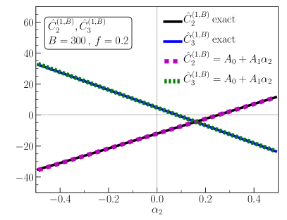
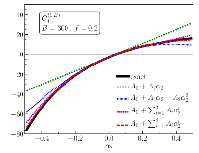
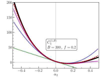
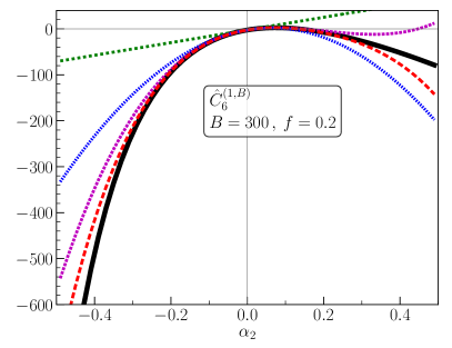
Figure 2: Factorial cumulants $\hat{C}_{n}^{(1,B)}$ ($n=2,3,...,6$, assuming $B=300$, $f=0.2$, and $\alpha_{k}=0$ for $k\geq 3$) as a function of the two-particle correlation strength, $\alpha_{2}$. The “exact” line in each plot represents the analytic result, Eqs. (27)-(32). Other lines represent approximate power series expansions, Eqs. (45)-(50). For $\hat{C}_{2}^{(1,B)}$ and $\hat{C}_{3}^{(1,B)}$ only linear terms are presented because higher powers of $\alpha_{2}$ give practically identical results.

It is also useful to plot these factorial cumulants as functions of $f$ for fixed $B$ and $\alpha_{2}$ (we choose $B=300$ and $\alpha_{2}=0.25$), see Fig. 3. For $\hat{C}_{2}^{(1,B)}$, $\hat{C}_{3}^{(1,B)}$, and $\hat{C}_{4}^{(1,B)}$ already a linear expansion in $\alpha_{2}$ is in good agreement with the exact results. In the case of $\hat{C}_{5}^{(1,B)}$ and $\hat{C}_{6}^{(1,B)}$ significant deviations between the linear $\alpha_{2}$ expansion and the exact function are observed. Including higher order terms up to $\alpha_{2}^{4}$ is sufficient to reproduce the exact results.

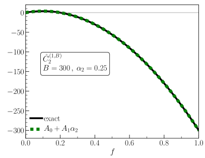
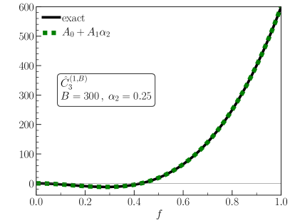
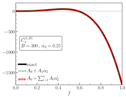
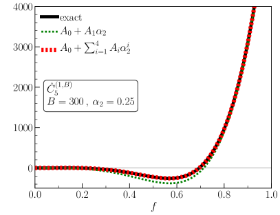
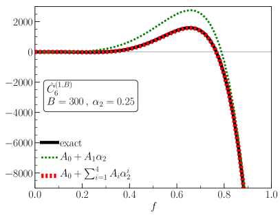
Figure 3: Factorial cumulants $\hat{C}_{n}^{(1,B)}$ ($n=2,3,...,6$, assuming $B=300$, $\alpha_{2}=0.25$, and $\alpha_{k}=0$ for $k\geq 3$) as a function of a fraction of particles in the first of the two subsystems, $f$. In each figure we show the “exact” line representing analytic results, Eqs. (27)-(32), and approximate expansions from Eqs. (45)-(50). For readability, we present only linear and quartic functions.

IV Multiparticle correlations

In this section we calculate the factorial cumulants taking into account the multiparticle short-range correlations. The generating function, Eq. (13), can be written as:

$$G_{(1,B)}(z)=\ln\biggl{[}\frac{A}{B!}\biggl{.}\frac{d^{B}}{dx^{B}} \biggl{[}\exp\left((xz-1)f\langle N\rangle+(x-1)\bar{f}\langle N\rangle\right)\left(\sum_{m=0}^{\infty}\frac{V^{m}}{m!}\right)\biggr{]}\biggr{|}_{x=0}\biggr{]}\,,$$ (55)

where

$$V=\sum_{k=2}^{5}\left(\frac{(xz-1)^{k}}{k!}f\langle N\rangle\alpha_{k}+\frac{(x-1)^{k}}{k!}\bar{f}\langle N\rangle\alpha_{k}\right)\,.$$ (56)

Here we assumed that $\alpha_{k}\neq 0$ for $k\leq 5$.

Considering $\alpha_{k}$ to be small we can limit our expansion to a linear term in $V$:

$$G_{(1,B)}(z)\approx\ln\biggl{[}\frac{A}{B!}\biggl{.}\frac{d^{B}}{dx^{B}}\biggl{[}\exp\left((xz-1)f\langle N\rangle+(x-1)\bar{f}\langle N\rangle\right)\left(1+V\right)\biggr{]}\biggr{|}_{x=0}\biggr{]}\,.$$ (57)

By evaluating the derivatives using the general Leibnitz formula, we obtain:

$$G_{(1,B)}(z)\approx\ln(A)-\ln(B!)-\langle N\rangle+B\ln(\langle N\rangle Y_{1})+\ln\biggl{[}1+\langle N\rangle\sum_{k=2}^{5}A_{k}\alpha_{k}\biggr{]}\,,$$ (58)

where

$$A_{k}=\frac{1}{k!}\sum_{j=0}^{k}(-1)^{k-j}\binom{k}{j}\frac{B!}{(B-j)!}\frac{X_{j}}{\langle N\rangle^{j}}\,,$$ (59)

and $X_{j}$, $Y_{1}$ are defined below Eq. (43).

The factorial cumulants are given by (here $\langle N\rangle=B$ and the calculated factorial cumulants are expanded in small $\alpha_{k}$)

$$\begin{aligned} \hat{C}_{1}^{(1,B)}=fB\,,\end{aligned}$$ (60)

$$\begin{aligned} \hat{C}_{2}^{(1,B)}&=-f^{2}B+\bar{f}f(B-1)\biggl{[}\;\alpha_{2}-2\frac{1}{B}\;\alpha_{3}-\frac{1}{2}\frac{B-6}{B^{2}}\;\alpha_{4}+\frac{4}{3}\frac{B-3}{B^{3}}\;\alpha_{5}\biggr{]}+\ldots\,,\end{aligned}$$ (61)

$$\begin{aligned} \hat{C}_{3}^{(1,B)}&=2f^{3}B-\bar{f}f(B-1)\biggl{[}6f\;\alpha_{2}+\frac{(2f-1)B+2(1-8f)}{B}\;\alpha_{3}-3\frac{(3f-1)B+2(1-5f)}{B^{2}}\alpha_{4}\\ &\phantom{2f^{3}B-\bar{f}f\frac{B-1}{B^{2}}[++}\;+\frac{1}{2}\frac{(1-2f)B^{2}+2(22f-7)B+24(1-4f)}{B^{3}}\alpha_{5}\biggr{]}+\ldots\,,\end{aligned}$$ (62)

$$\begin{aligned} \hat{C}_{4}^{(1,B)}&=-6f^{4}B+\bar{f}f(B-1)\biggl{[}36f^{2}\;\alpha_{2}+12f\frac{(2f-1)B+2(1-5f)}{B}\;\alpha_{3}\\ &\phantom{2f^{3}B-\bar{f}f\frac{B-1}{B^{2}}[}\;+\frac{B^{2}(3f^{2}-3f+1)-B(105f^{2}-51f+5)+6(45f^{2}-15f+1)}{B^{2}}\;\alpha_{4}\\ &\phantom{2f^{3}B-\bar{f}f\frac{B-1}{B^{2}}}\;-2\frac{B^{2}(12f^{2}-9f+2)-2B(69f^{2}-36f+5)+12(21f^{2}-9f+1)}{B^{3}}\;\alpha_{5}\biggr{]}+\ldots\,,\end{aligned}$$ (63)

Note that the $\alpha_{2}$ terms are in agreement with the linear part of Eqs. (45)-(48). The higher order factorial cumulants can be also readily derived.

In the limit of large $B$ (and small $\alpha_{k}$) the factorial cumulants read:

$$\hat{C}_{1}^{(1,B)} =fB\,,$$ (64)

$$\hat{C}_{2}^{(1,B)} \approx fB\left[-f+\bar{f}\alpha_{2}\right]\,,$$ (65)

$$\hat{C}_{3}^{(1,B)} \approx fB\left[2f^{2}-6\bar{f}f\alpha_{2}+\bar{f}(1-2f)\alpha_{3}\right]\,,$$ (66)

$$\hat{C}_{4}^{(1,B)} \approx fB\;[-3!f^{3}+36\bar{f}f^{2}\alpha_{2}-12\bar{f}f(1-2f)\alpha_{3}+\bar{f}(1-3\bar{f}f)\alpha_{4}]\,,$$ (67)

$$\hat{C}_{5}^{(1,B)}\approx fB[4!f^{4}-240f^{3}\bar{f}\alpha_{2}+120f^{2}\bar{f}(1-2f)\alpha_{3}-20f\bar{f}(1-3f\bar{f})\alpha_{4}$$ (68)

$$\phantom{fB[}+\bar{f}(1-2f)(1-2f\bar{f})\alpha_{5}]\,,$$

$$\hat{C}_{6}^{(1,B)}\approx fB[-5!f^{5}+1800f^{4}\bar{f}\alpha_{2}-1200f^{3}\bar{f}(1-2f)\alpha_{3}+300f^{2}\bar{f}(1-3f\bar{f})\alpha_{4}$$ (69)

$$\phantom{fB[}-30f\bar{f}(1-2f)(1-2f\bar{f})\alpha_{5}+\bar{f}(1-5f\bar{f}(1-f\bar{f}))\alpha_{6}]\,.$$

One can observe that for large $B$, $\hat{C}_{n}^{(1,B)}$ is not influenced by $\alpha_{k}$ with $k>n$. For example, in $\hat{C}_{3}^{(1,B)}$ only two- and three-particle short-range correlations, represented by $\alpha_{2}$ and $\alpha_{3}$, are significant and the higher-ordered ones are suppressed. In this calculation we assumed that $\alpha_{k}$ is small enough to include in Eq. (55) only the linear term in $V$. It was checked that our conclusion about the suppression of higher order $\alpha_{k}$ is also true if higher powers of $V$ are taken into account. To demonstrate this point, in Appendix B we present results with $(1+V+V^{2}/2)$ instead of $(1+V)$ in Eq. (57).

V Agreement with Ref. Vovchenko et al. (2020)

It would be interesting to test our technique and reproduce the results presented in Ref. Vovchenko et al. (2020). We take Equations 64–67, valid for large $B$, and known relations between cumulants and factorial cumulants, and calculate the cumulants in the first subsystem with short-range correlations and baryon number conservation. We obtain:

$$\begin{aligned} \kappa_{2}^{(1,B)}\approx\bar{f}fB(\alpha_{2}+1)\,,\end{aligned}$$ (70)

$$\begin{aligned} \kappa_{3}^{(1,B)}\approx\bar{f}f(1-2f)B(1+3\alpha_{2}+\alpha_{3})\,,\end{aligned}$$ (71)

$$\begin{aligned} \kappa_{4}^{(1,B)}\approx\bar{f}fB[(1+7\alpha_{2}+6\alpha_{3}+\alpha_{4})-3\bar{f}f(2+12\alpha_{2}+8\alpha_{3}+\alpha_{4})]\,.\end{aligned}$$ (72)

The global factorial cumulants, that is in both subsystems from Fig. 1 combined, are given by $\hat{C}_{n}^{(G)}=B\alpha_{n}$. These factorial cumulants are defined before baryon number conservation is included (compare with Eq. (17)). Using again the relations between cumulants and factorial cumulants we obtain

$$\begin{aligned} \kappa_{2}^{(1,B)}\approx\bar{f}f\kappa_{2}^{(G)}\,,\end{aligned}$$ (73)

$$\begin{aligned} \kappa_{3}^{(1,B)}\approx\bar{f}f(1-2f)\kappa_{3}^{(G)}\,,\end{aligned}$$ (74)

$$\begin{aligned} \kappa_{4}^{(1,B)}\approx\bar{f}f[\kappa_{4}^{(G)}-3\bar{f}f(\kappa_{4}^{(G)}+2\kappa_{3}^{(G)}-\kappa_{2}^{(G)})]\,,\end{aligned}$$ (75)

where $\kappa_{n}^{(G)}$ is the $n$-th global cumulant in the whole system originating from the short-range correlations but without the conservation of baryon number. $\kappa_{n}^{(1,B)}$ are the cumulants in one subsystem with all sources of correlations.

Equations for $\kappa_{2}^{(1,B)}$ and $\kappa_{3}^{(1,B)}$ reproduce the relations obtained in Ref. Vovchenko et al. (2020). We note here that in deriving Equations 73–75 we considered only terms linear in $\alpha_{k}$ (we started with generating function (57)). We checked that taking higher $V$ terms in Eq. (55) is not changing $\kappa_{2}^{(1,B)}$ and $\kappa_{3}^{(1,B)}$ and thus this is the final result. However, the higher order $V$ terms change $\kappa_{4}^{(1,B)}$ and to reach agreement with Ref. Vovchenko et al. (2020) we take

$$G_{(1,B)}(z)\approx\ln\biggl{[}\frac{A}{B!}\biggl{.}\frac{d^{B}}{dx^{B}}\biggl{[}\exp\left((xz-1)f\langle N\rangle+(x-1)\bar{f}\langle N\rangle\right)\left(\sum_{m=0}^{M}\frac{V^{m}}{m!}\right)\biggr{]}\biggr{|}_{x=0}\biggr{]}\,$$ (76)

instead of Eq. (57). Next, we calculate $\kappa_{4}^{(1,B)}\kappa_{2}^{(1,B)}$ in the large $B$ limit taking $M=1,2,3,...$. We observed that for $M\geq 2$ the result is always given by

$$\kappa_{4}^{(1,B)}\kappa_{2}^{(1,B)}\approx\bar{f}^{2}f^{2}[\kappa_{4}^{(G)}\kappa_{2}^{(G)}-3\bar{f}f((\kappa_{3}^{(G)})^{2}+\kappa_{4}^{(G)}\kappa_{2}^{(G)})]\,,$$ (77)

and thus the formula for the fourth cumulant reads

$$\kappa_{4}^{(1,B)} \approx\bar{f}f\left[\kappa_{4}^{(G)}-3\bar{f}f\left(\kappa_{4}^{(G)}+\frac{(\kappa_{3}^{(G)})^{2}}{\kappa_{2}^{(G)}}\right)\right]\,,$$ (78)

which is in agreement with Ref. Vovchenko et al. (2020).

In a similar way we also calculated the large $B$ limit of $\kappa_{5}^{(1,B)}\kappa_{2}^{(1,B)}$ and $\kappa_{6}^{(1,B)}(\kappa_{2}^{(1,B)})^{3}$. We found that $\kappa_{5}^{(1,B)}\kappa_{2}^{(1,B)}$ is not changing for $M\geq 2$ and $\kappa_{6}^{(1,B)}(\kappa_{2}^{(1,B)})^{3}$ is not changing for $M\geq 4$. We obtain

$$\kappa_{5}^{(1,B)} \approx\bar{f}f(1-2f)\left[(1-2\bar{f}f)\kappa_{5}^{(G)}-10\bar{f}f\frac{\kappa_{3}^{(G)}\kappa_{4}^{(G)}}{\kappa_{2}^{(G)}}\right]\,,$$ (79)

$$\kappa_{6}^{(1,B)} \approx\bar{f}f\{1-5\bar{f}f[1-\bar{f}f]\}\kappa_{6}^{(G)}$$ (80)

$$+5f^{2}\bar{f}^{2}\biggl{\{}3\bar{f}f\left(\frac{\kappa_{3}^{(G)}}{\kappa_{2}^{(G)}}\right)^{2}\frac{3\kappa_{4}^{(G)}\kappa_{2}^{(G)}-(\kappa_{3}^{(G)})^{2}}{\kappa_{2}^{(G)}}-2(1-2f)^{2}\frac{(\kappa_{4}^{(G)})^{2}}{\kappa_{2}^{(G)}}-3[1-3\bar{f}f]\frac{\kappa_{3}^{(G)}\kappa_{5}^{(G)}}{\kappa_{2}^{(G)}}\biggr{\}}\,,$$

also in agreement with Ref. Vovchenko et al. (2020).

VI Comments and summary

In this paper we obtained the factorial cumulant generating function in one of the two subsystems (Eqs. (13) and (14)) assuming global baryon number conservation and short-range correlations. For simplicity, the case of one species of particles was discussed. Using this function, we calculated the factorial cumulants assuming two-particle short-range correlations (Equations 27–32 and Equations 45–50). We showed how they depend on the correlation strength and acceptance and compared the approximated formulas with the exact ones (Figs. 2 and 3).

Next, we obtained expressions for the factorial cumulants assuming small multiparticle short-range correlations (Equations 60–63), and we studied the limit of large baryon number $B$ (Equations 64–69). It turns out that for the $n$-th factorial cumulant only short-range correlations of less or equal to $n$ particles are significant. Finally, we calculated cumulants and checked that for large $B$ they are in agreement with the results presented in Ref. Vovchenko et al. (2020).

There are many ways to broaden our study. First, it would be interesting to calculate the next correction to the results from Ref. Vovchenko et al. (2020), see, e.g., Eq. (78). These results take the leading term in $B$ which is justified for large systems and in our approach it is possible to obtain higher order terms. Next, it would be interesting to expand our calculations to many species of particles. Finally, it is desired to investigate the convolution of baryon number conservation with other long-range correlations. This might be rather challenging.

Appendix A The Faà di Bruno’s formula and the complete exponential Bell polynomials

The Faà di Bruno’s formula reads

$$\frac{d^{B}}{dx^{B}}f(g(x))=\sum_{i=1}^{B}f^{(i)}(g(x))\>{\rm{Bell}}_{B,i}(g^{\prime}(x),g^{\prime\prime}(x),...,g^{(B-i+1)}(x))\,,$$ (81)

where ${\rm{Bell}}_{B,i}(x_{1},x_{2},...,x_{B-i+1})$ are the partial exponential Bell polynomials.

Applying this to Eq. (13) with

$$\begin{aligned} f(g(x))=e^{g(x)}\,,\end{aligned}$$ (82)

$$\begin{aligned} g(x)=\sum_{k=1}^{\infty}\frac{(xz-1)^{k}\hat{C}_{k}^{(1)}+(x-1)^{k}\hat{C}_{k}^{(2)}}{k!}\,,\end{aligned}$$ (83)

we obtain:

$$\frac{d^{B}}{dx^{B}} \left.\left[\exp\left(\sum_{k=1}^{\infty}\frac{(xz-1)^{k}\hat{C}_{k}^{(1)}+(x-1)^{k}\hat{C}_{k}^{(2)}}{k!}\right)\right]\right|_{x=0}$$ (84)

$$=\sum_{i=1}^{B}\exp\left(\sum_{k=1}^{\infty}\frac{(xz-1)^{k}\hat{C}_{k}^{(1)}+(x-1)^{k}\hat{C}_{k}^{(2)}}{k!}\right)$$

$$\phantom{\sum_{i=1}^{B}}\times{\rm{Bell}}_{B,i}\biggl{(}\sum_{k=1}^{\infty}\frac{kz(xz-1)^{k-1}\hat{C}_{k}^{(1)}+k(x-1)^{k-1}\hat{C}_{k}^{(2)}}{k!},$$

$$\phantom{\sum_{i=1}^{B}\times{\rm{Bell}}_{B,i}\biggl{(}}\sum_{k=2}^{\infty}\frac{k(k-1)z^{2}(xz-1)^{k-2}\hat{C}_{k}^{(1)}+k(k-1)(x-1)^{k-2}\hat{C}_{k}^{(2)}}{k!},$$

$$\phantom{\sum_{i=1}^{B}\times{\rm{Bell}}_{B,i}\biggl{(}}\ldots,$$

$$\left.\sum_{k=B-i+1}^{\infty}\frac{k(k-1)\cdots(k-B+i)[z^{B-i+1}(xz-1)^{k-B+i-1}\hat{C}_{k}^{(1)}+(x-1)^{k-B+i-1}\hat{C}_{k}^{(2)}]}{k!}\biggr{)}\right|_{x=0}\,.$$

After simplifications and evaluation at $x=0$ we obtain:

$$\frac{d^{B}}{dx^{B}} \left.\left[\exp\left(\sum_{k=1}^{\infty}\frac{(xz-1)^{k}\hat{C}_{k}^{(1)}+(x-1)^{k}\hat{C}_{k}^{(2)}}{k!}\right)\right]\right|_{x=0}=$$ (85)

$$C\sum_{i=1}^{B}{\rm{Bell}}_{B,i}\biggl{(}\sum_{k=0}^{\infty}\frac{(-1)^{k}}{k!}\left[\hat{C}_{k+1}^{(1)}z+\hat{C}_{k+1}^{(2)}\right],$$

$$\phantom{C\sum_{i=1}^{B}{\rm{Bell}}_{B,i}\biggl{(}}\sum_{k=0}^{\infty}\frac{(-1)^{k}}{k!}\left[\hat{C}_{k+2}^{(1)}z^{2}+\hat{C}_{k+2}^{(2)}\right],$$

$$\phantom{C\sum_{i=1}^{B}{\rm{Bell}}_{B,i}\biggl{(}}\ldots,$$

$$\phantom{C\sum_{i=1}^{B}{\rm{Bell}}_{B,i}\biggl{(}}\sum_{k=0}^{\infty}\frac{(-1)^{k}}{k!}\left[\hat{C}_{k+B-i+1}^{(1)}z^{B-i+1}+\hat{C}_{k+B-i+1}^{(2)}\right]\biggr{)}\biggr{]}\,.$$

Here $C=\exp\left[\sum_{k=1}^{\infty}\frac{(-1)^{k}}{k!}\left(\hat{C}_{k}^{(1)}+\hat{C}_{k}^{(2)}\right)\right]$ is a constant w.r.t. $z$ which is unimportant for calculations of the factorial cumulants. Then by applying the relation between the complete and partial exponential Bell polynomials, see Eq. (15), and denoting $A^{\prime}=AC$, we obtain Eq. (14).

Appendix B Multi-particle factorial cumulants from $(1+V+\frac{1}{2}V^{2})$

Instead of Eq. (57), we use the following factorial cumulant generating function:

$$G_{(1,B)}(z)\approx\ln\biggl{[}\frac{A}{B!}\biggl{.}\frac{d^{B}}{dx^{B}}\biggl{[}\exp\left[(xz-1)fB+(x-1)\bar{f}B\right]\left(1+V+\frac{1}{2}V^{2}\right)\biggr{]}\biggr{|}_{x=0}\biggr{]}\,,$$ (86)

where $\alpha_{k}\neq 0$ for $k\leq 7$ and

$$V=\sum_{k=2}^{7}\left(\frac{(xz-1)^{k}}{k!}fB\alpha_{k}+\frac{(x-1)^{k}}{k!}\bar{f}B\alpha_{k}\right)\,.$$ (87)

The factorial cumulants in the limit of large $B$ read:

$$\hat{C}_{1}^{(1,B)} =fB\,,$$ (88)

$$\hat{C}_{2}^{(1,B)} \approx fB\left[-f+\bar{f}\alpha_{2}\right]\,,$$ (89)

$$\hat{C}_{3}^{(1,B)} \approx fB\left[2f^{2}-6\bar{f}f\alpha_{2}+\bar{f}(1-2f)\alpha_{3}\right]\,,$$ (90)

$$\hat{C}_{4}^{(1,B)} \approx fB[-3!f^{3}+36\bar{f}f^{2}\alpha_{2}-12\bar{f}f(1-2f)\alpha_{3}+\bar{f}(1-3\bar{f}f)\alpha_{4}$$ (91)

$$\phantom{=fB[}-12\bar{f}^{2}f\alpha_{2}^{2}+-3\bar{f}^{2}f\alpha_{3}^{2}-12\bar{f}^{2}f\alpha_{2}\alpha_{3}]\,.$$

$$\hat{C}_{5}^{(1,B)}\approx fB[4!f^{4}-240f^{3}\bar{f}\alpha_{2}+120f^{2}\bar{f}(1-2f)\alpha_{3}-20f\bar{f}(1-3f\bar{f})\alpha_{4}$$ (92)

$$\phantom{fB[}+\bar{f}(1-2f)(1-2f\bar{f})\alpha_{5}$$

$$\phantom{fB[}+240f^{2}\bar{f}^{2}\alpha_{2}^{2}-30f\bar{f}^{2}(1-4f)\alpha_{3}^{2}-60f\bar{f}^{2}(1-6f)\alpha_{2}\alpha_{3}-20f\bar{f}^{2}(1-2f)\alpha_{2}\alpha_{4}$$

$$\phantom{fB[}-10f\bar{f}^{2}(1-2f)\alpha_{3}\alpha_{4}]\,,$$

$$\hat{C}_{6}^{(1,B)}\approx fB[-5!f^{5}+1800f^{4}\bar{f}\alpha_{2}-1200f^{3}\bar{f}(1-2f)\alpha_{3}+300f^{2}\bar{f}(1-3f\bar{f})\alpha_{4}$$ (93)

$$\phantom{fB[}-30f\bar{f}(1-2f)(1-2f\bar{f})\alpha_{5}+\bar{f}(1-5f\bar{f}(1-f\bar{f}))\alpha_{6}$$

$$\phantom{fB[}-3600f^{3}\bar{f}^{2}\alpha_{2}^{2}-90f\bar{f}^{2}(1-14f+34f^{2})\alpha_{3}^{2}-10f\bar{f}^{2}(1-2f)^{2}\alpha_{4}^{2}$$

$$\phantom{fB[}+1800f^{2}\bar{f}^{2}(1-4f)\alpha_{2}\alpha_{3}-120f\bar{f}^{2}(1-8f+13f^{2})\alpha_{2}\alpha_{4}$$

$$\phantom{fB[}-60f\bar{f}^{2}(2-12f+17f^{2})\alpha_{3}\alpha_{4}-30f\bar{f}^{2}(1-3f\bar{f})\alpha_{2}\alpha_{5}-15f\bar{f}^{2}(1-3f\bar{f})\alpha_{3}\alpha_{5}]\,.$$

We note that the $V^{2}$ term is not affecting $\hat{C}_{1}^{(1,B)}$, $\hat{C}_{2}^{(1,B)}$, and $\hat{C}_{3}^{(1,B)}$ whereas we have higher order terms in $\hat{C}_{4}^{(1,B)}$, $\hat{C}_{5}^{(1,B)}$, and $\hat{C}_{6}^{(1,B)}$. Importantly, the observation that the $\alpha_{k}$ terms in $\hat{C}_{n}^{(1,B)}$ where $k>n$ are suppressed, is confirmed here. We also checked up to $(1+V+\frac{1}{2}V^{2}+\frac{1}{3!}V^{3}+\frac{1}{4!}V^{4})$ that this conclusion remains true.

References

- Vovchenko et al. (2020) V. Vovchenko, O. Savchuk, R. V. Poberezhnyuk, M. I. Gorenstein, and V. Koch, Phys. Lett. B 811, 135868 (2020), arXiv:2003.13905 [hep-ph] .
- Stephanov (2004) M. A. Stephanov, Prog. Theor. Phys. Suppl. 153, 139 (2004), arXiv:hep-ph/0402115 .
- Braun-Munzinger and Wambach (2009) P. Braun-Munzinger and J. Wambach, Rev. Mod. Phys. 81, 1031 (2009), arXiv:0801.4256 [hep-ph] .
- Braun-Munzinger et al. (2016) P. Braun-Munzinger, V. Koch, T. Schäfer, and J. Stachel, Phys. Rept. 621, 76 (2016), arXiv:1510.00442 [nucl-th] .
- Bzdak et al. (2020) A. Bzdak, S. Esumi, V. Koch, J. Liao, M. Stephanov, and N. Xu, Phys. Rept. 853, 1 (2020), arXiv:1906.00936 [nucl-th] .
- Jeon and Koch (2000) S. Jeon and V. Koch, Phys. Rev. Lett. 85, 2076 (2000), arXiv:hep-ph/0003168 .
- Asakawa et al. (2000) M. Asakawa, U. W. Heinz, and B. Muller, Phys. Rev. Lett. 85, 2072 (2000), arXiv:hep-ph/0003169 .
- Gazdzicki et al. (2004) M. Gazdzicki, M. I. Gorenstein, and S. Mrowczynski, Phys. Lett. B 585, 115 (2004), arXiv:hep-ph/0304052 .
- Gorenstein et al. (2004) M. I. Gorenstein, M. Gazdzicki, and O. S. Zozulya, Phys. Lett. B 585, 237 (2004), arXiv:hep-ph/0309142 .
- Koch et al. (2005) V. Koch, A. Majumder, and J. Randrup, Phys. Rev. Lett. 95, 182301 (2005), arXiv:nucl-th/0505052 .
- Stephanov (2009) M. A. Stephanov, Phys. Rev. Lett. 102, 032301 (2009), arXiv:0809.3450 [hep-ph] .
- Cheng et al. (2009) M. Cheng et al., Phys. Rev. D 79, 074505 (2009), arXiv:0811.1006 [hep-lat] .
- Fu et al. (2010) W.-j. Fu, Y.-x. Liu, and Y.-L. Wu, Phys. Rev. D 81, 014028 (2010), arXiv:0910.5783 [hep-ph] .
- Skokov et al. (2011) V. Skokov, B. Friman, and K. Redlich, Phys. Rev. C 83, 054904 (2011), arXiv:1008.4570 [hep-ph] .
- Stephanov (2011) M. A. Stephanov, Phys. Rev. Lett. 107, 052301 (2011), arXiv:1104.1627 [hep-ph] .
- Karsch and Redlich (2011) F. Karsch and K. Redlich, Phys. Rev. D 84, 051504 (2011), arXiv:1107.1412 [hep-ph] .
- Schaefer and Wagner (2012) B. J. Schaefer and M. Wagner, Phys. Rev. D 85, 034027 (2012), arXiv:1111.6871 [hep-ph] .
- Chen et al. (2011) L. Chen, X. Pan, F.-B. Xiong, L. Li, N. Li, Z. Li, G. Wang, and Y. Wu, J. Phys. G 38, 115004 (2011).
- Luo et al. (2012) X.-F. Luo, B. Mohanty, H. G. Ritter, and N. Xu, Phys. Atom. Nucl. 75, 676 (2012), arXiv:1105.5049 [nucl-ex] .
- Zhou et al. (2012) D.-M. Zhou, A. Limphirat, Y.-l. Yan, C. Yun, Y.-p. Yan, X. Cai, L. P. Csernai, and B.-H. Sa, Phys. Rev. C 85, 064916 (2012), arXiv:1205.5634 [nucl-th] .
- Wang and Yang (2012) X. Wang and C. B. Yang, Phys. Rev. C 85, 044905 (2012), arXiv:1202.4857 [nucl-th] .
- Herold et al. (2016) C. Herold, M. Nahrgang, Y. Yan, and C. Kobdaj, Phys. Rev. C 93, 021902 (2016), arXiv:1601.04839 [hep-ph] .
- Luo and Xu (2017) X. Luo and N. Xu, Nucl. Sci. Tech. 28, 112 (2017), arXiv:1701.02105 [nucl-ex] .
- Szymański et al. (2020) M. Szymański, M. Bluhm, K. Redlich, and C. Sasaki, J. Phys. G 47, 045102 (2020), arXiv:1905.00667 [nucl-th] .
- Ratti (2019) C. Ratti, PoS LATTICE2018, 004 (2019).
- Behera (2019) N. K. Behera (ALICE), Nucl. Phys. A 982, 851 (2019), arXiv:1807.06780 [hep-ex] .
- Acharya et al. (2020) S. Acharya et al. (ALICE), Phys. Lett. B 807, 135564 (2020), arXiv:1910.14396 [nucl-ex] .
- Skokov et al. (2012) V. Skokov, B. Friman, and K. Redlich, Phys. Lett. B 708, 179 (2012), arXiv:1108.3231 [hep-ph] .
- Braun-Munzinger et al. (2012) P. Braun-Munzinger, B. Friman, F. Karsch, K. Redlich, and V. Skokov, Nucl. Phys. A 880, 48 (2012), arXiv:1111.5063 [hep-ph] .
- Bzdak and Koch (2012) A. Bzdak and V. Koch, Phys. Rev. C 86, 044904 (2012), arXiv:1206.4286 [nucl-th] .
- Braun-Munzinger et al. (2017) P. Braun-Munzinger, A. Rustamov, and J. Stachel, Nucl. Phys. A 960, 114 (2017), arXiv:1612.00702 [nucl-th] .
- Adamczyk et al. (2018) L. Adamczyk et al. (STAR), Phys. Lett. B 785, 551 (2018), arXiv:1709.00773 [nucl-ex] .
- Adare et al. (2016) A. Adare et al. (PHENIX), Phys. Rev. C 93, 011901 (2016), arXiv:1506.07834 [nucl-ex] .
- Botet and Ploszajczak (2002) R. Botet and M. Ploszajczak, Universal fluctuations: The phenomenology of hadronic matter (2002).
- Ling and Stephanov (2016) B. Ling and M. A. Stephanov, Phys. Rev. C 93, 034915 (2016), arXiv:1512.09125 [nucl-th] .
- Bzdak et al. (2017a) A. Bzdak, V. Koch, and N. Strodthoff, Phys. Rev. C 95, 054906 (2017a), arXiv:1607.07375 [nucl-th] .
- Adamczyk et al. (2014) L. Adamczyk et al. (STAR), Phys. Rev. Lett. 112, 032302 (2014), arXiv:1309.5681 [nucl-ex] .
- Bzdak et al. (2018) A. Bzdak, V. Koch, D. Oliinychenko, and J. Steinheimer, Phys. Rev. C 98, 054901 (2018), arXiv:1804.04463 [nucl-th] .
- Bzdak and Koch (2019) A. Bzdak and V. Koch, Phys. Rev. C 100, 051902 (2019), arXiv:1811.04456 [nucl-th] .
- Adamczewski-Musch et al. (2020a) J. Adamczewski-Musch et al. (HADES), Phys. Rev. C 102, 024914 (2020a), arXiv:2002.08701 [nucl-ex] .
- Abdallah et al. (2021) M. Abdallah et al. (STAR), Phys. Rev. C 104, 024902 (2021), arXiv:2101.12413 [nucl-ex] .
- Vovchenko et al. (2022) V. Vovchenko, V. Koch, and C. Shen, Phys. Rev. C 105, 014904 (2022), arXiv:2107.00163 [hep-ph] .
- Skokov et al. (2013) V. Skokov, B. Friman, and K. Redlich, Phys. Rev. C 88, 034911 (2013), arXiv:1205.4756 [hep-ph] .
- Bzdak et al. (2017b) A. Bzdak, V. Koch, and V. Skokov, Eur. Phys. J. C 77, 288 (2017b), arXiv:1612.05128 [nucl-th] .
- Adamczewski-Musch et al. (2020b) J. Adamczewski-Musch et al. (HADES), Phys. Rev. C 102, 024914 (2020b), arXiv:2002.08701 [nucl-ex] .
- Kitazawa and Asakawa (2012) M. Kitazawa and M. Asakawa, Phys. Rev. C 86, 024904 (2012), [Erratum: Phys.Rev.C 86, 069902 (2012)], arXiv:1205.3292 [nucl-th] .
- Bzdak et al. (2013) A. Bzdak, V. Koch, and V. Skokov, Phys. Rev. C 87, 014901 (2013), arXiv:1203.4529 [hep-ph] .
- Rogly et al. (2019) R. Rogly, G. Giacalone, and J.-Y. Ollitrault, Phys. Rev. C 99, 034902 (2019), arXiv:1809.00648 [nucl-th] .
- Braun-Munzinger et al. (2019) P. Braun-Munzinger, A. Rustamov, and J. Stachel, (2019), arXiv:1907.03032 [nucl-th] .
- Savchuk et al. (2020) O. Savchuk, R. V. Poberezhnyuk, V. Vovchenko, and M. I. Gorenstein, Phys. Rev. C 101, 024917 (2020), arXiv:1911.03426 [hep-ph] .
- Braun-Munzinger et al. (2021) P. Braun-Munzinger, B. Friman, K. Redlich, A. Rustamov, and J. Stachel, Nucl. Phys. A 1008, 122141 (2021), arXiv:2007.02463 [nucl-th] .
- Barej and Bzdak (2020) M. Barej and A. Bzdak, Phys. Rev. C 102, 064908 (2020), arXiv:2006.02836 [nucl-th] .