Bipartite polygon models: classes of entanglement and their nonlocal behaviour

Abstract

We study the bipartite composition of elementary toy systems with state spaces described by regular polygons. We provide a systematic method to characterize the entangled states in the maximal tensor product composition of such systems. Applying this method, we show that while a bipartite pentagon system allows two and exactly two different classes of entangled states, in the hexagon case, there are exactly six different classes of entangled states. We then prove a generic no-go result that the maximally entangled state for any bipartite odd gon system does not depict Hardy’s nonlocality behaviour. However, such a state for even gons exhibits Hardy’s nonlocality, and in that case, the optimal success probability decreases with the increasing number of extreme states in the elementary systems. Optimal Hardy’s success probability for the non-maximally entangled states is also studied that establishes the presence of beyond quantum correlation in those systems, although the resulting correlation lies in the almost quantum set. Furthermore, it has been shown that mixed states of these systems, unlike the two-qubit case, can depict Hardy’s nonlocality behaviour which arises due to a particular topological feature of these systems not present in the two-qubit system.

I Introduction

Entanglement, the exotic state space feature of composite quantum systems, establishes one of the most striking departures of quantum theory from classical world view [1]. While marginal states obtained form a maximally entangled state are always completely mixed, quantum theory also allows non-maximal entangled states having partially mixed marginals. In the operational paradigm of local operations and classical communications (LOCC), later states are less useful than the former one. However, there exists other operational paradigms where non-maximal states outperform the maximal one. The study of nonlocality as initiated by the seminal Bell’s theorem provides such an instance [2] (see also [3, 4, 5]). While the celebrated Clauser-Horne-Shimony-Holt (CHSH) inequality is maximally violated by two-qubit maximally entangled states [6, 7], there exists Bell inequalities, known by the name of tilted CHSH inequalities, that are maximally violated by non-maximally two-qubit pure entangled states [8, 9]. In fact, there is a variant of nonlocality test, proposed by L. Hardy [10], that establishes nonlocal behaviour of any non-maximally two-qubit pure entangled state, whereas maximally entangled state fails the test [11, 12]. Subsequently, superiority of non-maximally pure entangled states over the maximal one has been depicted in playing Bayesian games [13].

A natural question is whether the existence of such non-maximally entangled states are truly a quantum feature. To address this question we study a general class of theories allowed within the framework of generalized probability theory (GPT) [14, 15, 16, 17, 18, 19]. One can start with a simple toy theory with elementary state space described by a square and the composition of two such elementary systems allows entangled state that is even more nonlocal than quantum theory [20]. However, this toy model does not allow any join state that can be thought as an analogue to a non-maximally entangled state. This might lead to an intuition that non-maximal entanglement is a truly quantum signature. In this present work we show that this intuition is not true.

To establish this, we study a class of GPT systems whose normalized state spaces are described by regular polygons [14]. We then consider bipartite compositions of these models and make a systemic study on the structure of allowed entangled states. Note that nonlocal properties of the correlations obtained from a particular entangled state of these systems have been studied in [14]. However, we show that there exist other classes of entangled states. For the bipartite pentagon system, we characterize the entangled states into two inequivalent classes, whereas for the bipartite hexagon system, six different entanglement classes are possible. We then study the nonlocal strength of correlations obtained from these different classes of entangled states. While the CHSH value of the correlations obtained from the maximally entangled state of the bipartite pentagon system is upper bounded by Tsirelson’s bound [14], we show that the non-maximally entangled state can yield a correlation that is post-quantum in nature. We have established this claim through the study of Hardy’s nonlocality argument, an elegant form of nonlocality test [10]. Several other interesting observations are reported. For instance, it has been shown that the maximally entangled state in odd gons never exhibits Hardy’s nonlocality, whereas for even gons, they do, and with the optimal success probability decreasing with the number of vertices of marginal state spaces. On the other hand, it has also been shown that bipartite mixed states of these toy models can exhibit Hardy’s locality, which is a strict no-go for the two-qubit case. We also discuss in-equivalence between entanglement and nonlocality in these models, which is well studied in quantum theory.

The remaining sections of the paper are organized along these lines: in Section II we discuss the framework and recall some relevant results required for our purpose. In Section III we classify the entangled states, and in Section IV study their Hardy’s nonlocality behaviour. In Section V we show that the concepts of entanglement and nonlocality in the polygon models are different, and finally, we put our concluding remarks in Section VI.

II Preliminaries

In this section, we briefly recall some basic concepts that will be required to present our main technical results. In the following, we start by describing the framework of GPT.

II.1 Generalized probability theories

This mathematical framework is broad enough to encapsulate all possible probabilistic theories that use the notion of states to yield the outcome probabilities of measurements. Although the origin of this framework dates back to the nineteen sixties [21, 22, 23], it has drawn renewed interest recently. For an elaborate survey of this framework within the language of quantum information theory, we refer to the works [24, 25, 26, 27]. In a GPT, a system $S$ is specified by identifying the three-tuple $\left(\Omega_{S},\mathcal{E}_{S},\mathcal{T}_{S}\right)$ of the state space, effect space, and the set of transformations.

State space: $\Omega_{S}$ denotes the set of normalized states of the system, where a state is a mathematical object yielding outcome probabilities for all the measurements that can possibly be carried out on this system. Generally, $\Omega_{S}$ is considered to be a compact-convex set embedded in some real vector space $V$. The extreme points of this set are called pure states.

Effect space: An effect $e$ is a map $e:\Omega_{S}\to[0,1]$, where $e(\omega)$ denotes probability of obtaining the outcome corresponding to effect $e$ when a measurement is performed on the state $\omega\in\Omega_{S}$. The effects are considered to be affine maps, $e[p\omega_{1}+(1-p)\omega_{2}]=pe(\omega_{1})+(1-p)e(\omega_{2}),\leavevmode\nobreak\ \forall\leavevmode\nobreak\ \omega_{1},\omega_{2}\in\Omega_{S},\leavevmode\nobreak\ \&\leavevmode\nobreak\ \forall\leavevmode\nobreak\ p\in[0,1]$. There is a special effect, called unit effect, which is defined by $u(\omega)=1,\leavevmode\nobreak\ \forall\leavevmode\nobreak\ \omega\in\Omega_{S}$. The set of all proper effects is denoted as $\mathcal{E}_{S}\equiv\{e\leavevmode\nobreak\ |\leavevmode\nobreak\ 0\leq e(\omega)\leq 1,\leavevmode\nobreak\ \forall\leavevmode\nobreak\ \omega\in\Omega_{S}\}$. It is the convex hull of zero effect, unit effect and the extremal effects and embedded in the vector space $V^{\star}$ dual to $V$. A measurement $\mathcal{M}$ is a collection of effects adding to unit effect, i.e. $\mathcal{M}\equiv\{e_{i}\in\mathcal{E}_{S}\leavevmode\nobreak\ |\leavevmode\nobreak\ \sum_{i}e_{i}=u\}$.

State and effect cones: Mathematically it is sometime convenient to work with the notion of unnormalized states and effects. Set of unnormalized states forms a cone $V_{+}\subset V$, where $r\omega\in V_{+}$ for $r\geq 0$ and $\omega\in\Omega_{S}$. The set of unnormalized effects forms a dual cone $V_{+}^{\star}\subset V^{\star}$, where $V_{+}^{\star}\equiv\left\{e\leavevmode\nobreak\ |\leavevmode\nobreak\ e(\omega)\geq 0,\leavevmode\nobreak\ \forall\leavevmode\nobreak\ \omega\in V^{\star}_{+}\right\}$. In this cone picture the extreme effects can be further classified as ray extremal and non-ray extremal effects. A ray $\vec{r}\in V^{\star}_{+}$ is called an extreme ray if there do not exist rays $\vec{r}_{1},\vec{r}_{2}\in V^{\star}_{+}$ and scalar $\mu$, with $\vec{r}_{1}\neq\lambda\vec{r}_{2}$ for $\lambda>0$ and $0<\mu<1$, such that $\vec{r}=\mu\vec{r}_{1}+(1-\mu)\vec{r}_{2}$. The formulation generally assume the ‘no-restriction hypothesis’ which specify the set of possible measurements to be the dual of the set of states [28].

Transformation: The set $\mathcal{T}_{S}$ denotes the collection of transformations that map states to states, i.e. $T(V_{+})\subset V_{+},\leavevmode\nobreak\ \forall\leavevmode\nobreak\ T\in\mathcal{T}_{S}$. They are also assumed to be linear in order to preserve statistical mixtures. They cannot increase the total probability but are allowed to decrease it.

Composite system: Given two systems $A$ and $B$, the composite state space $\Omega_{AB}$ is embedded in the tensor product space $V_{A}\otimes V_{B}$. Although the choice of $\Omega_{AB}$ is not unique, the no signaling principle and tomographic locality postulate [24] bound the choices within two extremes – the minimal tensor product space ($\otimes_{\min}$) and maximal tensor product space ($\otimes_{\max}$) [29]. More formally,

$$\Omega_{A}\otimes_{\min}\Omega_{B}\equiv\left\{\omega_{AB}=\sum_{i}p_{i}\omega_{A}^{i}\otimes\omega_{B}^{i}\leavevmode\nobreak\ |\leavevmode\nobreak\ \leavevmode\nobreak\ \leavevmode\nobreak\ \leavevmode\nobreak\ \leavevmode\nobreak\ \leavevmode\nobreak\ \leavevmode\nobreak\ \leavevmode\nobreak\ \leavevmode\nobreak\ \leavevmode\nobreak\ \leavevmode\nobreak\ \leavevmode\nobreak\ \leavevmode\nobreak\ \leavevmode\nobreak\ \leavevmode\nobreak\ \leavevmode\nobreak\ \leavevmode\nobreak\ \leavevmode\nobreak\ \leavevmode\nobreak\ \right.$$

$$\left.\omega_{A}^{i}\in\Omega_{A},\leavevmode\nobreak\ \omega_{B}^{i}\in\Omega_{B},\leavevmode\nobreak\ \&\leavevmode\nobreak\ p_{i}\geq 0\right\},$$

$$\Omega_{A}\otimes_{\max}\Omega_{B}\equiv\left\{\omega_{AB}\leavevmode\nobreak\ |\leavevmode\nobreak\ e_{A}\otimes e_{B}(\omega_{AB})\geq 0,\leavevmode\nobreak\ \leavevmode\nobreak\ \leavevmode\nobreak\ \leavevmode\nobreak\ \leavevmode\nobreak\ \leavevmode\nobreak\ \leavevmode\nobreak\ \leavevmode\nobreak\ \leavevmode\nobreak\ \leavevmode\nobreak\ \leavevmode\nobreak\ \leavevmode\nobreak\ \leavevmode\nobreak\ \leavevmode\nobreak\ \leavevmode\nobreak\ \leavevmode\nobreak\ \right.$$

$$\left.\leavevmode\nobreak\ \forall\leavevmode\nobreak\ e_{A}\in\mathcal{E}_{A}\leavevmode\nobreak\ \&\leavevmode\nobreak\ e_{B}\in\mathcal{E}_{B}\right\}.$$

In this work, we are interested in a particular class of GPT systems known as polygon models, which we recall in the following subsection.

II.2 Polygon models

This class of models was first proposed in [14] to understand the limited nonlocal behavior of a theory from its local state space structure. Although these are just hypothetical toy systems, in the recent past, several interesting studies have been reported on them, which subsequently bring several nontrivial foundational insights towards the structure of Hilbert space quantum theory [30, 31, 32, 33, 18, 19, 34]. Such a system we will denote as $\mathcal{P}_{ly}(n)\equiv\left(\Omega_{n},\mathcal{E}_{n},\mathcal{T}_{n}\right)$, where $n$ takes values from positive integers.

State spaces: For every elementary system, the state space $\Omega_{n}$ is a regular polygon with $n$ sides. The state space can also be thought as convex hull of $n$ pure states $\{\omega_{i}\}_{i=1}^{n}\subset\mathbb{R}^{3}$, that are given by

$$\omega_{i}=\begin{pmatrix}r_{n}\cos\frac{2\pi i}{n}\\ r_{n}\sin\frac{2\pi i}{n}\\ 1\end{pmatrix},\leavevmode\nobreak\ \leavevmode\nobreak\ \mbox{with}\leavevmode\nobreak\ \leavevmode\nobreak\ r_{n}=\sqrt{\sec(\pi/n)}.$$ (1)

For $n=1,2,3$ the state space are simplices, whereas interesting scenarios arise for $n\geq 4$. For any such cases the state space allows some mixed states having non-unique decompositions in terms of extreme points. Evidently, for circular state space $n\to\infty$, and the mathematical form of the pure states read as, $\omega_{\theta}=(\cos\theta,\sin\theta,1)^{\mathrm{T}}$ with $\theta$ varying continuously from $0$ to $2\pi$;

Effect spaces: The effects are constructed in such a way that the outcome probabilities, defined as $e_{i}(\omega_{j}):=e_{i}^{\mathrm{T}}\omega_{j}$, come out to be a valid one, i.e., $0\leq e_{i}(\omega_{j})\leq 1,\leavevmode\nobreak\ \forall\omega_{j}\in\Omega_{n},e_{i}\in\mathcal{E}_{n}$. Among all the extreme points of the convex effect space $\mathcal{E}_{n}$, the null effect $\Theta$ and the unit effect $u$ are designated uniquely for all the models, and are given by,

$$\Theta:=(0,0,0)^{\mathrm{T}},\leavevmode\nobreak\ \leavevmode\nobreak\ u:=(0,0,1)^{\mathrm{T}}.$$ (2)

The other extremal effects $\{e_{i}\}_{i=1}^{n}$ and their complementary ones $\{\bar{e}_{i}:=u-e_{i}\}_{i=1}^{n}$ are given by:

Even-gon	Odd-gon
$e_{i}:=\frac{1}{2}\begin{pmatrix}r_{n}\cos\frac{(2i-1)\pi}{n}\\ r_{n}\sin\frac{(2i-1)\pi}{n}\\ 1\end{pmatrix}$	$e_{i}:=\frac{1}{1+r_{n}^{2}}\begin{pmatrix}r_{n}\cos\frac{2i\pi}{n}\\ r_{n}\sin\frac{2i\pi}{n}\\ 1\end{pmatrix}$

For the even-gons, the complementary effects turn out to be extremal effects that are also ray extremal effects. However, for odd-gons, although $e_{i}$’s are ray extremal effects, the $\bar{e}_{i}$’s are not ray extremal. For circular state space, the extreme effects read as $e_{i}:=1/2(\cos\theta_{i},\sin\theta_{i},1)^{\mathrm{T}}$, with $\theta_{i}\in[0,2\pi]$.

Transformations: For any $n$-gon, the set of reversible transformations, contains $n$ reflections and $n$ rotations. For a given $n$, the elements $\mathcal{T}^{s}_{k}\in\mathbb{T}_{n}$ are given by,

$$\mathcal{T}_{k}^{s}:=\begin{pmatrix}\cos\frac{2\pi k}{n}&-s\sin\frac{2\pi k}{n}&0\\ \sin\frac{2\pi k}{n}&s\cos\frac{2\pi k}{n}&0\\ 0&0&1\end{pmatrix},$$ (3)

where $k\in\{1,2,\cdots,n\}$ and $s=\pm 1$, with $s=+$ corresponding to the rotations and $s=-$ representing the reflections. Composition of such models we will discuss in the next section. In the following subsection we recall another prerequisite concept, the Hardy’s nonlocality argument.

II.3 Hardy’s nonlocality test

Hardy’s argument can be considered as one of the simplest test of Bell nonlocality for two spacelike separated parties, Alice and Bob, sharing parts of a composite system. In each run, Alice and Bob perform one of the dichotomic measurements $\mathcal{M}_{x}$ and $\mathcal{M}_{y}$ on their part of the composite system, where $x,y\in\{1,2\}$. Their local outcomes are denoted as $a$ and $b$ respectively with $a,b\in\{\pm 1\}$. Upon performing the experiment many times they will obtain a joint input-output probability distribution, also called behaviour, $P\equiv\{p(a,b|\mathcal{M}_{x}^{A},\mathcal{N}_{y}^{B})\leavevmode\nobreak\ |\leavevmode\nobreak\ x,y\in\{1,2\};\leavevmode\nobreak\ a,b=\pm 1\}$. A behavior is termed local, if it can be expressed in factorized form, i.e., $p(a,b|\mathcal{M}_{x}^{A},\mathcal{N}_{y}^{B})=\int_{\Lambda}d\lambda p(\lambda)\xi(a|\mathcal{M}_{x}^{A},\lambda)\xi(b|\mathcal{N}_{y}^{B},\lambda)$, where $p(\lambda)$ is a probability distribution over a set of local hidden-variables $\Lambda$, and $\xi(a|\mathcal{M}_{x}^{A},\lambda),\leavevmode\nobreak\ \xi(b|\mathcal{N}_{y}^{B},\lambda)$ are local response functions of Alice and Bob respectively. As shown by Hardy, a correlation satisfying the following four conditions

$$p\left(+1,+1|\mathcal{M}_{1}^{A},\mathcal{N}_{1}^{B}\right) >0,$$ (4a)

$$P(+1,+1|\mathcal{M}_{1}^{A},\mathcal{N}_{2}^{B}) =0,$$ (4b)

$$P(+1,+1|\mathcal{M}_{2}^{A},\mathcal{N}_{1}^{B}) =0,$$ (4c)

$$P(-1,-1|\mathcal{M}_{2}^{A},\mathcal{N}_{2}^{B}) =0,$$ (4d)

must be nonlocal. The quantity on the left hand side of Eq.(4a) is known as the success probability ($\mathrm{P}_{H}$) of Hardy’s argument, i.e. $\mathrm{P}_{H}:=p\left(+1,+1|\mathcal{M}_{1}^{A},\mathcal{N}_{2}^{B}\right)$. In quantum mechanics the maximum value of Hardy’s success probability has shown to be $(-11+5\sqrt{5})/2\approx 0.09$ [35, 36]. Apart from certifying nonlocality, Hardy’s test has recently been shown to have several applications, such as, post quantumness witness [37, 38, 39], randomness certification [40], and self testing quantum states [41, 42]. In this work, we will utilize this to study correlation strength of bipartite polygon systems.

III Entanglement classes in bipartite polygons

As already mentioned, the bipartite composition for any GPT system should lie in between minimal and maximal tensor product compositions. For polygon systems any such composition must contain all the product states and product effects. The sets of extreme such states and ray extremal effects are given by

$$\mathcal{P}_{st}[n] \equiv\left\{\omega_{n(i-1)+j}:=\omega_{i}^{A}\otimes\omega_{j}^{B}\right\},$$

$$\omega^{\chi}\in\Omega_{\chi}\leavevmode\nobreak\ \mbox{for}\leavevmode\nobreak\ \chi\in\{A,B\}\leavevmode\nobreak\ \&\leavevmode\nobreak\ \forall\leavevmode\nobreak\ i,j\in\{1,\cdots,n\};$$ (5a)

$$\mathcal{P}_{ef}[n] \equiv\left\{e_{n(i-1)+j}:=e_{i}^{A}\otimes e_{j}^{B}\right\},$$

$$e^{\chi}\in\mathcal{E}_{\chi}\leavevmode\nobreak\ \mbox{for}\leavevmode\nobreak\ \chi\in\{A,B\}\leavevmode\nobreak\ \&\leavevmode\nobreak\ \forall\leavevmode\nobreak\ i,j\in\{1,\cdots,n\}.$$ (5b)

Instead of representing a bipartite state/effect as a vector in $\mathbb{R}^{9}$, it is sometimes convenient to represent it as a $3\times 3$ matrix, i.e. $\omega_{i}\otimes\omega_{j}\equiv\omega_{i}\otimes\omega_{j}^{\mathrm{T}}$. Apart from the aforesaid product or factorized states, a bipartite composition may also allow states that are not factorized, and such states are called entangled. For $n$-gon one such entangled state is identified in [14]:

$$\Phi_{J}:=\begin{pmatrix}1&0&0\\ 0&1&0\\ 0&0&1\end{pmatrix},\leavevmode\nobreak\ \leavevmode\nobreak\ \mbox{for\leavevmode\nobreak\ odd\leavevmode\nobreak\ }n;\leavevmode\nobreak\ \leavevmode\nobreak\ \leavevmode\nobreak\ \leavevmode\nobreak\ \leavevmode\nobreak\ \leavevmode\nobreak\ \leavevmode\nobreak\ \leavevmode\nobreak\ \leavevmode\nobreak\ \leavevmode\nobreak\ \leavevmode\nobreak\ \leavevmode\nobreak\ \leavevmode\nobreak\ \leavevmode\nobreak\ \leavevmode\nobreak\$$ (6)

$$\Phi_{J}:=\begin{pmatrix}\cos(\pi/n)&\sin(\pi/n)&0\\ -\sin(\pi/n)&\cos(\pi/n)&0\\ 0&0&1\end{pmatrix},\leavevmode\nobreak\ \leavevmode\nobreak\ \mbox{for\leavevmode\nobreak\ even\leavevmode\nobreak\ }n.$$ (7)

As pointed out in [14], the state $\Phi_{J}$ can be considered as a natural analogue of quantum mechanical maximally entangled state. Here, we use the sub-index following the initial of the first author of Ref.[14]. Note that any such entangled state must yield consistent probability on any product effect.

Likewise entangled states, a composite system may also allow entangled effects, which must yield consistent probability on any product state. Whenever a composite system is considered to allow both entangled states and entangled effects, then it must be taken care that all the effects yield consistent probabilities on all the states. For the composition of two square bits, it has been shown that there exist exactly four types of compositions [43]. Among them, one is the maximal composition that allows all possible factorized and entangled states but admits only factorized effects. One is the other extreme, i.e. minimal composition that permits only factorized states, but all possible factorized and entangled effects are allowed. The other two compositions lie strictly in between. In this work, we will be interested in the maximal composition of two polygon systems. For such a bipartite composition, the set of allowed reversible transformations is given by

$$\mathbb{T}_{AB}[n] :=\left\{\mathcal{T}^{s_{1}}_{k_{1}}\otimes\mathcal{T}^{s_{2}}_{k_{2}},\leavevmode\nobreak\ \mbox{Swap}\leavevmode\nobreak\ |\leavevmode\nobreak\ \mathcal{T}^{s_{1}}_{k_{1}}\in\mathbb{T}^{A}_{n},\leavevmode\nobreak\ \mathcal{T}^{s_{2}}_{k_{2}}\in\mathbb{T}^{B}_{n}\right\},$$ (8)

$$\mbox{where},\leavevmode\nobreak\ \mbox{Swap}(\omega_{i}^{A}\otimes\omega_{j}^{B}):=\omega_{j}^{A}\otimes\omega_{i}^{B};$$

$$s_{1},s_{2}\in\{\pm 1\};\leavevmode\nobreak\ k_{1},k_{2}\in\{1,2,\cdots,n\}.$$

Note that the Swap operation, as well as the local reversible transformations, map product states to product ones and entangled to entangled ones. These help us to define equivalent classes of entangled states.

Definition 1.

Two entangled states $\Phi_{1}$ and $\Phi_{2}$ of a bipartite polygonal system are said to be in the same equivalent class whenever they are connected by some local reversible transformation.

For instance, the maximal composition of two square bits allows $8$ different entangled states [43]. However, all of them belong to the same class as they are connected with each other by local reversible transformations. However, in the following, we will see that this is not the case for higher gons.

III.1 Finding extremal entangled states

An unnormalized entangled state in the maximal composition of bipartite polygon system can be represented as a vector in $\mathbb{R}^{9}$, which can also be represented as a 3$\times$3 matrix,

$$\Phi\equiv\begin{pmatrix}a_{1}&a_{2}&a_{3}\\ a_{4}&a_{5}&a_{6}\\ a_{7}&a_{8}&a_{9}\end{pmatrix},\leavevmode\nobreak\ \leavevmode\nobreak\ \leavevmode\nobreak\ \leavevmode\nobreak\ a_{i}\in\mathbb{R}.$$ (9)

Positivity of outcome probability will demands $\operatorname{Tr}[e^{\mathrm{T}}(\Phi)]\geq 0$ for any effect allowed in this theory. Note that in maximal composition only product effects are allowed which forms an effect cone in $\mathbb{R}^{9}$, with the ray extremal effects $\mathcal{P}_{ef}[n]$ as defined in Eq.(5b). Therefore, the required positivity is assured once it is checked that $\operatorname{Tr}[e^{T}(\Phi)]\geq 0,\leavevmode\nobreak\ \forall\leavevmode\nobreak\ e\in\mathcal{P}_{ef}[n]$.

Normalization of the state is defined with the help of unit effect $u:=u_{A}\otimes u_{B}^{\mathrm{T}}$, which demands $\operatorname{Tr}[u^{\mathrm{T}}(\Phi)]=1$, and accordingly we have $a_{9}=1$. Thus a normalized state reads as

$$\Phi\equiv\begin{pmatrix}a_{1}&a_{2}&a_{3}\\ a_{4}&a_{5}&a_{6}\\ a_{7}&a_{8}&1\end{pmatrix},$$ (10)

and the set of normalized states forms a $8$-dimensional polytope embedded in $\mathbb{R}^{9}$.

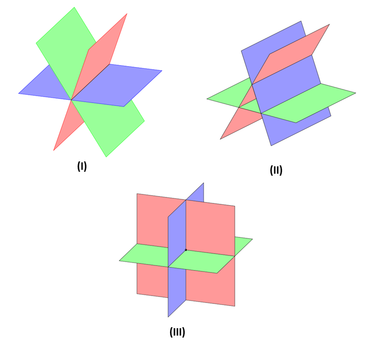
Figure 1: Three mutually non-parallel planes in $\mathbb{R}^{3}$ can intersect each other in three different ways. While in case (I) all three planes intersect in a common line, in case (II) each of the pairs intersect in different lines. On the other hand, in case (III) they intersect in a common unique point, which is of our interest.

To find the extreme points of the normalized state space, first note that the inequality $\operatorname{Tr}[e(\Phi)]\geq 0$ represents an $8$-dimensional half-space for any normalized state $\Phi$ and for any effect $e\in\mathcal{P}_{ef}[n]$. If we represent this expression as an equality, i.e., $\operatorname{Tr}[e(\Phi)]=0$, then it corresponds to a $7$-dimensional hyper-surface. Now for a different $e^{\prime}\in\mathcal{P}_{ef}[n]$ the equation $\operatorname{Tr}[e^{\prime}(\Phi)]=0$ corresponds to another $7$-dimensional hyper-surface which is either parallel to the hyper-surface corresponding to the effect $e$ or they intersect each other in a $6$-dimensional hyper-surface. Now for a third effect $e^{\prime\prime}$, if the $7$-dimensional hyper-surface $\operatorname{Tr}[e^{\prime\prime}(\Phi)]=0$ is not parallel to the hyper-surfaces corresponding to $e$ and $e^{\prime}$ then it may intersect them in the same $6$-dimensional hyper-surface (the intersection of $\operatorname{Tr}[e(\Phi)]=0$ and $\operatorname{Tr}[e^{\prime}(\Phi)]=0$ hyper-surfaces) or these three intersect each other in a $5$-dimensional hyper-surface (see Fig.1). By proceeding this way, at some stage, $8$ different hyper-surface corresponding to eight different effects from $\mathcal{P}_{ef}[n]$ will intersect at a single point, which corresponds to a normalized pure state. Mathematically this boils downs to checking the uniqueness of the solution for a system of linear equations. The eight different effects from the set $\mathcal{P}_{ef}[n]$ can be chosen in ${}^{n^{2}}C_{8}$ different ways. All of these choices will not lead to a unique solution, but whenever it does, we obtain an extremal bipartite state for the maximal composition of the polygonal systems, provided the positivity constraints are satisfied. See the Appendix for a more detailed discussion.

Once an extreme state $\Phi$ is identified, it is then straightforward to check whether it belongs to the set $\mathcal{P}_{st}[n]$ or not. If it does not belong to the set $\mathcal{P}_{st}[n]$, it corresponds to an extreme entangled state. Furthermore, the entangled states can be classified (see Definition 1) with the help of local reversible operations chosen from the set $\mathcal{T}_{AB}[n]$.

III.2 Bipartite pentagon system

Following the above procedure in MATLAB, for bipartite composition of pentagon systems we obtain $135$ different extreme states $\Phi_{k}$; $k\in\{1,2,\cdots,135\}$. Among these we have $25$ (say, number $1$ to $25$) factorized extreme states $\Phi_{5(i-1)+j}=\omega_{i}\otimes\omega_{j}^{\mathrm{T}}$, where $i,j\in\{1,\cdots,5\}$ and $\omega_{i}$’s are given in Eq.(1). The remaining $110$ states (number $26$ to $135$) are entangled. Furthermore, applying the local reversible transformation we find that these states divides into two classes – (i) the first class contains $10$ states (say, number $26$ to $35$), and (ii) the second one contains $100$ states (number $36$ to $135$). One representation state of the first class is the state $\Phi_{J}$ of Eq.(6) and hence we call this Janotta class. One of the representation state for the second class is given by

$$\Phi_{H}=\begin{pmatrix}-\cos(\pi/5)&\frac{-r_{5}^{6}\sin(\pi/5)}{8\left(1+r_{5}^{2}\right)}&0\\ \frac{-r_{5}^{6}\sin(\pi/5)}{8\left(1+r_{5}^{2}\right)}&\cos(\pi/5)&\frac{-r_{5}^{3}}{4\sin(\pi/5)}\\ 0&\frac{-r_{5}^{3}}{4\sin(\pi/5)}&1\\ \end{pmatrix}.$$ (11)

This class we call the Hardy class, so the sub-index ‘H’. The justification of this nomenclature will become obvious in the next section. The other states in Janotta class and Hardy class can be obtained from the representative states $\Phi_{J}$ and $\Phi_{H}$ respectively by applying local reversible transformations.

The two classes of states $\Phi_{J}$ and $\Phi_{H}$ have structural distinctions. For instance the state in Eq.(6) we have $a_{3}=a_{6}=a_{7}=a_{8}=0$. It can be shown that all the states in this class (obtained through local reversible transformations) have the same feature, which is not the case for the states in the class of $\Phi_{H}$.

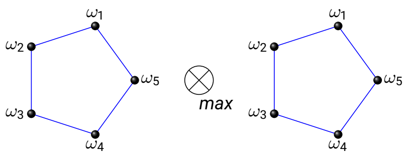
Figure 2: Maximal tensor product of two elementary pentagon systems allows $25$ product states. On the other hand, it allows two different classes (not equivalent under local reversible transformation) of entangled states: Janotta class states with $\Phi_{J}$ of Eq.(6) being a representative state and the Hardy class states with $\Phi_{H}$ of Eq.(11). While $\Phi_{J}$ can be thought of as a natural analog of the maximally entangled state of a two-qubit and does not exhibit Hardy’s nonlocality, the $\Phi_{H}$ state show Hardy and importantly with the success probability strictly greater than quantum success. However, the resulting correlation belongs to the set of almost quantum set $Q_{1}$.

III.3 Bipartite hexagon system

The task of characterizing all the entangled states becomes computationally costly with higher gons. This is because the choices of eight different effects rapidly increase with the number of sides in the component polygons. However, we obtain a complete characterization of the entanglement states for the bipartite hexagon. It turns out that there are six different entangled classes of states possible there. Representation states for each of these classes are given below:

$$\Phi_{I} =\begin{pmatrix}\cos\frac{\pi}{6}&\sin\frac{\pi}{6}&0\\ -\sin\frac{\pi}{6}&\cos\frac{\pi}{6}&0\\ 0&0&1\end{pmatrix},\leavevmode\nobreak\ \Phi_{II}=\begin{pmatrix}\frac{1}{15r_{6}^{2}}&\frac{7}{10}&\frac{2}{3r_{6}^{3}}\\ \frac{7}{10}&\frac{1}{5r_{6}^{2}}&\frac{3}{5r_{6}}\\ \frac{2}{3r_{6}^{3}}&\frac{3}{5r_{6}}&1\end{pmatrix},$$

$$\Phi_{III} =\begin{pmatrix}\frac{-1}{3r_{6}^{2}}&\frac{-1}{r_{6}^{4}}&\frac{2}{3r_{6}^{3}}\\ \frac{-1}{r_{6}^{4}}&0&\frac{1}{2r_{6}}\\ \frac{-2}{3r_{6}^{3}}&\frac{-1}{2r_{6}}&1\end{pmatrix},\leavevmode\nobreak\ \leavevmode\nobreak\ \leavevmode\nobreak\ \leavevmode\nobreak\ \leavevmode\nobreak\ \leavevmode\nobreak\ \leavevmode\nobreak\ \leavevmode\nobreak\ \Phi_{IV}=\begin{pmatrix}\frac{1}{7r_{6}^{2}}&\frac{9}{14}&\frac{10}{21r_{6}^{3}}\\ \frac{11}{14}&\frac{1}{7r_{6}^{2}}&\frac{5}{7r_{6}}\\ \frac{6}{7r_{6}^{3}}&\frac{3}{7r_{6}}&1\end{pmatrix},$$ (12)

$$\Phi_{V} =\begin{pmatrix}\frac{1}{7r_{6}^{2}}&\frac{11}{14}&\frac{6}{7r_{6}^{3}}\\ \frac{9}{14}&\frac{1}{7r_{6}^{2}}&\frac{3}{7r_{6}}\\ \frac{10}{21r_{6}^{3}}&\frac{5}{7r_{6}}&1\end{pmatrix},\leavevmode\nobreak\ \leavevmode\nobreak\ \leavevmode\nobreak\ \leavevmode\nobreak\ \leavevmode\nobreak\ \leavevmode\nobreak\ \Phi_{VI}=\begin{pmatrix}\frac{-1}{2r_{6}^{2}}&\frac{-1}{r_{6}^{4}}&\frac{1}{3r_{6}^{3}}\\ \frac{-1}{r_{6}^{4}}&\frac{1}{2r_{6}^{2}}&\frac{-1}{2r_{6}}\\ \frac{1}{3r_{6}^{3}}&\frac{-1}{2r_{6}}&1\end{pmatrix}.$$

The state $\Phi_{I}$ is the maximally entangled state $\Phi_{J}$ of Eq.(7) as identified by Janotta et al. Important to note that the state $\Phi_{II},\leavevmode\nobreak\ \Phi_{III},\leavevmode\nobreak\$ and $\Phi_{VI}$ are symmetric states, while the other three are not. Recall that, a joint state $\Phi^{AB}$ is called symmetric if $(e\otimes f)(\Phi^{AB})=(f\otimes e)(\Phi^{AB}),\leavevmode\nobreak\ \forall\leavevmode\nobreak\ e,f\in V^{\star}_{+}$, and in matrix representation $\Phi^{AB}$ is symmetric if and only if the corresponding matrix is symmetric [14].

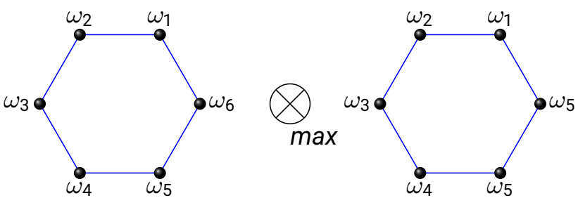
Figure 3: Maximal tensor product of two elementary hexagon systems allows $36$ product state. On the other hand, it allows six different classes of entangled states. Representative states for each of the classes are given in Eq.(III.3). The state $\Phi_{I}$ although can be thought of as an analog of the maximally entangled state, but unlike the two-qubit maximally entangled state, it exhibits Hardy’s nonlocality behaviour.

IV Nonlocal properties of the entangled states

Nonlocal properties of the correlations obtained from the maximally entangled states $\Phi_{J}$ have been studied in Ref. [14]. In particular, the maximal CHSH inequality violation has been explored for even and odd gons. Importantly, the correlations of even $n$ systems can always reach or exceed Tsirelson’s bound, while the correlations of odd $n$ systems are always below Tsirelson’s bound. For the odd $n$ systems the maximally entangled state belongs to the class inner product states and all correlations obtainable from measurements on inner product states satisfy Tsirelson’s bound. Here we analyze the nonlocal properties of different classes of entangled states from the perspective of Hardy’s nonlocality argument.

As already mentioned we need two dichotomic measurements both on Alice’s and Bob’s part to construct the Hardy’s non-locality argument. Furthermore, Alice (also Bob) must choose incompatible measurements on her (his) subsystem [44, 45]. Let Alice’s first measurement is $\mathcal{M}_{1}^{A}=\left\{e_{i}^{A},\bar{e}_{i}^{A}\right\}\equiv\left\{E^{A+}_{1},E^{A-}_{1}\right\}$. We use the notation $\mathcal{M}_{1}^{A}=\left\{E^{A+}_{1},E^{A-}_{1}\right\}$ to give the freedom that positive outcome can be assigned to $e^{A}_{i}$ or $\bar{e}^{A}_{i}$. The other measurement of Alice be $\mathcal{M}_{2}^{A}=\left\{e_{j}^{A},\bar{e}_{j}^{A}\right\}\equiv\left\{E^{A+}_{2},E^{A-}_{2}\right\}$, with $j\neq i$. Similarly, for Bob let us consider two measurements $\mathcal{M}_{1}^{B}=\left\{e_{k}^{B},\bar{e}_{k}^{B}\right\}\equiv\left\{E^{B+}_{1},E^{B-}_{1}\right\}$ and $\mathcal{M}_{2}^{B}=\left\{e_{l}^{B},\bar{e}_{l}^{B}\right\}\equiv\left\{E^{B+}_{2},E^{B-}_{2}\right\}$, with $l\neq k$. With this measurement choices, up-to local relabelings, the Hardy’s nonlocality argument can be written as

$$P(E^{A+}_{1},E^{B+}_{1}|\mathcal{M}_{1}^{A}\mathcal{N}_{1}^{B})>0,$$ (13a)

$$P(E^{A+}_{1},E^{B+}_{2}|\mathcal{M}_{1}^{A}\mathcal{N}_{2}^{B})=0,$$ (13b)

$$P(E^{A+}_{2},E^{B+}_{1}|\mathcal{M}_{2}^{A}\mathcal{N}_{1}^{B})=0,$$ (13c)

$$P(E^{A-}_{2},E^{B-}_{2}|\mathcal{M}_{2}^{A}\mathcal{N}_{2}^{B})=0.$$ (13d)

IV.1 Hardy’s nonlocality for maximally entangled states

In this subsection, we will analyze Hardy’s nonlocality behaviour of the correlations obtained from the maximally entangled states of bipartite polygon theories. We prove two generic results. In the following, we first prove a no-go result.

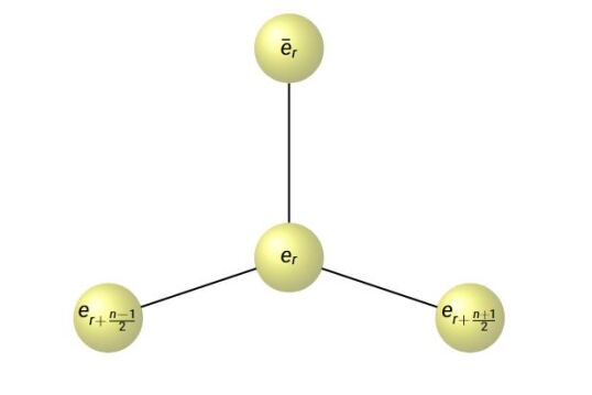
Figure 4: (Color online) Orthogonality graph of extreme effects for odd-gon theories. Each node denotes an extreme effect. Two effects $e$ and $f$ are connected with each other by an edge if and only if they are orthogonal to each other in the sense that $e\cdot f=0$; here, the inner product is standard $\mathbb{R}^{3}$ inner product. Operationally, for a pair of such effects there always exist at least one pair of states $\omega_{e}$ and $\omega_{f}$, such that $e\cdot\omega_{e}=1=f\cdot\omega_{f}$ and $e\cdot\omega_{f}=0=f\cdot\omega_{e}$. While calculating the sub-indices of the effects modulo $n$ operation is assumed throughout.

Theorem 1.

The maximally entangled states $\Phi_{J}$ of the bipartite regular polygons with odd $n$ do not exhibit Hardy’s nonlocality argument.

Proof.

The outcome probability for any pair of effect $E$ on Alice’s side and $F$ on Bob’s side for the maximally entangled state $\Phi_{J}$ of Eq.(6) read as

$$P_{\Phi_{J}}(E,F) =\operatorname{Tr}\left[\left(E\otimes F^{\mathrm{T}}\right)\Phi_{J}^{\mathrm{T}}\right]$$

$$=\operatorname{Tr}\left[E\otimes F^{\mathrm{T}}\right]=E\cdot F,$$ (14)

where $E\cdot F$ be the usual inner product in $\mathbb{R}^{3}$. With this, the Hardy conditions of Eq.(13) become

$$P(E^{A+}_{1},E^{B+}_{1}|\mathcal{M}_{1}^{A}\mathcal{N}_{1}^{B})=E^{A+}_{1}\cdot E^{B+}_{1}>0,$$ (15a)

$$P(E^{A+}_{1},E^{B+}_{2}|\mathcal{M}_{1}^{A}\mathcal{N}_{2}^{B})=E^{A+}_{1}\cdot E^{B+}_{2}=0,$$ (15b)

$$P(E^{A+}_{2},E^{B+}_{1}|\mathcal{M}_{2}^{A}\mathcal{N}_{1}^{B})=E^{A+}_{2}\cdot E^{B+}_{1}=0,$$ (15c)

$$P(E^{A-}_{2},E^{B-}_{2}|\mathcal{M}_{2}^{A}\mathcal{N}_{2}^{B})=E^{A-}_{2}\cdot E^{B-}_{2}=0.$$ (15d)

To see whether the aforesaid conditions can be satisfied in any odd-gon, it is handy to have a look at the orthogonality graph for the extreme effects of the odd-gon theory. Two effects $e$ and $f$ will be called orthogonal to each other if and only if $e\cdot f=0$. In any odd gon theory, it turns out that a ray extremal effect $e_{r}$ is orthogonal to the only two other ray extremely effects $e_{s^{\pm}}$, with $s^{\pm}:=\left(r+\frac{n\pm 1}{2}\right)\leavevmode\nobreak\ \mbox{mod}\leavevmode\nobreak\ n$; and to the (non-ray) extremal effect $\bar{e}_{r}$. The orthogonality graph is shown in Fig. 3. The proof of the theorem follows by analyzing the following two cases.

Case-I: Let us assume that the effect $E^{B+}_{2}$ in Eq.(15b) corresponds to some ray extremal effect (say) $e_{r}$. This implies $E^{B-}_{2}=\bar{e}_{r}$, since $\{E^{B+}_{2},E^{B-}_{2}\}$ correspond to a measurement. Eq.(15d) further implies that $E^{A-}_{2}$ must be orthogonal to $E^{B-}_{2}$. Since the only extreme effect orthogonal to $\bar{e}_{r}$ is $e_{r}$ (see Fig. 3), therefore we must have $E^{A-}_{2}=e_{r}$, which further implies $E^{A+}_{2}=\bar{e}_{r}$. Again Eq.(15c) implies $E^{B+}_{1}=e_{r}$ and hence $E^{A+}_{1}\cdot E^{B+}_{1}=E^{A+}_{1}\cdot E^{B+}_{2}=0$, implying zero Hardy success.

Case-II: Here we start by assuming that the effect $E^{B+}_{2}$ in Eq.(15b) corresponds to some non ray extremal effect (say) $\bar{e}_{r}$. This implies $E^{B-}_{2}=e_{r}$, since $\{E^{B+}_{2},E^{B-}_{2}\}$ correspond to a measurement. This also implies $E^{A+}_{1}=e_{r}$ from Eq.(15b). Now from Eq.(15d) we know that $E^{A-}_{2}$ is orthogonal to $E^{B-}_{2}$. Which implies either $E^{A-}_{2}=e_{s^{\pm}}$ $\left(\mbox{with}\leavevmode\nobreak\ s^{\pm}:=\left(r+\frac{n\pm 1}{2}\right)\leavevmode\nobreak\ \mbox{mod}\leavevmode\nobreak\ n\right)$ or $E^{A-}_{2}=\bar{e}_{r}$. If $E^{A-}_{2}=e_{s^{\pm}}$ we have $E^{A+}_{2}=\bar{e}_{s^{\pm}}$ since $\{E^{A+}_{2},E^{A-}_{2}\}$ forms a measurement. Which from Eq.(15c) further implies $E^{B+}_{1}=e_{s^{\pm}}$, yielding $E^{A+}_{1}\cdot E^{B+}_{1}=\bar{e}_{r}\cdot e_{s^{\pm}}=0$. Similarly if $E^{A-}_{2}=\bar{e}_{r}$ we would get $E^{A+}_{2}=e_{r}$ and $E^{A+}_{1}\cdot E^{B+}_{1}=E^{A+}_{2}\cdot E^{B+}_{1}=0$. This proves that even for Case-II we have zero Hardy success, and hence completes the proof. ∎

While maximally entangled states of bipartite odd gons do not exhibit Hardy’s nonlocality, maximally entangled states of bipartite square bit do exhibit such nonlocality. The PR box correlation resulting from the maximally entangled state of bipartite square bit exhibits Hardy’s nonlocality argument with success probability $1/2$, which is, in fact, the maximum Hardy’s success among any no-signaling correlations. In the following, we prove a generic result that the maximally entangled state of any bipartite even gon depicts Hardy’s type of nonlocality, albeit with decreasing success probability.

At this point, it is worth mentioning that the maximally entangled state of the quantum two-qubit system fails to exhibit Hardy’s nonlocality behaviour [11]. In this sense, odd gons are more close to quantum than the even gons as the maximally entangled states of the former do not depict Hardy nonlocality while the latter do.

Theorem 2.

The maximally entangled state $\Phi_{J}$ of bipartite even-gons (with $n\geq 4$) exhibits Hardy’s non-locality argument with the success probability given by $\sin^{2}(\pi/n)$.

Proof.

For even-gons all the extreme effects are ray extremal. The outcome probability $P_{\Phi_{J}}\left(e_{i}^{A},e_{j}^{B}\right)$ of Alice’s effect $e_{i}^{A}$ and Bob’s effect $e_{j}^{B}$ on the maximally entangled state $\Phi_{j}$ of Eq.(7) reads as

$$P_{\Phi_{J}}\left(e_{i}^{A},e_{j}^{B}\right) =\operatorname{Tr}\left[\left(e_{i}\otimes e_{j}^{\mathrm{T}}\right)\Phi_{J}\right]$$

$$=\frac{1}{4}\left[\sec\left(\frac{\pi}{n}\right)\cos\left(\frac{2(i-j)\pi}{n}-\frac{\pi}{n}\right)\right]+\frac{1}{4}.$$

Now $P_{\Phi_{J}}\left(e_{i}^{A},e_{j}^{B}\right)=0$ if and only if

$$\cos\left(\frac{2(i-j)\pi}{n}-\frac{\pi}{n}\right) =-\cos\left(\frac{\pi}{n}\right)$$

$$i.e.,\leavevmode\nobreak\ i-j =\frac{1}{2}+\frac{n\pm 1}{2},$$ (16)

where in the last expression modulo $n$ addition is implied. Let us consider $E^{A+}_{1}$ in Eq.(13) be some ray extremal effect $e_{r}$ for some $r\in\{1,2,\cdots,n\}$. Eq.(16) implies that to satisfy the condition of Eq.(13b), we must have $E^{B+}_{2}=e_{s(\alpha)}$, where $s(\alpha)=r-\frac{(n+1)}{2}+(-1)^{\alpha}\frac{1}{2}$, with Greek indices taking values from $\{0,1\}$. Since $E^{B+}_{2}$ and $E^{B-}_{2}$ forms a measurement, therefore we have $E^{B+}_{2}=e_{t(\alpha)}$, where $t(\alpha)=r-\frac{1}{2}+(-1)^{\alpha}\frac{1}{2}$. Again, Eqs.(16) and (13d) imply $E^{A-}_{2}=e_{v(\alpha,\beta)}$, where $v(\alpha,\beta)=r+[(-1)^{\alpha}+(-1)^{\beta}]\frac{1}{2}+\frac{n}{2}$, and $E^{A+}_{2}=e_{w(\alpha,\beta)}$, with $w(\alpha,\beta)=r+[(-1)^{\alpha}+(-1)^{\beta}]\frac{1}{2}$. Finally, Eqs.(16) and (13c) yield $E^{B+}_{1}:=e_{z(\alpha,\beta,\gamma)}=r+[(-1)^{\alpha}+(-1)^{\beta}+(-1)^{\gamma}]\frac{1}{2}-\frac{1}{2}-\frac{n}{2}$. In other words, given the choice $E^{A+}_{1}=e_{r}$ the effect $E^{B+}_{1}$ has only the following four choices

$$E^{B+}_{1} =e_{z(\alpha)};\leavevmode\nobreak\ z(\alpha):=r-\frac{(n+1)}{2}+(-1)^{\alpha}\frac{1}{2},$$ (17a)

$$E^{B+}_{1} =e_{z(\alpha)};\leavevmode\nobreak\ z(\alpha):=r-\frac{(n+1)}{2}+(-1)^{\alpha}\frac{3}{2}.$$ (17b)

For the case of Eq.(17a), we have

$$P_{\Phi_{J}}\left(E^{A+}_{1},E^{B+}_{1}\right)$$

$$=\frac{1}{4}\left[\sec\left(\frac{\pi}{n}\right)\cos\left(\frac{2(r-z(\alpha))\pi}{n}-\frac{\pi}{n}\right)\right]+\frac{1}{4}$$

$$=\frac{1}{4}\left[\sec\left(\frac{\pi}{n}\right)\cos\left(\frac{2(\frac{n}{2}+\frac{1}{2}\pm\frac{1}{2})\pi}{n}-\frac{\pi}{n}\right)\right]+\frac{1}{4}$$

$$=\frac{1}{4}\left[\sec\left(\frac{\pi}{n}\right)\cos\left(\pi\pm\frac{\pi}{n}\right)\right]+\frac{1}{4}$$

$$=\frac{1}{4}\left[-\sec\left(\frac{\pi}{n}\right)\cos\left(\frac{\pi}{n}\right)\right]+\frac{1}{4}=0.$$

Therefore, these particular choices of $E^{B+}_{1}$ do not exhibit Hardy nonlocality. However, for the choices of Eq.(17b) we obtain

$$P_{\Phi_{J}}\left(E^{A+}_{1},E^{B+}_{1}\right)$$

$$=\frac{1}{4}\left[\sec\left(\frac{\pi}{n}\right)\cos\left(\frac{2(r-z(\alpha))\pi}{n}-\frac{\pi}{n}\right)\right]+\frac{1}{4}$$

$$=\frac{1}{4}\left[\sec\left(\frac{\pi}{n}\right)\cos\left(\frac{2(\frac{n}{2}+\frac{1}{2}\pm\frac{3}{2})\pi}{n}-\frac{\pi}{n}\right)\right]+\frac{1}{4}$$

$$=\frac{1}{4}\left[\sec\left(\frac{\pi}{n}\right)\cos\left(\pi\pm\frac{3\pi}{n}\right)\right]+\frac{1}{4}$$

$$=\frac{1}{4}\left[-\sec\left(\frac{\pi}{n}\right)\cos\left(\frac{3\pi}{n}\right)\right]+\frac{1}{4}=\sin^{2}\left(\frac{\pi}{n}\right).$$

This completes the proof of the theorem. The variation of the Hardy’s success probability for different even gons is shown in Fig. 5. ∎

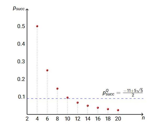
Figure 5: (Color online) Red dots denote the maximum success probability of Hardy’s nonlocality argument for maximally entangled states of bipartite even gons. The Blue dashed line denotes the optimal quantum success probability of Hardy’s nonlocality argument.

IV.2 Hardy’s nonlocality for non-maximally entangled states

For bipartite pentagon case we only have two inequivalent classes of pure entangled states, the state $\Phi_{J}$ of Eq.(6) and the state $\Phi_{H}$ of Eq.(11). As already established in Theorem 1, the state $\Phi_{J}$ cannot result in any correlation exhibiting Hardy’s nonlocality. So the natural question arises whether the state $\Phi_{H}$ can lead to such a correlation. Interestingly we find that that state $\Phi_{H}$ indeed exhibits Hardy’s nonlocality. If we consider two incompatible measurements $\mathcal{M}_{1}\equiv\{e_{1},\bar{e}_{1}\}$ and $\mathcal{M}_{2}\equiv\{e_{5},\bar{e}_{5}\}$ on Alice’s part and two incompatible measurements $\mathcal{N}_{1}\equiv\{e_{1},\bar{e}_{1}\}$ and $\mathcal{N}_{2}\equiv\{\bar{e}_{2},e_{2}\}$ on Bob’s part, the resulting correlation depicts Hardy’s nonlocality. Denoting the outcome corresponding to the first effect as $+1$ and the outcome corresponding to the second one as $-1$, the correlation obtained from theses choices of measurements reads as

$$\mathbf{P}\leavevmode\nobreak\ \equiv\leavevmode\nobreak\ \begin{array}[]{c||c|c|c|c|}&(+,+)&(+,-)&(-,+)&(-,-)\\ \hline\cr\hline\cr\mathcal{M}_{1}\mathcal{N}_{1}&{\color[rgb]{0,0,1}1-\frac{4\sqrt{5}}{10}}&\frac{7\sqrt{5}}{10}-\frac{3}{2}&\frac{7\sqrt{5}}{10}-\frac{3}{2}&3-\sqrt{5}\\ \hline\cr\mathcal{M}_{1}\mathcal{N}_{2}&{\color[rgb]{0,0,1}0}&\frac{3\sqrt{5}}{10}-\frac{1}{2}&\frac{\sqrt{5}}{10}+\frac{1}{2}&1-\frac{4\sqrt{5}}{10}\\ \hline\cr\mathcal{M}_{2}\mathcal{N}_{1}&{\color[rgb]{0,0,1}0}&\frac{2\sqrt{5}}{10}&\frac{3\sqrt{5}}{10}-\frac{1}{2}&\frac{3}{2}-\frac{5\sqrt{5}}{10}\\ \hline\cr\mathcal{M}_{2}\mathcal{N}_{2}&\frac{3\sqrt{5}}{10}-\frac{1}{2}&\frac{1}{2}-\frac{\sqrt{5}}{10}&1-\frac{2\sqrt{5}}{10}&{\color[rgb]{0,0,1}0}\\ \hline\cr\end{array}\leavevmode\nobreak\ .$$ (23)

Important to note that the success probability of Hardy’s argument in this case is $P\left(+,+|\mathcal{M}_{1}\mathcal{N}_{1}\right)=1-\frac{4\sqrt{5}}{10}\approx 0.1056$, which is strictly larger than the corresponding optimal quantum value $\frac{5\sqrt{5}-11}{2}\approx 0.0902$. Therefore, this particular correlation is beyond quantum in nature, although its CHSH value is strictly less than the Cirel’son’s value. The success probability $0.1056$ turns out to be optimal in pentagon theory. However, the same state exhibit Hardy’s nonlocality with the success probability $\frac{7\sqrt{5}}{10}-\frac{3}{2}\approx 0.0652$ for same choices of measurements on Alice’s side but a different choices of measurements $\mathcal{N}^{\prime}_{1}\equiv\{\bar{e}_{3},e_{3}\}$ and $\mathcal{N}^{\prime}_{2}\equiv\{\bar{e}_{2},e_{2}\}$ on Bob’s side. The resulting correlation in this case reads as

$$\mathbf{P}^{\prime}\leavevmode\nobreak\ \equiv\leavevmode\nobreak\ \begin{array}[]{c||c|c|c|c|}&(+,+)&(+,-)&(-,+)&(-,-)\\ \hline\cr\hline\cr\mathcal{M}_{1}\mathcal{N}^{\prime}_{1}&{\color[rgb]{0,0,1}\frac{7\sqrt{5}}{10}-\frac{3}{2}}&{1-\frac{4\sqrt{5}}{10}}&{3-\frac{12\sqrt{5}}{10}}&\frac{9\sqrt{5}}{10}-\frac{3}{2}\\ \hline\cr\mathcal{M}_{1}\mathcal{N}^{\prime}_{2}&{\color[rgb]{0,0,1}0}&\frac{3\sqrt{5}}{10}-\frac{1}{2}&\frac{\sqrt{5}}{10}+\frac{1}{2}&1-\frac{4\sqrt{5}}{10}\\ \hline\cr\mathcal{M}_{2}\mathcal{N}^{\prime}_{1}&{\color[rgb]{0,0,1}0}&\frac{2\sqrt{5}}{10}&\frac{3}{2}-\frac{5\sqrt{5}}{10}&\frac{3\sqrt{5}}{10}-\frac{1}{2}\\ \hline\cr\mathcal{M}_{2}\mathcal{N}^{\prime}_{2}&\frac{3\sqrt{5}}{10}-\frac{1}{2}&\frac{1}{2}-\frac{\sqrt{5}}{10}&1-\frac{2\sqrt{5}}{10}&{\color[rgb]{0,0,1}0}\\ \hline\cr\end{array}\leavevmode\nobreak\ .$$

For the hexagon case, we find that all the six different classes of states depicts Hardy’s nonlocality. The choices of measurements and the corresponding Hardy’s success probabilities are listed in Table 1.

State	Alice’s	Bob’s	Hardy’s
	Measurements	Measurements	Success
$\Phi_{I}$	$\mathcal{M}_{1}=\{e_{1},e_{4}\}$	$\mathcal{N}_{1}=\{e_{6},e_{3}\}$	1/4
	$\mathcal{M}_{2}=\{e_{2},e_{5}\}$	$\mathcal{N}_{2}=\{e_{5},e_{2}\}$
$\Phi_{II}$	$\mathcal{M}_{1}=\{e_{4},e_{1}\}$	$\mathcal{N}_{1}=\{e_{4},e_{1}\}$	1/20
	$\mathcal{M}_{2}=\{e_{2},e_{5}\}$	$\mathcal{N}_{2}=\{e_{2},e_{5}\}$
$\Phi_{III}$	$\mathcal{M}_{1}=\{e_{3},e_{6}\}$	$\mathcal{N}_{1}=\{e_{1},e_{4}\}$	1/16
	$\mathcal{M}_{2}=\{e_{2},e_{5}\}$	$\mathcal{N}_{2}=\{e_{6},e_{3}\}$
	$\mathcal{M}_{1}=\{e_{4},e_{1}\}$	$\mathcal{N}_{1}=\{e_{1},e_{4}\}$	1/8
	$\mathcal{M}_{2}=\{e_{2},e_{5}\}$	$\mathcal{N}_{2}=\{e_{5},e_{2}\}$
$\Phi_{IV}$	$\mathcal{M}_{1}=\{e_{3},e_{6}\}$	$\mathcal{N}_{1}=\{e_{4},e_{1}\}$	1/28
	$\mathcal{M}_{2}=\{e_{2},e_{5}\}$	$\mathcal{N}_{2}=\{e_{3},e_{6}\}$
	$\mathcal{M}_{1}=\{e_{4},e_{1}\}$	$\mathcal{N}_{1}=\{e_{4},e_{1}\}$	1/14
	$\mathcal{M}_{2}=\{e_{2},e_{5}\}$	$\mathcal{N}_{2}=\{e_{2},e_{5}\}$
$\Phi_{V}$	$\mathcal{M}_{1}=\{e_{4},e_{1}\}$	$\mathcal{N}_{1}=\{e_{3},e_{6}\}$	1/28
	$\mathcal{M}_{2}=\{e_{3},e_{5}\}$	$\mathcal{N}_{2}=\{e_{2},e_{5}\}$
	$\mathcal{M}_{1}=\{e_{4},e_{1}\}$	$\mathcal{N}_{1}=\{e_{4},e_{1}\}$	1/14
	$\mathcal{M}_{2}=\{e_{2},e_{5}\}$	$\mathcal{N}_{2}=\{e_{2},e_{5}\}$
$\Phi_{VI}$	$\mathcal{M}_{1}=\{e_{2},e_{5}\}$	$\mathcal{N}_{1}=\{e_{2},e_{5}\}$	1/8
	$\mathcal{M}_{2}=\{e_{1},e_{4}\}$	$\mathcal{N}_{2}=\{e_{1},e_{4}\}$

Table 1: Measurement choices for Alice and Bob and the corresponding Hardy’s success probabilities for the six different classes of entangled states in bipartite hexagon theory.

The problem of singling out Quantum correlations from the other possible no-signalling correlations is an active area of research in the quantum foundation. It has been shown that Quantum theory is not so unique as expected when the input-output correlations among different systems are considered. There exist no-signalling correlations that are beyond quantum in nature but satisfy all the device-independent principles proposed so far to single out Quantum correlations, and the set of such correlations is known as ‘almost quantum correlations’ ($Q_{1}$). [46]. It is also known that correlations in $Q_{1}$ can not be distilled outside the set $Q_{1}$ under local operation and shared randomness [Navascues10], and these correlations respect Tsirelson’s bound of $2\sqrt{2}$. Maximally entangled states of the even gons yield correlations exceeding the Tsirelson’s bound and hence lie outside $Q_{1}$. On the other hand, the maximally entangled states of odd gons being inner product states yield correlation lying within $Q_{1}$ [14]. Using the efficient method of semi-definite programming (SDP), [46] we find that the correlation in Eq.(IV.2) belongs to $Q_{1}$ although, from the success probability of Hardy’s nonlocality, we know it is a beyond quantum correlation.

IV.3 Mixed entangled state and Hardy’s nonlocality

Here we observe an interesting aspect of Hardy’s nonlocality, which makes a sharp distinction between the two-qubit system and the bipartite polygon models. Recall that mixed states of two-qubit systems do not exhibit Hardy-type nonlocality [12]. However, in the polygonal counterparts, we will show that this is not the case. Note that, while a local correlation can not exhibit Hardy-type nonlocality, there exist such local strategies for which all four probabilities are exactly zero. On the other hand, a two-qubit separable state can exhibit such a local correlation only if the spatially separated parties perform compatible measurements on their respective constituents. Measurement incompatibility being necessary for any nonlocal argument [12, 47, 48], hence forbids the mixed entangled two-qubit states to exhibit Hardy-type nonlocality.

Theorem 3.

For every even ($n$)-gon theory and $\forall\epsilon\in(0,1]$, there exists a class of mixed entangled states $W_{\epsilon}=\epsilon\Phi_{J}+(1-\epsilon)\omega_{i}\otimes\omega_{j}$ exhibiting Hardy nonlocality.

Proof.

From Theorem 2 it follows that to obtain a Hardy nonlocal behaviour from the state $\Phi_{J}$ it requires $E_{1}^{A+}=e_{r}$ then $E_{2}^{A+}=e_{r\pm 1}$. In an even-gon theory every two consecutive effects $e_{i}$ and $e_{i\oplus_{n}1}$ click with certainty on the state $\omega_{i}$ and they never click on state $\omega_{i\oplus_{n}n}$ (here modulo operation is same as defined in footnote of page 7). Therefore, $\forall r\in\{1,2,\cdots,n\}$ there is a state $\omega_{r}\in\Omega^{A}$ in Alice’s side, such that $\operatorname{Tr}((E_{1}^{A+})^{T}\omega_{r})=\operatorname{Tr}((E_{2}^{A+})^{T}\omega_{r})=0$. Similarly, there is a state $\omega_{s}\in\Omega^{B}$, such that $\operatorname{Tr}((E_{2}^{B-})^{T}\omega_{s})=0$. Evidently, the state $\omega_{r}\otimes\omega_{s}$ satisfies all the conditions Eq. (15b)-(15d) and equals to zero for Eq. (15a). So, for the state $W_{\epsilon}=\epsilon\Phi_{J}+(1-\epsilon)\omega_{r}\otimes\omega_{s}$, with $\epsilon\in(0,1]$, all the conditions (15b) - (15d) are satisfied, with $\operatorname{Tr}[(E_{1}^{A+}\otimes E_{1}^{B+})^{\mathrm{T}}W_{\epsilon}]=\epsilon\times\sin^{2}(\frac{\pi}{n})$. Clearly, for $\epsilon\neq 1$, the state $W_{\epsilon}$ is a mixed state and hence establish the claim of the theorem. ∎

In a similar spirit, it is possible to show that the mixed state of odd-gon theories can also exhibit Hardy’s nonlocality. In the following, we give a proof for the bipartite pentagon theory.

Theorem 4.

For every values of $\epsilon\in(0,1]$, the mixed entangled state $W_{\epsilon}=\epsilon\Phi_{H}+(1-\epsilon)\omega_{i}\otimes\omega_{j}$ exhibits Hardy-type nonlocality for suitable choice of measurement, whenever $\omega_{i}\otimes\omega_{j}\in\{\omega_{3}\otimes\omega_{4},\omega_{3}\otimes\omega_{5},\omega_{4}\otimes\omega_{3},\omega_{4}\otimes\omega_{4},\omega_{5}\otimes\omega_{3}\}$.

Proof.

If we consider two incompatible measurements $\mathcal{M}_{1}\equiv\{e_{1},\bar{e}_{1}\}$ and $\mathcal{M}_{2}\equiv\{\bar{e}_{2},e_{2}\}$ on Alice’s part and two incompatible measurements $\mathcal{N}_{1}\equiv\{e_{1},\bar{e}_{1}\}$ and $\mathcal{N}_{2}\equiv\{\bar{e}_{2},e_{2}\}$ on Bob’s part, then the resulting correlation obtained from the state $W_{\epsilon}$ depicts Hardy’s nonlocality, whenever $\omega_{i}\otimes\omega_{j}\in\{\omega_{3}\otimes\omega_{4},\omega_{4}\otimes\omega_{3},\omega_{4}\otimes\omega_{4}\}$. For $\omega_{i}\otimes\omega_{j}=\omega_{3}\otimes\omega_{5}$, we require the measurements $\mathcal{M}_{1}\equiv\{e_{1},\bar{e}_{1}\}$, $\mathcal{M}_{2}\equiv\{e_{5},\bar{e}_{5}\}$ on Alice’s part and $\mathcal{N}_{1}\equiv\{e_{1},\bar{e}_{1}\}$, $\mathcal{N}_{2}\equiv\{\bar{e}_{2},e_{2}\}$ on Bob’s part; and for $\omega_{i}\otimes\omega_{j}=\omega_{5}\otimes\omega_{3}$, $\mathcal{M}_{1}\equiv\{e_{1},\bar{e}_{1}\}$, $\mathcal{M}_{2}\equiv\{\bar{e}_{2},e_{2}\}$ on Alice’s side and $\mathcal{N}_{1}\equiv\{e_{1},\bar{e}_{1}\}$, $\mathcal{N}_{2}\equiv\{\bar{e}_{5},e_{5}\}$ on Bob’s side suffice the purpose. The success probability turns out to be $P^{succ}=\epsilon\times(1-\frac{4\sqrt{5}}{10})\approx 0.1056\epsilon$. ∎

While from the perspective of Bell-nonlocality, the polygonal state spaces exhibit no characteristic distinction (except the quantitative bounds) from their continuous counterpart QT, Theorem 3 and 4 exhibit such a distinction for Hardy-type nonlocal arguments. However, the signature of such a difference vanishes considering the bipartite compositions of higher quantum systems. In particular, for higher dimensional QT, there are incompatible local measurements with the proper choice of separable bipartite state, which can generate any of the extreme local correlations, and hence there are mixed entangled states depicting Hardy-type nonlocal arguments. This, in turn, direct towards the state space topology of the qubit system and the continuity therein to demonstrate it as unique among the possible two-dimensional state space structures.

V Inequivalence of entanglement and nonlocality in polygon models

While all bipartite quantum pure states exhibit nonlocality [49], the pure states are too idealistic when experimental situations are considered. So naturally the question arises whether mixed states exhibits such nonlocal behaviour. A particular family that are of interest to us is the Werner class of states

$$\mathcal{W}_{p}=p\ket{\psi^{-}}_{AB}\bra{\psi^{-}}+(1-p)\frac{\mathcal{I}}{2}\otimes\frac{\mathcal{I}}{2},$$ (24)

where $\ket{\psi^{-}}:=(\ket{01}-\ket{10})/\sqrt{2}\in\mathbb{C}^{2}\otimes\mathbb{C}^{2}$ and $p\in[-1/3,1]$. In particular, for $p\in[0,1]$ the state can be thought as statistical mixture of the singlet state and white noise. Straightforward calculation yields the state $\mathcal{W}_{p}$ is entangled for $p>\frac{1}{3}$ and violates CHSH inequality for $p>\frac{1}{\sqrt{2}}$. In a seminal result Werner established that for $<p\leq\frac{1}{2}$ the statistics obtained from the state $\mathcal{W}_{p}$ through local projective measurements can be explained by local hidden variable model [50]. Later Barrett has extended this model for arbitrary local measurement for the parameter range $p\leq\frac{5}{12}$ [51] (see also [52]). This result is quite important as it establishes that entanglement and nonlocality as two inequivalent notion. A similar question one can ask in polygon theories. Our next result partially address this question.

Theorem 5.

For all the theories where $n>4$, there exists a class of mixed entangled states that does not violate CHSH inequality.

Proof.

Consider the class of states, $\mathcal{W}^{O}_{p}:=p\Phi_{J}+(1-p)u\otimes u$, where $p\in[0,1]$ and $\Phi_{J}$ is the state given in Eq. (6). Clearly, $\mathcal{W}^{O}_{p}$ is a mixed state whenever $p\in[0,1)$.

For the odd-gons, the expectation value of any measurement $\langle\mathcal{M}_{i}\mathcal{N}_{j}\rangle$ on the maximally mixed state $u\otimes u$ reads as $\left(\frac{r_{n}^{2}-1}{r_{n}^{2}+1}\right)^{2}$. For the state $\mathcal{W}^{O}_{p}$ the maximum value of Bell-CHSH expression becomes $\mathbb{B}_{\max}(\mathcal{W}^{O}_{p})=p\mathbb{B}^{(n)}_{\max}+2(1-p)\left(\frac{r_{n}^{2}-1}{r_{n}^{2}+1}\right)^{2}$, where $\mathbb{B}^{(n)}_{\max}$ is the maximum Bell-CHSH value obtained from the $n$-gonal maximum entangled state $\Phi_{J}$. Denoting the range of the parameter $p_{NL}$ of the state $\mathcal{W}^{O}_{p}$ showing Bell-CHSH nonlocality we have

$$p_{NL}>8r_{n}^{2}\left[\mathbb{B}^{(n)}_{\max}\left(r_{n}^{2}+1\right)^{2}+\left(r_{n}^{2}-1\right)^{2}\right]^{-1}.$$ (25)

We now proceed to find the range of the parameter $p$ of the state $\mathcal{W}_{p}^{O}$ for which the state is entangled. Note that, unlike quantum theory, in this model, we do not have any criterion like negative partial transposition (NPT) [53, 54] that can detect the entanglement of a state. However, if we can find an effect that is entangled and yields a negative probability on some state, then by definition, the state must be entangled. This is because any product state on an entangled effect always gives a non-negative probability. For the odd-gon theory it has been shown that the effects $E_{ab}$ and $\bar{E}_{ab}:=u\otimes u-E_{ab}$ are entangled [19], where

$$E_{ab}=\frac{1}{1+r_{n}^{2}}\begin{pmatrix}1&0&0\\ 0&1&0\\ 0&0&1\end{pmatrix}.$$

A straightforward calculation yields $\operatorname{Tr}[\bar{E}_{ab}^{T}\mathcal{W}_{p}^{O}]=p\left(\frac{r_{n}^{2}-2}{1+r_{n}^{2}}\right)+(1-p)\frac{r_{n}^{2}}{1+r_{n}^{2}}$. Denoting the range of parameter of the state $\mathcal{W}_{p}^{O}$ as $p_{E}$ for which the state must be entangled we have

$$\operatorname{Tr}[\bar{E}_{ab}^{T}\mathcal{W}_{p_{E}}^{O}]<0\implies p_{E}>\frac{r_{n}^{2}}{2}.$$ (26)

Comparing Eq. (25) and Eq. (26), it is evident that $p_{E}<p_{NL}\leavevmode\nobreak\ \forall\leavevmode\nobreak\ \mbox{odd}\leavevmode\nobreak\ n$. Therefore within the range $p_{E}\leq p<p_{NL}$ the state $\mathcal{W}_{p_{E}}^{O}$ is entangled but it does not violate Bell-CHSH ineqility.

For the even gon theory we consider the state $\mathcal{W}^{E}_{p}:=p\Phi_{J}+(1-p)u\otimes u$, where $p\in[0,1]$ and $\Phi_{J}$ is the state given in Eq. (7). Noting the fact that $\langle\mathcal{M}_{i}\mathcal{N}_{j}\rangle$ on $u\otimes u$ turns out to be zero in this case and using the entangled effect

$$E_{ab}=\frac{1}{2}\begin{pmatrix}-\cos\frac{\pi}{n}&-\sin\frac{\pi}{n}&0\\ \sin\frac{\pi}{n}&-\cos\frac{\pi}{n}&0\\ 0&0&1\end{pmatrix}$$

identified in [19], a similar calculation yields

$$p_{NL}>\frac{2}{\mathbb{B}^{(n)}_{\max}},\leavevmode\nobreak\ \leavevmode\nobreak\ \&\leavevmode\nobreak\ \leavevmode\nobreak\ p_{E}>\frac{1}{2},$$ (27)

where $\mathbb{B}_{\max}^{(n)}$ is the maximal Bell-CHSH value for the state $\Phi_{J}$. Since for all the even gons $\mathbb{B}_{\max}^{(n)}<4$, whenever $n>4$ [14], therefore within the range $p_{E}\leq p<p_{NL}$ the state $\mathcal{W}^{E}_{p}$ does not violate Bell-CHSH inequality although it is entangled. This completes the proof. ∎

Important to note that, for $n=4$, we Have $\mathbb{B}_{\max}^{(4)}=4$, which thus leads to the fact that all the entangled states in this theory are Bell-CHSH nonlocal.

VI Discussions

In summary, we have studied nonequivalent classes of extreme states obtained from the bipartite compositions of polygonal systems and analyzed their nonlocal behaviour. Precisely speaking, while the maximal composition of two square bit systems allows only one class of entangled states, the bipartite pentagonal and hexagonal system allows two and six different classes of entangled states, respectively. The entangled class proposed in [14] is quite analogous to the two-qubit maximally entangled state, whereas the new classes identified here are more close to two-qubit non maximally entangled states. We then studied Hardy’s non-locality in the pentagon and hexagon systems in detail. Interestingly, the odd-gon theories can not exhibit Hardy non-locality with the maximally entangled states, whereas the even-gons do. In this sense, the odd-gon theories are similar to that of the bipartite qubit system, as any two-qubit maximally entangled state can not show Hardy’s non-locality. However, the non-maximally entangled state of the pentagon system exhibits Hardy’s locality. It has been further checked that this particular correlation showing hardy non-locality belongs to the family of almost quantum correlation. But the Hardy’s success probability for this correlation turns out to be greater than the maximum quantum success, although lying within the almost quantum set. The maximum success probability of Hardy’s non-locality has been shown to be a function of the number of pure states for the even-gon, which decreases with the increasing number of pure states. On the contrary to the bipartite qubit system, all the even-gon theories, as well as the pentagon, show Hardy’s non-locality even if mixed states are considered. This feature develops a foundational insight regarding the topology of quantum theory. Furthermore, we have shown the notion of non-locality and entanglement as two distinct ones for all the discrete theories except the locally square state space by taking a Werner like mixed state. In all those aforementioned theories, there exists a gap in the probability of the entangled state, which is used for making the Werner like state. But it is quite interesting that the concept of entanglement and non-locality coincide when the local state space is considered to be square.

ACKNOWLEDGMENTS: We thankfully acknowledge fruitful discussions with Mir Alimuddin, Edwin Peter Lobo, Ram Krishna Patra, and Samrat Sen. MB acknowledges support through the research grant of INSPIRE Faculty fellowship from the Department of Science and Technology, Government of India, funding from the National Mission in Interdisciplinary Cyber-Physical systems from the Department of Science and Technology through the IHUB Quantum Technology Foundation (Grant no: IHUB/PDF/2021-22/008), and the start-up research grant from SERB, Department of Science and Technology (Grant no: SRG/2021/000267).

Appendix A Finding the extreme entangled states

As already discussed, the amount of computations needed to find all the extreme states grows drastically with the number of extreme states of the elementary polygon systems. However, we can cut down this search space significantly by looking into the structure of the problem. Firstly we note that finding all extreme states is not necessary to find the entanglement classes. Once we have one state from each class, we can find all other extreme states by the action of the Local reversible transformations. Here we discuss a method to directly find a representative element for different entanglement classes.

As noted earlier atleast 8 hyperplanes are required to find out an extreme state. These hyperplane equations essentially represent positivity conditions. For the bipartite $n$-gon system let us denote the set of all extreme product effects as $\mathcal{P}_{ef}[n]\equiv\{E_{1},\dots,E_{n^{2}}\}$. Let the set $S_{1}\equiv\{a_{i}\}_{i=1}^{8}\subset\mathcal{P}_{ef}[n]$ lead to a solution state (extreme) $\omega_{1}$ and the set $S_{2}\equiv\{b_{j}\}_{j=1}^{8}\subset\mathcal{P}_{ef}[n]$ lead to a solution state $\omega_{2}$.

Definition 2 (Local reversible equivalence).

Two sets $S_{1}$ and $S_{2}$ will be called equivalent under local reversible transformation (LRT) if $\exists\leavevmode\nobreak\ s_{1},s_{2}\in\{+,-\}$ and $k_{1},k_{2}\in\{1,\dots,n\}$ such that $S_{2}=\bigcup_{i=1}^{8}\{(\mathcal{T}_{k_{1}}^{s_{1}}\otimes\mathcal{T}_{k_{2}}^{s_{2}})a_{i}\leavevmode\nobreak\ |\leavevmode\nobreak\ a_{i}\in S_{1}\}$.

In such a case the corresponding solutions $\omega_{1}$ and $\omega_{2}$ must also be $LR$ equivalent, i.e., $\omega_{2}=(\mathcal{T}_{k_{1}}^{s_{1}}\otimes\mathcal{T}_{k_{2}}^{s_{2}})\omega_{1}$. To formally characterise this $LR$ connected solutions in a systematic way we recall some preliminary concepts from group theory in the following subsection.

A.0.1 Preliminaries

Let $\mathcal{G}$ be a finite group and let $O^{\mathcal{G}}$ denotes a set of objects on which the group elements act. The set $O^{\mathcal{G}}$ is closed under action of group elements, i.e. $g(o_{1})\in O^{\mathcal{G}},\forall\leavevmode\nobreak\ g\in\mathcal{G}\leavevmode\nobreak\ \&\leavevmode\nobreak\ o_{1}\in O^{\mathcal{G}}$.

Definition 3 (Fixed point).

An object $f\in O^{\mathcal{G}}$ is the fixed point of $g\in\mathcal{G}$ if it remains unchanged under the action of $g$, i.e. $g(f)=f$.

Definition 4 (Orbit).

The orbit $\mathcal{O}_{o}$ of an object $o\in O^{\mathcal{G}}$ is given by the set

$$\mathcal{O}_{o}:=\bigcup_{g\in\mathcal{G}}\{g(o)\}.$$

It is straightforward to see that if two objects $o_{1}$ and $o_{2}$ are related by some group action then $\mathcal{O}_{o_{1}}=\mathcal{O}_{o_{2}}$. Thus the set of all orbits partitions the collection of objects $O$ into disjoint sets. Also, it can be noted that every object belongs to exactly one orbit. Here we recall the orbit-counting theorem by Burnside [57].

Lemma 1 (Burnside’s Lemma).

For a group $\mathcal{G}$ acting on a collection of objects $O^{\mathcal{G}}$, the number of orbits is given by

$$\mbox{\# of orbits}=\frac{1}{|\mathcal{G}|}\sum_{g\in\mathcal{G}}\mbox{\# of fixed points of g}$$

where $|\mathcal{G}|$ is the cardinality of the group $\mathcal{G}$.

A.0.2 Group structure of LRT in bipartite polygon models

Since $\mathcal{T}_{k_{1}}^{s_{1}}$ represents rotations and reflections, i.e., an element of dihedral group $\mathcal{D}_{2n}$, we can observe that $\left\{\mathcal{T}_{k_{1}}^{s_{1}}\otimes\mathcal{T}_{k_{2}}^{s_{2}}|s_{1},s_{2}\in\{+,-\}\leavevmode\nobreak\ \mbox{and}\leavevmode\nobreak\ k_{1},k_{2}\in\{1,\dots,n\}\right\}$ also forms a group which we denote by $\mathcal{D}_{2n}^{\times 2}$. We use this notation because this group is isomorphic to the group formed by the cartesian product of $\mathcal{D}_{2n}$ with itself. That is $\mathcal{D}_{2n}^{\times 2}\ \cong\mathcal{D}_{2n}\times\mathcal{D}_{2n}$. Now we define the set of objects $O^{\mathcal{D}_{2n}^{\times 2}}$ as

$$O^{\mathcal{D}_{2n}^{\times 2}}=\left\{\left\{a_{1},\dots,a_{8}\right\}\leavevmode\nobreak\ |\leavevmode\nobreak\ a_{i}\in\leavevmode\nobreak\ E_{Pro}\right\}.$$

An object $\{f_{1},\dots,f_{8}\}$ is called a fixed point of $\mathcal{T}_{k_{1}}^{s_{1}}\otimes\mathcal{T}_{k_{2}}^{s_{2}}\in\mathcal{D}_{2n}^{\times 2}$ if

$$\mathcal{T}_{k_{1}}^{s_{1}}\otimes\mathcal{T}_{k_{2}}^{s_{2}}\left(\left\{f_{1},\dots,f_{8}\right\}\right)=\left\{f_{1},\dots,f_{8}\right\}.$$

The orbit of an object $\left\{h_{1},\dots,h_{8}\right\}\in O^{\mathcal{D}_{2n}^{\times 2}}$ is given by

$$\mathcal{O}_{\left\{h_{1},\dots,h_{8}\right\}}=\bigcup_{g\in\mathcal{D}_{2n}^{\times 2}}\left\{g\left(\left\{h_{1},\dots,h_{8}\right\}\right)\right\}.$$

Since objects of one orbit are not connected to objects of another orbit by LRT, therefore, instead of evaluating all the ${}^{n^{2}}C_{8}$ possible cases for finding valid solutions, we can restrict ourselves to evaluating just one object from each orbit. This helps us in reducing the search space drastically. A list comparing this reduction is shown in Table 2.

n	${}^{n^{2}}C_{8}$	$\#$ of orbits
$4$	$12870$	$283$
$5$	$1081575$	$11103$
$6$	$30260340$	$213962$

Table 2: Number of orbits for bipartite polygon systems.

Let $\mathbb{O}$ denote set of all orbits and let $x(\mathcal{O})$ be the representative object of an orbit $\mathcal{O}\in\mathbb{O}$. We can now define a set $\mathcal{X}_{1}$ as

$$\mathcal{X}_{1}=\{x(\mathcal{O})\leavevmode\nobreak\ |\leavevmode\nobreak\ \mathcal{O}\in\mathbb{O}\}.$$

Now we check whether the elements in $\mathcal{X}_{1}$ lead to a unique solution, i.e. whether the 8 hyperplanes corresponding to this object intersect at exactly one point. Using this we define the set $\mathcal{X}_{2}$ as

$$\mathcal{X}_{2}=\left\{y_{1}\in\mathcal{X}_{1}\leavevmode\nobreak\ |\leavevmode\nobreak\ \mbox{$y_{1}$ leads to a unique solution}\right\}.$$

Intersection of $8$ planes doesn’t necessarily imply that the solution satisfies all the positivity conditions since the intersection of the 8 hyper-planes could lie outside the state space. So we define $\mathcal{X}_{3}$ as

$$\mathcal{X}_{3}=\left\{y_{2}\in\mathcal{X}_{2}\leavevmode\nobreak\ |\leavevmode\nobreak\ \mbox{$y_{2}$ satisfies all positivity conditions}\right\}.$$

The elements in $\mathcal{X}_{3}$ are then analysed to check if any of them are connected by local reversible transformations, which then lead to the end result of entangled states representative of each entanglement class.

A.0.3 Orbit counting: Box world

In the elementary Box world theory reversible transformations are the four rotations about the perpendicular axis passing through the centre, i.e. rotation about $0,\leavevmode\nobreak\ \pi/2,\leavevmode\nobreak\ \pi$, and $3\pi/2$ radians; and four reflections (along the two diagonals and the two lines connecting the mid points of the parallel sides). This four reflections can also be obtained by fixing only one reflections and then followed by four rotations. We denote the four different rotations by $\left\{\mathbb{I},r,r^{2},r^{3}\right\}$. Let us take the reflection that takes the effects $e_{0},e_{1},e_{2}$ and $e_{3}$ to $e_{3},e_{2},e_{1}$ and $e_{0}$, respectively to be $f$. Then the four reflections are given by $\left\{f,rf,r^{2}f,r^{3}f\right\}$, yielding the full set of reversible transformations

$$\mathcal{R}=\left\{\mathbb{I},r,r^{2},r^{3},f,rf,r^{2}f,r^{3}f\right\},$$

where $ab$ operation implies operation $b$ is followed by operation $a$. In the case of composition of two such systems shared between Alice and Bob we will denote the sets as

$$\mathcal{R_{A}} =\left\{\mathbb{I}_{A},r_{A},r^{2}_{A},r^{3}_{A},f_{A},r_{A}f_{A},r^{2}_{A}f_{A},r^{3}_{A}f_{A}\right\},$$

$$\mathcal{R_{B}} =\left\{\mathbb{I}_{B},r_{B}\leavevmode\nobreak\ ,r^{2}_{B},r^{3}_{B},f_{B}\leavevmode\nobreak\ ,r_{B}f_{B}\leavevmode\nobreak\ ,r^{2}_{B}f_{B}\leavevmode\nobreak\ ,r^{3}_{B}f_{B}\right\}.$$

Thus the set of all Local Reversible transformations on composite system is given by

$$\mathcal{LR}_{box}=\left\{t_{A}\otimes t_{B}|t_{A}\in\mathcal{R_{A}},\leavevmode\nobreak\ t_{B}\in\mathcal{R_{B}}\right\}.$$

Any product effect can be assigned a natural number using the rule $e_{i}\otimes e_{j}\to 4i+j+1$, where $i,j\in\{0,1,2,3\}$, which is shown in Table 3.

$\otimes$	$e^{B}_{0}$	$e^{B}_{1}$	$e^{B}_{2}$	$e^{B}_{3}$
$e^{A}_{0}$	$1$	$2$	$3$	$4$
$e^{A}_{1}$	$5$	$6$	$7$	$8$
$e^{A}_{2}$	$9$	$10$	$11$	$12$
$e^{A}_{3}$	$13$	$14$	$15$	$16$

Table 3: The effect $e_{i}\otimes e_{j}$ is assigned a natural number following the rule $e_{i}\otimes e_{j}\to 4i+j+1$, where $i,j\in\{0,1,2,3\}$. For instance, $e^{A}_{2}\otimes e^{B}_{3}$ is assigned $12$ (third row fourth column).

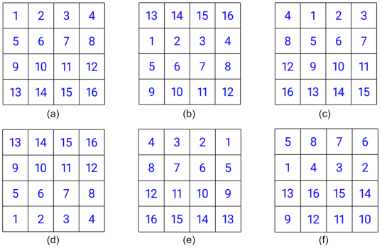
Figure 6: Under the local reversible transformations $(\mathcal{LR}_{box})$, the arrangement of the numbers (associated with the product effect) in Table 3 get modified. Here we show few examples: (a) $\mathbb{I}_{A}\otimes\mathbb{I}_{B}$, (b) $r_{A}\otimes\mathbb{I}_{B}$, (c) $\mathbb{I}_{A}\otimes r_{B}$, (d) $f_{A}\otimes\mathbb{I}_{B}$, (e) $\mathbb{I}_{A}\otimes f_{B}$, (f) $f_{A}r_{A}^{2}\otimes f_{B}r_{B}^{3}$.

With this notation, if Alice applies the transformation $r_{A}$ on her part then each row in Table 3 steps downward and the last row wraps back to the first row. Similarly, for $r_{B}$ each column shifts one step rightwards and the last column wraps back to the first column. On the other hand, the operations $f_{A}$ reflects the Table 3 about the central horizontal line, i.e. $\mbox{row}-1\leftrightarrow\mbox{row}-4$ and $\mbox{row}-2\leftrightarrow\mbox{row}-3$; and under $f_{B}$ we have $\mbox{column}-1\leftrightarrow\mbox{column}-4$ and $\mbox{column}-2\leftrightarrow\mbox{column}-3$. All other local reversible transformations of the Table 3 can be obtained by suitable combinations of these elementary operation (see Fig.6).

We now move on to calculating the number of orbits. For that, according to Burnside’s Lemma, we need to find the number of fixed points for every local reversible transformation. Consider the transformation $r_{A}f_{A}\otimes\mathbb{I}_{B}$. As shown in Fig.7, the set of effects $\{1,2,3,4,9,10,11,12\}$ remain fixed under this transformation, whereas the pairs $\{5,13\}$,$\{6,14\}$,$\{7,15\}$ and $\{8,16\}$ exchange places among themselves. In order to find the number of fixed points of $r_{A}f_{A}\otimes\mathbb{I}_{B}$ we need to choose a set of $8$ effects that remains invariant under the action of $r_{A}f_{A}\otimes\mathbb{I}_{B}$. We have the following possibilities:

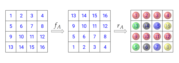
Figure 7: (Color online) The effects colored red remain fixed under the action of $r_{A}f_{A}\otimes\mathbb{I}_{B}$. The effects colored green $\{5,13\}$ is a pair of effects which flip to each other upon action of $r_{A}f_{A}\otimes\mathbb{I}_{B}$. Similarly, the black pair $\{6,14\}$, the blue pair $\{7,15\}$, and the yellow pair $\{8,16\}$ flip to each other under action of $r_{A}f_{A}\otimes\mathbb{I}_{B}$.

• choose all the fixed $8$ effects $\implies^{8}C_{8}\times^{4}C_{0}$ possibilities,

• choose $6$ fixed effects and $1$ pair $\implies^{8}C_{6}\times^{4}C_{1}$ possibilities,

• choose $4$ fixed effects and $2$ pairs $\implies^{8}C_{4}\times^{4}C_{2}$ possibilities,

• choose $2$ fixed effects and $3$ pairs $\implies^{8}C_{2}\times^{4}C_{3}$ possibilities,

• choose all $4$ pairs $\implies^{8}C_{0}\times^{4}C_{4}$ possibilities,

Therefore we have total $646$ different fixed points for $r_{A}f_{A}\otimes\mathbb{I}_{B}$. For the other group elements in $\mathcal{LR}_{box}$ we can carry a similar procedure to count the number of fixed points, which has been shown in Table 4.

$\otimes$	$\mathbb{I}_{B}$	$r_{B}$	$r^{2}_{B}$	$r^{3}_{B}$	$f_{B}$	$r_{B}f_{B}$	$r^{2}_{B}f_{B}$	$r^{3}_{B}f_{B}$
$\mathbb{I}_{A}$	$12870$	$6$	$70$	$6$	$70$	$646$	$70$	$646$
$r_{A}$	$6$	$6$	$6$	$6$	$6$	$6$	$6$	$6$
$r^{2}_{A}$	$70$	$6$	$70$	$6$	$70$	$70$	$70$	$70$
$r^{3}_{A}$	$6$	$6$	$6$	$6$	$6$	$6$	$6$	$6$
$f_{A}$	$70$	$6$	$70$	$6$	$70$	$70$	$70$	$70$
$r_{A}f_{A}$	$646$	$6$	$70$	$6$	$70$	$150$	$70$	$150$
$r^{2}_{A}f_{A}$	$70$	$6$	$70$	$6$	$70$	$70$	$70$	$70$
$r^{3}_{A}f_{A}$	$646$	$6$	$70$	$6$	$70$	$150$	$70$	$150$

Table 4: Number of fixed point for all the local reversible transformations $g=t_{A}\otimes t_{B}\in\mathcal{LR}_{box}.$

Thus from Table 4 we have the total number of orbits which turns out to be

# of orbits $$=\frac{1}{|\mathcal{LR}_{box}|}\sum_{g\in\mathcal{LR}_{box}}\mbox{\# of fixed points of $g$}$$

$$=\frac{1}{64}\times\mbox{(sum of all entries in Table \ref{tab4})}$$

$$=\frac{18112}{64}=283.$$

Following a similar counting procedure for higher gons, we obtain Table 2.

References

- [1] R. Horodecki, P. Horodecki, M. Horodecki, and K. Horodecki; Quantum entanglement, Rev. Mod. Phys. 81, 865 (2009).
- [2] J.S. Bell; On the Einstein Podolsky Rosen paradox, Physics 1, 195 (1964).
- [3] J. S. Bell; On the Problem of Hidden Variables in Quantum Mechanics, Rev. Mod. Phys. 38, 447 (1966).
- [4] N. D. Mermin; Hidden variables and the two theorems of John Bell, Rev. Mod. Phys. 65, 803 (1993).
- [5] N. Brunner, D. Cavalcanti, S. Pironio, V. Scarani, and S. Wehner; Bell nonlocality, Rev. Mod. Phys. 86, 419 (2014).
- [6] J. F. Clauser, M.l A. Horne, A. Shimony, and R. A. Holt; Proposed Experiment to Test Local Hidden-Variable Theories, Phys. Rev. Lett. 24, 549 (1970).
- [7] B. S.Cirel’son; Quantum generalizations of Bell’s inequality, Lett Math Phys 4, 93–100 (1980).
- [8] A. Acín, S. Massar, and S. Pironio; Randomness versus Nonlocality and Entanglement, Phys. Rev. Lett. 108, 100402 (2012).
- [9] A. Coladangelo, K. Goh and V. Scarani; All pure bipartite entangled states can be self-tested, Nat Commun 8, 15485 (2017).
- [10] L. Hardy; Nonlocality for two particles without inequalities for almost all entangled states, Phys. Rev. Lett. 71, 1665 (1993).
- [11] S. Goldstein; Nonlocality without inequalities for almost all entangled states for two particles, Phys. Rev. Lett. 72, 1951 (1994).
- [12] G. Kar; Hardy’s nonlocality for mixed states, Phys. Lett. A 228, 119 (1997).
- [13] M. Banik, S. S. Bhattacharya, N. Ganguly, T. Guha, A. Mukherjee, A. Rai and A. Roy; Two-Qubit Pure Entanglement as Optimal Social Welfare Resource in Bayesian Game, Quantum 3, 185 (2019).
- [14] P. Janotta, C. Gogolin, J. Barrett, and N. Brunner; Limits on nonlocal correlations from the structure of the local state space, New J. Phys. 13, 063024 (2011).
- [15] P. Janotta and H. Hinrichsen; Generalized probability theories: what determines the structure of quantum theory? J. Phys. A: Math. Theor. 47, 323001 (2014).
- [16] N. Brunner, M. Kaplan, A. Leverrier and P. Skrzypczyk; Dimension of physical systems, information processing, and thermodynamics, New J. Phys. 16, 123050 (2014).
- [17] M. Banik, S. Saha, T. Guha, S. Agrawal, S. S. Bhattacharya, A. Roy, and A. S. Majumdar; Constraining the state space in any physical theory with the principle of information symmetry, Phys. Rev. A 100, 060101(R) (2019).
- [18] S. S. Bhattacharya, S. Saha, T. Guha, and M. Banik; Nonlocality without entanglement: Quantum theory and beyond, Phys. Rev. Research 2, 012068(R) (2020).
- [19] S. Saha, T. Guha, S. S. Bhattacharya, and M. Banik; Distributed Computing Model: Classical vs. Quantum vs. Post-Quantum, arXiv:2012.05781 [quant-ph].
- [20] S. Popescu and D. Rohrlich; Quantum nonlocality as an axiom, Found. Phys. 24, 379 (1994).
- [21] G. W. Mackey; Mathematical Foundations of Quantum Mechanics; New York (1963); Dover reprint (2004).
- [22] G. Ludwig, Attempt of an axiomatic foundation of quantum mechanics and more general theories II, III, Commun. Math. Phys. 4, 331 (1967); Commun. Math. Phys. 9, 1 (1968).
- [23] B. Mielnik, Geometry of quantum states, Commun. Math. Phys. 9, 55 (1968).
- [24] L. Hardy; Quantum Theory From Five Reasonable Axioms, arXiv:quant-ph/0101012.
- [25] J. Barrett; Information processing in generalized probabilistic theories, Phys. Rev. A 75, 032304 (2007).
- [26] G. Chiribella, G. Mauro D’Ariano, and P. Perinotti; Probabilistic theories with purification, Phys. Rev. A 81, 062348 (2010).
- [27] H. Barnum and A. Wilce; Information Processing in Convex Operational Theories, Electronic Notes in Theoretical Computer Science (ENTCS) 270, 3 (2011).
- [28] G. Chiribella, G. M. D’Ariano, and P. Perinotti; Informational derivation of quantum theory, Phys. Rev. A 84, 012311 (2011).
- [29] I. Namioka and R. R. Phelps; Tensor products of compact convex sets, Pac. J. Math. 31, 469 (1969).
- [30] M. P. Müller and C. Ududec; Structure of Reversible Computation Determines the Self-Duality of Quantum Theory, Phys. Rev. Lett. 108, 130401 (2012).
- [31] S. Massar and M. K. Patra; Information and communication in polygon theories, Phys. Rev. A 89, 052124 (2014).
- [32] S. W. Al-Safi and J. Richens; Reversibility and the structure of the local state space, New J. Phys. 17, 123001 (2015).
- [33] S. Saha, S. S. Bhattacharya, T. Guha, S. Halder, and M. Banik; Advantage of Quantum Theory over Nonclassical Models of Communication, Annalen der Physik 532, 2000334 (2020).
- [34] R. K. Patra, S. G. Naik, E. P. Lobo, S. Sen, T. Guha, S. S. Bhattacharya, M. Allimuddin, and M. Banik; Classical superdense coding and communication advantage of a single quantum, arXiv:2202.06796 [quant-ph].
- [35] K. P. Seshadreesan and S. Ghosh, Constancy of maximal nonlocal probability in Hardy’s nonlocality test for bipartite quantum systems, J. Phys. A: Math. Theor. 44, 315305 (2011).
- [36] R. Rabelo, L. Y. Zhi, and V. Scarani; Device-Independent Bounds for Hardy’s Experiment, Phys. Rev. Lett. 109, 180401 (2012).
- [37] S. Das, M. Banik, A. Rai, MD R. Gazi, and S. Kunkri; Hardy’s nonlocality argument as a witness for postquantum correlations, Phys. Rev. A 87, 012112 (2013).
- [38] S. Das, M. Banik, Md. R. Gazi, A. Rai and S. Kunkri; Local orthogonality provides a tight upper bound for Hardy’s nonlocality, Phys. Rev. A 88, 062101 (2013).
- [39] S. Das, M. Banik, Md. R. Gazi, A. Rai, S. Kunkri and R. Rahaman; Bound on tri-partite Hardy’s nonlocality respecting all bi-partite principles, Quan. Inf. Processing 12, 3033 (2013).
- [40] R. Ramanathan et al. Practical No-Signalling proof Randomness Amplification using Hardy paradoxes and its experimental implementation, arXiv:1810.11648 [quant-ph].
- [41] A. Rai, M. Pivoluska, M. Plesch, S. Sasmal, M. Banik, and S. Ghosh; Device-independent bounds from Cabello’s nonlocality argument, Phys. Rev. A 103, 062219 (2021).
- [42] A. Rai, M. Pivoluska, S. Sasmal, M. Banik, S. Ghosh, M. Plesch; Self-testing quantum states via nonmaximal violation in Hardy’s test of nonlocality, Phys. Rev. A 105, 052227 (2022).
- [43] M. Dall’Arno, S. Brandsen, A. Tosini, F. Buscemi, and V. Vedral; No-Hypersignaling Principle, Phys. Rev. Lett. 119, 020401 (2017).
- [44] A. Fine; Hidden Variables, Joint Probability, and the Bell Inequalities, Phys. Rev. Lett. 48, 291 (1982).
- [45] A. Fine; Joint distributions, quantum correlations, and commuting observables, J. Math. Phys. 23, 1306 (1982).
- [46] M.Navascués, Y. Guryanova, M.Hoban, et al; Almost quantum correlations, Nat Commun 6, 6288 (2015).
- [47] P. Busch; Unsharp reality and joint measurements for spin observables, Phys. Rev. D 33, 2253 (1986).
- [48] G. Kar; S. Ghosh; S. Choudhary; and M. Banik; Role of Measurement Incompatibility and Uncertainty in Determining Nonlocality, Mathematics 4, 52 (2016).
- [49] N. Gisin; Bell’s inequality holds for all non-product states, Phys. Lett. A 154, 201 (1991).
- [50] R. F. Werner; Quantum states with Einstein-Podolsky-Rosen correlations admitting a hidden-variable model, Phys. Rev. A 40, 4277 (1989).
- [51] J. Barrett; Nonsequential positive-operator-valued measurements on entangled mixed states do not always violate a Bell inequality, Phys. Rev. A 65, 042302 (2002).
- [52] A. Rai, MD. R. Gazi, M. Banik, S. Das, and S. Kunkri; Local simulation of singlet statistics for restricted set of measurement, J. Phys. A: Math. Theor. 45, 475302 (2012).
- [53] A. Peres; Separability Criterion for Density Matrices, Phys. Rev. Lett. 77, 1413 (1996).
- [54] M. Horodecki, P. Horodecki, and R. Horodecki; Separability of mixed states: necessary and sufficient conditions, Phys. Lett. A 223, 1 (1996).
- [55] E. P. Lobo, S. G. Naik, S. Sen, R. K. Patra, M. Banik, and M. Alimuddin; Local Quantum Measurement Demands Type-Sensitive Information Principles for Global Correlations, arXiv:2111.04002 [quant-ph].
- [56] S. G. Naik, E. P. Lobo, S. Sen, R. K. Patra, M. Alimuddin, T. Guha, S. S. Bhattacharya, and M. Banik; Composition of multipartite quantum systems: perspective from time-like paradigm, Phys. Rev. Lett. 128, 140401 (2022).
- [57] W. Burnside; Theory of Groups of Finite Order, Cambridge University Press (2012).