Recurrent Encoder-Decoder Networks for Vessel Trajectory Prediction with Uncertainty Estimation

Abstract

Recent deep learning methods for vessel trajectory prediction are able to learn complex maritime patterns from historical Automatic Identification System (AIS) data and accurately predict sequences of future vessel positions with a prediction horizon of several hours. However, in maritime surveillance applications, reliably quantifying the prediction uncertainty can be as important as obtaining high accuracy. This paper extends deep learning frameworks for trajectory prediction tasks by exploring how recurrent encoder-decoder neural networks can be tasked not only to predict but also to yield a corresponding prediction uncertainty via Bayesian modeling of epistemic and aleatoric uncertainties. We compare the prediction performance of two different models based on labeled or unlabeled input data to highlight how uncertainty quantification and accuracy can be improved by using, if available, additional information on the intention of the ship (e.g., its planned destination).

I Introduction

Trajectory prediction – for collision avoidance, anomaly detection and risk assessment – is a crucial functional component of intelligent maritime surveillance systems and next-generation autonomous ships. Maritime surveillance systems are increasingly relying on the huge amount of data made available by terrestrial and satellite networks of Automatic Identification System (AIS) receivers. The availability of maritime big data enables the automatic extraction of spatial-temporal mobility patterns that can be processed by modern deep learning networks to enhance trajectory forecasting.

Today, most commercial systems primarily rely on trajectory prediction methods based on the Nearly Constant Velocity (NCV) model, since this linear model is simple, fast, and of practical operability to perform short-term predictions of straight-line trajectories [1]. However, the NCV model tends to overestimate the actual uncertainty as the prediction horizon increases. A novel linear model, based on the Ornstein-Uhlenbeck (OU) stochastic process, is becoming recognized as a reliable means to improve long-term predictions [2], with special focus on uncertainty reduction via estimation of current navigation settings.

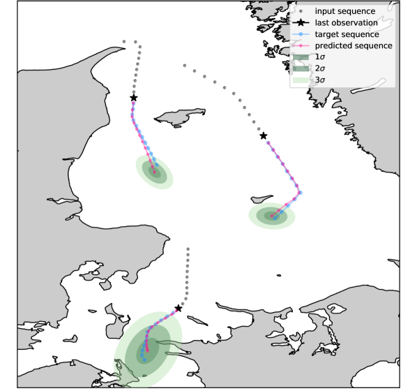
Figure 1: Vessel trajectory prediction with representation of the prediction uncertainty depicted as confidence ellipses (at different confidence levels). Contains data from the Danish Maritime Authority that is used in accordance with the conditions for the use of Danish public data [3].

Although most maritime traffic is very regular, and thus model-based methods can be easily applied, in the presence of maneuvering behaviors of the ship such models will tend to lack the desired prediction accuracy. In such cases, nonlinear and data-driven methods including adaptive kernel density estimation [4], nonlinear filtering [5, 6], nearest-neighbor search methods [7, 8], and machine learning techniques [9], may provide more suitable solutions. Furthermore, the latest advances in deep learning-based predictive models and the combined availability of large volumes of AIS data allow for enhanced vessel trajectory prediction and maritime surveillance. Recent approaches based on deep learning are documented in [10, 11, 12, 13, 14, 15, 16, 17]. However, standard deep learning models cannot provide predictive uncertainty, hence no quantification of the confidence with which the prediction outputs can be trusted is available.

To accompany results from deep learning by their associated confidence levels has recently arisen to be of heightened importance, and naturally there has been significant research attention toward that goal. Data-driven methods for uncertainty quantification have been recently proposed to estimate model and data uncertainty based on ensemble [18] or Bayesian [19, 20, 21, 22, 23] learning. Bayesian deep learning methods apply Bayesian modeling and variational inference to neural networks, leading to Bayesian neural networks (BNNs) that treat the network parameters as random variables instead of deterministic unknowns to represent the model uncertainty on its predictions. BNNs can capture the uncertainty within the learning model, while maintaining the flexibility of deep neural networks, and hence they are particularly appealing for safety-critical applications (e.g., autonomous transportation systems, robotics, medical and space systems) where uncertainty estimates can be propagated in an end-to-end neural architecture to enable improved decision making. In particular, [19] shows that dropout, a well-known regularization technique to prevent neural network over-fitting [24], can be used as a variational Bayesian approximation of the predictive uncertainty in existing deep learning models trained with standard dropout, by performing Monte Carlo (MC) sampling with dropout at test time, i.e., by sampling the network with random omission of units representing MC samples obtained from the posterior distribution over models. In [20] a Bayesian deep learning approach for the combined quantification of both data and model uncertainty, extracted from BNNs, is proposed for computer vision applications. In addition, a neural network architecture based on Long Short-Term Memory (LSTM) with uncertainty modeling is proposed in [25] to incorporate non-Markovian dynamic models in the prediction step of a standard Kalman filter for target tracking.

In this paper, we present a vessel trajectory learning and prediction framework to generate future vessel trajectory samples given the sequence of the latest AIS observations. The proposed method is built upon the LSTM encoder-decoder architecture presented in [16, 17], which has emerged as an effective and scalable model for sequence-to-sequence learning of maritime trajectories. We extend [16, 17] by providing a practical quantification of the predictive uncertainty via Bayesian learning tools based on MC dropout [19]. Preliminary work on trajectory prediction with uncertainty quantification applied to the maritime domain was presented in [26].

In this work, we extend [26] by providing a comprehensive description of the prediction uncertainty modeling, a detailed introduction of the variational LSTM model used to implement our encoder-decoder architecture, and by proposing an alternative decoder scheme with a novel regularization method of the information about the vessel’s intention, which may be available in the maritime surveillance data. Moreover, we present novel results on the estimated predicted variance, and a performance comparison demonstrating the gain in state prediction accuracy with respect to [26]. Fig. 1 shows an example of how the proposed model is able to predict future trajectories and prediction uncertainty given input sequences from past data.

To summarize, the main contributions of this work are:

1. A model for the aleatoric and epistemic uncertainty of trajectory predictions provided by encoder-decoder RNNs using Bayesian deep learning tools;

2. A novel regularization method for the decoding phase to prevent complex co-adaptations between the encoded data and the high-level information about the vessel’s intention;

3. Experimental results on real-world AIS data showing the effectiveness of the proposed encoder-decoder architecture with uncertainty modeling in learning trajectory predictions with well-quantified uncertainty estimates using labeled and unlabeled data.

The paper is organized as follows. In Section II, we introduce the vessel trajectory prediction problem. In Section III, we present the proposed attention-based encoder-decoder framework for trajectory prediction with uncertainty. Experimental results on a real-world AIS dataset are presented and discussed in Section IV. Finally, we conclude the paper in Section V.

II Problem formulation

We formulate the vessel trajectory prediction problem as a supervised learning process by following a sequence-to-sequence deep learning approach to directly generate the distribution of an output sequence of future states given an input sequence of past AIS observations. From a probabilistic perspective, the objective is to determine the following predictive distribution

$$p(\mathbf{y}_{1:h}^{*}|\mathbf{x}_{1:\ell}^{*},\mathcal{D}),$$ (1)

which represents the probability of an output sequence $\mathbf{y}_{1:h}^{*}\triangleq\{\mathbf{s}_{k}\}_{k=1}^{h}\in\mathbb{R}^{d\times h}$ of $h\geq 1$ future $d$-dimensional states of the vessel given a new input sequence $\mathbf{x}_{1:\ell}^{*}\triangleq\{\mathbf{s}_{k}\}_{k=1}^{\ell}\in\mathbb{R}^{d\times\ell}$ of $\ell\geq 1$ observed states, and the available training data $\mathcal{D}=\{\mathcal{X}^{i},\mathcal{Y}^{i},\Psi^{i}\}_{i=1}^{N}$ containing the two sets $\mathcal{X}^{i}=\{\mathbf{x}_{1:\ell}^{i}\}_{i=1}^{N}$ and $\mathcal{Y}^{i}=\{\mathbf{y}_{1:h}^{i}\}_{i=1}^{N}$ of training input and, respectively, output sequences. Note that each sequence element $\mathbf{s}^{i}_{k}\triangleq\mathbf{s}^{i}(t_{k})\in\mathbb{R}^{d}$ represents the vessel’s position in latitude and longitude coordinates, taken from the available time-stamped AIS messages. In many practical cases, it is also possible to exploit some additional information available from AIS data such as the vessel destination. The destination port is an example of voyage related information provided by the AIS that may be relevant to anticipate a vessel trajectory. We denote this (possibly available) input feature, which may be salient to predict the $i$-th output sequence, by $\Psi^{i}=\{\bm{\psi}^{i}\}_{i=1}^{N}$, where $\bm{\psi}^{i}\in\{0,1\}^{v}$ is the $v$-way categorical feature for each trajectory $i$ representing the class label of the specific motion pattern encoded into a one-hot vector of size $v$[17]. For example, $\bm{\psi}^{i}=\{0,0,1\}$ would mean that this particular vessel followed a trajectory that has been labeled $\#3$ based on three possible destinations.

II-A Modeling prediction uncertainty

Uncertainty on the prediction estimates can be captured with recently developed Bayesian deep learning tools, which offer a practical framework for representing uncertainty in deep learning models [20, 21, 22]. In the context of supervised learning, two forms of uncertainty, i.e., aleatoric and epistemic uncertainty are considered, where epistemic is the reducible and aleatoric the irreducible part of uncertainty [20]. Aleatoric (or data) uncertainty captures noise inherent in the observations, whereas epistemic (or model) uncertainty accounts for uncertainty in the neural network model parameters [20]. Epistemic uncertainty is a particular concern for neural networks given their many free parameters, and can be large for data that is significantly different from the training set. Thus, for any real-world application of neural network uncertainty estimation, it is critical that it be taken into account. We follow a combined aleatoric-epistemic model [20] to capture both aleatoric and epistemic uncertainty in our prediction model.

Following a Bayesian framework [27] with prior distributions placed over the parameters of the NN, epistemic uncertainty can be captured by learning a distribution of NN models $p(F|\mathcal{D})$ representing the posterior distribution over the space of functions $\mathbf{y}_{1:h}=F(\mathbf{x}_{1:\ell})$ that are likely to have generated our dataset $\mathcal{D}$. The predictive probability (1) is then obtained by marginalizing over the implied posterior distribution of models, i.e.,

$$p(\mathbf{y}_{1:h}^{*}|\mathbf{x}_{1:\ell}^{*},\mathcal{D})=\int p(\mathbf{y}_{1:h}^{*}|\mathbf{x}_{1:\ell}^{*},F)p(F|\mathcal{D})dF.$$ (2)

In our case, $F$ are RNN encoder-decoder models [17] assumed to be described by a finite set of parameters $\bm{\theta}$, such that

$$p(\mathbf{y}_{1:h}^{*}|\mathbf{x}_{1:\ell}^{*},\mathcal{D})=\int p(\mathbf{y}_{1:h}^{*}|\mathbf{x}_{1:\ell}^{*},\bm{\theta})p(\bm{\theta}|\mathcal{D})d\bm{\theta}.$$ (3)

Since $p(\bm{\theta}|\mathcal{D})$ cannot be obtained analytically, it can be approximated by using variational inference with approximating distribution $q(\bm{\theta})$, which allows for efficient sampling. This results in the approximate predictive distribution

$$q(\mathbf{y}_{1:h}^{*}|\mathbf{x}_{1:\ell}^{*},\mathcal{D})=\int p(\mathbf{y}_{1:h}^{*}|\mathbf{x}_{1:\ell}^{*},\bm{\theta})q(\bm{\theta})d\bm{\theta},$$ (4)

which can be kept as close as possible to the original distribution by minimizing the Kullback-Leibler (KL) divergence between $q(\bm{\theta})$ and the true posterior $p(\bm{\theta}|\mathcal{D})$ during the training stage.

Let us consider a generic NN architecture with $L$ transformation layers, and denote by $\mathbf{W}_{l}$ the weight matrix of size $K_{l}\times K_{l-1}$ for each layer $l=1,\dots,L$. Then, following [28], by setting the set of weight matrices of the NN architecture as the set of parameters, i.e., $\bm{\theta}=\{\mathbf{W}_{l}\}_{l=1}^{L}$, and by using a Bernoulli approximating variational distribution, it is possible to relate variational inference in Bayesian NNs to the dropout mechanism. In particular, the approximating distribution can be defined for each row $i$ of $\mathbf{W}_{l}$ as

$$q(\mathbf{w}_{i})=\gamma\,\mathcal{N}(\mathbf{w}_{i};\mathbf{0},\rho^{2}\mathbf{I})+(1-\gamma)\mathcal{N}(\mathbf{w}_{i};\mathbf{m}_{i},\rho^{2}\mathbf{I}),$$ (5)

where $\mathbf{m}_{i}$ is the vector of variational parameters, $\rho$ the standard deviation of the Gaussian prior distribution placed over $\mathbf{w}_{i}$, and $\gamma$ the Bernoulli probability used for dropout. Then, evaluating the model output $F_{\widehat{\bm{\theta}}}$ where sample $\widehat{\bm{\theta}}\sim q({\bm{\theta}})$ corresponds to performing dropout by randomly masking rows in the weight matrix $\mathbf{W}_{l}$ during the forward pass. Predictions can then be obtained by performing MC dropout [19] which consists of executing dropout at test time and averaging results for all $M$ samples, i.e., by approximating (4) as

$$q(\mathbf{y}_{1:h}^{*}|\mathbf{x}_{1:\ell}^{*},\mathcal{D})\approx\frac{1}{M}\sum_{j=1}^{M}p(\mathbf{y}_{1:h}^{*}|\mathbf{x}_{1:\ell}^{*},\widehat{\bm{\theta}}_{j}),$$ (6)

with $\widehat{\bm{\theta}}_{j}\sim q({\bm{\theta}})$. Note that in the case of MC dropout for RNNs, the same parameter realizations $\widehat{\bm{\theta}}_{j}$ are used for each time step of the input sequence [28].

As shown in [20], aleatoric uncertainty can be modeled together with epistemic uncertainty by estimating the sufficient statistics of a given distribution describing the measurement noise of data. By fixing a Gaussian likelihood to model aleatoric uncertainty the predictive distribution of an output sequence $\hat{\mathbf{y}}_{1:h}$ for a given input sequence $\mathbf{x}_{1:\ell}$ can be approximated by a sequence of multivariate Gaussian distributions where each output is a Gaussian $\mathcal{N}(\mathbf{y}_{k};\hat{\mathbf{y}}_{k},\bm{\Sigma}_{k})$ with predictive mean $\hat{\mathbf{y}}_{k}$ and covariance $\bm{\Sigma}_{k},k=1,\dots,h$.

II-B Aleatoric and epistemic uncertainty

The supervised learning task (1) can be recast as a sequence regression problem [29], which aims at training a neural network model $F$ to predict, given an input sequence $\mathbf{x}_{1:\ell}$ of length $\ell$, the predictive mean $\hat{\mathbf{y}}_{1:h}$ and the predictive covariance $\bm{\Sigma}_{1:h}$, i.e.

$$[\hat{\mathbf{y}}_{1:h},\bm{\Sigma}_{1:h}]=F_{\widehat{\bm{\theta}}}(\mathbf{x}_{1:\ell})$$ (7)

where $F$ is a BNN parameterized by model weights $\widehat{\bm{\theta}}$ drawn from the approximate dropout variational distribution $\widehat{\bm{\theta}}\sim q(\bm{\theta})$. Note that a single network can be used to predict both $\hat{\mathbf{y}}_{1:h}$ and $\bm{\Sigma}_{1:h}$. By setting the distribution modeling aleatoric uncertainty as Gaussian, we induce a minimization objective of the loss function $\mathcal{L}_{1:h}\triangleq\mathcal{L}(\mathbf{y}_{1:h})$, here defined via the negative log-likelihood

$$\mathcal{L}_{1:h}=\sum_{k=1}^{h}\frac{1}{2}(\mathbf{y}_{k}-\hat{\mathbf{y}}_{k})^{T}\bm{\Sigma}_{k}^{-1}(\mathbf{y}_{k}-\hat{\mathbf{y}}_{k})+\frac{1}{2}\operatorname{ln}|\bm{\Sigma}_{k}|$$ (8)

which enables simultaneous training of both $\hat{\mathbf{y}}_{k}$ and $\bm{\Sigma}_{k}$ in an end-to-end optimization process of the entire vessel prediction and uncertainty estimation framework. Thus, for each state of the predicted sequence, the network outputs a Gaussian distribution parameterized by $\hat{\mathbf{y}}_{k}$ and $\bm{\Sigma}_{k}$ such that the negative log-likelihood in (8) of the ground truth vessel positions $\mathbf{y}_{k},k=1,\dots,h$ over all training data is as small as possible.

If the epistemic uncertainty can be estimated through MC dropout [19, 20] from $M$ samples $\{\hat{\mathbf{y}}_{1:h}^{j},\bm{\Sigma}_{1:h}^{j}\}_{j=1}^{M}$, then the total predictive uncertainty for the output $\mathbf{y}_{k}$ can be approximated as follows:

$$\overline{\bm{\Sigma}}_{k}=\frac{1}{M}\sum_{j=1}^{M}\hat{\mathbf{y}}_{k}^{j}\hat{\mathbf{y}}_{k}^{j^{T}}-\Bigg{[}\frac{1}{M}\sum_{j=1}^{M}\hat{\mathbf{y}}_{k}^{j}\frac{1}{M}\sum_{j=1}^{M}\hat{\mathbf{y}}_{k}^{j^{T}}\Bigg{]}$$

$$+\frac{1}{M}\sum_{j=1}^{M}\bm{\Sigma}_{k}^{j},$$ (9)

where the first two terms of the sum correspond to the epistemic uncertainty, and the third corresponds to the aleatoric uncertainty. Finally, we average the uncertainty across time steps $k=1,\dots,h$ to obtain the uncertainty estimate of the complete output sequence.

III Learning to predict under uncertainty

We extend the encoder-decoder architecture based on recurrent networks with attention proposed for vessel trajectory prediction in [16, 17] by providing a practical quantification of the total (i.e., comprising both model and data: epistemic and aleatoric) predictive uncertainty following a Bayesian deep learning approach.

The encoder-decoder architecture consists of an bidirectional encoder RNN that reads a sequence of vessel positions one state at a time encoding the input information into a sequence of hidden states, and a decoder RNN that generates an output sequence of future states step-by-step conditioned on a context representation of the input sequence generated from the encoder’s hidden states through an attention aggregation layer. Moreover, we show that, if available, additional information on the intention of the vessel can be exploited to generate the decoder’s outputs.

The RNN encoder-decoder architecture consists of an encoder model with $\theta_{E}$ parameters and a decoder model with $\theta_{D}$ parameters. Each model is implemented as a fully-trainable RNN containing different weight matrices. We define the Bernoulli variational distribution $q(\theta)$ over the union of all the weight matrices of our architecture, i.e., $\theta=\{\theta_{E},\theta_{D}\}$. In the next sections we will see how the full model learns to predict future trajectories under uncertainty.

III-A Variational LSTM

LSTM networks are a special kind of RNN capable of capturing long temporal patterns in sequential data. They work well on a large variety of problems [17, 16, 30]. A Bayesian view of RNNs has been proposed in [28], where the authors interpret LSTM as probabilistic models considering the network weights as variables trainable by suitable likelihood functions. This has been shown to be equivalent to implementing a novel variant of dropout for RNN models to approximate the posterior distribution over the weights with a mixture of Gaussians leading to a tractable optimization objective.

Following [28], we extend the deterministic LSTM architecture implementing dropout on input or output, and recurrent connections, with the same network units dropped at each time step. In this paper, the LSTM architecture maps the input sequence $\mathbf{x}_{1},\dots,\mathbf{x}_{\ell}$ into a sequence of cell activation and hidden states by applying the tied-weights LSTM parameterization in [28]:

$$\begin{bmatrix}\tilde{\mathbf{i}}_{t}\\ \tilde{\mathbf{f}}_{t}\\ \tilde{\mathbf{o}}_{t}\\ \tilde{\mathbf{g}}_{t}\end{bmatrix}=\underbrace{\begin{bmatrix}\mathbf{W}_{i}&\mathbf{U}_{i}\\ \mathbf{W}_{f}&\mathbf{U}_{f}\\ \mathbf{W}_{o}&\mathbf{U}_{o}\\ \mathbf{W}_{g}&\mathbf{U}_{g}\end{bmatrix}}_{\mathbf{W}_{R}}\begin{bmatrix}\mathbf{x}_{t}\\ \mathbf{h}_{t-1}\end{bmatrix}=\begin{bmatrix}\mathbf{W}_{i}\mathbf{x}_{t}+\mathbf{U}_{i}\mathbf{h}_{t-1}\\ \mathbf{W}_{f}\mathbf{x}_{t}+\mathbf{U}_{f}\mathbf{h}_{t-1}\\ \mathbf{W}_{o}\mathbf{x}_{t}+\mathbf{U}_{o}\mathbf{h}_{t-1}\\ \mathbf{W}_{g}\mathbf{x}_{t}+\mathbf{U}_{g}\mathbf{h}_{t-1}\end{bmatrix},$$ (10)

where $\mathbf{W}_{i},\mathbf{W}_{f},\mathbf{W}_{o},\mathbf{W}_{g}$ are all $p$-by-$d$ weight matrices, and $\mathbf{U}_{i},\mathbf{U}_{f},\mathbf{U}_{o},\mathbf{U}_{g}$ have dimension $p$ by $p$, where $d$ is the number of input features and $p$ is the dimension of the (unidirectional) hidden state, i.e., $\mathbf{h}_{t-1}\in\mathbb{R}^{p}$. The input, forget, output, and input modulation gates are $\mathbf{i}_{t}$, $\mathbf{f}_{t}$, $\mathbf{o}_{t}$ and $\mathbf{g}_{t}$, respectively, and can be computed as

$$\mathbf{i}_{t} = \operatorname{sigm}(\tilde{\mathbf{i}}_{t}),$$ f_t = sigm(~f_t),

$$\mathbf{o}_{t} = \operatorname{sigm}(\tilde{\mathbf{o}}_{t}),$$ g_t = tanh(~g_t). (11)

Finally, the cell activation state and hidden state vectors, respectively $\mathbf{c}_{t}$ and $\mathbf{h}_{t}$, are:

$$\mathbf{c}_{t} = \mathbf{f}_{t}\odot\mathbf{c}_{t-1}+\mathbf{i}_{t}\odot\mathbf{g}_{t}$$

$$\mathbf{h}_{t} = \mathbf{o}_{t}\odot\operatorname{tanh}(\mathbf{c}_{t}),$$ (12)

where $\odot$ denotes the Hadamard product. Note that the matrix $\mathbf{W}_{R}\in\mathbb{R}^{(4p)\times(d+p)}$ is a compact representation of all the weight matrices of the four LSTM gates.

In order to perform approximate variational inference over the weights, we may write the dropout variant of the parameterization in (10) as

$$\begin{bmatrix}\tilde{\mathbf{i}}_{t}\\ \tilde{\mathbf{f}}_{t}\\ \tilde{\mathbf{o}}_{t}\\ \tilde{\mathbf{g}}_{t}\end{bmatrix}=\mathbf{W}_{R}\begin{bmatrix}\mathbf{x}_{t}\odot\mathbf{d}_{x}\\ \mathbf{h}_{t-1}\odot\mathbf{d}_{h}\end{bmatrix}$$ (13)

with $\mathbf{d_{x}}$, $\mathbf{d_{h}}$ random masks repeated at all time steps. In the following sections, we will see how to apply the above Variational LSTM (VarLSTM) model to our trajectory prediction task under uncertainty, using an encoder-decoder RNN architecture.

III-B Encoder Network

The encoder network is designed as a bidirectional RNN [31] to capture and analyze the temporal patterns in vessel trajectory both in the positive and negative time directions simultaneously. Following the encoder architecture used in [17], we use two VarLSTM to encode the input sequence using one model for each time direction.

In our VarLSTM encoder implementation, the dropout mask $\mathbf{d}_{h}$ is applied only to the recurrent connections, therefore it does not perturb the input vessel trajectory. In the end, the trainable parameters are $\bm{\theta}_{E}=\{\overrightarrow{\mathbf{W}}_{R},\overleftarrow{\mathbf{W}}_{R}\}$, one weight matrix for each VarLSTM.

The bidirectional VarLSTM maps the input sequence into two different temporal representations: the forward hidden sequence by iterating the forward layer from $t=1$ to $\ell$, and the backward hidden sequence by iterating the backward layer from $t=\ell$ to $1$. In this way, the encoder network is able to learn long-term patterns in both temporal directions. The output layer of the encoder is then updated into a compact hidden state representation obtained by concatenating the forward and backward hidden states, i.e., $\overleftrightarrow{\mathbf{h}}_{t}=\overrightarrow{\mathbf{h}}_{t}\oplus\overleftarrow{\mathbf{h}}_{t}$ computing the output vectors of the encoder layer $\overleftrightarrow{\mathbf{h}}_{1},\dots,\overleftrightarrow{\mathbf{h}}_{\ell}$ for an input sequence of length $\ell$. Each element $\overleftrightarrow{\mathbf{h}}_{t}$ encodes bidirectional spatio-temporal information of the input sequence extracted from the states of the vessel preceding and following the $t$-th component of the sequence.

III-C Attention-based Decoder Network with Uncertainty

In the proposed architecture, the decoder RNN is trained to learn the following conditional probability

$$p(\mathbf{y}_{1},\dots,\mathbf{y}_{h}|\mathbf{x}_{1},\dots,\mathbf{x}_{\ell})=\prod_{t=1}^{h}p(\mathbf{y}_{t}|\{\mathbf{y}_{1},\dots,\mathbf{y}_{t-1}\},\mathbf{z}_{t},\bm{\psi}),$$ (14)

where each factor in (14) can be modeled by an RNN $D$, with trainable parameters $\bm{\theta}_{D}$, of the form

$$p(\mathbf{y}_{t}|\{\mathbf{y}_{1},\dots,\mathbf{y}_{t-1}\},\mathbf{z}_{t})=D(\hat{\mathbf{y}}_{t-1},\mathbf{s}_{t-1},\mathbf{z}_{t};\bm{\theta}_{D}).$$ (15)

The decoder (15) generates the next kinematic state $\hat{\mathbf{y}}_{t}$ given the context vector $\mathbf{z}_{t}$, the possibly available information on the high-level intention $\bm{\psi}$ of the vessel, the decoder’s hidden state $\mathbf{s}_{t-1}$, and the previous predictions $\hat{\mathbf{y}}_{t-1}$, which are fed back into the model in a recursive fashion as additional inputs to predict further into the future. In addition, (15) is initialized by setting

$$\mathbf{s}_{0}=g(\overrightarrow{\mathbf{h}_{\ell}},\bm{\psi})$$ (16)

to map the last encoder (forward) hidden state and the intention into the initial decoder hidden state $\mathbf{s}_{0}$. Note that, similar to [17], this work partially addresses the multimodal nature of the prediction task with the use of the vessel’s intention (i.e., destination) $\bm{\psi}$. However, different from [17] and as an additional measure to avoid overfitting, here the intention information is used only to initialize the decoder through (16), which in this case takes the form

$$\bm{s}_{0}=\tanh(\mathbf{W}_{\psi}\bm{\eta})$$ (17)

with $\bm{\eta}=\overrightarrow{\mathbf{h}_{\ell}}\oplus\bm{\psi}$, $\mathbf{W}_{\psi}$ being the trainable parameters of the neural network (16).

The attention mechanism [32] is adopted as an intermediate layer between the encoder and the decoder to learn the relationship between the observed and the predicted kinematic states while preserving the spatio-temporal structure of the input. We extend the attention module of [32] implemented in [17] by applying a random dropout mask repeated at all time steps $\mathbf{d}_{a}$ to the input hidden features, previously computed by the encoder network. This is achieved by allowing the context representation to be a set of fixed-size vectors, or context set $\mathbf{z}=\{\mathbf{z}_{t}\}_{t=1}^{\ell}$, where each context vector $\mathbf{z}_{t}$ in (15) can be computed as a weighted sum of the encoded input states, i.e., $\mathbf{z}_{t}=\sum_{j=1}^{\ell}\alpha_{tj}\mathbf{h}_{j}\odot\mathbf{d}_{a},$ where $\alpha_{tj}=\operatorname{exp}(e_{tj})/\sum_{k=1}^{\ell}\operatorname{exp}(e_{tk})$ represents the attention weight, and $e_{tj}=a(\mathbf{s}_{t-1},\mathbf{h}_{j}\odot\mathbf{d}_{a};\mathbf{W}_{a})$ is a variational neural network with parameters $\mathbf{W}_{a}$ and dropout mask $\mathbf{d}_{a}$. The variational attention network is trained jointly with the prediction model to quantify the level of matching between the inputs around position $j$ and the output at position $t$ based on the $j$-th encoded input state $\mathbf{h}_{j}$ and the decoder’s state $\mathbf{s}_{t-1}$ (generating the $t$-th output).

In order to deal with uncertainty, the decoder (15) is implemented as a unidirectional VarLSTM which generates the sequence of future predicted distributions by iterating $\forall t=1,\dots,h$:

$$\bm{c}_{t} = \hat{\mathbf{y}}_{t-1}\oplus\mathbf{z}_{t}$$ (18)

$$\mathbf{s}_{t} = \operatorname{\textit{VarLSTM}}(\bm{c}_{t},\mathbf{s}_{t-1};\mathbf{W}_{R})$$ (19)

$$\hat{\mathbf{y}}_{t} = \mathbf{W}_{\mu}\mathbf{s}_{t}$$ (20)

$$\left[\log b_{11},\log b_{22},b_{21}\right]^{T} = \mathbf{W}_{\Sigma}\mathbf{s}_{t}$$ (21)

where $\hat{\mathbf{y}}_{0}=\mathbf{x}_{\ell}$, $\mathbf{z}_{t}$ is the context vector computed through the attention mechanism, and $\mathbf{W}_{\mu}$, $\mathbf{W}_{\Sigma}$ are trainable parameters of a single neural network mapping the VarLSTM output $\mathbf{s}_{t}$ to the parameters in (20)-(21) used to estimate the predictive uncertainty at time step $t$, here modeled as a multivariate Gaussian distribution $\mathcal{N}(\hat{\mathbf{y}}_{t},\mathbf{\Sigma}_{t})$. Note that, while the predictive mean $\hat{\mathbf{y}}_{t}$ can be directly obtained through (20), to stabilize training and enforce positive-definite predictive covariance matrices, the network (21) is trained to predict the elements of a lower triangular matrix with real and positive diagonal entries $\mathbf{B}=\begin{bmatrix}b_{11}&0\\ b_{21}&b_{22}\end{bmatrix}$, such that

$$\bm{\Sigma}_{t}=\mathbf{B}\mathbf{B}^{T}=\begin{bmatrix}\sigma_{t,x}^{2}&\sigma_{t,x}\sigma_{t,y}\rho_{t}\\ \sigma_{t,x}\sigma_{t,y}\rho_{t}&\sigma_{t,y}^{2}\end{bmatrix}$$ (22)

is guaranteed to be positive definite using the Cholesky decomposition (22). Note that $\sigma_{t,x}$ and $\sigma_{t,y}$ in (22) denote the components of the predictive variance $\sigma_{t}$ along the $x$ and, respectively, $y$ direction. Notice also that in the proposed VarLSTM decoder implementation, the $\mathbf{d}_{h}$ dropout mask is applied only on the recurrent connections.

This end-to-end solution is trained by the stochastic gradient descent algorithm in order to learn an optimal function approximation (7). A decoder (15) with such a recursive structure offers the advantage of being able to handle sequences of arbitrary length. The model consists of a set of trainable parameters $\bm{\theta}_{D}=\{\mathbf{W}_{\psi},\mathbf{W}_{R},\mathbf{W}_{a},\mathbf{W_{\mu}},\mathbf{W}_{\Sigma}\}$ respectively used to model the decoder initialization (17), the unidirectional VarLSTM (19), the attention mechanism, and the output distribution given by (20)-(21).

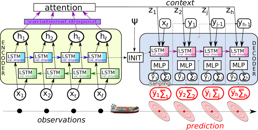
Figure 2: Diagram of the proposed attention-based VarLSTM encoder-decoder architecture for vessel trajectory prediction with uncertainty estimation. The encoder is a bidirectional VarLSTM that maps the input sequence into a sequential hidden state. Then, the encoded information, randomly masked through variational dropout, is passed to an intermediate attention module to generate a context representation of the input. This intermediate representation is fed to the decoder network, implemented as a unidirectional VarLSTM, that generates the sequence of output distributions $\mathcal{N}(\hat{\mathbf{y}}_{t},\mathbf{\Sigma}_{t}),t=1,\dots,h$. Finally, the sequence of total predictive distributions $\mathcal{N}(\overline{\mathbf{y}}_{t},\overline{\mathbf{\Sigma}}_{t})$ is obtained by combining aleatoric and epistemic uncertainty, the latter estimated through MC dropout. Note that the decoder network is initialized using a regularization method on the intention information.

III-D Intention Regularization

Despite the proposed decoder initialization (17), the encoder-decoder architecture may overfit the intention information, and predict erroneous future maneuvers of the vessel. This is due to the fact that the model tends to generate predictions that are mainly based on the high level intention rather than on the information encoded in the past trajectory. To avoid this behavior, and inspired by the dropout mechanism [33], we apply a regularization technique based on dropout noise [34] by randomly masking the intention information at train time in order to prevent complex co-adaptations between the encoded past trajectory and the high-level information.

In particular, we apply a random dropout noise to the intention at each iteration of the training procedure by feeding the intention information $\bm{\psi}$ into (17) with some probability $q$ (a predefined hyperparameter), or setting it to zero otherwise. Thus, the decoder initialization (17) takes the following form

$$\bm{s}_{0}=\tanh(\mathbf{W}_{\psi}(\bm{\eta}\odot\mathbf{d}_{\eta})),\\$$ (23)

where $\mathbf{d}_{\eta}=\frac{p+v}{p}\bm{\nu}$, and $\bm{\nu}\in\{0,1\}^{p+v}$ is a random binary mask on the input information such that $\nu_{i}=1$, $i=1,\dots,p$, and $\nu_{i}=\nu\sim\operatorname{Bern}(1-\gamma)$, $i=p+1,\dots,p+v$. The random variable $\nu$ is Bernoulli with parameter $1-\gamma$, i.e., it takes the value $0$ with probability $\gamma$ for each training sample of the intention components of $\bm{\eta}$, otherwise it is $1$. In other words, this random mask is applied to $\bm{\eta}$ in order to regularize via dropout noise only the intention information $\bm{\psi}\in\{0,1\}^{v}$, while leaving the encoded feature $\overrightarrow{\mathbf{h}_{\ell}}\in\mathbb{R}^{p}$ untouched. Then, a scaling factor $\frac{p+v}{p}$ is applied to the random mask at train time, while leaving the forward pass at test time unchanged. Note that this pre-scaling performed at train time, commonly referred to as the inverted dropout implementation, does not require any changes to the network to compensate for the absence of information during test time, as usually done in traditional dropout [33].

This additional regularization of the intention information can be viewed as a Multimodal Dropout method [35], in which the input features belonging to the same group (or modality) are either all dropped out or all preserved to avoid false co-adaptations between different groups of input information, and to handle missing data in one of the groups at test time. In our case, this has been shown to improve the prediction performance by preventing co-adaptations between the encoded past observations and the possibly available intention information. The improvements in performance with respect to a previous version of the labeled architecture [26] are provided in appendix A for a varying probability $\gamma$.

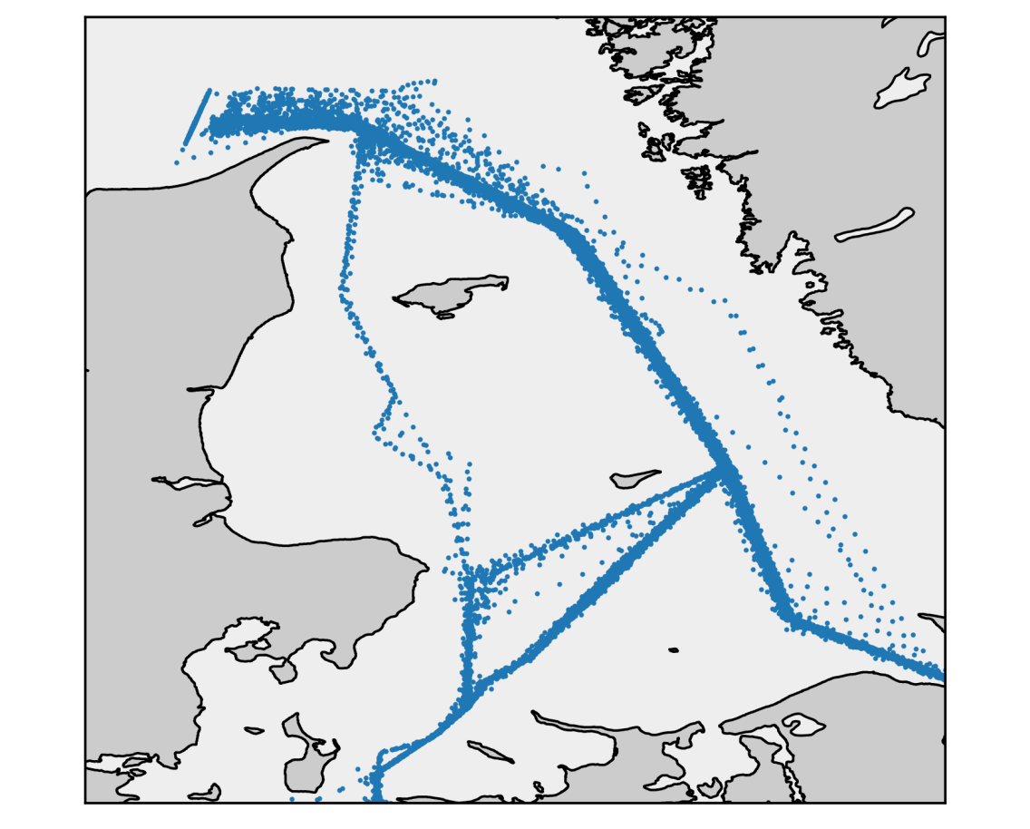
Figure 3: Complete dataset of AIS positions used in the experiments; the training and testing sets are subsets of the dataset showed here. Each dot in the image corresponds to a ship’s position. Contains data from the Danish Maritime Authority that is used in accordance with the conditions for the use of Danish public data [3].

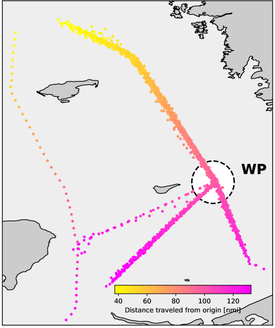
Figure 4: Test dataset used for the evaluation of performance metrics. Each dot in the image corresponds to a ship’s position and is colored based on its distance from a fixed point, located in the upper left corner of the map. Contains data from the Danish Maritime Authority that is used in accordance with the conditions for the use of Danish public data [3].

IV Experiments

In this section we describe the experiments carried out to evaluate the proposed encoder-decoder architecture for trajectory prediction with uncertainty.

IV-A Dataset benchmark

We used an AIS dataset extracted from the historical data made freely available by the Danish Maritime Authority (DMA) [3], comprising $394$ trajectories of tanker vessels belonging to two specific motion patterns of interest in the period ranging from January to February 2020. The complete dataset used in this paper is illustrated in Fig. 3, and a detailed description of the dataset preparation method can be found in [17]. Paths falling into the same maritime pattern are described as sequences of positions in planar coordinates assigned through the Universal Transverse Mercator (UTM) projection (zone 32V), and correlated by voyage-related attributes including departure and destination areas.

In order to provide regular input sequences to train the model in a supervised fashion, we applied a temporal interpolation to each trajectory using a fixed sampling time of $\Delta=15$ minutes to resample the data, and data segmentation by using the sliding window approach to produce fixed-length input and output sequences of length $\ell=h=12$ vessel positions (i.e., $3$ hours).

IV-B Models

We propose an encoder-decoder architecture with attention mechanism composed of a BiLSTM encoder layer with $64$ hidden units, and an LSTM decoder layer with $64$ hidden units. For Bayesian modeling of the epistemic uncertainty, we used MC dropout [19] with $M=100$ samples, and dropout rate applied to recurrent connection $p=0.05$ in both encoder and decoder layers. The model was trained by applying AdamW optimizer [36] with a learning rate of $0.0001$ and weight decay of $0.0001$ to minimize the mean absolute error loss function, an early-stopping rule with $3000$-epoch patience, and a mini-batch size of $200$ samples.

In [4] it is shown how better performance in terms of prediction accuracy can be achieved by labeling the input data based on a high-level pattern information $\bm{\psi}$, such as the vessel’s intended destination. In this regard, we compare the following two different prediction methods based on labeled or unlabeled trajectories, where in the labeled case the neural model is trained to exploit also $\bm{\psi}$.

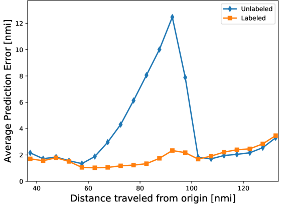
(a)

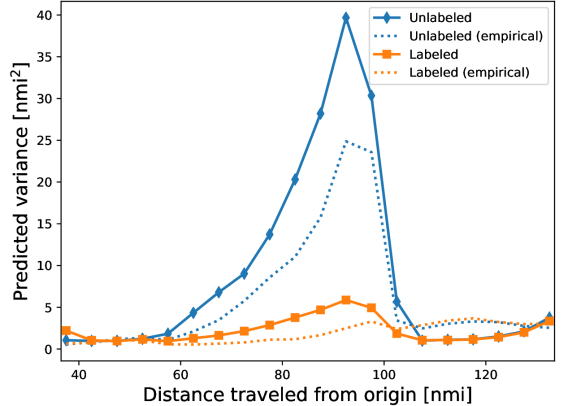
(b)

Figure 5: APE LABEL:sub@fig:compare_dist_perf and predicted total variance LABEL:sub@fig:compare_cov_perf. Both are computed at the $h$-th prediction sample (i.e., prediction horizon 3 hours) and are expressed as a function of the vessel distance from a fixed point, located in the upper left corner of Fig. 4. Panel LABEL:sub@fig:compare_cov_perf shows the square root of the determinant of the covariance matrix produced by the network, which is also known as generalized variance and is proportional to the area of the prediction uncertainty ellipse.

• Unlabeled (U): we train the predictive model and perform prediction using unlabeled data, i.e. using only low-level context representation encoded from a sequence of past observations, without any high-level information about the motion pattern.

• Labeled (L): we train the predictive model and perform prediction using labeled data, i.e. using low-level context representation encoded from a sequence of past observations, as well as additional inputs $\bm{\psi}$ about high-level intention behavior of the vessel. This model includes the intention regularization mechanism with dropout probability $\gamma=0.3$, shown to be the highest-performing model in appendix A.

IV-C Results

In this section we demonstrate the effectiveness of the proposed encoder-decoder VarLSTM in learning trajectory predictions with quantified uncertainty for the maritime domain using labeled and unlabeled data. From the complete dataset in Fig. 3, we isolated a set of trajectories to be used as test set. The selected test trajectories are illustrated in Fig. 4, with a color that changes with the distance traveled from a fixed origin point, located in the upper left corner of the figure. Figure 5a shows the Average Prediction Error (APE) computed as the average Euclidean distance between the predicted position and the ground truth at the $h$-th prediction sample (i.e., prediction horizon 3 hours) as a function of the vessel’s traveled distance from the fixed origin point. This representation allows mapping all prediction errors on a common axis and identifying regions where the prediction error is high.

Figure 5a shows that the two models achieve comparable prediction errors, apart from a specific waypoint area $WP$ (distance between $80$ and $100$ nmi), highlighted in Fig. 4, where the APE obtained with the unlabeled model is much higher than that of the labeled model. This is a crossroad area where vessels can take three different paths towards the same destination, which makes it challenging for the prediction system to anticipate which direction the vessel will follow after the crossroad. The plot proves how high-level information is key to improve prediction performance corresponding to deviation areas (e.g., area $WP$ in Fig. 4). The major difference between unlabeled and labeled predictions is that unlabeled use past observed positions to generate future states, while labeled use additional high-level pattern information, i.e., the ship’s intended destination. In the area $WP$ (Fig. 4), the unavailability of any prior information puts the unlabeled model at a disadvantage for deciding which future path to be followed by the vessel after a crossroad. Instead, the labeled model has more information available, and can generate more realistic future trajectories by exploiting the information related to the pattern descriptor.

In Fig. 5b we show the performance in terms of predictive uncertainty estimation by using the notion of generalized variance, defined as the determinant of the covariance matrix $\overline{\bm{\Sigma}}_{k}$ in (II-B) produced by the unlabeled and labeled models; more precisely, in Fig. 5b, the square root of the determinant of the prediction covariance matrix (averaged over all the trajectories) is plotted, which is proportional to the area of the uncertainty ellipse.

Figure 6 shows the results obtained by the proposed model on a specific trajectory, which intersects the area $WP$ (Fig. 4) at three time steps $k_{i}$, $i=1,2,3$. We perform the predictions considering the sliding window approach, so the input sequence is fed in each neural model to predict the next output sequence. We can see that the predictions using the unlabeled model shown in Figs. 6a–6c detect the correct direction to be followed only after the critical point of a crossroad at time step $k_{3}$, while, conversely, the ones using the labeled model shown in Figs. 6d–6f are able to anticipate the direction to be followed by the vessel after the crossroad many steps ahead. Another important point to be made regarding the predictive uncertainty modeling is how the level of uncertainty quantified by the unlabeled model is larger and includes many possible directions when the path to be taken is still undetermined (e.g., in correspondence to a crossroad such as in Fig. 6b). The dataset used to train the network (represented in Fig. 3) contains multiple paths that can be taken by a vessel after the waypoint; for this reason, the unlabeled model computes a predicted trajectory that is the average mode among multiple possible paths, even if the unimodal prediction is not necessarily a valid future behaviour, and this is especially apparent in Fig. 6b. In contrast, the predictive uncertainty diminishes when the decision of the predictor based on the training data is less complicated due to the direct path of the vessel as shown in Fig. 6c.

In the labeled case, due to the additional high-level information available, the predictions are shown to be more accurate, especially when the vessel is before the crossroad, as showed in Fig. 6d and Fig. 6e. The labeled model can compute more accurate predictions, as some of the possible future paths (specifically, after the waypoint) can be excluded, precisely on the basis of the additional high-level information. This can be easily noted with a comparative inspection of Figures 6b and 6e, where the uncertainty of the unlabeled model, contrary to the labeled one, has to account also for the additional South-East path. It should be noted that the intention information is most useful when it can reduce the multimodal nature of the task to a unimodal prediction task. For instance, in Fig. 6e, the high-level information allows excluding the South-East path, but cannot help further in deciding exactly which one of the two South-West paths the vessel is going to follow. Still, the labeled model achieves better prediction performance, as the additional information allows going from a higher modality prediction task to a lower modality one.

V CONCLUSION

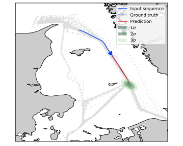
(a)

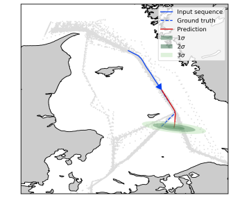
(b)

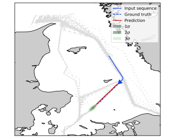
(c)

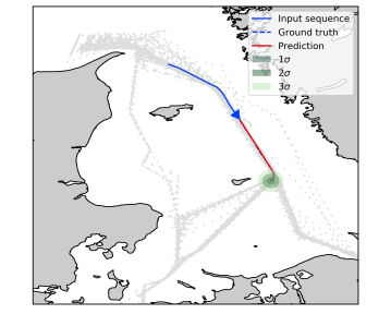
(d)

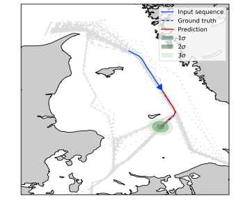
(e)

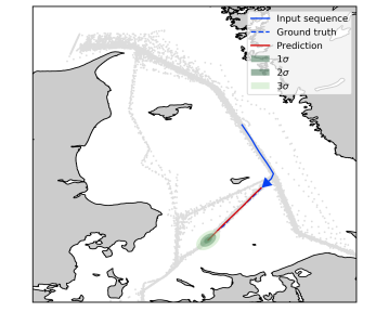
(f)

Figure 6: Predictions computed with unlabeled models LABEL:sub@fig:predictions_unlabeled_1–LABEL:sub@fig:predictions_unlabeled_3 compared to labeled models LABEL:sub@fig:predictions_labeled_1–LABEL:sub@fig:predictions_labeled_3. Contains data from the Danish Maritime Authority that is used in accordance with the conditions for the use of Danish public data [3].

In this paper, we proposed an attention-based recurrent encoder-decoder architecture to address the problem of trajectory prediction with uncertainty quantification applied to a maritime domain case study. The predictive uncertainty is estimated through Bayesian learning by combining both aleatoric and epistemic uncertainty, with the latter modeled via Monte Carlo dropout. Experimental results show that the proposed architecture is able to learn maritime sequential patterns from historical AIS data, and successfully predict future vessel trajectories with a reliable quantification of the predictive uncertainty. Two models are compared and show how prediction performance can be improved by exploiting high-level intention behavior of vessels (e.g., their intended destination) when available. Future lines of research on this topic include the investigation of multimodal prediction techniques in combination with high-level intention modeling to further improve the prediction performance when the intention information alone is not sufficient to fully account for the multimodality of the prediction task.

Appendix A Intention Regularization Performance

In this appendix we investigate how the prediction model can benefit from the intention regularization technique proposed in Section III-D for the novel version of the labeled architecture (Lv2), by comparing the results with those obtained with the previous version of the labeled architecture (Lv1) presented in [26], in which the intention information is injected for each time step during the decoding phase. For this comparison, we used the complete AIS dataset from [17] shown in Fig. 3. In our experiment we split the original dataset composed of $394$ full trajectories into $284$ trajectories for training, $32$ for validation, and $78$ for testing. The windowing procedure proposed in [17] produces $8574$ input/output sequences of length $\ell=h=12$ for training, $1054$ sequences for validation, and $2379$ sequences for the testing phase. In the evaluation of our experiment, we use the APE for different horizons (i.e., 1, 2, and 3 hours), and the Average Displacement Error (ADE) as the average Euclidean distance between the predicted trajectory and the ground truth (i.e., over all the predicted positions of a trajectory) [37, 38]. The performance evaluation of the proposed intention regularization method is shown in Table I, where only the most informative results are shown for a varying probability of intention dropout mask. As shown in Table I, the proposed architecture Lv2 performs better than Lv1, with the best performance achieved by setting $\gamma=0.3$.

TABLE I: Comparison of the impact of intention regularization
on the APE and the ADE metrics

		APE			ADE
Model	Mask ($\gamma$)	1h	2h	3h
Lv1[17]	–	$0.57$	$1.14$	$1.90$	$0.97$
Lv2 (ours)	$0$	$0.56$	$1.11$	$1.86$	$0.95$
Lv2 (ours)	$0.3$	$0.51$	$1.03$	$1.78$	$0.88$
Lv2 (ours)	$0.5$	$0.54$	$1.06$	$1.81$	$0.91$

References

- [1] Z. Xiao, X. Fu, L. Zhang, and R. S. M. Goh, “Traffic pattern mining and forecasting technologies in maritime traffic service networks: A comprehensive survey,” IEEE Trans. Intell. Transp. Syst., vol. 21, no. 5, pp. 1796–1825, 2020.
- [2] L. M. Millefiori, P. Braca, K. Bryan, and P. Willett, “Modeling vessel kinematics using a stochastic mean-reverting process for long-term prediction,” IEEE Trans. Aerosp. Electron. Syst., vol. 52, no. 5, pp. 2313–2330, 2016.
- [3] “Data from the Danish AIS system,” https://www.dma.dk/SikkerhedTilSoes/Sejladsinformation/AIS/Sider/default.aspx, accessed: 2020-07-09.
- [4] B. Ristic, B. La Scala, M. Morelande, and N. Gordon, “Statistical analysis of motion patterns in AIS data: Anomaly detection and motion prediction,” in International Conference on Information Fusion, 2008.
- [5] L. P. Perera, P. Oliveira, and C. Guedes Soares, “Maritime traffic monitoring based on vessel detection, tracking, state estimation, and trajectory prediction,” IEEE Transactions on Intelligent Transportation Systems, vol. 13, no. 3, pp. 1188–1200, 2012.
- [6] F. Mazzarella, V. F. Arguedas, and M. Vespe, “Knowledge-based vessel position prediction using historical AIS data,” in Sensor Data Fusion: Trends, Solutions, Applications, 2015.
- [7] S. Hexeberg, A. L. Flåten, B. H. Eriksen, and E. F. Brekke, “AIS-based vessel trajectory prediction,” in International Conference on Information Fusion, 2017.
- [8] B. R. Dalsnes, S. Hexeberg, A. L. Flåten, B.-O. H. Eriksen, and E. F. Brekke, “The neighbor course distribution method with Gaussian mixture models for AIS-based vessel trajectory prediction,” in International Conference on Information Fusion, 2018, pp. 580–587.
- [9] A. Valsamis, K. Tserpes, D. Zissis, D. Anagnostopoulos, and T. Varvarigou, “Employing traditional machine learning algorithms for big data streams analysis: The case of object trajectory prediction,” Journal of Systems and Software, vol. 127, pp. 249–257, 2017.
- [10] D. Nguyen, R. Vadaine, G. Hajduch, R. Garello, and R. Fablet, “A multi-task deep learning architecture for maritime surveillance using AIS data streams,” IEEE International Conference on Data Science and Advanced Analytics, pp. 331–340, 2018.
- [11] D.-D. Nguyen, C. L. Van, and M. I. Ali, “Vessel trajectory prediction using sequence-to-sequence models over spatial grid,” in ACM International Conference on Distributed and Event-based Systems, 2018, pp. 258–261.
- [12] J. Y. Yu, M. O. Sghaier, and Z. Grabowiecka, “Deep learning approaches for AIS data association in the context of maritime domain awareness,” in International Conference on Information Fusion, 2020.
- [13] X. Zhou, Z. Liu, F. Wang, Y. Xie, and X. Zhang, “Using deep learning to forecast maritime vessel flows,” Sensors, vol. 20, no. 6, 2020.
- [14] B. Murray and L. P. Perera, “A dual linear autoencoder approach for vessel trajectory prediction using historical AIS data,” Ocean Engineering, vol. 209, p. 107478, 2020.
- [15] ——, “An AIS-based deep learning framework for regional ship behavior prediction,” Reliability Engineering & System Safety, 2021.
- [16] N. Forti, L. M. Millefiori, P. Braca, and P. Willett, “Prediction of vessel trajectories from AIS data via sequence-to-sequence recurrent neural networks,” in IEEE International Conference on Acoustics, Speech and Signal Processing, 2020, pp. 8936–8940.
- [17] S. Capobianco, L. M. Millefiori, N. Forti, P. Braca, and P. Willett, “Deep learning methods for vessel trajectory prediction based on recurrent neural networks,” IEEE Trans. Aerosp. Electron. Syst., vol. 57, no. 6, pp. 4329–4346, 2021.
- [18] B. Lakshminarayanan, A. Pritzel, and C. Blundell, “Simple and scalable predictive uncertainty estimation using deep ensembles,” in Advances in Neural Information Processing Systems, vol. 30, 2017.
- [19] Y. Gal and Z. Ghahramani, “Dropout as a Bayesian approximation: Representing model uncertainty in deep learning,” in International Conference on International Conference on Machine Learning (ICML), 2016, pp. 1050–1059.
- [20] A. Kendall and Y. Gal, “What uncertainties do we need in Bayesian deep learning for computer vision?” in Advances in Neural Information Processing Systems, 2017, pp. 5574–5584.
- [21] A. Bhattacharyya, M. Fritz, and B. Schiele, “Long-term on-board prediction of people in traffic scenes under uncertainty,” in IEEE Conference on Computer Vision and Pattern Recognition (CVPR), 2018.
- [22] Y. Xiao and W. Y. Wang, “Quantifying uncertainties in natural language processing tasks,” in Conference on Artificial Intelligence, AAAI, 2019, pp. 7322–7329.
- [23] V. Kuleshov, N. Fenner, and S. Ermon, “Accurate uncertainties for deep learning using calibrated regression,” in International Conference on Machine Learning, vol. 80, 2018, pp. 2801–2809.
- [24] N. Srivastava, G. Hinton, A. Krizhevsky, I. Sutskever, and R. Salakhutdinov, “Dropout: A simple way to prevent neural networks from overfitting,” J. Mach. Learn. Res., vol. 15, no. 1, pp. 1929–1958, 2014.
- [25] S. Jung, I. Schlangen, and A. Charlish, “A mnemonic Kalman filter for non-linear systems with extensive temporal dependencies,” IEEE Signal Processing Letters, vol. 27, pp. 1005–1009, 2020.
- [26] S. Capobianco, N. Forti, L. M. Millefiori, P. Braca, and P. Willett, “Uncertainty-aware recurrent encoder-decoder networks for vessel trajectory prediction,” in IEEE 24th International Conference on Information Fusion (FUSION), 2021.
- [27] R. M. Neal, Bayesian Learning for Neural Networks. Springer-Verlag, 1996.
- [28] Y. Gal and Z. Ghahramani, “A theoretically grounded application of dropout in recurrent neural networks,” in Advances in Neural Information Processing Systems, vol. 29, 2016.
- [29] C. M. Bishop, Neural Networks for Pattern Recognition. USA: Oxford University Press, Inc., 1996.
- [30] A. Graves, A. Mohamed, and G. Hinton, “Speech recognition with deep recurrent neural networks,” in IEEE International Conference on Acoustics, Speech and Signal Processing, 2013, pp. 6645–6649.
- [31] M. Schuster and K. Paliwal, “Bidirectional recurrent neural networks,” Trans. Sig. Proc., vol. 45, no. 11, p. 2673–2681, Nov. 1997.
- [32] D. Bahdanau, K. Cho, and Y. Bengio, “Neural machine translation by jointly learning to align and translate,” in International Conference on Learning Representations, 2015.
- [33] N. Srivastava, G. Hinton, A. Krizhevsky, I. Sutskever, and R. Salakhutdinov, “Dropout: A simple way to prevent neural networks from overfitting,” J. Mach. Learn. Res., vol. 15, no. 1, p. 1929–1958, 2014.
- [34] S. Wager, S. Wang, and P. S. Liang, “Dropout training as adaptive regularization,” in Advances in Neural Information Processing Systems, 2013, p. 351–359.
- [35] N. Neverova, C. Wolf, G. Taylor, and F. Nebout, “ModDrop: Adaptive multi-modal gesture recognition,” IEEE Transactions on Pattern Analysis and Machine Intelligence, vol. 38, no. 8, pp. 1692–1706, 2016.
- [36] I. Loshchilov and F. Hutter, “Decoupled weight decay regularization,” in International Conference on Learning Representations (ICLR), 2019. [Online]. Available: https://arxiv.org/abs/1711.05101
- [37] S. Pellegrini, A. Ess, K. Schindler, and L. V. Gool, “You’ll never walk alone: Modeling social behavior for multi-target tracking,” in IEEE 12th International Conference on Computer Vision, ICCV 2009, Kyoto, Japan, September 27 - October 4, 2009. IEEE Computer Society, 2009, pp. 261–268. [Online]. Available: https://doi.org/10.1109/ICCV.2009.5459260
- [38] A. Alahi, K. Goel, V. Ramanathan, A. Robicquet, L. Fei-Fei, and S. Savarese, “Social LSTM: human trajectory prediction in crowded spaces,” in 2016 IEEE Conference on Computer Vision and Pattern Recognition, CVPR 2016, Las Vegas, NV, USA, June 27-30, 2016. IEEE Computer Society, 2016, pp. 961–971. [Online]. Available: https://doi.org/10.1109/CVPR.2016.110