A Survey on Fairness for Machine Learning on Graphs

Abstract.

Nowadays, the analysis of complex phenomena modeled by graphs plays a crucial role in many real-world application domains where decisions can have a strong societal impact. However, numerous studies and papers have recently revealed that machine learning models could lead to potential disparate treatment between individuals and unfair outcomes. In that context, algorithmic contributions for graph mining are not spared by the problem of fairness and present some specific challenges related to the intrinsic nature of graphs: (1) graph data is non-IID, and this assumption may invalidate many existing studies in fair machine learning, (2) suited metric definitions to assess the different types of fairness with relational data and (3) algorithmic challenge on the difficulty of finding a good trade-off between model accuracy and fairness. This survey is the first one dedicated to fairness for relational data. It aims to present a comprehensive review of state-of-the-art techniques in fairness on graph mining and identify the open challenges and future trends. In particular, we start by presenting several sensible application domains and the associated graph mining tasks with a focus on edge prediction and node classification in the sequel. We also recall the different metrics proposed to evaluate potential bias at different levels of the graph mining process; then we provide a comprehensive overview of recent contributions in the domain of fair machine learning for graphs, that we classify into pre-processing, in-processing and post-processing models. We also propose to describe existing graph data, synthetic and real-world benchmarks. Finally, we present in detail five potential promising directions to advance research in studying algorithmic fairness on graphs. We hope that this survey will motivate researchers to tackle these issues in the near future and believe that it could be attractive to researchers and practitioners in areas including data mining, artificial intelligence and social science. Additional materials, including codes and datasets, to complement this survey are available at: https://github.com/manvic14/Survey_Fairness_Graphs.

1. Introduction

We live in a world where an increasing number of decisions, with major societal consequences, are made or at least supported by algorithms that diligently learn the patterns from a training sample and gain their discriminating ability by identifying the key attributes correlated with the desired output. These attributes, however, can represent sensitive information that, in turn, can lead to a significant bias in model’s predictions when deployed on a previously unseen sample. In today’s technologically advanced world, an increasing number of human tasks are performed or assisted by Machine Learning (ML) algorithms and there is no doubt that the latter will contribute to automating the human decision-making process in more previously uncovered areas too. In this context, an important issue that arises is whether the decisions made or supported by such algorithms are fair.

Several competing and contrasting definitions of fair have been proposed in recent literature. One can broadly categorize these definitions into 1) group fairness, which emphasizes disparate treatment of individuals with respect to some sensitive attribute defining groups. The underlying idea of group fairness is that minority groups should receive similar treatment as that of advantaged groups (Ustun et al., 2019; Hardt et al., 2016a); 2) individual fairness, which requires that similar individuals should be treated similarly (Dwork et al., 2012); and finally 3) counterfactual fairness, where the underlying idea is that a fair decision for a given individual should not depend on the change in the value of his/her sensitive attribute (Kusner et al., 2017).

The problem of biased decision (i.e. unfair situation) in ML can stem from different sources along the decision-making process: the sample data from which the algorithm is learning, the machine learning model used and the exploitation of the output obtained with these models. As a result, contributions in the field of algorithmic fairness can be roughly divided into three categories: the pre-processing methods, whose goal is to remove the bias from the original data itself; the in-processing methods in which the problem of fairness is addressed at the learning time usually by including fairness constraints in the objective function; and the post-processing methods, which aims to remove the bias from the output of the algorithm used to solve the task at hand. These methods are based on various techniques, including but not limited to adversarial learning (Adel et al., 2019; Madras et al., 2018; Xu et al., 2019), causal methods (Nabi and Shpitser, 2018; Glymour and Herington, 2019; Wu et al., 2019b), optimization under constraints (Kim et al., 2018; Celis et al., 2019; Cotter et al., 2019) and sampling methods (Oneto et al., 2019; Dwork et al., 2018). They have been explored in detail in recent surveys (Caton and Haas, 2020; Barocas and Selbst, 2016; Mehrabi et al., 2021) and we refer the interested reader to them for more details but we provide a description of these surveys in Section 2.1. However, while these solutions have proven efficient to mitigate potential bias, they were all designed for tabular data (vectors). In this survey, we are interested in fairness for graph data, or fair graph mining, a recent but fast-growing research area. Graphs present several specificities making difficult to use existing fair approaches, originally developed for standard tabular data. Indeed, graphs are non-iid (independent and identically distributed) and non-euclidean data by nature. The first assumption implies that changing or altering information about a given node (attributes or connections) in the graph will impact its neighbors. As a result, evaluating and mitigating potential bias require proper handling of this assumption. The second assumption implies that before learning any model (classification, ranking or clustering), one should first learn a representation of the graph in the form of vectors. At the node level, this corresponds to node embedding models. And, as we will demonstrate in this survey, depending on the objective function used in these models, the learned node representation can capture different amount of bias, or make it more difficult to mitigate the bias afterward. This last challenge is closely related to the more general problem of fair representation.

Fair Representation Learning

Inducing fairness in machine learning led to the focus on learning fair representations for complex data. The first paper to address this problem (Zemel et al., 2013) proposes an algorithm for fair classification which is capable of both group and individual fairness and, that aims to encode the original information from tabular data while at the same time ignoring the information of the protected group. In the same spirit, adversarial regularization techniques have been proposed to straightforwardly learn fair representations as done by (Madras et al., 2018) and (Edwards and Storkey, 2016). Similarly, in (Creager et al., 2019), authors propose to learn a representation that achieves group and sub-group fairness. Their representations are modifiable at test time both simply and compositionally to achieve sub-group fairness with respect to multiple protected attributes. With similar goal to learn an invariant representation, in (Louizos et al., 2016) the authors propose a semi-supervised fair model based on the Variational Autoencoder (Kingma and Welling, 2014; Rezende et al., 2014) and further guarantee invariance by using a Maximum Mean Discrepancy based regularization (Gretton et al., 2007). Insofar as, to deal with graphs, it is essential to start by learning a representation in a Euclidean space, most of the existing contributions in fair graph mining belong to this family of approaches. These methods are referred to as fair node embeddings and we describe them further in Section 5.

Research Questions

In this survey, we aim to address the three following fundamental research questions about fairness on graphs :

• How can we identify bias in graph-based machine learning? To answer this question, we provide an overview of existing metrics to evaluate bias on graphs and present techniques that have been proposed to reduce bias by transforming the original graph.

• How much of the bias is present in node embedding? Here we are interested in understanding to what extent are some commonly used node embedding techniques transcribing potential bias. This question relates to how to control the bias at training time. We present node embedding methods that include fairness constraints at the learning stage.

• Is the model outcome fair? This last question is linked to the post-processing family of models existing for tabular data, as when reaching this step, we are usually dealing with vectors. We will present existing models that propose to mitigate bias at the task level for graphs.

To cover these questions in a thorough manner, we organize our article as follows. We start by introducing the problem of fairness for graph-related tasks including node embedding, node classification and edge prediction in Section 2. We also present two real-world application cases where unfair graph mining algorithms can lead to discriminatory outcomes. Then, we proceed with a presentation of the existing metrics used to measure and evaluate bias in Section 3, and differentiate based on the level of the graph on which they operate. Sections 4 and 5 presents the main algorithmic contributions for fair graph mining. These sections cover pre-processing approaches that aim to transform the original graph and fair node embedding methods, respectively. Then, in Section 6 we provide an overview of both synthetic and real-world benchmarks that are commonly used to evaluate contributions in fair graph mining. Finally, we conclude this article by discussing some important remaining open challenges in Section 7.

2. Related Work and General Set-up

In this section, we give an overview of existing surveys and tutorials on the topic of fairness in machine learning and graphs. We also define the general framework of fair graph mining and motivate the importance of this research field with two concrete examples.

2.1. Related Surveys and Tutorials

To the best of our knowledge, this survey is the first one dedicated to fairness for graphs. However, we would like to highlight the existence of a tutorial given at CIKM 2021 and entitled Fair Graph Mining(Kang and Tong, 2021). In this tutorial, the authors cover contributions belonging to either group or individual fairness for graphs, before presenting other definitions of fairness, including degree-related fairness and counterfactual fairness. In this survey, we only consider group, individual and counterfactual fairness, as they are the most common forms of fairness studied in this context.

Hereafter, we propose to describe the existing surveys and recurrent tutorials proposed on the broader topic of fairness in machine learning. The first one is an online book (Barocas et al., 2019), where the authors give a very broad overview of the challenges posed by fairness in machine learning. In addition to the more traditional chapters on existing approaches and metrics, they notably provide discussions on the societal aspects of the problem. For instance, on the importance and difficulty of testing discrimination of in-production machine learning systems or the relations between machine learning structural, organizational, and interpersonal discrimination in society. In a similar spirit, in (Beutel et al., 2019), the authors develop a case-study on the application of fairness in machine learning research to a production classification system. This type of study, while not reviewing all existing approaches in the domain, offers interesting new insights on how we can test, measure and address algorithmic fairness in practice. In (Mehrabi et al., 2021), the authors proposed an interesting covering of existing algorithmic methods to achieve fairness in machine learning. The structure and objectives of our survey resemble this last study the most. Finally, recurrent tutorials dedicated to the challenges of fairness in machine learning have been organized over the past few years: among them, we can cite the tutorial on fairness given by Solon Bacrocas and Moritz Hardt at NIPS2017, and the Fairness-Aware Machine Learning: Practical Challenges and Lessons Learned, a tutorial given at KDD 2019 . However we want to emphasis that there is no mention of methods to deal with graphs in the aforementioned references.

2.2. Problem Setup

There exist multiple tasks that we can address when dealing with complex data represented by graphs. We can divide these tasks according to the level of the graph on which they operate: we distinguish graph-level (e.g. predict the property of an entire graph), from node-level (e.g. predict the role of a node or detect communities of nodes within a graph) and edge-level (e.g. predict the existence of an edge) tasks. For mode details about these various tasks, we refer the interest reader to (Aggarwal and Wang, 2010). In this survey, we will focus on node classification and edge prediction. One example of edge-level inference is, given a pair of node, to predict the relationship between them. We can phrase this as an edge-level classification: given a pair of nodes we wish to predict which of these nodes share an edge or what the value of that edge is. For instance, on a social platform, edge prediction amounts to predict potential friendship relation between users. To illustrate the problem of fairness for graphs, we also assume that nodes of the graph can have one or multiple attributes, considered as protected. Thus in the above example, users of the social platform might have entered their gender information. In this context we wish to ensure that the edge prediction will not depend on this factor.

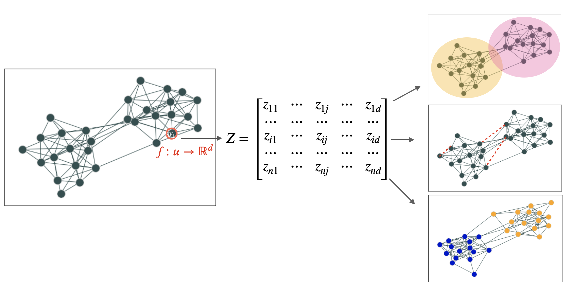
Figure 1. Machine Learning on graphs. From the original graph (left), a mapping function $f$ is learned that produces the matrix of node embeddings $Z$ (middle). These embeddings are then used to solve several types of graphs problems (right): community detection (top), edge prediction (middle) or node classification (bottom).

Notations

Throughout this article, we will use the following notations. Let $\mathbb{V}$ denote an abstract vertex space, and let $\mathcal{V}=\{v_{1},\dots,v_{n}\}\in\mathbb{V}^{n}$ be a set of $n$ vertices drawn from an arbitrary distribution over $\mathbb{V}$. In the finite case, we further consider a graph $\mathcal{G}=(\mathcal{V},\mathcal{E})$ where $\mathcal{E}\subseteq\mathbb{V}\times\mathbb{V}$ defines the set of edges in the graph. Furthermore, we can consider different labels. For edge prediction, we consider $y$ such that a tuple $\{(v_{i},v_{j},y(v_{i},v_{j})\}$ defines the existence (i.e., $y(v_{i},v_{j})=1$) or the absence (i.e., $y(v_{i},v_{j})=0$) of an edge $(i,j)\in\mathcal{E}$ and $m$ is the number of edges in $\mathcal{E}$. Furthermore, we assume the existence of a variable that explicitly encodes some sensitive information, and use the letter $A$ to designate a discrete random variable that captures one or multiple sensitive characteristics. For instance $A(v_{i})=0$ means that the node $v_{i}$ is assigned with the sensitive group labeled as $0$. Note that, one of the main challenges of dealing with such settings, is that the sensitive information might as well be implicitly encoded in the graph structure, requiring to consider this latter when trying to achieve fairness. It can be notably the case in presence of homophily when nodes sharing the same attribute value are more likely to be connected.

Node embedding

As machine learning models typically take tabular data (vectors) as input, for using them on relational data, one needs to add an intermediate step between the original graph representation and the task to be solved. Node embedding consists in learning a (non-)linear mapping of each node $v\in\mathcal{V}$ into a vector space $f:\mathcal{V}\rightarrow\mathbb{R}^{d}$ where $d$ is the number of dimensions of the vector spacce. We further assume that $d\ll n$. These vectorial representations of the nodes are stored in a matrix $\textit{Z}\in\mathbb{R}^{n\times d}$ and referred to as node embeddings. Once learned, these node embeddings can be used for any downstream tasks, including edge prediction, community detection or node classification to name a few, as illustrated in Figure 1. In the context of fair learning, we further expect that these learned node embeddings do not reflect potential bias arising from the original graph, and captured by the sensitive attribute $A$. To sum-up, node embeddings should have the following properties.

1. Embeddings should reflect different properties of the graph structure, e.g, two nodes connected in the graph should have similar embeddings.

2. Embeddings should be independent from one or multiple sensitive attributes, hence one should not be able to retrieve information regarding sensitive attribute from these embeddings.

One should note that having P1 and P2 is rather a difficult task, especially when the structure of the graph is strongly correlated with the protected attribute(s). Consequently, the objective here is usually to find a reasonable trade-off between these properties. Furthermore, while P1 is directly ensured by the objective function used to learn the embeddings, P2 can be obtained in different manners : (1) by pre-processing the original graph to remove potential bias in the data structure before learning the embeddings; (2) by making change, e.g. adding constraints, to the objective function used to learn the embedding; (3) by post-processing the obtained node embeddings to filter out the bias.

Fair Graph Mining

We now describe the three most common tasks that can be solved by using node embeddings as input, namely node classification, edge prediction and community detection. On the one hand, in graphs the nodes are often characterized by contextual information in the form of node attributes. When the values of these attributes (or label) of some nodes are only partially known, node classification or semi supervised label prediction can be used to determine them (Bhagat et al., 2011). Formally, the goal is to learn a function $h:\mathbb{V}\rightarrow y$, where $y$ is a label set. On the other hand, edge prediction considers tuples of nodes as input. Given a pair of nodes, edge prediction consists in determining if an edge exists between them or not. Formally, it aims at finding a function $h:\mathbb{V}\times\mathbb{V}\rightarrow\{0,1\}$ such that $h$ is as close as possible to $y$, the true edge label. These two tasks are supervised, hence the notion of fairness for them is usually defined in terms of the predictions made by the function $h$ conditionally on the protected attributes. As we will see in the next section, different definitions of fairness for supervised tasks have been proposed, and they all capture different aspects of the problem. Finally, community detection consists in discovering cohesive groups or clusters in a complex network. Most of the time, this is done is such a way that nodes belonging to the same community are densely connected to each other while sparsely connected to the rest of the network (Fortunato, 2010). This task is unsupervised and relies less on node embedding (compared with the supervised tasks). However, these methods are often based on properties of the nodes and the graph, such as assortativity or homophily of the graph, that, if exploited can result in more bias (see Section 3). As contributions on fair community detection are more scare, we focus on fair node classification and fair edge prediction in the remaining of this paper.

2.3. Applications

Hereafter, we provide important societal examples of applications where the problem of fairness when dealing with graphs can occur. Note that, this is obviously not an exhaustive list of applications, but these examples motivate us to believe that working on that particular topic is of high importance. We will also use them in the remaining of the article to illustrate some important concepts or intuitions.

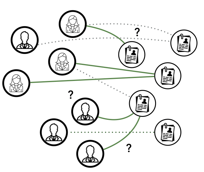
(a) Job recommendation

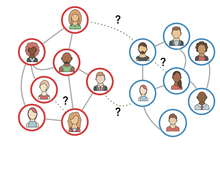
(b) Online polarization

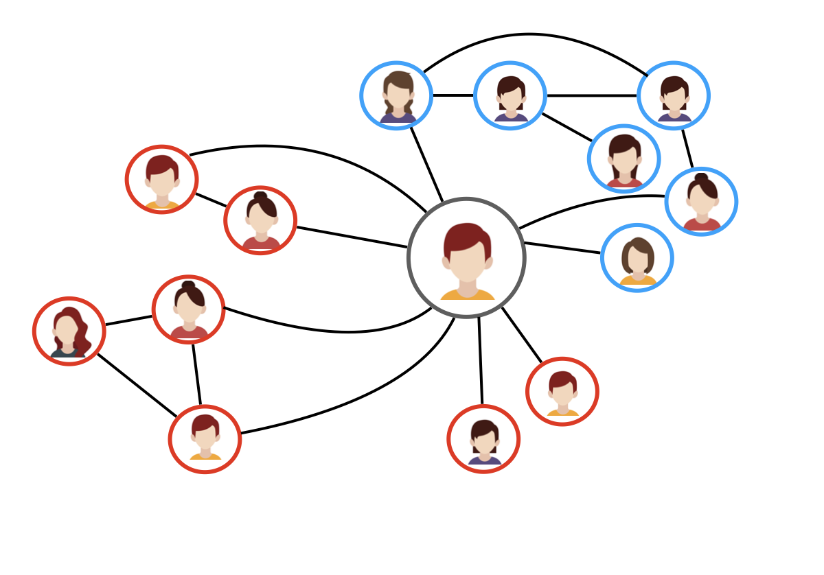
(c) Role of influencers

Figure 2. Examples of networks with two different potential bias: job-candidate matching (a) and a social media network with political echo chambers (b) and in the presence of an influencer node (c).

Social Networks

For our first example, we consider a social network of bloggers (see Figure 2(b)): in this context, a node represents a blogger, and two nodes are connected if the bloggers follow each other. We also assume that for each node we have access to multiple attributes, including the political inclination and the topics of interest. The political inclination can be considered as a protected attribute and such networks present a risk of partisan or political bias. Indeed, an edge prediction model might tend to promote only links between people having the same political ideology, since they are more likely to be connected in the network, which leads to the formation of online bubbles and online polarization. Another important source of bias is that social media networks tend to be centralized: a small number of nodes, so-called influencers, are at the center of the graphs, meaning that these nodes are connected to nearly all the other nodes (see Figure 2(c)). As a result, these influencers strongly impact the other nodes around and therefore the outcomes of any supervised or unsupervised models. The topic of fair influence maximization is left out from this survey, as to the best of our knowledge, only one article exists on the topic (Khajehnejad et al., 2021b).

Candidate-Job matching

(Kenthapadi et al., 2017) The job market and more precisely the job recruitment process is more and more reviewed and supervised using ML algorithms (Kenthapadi et al., 2017). As a result, one can ask if these automatic decisions are fair for all the applicants (see Figure 2(a)). Numerous studies demonstrate the presence of demographic biases in the different aspects of the job market, notably in the recruitment process (Oreopoulos, 2011; Bertrand and Mullainathan, 2003). In the context of machine learning, a recent paper studies the job platform XING, a professional social network and shows that it exhibits discrimination with respect to the gender, by ranking less qualified male candidates higher than more qualified female candidates (Lahoti et al., 2019). This problem of candidate/job matching can be represented by a bipartite graphs with two types of nodes : jobs and applicants. Both types come with attributes. For instance, for the applicants, we might have access to civil information, job title and previous salary. For the jobs, we can have access to a textual description and the proposed range for the salary. In this example, fair can have different meanings: on the one hand, we expect that a recommendation (link prediction between an applicant and a job) algorithm is independent of some sensitive attributes of the candidates, including, for instance, their gender or ethnic origin; we might also expect from a node regression model aiming to predict the salary of each candidate to also be independent from such attributes. This type of fairness is referred to as group fairness in the literature. On the other hand, we also expect the recommendation to remain fair from an individual point of view, i.e., two candidates with similar skills should obtain similar results. This type of fairness is usually referred to as individual fairness in the literature.

Next, we present the metrics proposed in the literature to evaluate bias at different steps of the edge prediction task.

3. Evaluation Metrics for Fairness

In this section, we present several metrics for group fairness assessment. These metrics are usually either derived from the domain of community detection in graphs, or from the domain of fair machine learning for tabular data.

3.1. Metrics for Fairness at the graph level

When considering the whole graph, the notion of homophily of the graph with respect to a particular attribute, that can be evaluated using the Assortative Mixing Coefficient (Newman, 2003), is of interest to assess the bias inherent to the graph structure itself. Mixing in social network analysis studies the tendency of nodes to connect with other nodes having similar attributes. In the context of dyadic fairness, the underlying idea is that the stronger the correlation between the community structure and the protected attribute (i.e. a coefficient with a value close to 1 or -1), the higher the risk of bias along the process. Figure 3 illustrates the idea. Thus, the graph $G1$ (a) has two communities, and these communities are almost completely defined by the protected attribute $A$. Going back to our online bubble example, where $A$ is the political inclination of the bloggers with $A=1$ for republicans and $A=0$ for democrats. In this example, it can be seen that republicans (and democrats) are more connected to each other rather than with bloggers with a different political opinion. As a direct consequence, the learned node embeddings will reflect this separation and a link prediction model which predicts links between nodes lying close in the embedding space will exclusively connect bloggers from the same political groups, resulting in an emphasis of this cleavage as illustrated in Figure 3 (b). On the other hand, when communities are independent from the protected attribute (Figure 3 (c)(d)), the graph does not present a risk of biased link prediction, and while the node embeddings preserve the graph structure, they cannot be used to retrieve $A$.

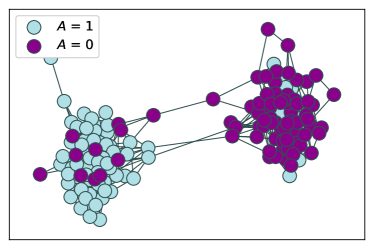
(a) G1, $r=0.51$

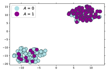
(b) G1 node embeddings

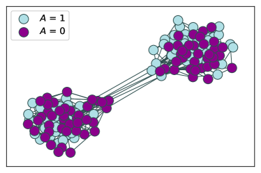
(c) G2, $r=0.04$

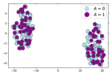
(d) G2 node embeddings

Figure 3. Illustration of the assortative mixing coefficient ($r$). Embeddings are computed with Node2Vec and a dimension of 8. The representation of node embeddings is done with TSNE.

Let us now formally define the assortative mixing coefficient. First, we consider the following quantity:

$$e_{ij}=\frac{card\{(i,j)\in\mathcal{E};A_{v_{i}}=i,A_{v_{j}}=j\}}{m},$$

where $m$ is the number of edges in the network. Note that when $i\neq j$, $e_{ij}$ corresponds to the fraction of edges in-between nodes having different values for their sensitive attributes, while when $i=j$, it corresponds to the fraction of edges in-between nodes belonging to the same protected group. The matrix defined by $e_{ij}$’s satisfies the property $\sum_{i,j}e_{ij}=1$, and we define $a_{i}=\sum_{j}e_{ij}$ and $b_{j}=\sum_{i}e_{ij}$ that describe the proportion of edges starting from and ending at each of the attribute values. Finally, the assortative mixing coefficient is defined by:

(1) $$r=\frac{\sum_{i}e_{ii}-\sum_{i}a_{i}b_{i}}{1-\sum_{i}a_{i}b_{i}}.$$

The coefficient $r$ takes values in $[-1,1]$, where $1$ corresponds to the perfectly assortative case, i.e. nodes with the same value for $A$ exclusively connect with each other; $-1$ corresponds to the dissortative case, i.e. nodes only connect with nodes having a different value for $A$. A fair graph will have a mixing coefficient of 0.

This coefficient $r$ can be simply computed on any graph to assess if the graph is biased or not (Laclau et al., 2020), or used to enforce fairness in the graph (Spinelli et al., 2021).

3.2. Metrics for Fairness at the representation level

Representation Bias (RB), originally proposed by (Bose and Hamilton, 2019), and then formalized by (Buyl and Bie, 2020), is used for evaluating the bias at the node embedding level. The underlying idea is to consider $A$ as the target variable. Given a node embedding vector as input, RB computes the weighted average over the one-versus-rest AUC scores obtained from the output $\mathbb{P}_{h}(a,z_{v})$ of a classifier $h$ trained to predict the protected attribute $A$. Defining by $V_{a}=\{v|A(v)=a\}$ the set of nodes taking the value $a$ for the protected attribute, the RB score is given by:

(2) $$RB=\sum_{a=0}^{l}\frac{1}{|V_{a}|}\text{AUC}(\{\mathbb{P}_{h}(a,z_{v})|\forall v\in V_{a}\}).$$

RB $\in[0,1]$ and is ideally close to $0.5$ meaning that the classifier learned from the node embeddings makes random prediction for the sensitive attribute. Compared to the other metrics, RB is not a dyadic-fairness criterion as it focuses on each node individually, and is therefore not sufficient to evaluate the fairness for edge prediction.

3.3. Dyadic Fairness Metrics

Now, we present metrics proposed to evaluate dyadic fairness, i.e., metrics that consider the bias at the relational level of the edges. Most of the criteria are properties of the joint distribution of the sensitive attribute $A$, the target variable $y$, and the learned edge predictor $h$.

Disparate impact (DI)

Originally proposed by (Barocas and Selbst, 2016) for tabular data, and then extended to graph in (Laclau et al., 2020) is considered as the discrimination that occurs unintentionally and is computed for the positive outcome for the privileged and underprivileged groups. It is calculated as the ratio between the underprivileged group with the positive outcome and the privileged group with the positive outcome. In our context, we can formulate DI as follows.

Definition 3.1.

Given a graph $\mathcal{G}=(\mathcal{V},\mathcal{E})$ and a function $h:\mathbb{V}\times\mathbb{V}\rightarrow\{0,1\}$, the disparate impact is defined as

$$\text{DI}(h,\mathbb{V},A)=\frac{\mathbb{P}(h(v_{i},v_{j})=1|A_{v_{i}}\oplus A_{v_{j}}=1)}{\mathbb{P}(h(v_{i},v_{j})=1|A_{v_{i}}\oplus A_{v_{j}}=0)},$$

where $\oplus$ stands for the XOR operator, and $A_{v_{i}}\oplus A_{v_{j}}=1$ (resp. $A_{v_{i}}\oplus A_{v_{j}}=0$) denotes the fact that nodes $v_{i}$ and $v_{j}$ belong to the same group (resp. different groups). A DI closes to $1$ indicated a fair situation.

One may note that the difference from the definition considered in (node) classification task with $\mathbb{V}\subset\mathbb{R}^{d},\ h:\mathbb{V}\rightarrow\{0,1\}$, comes from the fact that we deal with tuples and implicitly attribute a sensitive variable defined by $A_{v_{i}}\oplus A_{v_{j}}$ to each pair of nodes or, equivalently, to an edge. Let us consider the job market problem, one can consider a fair node classification task, where the goal is to predict the job category of a given candidate, independently from the gender of the candidate. In that case, the DI corresponds to the ratio of $P(h(v_{i})=nurse|A=female)$ and $P(h(v_{i})=nurse|A=male)$ for instance, and a fair situation corresponds to the equality of these two quantities, i.e., DI=1. Now, let us consider the slightly different but common task for online professional networks: candidate-candidate matching, i.e., recommending to a given user whom to connect with. In that context, the input consists of two users, hence our objective is to ensure an equal probability to connect two users independently from the fact that they are both men or women (denoted by $A_{v_{i}}\oplus A_{v_{j}}=0$). In both cases, the value of $DI$ has the same interpretation.

Another formulation of the DI known as statistical parity or demographic parity has also been used and explored in the context of graphs. ((Rahman et al., 2019)). Formally, we can define statistical parity as follows.

Definition 3.2.

Given a graph $\mathcal{G}=(\mathcal{V},\mathcal{E})$ and a function $h:\mathbb{V}\times\mathbb{V}\rightarrow\{0,1\}$, statistical parity for an edge predictor $h$ on $A$ with respect to $\mathbb{V}$ is given by:

$$\mathbb{P}(h(v_{i},v_{j})=1|A_{v_{i}}\neq A_{v_{j}})=\mathbb{P}(h(v_{i},v_{j})=1|A_{v_{i}}=A_{v_{j}})$$

or equivalently

$$\mathbb{P}(h(v_{i},v_{j})=1|A_{v_{i}}\oplus A_{v_{j}}=1)=\mathbb{P}(h(v_{i},v_{j})=1|A_{v_{i}}\oplus A_{v_{j}}=0),$$

where $\oplus$ stands for XOR operation as stated in the definition of DI.

In practice, the goal is to reduce the gap between these two probabilities. While these metrics are popular and easy to control, they might not be restrictive enough for certain applications as they solely focus on true positive outcomes.

Equal Opportunity (EO)(Hardt et al., 2016b)

This metric is different from the aforementioned metrics as it acknowledges that in many scenarios, the sensitive characteristic may be correlated with the target variable.

Definition 3.3.

Equal Opportunity (EO), in the context of edge prediction can be formulated as follows.

$$P(h(v_{i},v_{j})=1|y_{uv}=1,A_{u}=A_{v})=P(h(v_{i},v_{j})=1|y_{uv}=1,A_{u}\neq A_{v}).$$

In the literature, this measure is usually expressed as a difference:

(3) $$\Delta EO=|P(h(v_{i},v_{j})=1|y_{uv}=1,A_{u}=A_{v})-P(\hat{h}(v_{i},v_{j})=1|y_{uv}=1,A_{u}\neq A_{v})|.$$

Note that $\Delta EO\in[0,1]$, where $0$ represents a fair situation.

Going back to our candidate-candidate matching task, statistical parity focuses on having the positive outcome independent of the protected class, e.g, $P(h(v_{i},v_{j})=follow|(A_{i}=female,A_{j}=male))=P(h(v_{i},v_{j})=follow|(A_{i}=male,A_{j}=male))$. Equal Opportunity requires the outcome to be independent of the protected class $A$, conditionally on the actual label $y$. A direct consequence of this additional assumption is to reduce the risk of blindly predicting links between users to fill in the gap between two protected groups.

Acceptance Rate Parity (Rahman et al., 2019)

Finally, this metric is a ranking-based measure introduced to evaluate fair edge prediction.

Definition 3.4.

The acceptance rate accounts for the relative frequency for which a link between two nodes with different attributes $A(v_{i})=a$ and $A(v_{j})=b$ appears in the overall top-k highest prediction scores. For a given node $v_{i}$ the list of its link recommendations is denoted by $\rho_{v_{i}}$, and $v_{j}\in\rho_{v_{i}}$ indicated that a link has been predicted between $v_{i}$ and $v_{j}$.

(4) $$\alpha_{x,y}=\frac{1}{N_{x,y}}|\{(v_{i},v_{j})|v_{j}\in\rho(v_{i}),v_{i}\in V_{x},v_{j}\in V_{y}\}|$$

where $N_{a,b}$ represents all possible combinations between the nodes having attribute values $a$ and $b$ and can be given as,

$$N_{a,b}=|\{(v_{i},v_{j})|v_{i}\in V_{a},v_{j}\in V_{b}\}|.$$

A high value of the ARP indicates a fair situation. Note that this metric depends on the length of the considered list of predictions for a given node.

Let us illustrate this metric with our previous example. We first consider, a given user $i$, with protected attribute $A_{i}=female$, then look at the attributes of the top-5 candidates recommended to this particular user: $(A_{1},A_{2},A_{3},A_{5})=female$, $A_{4}=male$. The ARP counts the relative frequency of males in the top-5, here $\frac{1}{5}$, meaning that the model decision is unfair. While ARP is intuitive and easy to interpret, it presents the same weakness as the DI or statistical parity, as it does not account for the relevance of the prediction along with the protected attribute. Hence, models that are simply moving up male in the top-5 list regardless of their relevance for that particular user will be considered fair, while they negatively impact individual fairness notions.

As stated in the introduction, fairness can be imposed at different stages of the machine learning process. The next sections are dedicated to a presentation of methods proposed to address fairness in the context of graphs. Table 1 sum-up existing contributions described hereafter and provides links to the available implementations.

4. Repairing Bias at the Origin

Table 1. Summary of all methods reviewed in this paper and a link to the available implementations. Note that a * means that the implementation is not the official one (i.e. not proposed by one of the authors of the paper). NA stands for Not Available. Row colors groups methods falling in the same category.

Method	Reference	Code	Pre-processing	In training	Post-processing	Keywords
FairOT	(Laclau et al., 2020)	Github	✓			Optimal Transport, Laplacian regularization
FairDrop	(Spinelli et al., 2021)	Github	✓			Edge Drop, Homophily
UGE	(Wang et al., 2022)	NA	✓			Structural generative graph model
FairWalk	(Rahman et al., 2019)	Github∗		✓		Random walk
CrossWalk	(Khajehnejad et al., 2021a)	Github		✓		Random walk
DeBayes	(Buyl and Bie, 2020)	Github		✓		Conditional Network Embeddings, Bayeisan prior
FIPR	(Buyl and Bie, 2021)	Github		✓		I-Projection regularizer
CFC	(Bose and Hamilton, 2019)	Github			✓	Adversarial Learning, Compositional filtering
FLIP	(Masrour et al., 2020)	Github			✓	Adversarial Learning, Modularity
DKGE	(Fisher et al., 2020)	NA			✓	Adversarial, Knowledge graphs
FairGNN	(Dai and Wang, 2021)	Github			✓	GNNs, Adversarial Learning
FairAdj	(Li et al., 2021)	Github		✓		Graph Neural Networks
MONET	(Palowitch and Perozzi, 2020)	Github		✓		GNNs, metadata
NIFTY	(Agarwal et al., 2021)	Github		✓		GNNs, augmented views, stability
InFoRM	(Kang et al., 2020)	Github	✓	✓	✓

The first family of models aims at removing bias from the graph structure itself. As a result, these methods can then be combined with any node embedding techniques, which makes them quite flexible. However, one should bear in mind that in this case, nothing prevents the node embedding models or even the classifier used afterward from retrieving signal about the protected attribute. Among these methods, we can present FairOT (Laclau et al., 2020) and FairDrop (Spinelli et al., 2021).

In FairOT, the authors propose an embedding-agnostic procedure to repair the original graph using optimal transport technique with a focus on the fair link prediction task. To this end, they propose to cast the problem of debiasing the graph as a problem of alignment between node distributions of nodes belonging to different protected groups, where the latter are taken to be the rows of the normalized adjacency matrix. Their proposition is derived from a theoretical analysis of the disparate impact. In addition, their approach is the first one that allows to explicitly control the trade-off between individual and group fairness through a Laplacian regularization term added to the optimal transport objective. The model is evaluated on both synthetic graphs and real-world benchmark for the task of edge prediction.

FairDrop is also a pre-processing technique that modifies the adjacency matrix during a training step to compensate the homophiliy due to the sensitive attribute. This approach is based on a biased edge dropout which consists at each step of the training to remove edges between the linked nodes according to a randomized response mechanism that cuts more links between nodes having the same sensitive attribute value. The authors evaluate FairDrop on link prediction, both through a random walk model for building node embeddings and in a graph convolutional network able to solve the task in an end-to-end fashion. Compared with some in-processing methods, the experimental results obtained on traditional benchmark show that FairDrop decreases the RB with a negligible drop in accuracy.

Finally, the most recent approach that falls into this category is the Unbiased Graph Embedding UGE (Wang et al., 2022) framework. This approach relies on similar principles that the aforementioned ones, and the authors propose to generate a new bias-free graph by reducing the dependence between the structure of the observed graph and the effect of the sensitive attribute. They evaluate the performance of their approach using well-known graph neural network architectures.

5. Learning fair node embedding

Most of the research works dedicated to fair link prediction, focus on achieving fair node representation learning, as one can demonstrate that fair node embedding results, when evaluated by demographic parity, in fair link prediction (Li et al., 2021).

5.1. Methods based on existing node embedding models

To the best of our knowledge, the first model proposed to address the problem of fairness for graphs is Fairwalk(Rahman et al., 2019): a fair extension of Node2vec. Fairwalk, relies on a modification of the random walks to induce more fairness. This method modifies the transition probability of Node2vec for the generation of unbiased traces and can be detailed in the following two steps.

1. First, a corpus of traces is generated by performing random walks. Formally, denoting by $c_{i}$ the $i$-th node in a given walk, the next node is selected among all neighbors of $c_{i}$, i.e.,

   $$\mathbb{P}(c_{i+1}=v|c_{i}=u)=\left\{\begin{array}[]{ll}\frac{1/k}{|A_{N_{u}}^{k}|}&\mbox{if }A_{v}^{k}=1\mbox{ and }\{u,v\}\in\mathcal{E}\\ 0&\mbox{otherwise,}\end{array}\right.$$

   where $k\in\{1,\cdots,K\}$ denotes the modality of the sensitive attribute $A$, $A_{N_{u}}^{k}$ is the number of nodes in the neighborhood of $u$ belonging to the group $k$ and $A_{v}^{k}=1$ indicates that node $v$ belongs to the $k$-th group of the sensitive attribute. As a result, each generated random walk has a higher probability to contain nodes of different groups.

2. Then, Fairwalk uses the generated corpus to learn the embedding vectors through a SkipGram architecture that maximizes the log-probability of observing a network neighborhood for a node conditioned on its feature representation:

   $$\underset{Z}{\mathrm{argmax}}\ \prod_{u\in\mathcal{V}}\prod_{v\in N_{u}}\mathbb{P}(v|Z(u)).$$

Fairwalk works well on graphs in which the neighbouring nodes have different sensitive attributes, for example the graph $G_{2}$ presented in Figure 3(c). However, one can expect this model to fail in extreme cases such as the graph $G_{1}$ presented in Figure 3(a), as during the random walks, only the nodes belonging to the same group will be discovered in the direct neighborhood of a given node.

In the same spirit, CrossWalk (Khajehnejad et al., 2021a) is based on a re-weighting procedure for building the random walks and can therefore be used with any random walk based algorithms including DeepWalk (Perozzi et al., 2014) and Node2vec (Grover and Leskovec, 2016), to name a few. CrossWalk aims to address the shortcomings of Fairwalk by assigning more weights to both edges that connect nodes on the boundary of the protected groups, and edges connecting nodes from different groups. It has been evaluated in various graph-related tasks such as link prediction, node classification and influence maximization. and iy obtained superior results than Fairwalk, resulting from the group peripheries exploration.

Different from the aforementioned techniques, Debayes (Buyl and Bie, 2020) is a Bayesian approach based on the Conditional Node Embeddings (CNE) (Kang et al., 2019) method, where the sensitive information is modeled in the prior distribution. Given a graph $G=(V,E,A)$, CNE finds an embedding Z by maximizing $P(G|\textbf{Z})=\frac{P(\textbf{Z}|G)P(G)}{P(\textbf{Z})}$. The prior knowledge about the node degree is modeled by the prior distribution $P(G)$, expressed by the following constraint:

(5) $$\sum_{v\in V}P((v,v^{\prime})\in E)=\sum_{v\in V}\mathds{1}\left((v,v^{\prime})\in\mathcal{E}\right).$$

Debayes extends CNE, with a prior to model the sensitive attribute by replacing the constraint (5) with:

$$\sum_{v\in V_{s}}P((v,v^{\prime})\in E~{}|~{}A(v)=k)=\sum_{v\in V_{k}}\mathds{1}\Big{(}(v,v^{\prime})\in\mathcal{E}\Big{)},$$

where $V_{k}=\{v|A(v)=k\}$. With this prior, debiased embeddings, containing minimal information about sensitive attribute, are obtained during the training step.

Finally Fairness Regularizer (FIPR) (Buyl and Bie, 2021) generalizes the idea of DeBayes by proposing a regularization term to encourage fair link prediction that can be applied with any probabilistic network models. This regularizer is defined by the KL-divergence between the probabilistic node embedding model and its I-projection. One of the strengths of FIPR is its ability to be flexible both with respect to the node embedding approach but also with respect to the fairness metric.

5.2. Adversarial Approaches

A popular approach to achieve fairness in machine learning for tabular data is to leverage the principles of adversarial models (Madras et al., 2018; Grari et al., 2020; Adel et al., 2019).

For fair graph mining, one can mention Compositional Fairness Constraints (CFC) (Bose and Hamilton, 2019) that aims to generate node embeddings that are invariant of the sensitive attributes. To accomplish this, the authors train a set of filters (for the sensitive attributes) such that the adversarial discriminators are unable to classify the sensitive attribute from the filtered embedding. Hence, the goal is to minimize the mutual information between the filtered embedding and the protected attributes. These filters are defined for potentially multiple sensitive attribute $m$ as $f_{m}:\mathcal{R}^{d}\rightarrow\mathcal{R}^{d}$ and are trained to remove the sensitive information about the $m^{th}$ attribute (see an illustration in Figure 4). Note that this approach is the only one that can consider several protected attributes simultaneously. Then, the filtered embedding becomes the input to the adversarial discriminators which try to predict the sensitive attribute of the nodes. As a result, this approach particularly focuses on reducing the representation bias (RB) presented in Section 3. However, by processing nodes individually, CFC is not considering the problem of dyadic fairness.

Figure 4. CFC: the graph $G$ comprises of nodes with sensitive attributes such as age, gender, etc. The node embeddings ${z}_{i}\in\mathbb{R}^{d}$ for $G$ are informative of these sensitive attributes. Compositional Fairness Embeddings $\tilde{z}_{i}\in\mathbb{R}^{d}$ are generated after filtering out the sensitive information with the help of Discriminators.

While CFC considers the representation bias, Fairness-Aware Link Prediction (FLIP) (Masrour et al., 2020) proposes an adversarial architecture focusing on controlling the impact of graph level metrics for fairness. More precisely, the authors address fairness through the lens of modularity, which in their case is similar to homophily. To proceed, they post-process the prediction output of their model so as to reduce the modularity of the predicted network: this model encourages predictions of more inter-group links than in the original network. The detailed architecture and working of the model are shown in Figure 5. They evaluate their model on rather small graphs for the task of link prediction and compare it with post-processing methods focusing on the equalized odds metric.

Figure 5. FLIP Architecture: The generator takes an attributed network as input and learns a representation for each node. FLIP uses DeepWalk (Perozzi et al., 2014) as the generator, other representation learning frameworks can also be used. The Discriminator takes as input the representation for each pair of nodes and tries to predict if it belongs to intra-group or inter-group. The link prediction component takes as input the learned node representations and tries to predict if there is a link.

FairGNN (Dai and Wang, 2021) focuses on the problem of learning fair Graph Neural Network (GNN) representations in the presence of partial sensitive attribute information. The authors consider the problem of node classification and propose to mitigate bias by using adversarial debiasing on the final layer of the GNN i.e., the learned node representations. The main drawback of this model is its limitation to the node classification task. We will give more details in the next Section dedicated to neural network-based models.

Finally, Debiasing Knowledge Graph Embeddings (DKGE)(Fisher et al., 2020) is an approach that focuses on learning fair embeddings for knowledge graphs such that these embeddings are neutral to the sensitive attribute by using an adversarial loss. The objective is to balance the outcome with respect to each of the protected groups. To this end, a penalization term is added; it is defined by the KL-divergence between the distribution of the outcome and a balanced distribution. This approach is evaluated with the accuracy of the embeddings on the triple prediction problem, a traditional task for knowledge graphs. A comparison with CFC shows superior performance. In addition, it demonstrates that CFC struggles to maintain a good accuracy while reducing the bias but also suffers from leaking of information when used for multiple sensitive attributes.

5.3. Graph Neural Networks based models

Graph Neural Networks (GNN) models have recently established themselves as state-of-the-art for the graph-related downstream tasks. These models usually consider two types of input to learn a good representation: the graph structure (usually in the form of an edge list or the adjacency matrix), and a matrix of node attributes. However, GNNs, by design, model the homophily principle: for given node attributes, similar nodes may be more likely to connect to each other than dissimilar ones. As a result, these models are also more prone to produce biased prediction as one can show that homophily is strongly related to bias (see Section 3). Therefore, it comes with no surprise that most of the recent approaches are dedicated to constraining GNNs to produce more fair outcomes.

(a) MONET

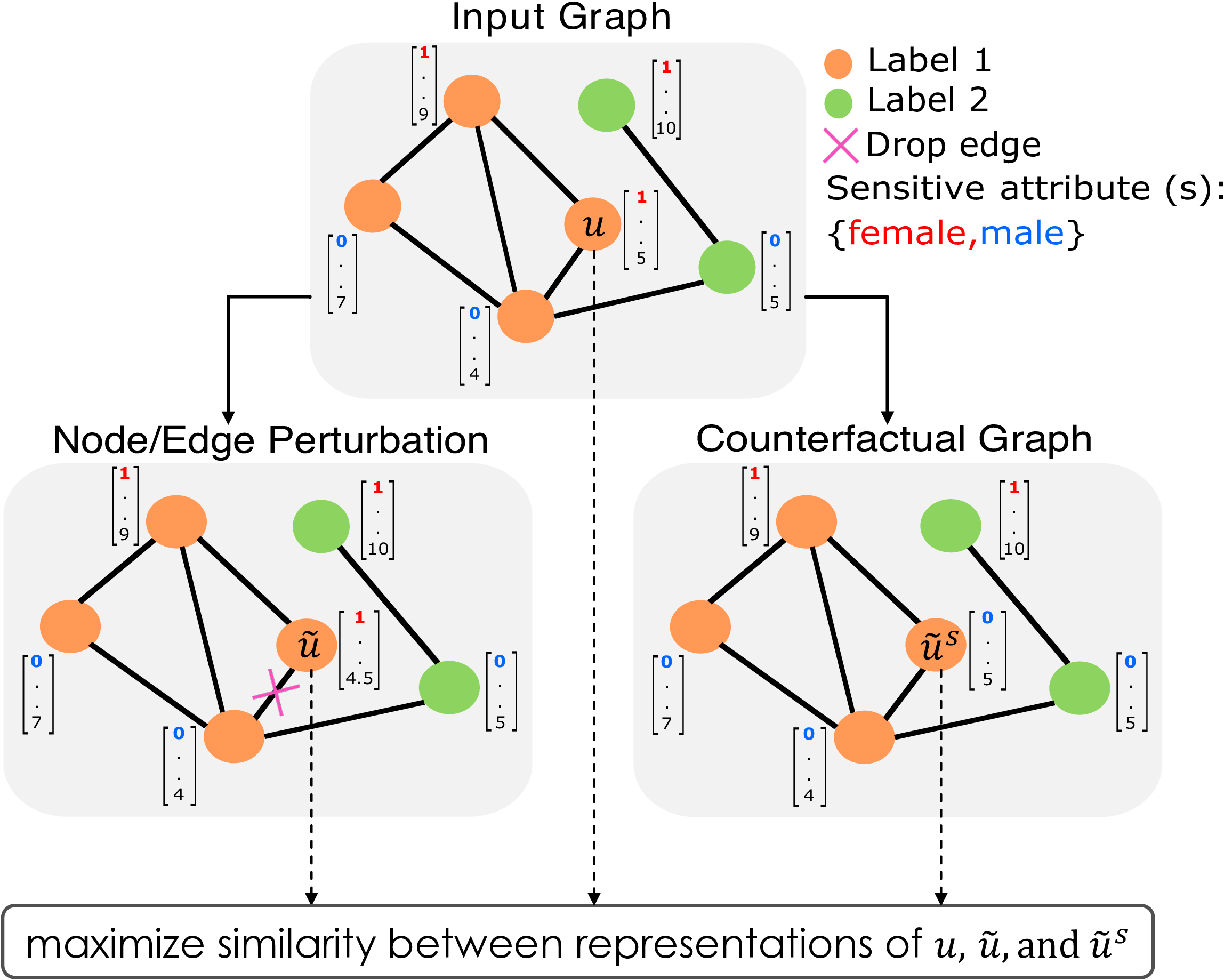
(b) NIFTY

Figure 6. Illustration of two GNN based models for graph fairness: (a) MONET(Palowitch and Perozzi, 2020) which imposes independence (through orthogonality constraints) between the embedding spaces of features and topology; and (b) NIFTY (Agarwal et al., 2021) that generates perturbated and counterfactual graphs to ensure stable node representation. Images are taken from original papers.

The first proposition in that direction is the Metadata-Orthogonal Node Embedding Training (MONET) model (Palowitch and Perozzi, 2020), which performs debiasing of node embeddings at training time with a neural network component coined with the term MONET unit. The model learns jointly a graph topology embedding matrix and a graph metadata embedding matrix while enforcing linear independence between the two embedding spaces through Singular Value Decomposition (SVD). The prime limitation of this approach relies on the fact that it only performs a linear debiasing and as a result, the embeddings learned with MONET are only fair with respect to linear models for the edge prediction task. Thus, non-linear models (e.g., support vector machines with non-linear kernels) are able to retrieve part of the bias directly from the embeddings. The performances of the model are evaluated, in terms of representation bias, by considering node classification on the sensitive attributes and on shilling attacks where several users act together to artificially increase the likelihood that a particular influenced item will be recommended for a particular target item. An illustration of the proposal is given in Figure 6(a).

The work of (Li et al., 2021) relies on the same principle as the pre-processing models and Crosswalk but leverages the power of GNNs. The authors propose to modify the adjacency matrix of the graph while training node embeddings with a GNN. They notably demonstrate that fair vertex representations is a sufficient condition to achieve demographic parity (group fairness) in link prediction. To proceed they propose a reweighing schema of the edges (intra and inter) that guarantees a reduction of the representation discrepancy between two sensitive groups. They implement their proposal within the framework of variational graph auto-encoders (Kipf and Welling, 2017) and show that it can outperform adversarial training with various fairness-accuracy trade-off.

In (Agarwal et al., 2021), the authors propose to address two weaknesses of GNNs : stability and fairness, where the latter is defined as counterfactual fairness. We remind that counterfactual fairness accounts for robustness w.r.t modifying the sensitive attribute while stability accounts for robustness w.r.t perturbing the node attributes and/or link information. To proceed, they propose a new versatile framework, named NIFTY (uNIfying Fairness and stabiliTY), that has the ability to encompass several GNNs architectures. NIFTY proposes to modify both the objective loss and the architecture of the GNNs to tackle the problems of stability and fairness. It relies notably on the generation of augmented views of the original graph with counterfactual nodes and perturbated edges and the Lipschitz constant to develop layer-wise weight normalization. Overall, it demonstrates superior performance by a large margin than FairGNN (Dai and Wang, 2021) and proposed NIFTY versions of Graph Convolutional Network (Kipf and Welling, 2017) and GraphSage (Hamilton et al., 2017). An illustration of the general idea of NIFTY is provided in Figure 6(b).

The work presented in (Ma et al., 2021) is not an algorithmic contribution but a theoretical analysis that allows to get insights on when to expect accuracy disparity across subgroups of nodes. In this work, the authors propose a novel PAC-Bayesian analysis on the generalization ability of GNNs with non-IID assumptions for graphs and then, they use this result to acknowledge the unfairness of GNN outcomes. They propose an empirical analysis to verify the existence of this accuracy disparity for multiple GNN models, including GCN (Kipf and Welling, 2017), GAT (Velickovic et al., 2018), SGC (Wu et al., 2019a), and APPNP (Klicpera et al., 2019).

Finally, we conclude this Section with INFORM (Kang et al., 2020), as it differs from all previously aforementioned models. In this work, the authors first propose to study the notion of individual fairness in the context of graph mining and derive several metrics for both individual as well as group fairness. They further proposed three algorithmic contributions to optimize these metrics: 1) a pre-processing step to debias the input graph; 2) an in-processing step to debias the mining model; and 3) a post-processing step to debias the model outcome. They instantiated their framework with PageRank (Page et al., 1999) and LINE (Tang et al., 2015) for link prediction, and with a spectral clustering model for community detection.

6. Benchmark Graphs

In this section, we start by introducing a set of synthetic graphs that can be used to evaluate fairness and, propose an additional setting for multiple sensitive attributes. Then, we present an overview of existing benchmark graphs that can be used to work on the problem of fair edge prediction. Codes to reproduce the synthetic graphs as well as a direct link to download the benchmark graphs can be found at: https://github.com/manvic14/Survey_Fairness_Graphs.

6.1. Synthetic Graphs

Synthetic graphs can allow to better understand the behaviour of a model in a controlled experimental environment and to identify possible weaknesses. We describe hereafter the synthetic scenarios and the generative process associated with it, introduced in (Laclau et al., 2020).

The authors propose to generate five synthetic graphs (G1–G5) composed of 150 nodes each (note that this number can be easily increased) based on the stochastic block model with different block parameters. This latter is done using the networkx library . Following a similar process, we propose to add a sixth scenario, referred to as (G6) in the following. We believe that this scenario could be particularly helpful to the research community, as very few models can handle it. For the sake of reproducibility, we provide some of the parameters used to generate the graphs in Table 2. In addition, we report the average values of the assortativity mixing coefficient obtained over 10 trials. Note that this criterion, as explained in Section 3, amounts to measuring the potential bias that one can expect when dealing with such structure. Each node is associated with one or multiple sensitive attributes. For the first four graphs, this sensitive attribute is binary, for G5 $S$ is a multiclass attribute taking three modalities (K=3). Using the same protocol, we propose G6, which corresponds to a graph with two binary protected attributes.

Hereafter, we describe in more depth each of the graph structure:

• G1 corresponds to a graph with two communities and a strong dependency between the community structure and the sensitive attribute $S$;

• G2 has the same community structure as G1, but with $S$ being independent of the structure;

• G3 corresponds to a graph with two imbalanced communities dependent on $S$ and a stronger intra-connection in the smaller community;

• G4 is a graph with three communities, two of them being dependent on $S$, and the third one being independent;

• G5 is a multiclass version of G4 with three communities, each of them being dependent on one of the modalities of the protected attribute;

• G6 corresponds to the multiple attributes case, that only very few approaches can handle. The two protected attributes are distributed along with the three communities. The first attribute, denoted by $A$ is correlated with the community structure, while the second one, $A^{\prime}$ is randomly distributed.

Figure 7 illustrates each scenario with a graph generated according to the parameters of this latter.

Table 2. Parameters used for graph generation. Cluster implies that the value of $S$ is almost equal to the community identifier, while random implies that $S$ is randomly generated and is independent from the community structure of the graph. $\bar{r}$ is the average of the assortativity coefficients obtained for 10 simulations with similar parameters.

Graphs	$S$	$|S|$	Size	#S	$\bar{r}$
G1	cluster	2	$\begin{pmatrix}75&75\end{pmatrix}$	1	$.768\pm{.055}$
G2	random	2	$\begin{pmatrix}75&75\end{pmatrix}$	1	$.001\pm{.035}$
G3	cluster	2	$\begin{pmatrix}125&25\end{pmatrix}$	1	$.711\pm{.082}$
G4	random & cluster	2	$\begin{pmatrix}50&50&50\end{pmatrix}$	1	$.576\pm{.037}$
G5	cluster	3	$\begin{pmatrix}50&50&50\end{pmatrix}$	1	$.732\pm{.041}$
G6	cluster	2	$\begin{pmatrix}50&50&50\end{pmatrix}$	2	-

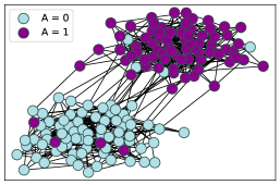
(a) G1

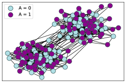
(b) G2

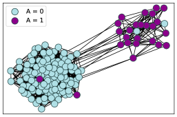
(c) G3

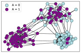
(d) G4

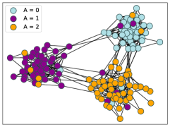
(e) G5

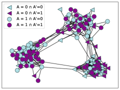
(f) G6

Figure 7. Synthetic graphs proposed to address fairness in graphs. $\textsc{G1}-\textsc{G5}$ were initially proposed by (Laclau et al., 2020). G6 is a new scenario.

6.2. Real-world Graphs

Hereafter, we propose a list of the real-world graphs commonly used in papers dedicated to fairness for graphs. Table 3 provides both statistics on the graphs and information related to the protected attribute(s). This list along with a link to download the benchmarks is available on the repository of the survey.

6.2.1. Benchmarks with binary sensitive attribute

Polblogs(Adamic and Glance, 2005) is a political blogosphere network of the US for February 2005. In this graph, the nodes represent blogs and vertices represent the hyperlinks between the two blogs. In this context, the political leaning associated with the node, which is either liberal (0) or conservative (1) is the sensitive attribute.

Facebook-E  (McAuley and Leskovec, 2012) and Google+  are two collections of ego networks of the Facebook app and Google+ users, respectively. For Facebook-E, the combined version consists of the aggregated networks of Facebook friend lists for ten individuals. Google+  comprises ego-networks of 133 users whose information was publicly accessible at the time of the crawl and included only the users who had shared at least two circles. In both cases, the sensitive attribute is the gender information corresponding to each node. A particularity of Facebook-E  is that it structure is not particularly dependent on the sensitive attribute, making this latter a good candidate for a sanity check (i.e., one should expect stable results with or without group fairness constraints).

NBA  (Dai and Wang, 2021) contains performance statistics of players in the 2016-2017 season along with information such as nationality, age and salary for 400 NBA basketball players. The graph connecting these NBA players is obtained using their relationships on Twitter. All the information can be considered a potentially sensitive attributes: the nationality of the players which is binary (American players vs. overseas players) but also their age and salary.

6.2.2. Benchmarks with categorical sensitive attribute

LastFM  Asia Social Network (Rozemberczki and Sarkar, 2020) is a network collected from the LastFM  public API in March 2020. In this network, the nodes represent the LastFM  users and the edges represent the mutual follower relationships between the users. The sensitive attribute is the country of the user and takes 18 modalities. One should note that a particularity of the graph is that the distribution of the modalities of the country is very imbalanced.

Facebook-P  (Rozemberczki et al., 2019) is a page-page graph of verified facebook sites. The nodes correspond to the official Facebook pages and there exists a link between the nodes if there exist mutual likes between the sites. The page-type is treated as the sensitive attribute. The page-type can take 4 values: company, government, politician and tvshow.

Pokec  (Takac and Zabovsky, 2012) is a very popular widely used online social network in Slovakia (similar to Facebook and Twitter). Nowadays, Pokec  counts approximately 1.6 million users. This dataset comprises anonymized data of the whole network. Since the dataset is large, in (Dai and Wang, 2021), the authors sample two datasets (based on the provinces the users belong to) from the original Pokec  dataset namely Pokec-z and Pokec -n. Several attributes can be used as sensitive including the region, gender and age of users.

DBLP  is a co-authorship network constructed from the computer science bibliography database. The version proposed by (Buyl and Bie, 2020) is considered where the publications in specific conferences are taken into account. The continent is the sensitive attribute and it is extracted from the author’s country of affiliation. The continents Africa and Antarctica are not considered due to a strong under-representation in the data.

Table 3. Descriptive Statistics of Benchmark Graphs used in the context of Fair Edge Prediction. Attributes are categorized as Cat. (categorical) or Cont. (continuous). A “–” indicates that the property cannot be computed (for instance the $r$ mixing coefficient for continuous attributes).

	Networks
Properties	PolBlogs	Facebook-E	Pokec-z	Pokec-n	LastFM	Facebook-P
# of nodes	$1,490$	$4,039$	$67,797$	$66,569$	$7,624$	$22,470$
# of edges	$19,090$	$88,234$	$617,958$	$517,047$	$27,806$	$171,002$
Type of attributes	Cat.	Cat.	Cat.	Cat.	Cat.	Cat.
Attribute Name	Party	Gender	Region	Region	Country	Page-type
# of inter-group edges	$1,575$	$41,875$	$30,519$	$24,293$	$3,507$	$19,590$
# of intra-group edges	$15,203$	$46,359$	$587,439$	$492,754$	$24,299$	$151,412$
Mixing Coefficient $r$	$.81$	$.09$	$.87$	$.89$	$.86$	$.82$
Properties	MovieLens-1M	MovieLens-100K	DBLP	Reddit	Google+	NBA
# of nodes	#users $6,040$,#movies $3,900$	$\#$users $943$,$\#$movies $1,682$	$3,980$	$385,735$	$4,938$	$400$
# of edges	$1,000,209$	$100,000$	$6,965$	$366,797$	$547,923$	$10,621$
Type of attributes	Cat.,Cont.	Cat.,Cont.	Cat.	Cat.	Cat.	Cat., Cont.
Attribute Name	(Gender, Occupation, Age)	(Gender, Occupation, Age)	Continent	Subreddits	Gender	(Salary,Country,Age)
# of inter-group edges	$-$	$-$	$669$	$-$	$-$	$(2,935;4,166;-)$
# of intra-group edges	$-$	$-$	$5,887$	$-$	$-$	$(7,686;6,455;-)$
Mixing Coefficient $r$	$-$	$-$	$.84$	$-$	$-$	$(.015,.218,-)$

6.2.3. Bipartite graphs benchmarks

MovieLens  is a collection of bipartite graphs consisting of user-movie ratings, on a scale of one to five. Nodes can therefore be of two types (users or movies) and an edge indicates that a user has rated a particular movie. For each user, the data set provides meta-information including gender, occupation and age. The user features are considered as sensitive attributes. Two versions of this dataset are traditionally used to evaluate graph fairness contributions, namely MovieLens-100K and MovieLens-1M.

Reddit  (Bose and Hamilton, 2019) is a dataset from the popular discussion website where the registered members submit content. These posts are organized by subject covering various topics and called ”communities” or ”subreddits”. The dataset is described in (Bose and Hamilton, 2019). The authors propose considering the comments from the month of November 2017, and define an edge between a user and a community if the user commented at least once on that community during this period. The low-degree nodes were removed to obtain the final graph with 366K users, 18K communities, and 7M edges. Reddit does not have public user attributes and the obtained graph is bipartite, so the attributes needed to be assigned to the users as well as the communities. Certain subreddits / node communities were treated as sensitive nodes and the sensitive attribute of the user was based on whether or not the user is connected to the sensitive community.

7. Open Challenges

While fairness has gained significant attention in graph-based machine learning and mining over the past three years, much remains to be done to mitigate the problem of biased decisions for this particular type of data. In this section, we present some of the remaining challenges in fair graph mining, and an overview of opportunities for future research. Table 4 summarizes some of the main properties of the state-of-the-art models aforementioned to highlight some pitfalls or gaps of current existing contributions.

Table 4. Outline of related work in terms of fulfilled (✓) and missing properties (✗) of the algorithms. Cat. stands for categorical while Cont. stands for continuous. $k$ denotes the number of modalities that $A$ can take and $|A|$ denotes the number of sensitive attributes. For the fairness criteria we distinguished between individual (Ind.), group (Group) and counterfactual (Count.) fairness and Representation Bias (RB). Note that this property indicates which criteria is the model based on to achieve fairness. Row color groups for methods falling in the same category. For INFORM the notion of sensitive attribute does not apply as it only considers individual fairness criteria.

	Type of Graphs			Attribute’s properties					Fairness Criteria
Method	Directed	Bipartite		Cat.	$k>2$	Cont.	$|A|>1$		Ind.	Group	Count.	RB
FairOT	✓	✗		✓	✓	✗	✗		✓	✓	✗	✗
FairDrop	✗	✗		✓	✓	✗	✗		✗	✓	✗	✗
UGE	✗	✗		✓	✓	✗	✗		✗	✗	✗	✓
Fairwalk	✗	✗		✓	✗	✗	✗		✗	✓	✗	✗
Crosswalk	✗	✗		✓	✓	✗	✗		✗	✓	✗	✗
DeBayes	✗	✓		✓	✓	✗	✗		✗	✓	✗	✗
FIPR	✓	✓		✓	✓	✗	✗		✗	✓	✗	✗
CFC	✓	✓		✓	✓	✗	✓		✗	✗	✗	✓
FLIP	✗	✗		✓	✗	✗	✗		✗	✓	✗	✓
DKGE	✗	✗		✓	✓	✗	✓		✗	✗	✗	✓
FairAdj	✗	✗		✓	✗	✗	✗		✗	✓	✗	✗
FairGNN	✗	✗		✓	✗	✗	✗		✗	✗	✗	✓
MONET	✗	✗		✓	✓	✗	✗		✗	✗	✗	✓
NIFTY	✗	✗		✓	✗	✗	✗		✗	✗	✓	✗
InFoRM	✗	✗		–	–	–	–		✓	✗	✗	✗

7.1. Non iid assumption and homophily effect

The iid (independent and identically distributed) hypothesis is central in machine learning literature. Thereby, most of the algorithms assume, implicitly or explicitly, that the elements belonging to the dataset are independently drawn from the same distribution. If this hypothesis seems likely most of the time, it does not hold anymore for graph data describing relationships between the elements. Indeed, according to this hypothesis, the probability for a node 1 of having N1 as neighborhood should be independent from the probability for another node 2 to have N2 as neighborhood; which is not true, notably in graphs with community structure. It is not without consequence on the graph-based probabilistic inference. For instance, it is commonly accepted that the joint distribution is factorizable into a product of marginal distributions but, in fact, it is an oversimplification, done to make the optimization tractable. Therefore, even if the empirical results suggest that this oversimplification does not hurt the model performance, it would be better to have models based on assumptions more in line with the relational nature of the data. To the best of our knowledge the work presented in (Ma et al., 2021) is the first one that propose an analysis of fairness for non-IID data. Note that this assumption is also generally overlooked in the definition of metrics proposed to evaluate dyadic fairness.

Another specificity of graphs that makes the fairness problem difficult to solve, relies on the homophily property of its topology. This property, frequently observed in practice, states that similar node, according to the sensitive attribute, are more likely to attach to each other than dissimilar ones. When it is not verified i.e. in the case of disassortativity, one can hope that the models provide results as good as those obtained without taking into account fairness constraints. A systematic evaluation of both situations, with and without homophily, should be encouraged.

7.2. Fairness Measurements

The recent increase of interest in the topic has not resulted in the literature in a consensual definition of what is fair. On the opposite, it has inspired a variety of metrics, most of them designed not to assess the fairness but a specific type of bias as shown in Section 3. If it is clear that fairness is a complex notion, difficult to grasp in a single way, it seems important to better understand the relationship between these various metrics and the underlying aspect of fairness that they aim to assess capture. As there is no model able to optimize the whole of these metrics, notably because some of them can be conflicting, a deeper comparative study would benefit not only to the scientific community but also to the practitioners who have to choose a model suited to their task and application. Moreover, it would also lead to a better understanding to which extent these different metrics are compatible and to the design of models able to combine different fairness aspects or at least prioritize them.

In the same way, the utility-fairness trade-off dilemma need also be deepened. When the graph is homophilic, it seems harder to improve fairness without degrading model performance. For this reason, most of the works consider that there is a trade-off such that improving fairness reduces the model’s accuracy and vice versa. However, it has also been shown, under reasonable assumptions, that fairness and performance are not necessarily opposite, at least for specific tasks and bias types (Wick et al., 2019). Revisiting this trade-off by analyzing the conditions where fairness and performances are compatible is also an open question.

7.3. Multiple sensitive attributes or Missing sensitive attribute

Another challenge concerns the sensitive attributes themselves. As indicated in Table 4, most works focused on only one attribute, most often categorical taking only two modalities while the case of numerical sensitive attributes should also be considered. Moreover, exploiting simultaneously different attributes needs also to be studied. Investigating intersectional fairness does not mean improving the fairness of the model attribute per attribute but rather accommodating several sensitive attributes simultaneously such as age and gender to be sure that the model remains fair even for subpopulations like young women for instance.

An additional difficult issue related to the sensitive attribute might be the lack of availability. Whereas most of the methods assume that the sensitive information is fully accessible it is not necessarily the case. There are two interesting application scenarios where this particular challenge occurs. On the one hand, it is quite common for traditional online social networks to have missing attributes, as some of the fields filled by users are not mandatory (eg. age). In this case, one will eventually end up having a matrix of attributes with nodes (users) missing some relevant information. On the other hand, the problem of missing features is probably going to occur even more often in the coming years due to the evolution of European legislation and due to legal restrictions imposed by the General Data Protection Regulation (GDPR) that requires personal data protection (Malgieri, 2020). Indeed, according to the Artificial Intelligence act, users protected information (eg. gender, relationship status) could be collected by companies to prevent possible discriminatory bias but the choice will be left to the users. Some approaches have been proposed to tackle the problem of missing attribute imputation in graphs. For instance, in (Rossi et al., 2021), the authors proposed a model based on feature propagation. Most of these approaches, however, relies on the assumption of a strong homophily of the graph and rely on it to efficiently impute missing values. The latter hypothesis, as explained throughout this survey can carry a threat of reinforcing the bias in the data if the latter contains it. This emerging research line is thus of a high practical importance.

7.4. Benchmark and generator

The lack of benchmark datasets is another limit nowadays for studying and comparing both the different metrics and the methods for debiasing the data. It is especially true for studying fairness with missing sensitive attributes where the availability of the ground truth is crucial. In this respect, just as generators already exist for building graphs having properties specified by the user, it would be very useful for the scientific community to have also such generators to automatically create biased relational datasets where the user could control the degree or the type of bias introduced into the data as well as the correlation between the attribute to predict and the sensitive attribute. In Section 6, we extend a framework, initially introduced by (Laclau et al., 2020) but generators for graphs or even better attributed graphs with community structures (Lancichinetti et al., 2008; Largeron et al., 2017) or assortatively mixed networks (Newman, 2003) could also be a good basis for developing additional tools. Of course, real benchmark datasets would be also very complementary, and companies that collect a large amount of data containing sensible information should be encouraged to diffuse their datasets after anonymization. In this way, they could also demonstrate that they effectively respect fairness conditions in their automatic decision-making processes.

7.5. Heterogenous Graphs

Finally, we believe that while the number of contributions keep increasing, methods dedicated to heterogeneous graphs are missing (see Table 4). It is particularly true for methods able to handle directed graphs, since GNNs approaches are not able to differentiate between directed and undirected edges. Similarly, contributions for bipartite graphs are also quite scarce. The main challenge being that most fairness metrics and fair models consider and compare the attributes between two nodes. However, this is not always available as in some bipartite graphs, such as MovieLens for instance, the notion of sensitive attribute for a movie does not apply, while it is available for users. Finally, graphs with a strong imbalanced distribution of the protected attributes also represent a challenge, and most of the existing approaches have not been evaluated in such scenarios. Indeed, in sociology, several criteria are used to identify potential source of segregation in personal networks, among which we can find the relative group size (hofstra_2017). This is a problem that was also identified in (Laclau et al., 2020).

8. Conclusion

In this survey, we aim to to give a picture of the landscape of fair graph mining challenges and existing contributions. We focused on fairness definitions and categorised existing contributions regarding of several criteria: the type of fairness and the where they operate in the learning process. As for the open challenges pointers, one should note that these do not constitute an exhaustive list of challenges. They just give a few future research directions and other ones, related to the more general topic of fairness in machine learning, could also be investigated.

References

- (1)
- Adamic and Glance (2005) Lada A Adamic and Natalie Glance. 2005. The political blogosphere and the 2004 US election: divided they blog. In Proceedings of the 3rd international workshop on Link discovery. ACM, Chicago Illinois, 36–43.
- Adel et al. (2019) Tameem Adel, Isabel Valera, Zoubin Ghahramani, and Adrian Weller. 2019. One-network adversarial fairness. In AAAI Conference on Artificial Intelligence, Vol. 33. AAAI Press, Hawaii, USA, 2412–2420.
- Agarwal et al. (2021) Chirag Agarwal, Himabindu Lakkaraju, and Marinka Zitnik. 2021. Towards a unified framework for fair and stable graph representation learning. In Uncertainty in Artificial Intelligence. PMLR, AUAI Press, Online, 2114–2124.
- Aggarwal and Wang (2010) Charu C. Aggarwal and Haixun Wang (Eds.). 2010. Managing and Mining Graph Data. Springer. https://doi.org/10.1007/978-1-4419-6045-0
- Barocas et al. (2019) Solon Barocas, Moritz Hardt, and Arvind Narayanan. 2019. Fairness and Machine Learning. fairmlbook.org. http://www.fairmlbook.org.
- Barocas and Selbst (2016) Solon Barocas and Andrew D Selbst. 2016. Big data’s disparate impact. Calif. L. Rev. 104 (2016), 671.
- Bertrand and Mullainathan (2003) Marianne Bertrand and Sendhil Mullainathan. 2003. Are Emily and Greg More Employable than Lakisha and Jamal? A Field Experiment on Labor Market Discrimination. Working Paper 9873. National Bureau of Economic Research. https://doi.org/10.3386/w9873
- Beutel et al. (2019) Alex Beutel, Jilin Chen, Tulsee Doshi, Hai Qian, Allison Woodruff, Christine Luu, Pierre Kreitmann, Jonathan Bischof, and Ed H Chi. 2019. Putting fairness principles into practice: Challenges, metrics, and improvements. In AAAI/ACM Conference on AI, Ethics, and Society. 453–459.
- Bhagat et al. (2011) Smriti Bhagat, Graham Cormode, and S Muthukrishnan. 2011. Node classification in social networks. In Social network data analytics. Springer, 115–148.
- Bose and Hamilton (2019) Avishek Bose and William Hamilton. 2019. Compositional fairness constraints for graph embeddings. In ICML. PMLR, 715–724.
- Buyl and Bie (2020) Maarten Buyl and Tijl De Bie. 2020. DeBayes: a Bayesian method for debiasing network embeddings. In Proceedings ICML. 2537–2546.
- Buyl and Bie (2021) Maarten Buyl and Tijl De Bie. 2021. The KL-Divergence between a Graph Model and its Fair I-Projection as a Fairness Regularizer. In Proceedings ECML-PKDD.
- Caton and Haas (2020) Simon Caton and Christian Haas. 2020. Fairness in Machine Learning: A Survey. arXiv:2010.04053 (2020).
- Celis et al. (2019) L Elisa Celis, Lingxiao Huang, Vijay Keswani, and Nisheeth K Vishnoi. 2019. Classification with fairness constraints: A meta-algorithm with provable guarantees. In Conference on fairness, accountability, and transparency. 319–328.
- Cotter et al. (2019) Andrew Cotter, Heinrich Jiang, Maya R Gupta, Serena Wang, Taman Narayan, Seungil You, and Karthik Sridharan. 2019. Optimization with Non-Differentiable Constraints with Applications to Fairness, Recall, Churn, and Other Goals. Journal of Machine Learning Research 20, 172 (2019), 1–59.
- Creager et al. (2019) Elliot Creager, David Madras, Jörn-Henrik Jacobsen, Marissa A Weis, Kevin Swersky, Toniann Pitassi, and Richard Zemel. 2019. Flexibly fair representation learning by disentanglement. arXiv preprint arXiv:1906.02589 (2019).
- Dai and Wang (2021) Enyan Dai and Suhang Wang. 2021. Say No to the Discrimination: Learning Fair Graph Neural Networks with Limited Sensitive Attribute Information. In International Conference on Web Search and Data Mining. Association for Computing Machinery, 680–688.
- Dwork et al. (2012) Cynthia Dwork, Moritz Hardt, Toniann Pitassi, Omer Reingold, and Richard S. Zemel. 2012. Fairness through awareness. In ITCS. 214–226.
- Dwork et al. (2018) Cynthia Dwork, Nicole Immorlica, Adam Tauman Kalai, and Max Leiserson. 2018. Decoupled classifiers for group-fair and efficient machine learning. In Conference on Fairness, Accountability and Transparency. 119–133.
- Edwards and Storkey (2016) H. Edwards and A. Storkey. 2016. Censoring representations with an adversary.. In International Conference in Learning Representation ICLR. 1–14.
- Fisher et al. (2020) Joseph Fisher, Arpit Mittal, Dave Palfrey, and Christos Christodoulopoulos. 2020. Debiasing knowledge graph embeddings. In Proceedings of the Conference on Empirical Methods in Natural Language Processing (EMNLP). 7332–7345.
- Fortunato (2010) Santo Fortunato. 2010. Community detection in graphs. Physics reports 486, 3-5 (2010), 75–174.
- Glymour and Herington (2019) Bruce Glymour and Jonathan Herington. 2019. Measuring the biases that matter: The ethical and casual foundations for measures of fairness in algorithms. In Conference on fairness, accountability, and transparency. 269–278.
- Grari et al. (2020) Vincent Grari, Boris Ruf, Sylvain Lamprier, and Marcin Detyniecki. 2020. Achieving Fairness with Decision Trees: An Adversarial Approach. Data Sci. Eng. 5, 2 (2020), 99–110. https://doi.org/10.1007/s41019-020-00124-2
- Gretton et al. (2007) Arthur Gretton, Karsten Borgwardt, Malte Rasch, Bernhard Schölkopf, and Alex Smola. 2007. A Kernel Method for the Two-Sample-Problem. In Advances in Neural Information Processing Systems.
- Grover and Leskovec (2016) Aditya Grover and Jure Leskovec. 2016. node2vec: Scalable feature learning for networks. In Proceedings of the 22nd ACM SIGKDD international conference on Knowledge discovery and data mining. 855–864.
- Hamilton et al. (2017) Will Hamilton, Zhitao Ying, and Jure Leskovec. 2017. Inductive Representation Learning on Large Graphs. In Proceedings of NeurIPS, I. Guyon, U. Von Luxburg, S. Bengio, H. Wallach, R. Fergus, S. Vishwanathan, and R. Garnett (Eds.), Vol. 30.
- Hardt et al. (2016a) Moritz Hardt, Eric Price, and Nathan Srebro. 2016a. Equality of Opportunity in Supervised Learning. In Proceedings NeurIPS. 3323–3331.
- Hardt et al. (2016b) Moritz Hardt, Eric Price, and Nati Srebro. 2016b. Equality of opportunity in supervised learning. Advances in neural information processing systems 29 (2016), 3315–3323.
- Kang et al. (2019) Bo Kang, Jefrey Lijffijt, and Tijl De Bie. 2019. Conditional network embeddings. In International Conference on Learning Representations.
- Kang et al. (2020) Jian Kang, Jingrui He, Ross Maciejewski, and Hanghang Tong. 2020. InFoRM: Individual Fairness on Graph Mining. In SIGKDD International Conference on Knowledge Discovery & Data Mining. 379–389.
- Kang and Tong (2021) Jian Kang and Hanghang Tong. 2021. Fair Graph Mining. Association for Computing Machinery, 4849–4852.
- Kenthapadi et al. (2017) Krishnaram Kenthapadi, Benjamin Le, and Ganesh Venkataraman. 2017. Personalized Job Recommendation System at LinkedIn: Practical Challenges and Lessons Learned. In Proceedings of RecSys (Como, Italy). Association for Computing Machinery, 346–347. https://doi.org/10.1145/3109859.3109921
- Khajehnejad et al. (2021a) Ahmad Khajehnejad, Moein Khajehnejad, Mahmoudreza Babaei, Krishna P Gummadi, Adrian Weller, and Baharan Mirzasoleiman. 2021a. CrossWalk: Fairness-enhanced Node Representation Learning. arXiv preprint arXiv:2105.02725 (2021).
- Khajehnejad et al. (2021b) Moein Khajehnejad, Ahmad Asgharian Rezaei, Mahmoudreza Babaei, Jessica Hoffmann, Mahdi Jalili, and Adrian Weller. 2021b. Adversarial Graph Embeddings for Fair Influence Maximization over Social Networks. In Proceedings of IJCAI (IJCAI’20). Article 594, 7 pages.
- Kim et al. (2018) Michael P Kim, Omer Reingold, and Guy N Rothblum. 2018. Fairness through computationally-bounded awareness. In Neural Information Processing Systems. 4847–4857.
- Kingma and Welling (2014) Diederik P Kingma and Max Welling. 2014. Auto-encoding variational bayes. ICLR 2014 (2014).
- Kipf and Welling (2017) Thomas N. Kipf and Max Welling. 2017. Semi-Supervised Classification with Graph Convolutional Networks. In Proceedings ICLR.
- Klicpera et al. (2019) Johannes Klicpera, Aleksandar Bojchevski, and Stephan Günnemann. 2019. Predict then Propagate: Graph Neural Networks meet Personalized PageRank. In ICLR.
- Kusner et al. (2017) Matt Kusner, Joshua Loftus, Chris Russell, and Ricardo Silva. 2017. Counterfactual Fairness. In Proceedings NeurIPS. 4069–4079.
- Laclau et al. (2020) Charlotte Laclau, Ievgen Redko, Manvi Choudhary, and Christine Largeron. 2020. All of the Fairness for Edge Prediction with Optimal Transport. In International Conference on Artificial Intelligence and Statistics. 1774–1782.
- Lahoti et al. (2019) Preethi Lahoti, Krishna P. Gummadi, and Gerhard Weikum. 2019. iFair: Learning Individually Fair Data Representations for Algorithmic Decision Making. In International Conference on Data Engineering, ICDE. IEEE, 1334–1345. https://doi.org/10.1109/ICDE.2019.00121
- Lancichinetti et al. (2008) Andrea Lancichinetti, Santo Fortunato, and Filippo Radicchi. 2008. Benchmark graphs for testing community detection algorithms. Physical Review E 78, 4 (2008). https://doi.org/10.1103/physreve.78.046110
- Largeron et al. (2017) Christine Largeron, Pierre-Nicolas Mougel, Oualid Benyahia, and Osmar R. Zaïane. 2017. DANCer: dynamic attributed networks with community structure generation. Knowl. Inf. Syst. 53, 1 (2017), 109–151.
- Li et al. (2021) Peizhao Li, Yifei Wang, Han Zhao, Pengyu Hong, and Hongfu Liu. 2021. On Dyadic Fairness: Exploring and Mitigating Bias in Graph Connections. In International Conference on Learning Representations, ICLR.
- Louizos et al. (2016) Christos Louizos, Kevin Swersky, Yujia Li, Max Welling, and Richard S Zemel. 2016. The Variational Fair Autoencoder. In ICLR.
- Ma et al. (2021) Jiaqi Ma, Junwei Deng, and Qiaozhu Mei. 2021. Subgroup generalization and fairness of graph neural networks. Advances in Neural Information Processing Systems 34 (2021).
- Madras et al. (2018) David Madras, Elliot Creager, Toniann Pitassi, and Richard Zemel. 2018. Learning adversarially fair and transferable representations. In ICML. 3384–3393.
- Malgieri (2020) Gianclaudio Malgieri. 2020. The Concept of Fairness in the GDPR: A Linguistic and Contextual Interpretation. In Proceedings of the 2020 Conference on Fairness, Accountability, and Transparency. 154–166.
- Masrour et al. (2020) Farzan Masrour, Tyler Wilson, Heng Yan, Pang-Ning Tan, and Abdol Esfahanian. 2020. Bursting the Filter Bubble: Fairness-Aware Network Link Prediction. AAAI Conference on Artificial Intelligence 34, 01 (2020), 841–848.
- McAuley and Leskovec (2012) Julian J McAuley and Jure Leskovec. 2012. Learning to discover social circles in ego networks.. In NIPS, Vol. 2012. 548–56.
- Mehrabi et al. (2021) Ninareh Mehrabi, Fred Morstatter, Nripsuta Saxena, Kristina Lerman, and Aram Galstyan. 2021. A Survey on Bias and Fairness in Machine Learning. ACM Comput. Surv. 54, 6, Article 115 (jul 2021), 35 pages. https://doi.org/10.1145/3457607
- Nabi and Shpitser (2018) Razieh Nabi and Ilya Shpitser. 2018. Fair inference on outcomes. In AAAI Conference on Artificial Intelligence, Vol. 32.
- Newman (2003) M. E. J. Newman. 2003. Mixing patterns in networks. Physical Review E 67, 2 (Feb 2003). https://doi.org/10.1103/physreve.67.026126
- Oneto et al. (2019) Luca Oneto, Michele Doninini, Amon Elders, and Massimiliano Pontil. 2019. Taking advantage of multitask learning for fair classification. In AAAI/ACM Conference on AI, Ethics, and Society. 227–237.
- Oreopoulos (2011) Philip Oreopoulos. 2011. Why Do Skilled Immigrants Struggle in the Labor Market? A Field Experiment with Thirteen Thousand Resumes. American Economic Journal: Economic Policy 3, 4 (November 2011), 148–71. https://doi.org/10.1257/pol.3.4.148
- Page et al. (1999) Lawrence Page, Sergey Brin, Rajeev Motwani, and Terry Winograd. 1999. The PageRank Citation Ranking: Bringing Order to the Web. Technical Report. Stanford InfoLab.
- Palowitch and Perozzi (2020) John Palowitch and Bryan Perozzi. 2020. MONET: Debiasing Graph Embeddings via the Metadata-Orthogonal Training Unit. In IEEE/ACM International Conference on Advances in Social Networks Analysis and Mining.
- Perozzi et al. (2014) Bryan Perozzi, Rami Al-Rfou, and Steven Skiena. 2014. Deepwalk: Online learning of social representations. In Proceedings of the 20th ACM SIGKDD international conference on Knowledge discovery and data mining. 701–710.
- Rahman et al. (2019) Tahleen A Rahman, Bartlomiej Surma, Michael Backes, and Yang Zhang. 2019. Fairwalk: Towards Fair Graph Embedding.. In IJCAI. 3289–3295.
- Rezende et al. (2014) Danilo Jimenez Rezende, Shakir Mohamed, and Daan Wierstra. 2014. Stochastic backpropagation and approximate inference in deep generative models. In International conference on machine learning. PMLR, 1278–1286.
- Rossi et al. (2021) Emanuele Rossi, Henry Kenlay, Maria I. Gorinova, Benjamin Paul Chamberlain, Xiaowen Dong, and Michael M. Bronstein. 2021. On the Unreasonable Effectiveness of Feature propagation in Learning on Graphs with Missing Node Features. CoRR abs/2111.12128 (2021).
- Rozemberczki et al. (2019) Benedek Rozemberczki, Carl Allen, and Rik Sarkar. 2019. Multi-scale Attributed Node Embedding. arXiv:1909.13021 [cs.LG]
- Rozemberczki and Sarkar (2020) Benedek Rozemberczki and Rik Sarkar. 2020. Characteristic Functions on Graphs: Birds of a Feather, from Statistical Descriptors to Parametric Models. In International Conference on Information and Knowledge Management (CIKM ’20). 1325–1334.
- Spinelli et al. (2021) Indro Spinelli, Simone Scardapane, Amir Hussain, and Aurelio Uncini. 2021. FairDrop: Biased Edge Dropout for Enhancing Fairness in Graph Representation Learning. IEEE Transactions on Artificial Intelligence (2021).
- Takac and Zabovsky (2012) Lubos Takac and Michal Zabovsky. 2012. Data analysis in public social networks. In International scientific conference and international workshop present day trends of innovations, Vol. 1.
- Tang et al. (2015) Jian Tang, Meng Qu, Mingzhe Wang, Ming Zhang, Jun Yan, and Qiaozhu Mei. 2015. LINE: Large-Scale Information Network Embedding. In Proceedings of WWW. 1067–1077. https://doi.org/10.1145/2736277.2741093
- Ustun et al. (2019) Berk Ustun, Yang Liu, and David Parkes. 2019. Fairness without harm: Decoupled classifiers with preference guarantees. In International Conference on Machine Learning. 6373–6382.
- Velickovic et al. (2018) Petar Velickovic, Guillem Cucurull, Arantxa Casanova, Adriana Romero, Pietro Liò, and Yoshua Bengio. 2018. Graph Attention Networks. In ICLR.
- Wang et al. (2022) Nan Wang, Lu Lin, Jundong Li, and Hongning Wang. 2022. Unbiased Graph Embedding with Biased Graph Observations. In Proceedings of WWW. Association for Computing Machinery, 1423–1433. https://doi.org/10.1145/3485447.3512189
- Wick et al. (2019) Michael L. Wick, Swetasudha Panda, and Jean-Baptiste Tristan. 2019. Unlocking Fairness: a Trade-off Revisited. In Advances in Neural Information Processing Systems. 8780–8789.
- Wu et al. (2019a) Felix Wu, Amauri H. Souza Jr., Tianyi Zhang, Christopher Fifty, Tao Yu, and Kilian Q. Weinberger. 2019a. Simplifying Graph Convolutional Networks. In Proceedings of ICML (Proceedings of Machine Learning Research, Vol. 97), Kamalika Chaudhuri and Ruslan Salakhutdinov (Eds.). PMLR, 6861–6871.
- Wu et al. (2019b) Yongkai Wu, Lu Zhang, and Xintao Wu. 2019b. Counterfactual fairness: Unidentification, bound and algorithm. In Twenty-Eighth International Joint Conference on Artificial Intelligence.
- Xu et al. (2019) Depeng Xu, Yongkai Wu, Shuhan Yuan, Lu Zhang, and Xintao Wu. 2019. Achieving causal fairness through generative adversarial networks. In IJCAI.
- Zemel et al. (2013) Rich Zemel, Yu Wu, Kevin Swersky, Toni Pitassi, and Cynthia Dwork. 2013. Learning fair representations. In International conference on machine learning. 325–333.