Reflection Symmetry in the Folded Light Curve of the Crab Pulsar from NICER

Abstract

The Rotation powered pulsars Crab, Vela and Geminga have double peaked folded light curves (FLC) at $\gamma$-ray energies, that have an approximate reflection symmetry. Here this aspect is studied at soft X-ray energy by analyzing a high resolution FLC of the Crab pulsar obtained at $1-10$ keV using the NICER observatory. The rising edge of the first peak of the FLC and the reflected version of the falling edge of the second peak are compared in several ways, and phase ranges are identified where the two curves are statistically similar. The best matching occurs when the two peaks are aligned, but only in a small phase range of $\approx 0.0244$ just below their peaks; their mean difference is $-0.78\pm 1.8$ photons/sec with a reduced $\chi^{2}$ of $0.93$. If the first curve is convolved by a Laplace function, the corresponding numbers are phase range of $\approx 0.0274$, mean difference of $-1.23\pm 1.30$ and $\chi^{2}$ of $0.76$. These phase ranges are much smaller than those over which the reflection symmetry has been perceived. Therefore the only way the two edges can have a mirror relation over a substantial phase range is if one invokes a broad and faint emission component of amplitude $\approx 100$ photons/sec and width $\approx 0.1$ in phase, centered at phase $\approx 0.1$ beyond the second peak.

1 Introduction

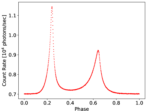
Figure 1: Crab pulsar’s FLC in the energy range $1-10$ keV from NICER having $1024$ phase bins.

Figure 1 shows the folded light curve (FLC) of the Crab Pulsar in the soft X-ray energy range $1-10$ keV, obtained by Vivekanand (2021) using the Neutron star Interior Composition Explorer (NICER) satellite observatory (Arzoumanian et al., 2014; Gendreau et al., 2016). It is similar to the FLC in Fig. $15$ of Vivekanand (2021) except that phase $0$ now represents the statistical minimum of the FLC, obtained by fitting a cubic polynomial to the first $275$ data of the earlier FLC. Visually it is conceivable that there is an approximate reflection symmetry between the two peaks in Fig. 1 provided their amplitudes are similar. Such a possibility has been evident to $\gamma$-ray astronomers in three of the brightest rotation powered pulsars (RPP) — Vela (Abdo et al., 2009), Crab (Abdo et al., 2010a) and Geminga (Abdo et al., 2010b), with Vela being the clearest example.

In the Vela pulsar’s $\gamma$-ray FLC Abdo et al. (2009) note that its two peaks are asymmetric, and that the second peak has a slow rise and a fast fall, and the first peak has the opposite behavior (see their Sect. $4.1$, page $1088$). Bai & Spitkovsky (2010) mention that Vela’s FLC has a horn structure that is symmetric upon reflection around the middle of the bridge (see their Sect. $5$, page $1292$). Abdo et al. (2010a) note in their Sect. $4.1$ on page $1257$ that the two peaks of the Crab pulsar’s $\gamma$-ray FLC are asymmetric, and that the second peak has a slow rise and a steeper fall. Saito (2010) notes that the rising and falling edges of the two peaks in the $\gamma$-ray FLC of the Crab behave exponentially, and that the slopes are not symmetric between the rising and falling edges (Sect. $7.3$, page $70$). Although Abdo et al. (2010b) do not specifically mention any asymmetry in the two peaks of the $\gamma$-ray FLC of the Geminga pulsar, the argument of Bai & Spitkovsky (2010) appears to hold for this RPP also (Fig. $2$ of Abdo et al. (2010b)). Cheng et al. (2000) note that in earlier $\gamma$-ray observations of these three pulsars from EGRET, the two peaks are not symmetric. In their Sect. $4.4$ on page $972$, Cheng et al. (2000) specifically mention that their simulations of the Crab pulsar’s FLC (in their Fig. $7$) have some sort of symmetry. Thus several astronomers have noted the apparent asymmetry between the two peaks in the $\gamma$-ray FLCs of these three RPPs, giving the impression of a reflection symmetry between the two peaks.

This work explores this aspect in Fig. 1 above, the focus being on the reflection symmetry between the rising edge of the first peak and the falling edge of the second peak. Comparison of the falling edge of the first peak and the rising edge of the second peak would be model dependent due to the bridge emission, and therefore has not been pursued here; this is elaborated upon later on.

The reflection symmetry noticed by earlier astronomers is essentially a visual effect. It was implied (in my opinion) over a phase range of the order of $\approx 0.2$ which would be approximately from phase $0$ to the first peak in Fig. 1. To the best of my knowledge no one has so far studied these issues quantitatively. This work attempts a quantitatively analysis of this subject and concludes that the reflection symmetry exists, if at all, only in a small phase range close to the two peaks. However one can believe it to exist over a much larger phase range if one is willing to accept the existence of a weak and broad emission component in the wings of the second peak.

An important requirement for this work is the highest possible phase resolution in Fig. 1 which has $1024$ phase bins per period, which is the highest currently available. This is possible because of the excellent photon collecting and timing ability of NICER. Vivekanand (2021) discusses the required accuracy on the rotation frequency of the Crab pulsar $\nu(t)$ and its time derivative $\dot{\nu}(t)$ as a function of epoch $t$, to obtain this phase resolution. Often $\gamma$-ray and X-ray FLCs of RPPs are obtained by using contemporaneous radio timing ephemeris. This should be good enough for most milli second pulsars whose $\nu(t)$ changes relatively slowly with epoch and which have low timing activity. However for the Crab pulsar the systematic differences between the $\nu(t)$ and $\dot{\nu}(t)$ estimated at radio and X-rays should be taken into account while forming high phase resolution FLC. The $\nu(t)$ and $\dot{\nu}(t)$ used to form Fig. 1 have been obtained self consistently from NICER data itself (Vivekanand, 2020), to yield an effective resolution of better than $1/512$ in phase (Vivekanand, 2021).

2 Observations and data analysis

The NICER observations of this work as well as their analysis have been described in detail by Vivekanand (2020, 2021) including data calibration and filtering.

Fig. 2 shows the rising edge of the first peak of Fig. 1 and the reflected version of the falling edge of the second peak, aligned such that their peaks lie at the same phase. The red curve in Fig. 2 is identical to samples $1$ to $253$ of the FLC in Fig. 1, while the blue curve is identical to samples $652$ to $1024$ after abscissa inversion; the peaks of the two curves at samples $248$ and $657$ respectively are aligned at phase $0.19921875$ in Fig. 2 (cyan line), and only a smaller portion of the curves has been plotted in the figure. The main effort in this work is to equalize the areas under the two curves so that their peak amplitudes are similar, and identify phase ranges where they match statistically. One searches for a good match in the space of four parameters: finer phase adjustment to the phase alignment of the two curves $\phi_{0}$; the initial and final phases of the phase range for matching $\phi_{1}$ and $\phi_{2}$; and a multiplicative correction to the relative area normalization of the two curves $\kappa$. This will be known as analysis without any smoothing of the red curve.

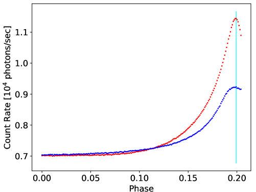
Figure 2: Superposition of the rising edge of the first peak (red) and reflected version of the falling edge of the second peak (blue), aligned at their peaks (cyan line which is at phase $0.19921875$).

However, Fig. 1 indicates that the second peak may be wider than the first peak. So the above analysis is repeated after convolving the red curve with a smoothing function. If the smoothing function is symmetric, like the Gaussian, an additional parameter is added to the search space, which is a measure of the width $\sigma$ of the smoothing function. This will be known as analysis with symmetric smoothing. If the smoothing function is asymmetric then two additional parameters are added to the search space, which are a measure of the widths $\sigma_{-}$ and $\sigma_{+}$ of the smoothing function on the negative and positive phase sides of its peak. This will be known as analysis with asymmetric smoothing.

3 Results of analysis without smoothing

Fig. 3 shows the best result when no smoothing is done. First the complete red and blue curves of Fig. 2 (this includes the portions not plotted) are adjusted to have zero photons/sec in their first sample; this will be known as baseline removal. Next the area under the red curve is made equal to that under the blue curve. Then the blue curve is shifted with respect to the red curve by minus one phase sample ($\phi_{0}=-1/1024$ cycles). Finally the red curve is multiplied by $\kappa=0.977$, and the range of matching is chosen to be $\phi_{1}=0.1616$ and $\phi_{2}=0.1860$. This data is plotted in the top panel of Fig. 3. The cyan line represents the new peak alignment that includes $\phi_{0}$ and the vertical orange lines represent $\phi_{1}$ and $\phi_{2}$. The difference of the blue and red curves is plotted in the bottom panel of Fig. 3. The $25$ data between $\phi_{1}$ and $\phi_{2}$ have a mean value of $-0.78\pm 1.8$ photons/sec, the reduced $\chi^{2}$ being $0.93$. Significantly better results are obtained if two outlying data at phases $0.1748$ and $0.1826$ are ignored; then the mean of the $23$ data is $1.12\pm 1.37$ and the reduced $\chi^{2}$ is $0.51$.

The analysis of this section begins with obtaining an initial set of the parameters $\phi_{0}$, $\phi_{1}$, $\phi_{2}$ and $\kappa$ by trial and error, for which the reduced $\chi^{2}$ is acceptable ($\leq 1.0$), ensuring that the initial range $\phi_{2}-\phi_{1}$ is as large as possible. Then three additional phase samples on either side of the initial range are utilized to create $16$ phase ranges for searching. So the start of the range would have any of the four phases $\phi_{1}-n/1024,n=0,1,2,3$, while the end of the range would have any of the four phases $\phi_{2}+n/1024,n=0,1,2,3$. For each of these $16$ ranges $21$ values of $\kappa$ are tried within the range $\pm 0.01$ about its initial value in units of $0.001$. Statistics of the difference between the red and blue curves of Fig. 3 are obtained for each of these $336$ combinations, both with and without the two outlying data.

To understand the reduced $\chi^{2}$ mentioned above, let $R_{i}$ and $B_{i}$ be the count rates of the red and blue curves respectively in the $i^{th}$ sample in Fig. 2. Let $r_{i}$ and $b_{i}$ be the corresponding errors, obtained from Poisson statistics and scaling, and let $R_{0}$ and $B_{0}$ be the count rates in the first sample of each curve; note that the red and blue curves in Fig. 2 have $254$ and $373$ samples although a smaller amount of this data is plotted in the figure. Let $A_{r}=\sum_{i}(R_{i}-R_{0})$ and $A_{b}=\sum_{i}(B_{i}-B_{0})$ be the sum of all red and blue samples respectively in Fig. 2, after removing the baseline from each curve. The blue curve in the top panel of Fig. 3 is $B_{i+1}-B_{0}$ where the subscript $i+1$ represents shift by minus one sample, while the red curve is $(R_{i}-R_{0})\kappa A_{b}/A_{r}$ after area normalization. The difference between the blue and red curves in the $i^{th}$ sample is $D_{i}=(B_{i+1}-B_{0})-(R_{i}-R_{0})\kappa A_{b}/A_{r}$.

Its error is $d_{i}=[b^{2}_{i+1}+r^{2}_{i}(\kappa A_{b}/A_{r})^{2}]^{1/2}$. Although $B_{0}$ and $R_{0}$ are counts in some phase samples, and have Poisson statistical errors on them, they do not contribute to $d_{i}$ because they are essentially constants for our purpose. To understand this, one should recall that each $d_{i}$ can be modeled as $\left[<D^{2}_{i}>-<D_{i}>^{2}\right]^{1/2}$ where $<>$ represents ensemble averaging. The set of ensemble $D_{i}$ for each phase sample $i$ are of course not available, since one has only one $D_{i}$ measurement for each $i$. However this formula brings out the fact that adding or subtracting a constant value to a statistical sample changes its mean but not its variance.

However this would not be the case if each phase sample $i$ had a different $B_{0}$ and $R_{0}$. Then their mean values will bias $D_{i}$ and not contribute to $d_{i}$ as before; but their statistical errors will contribute to $d_{i}$. For illustration consider observations of radio spectral lines using N radio frequency channels, in which observations are first done by centering the N channels on the spectral line plus continuum, then observations are done by centering them only on the continuum (say by frequency switching). The latter data are subtracted from the former channel by channel to obtain the spectral line, the noise on which depends upon the noise on the off-line channels also.

In summary, $B_{0}$ and $R_{0}$ behave like constants in the formula for $D_{i}$, being the same for all phase samples $i$. Their statistical errors bias each $D_{i}$ in the same manner and do not contribute to the corresponding $d_{i}$. Instead, if $B_{0}$ and $R_{0}$ were different for each phase sample $i$, then their errors would be reflected in each $b_{i}$.

Both $D_{i}$ and $d_{i}$ are plotted in the bottom panel of Fig. 3. The reduced $\chi^{2}$ is obtained by the formula $\sum_{i}^{N}(D_{i}/d_{i})^{2}/N$ where the sum is over all of the $N$ phase samples between $\phi_{1}$ and $\phi_{2}$. The error on the reduced $\chi^{2}$ is $\sqrt{2/N}$.

The red and blue curves of Fig. 2 have a good match in the phase range $\phi_{2}-\phi_{1}=0.1860-0.1616=0.0244$ after baseline removal, area normalization and phase shift; but this is a very small fraction of the phase range over which the reflection symmetry is implied. The bottom panel of Fig. 3 shows a broad and faint emission component of amplitude $\approx 100$ photons/sec and width $\approx 0.1$ in phase, centered at phase $\approx 0.1$ beyond the second peak of the FLC in Fig. 1, or equivalently before the second peak in the reflected FLC in Fig. 2. Only if this component is real can the reflection symmetry be believed to exist over a substantial phase range of $\approx 0.2$.

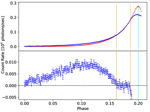
Figure 3: Top panel: Similar to Fig. 2 but after baseline removal, area normalization, shifting the blue curve by $\phi_{0}$ in phase, and multiplying the red curve by $\kappa$. Bottom panel: Difference of the blue and red curves. The orange lines represent $\phi_{1}$ and $\phi_{2}$.

4 Results of analysis with symmetric smoothing

Three symmetric smoothing functions were tried – Gaussian, Lorentzian and Laplace, the last being two exponential functions set back-to-back, its functional form being $f(x)=\exp(-|x|/\sigma)/(2\sigma)$. The Laplace smoothing gave the best results that are shown in Fig. 4; Gaussian and Lorentzian smoothing fared poorly in comparison.

The initial analysis of this section is similar to that of the previous section – removal of baseline of the red and blue curves, then their areas being made equal, then shifting the blue curve by minus one sample in phase ($\phi_{0}=-1/1024$). Then the red curve is convolved with a Laplace function having $\sigma=0.0039$. Now the convolution theorem states that convolution of two functions implies multiplying their Fourier transforms (Bracewell, 2000). So the red curve and a sampled Laplace function are set into zero padded data arrays $1024$ locations long, and the product of their complex Fourier transforms (obtained using FFT) is inverse Fourier transformed to obtain the smoothened curve. The smoothened curve is multiplied by $\kappa=0.959$ and the range of matching is chosen to be $\phi_{1}=0.1616$ and $\phi_{2}=0.1890$. This data is plotted in the top panel of Fig. 4.

The search space now consists of five parameters: $\phi_{0}$, $\phi_{1}$, $\phi_{2}$, $\kappa$ and $\sigma$. $\phi_{0}$ is set to minus one sample ($-1/1024$) as earlier. The $16$ combinations of ($\phi_{1},\phi_{2}$) are coupled with $41$ values of $\kappa$ between $0.94$ and $0.98$, and $60$ values of $\sigma$ between $0.0012$ and $0.0071$, yielding $39360$ estimations of the $\chi^{2}$.

Smoothing the red curve reduces the noise on it. Using the terminology of the previous section, the count rate in the $i^{th}$ sample of the red curve is $C_{i}=(R_{i}-R_{0})A_{b}/A_{r}$; its error is $c_{i}=r_{i}A_{b}/A_{r}$. Convolution is essentially a weighted average where the sum of the weights is unity: $F_{i}=\sum_{j=-N}^{N}w_{i-j}C_{i-j}/\sum_{j=-N}^{N}w_{i-j}=\sum_{j=-N}^{N}w_{i-j}C_{i-j}$; the weights $w_{i-j}$ are samples of the Laplace function that is centered on the $i^{th}$ sample, and $2N$ is some effective number of samples. The variance on $F_{i}$ is given by $f^{2}_{i}=\sum_{j=-N}^{N}w^{2}_{i-j}c^{2}_{i-j}$ which is merely the convolution of the scaled variance on the red curve $c^{2}$ with the square of the Laplace function $w^{2}$, after proper normalization for the area of the latter. So $f_{i}$ can also be derived using the convolution theorem. The $f_{i}$ thus estimated in the Fourier domain has been verified by comparing it with the $f_{i}$ computed explicitly in the time domain using the weighted sum formula above. $F$ and $f$ are plotted as the red curve and its error in Fig. 4 after multiplication by $\kappa$.

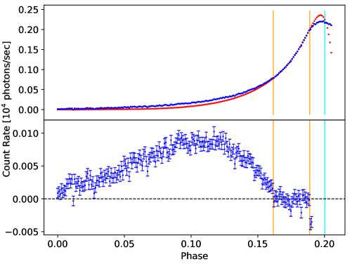
Figure 4: Similar to Fig. 3, except that the red curve here is the red curve of Fig. 3 after being convolved with a Laplace function.

The phase range of matching has now increased to $0.0274$ in Fig. 4. The mean value of these $28$ data is $-1.23\pm 1.30$ photons/sec, the reduced $\chi^{2}$ being $0.76$. If the above mentioned two outlier data are ignored the corresponding numbers are $0.20\pm 0.92$ and $0.35$ respectively, which is a significant improvement. So Laplace smoothing of the red curve increases the phase range of curve matching by three phase samples, as well as improves the statistical similarity of the two curves. Once again the difference between the red and blue curves is a broad and faint component similar to that seen in the bottom panel of Fig. 3.

Therefore, while smoothing with the Laplace function improves the match between the red and blue curves in Fig. 4, this is still a very small fraction of the phase range over which the reflection symmetry is implied.

5 Results of analysis with asymmetric smoothing

The analysis of the previous section was repeated by choosing asymmetric versions of the Gaussian, Lorentzian and Laplace functions for smoothing the red curve of Fig. 2. Asymmetric functions were tried to obtain better matching closer to the peaks than was obtained in Fig. 4, but this did not succeed. Fig. 5 is an example of one of the best results obtained in this section, and is similar to Fig. 4 except that the Laplace function has width $\sigma=0.0039$ at negative phases with respect to its peak and width $\alpha\times\sigma$ at positive phases with $\alpha=0.8$. In Fig. 5 $\phi_{0}=-1/1024$, $\phi_{1}=0.1616$ and $\phi_{2}=0.1890$ as in Fig. 4 but $\kappa=0.936$.

The search space now consists of six parameters: $\phi_{0}$, $\phi_{1}$, $\phi_{2}$, $\kappa$, $\sigma_{-}$ and $\sigma_{+}$. As usual $\phi_{0}$ was set to minus one sample ($-1/1024$). The $16$ combinations of ($\phi_{1},\phi_{2}$) were coupled with $41$ values of $\kappa$ and $60$ values of $\sigma_{-}$ and six values of $\alpha$ where $\sigma_{+}=\alpha\times\sigma_{-}$, $\alpha=0.9-0.5$ and $0.1$, yielding $16\times 41\times 60\times 6=236160$ estimations of the $\chi^{2}$. The ranges of $\kappa$ had to be chosen differently for different values of $\alpha$.

The phase range of matching $0.0274$ is similar to that in Fig. 4. The mean value of these $28$ data is $-0.76\pm 1.31$ photons/sec, the reduced $\chi^{2}$ being $0.76$. If the above mentioned two outlier data are ignored the corresponding numbers are $0.70\pm 0.91$, and $0.35$ respectively. The results of Fig. 5 are similar to those of Fig. 4 since moderate asymmetry is imposed upon the Laplace function. Asymmetric versions of Gaussian and Lorentzian functions fared poorly in comparison. The difference between the red and blue curves in Fig. 5 is similar to that in Fig. 4 or Fig. 3.

An asymmetric version of the Gaussian or Lorentzian was derived by multiplying with the odd function $1+\beta\phi$ where $\phi$ is the phase and the magnitude of $\beta$ can be chosen to control the level of asymmetry, while its sign controls the sense of the asymmetry. Any other odd function can be used such as $1+\beta\phi^{3}$. The asymmetry increases monotonically with $\beta$. Since the width of the smoothing functions is required to be of the order of $\approx 0.004$ for our data, large values of $\beta$ are required to achieve the required levels of asymmetry. This makes the smoothing function negative at larger $|\phi|$ values. These negative function values have to be removed but this makes the smoothing function discontinuous in its derivative.

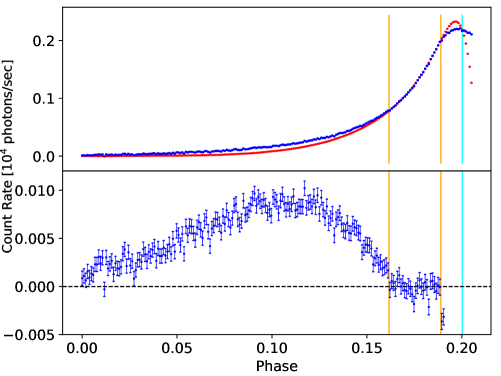
Figure 5: Similar to Fig. 4, except that the red curve here is the red curve of Fig. 3 after being convolved with an asymmetric Laplace function.

6 Discussion

In the introduction it was stated that comparison of the falling edge of the first peak and the rising edge of the second peak is model dependent due to the bridge emission. This is because the emission between the two peaks in Fig. 1 has to be modeled, at the minimum, as a falling edge of the first peak (say C1), a bridge emission (C2) and a rising edge of the second peak (C3), if one believes that there are two peaks in the FLC and if one is trying to study their mirror symmetry. Now, Fig. 1 gives the sum C1 + C2 + C3 between the two peaks, from which one has to obtain C1 and C3 to study their mirror symmetry. Clearly one has to model C1 and C2 to get C3, or C2 + C3 to get C1; either way the bridge emission C2 has to be modeled.

On the other hand, the visually suspected mirror symmetry discussed in this work is between the observed rising edge of the first peak and the observed falling edge of the second peak, irrespective of how many independent emission regions of the pulsar’s magnetosphere contribute to them, not to mention emission from the two independent magnetic poles also. So this work does not need to model these two data sets – it uses them directly.

An important point in this work is that it compares the red and blue curves when they are aligned at their peaks (almost!). This adds greater credence to any matching between the two curves, since one is not comparing arbitrary sections of two curves.

A different analysis to explore is when the phase range of comparison in Fig. 3 becomes $\phi_{1}=0.0$ and $\phi_{2}=0.1860$, which is approximately the phase range over which the reflection symmetry has been visually perceived; i.e., one wonders what happens when one attempts to minimize the reduced $\chi^{2}$ over almost entire phase range in Fig. 3. To differentiate from earlier results let this be called "entire $\chi^{2}$". The "entire $\chi^{2}$" values are $47.03,44.43,42.47,41.14,40.43,40.32,40.81,41.89,43.54,45.75$ and $48.51$, for values of $\kappa$ ranging from $0.96$ to $1.06$ in steps of $0.01$. At the specific value of $\kappa=0.977$ in Fig. 3 the "entire $\chi^{2}$" is $42.99$, while its minimum value is $40.29$ at $\kappa=1.006$. There is not much difference between "entire $\chi^{2}$" values of $42.99$ and $40.29$.

Fig. 6 is similar to Fig. 3 except that the phase range of comparison is much larger and $\kappa=1.006$. The broad and faint component below $\phi_{1}=0.1616$ persists, while the red and blue curves depart significantly from each other in the original phase range of comparison $\phi_{1}=0.1616$ and $\phi_{2}=0.1860$. This trend continues for $\kappa$ values departing significantly from $1.006$ – the two curves depart dramatically from each other in the original phase range of comparison, while the broad and faint component persists without significant changes. I believe this is because changes in $\kappa$ make much larger changes to the original matching phase interval, in which the light curve is changing almost exponentially, and make relatively smaller changes in the rest of the phase range in which the light curve is changing far more slowly.

The "entire $\chi^{2}$" analysis is probably for those who are interested in finding out what sort of minimal emission components exist on the falling edge of the second peak, probably for theoretical modeling. The motivation/philosophy of this work is quite different. It looks for the largest phase range of matching of the blue and red curves, not for the smallest statistical difference between the two.

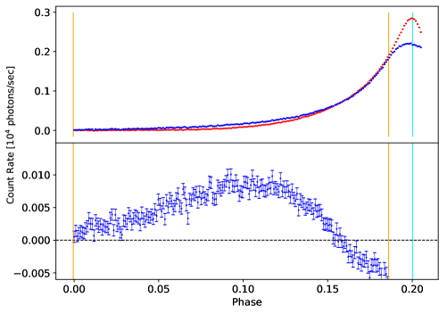
Figure 6: Similar to Fig. 3, except that the "entire $\chi^{2}$" is estimated in the phase range $\phi_{1}=0.0$ and $\phi_{2}=0.1860$, and $\kappa=1.006$.

The main result of this work is that strictly the visually apparent reflection symmetry in the FLC of the Crab pulsar is restricted to a very small phase range of $\approx 0.0274$, which is so small that one can not rule out a coincidental matching. The only way this can be extended to a substantial phase range is by invoking a broad and faint emission component beyond the second peak, that is shown in the bottom panels of figures 3, 4 and 5. Conversely, if in future the spectrum of this component turns out to be different from the rest of the FLC, then greater credence can be given to its existence; then one can believe that the reflection symmetry in the Crab pulsar’s FLC extends over a substantial phase range. Pending such confirmations, if at all, the rest of this section will speculate on the consequences of supposing that these two facts are true, because currently it is too early to reject the existence of the reflection symmetry.

6.1 Mirror symmetry

Throughout this work the stress has been on the "approximate reflection symmetry" between the rising edge of the first peak and the falling edge of the second peak of the Crab pulsar’s soft X-ray FLC. I believe earlier astronomers (both observers and theorists) also implied the same since theirs was essentially a visual observation. The concept of perfect reflection symmetry is non existent in the current work which is observational. Matching of segments of FLCs is subject to the noise on those segments and to the phase resolution of the data – today’s perfect matching may be overturned by tomorrow’s higher quality data that may have less noise and higher phase resolution. The important point here is that earlier astronomers were impressed with even the semblance of a reasonable reflection symmetry since the two edges are supposed to arise from widely different regions of the pulsar’s magnetosphere. Clearly earlier astronomers were reporting the zeroth order visual effect while visually smoothing out any higher order departures from perfect reflection symmetry.

Very early Cheng et al. (1986) and Romani & Yadigaroglu (1995) demonstrated the formation of double peaked $\gamma$ ray FLCs of RPPs using only a dipole magnetic field, special relativistic aberration and light travel time of a photon, without invoking the details of the radiative processes. It will be very convenient if the mirror symmetry of the two peaks is also explained using the above minimal inputs. Indeed figure $5$ of Romani & Yadigaroglu (1995) and Fig. $8$ of Cheng et al. (2000) show simulated light curves that rise steeply towards the first peak and fall as steeply after the second peak, but their phase resolution was much worse than that of this work. A priori one could suppose that the mirror symmetry can be explained more easily if the emission was from only one pole of the Crab pulsar instead of two poles, since there would be one parameter less to deal with. However, Tang et al. (2008) show in their Figure $6$ that the rising edge of the first peak of the Crab pulsar’s high energy FLC has significant contributions from both of its magnetic poles, while the falling edge of the second peak has significant contribution from only one pole. Moreover they invoke emission asymmetry between the two poles of the Crab pulsar since the dipole may not be at the center of the pulsar. These additional details may make the explanation for the mirror symmetry more complicated. So this mirror symmetry, if at all it exists, may be an important constraint for modeling the soft X-ray FLC of the Crab pulsar.

Several authors have simulated high energy FLCs of RPPs for diverse magnetic field structures and acceleration gaps under different magnetospheric and geometric assumptions (Venter, 2009; Watters, 2009; Romani & Watters, 2010; DeCesar, 2013; Kalapotharakos et al., 2014); these are known as light curve atlases. Some of these simulated FLCs do display some sort of reflection symmetry between the two peaks, although there are equal number which display only translation symmetry. These simulated FLCs depend critically upon the shape and size of the emission zone in the magnetosphere and the intensity weight for each point in this zone, i.e., the relative amount of radiation emitted from each point. Most authors make the simple assumption the intensity weight is uniform across the emission zone. The mirror symmetry may provide constraints upon the shape and size of the emission zone and the intensity weight within it.

That the mirror symmetry improves upon smoothing the data with a Laplace function is a surprising result; intuitively one might have expected a more common function like the Gaussian, which however fares poorly in comparison. This may be yet another critical constraint for the modeling of soft X-ray FLCs of RPPs.

6.2 Broad and faint emission component

To the best of my knowledge the broad and faint emission component in the Crab pulsar’s soft X-ray FLC has been reported for the first time in this work. It is not surprising that it was undetected so far. In Fig 1 the second peak occurs at phase $0.6431$ and the peak of the broad and faint emission component occurs at phase $\approx 0.6431+0.1\approx 0.7431$, where the FLC value is $\approx 7176$ photons/sec. Clearly a maximum FLC enhancement of $\approx 100/7176\approx 1.4$% is not discernible to the human eye in Fig 1, particularly since this component is riding on top of a curving wing of the second peak. Moreover, the sum of the count rates of this component in the bottom panel of Fig. 4 in the phase range $0-0.1616$ is $9078.01\pm 95.64$ photons/sec, while the corresponding number for the blue curve in the top panel of that figure is $1196851.36\pm 94.53$; so when this component is integrated it is only a fraction of $0.0076\pm 0.00008$ or $\approx 0.76$% $\pm 0.01$% of the background that it is riding on. Therefore it is not surprising that this component was not evident in the earlier soft X-ray FLCs of the Crab pulsar that had lower sensitivity and resolution and became evident only after the quantitative analysis of this work. If this component is indeed real then its nature may be revealed when its spectrum is obtained, but that may be difficult due to its faintness. Meanwhile we can make the following speculations.

The Crab pulsar’s radio FLC has seven components (Eilek & Hankins, 2016) some of which are prominent only at higher radio frequencies (beyond $\approx 5$ GHz). The positions of two of these labeled HFC1 and HFC2 drift in rotation phase as a function of observing radio frequency, and appear at higher phases at higher radio frequencies. See Fig $1$ of Eilek & Hankins (2016) who state that there is no clear sign of these two components in high energy FLCs of the Crab pulsar, except for a possible weak detection above $\approx 10$ GeV by Abdo et al. (2010a), who detect a slight enhancement in the FLC in their Fig. $1$ at phase $\approx 0.74$. Now the second peak in their figure is at phase $\approx 0.39$. So the faint feature detected by Abdo et al. (2010a) lies at phase $\approx 0.35$ beyond the second peak, while the feature detected here lies phase $\approx 0.1$ beyond the second peak. Moreover, the width of the feature of Abdo et al. (2010a) is much narrower compared to the feature here. Therefore it appears unlikely that the two are connected although it should be kept in mind that the two measurements are at widely different energies. Nevertheless it is interesting to speculate if the broad and faint feature detected here is in some way connected to the radio HFC1 and HFC2 components of the Crab pulsar, particularly if their high energy counterparts also drift in phase.

If the spectrum of this broad and faint component turns out to be completely non thermal, then it would have to be explained by the standard light curve modeling done at high energies (Bai & Spitkovsky, 2010; Romani & Watters, 2010; Harding, 2016). Figure $6$ of Tang et al. (2008) demonstrates a possibility – a broad and weak extended emission beyond the second peak that arises due to widening of the azimuthal extension of the outer gap. However their component decreases monotonically with phase beyond the second peak while the feature hear peaks at phase $\approx 0.1$ beyond the second peak.

If the spectrum of this broad and faint component turns out to be thermal, then there are interesting possibilities – it would point to a thermal hot spot on the surface of the Crab pulsar. It would be more interesting if it turns out to be like the spectrum of a magnetar, which is a combination of a thermal and two non thermal components, the former arising from a surface hot spot while the latter is due to the magnetic atmosphere of the pulsar; see Fig. $3$ of Mereghetti et al. (2015), Fig. $5$ of Kaspi & Beloborodov (2017) and Fig. $2$ of Esposito et al. (2020). This would indicate that there is a bit of a magnetar behavior in the Crab pulsar. This would be consistent with the assertion of Esposito et al. (2020) in their final remarks that magnetars can be radio pulsars and ordinary radio pulsars can behave like magnetars. This would also be consistent with the relatively high rate of glitch and timing noise activity in the Crab pulsar, which is a typical magnetar behavior (Turolla et al., 2015; Kaspi & Kramer, 2016; Esposito et al., 2020).

7 Data availability

The data underlying this article are available at the NICER observatory site at HEASARC (NASA). The data of Fig. 1 is available in the article’s online supplementary material.

References

- Abdo et al. (2009) Abdo, A.A., Ackermann, M., Atwood, W.B. et al. 2009, ApJ, 696, 1084
- Abdo et al. (2010a) Abdo, A.A., Ackermann, M., Ajello, M. et al. 2010, ApJ, 708, 1254
- Abdo et al. (2010b) Abdo, A.A., Ackermann, M., Ajello, M. et al. 2010, ApJ, 720, 272
- Arzoumanian et al. (2014) Arzoumanian, Z., Gendreau, K.C., Baker, C.L., et al. 2014, Proc. SPIE, 9144, 914420
- Bracewell (2000) Bracewell, R.N. 2000, "The Fourier Transform and its Applications", edition, McGraw Hill, Boston
- Bai & Spitkovsky (2010) Bai, X.N., Spitkovsky, A., 2010, ApJ, 715, 1282
- Cheng et al. (1986) Cheng, K.S., Ho, C. & Ruderman, M. 1986, ApJ, 300, 500
- Cheng et al. (2000) Cheng, K.S., Ruderman, M. & Zhang, L. 2000, ApJ, 537, 964
- DeCesar (2013) DeCesar, M.E. 2013, PhD thesis, University of Maryland.
- Eilek & Hankins (2016) Eilek, J.A., Hankins, T.H. 2016, J. Plasma Phys., 82, 635820302
- Esposito et al. (2020) Esposito, P., Rea, N., Israel, G.L. 2020, Review to appear in T. Belloni, M. Mendez, C. Zhang, editors, "Timing Neutron Stars: Pulsations, Oscillations and Explosions", ASSL, Springer
- Gendreau et al. (2016) Gendreau, K., Arzoumanian, Z., Adkins, P.W., et al. 2016, Proc. SPIE, 9905, 99051H
- Harding (2016) Harding, A. 2016, J. Plasma Phys. 82, 635820306
- Kalapotharakos et al. (2014) Kalapotharakos, C., Harding, A.K., & Kazanas, D. 2014, ApJ, 793, 97
- Kaspi & Kramer (2016) Kaspi, V.M. & Kramer, M. 2016, IJMP(d), 1, 22
- Kaspi & Beloborodov (2017) Kaspi, V.M. & Beloborodov, A.M. 2017, ARA&A, 55, 261
- Mereghetti et al. (2015) Mereghetti, S., Pons, J.A., Melatos, A. 2015, Space Sci Rev, 191, 315, DOI 10.1007/s11214-015-0146-y
- Romani & Yadigaroglu (1995) Romani, R.W. & Yadigaroglu, I.A. 1995, ApJ, 438, 314
- Romani & Watters (2010) Romani, R.W. & Watters, K.P. 2010, ApJ, 714, 810
- Saito (2010) Saito, T. 2010, Thesis, Ludwig–Maximilians University, Munich.
- Tang et al. (2008) Tang, A.P.S., Takata, J., Jia, J.J., Cheng, K.S. 2008, ApJ, 676, 562
- Turolla et al. (2015) Turolla, R., Zane, S., Watts, A.L. 2015, Rep. Prog. Phys., 78, 116901
- Venter (2009) Venter, C., Harding, A.K., Guillemot, L. 2009, ApJ, 707, 800
- Vivekanand (2020) Vivekanand, M. 2020, A&A, 633, A57
- Vivekanand (2021) Vivekanand, M. 2021, A&A, 649, A140
- Watters (2009) Watters, K.P., Romani, R.W., Weltevrede, P., Johnston, S. 2009, A&A, 695, 1289