Collaborative Multi-Radars Tracking by Distributed Auctions

Abstract

In this paper, we present an algorithm which lies in the domain of task allocation for a set of static autonomous radars with rotating antennas. It allows a set of radars to allocate in a fully decentralized way a set of active tracking tasks according to their location, considering that a target can be tracked by several radars, in order to improve accuracy with which the target is tracked. The allocation algorithm proceeds through a collaborative and fully decentralized auction protocol, using a collaborative auction protocol (Consensus Based Bundle Auction algorithm). Our algorithm is based on a double use of our allocation protocol among the radars. The latter begin by allocating targets, then launch a second round of allocation if they have resources left, in order to improve accuracy on targets already tracked. Our algorithm is also able to adapt to dynamism, i.e. to take into account the fact that the targets are moving and that the radar(s) most suitable for Tracking them changes as the mission progresses. To do this, the algorithm is restarted on a regular basis, to ensure that a bid made by a radar can decrease when the target moves away from it. Since our algorithm is based on collaborative auctions, it does not plan the following rounds, assuming that the targets are not predictable enough for this. Our algorithm is however based on radars capable of anticipating the positions of short-term targets, thanks to a Kalman filter. The algorithm will be illustrated based on a multi-radar tracking scenario where the radars, autonomous, must follow a set of targets in order to reduce the position uncertainty of the targets. Standby aspects will not be considered in this scenario. It is assumed that the radars can pick up targets in active pursuit, with an area of uncertainty corresponding to their distance.

Keywords: Collaborative combat· Distributed Auctions· Multi-Radar Tracker.

Presentation of the problem of collaborative multi-radar tracking

It is considered that each radar has a 2-dimensional frame in a polar coordinate system centered on itself. It is estimated that the influence of elevation is negligible, so it is not useful to use a 3-dimensional landmark.

Each target therefore has a position in the radar reference frame determined by its distance, denoted , and its azimuth (polar angle), denoted $\theta$ . The precision of the measurement made by the radar is noted: $\sigma_{r}$ in distance and $\sigma_{\theta}$ in azimuth. The resulting measurement uncertainty is represented as an ellipse. The measure itself corresponds to acentered 2-dimensional Gaussian random variable of covariance $K=R(\theta)\begin{pmatrix}\sigma_{r}&0\\ 0&\sigma_{\theta}\\ \end{pmatrix}$ , where represents the $R\left(\theta\right)$ angle $\theta$ rotation matrix. During active tracking, the aim is therefore to anticipate the next measurement to be performed on the target given the past of the target and its current position thanks to the use of a Kalman filter. As for the measurement, there is also a prediction uncertainty. This is summarized in fig. 1 with the measurement uncertainty in orange and the prediction uncertainty associated with the tracking of the target by the radar in purple.

The signal received by the radar is assumed to be subject to Gaussian white noise. The signal to noise ratio (S/N) is assumed to be constant. The value was set at 13, which corresponds to a common value in practice. The S/N will influence the standard deviation of the measurement. The S/N will in fact correspond to the quality of the output desired by the user. For a given S/N it is possible to choose the parameters such as the wavelength to be transmitted or the transmission power, etc.

We first start by formalizing the problem we are dealing with. We are interested in the multi-radar target allocation problem. We first describe the radar model. We then formalize the single-radar allocation problem, i.e. the problem where each target is tracked by at most one radar, and finally the complete multi-radar allocation problem, where each target can be tracked by up to two radars.

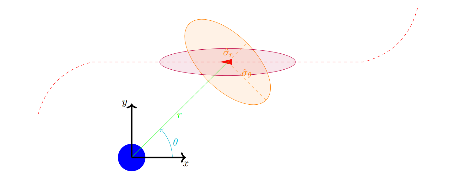
Figure 1: Illustration of uncertainty ellipses during active pursuit

First problem: mono-sensor allocation

It may be noted that the model described below corresponds exactly to a variant of a backpack problem. This problem can be formalized as follows:

$$\left(P1\right):\left\{\begin{aligned} \max\sum_{i,j}{c_{ij}\cdot x_{ij}}\\ \text{s.t.:}\\ \sum_{i}x_{ij}\leq 1,&\forall j\in\mathcal{J}&(C1)\\ \sum_{j}\gamma_{{ij}}\cdot x_{{ij}}\leq L_{t_{i}},&\forall i\in\mathcal{I}&(L)\\ x_{{ij}}\in\left\{0,1\right\},&\forall\left(i,j\right)\in\mathcal{I}\times\mathcal{J}\\ \end{aligned}\right.$$

Sets :

• $\mathcal{I}$ : Set of cardinality radars$|\mathcal{I}|=N_{u}$

• $\mathcal{J}$ : Set of cardinality tasks$|\mathcal{J}|=N_{t}$

Note that we are placed here, in the framework $\mathcal{I}\ll\mathcal{J}$.

The variables :

• $c_{{ij}}$ : Corresponds to the utility that the radar $i$ provides to the system if it handles the task $j$. $c_{{ij}}$ is of the following form, with $V(\mathcal{E}_{{ij}})$ the surface of the ellipse $\mathcal{E}_{{ij}}$ described by the Kalman filter matrix $P_{{ij}}$ of the radar $i$ for the target $j$:

  $$c_{{ij}}=f(V(\mathcal{E}_{{ij}}))$$

  Note that the function $f$ is therefore decreasing according to $V(\mathcal{E}_{{ij}})$.

• $x_{{ij}}$ : Boolean variable, $x_{{ij}}$ equals $1$ if the radar $i$ performs the task $j$ , 0 otherwise.

• $\gamma_{{ij}}$ : Cost of the task $j$ for the radar $i$.

• ${L_{t}}_{i}$ : Radar budget $i$.

Constraints :

• Constraint (C1) implies that a task can only be performed by a single radar.

• The constraint (L) models the load of the radar which must not exceed its budget. The $\gamma_{{ij}}$ are therefore similar to costs.

Let be a total of $|\mathcal{I}|+|\mathcal{J}|$ constraints.

Second problem: multi-sensor allocation

$$\left(P2\right):\left\{\begin{aligned} \max\sum_{i,j,k}{c_{{ikj}}\cdot w_{{ikj}}}\\ \text{s.t.:}\\ w_{{ikj}}={x_{M}}_{{ij}}\land x_{O_{{kj}}},\forall\left(i,k\right)\in\mathcal{I}^{2},\\ \forall j\in\mathcal{J}(A_{{ikj}})\\ \sum_{i}w_{{ij}}\leq 1,\forall j\mathcal{\in J}(C2)\\ \sum_{j}\gamma_{{ij}}\cdot({x_{M}}_{{ij}}+x_{O_{{kj}}}-w_{{iij}})\leq L_{t_{i}},\\ \forall i\in\mathcal{I}(L)\\ \left({x_{M}}_{{ij}},x_{O_{{kj}}}\right)\in\left\{0,1\right\}^{2},\forall\left(i,j\right)\mathcal{\in I\times J}\\ w_{{ikj}}\in\left\{0,1\right\},\forall\left(i,k\right)\in\mathcal{I}^{2},\forall j\mathcal{\in J}\\ \end{aligned}\right.$$

The variables :

• $c_{ikj}$ : Corresponds to the utility that the radar $i$ and the radar $k$ provide to the system if the radar $i$ handles the task $j$ as a main radar and $k$ as an optional radar. $c_{ikj}$ is of the following form, with $V(\mathcal{E}_{ij})$ (respectively $V(\mathcal{E}_{kj})$) the surface of the ellipse $\mathcal{E}_{ij}$ ( resp . $\mathcal{E}_{kj}$) described by the matrix $P_{ij}$ (resp. $P_{kj}$) of the Kalman filter of the radar $i$ (resp. $k$) for the target $j$ and $V(\mathcal{E}_{ij}\cap\mathcal{E}_{kj})$ the intersection volume of these two ellipses, as represented on LABEL:fig-reconciliation-ellipse:

$$c_{ikj}=f(V(\mathcal{E}_{ij}))+\alpha g(V(\mathcal{E}_{ij}\cap\mathcal{E}_{kj}))$$

$$\left\{\begin{matrix}f(V(\mathcal{E}_{ij}))>>\alpha g(V(\mathcal{E}_{ij}\cap\mathcal{E}_{kj}))\\ \alpha g\left(V\left(\mathcal{E}_{ij}\cap\mathcal{E}_{kj}\right)\right)>\varepsilon_{\min},\varepsilon_{\min}\in\mathds{R}_{*}^{+},\text{si }\mathcal{E}_{ij}\cap\mathcal{E}_{kj}\neq\varnothing\\ \end{matrix}\right.$$

where:

• ${x_{M}}_{{ij}}$ : Boolean variable, ${x_{M}}_{{ij}}$ equals $1$ if the radar $i$ performs the task $j$ as the main radar, 0 otherwise.

• ${x_{O}}_{{ij}}$ : Boolean variable, ${x_{O}}_{{ij}}$ equals $1$ if the radar $i$ performs the task $j$ as an optional radar, 0 otherwise.

• $w_{{ikj}}$ : Boolean variable, $w_{{ikj}}$ equals $1$ if the radar $i$ performs the task $j$ as main radar and the radar $k$ performs the task $j$ as optional radar, 0 otherwise.

Constraints:

• ($A_{ikj}$):Constraints making it possible to interface between the objective function and the other constraints according to the category of the task for the radar. The operator $\wedge$ corresponds to the logical AND operator. The constraint summarized here is equivalent to the two constraints below:

  $$\begin{matrix}&{x_{M}}_{{ij}}+{x_{O}}_{{ij}}-2w_{{ikj}}\leq 1\\ &{x_{M}}_{{ij}}+{x_{O}}_{{ij}}-2w_{{ikj}}\geq 0\\ \end{matrix}$$

  It may be interesting to note that if $w_{iij}=1$ then, it is considered that the task is only performed by a single main radar.

• $(C2)$ : This constraint corresponds to the constraint $(C1)$ of the first model. It lists all possible combinations of 2 sensors that track a target $j$. There is at most only one combination of sensors that can be chosen.

• $(L)$ : Just like the constraint $(L)$ of , this constraint models the load of the radar. If the radar is tracking the target as main or optional radar, the term between parentheses equals 1, otherwise it equals 0 and the load for the task is therefore not considered.

Let be a total of $|\mathcal{I}|^{2}\cdot|\mathcal{J}|+|\mathcal{J}|+|\mathcal{I}|$ constraints.

Note that the present formulation is difficult to generalize to a coupling of $n$ sensors, because it requires adding $n-1$ additional indices which would increase the number of constraints and Boolean variables far too much. Moreover, this would make the problem insoluble for a classical solver. However, it is estimated that in our case, two sensors are more than enough to have a significant precision on the target.

Adaptation of distributed auctions algorithms for multi-radar tracking

The approach that we present in this article is based on the use of two successive CBBA algorithms: the first to make an allocation as the main radar, the second as an optional radar. In this section, we proceed in two steps. We first present the CBBA algorithm and the adaptations we have made to it so that it can consider the specificities of radars. We then present the general process, which includes the CBBA algorithm, allows to consider the interactions between radars and the dynamism of the mission.

4.1 Adaptation of CBBA to radars

The CBBA (Consensus Based Bundle Auction) algorithm [1] is based on the communication between the different radars. The messages that the radars send to each other can be represented as a set of vectors. The set of vectors that a radar sends to another one corresponds to its current knowledge of the system. Using these messages, and therefore the knowledge of the other speed cameras, each speed camera can update its knowledge and transmit it in turn. The transmitted data includes:

• $Y$, the vector that contains the known winning bid utility for each target. For a radar $i$ , $Y=\left(y_{{ij}}\right)_{j\leq|T|}$

• $Z$, the vector that contains the identity of the radar that won the auction for each target. For a radar $i$ , $Z=\left(z_{{ij}}\right)_{j\leq|T|}$. Thus, by making the link with $Y$ , if we have $Z_{j}=i^{*}$ , then we know that it is the radar $i^{*}$ which made a winning bid of an amount $Y_{j}$

• $S$, which corresponds to a “timestamp” vector, it makes it possible to manage conflicts by making it possible to keep the track of the contacts between radars. For a radar $i$, $S_{i}=\left(s_{{ik}}\right)_{k\leq|A|}$. Each component therefore corresponds to the date of the last message received from each radar. It therefore makes it possible to determine which of 2 radars was the last to be in contact with another one and therefore to select the most up-to-date information. This vector is updated when an agent receives a message. The values of the agent’s neighbors are updated with the current time, while the values of other agents are updated with the most recent time of the agent’s neighbors:

$$s_{{ik}}=\left\{\begin{matrix}reception\ time\text{ if }k\in i.\\ \max_{l\in i.}s_{{lk}}\\ \end{matrix}\right.$$

In our case, for the allocation as main radar, another vector will also be sent. This is the vector $E=\left(e_{{ij}}\right)_{j\leq|T|}$ that groups the ellipses leading to the winning bids for each target. This notably makes it possible to calculate intersections with the latter.

The algorithm is divided into 2 main phases:

• A selection phase: the radar calculates the utility for each of the targets it can process. It then selects targets for which it has utility greater than the winning bid, until it cannot add any more due to overload, until there are no more targets it can deal, or that the proposed bids are too low.

• An update phase: the radar will open the messages it has received containing the knowledge of other radars and update its own according to rules defined in the form of a table (taken from the article on the CBBA), represented on LABEL:cbba-update.

The actions shown in the table are as follows:

• leave unchanged: $Y_{i}$ and $Z_{i}$ both remain unchanged

• update: $y_{{ij}}\leftarrow y_{{kj}}$ , $z_{{ij}}\leftarrow z_{{kj}}$ ,$e_{{ij}}\leftarrow e_{{kj}}$ ,

• reset: $y_{{ij}}\leftarrow 0$ , $z_{{ij}}\leftarrow\emptyset$ , $e_{{ij}}\leftarrow\emptyset$

In the static case, when all the radars have the same beliefs, we say that the consensus is established. That is to say that a distributed allocation conflict-free could be found; this therefore constitutes the end of the algorithm.

The CBBA algorithm has a 50% performance guarantee, i.e., in the worst case, the global solution obtained is greater than half of the optimal solution. Certain assumptions are necessary to ensure this convergence, the main one being the Diminishing Marginal Gain (DMG) constraint. We note $b_{i}$ all the tasks allocated to the radar $i$. The DMG constraint is as follows:

$c_{{ij}}=c_{{ij}}\left(b_{i}\right)\geq c_{{ij}}\left(b_{i}\oplus b\right)\forall b$ (DMG)

The constraint (DMG) reflects the fact that the utility for the same target must be decreasing in the number of tasks.

In our case, we also want to balance the loads of the radars, i.e., to make sure that a single radar will not take the maximum of tasks while leaving the others unoccupied. To respect this constraint, we added a bias:

$$c_{{ij}}^{\text{CBBA}}=\frac{c_{{ij}}}{|b_{i}|}$$

4.2 General loop, interaction and dynamism

The algorithm operates in a closed loop, where the algorithm is executed at each time step; in particular, the agent makes an allocation as the main radar, then it makes the allocation as an optional radar if it has remaining budget. Each allocation is made through a CBBA algorithm, and therefore includes the two phases of the algorithm (auction and consensus) explained above. It therefore receives and sends information on its allocation as main and optional radar at each time step. The dynamism aspect, which completes the global loop of the algorithm, is explained below.

The interactive aspect can be understood in the following way: on the one hand, a radar does not take into consideration the targets which it follows as main radar in the list of targets which it can take as secondary radar (that wouldn’t matter). On the other hand, the ellipses sent by the radars are taken into account by the other radars (whether they are ellipses sent directly by the neighbors of the radar or transmitted with the winning bids step by step). It is these ellipses which make it possible to perform the utility calculation for the allocation as a secondary radar, and which therefore make it possible to calculate the utility function of the radar for the target. Another aspect of coupling is how the budget is managed. Indeed, when the agent arrives at the stage of allocation as main radar, it considers its budget as all of its remaining budget plus the budget allocated as optional radar. If ever a new allocation as main radar is possible, it deallocates the tasks as optional radar with the lowest utility, and performs a reset as described in the previous section.

To take account of the dynamic aspect of our problem, we only considered that the consensus was never reached. Thus, all auctions concerning a target are not considered closed unless the target in question has not been seen throughout the system for a certain period of time. This delay must take into account the fact that all the radars of the system are not in direct communication. After this delay, the radar deletes the knowledge (which has become useless) that it had on the target and transmits the information. In the case where the target can be perceived again by the system, the latter behaves in the same way as for the appearance of a new target, namely that it creates the knowledge associated with it. After each allocation step (as main radar and optional radar), the latter performs the tasks to which it has allocated itself.

So the general loop (repeated forever) is as follows.

1. The radar makes the selection step as the main radar. To do this, it calculates the uncertainty ellipses for each target, and its utility function; it also applies the Kalman filters of all the targets it is already tracking.

2. If it has remaining radar time budget, the radar proceeds to the selection step as an optional radar on all the targets that are not already tracked as the main radar (with its remaining budget).

3. The radar proceeds to the consensus stage as the primary radar. The vectors $Y,Z,E$ and $S$ as main radars are updated; vectors are sent to neighbors.

4. The radar then proceeds to the consensus stage as an optional radar. Vectors $Y,Z$ and $S$ as optional radars are updated; vectors are sent to neighbors.

5. The radar tracks the targets it has selected, possibly by applying its Kalman filter.

Note that since the radar initiates the tracks at each execution of the two phases of CBBA, which means that the algorithm does not have time to converge. In practice, this can result in conflicts. This is the case for a target on the edge between two radars, and which is increasingly threatening. In this case, each radar making its decision on a previous value of the utility of the others, and its own current value, it will consider that its bid wins the bet. Similarly, a less and less threatening radar (i.e., whose usefulness decreases) will potentially be followed by no one, each radar considering that the other has a better bid than itself. Differentiation from conventional methods

The method we propose calls into question several classic points in target allocation. If there is indeed a method of target allocation by auction, our approach proposes a different method, where the role of the auctioneer is in fact distributed on the radars. The latter therefore hold two roles at once: that of bidder first, and then that of auctioneer. This feature is represented by the two phases of the algorithm: the auction phase and the consensus phase.

Another particularity of our approach is that it allows to allocate a target to several radars, thus making it possible to take advantage of the intersection of the ellipses of uncertainties generated by the different radars, which is not possible in the methods offered in the state of the art. Finally, we propose a classic auction, and not a combinatorial auction. While traditional auctions are generally less efficient than the combinatorial auctions described in the state of the art, they are also much faster, which allows our approach to achieve a relatively rapid allocation, particularly in a context where targets are move quickly.

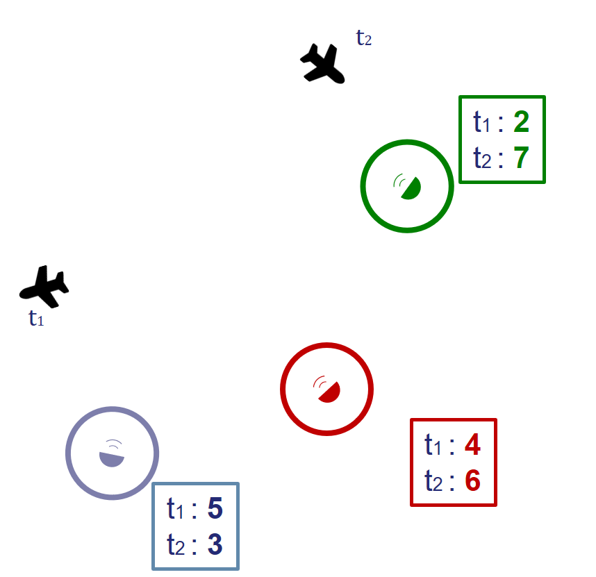
(a) initial allocation

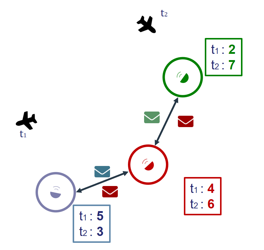
(b) sending messages

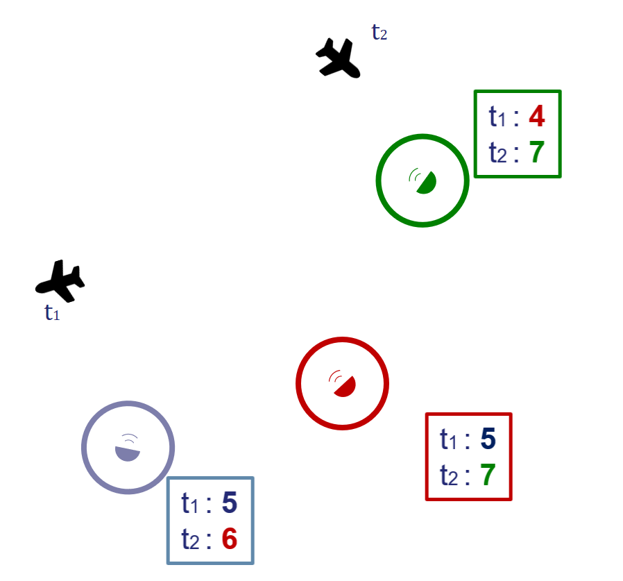
(c) Update (consensus)

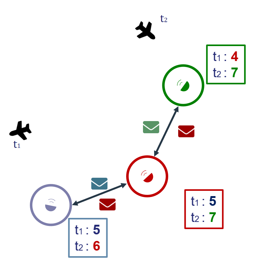
(d) Bidding & sending messages

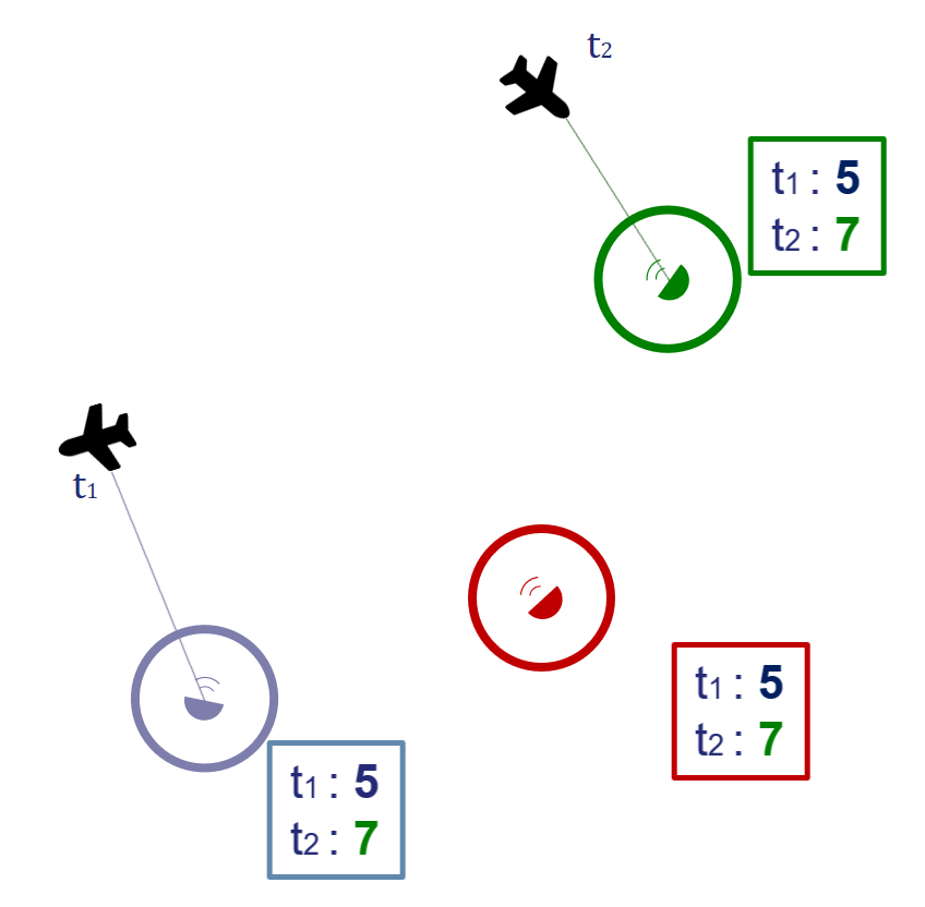
(e) Second consensus stage, consensus reached

Figure 2: Master Allocation Method Workflow for Two Targets and Three Radars

Algorithm illustration

Our approach makes it possible to solve the task allocation problem in an advantageous way: in the case where the radars remain in contact, even if the communication graph evolves during the mission, this remains possible provided that the graph of connection of the radars remains connected by arc. The total decentralization of the algorithm makes it possible to relax the constraint on the communication graph, which does not require having a radar in direct communication with all the radars, the information propagating in the communication graph. In order to make the allocation in a reasonable time, the calculations of allocation on the targets are done in an additive manner at the level of each radar, which makes it possible to reduce the combination thereof. Finally, by carrying out two sequential auction runs, our algorithm also takes into account the possible overlapping of uncertainty ellipses, and thus makes it possible to generate an allocation favoring more precise tracking of targets when possible, while prioritizing the tracking of as many targets as possible (depending on radar capability).

The main means of realization is the deployment of the CBBA algorithm on radars. To proceed with this deployment, each radar is provided with a part of the implementation of the utility function, which allows it to determine the utility associated with a target, as well as a decision function which allows it:

1. To bid on the targets it has detected during its standby phase, considering its own load limits,

2. To receive messages sent by other radars,

3. To calculate the winner for each target according to Table 1,

4. Return the updated table.

Radars must also be able to differentiate between first-round allocation messages – one that tracks as many targets as possible – and one that improves accuracy by generating an intersection of uncertainty ellipses. Each radar $i$ proceeds by trying to maximize $\sum_{j}{x_{{ij}}\cdot}c_{{ij}}$ for the main allocation (resp.$\sum_{j,k}{w_{{ikj}}\cdot}c_{{ikj}}$ for the optional allocation), that is to say the sum of the utilities corresponding to the targets that it tracks, while taking into account the information received from the other radars, in particular the bids made by the latter.

An example of the way the algorithm works for allocation of the main radar is represented on fig. 3. The implementation must also include an additional target disambiguation mechanism, making it possible to identify the targets present at several radars, and in particular a plot merging algorithm, making it possible to match the targets of the different radars. This induces the sending of additional information enabling this operation to be carried out, such as the estimated speed and position of the targets.

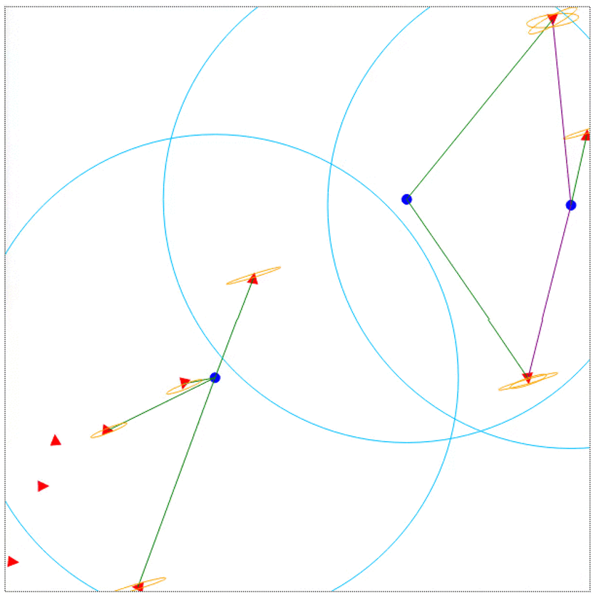
Figure 3: Simulation of the algorithm with 3 radars, the area where they are able to pick up targets in active pursuit, and 10 targets. The main track is in green, the secondary track in purple.

Results

The implementation of our model has been performed on the MESA framework [2], along with the Kalman filter package [3], on the same simulator as the one used in [4]. The fig. 3 shows the simulator: the radars are represented as blue points while the targets are represented as red triangles. Main radars following a target are represented as green lines, optional ones as purple lines. The uncertainty ellipses are in yellow.

In order to evaluate our work, we compare it to an optimal allocation, performed with the Coin-OR Branch and Cut tool (CBC). Results are represented on fig. 4. The blue (or green) curves correspond to the decentralized (or centralized) approach. The average value of each of the simulations and the different scenarios for a certain “composition” of Targets and Radars are presented. Each of the “compositions” of Targets and Radars is represented on the x-axis as a tuple (Targets, Radars). This allows us to compare the performance of the centralized and decentralized approaches with equivalent configuration. The colors of the bars correspond to the decentralized (D) or centralized (C) values, with optional tracking represented in light colors when relevant. The standard error (in black) is available for each of the bars of the different graphs.

Regarding the utility, as shown in the previous figure, the centralized approach obtains results superior to the decentralized approach. However, it can be seen that here too, for the decentralized approach, we obtain a utility clearly higher than the theoretical 50% of the CBBA algorithm compared to the centralized approach.

Regarding the coverage, we notice that for a constant configuration we obtain equivalent coverage in “main” tracking. The coverage being weaker for the coverage for the “optional” tracking.

Regarding the average load, we observe that for the configurations studied, there is almost no difference between the centralized and decentralized approaches. While we would have liked the decentralized approach should have a much lower load than the centralized approach.

As we can see overall, there are only very small differences between the centralized and decentralized approaches. This can be interpreted as a strength for the decentralized approach, because the radar configuration could then be adaptive (one could suppose that the radars are not fixed but can move) but also resilient, i.e., the global system could continue to function normally if a connection is cut, which is not the case with a centralized approach since there is only one connection with the control center. Since the load is also more evenly distributed, it can be assumed that the centralized approach can cope with a “surprise” attack without a total re-planning, which is not the case for the centralized approach. It should be noted that no experiment has been done with a higher number of radars since the constraint of the cost of purchasing a set of radars can be very limiting.

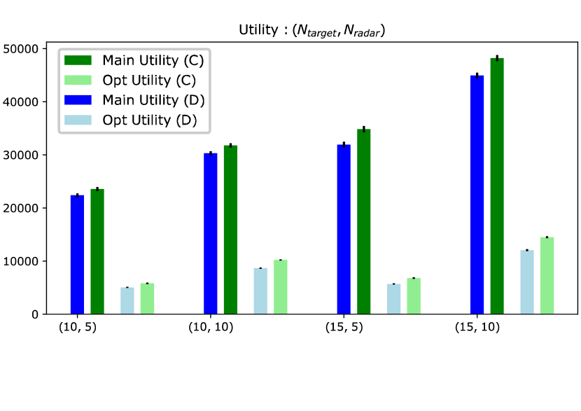
(a) Utility

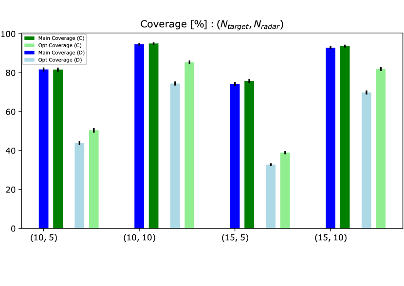
(b) Coverage

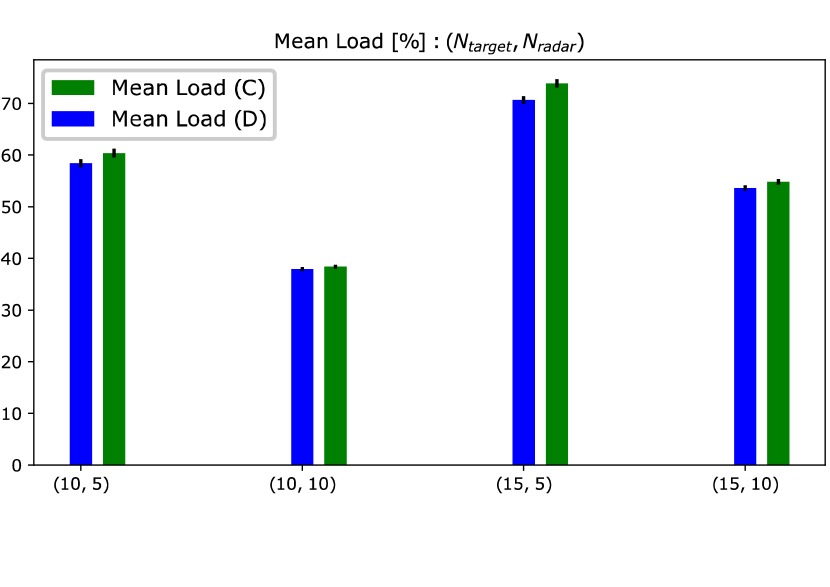
(c) Mean Load of the radars

Figure 4: Evolution of tracking metrics over scenarios generated randomly

Related works

Several works have focused on the use of decentralized approaches for task allocation for sensor, since the seminal work of Lesser et at. [5]. Since then, many approaches have been used. Recently, for real time use cases, auction methods have gained much interest in the multi-agent community [6, 7] for their capacity to perform good allocation in an affordable time. Many methods have been using auctions since then to allocate tasks in real-time, including to robots, sensors and radars (see for instance [8]).

One of the most successful recent algorithms is CBBA [1]. This algorithm allows to perform the allocation in a fully decentralized way, the agents acting both as auctioneers and bidders. This algorithm has since been used several times for sensors [9, 10]. However, none of them has been taking into account the specificities of radars, i.e., their collaboration through the intersection of their uncertainty ellipses. Similarly, the challenge of high dynamicity has been barely studied.

Conclusion

In this paper, we presented a novel approach for allocating target to a team of radars in a totally decentralized way. This approach is based on a fully decentralized auction algorithm, CBBA. We showed that, when taking into account the intersection of uncertainty ellipses, the results of this algorithm is comparable to the centralized optimal allocation.

Future works include the design of a more generic approach, that could handle an arbitrary number of radars following the same target. We also would like to make our approach more dynamic, for instance by including replanning approaches that have been recently proposed to improve CBBA [11] and evaluate this approach in the highly dynamic setting imposed by our use-case.

References

- [1] Han-Lim Choi, Luc Brunet, and Jonathan P How. Consensus-based decentralized auctions for robust task allocation. IEEE transactions on robotics, 25(4):912–926, 2009.
- [2] Jackie Kazil, David Masad, and Andrew Crooks. Utilizing python for agent-based modeling: the mesa framework. In International Conference on Social Computing, Behavioral-Cultural Modeling and Prediction and Behavior Representation in Modeling and Simulation, pages 308–317. Springer, 2020.
- [3] Mohamed Laaraiedh. Implementation of kalman filter with python language. arXiv preprint arXiv:1204.0375, 2012.
- [4] Nouredine Nour, Reda Belhaj-Soullami, Cédric LR Buron, Alain Peres, and Frédéric Barbaresco. Multi-radar tracking optimization for collaborative combat. In 2021 21st International Radar Symposium (IRS), pages 1–6. IEEE, 2021.
- [5] Victor Lesser, Charles L Ortiz Jr, and Milind Tambe. Distributed sensor networks: A multiagent perspective, volume 9. Springer Science & Business Media, 2003.
- [6] Maria Gini. Multi-robot allocation of tasks with temporal and ordering constraints. In Thirty-First AAAI Conference on Artificial Intelligence, 2017.
- [7] Michael Krainin, Bo An, and Victor Lesser. An application of automated negotiation to distributed task allocation. In 2007 IEEE/WIC/ACM International Conference on Intelligent Agent Technology (IAT’07), pages 138–145. IEEE, 2007.
- [8] Fang Deliang and Ran Xiaomin. A distributed sensor management algorithm based on auction. Procedia Computer Science, 107:618–623, 2017.
- [9] Bin Jia, Khanh D Pham, Erik Blasch, Dan Shen, and Genshe Chen. Consensus-based auction algorithm for distributed sensor management in space object tracking. In 2017 IEEE Aerospace Conference, pages 1–8. IEEE, 2017.
- [10] Sameera S Ponda. Robust distributed planning strategies for autonomous multi-agent teams. PhD thesis, PhD thesis, Massachusetts Institute of Technology, Department of Aeronautics …, 2012.
- [11] Noam Buckman, Han-Lim Choi, and Jonathan P How. Partial replanning for decentralized dynamic task allocation. In AIAA Scitech 2019 Forum, page 0915, 2019.