Quasi-stationary behavior for an hybrid model of chemostat: the Crump-Young model

Abstract

The Crump-Young model consists of two fully coupled stochastic processes modeling the substrate and micro-organisms dynamics in a chemostat. Substrate evolves following an ordinary differential equation whose coefficients depend of micro-organisms number. Micro-organisms are modeled though a pure jump process whose the jump rates depend on the substrate concentration.

It goes to extinction almost-surely in the sense that micro-organism population vanishes. In this work, we show that, conditionally on the non-extinction, its distribution converges exponentially fast to a quasi-stationary distribution.

Due to the deterministic part, the dynamics of the Crump-Young model is highly degenerated. The proof is then original and consists of technical sharp estimates and new approaches for the quasi-stationary convergence.

Keywords : Quasi-stationary distribution - Chemostat model - Lyapunov function - Crump-Young model - Piecewise Deterministic Markov Process (PDMP) - Hybrid model

Contents

1. 1 Introduction
2. 2 Main results
3. 3 Proof of Theorem 2.2
   1. 3.1 Sufficient conditions for the proof of Theorem 2.2
   2. 3.2 Additional notation
   3. 3.3 Bounds on the hitting times of the process
   4. 3.4 Proof of the sufficient conditions leading to Theorem 2.2
      1. 3.4.1 Bounds on Lyapunov functions
      2. 3.4.2 Small set assertion
      3. 3.4.3 Mass ratio inequality
4. 4 Proof of Corollary 2.3
5. A Classical and simple results on the Crump-Young process
   1. A.1 Preliminary results on the flow
   2. A.2 Preliminary results on the jumps
6. B Proof of technical Lemmas
   1. B.1 Additional notation
   2. B.2 Proof of Lemma 3.2
   3. B.3 Proof of Lemma 3.3
   4. B.4 Proof of Lemma 3.4
   5. B.5 Proof of Lemma 3.5
   6. B.6 Proof of Lemma 3.7
   7. B.7 Lemma B.5 and its proof
7. C Theorems of [1] and [19]

1 Introduction

The evolution of bacteria in a bioreactor is usually described by a set of ordinary differential equations derived from a mass balance principle, see [32, 26]. However, in 1979, Kenny S. Crump and Wan-Shin C. O’Young introduced in [16] a piecewise deterministic Markov process, as defined in [20], to model such a population.

This model corresponds to two fully coupled processes $(X_{t},S_{t})_{t\geq 0}$ in which the nutrient concentration $(S_{t})_{t\geq 0}$ evolves continuously, through a differential equation, while the bacteria population size $(X_{t})_{t\geq 0}$ evolves as a time-continuous càdlàg jump process. More precisely, they are defined by the following mechanisms:

• bacterial division: the process $(X_{t})_{t}$ jumps from $X_{t}$ to $X_{t}+1$ at rate $\mu(S_{t})X_{t}$;

• bacterial washout: the process $(X_{t})_{t}$ jumps from $X_{t}$ to $X_{t}-1$ at rate $DX_{t}$;

• substrate dynamics: between the jumps of $(X_{t})_{t}$, the continuous dynamics of $(S_{t})_{t}$ are given by the following ordinary differential equation

  $$S^{\prime}_{t}=D\,({\mathbf{s}}_{\textrm{\tiny\rm in}}-S_{t})-k\,\mu(S_{t})\,X_{t}\,,$$ (1)

where $\mu:\mathbb{R}_{+}\to\mathbb{R}_{+}$ and $D,\,{\mathbf{s}}_{\textrm{\tiny\rm in}},\,k>0$ are the specific growth rate, the dilution rate of the chemostat, the input substrate concentration and the (inverse of) yield constant respectively.

Formally, the generator of this Markov process is the operator $\mathcal{L}$ given by

$$\mathcal{L}f(x,s) =\left[D({\mathbf{s}}_{\textrm{\tiny\rm in}}-s)-k\mu(s)\,x\right]\partial_{s}f(x,s)+\mu(s)\,x\,\left(f(x+1,s)-f(x,s)\right)$$

$$\qquad+D\,x\,\left(f(x-1,s)-f(x,s)\right),$$ (2)

for all $x\in\mathbb{N}$, $s\geq 0$ and $f\in\mathcal{C}^{0,1}(\mathbb{N}\times\mathbb{R}_{+})$, with $\mathcal{C}^{0,1}(\mathbb{N}\times\mathbb{R}_{+})$ the space of functions $f:\mathbb{N}\times\mathbb{R}_{+}\to\mathbb{R}$ such that for $x\in\mathbb{N}$, $s\mapsto f(x,s)\in\mathcal{C}^{1}(\mathbb{R}_{+})$. Since then, several versions have been introduced to complete chemostat modeling as for instance in [9, 21, 12, 22]. However, despite its simplicity and the number of studies on it ($e.g.$ [12, 14, 10, 35]), the long-time behaviour of this process is not well understood. It is well known that, under good assumptions (and in particular under Assumption 2.1 below), it becomes extinct almost surely in finite time (see [10, Theorem 4 and Remark 7] and [14, Theorem 3.1]); namely

$$T_{\text{Ext}}:=\inf\left\{t\geq 0\ |\ X_{t}=0\right\}<+\infty\quad\text{a.s.}$$ (3)

In addition, in [14], authors proved the existence of quasi-stationary distributions (QSD), that is stationary distributions for the process conditionally on not being extinct (see (4) below), as well as some regularity properties of these QSD. Nevertheless, the long-time behavior of the process before extinction (as defined in [30, 15, 34]) was, until now, unknown. In this work, we prove that there exists a unique QSD (existence was proved in [14], but not uniqueness) as well as the exponentially fast convergence of the process $(X_{t},S_{t})_{t\geq 0}$ to this QSD.

Convergence to QSD is usually proved though Hilbert techniques [15, 8, 33]. However, our process of interest is not reversible making these techniques difficult to deal with. To overcome this problem, we use recent results [18, 19, 1, 11] which are a generalization of usual techniques to prove convergence to stationary distribution [29]. These techniques hold in non-Hilbert space or when existence of the principal eigenvector is not known. A drawback is that sharp estimates are needed on the paths such as bounds on hitting times. These estimates are often obtained throught irreducibility properties, however proving irreducibility properties for piecewise deterministic processes is an active and difficult subject of research [6, 7, 3, 17]. See for instance the surprisingly behavior of some piecewise deterministic Markov processes in [27, 5]. A main part of our proof is nevertheless based on such result.

However in our setting, the process $(X_{t},S_{t})_{t\geq 0}$ is not irreducible. Fixing the number of bacteria, the flow associated to the substrate dynamics has a unique equilibrium, which is never reached and is different from the equilibirum with another number of bacteria. This makes even more difficult the hitting time estimates which are fundamental for the QSD existence and convergence.

Finally, even if our model can be seen as very specific, our proof could be mimicked in others contexts and open then the doors for others applications where this type of processes have applications. Among many others, these include applications in neuroscience [23, 31], in genomics [24, 25] or in ecology [17].

The paper is organized as follow. We establish our main results in Section 2: first we state the exponentially fast convergence of the process towards a unique QSD for initial distributions on a given subset of $\mathbb{N^{*}}\times\mathbb{R}_{+}$ (Theorem 2.2) then we extend the convergence towards the QSD for any initial condition of the process in $\mathbb{N^{*}}\times\mathbb{R}_{+}$ (Corollary 2.3). Section 3 is devoted to the proof of Theorem 2.2. We begin by detailing the scheme of our proof establishing sufficient conditions for the convergence. These conditions, proved in Section 3.4, are mainly based on hitting time estimates, established in Section 3.3. Section 4 is devoted to the proof of Corollary 2.3. For a better readability of the main arguments of the proofs, we postpone technical results in two appendices. The first one establishes bounds and monotony properties of the underlying flow associated to the substrate dynamics as well as some classical properties on the probability of jump events. The second one contains the proof of the above-mentioned hitting time estimates and some properties based on Lyapunov functions bounds. We remind in a third appendix the useful results of [1] and [19].

2 Main results

In all the paper, we will make the following assumption.

Assumption 2.1.

The specific growth rate $\mu:\mathbb{R}_{+}\mapsto\mathbb{R}_{+}$ satisfies to following properties: $\mu\in\mathcal{C}^{1}(\mathbb{R_{+}})$ and is an increasing function such that $\mu(0)=0$ and $\mu(s)>0$ for all $s>0$.

Under Assumption 2.1, we denote by $\widebar{s}_{1}\in(0,{\mathbf{s}}_{\textrm{\tiny\rm in}})$ the unique solution (see Lemma A.2) of $D({\mathbf{s}}_{\textrm{\tiny\rm in}}-\widebar{s}_{1})-k\,\mu(\widebar{s}_{1})=0$. It corresponds to the equilibrium substrate concentration in the chemostat when the bacterial population is constant and contains only one individual.

For any distribution $\xi$ on the space $E$, with $E=\mathbb{N}^{*}\times(0,\widebar{s}_{1})$ or $E=\mathbb{N}^{*}\times\mathbb{R}_{+}$, and any function $f:E\to\mathbb{R}$, we will denote by $\xi(f)$ the integral of $f$ w.r.t to $\xi$ on $E$, that is $\xi(f):=\int_{E}f(x,s)\,\xi(\mathrm{d}x,\mathrm{d}s)$.

Our main result states the existence, uniqueness and exponential convergence to a quasi-stationary distribution (QSD). Recall that a QSD $\pi$, for the process $(X_{t},S_{t})_{t}$, is a probability measure on $\mathbb{N}^{*}\times\mathbb{R}_{+}$ such that

$$\mathbb{P}_{\pi}\left((X_{t},S_{t})\in\cdot\ |\ T_{\text{Ext}}>t\right)=\pi,$$ (4)

with, for all probability measure $\xi$ on $\mathbb{N}^{*}\times\mathbb{R}_{+}$, $\mathbb{P}_{\xi}(\cdot)=\int_{\mathbb{N}^{*}\times\mathbb{R}_{+}}\mathbb{P}_{(x,s)}(\cdot)\xi(\mathrm{d}x,\mathrm{d}s)$ where $\mathbb{P}_{(x,s)}$ classically designs the probability conditioned to the event $\{(X_{0},S_{0})=(x,s)\}$. The associated expectations are denoted by $\mathbb{E}_{\xi}$ and $\mathbb{E}_{(x,s)}$.

From [30, Proposition 2] or [15, Theorem 2.2], if $\pi$ is a QSD, there exists a positive number $\lambda\geq 0$ such that

$$\mathbb{P}_{\pi}\left(T_{\text{Ext}}>t\right)=e^{-\lambda t}.$$ (5)

Roughly, the distribution $\pi$ represents the asymptotic law of $(X_{t},S_{t})$ before extinction and $1/\lambda$ is the mean of the extinction time.

For $\rho>1$ and $p>0$, let define for all $(x,s)\in\mathbb{N}^{*}\times(0,\widebar{s}_{1})$

$$W_{\rho,p}:(x,s)\mapsto\rho^{x}+\frac{1}{s}+\frac{1}{(\widebar{s}_{1}-s)^{p}}\qquad\text{and}\qquad\psi:(x,s)\mapsto x.$$

Theorem 2.2.

We assume that $\mu(\widebar{s}_{1})>D$. Then there exists a unique QSD $\pi$ on $\mathbb{N}^{*}\times(0,\widebar{s}_{1})$ such that there exist $\rho>1$ and $p\in\left(0,\frac{\mu(\widebar{s}_{1})-D}{D+k\,\mu^{\prime}(\widebar{s}_{1})}\right)$ satisfying $\pi(W_{\rho,p})<+\infty$. Moreover, for all $\rho>1$ and $p\in\left(0,\frac{\mu(\widebar{s}_{1})-D}{D+k\,\mu^{\prime}(\widebar{s}_{1})}\right)$, there exists $C,\omega>0$ (depending on $\rho$ and $p$) such that for any starting distribution $\xi$ on $\mathbb{N}^{*}\times(0,\widebar{s}_{1})$ such that $\xi(W_{\rho,p})<+\infty$, and for all $t\geq 0$, we have

$$\sup_{\|f\|_{\infty}\leq 1}\left|\mathbb{E}_{\xi}\left[f(X_{t},S_{t})\ |\ T_{\text{Ext}}>t\right]-\pi(f)\right|\leq C\min\left(\frac{\xi(W_{\rho,p})}{\xi(\psi)},\frac{\xi(W_{\rho,p})}{\xi(h)}\right)e^{-\omega t}$$ (6)

and

$$\sup_{\|f\|_{\infty}\leq 1}\left|e^{\lambda\,t}\,\mathbb{E}_{\xi}\left[f(X_{t},S_{t})\,\mathbf{1}_{X_{t}\neq 0}\right]-\xi(h)\,\pi(f)\right|\leq C\,\xi(W_{\rho,p})\,e^{-\omega\,t}\,,$$ (7)

where $h$ defined for every $(x,s)\in\mathbb{N}^{*}\times(0,\widebar{s}_{1})$ by

$$h(x,s):=\lim_{t\to\infty}e^{\lambda t}\mathbb{P}_{(x,s)}(T_{\text{Ext}}>t)\in(0,+\infty),$$ (8)

is such that $\sup_{\mathbb{N}^{*}\times(0,\widebar{s}_{1})}h/W_{\rho,p}<\infty$ and where $\lambda$, the eigenvalue associated to $\pi$ ,defined by (5), satisfies

$$0<\lambda\leq D.$$ (9)

In addition to Theorem 2.2, several properties that we will not detail here but which can be useful in practice (bounds on $h$, spectral properties, definition of the Q-process…) can be deduced from [19, 1]. As the main objective of our paper is to give a method to verify that results of [19, 1] hold for hybrid processes with a continuous component, we do not list these consequences here, but they can be easily founded in [19, 1].

Properties developed in [14] hold true for $\pi$ (density of the measure $\pi(x,.)$ w.r.t. the Lebesgue measures, differentiability of the density…).

Moreover, this unique QSD verifies the so-called Yaglom limit on $\mathbb{N^{*}}\times\mathbb{R}_{+}$ as stated in the next corollary; that is the dynamics conditioned on the non-extinction still tends to $\pi$ when the starting distribution is a Dirac masses on $\mathbb{N^{*}}\times\mathbb{R}_{+}$ .

Corollary 2.3.

We assume that $\mu(\widebar{s}_{1})>D$. Let $\pi$ as defined in Theorem 2.2. For every $(x,s)\in\mathbb{N}^{*}\times\mathbb{R}_{+}$ and bounded function $f:\mathbb{N^{*}}\times\mathbb{R_{+}}\to\mathbb{R}$, we have

$$\lim_{t\to\infty}\mathbb{E}_{(x,s)}\left[f(X_{t},S_{t})\ |\ T_{\text{Ext}}>t\right]=\pi(f).$$

Remark 2.4.

Assuming that $\mu$ is locally Lipschitz instead of $\mu\in\mathcal{C}^{1}(\mathbb{R}_{+})$ is sufficient to obtain the convergences established in Theorem 2.2 and Corollary 2.3. The condition $p\in\left(0,\frac{\mu(\widebar{s}_{1})-D}{D+k\,\mu^{\prime}(\widebar{s}_{1})}\right)$ then becomes $p\in\left(0,\frac{\mu(\widebar{s}_{1})-D}{D+k\,k_{\text{lip}}}\right)$ for any local Lipschitz constant $k_{\text{lip}}$ in a neighborhood of $\widebar{s}_{1}$. See the end of Sections B.5 and 4.

We will see that the process $(X_{t},S_{t})_{t\geq 0}$ is not irreducible on $\mathbb{N}^{*}\times(0,+\infty)$. In general, such non-irreducible process may have several quasi-stationary distributions and the convergence to them depends on the initial condition of the process; see for instance the Bottleneck effect and condition H4 part of [2, Section 3.1]. In our setting, we will show, thanks to bounds on Lyapunov functions method, that the convergence holds for any initial distribution on $\mathbb{N}^{*}\times(0,+\infty)$ because $\mathbb{N}^{*}\times(0,\widebar{s}_{1})$ is attractive.

3 Proof of Theorem 2.2

Similarly to the proof of [14, Proposition 2.1 and Corollary 3.1],we can show that $\mathbb{N}\times(0,{\mathbf{s}}_{\textrm{\tiny\rm in}})$ is an invariant set for $(X_{t},S_{t})_{t\geq 0}$ and that $\mathbb{N^{*}}\times(0,\widebar{s}_{1})$ is an invariant set for $(X_{t},S_{t})_{t\geq 0}$ until the extinction time $T_{\text{Ext}}$. Consequently, for any starting distribution $\xi$ on $\mathbb{N}^{*}\times(0,\widebar{s}_{1})$, the process evolves in $(\mathbb{N}^{*}\times(0,\widebar{s}_{1}))\cup(\{0\}\times(0,{\mathbf{s}}_{\textrm{\tiny\rm in}}))$, with $\{0\}\times(0,{\mathbf{s}}_{\textrm{\tiny\rm in}})$ the absorbing set corresponding to the extinction of the process.

Let fix $\rho>1$ and $p\in\left(0,\frac{\mu(\widebar{s}_{1})-D}{D+k\,\mu^{\prime}(\widebar{s}_{1})}\right)$. We will prove that [1, Theorem 5.1] and [19, Corollary 2.4] (that we recall in Appendix, see Theorems C.2 and C.4) apply to the continuous semigroup $(M_{t})_{t}$ defined by

$$M_{t}f(x,s):=\mathbb{E}_{(x,s)}\left[f(X_{t},S_{t})\,\mathbf{1}_{X_{t}\neq 0}\right]$$

for $(x,s)\in\mathbb{N}^{*}\times(0,\widebar{s}_{1})$ and $f:\mathbb{N}^{*}\times(0,\widebar{s}_{1})\to\mathbb{R}$ such that $\sup_{(x,s)\in\mathbb{N}^{*}\times(0,\widebar{s}_{1})}\frac{|f(x,s)|}{V(x,s)}<\infty$, where $V$ defined below is such that $c_{1}\,W_{\rho,p}\leq V\leq c_{2}\,W_{\rho,p}$ for $c_{1},c_{2}>0$. Theorem 2.2 is then a combination of this both results whose the former gives the bound $\xi(W_{\rho,p})/\xi(h)$ whereas the latter gives the bound $\xi(W_{\rho,p})/\xi(\psi)$ in (6). Note that the reason for working with $V$ rather than $W_{\rho,p}$ is that the bound (BLF1) below is easier to obtain.

Let us fix $\alpha$ and $\theta$ such that

$$\alpha\geq\frac{\rho-1}{k},\quad\theta>\frac{p(D+k\,\mu^{\prime}(\widebar{s}_{1}))+D}{\mu(\widebar{s}_{1})-(p(D+k\,\mu^{\prime}(\widebar{s}_{1}))+D)}>0$$ (10)

and set, for all $(x,s)\in\mathbb{N^{*}}\times(0,\widebar{s}_{1})$

$$\psi:(x,s)\mapsto x,\qquad V:(x,s)\mapsto\frac{\rho^{x}e^{\alpha s}}{\log(\rho)}+\frac{1}{s}+\frac{1+\mathbf{1}_{x\leq 1}\theta}{(\widebar{s}_{1}-s)^{p}}.$$ (11)

Note that $1\leq\psi\leq V$ on $\mathbb{N^{*}}\times(0,\widebar{s}_{1})$. For convenience, we extend the definition of $\psi$ on the absorbing set by $\psi(0,s)=0$ for $s\in(0,{\mathbf{s}}_{\textrm{\tiny\rm in}})$ such that $\psi(X_{t},S_{t})\,\mathbf{1}_{X_{t}\neq 0}=\psi(X_{t},S_{t})$.

We will show that the following three properties are sufficient to prove Theorem 2.2 and we will then prove them.

1. Bounds on Lyapunov functions: There exists $\eta>D$ and $\zeta>0$ such that, for all $(x,s)\in\mathbb{N}^{*}\times(0,\widebar{s}_{1})$ and $t\geq 0$,

   $$\mathbb{E}_{(x,s)}\left[V(X_{t},S_{t})\,\mathbf{1}_{X_{t}\neq 0}\right]\leq e^{-\eta t}V(x,s)+\zeta_{t}\,\psi(x,s)\,,$$ (BLF1)

   $$\mathbb{E}_{(x,s)}\left[\psi(X_{t},S_{t})\right]\geq e^{-D\,t}\psi(x,s),$$ (BLF2)

   with $\zeta_{t}:=\zeta\frac{e^{(\mu(\widebar{s}_{1})-D)t}}{\eta-D}$.

2. Small set assertion: for every $t>0$, for every subset $K:=\llbracket 1,N\rrbracket\times[\delta_{1},\delta_{2}]\subset\mathbb{N}^{*}\times(0,\widebar{s}_{1})$, with $N\in\mathbb{N}^{*}$ and $\delta_{2}>\delta_{1}>0$, there exists a probability measure $\nu$ such that $\nu(K)=1$, and $\epsilon>0$ satisfying

   $$\forall(x,s)\in K,\qquad\mathbb{P}_{(x,s)}((X_{t},S_{t})\in\cdot)\geq\epsilon\nu.$$ (SSA)

3. Mass ratio inequality: for every compact set $K$ of $\mathbb{N}^{*}\times(0,\widebar{s}_{1})$, we have

   $$\sup_{(x,s),(y,r)\in K}\sup_{t\geq 0}\frac{\mathbb{E}_{(x,s)}\left[\psi(X_{t},S_{t})\right]}{\mathbb{E}_{(y,r)}\left[\psi(X_{t},S_{t})\right]}<+\infty.$$ (MRI)

We first establish, in Section 3.1, that the three properties above (Bounds on Lyapunov functions (BLF1) and (BLF2); Small set assertion (SSA) and Mass ratio inequality (MRI)) are sufficient conditions to prove Theorem 2.2. This three properties are then proved in Section 3.4.

We verify the bounds on Lyapunov functions through classical drift conditions on the generator (see for instance [1, Section 2.4]). The originality of our approach comes from the proof of the small set assertion and the mass ratio inequality (as well as the associated consequences: QSD uniqueness and exponentially fast convergence). Proofs of these two properties are based on irreducibility properties that we describe in Section 3.3. Indeed, the small set assertion establishes that, with a positive probability $\epsilon$, every starting point leads the dynamics to the same location at the same time (ensuring then also aperiodicity). A natural way to prove such result is to prove that the measures $\delta_{(x,s)}M_{t}$ admit a density function with respect to some reference measure (counting measure for fully discrete processes, Lebesgue measure for diffusion processes…) and show that theses densities possesses a common lower bound. Unfortunately, due to the deterministic part of the dynamics, the measures $\delta_{(x,s)}M_{t}$ keeps a Dirac mass part. Moreover, we need to show that it holds for any time $t>0$ which is difficult when the process is neither diffusive nor discrete. The mass ratio inequality means that the extinction time does not vary so much with respect to the initial condition. Again, it was shown in [11] that these conditions can be reduced to hitting time estimates. Once more a natural way to prove such result is to assume that $\delta_{(x,s)}M_{t}$ admit a density function but with moreover a common upper bound (see for example [4]). Another way is to use the so-called Harnack inequalities which seem to not be established for hybrid type partial differential equations. To our knowledge there is no such result for quasi-stationary distribution for such hybrid process.

3.1 Sufficient conditions for the proof of Theorem 2.2

We will show that (BLF1)-(BLF2); (SSA) and (MRI) implies that conditions of [1, Theorem 5.1] and [19, Corollary 2.4] hold.

Let us first detail how these three properties imply Assumption A by [1] (see Assumption C.1) on $\mathbb{N}^{*}\times(0,\widebar{s}_{1})$. First (BLF1) implies that for all $(x,s)\in\mathbb{N}^{*}\times(0,\widebar{s}_{1})$ and for all $t\geq 0$, $\mathbb{E}_{(x,s)}\left[V(X_{t},S_{t})\,\mathbf{1}_{X_{t}\neq 0}\right]\leq(e^{-\eta\,t}+\zeta_{t})V(x,s)$ and then $(M_{t})_{t\geq 0}$ actually acts on functions $f:\mathbb{N}^{*}\times(0,\widebar{s}_{1})\to\mathbb{R}$ such that $\sup_{(x,s)\in\mathbb{N}^{*}\times(0,\widebar{s}_{1})}\frac{|f(x,s)|}{V(x,s)}<\infty$.

Let $\tau>0$ and $K_{R}:=\{(x,s)\in\mathbb{N}^{*}\times(0,\widebar{s}_{1}),\,V(x,s)\leq R\psi(x,s)\}$, with $R$ chosen sufficiently large such that $K_{R}$ is non empty and such that $R>\frac{\zeta_{\tau}}{e^{-D\,\tau}-e^{-\eta\,\tau}}$, where $\eta>D$ and $\zeta>0$ are such that (BLF1) holds. By definition of $V$ and $\psi$, we can easily show that $K_{R}$ is a compact set of $\mathbb{N}^{*}\times(0,\widebar{s}_{1})$. We choose $\delta_{1},\delta_{2}>0$ and $N\in\mathbb{N}^{*}$ such that $K_{R}\subset K:=\llbracket 1,N\rrbracket\times[\delta_{1},\delta_{2}]\in\mathbb{N}^{*}\times(0,\widebar{s}_{1})$. Then using the fact that $\psi\leq V/R$ on the complementary of $K_{R}$, for all $(x,s)\in\mathbb{N}^{*}\times(0,\widebar{s}_{1})$, we obtain from (BLF1),

$$\mathbb{E}_{(x,s)}[V(X_{\tau},S_{\tau})\,\mathbf{1}_{X_{\tau}\neq 0}] \leq\left(e^{-\eta\tau}+\frac{1}{R}\zeta_{\tau}\right)V(x,s)+\zeta_{\tau}\,\mathbf{1}_{(x,s)\in K_{R}}\psi(x,s)$$

$$\leq\left(e^{-\eta\tau}+\frac{1}{R}\zeta_{\tau}\right)V(x,s)+\zeta_{\tau}\,\mathbf{1}_{(x,s)\in K}\psi(x,s),$$

and the bound on $R$ ensures that

$$\left(e^{-\eta\tau}+\frac{1}{R}\zeta_{\tau}\right)<e^{-D\,\tau}\,.$$

Consequently (BLF1) and (BLF2) imply that Assumptions (A1) and (A2) of [1] are satisfied.

From (BLF1) and the fact that $\mathbf{1}_{K}\leq\psi\leq V$, for any positive function $f$ and $(x,s)\in K$, we have

$$\frac{\mathbb{E}_{(x,s)}\left[f\left(X_{\tau},S_{\tau}\right)\psi\left(X_{\tau},S_{\tau}\right)\right]}{\mathbb{E}_{(x,s)}\left[\psi\left(X_{\tau},S_{\tau}\right)\right]}\geq\frac{1}{\left(e^{-\eta\tau}+\zeta_{\tau}\right)\sup_{K}V}\mathbb{E}_{(x,s)}\left[f(X_{\tau},S_{\tau})\mathbf{1}_{(X_{\tau},S_{\tau})\in K}\right],$$

and then, as $K$ was chosen of the form $\llbracket 1,N\rrbracket\times[\delta_{1},\delta_{2}]$, by (SSA), Assumption (A3) of [1] is also satisfied.

Moreover (MRI) ensures the existence of some constant $C\geq 1$ such that for every $(x,s),(y,r)\in K$ and $t\geq 0$, we have

$$\frac{\mathbb{E}_{(x,s)}\left[\psi(X_{t},S_{t})\right]}{\psi(x,s)} \leq\mathbb{E}_{(x,s)}\left[\psi(X_{t},S_{t})\right]\leq C\mathbb{E}_{(y,r)}\left[\psi(X_{t},S_{t})\right]\leq CN\frac{\mathbb{E}_{(y,r)}\left[\psi(X_{t},S_{t})\right]}{\psi(y,r)},$$

then integrating the last term w.r.t. $\nu(\mathrm{d}y,\mathrm{d}r)$ on $K$ leads to Assumption (A4) of [1].

Therefore Theorem 5.1 of [1] implies that there exist a unique QSD $\pi$ on $\mathbb{N}^{*}\times(0,\widebar{s}_{1})$ such that $\pi(V)<+\infty$, a measurable function $h:\mathbb{N}^{*}\times(0,\widebar{s}_{1})\to\mathbb{R}_{+}$ such that $\sup_{(x,s)\in\mathbb{N}^{*}\times(0,\widebar{s}_{1})}h(x,s)/V(x,s)<\infty$ and constants $\lambda,\,C^{\prime},\,\omega^{\prime}>0$ such that for any starting distribution $\xi$ on $\mathbb{N}^{*}\times(0,\widebar{s}_{1})$ such that $\xi(V)<+\infty$ and for all $t\geq 0$,

$$\sup_{\|f\|_{\infty}\leq 1}\left|\mathbb{E}_{\xi}\left[f(X_{t},S_{t})\ |\ T_{\text{Ext}}>t\right]-\pi(f)\right|\leq C^{\prime}\frac{\xi(V)}{\xi(h)}e^{-\omega^{\prime}t}\,$$ (12)

and

$$\sup_{\|f\|_{\infty}\leq 1}\left|e^{\lambda\,t}\,\mathbb{E}_{\xi}\left[f(X_{t},S_{t})\,\mathbf{1}_{X_{t}\neq 0}\right]-\xi(h)\,\pi(f)\right|\leq C^{\prime}\,\xi(V)\,e^{-\omega^{\prime}\,t}\,.$$ (13)

Taking $f\equiv\mathbf{1}$ and $\xi=\delta_{(x,s)}$ with $(x,s)\in\mathbb{N}^{*}\times(0,\widebar{s}_{1})$ in (13) leads to the expression of $h$ given by (8) and choosing $\xi=\pi$ ensures that $\lambda$ satisfies (5). In addition [1, Lemma 3.4.] ensures that $h>0$ on $\mathbb{N}^{*}\times(0,\widebar{s}_{1})$. Moreover from (4) and (5), for all $t\geq 0$, $\mathbb{E}_{\pi}\left[\psi(X_{t},S_{t})\right]=e^{-\lambda\,t}\pi(\psi)$, then integrating (BLF2) with respect to $\pi$ gives the bounds (9).

Let us now detail how the three properties imply that $(M_{n\,\tau})_{n\in\mathbb{N}}$ satisfies Assumption G by [19] (see Assumption C.3). We consider the same compact $K=\llbracket 1,N\rrbracket\times[\delta_{1},\delta_{2}]$ as before. By (SSA), for all $(x,s)\in K$ and all measurable $A\subset K$,

$$\mathbb{E}_{(x,s)}\left[V(X_{\tau},S_{\tau})\,\mathbf{1}_{X_{\tau}\neq 0}\,\mathbf{1}_{(X_{\tau},S_{\tau})\in A}\right]\geq\epsilon\int_{A}V(y,r)\,\nu(\mathrm{d}y,\mathrm{d}r)\geq\widetilde{\epsilon}\,\nu(A)\,V(x,s)$$

with $\widetilde{\epsilon}:=\epsilon\frac{\inf_{(y,r)\in K}V(y,r)}{\sup_{(y,r)\in K}V(y,r)}>0$, then Assumption (G1) of [19] is satisfied. Assumptions (A1) and (A2) of [1] imply Assumption (G2) of [19], then it holds. As for all $(y,r)\in K$, $1\leq\psi(y,r)\leq N$, then (MRI) directly implies Assumption (G3) of [19]. Moreover, as (SSA) holds for all $t>0$, then Assumption (G4) of [19] is also satisfied. Finally, by (BLF1) and (BLF2), for all $(x,s)\in\mathbb{N}^{*}\times(0,\widebar{s}_{1})$ and all $t\in[0,\tau]$,

$$\frac{\mathbb{E}_{(x,s)}\left[V(X_{t},S_{t})\,\mathbf{1}_{X_{t}\neq 0}\right]}{V(x,s)}\leq 1+\zeta_{\tau}\qquad\text{and}\qquad\frac{\mathbb{E}_{(x,s)}\left[\psi(X_{t},S_{t})\right]}{\psi(x,s)}\geq e^{-D\,\tau}\,.$$

Therefore, from [19, Corollary 2.4.], there exists $C^{\prime\prime}>0$, $\omega^{\prime\prime}>0$ and a positive measure $\nu_{P}$ on $\mathbb{N}^{*}\times(0,\widebar{s}_{1})$ satisfying $\nu_{P}(V)=1$ and $\nu_{P}(\psi)>0$ such that for any starting distribution $\xi$ on $\mathbb{N}^{*}\times(0,\widebar{s}_{1})$ such that $\xi(V)<+\infty$, we have

$$\sup_{\|f\|_{\infty}\leq 1}\left|\frac{\xi M_{t}\,f}{\xi M_{t}\,V}-\nu_{P}(f)\right|\leq C^{\prime\prime}\,e^{-\omega^{\prime\prime}\,t}\frac{\xi(V)}{\xi(\psi)},\quad\forall t\geq 0.$$ (14)

Following the same way as [1, Proof of Corollary 3.7], for all $f$ such that $\|f\|_{\infty}\leq 1$, from triangular inequality and as $\left|\frac{\nu_{P}(f)}{\nu_{P}(\mathbf{1})}\right|\leq 1$, we have

$$\left|\frac{\xi M_{t}f}{\xi M_{t}\,\mathbf{1}}-\frac{\nu_{P}(f)}{\nu_{P}(\mathbf{1})}\right| \leq\frac{\xi M_{t}V}{\xi M_{t}\,\mathbf{1}}\,\left(\left|\frac{\xi M_{t}f}{\xi M_{t}\,V}-\nu_{P}(f)\right|+\left|\frac{\nu_{P}(f)}{\nu_{P}(\mathbf{1})}\right|\,\left|\frac{\xi M_{t}\mathbf{1}}{\xi M_{t}\,V}-\nu_{P}(\mathbf{1})\right|\right)$$

$$\leq\frac{\xi M_{t}V}{\xi M_{t}\,\mathbf{1}}\,\left(\left|\frac{\xi M_{t}f}{\xi M_{t}\,V}-\nu_{P}(f)\right|+\left|\frac{\xi M_{t}\mathbf{1}}{\xi M_{t}\,V}-\nu_{P}(\mathbf{1})\right|\right)\,.$$

Applying (14) first to $f$ and second to $\mathbf{1}$ gives

$$\left|\frac{\xi M_{t}f}{\xi M_{t}\,\mathbf{1}}-\frac{\nu_{P}(f)}{\nu_{P}(\mathbf{1})}\right| \leq\frac{\xi M_{t}V}{\xi M_{t}\,\mathbf{1}}\,2\,C^{\prime\prime}\,e^{-\omega^{\prime\prime}\,t}\frac{\xi(V)}{\xi(\psi)}\,.$$

Moreover, (14) applied to $\mathbf{1}$ also leads to

$$\frac{\xi M_{t}\,\mathbf{1}}{\xi M_{t}\,V}\geq\nu_{P}(\mathbf{1})-C^{\prime\prime}\,e^{-\omega^{\prime\prime}\,t}\frac{\xi(V)}{\xi(\psi)}\,,$$

then for $t\geq\frac{1}{\omega^{\prime\prime}}\,\log\left(\frac{2\,C^{\prime\prime}\,\xi(V)}{\nu_{P}(\mathbf{1})\,\xi(\psi)}\right)$ we have $\frac{\xi M_{t}\,\mathbf{1}}{\xi M_{t}\,V}\geq\frac{\nu_{P}(\mathbf{1})}{2}$ and then

$$\left|\frac{\xi M_{t}f}{\xi M_{t}\,\mathbf{1}}-\frac{\nu_{P}(f)}{\nu_{P}(\mathbf{1})}\right| \leq\frac{4}{\nu_{P}(\mathbf{1})}\,C^{\prime\prime}\,e^{-\omega^{\prime\prime}\,t}\frac{\xi(V)}{\xi(\psi)}\,.$$

Furthermore, for $t\leq\frac{1}{\omega^{\prime\prime}}\,\log\left(\frac{2\,C^{\prime\prime}\,\xi(V)}{\nu_{P}(\mathbf{1})\,\xi(\psi)}\right)$, we obtain

$$\left|\frac{\xi M_{t}f}{\xi M_{t}\,\mathbf{1}}-\frac{\nu_{P}(f)}{\nu_{P}(\mathbf{1})}\right|\leq 2\leq\frac{4}{\nu_{P}(\mathbf{1})}\,C^{\prime\prime}\,e^{-\omega^{\prime\prime}\,t}\,\frac{\xi(V)}{\xi(\psi)}\,.$$

Therefore,

$$\sup_{\|f\|_{\infty}\leq 1}\left|\mathbb{E}_{\xi}\left[f(X_{t},S_{t})\ |\ T_{\text{Ext}}>t\right]-\frac{\nu_{P}(f)}{\nu_{P}(\mathbf{1})}\right|\leq\frac{4}{\nu_{P}(\mathbf{1})}\,C^{\prime\prime}\,e^{-\omega^{\prime\prime}\,t}\frac{\xi(V)}{\xi(\psi)}\,.$$ (15)

Finally, from (12) and (15), we have $\pi=\frac{\nu_{P}}{\nu_{P}(\mathbf{1})}$. Moreover, on $\mathbb{N}^{*}\times(0,\widebar{s}_{1})$, we have

$$\min\{\log(\rho)^{-1},1\}\,W_{\rho,p}\leq V\leq\max\left\{1+\theta,\frac{e^{\alpha\,\widebar{s}_{1}}}{\log{(\rho)}}\right\}\,W_{\rho,p},$$

then (6) and (7) hold with $\omega=\min\{\omega^{\prime},\omega^{\prime\prime}\}$ and $C=\max\left\{1+\theta,\frac{e^{\alpha\,\widebar{s}_{1}}}{\log(\rho)}\right\}\,\max\left\{C^{\prime},\frac{4\,C^{\prime\prime}}{\nu_{P}(\mathbf{1})}\right\}$.

Note that (7) and (8), which have been proved using [1, Theorem 5.1], could also have been proved using the second part of [19, Corollary 2.4], where (69) holds with $\lambda_{0}=-\lambda$ and $\eta_{P}=\frac{h}{\nu_{P}(\mathbf{1})}$.

The previous QSD $\pi=\pi_{\rho,p}$ depends on $\rho$ and $p$. However, for any starting distribution $\xi$ on $\mathbb{N}^{*}\times(0,\widebar{s}_{1})$ such that $\xi(W_{\rho,p})<+\infty$ for all $\rho>1$, $p\in\left(0,\frac{\mu(\widebar{s}_{1})-D}{D+k\,\mu^{\prime}(\widebar{s}_{1})}\right)$ (dirac measures on $\mathbb{N}^{*}\times(0,\widebar{s}_{1})$ for example), (6) gives that

$$\lim_{t\to\infty}\mathbb{P}_{\xi}\left[(X_{t},S_{t})\in.\ |\ T_{\text{Ext}}>t\right]=\pi_{\rho,p}$$

then by uniqueness of the limit, all QSD indexed by $\rho$ and $p$ are the same.

3.2 Additional notation

For convenience, we extend the notation $\left[s_{1},s_{2}\right]$ and $\left[s_{1},s_{2}\right)$ of respectively the closed and semi-open sets of values between $s_{1}$ and $s_{2}$, usual for $s_{1}\leq s_{2}$, to $s_{1}>s_{2}$, in the following way

$$\left[s_{1},s_{2}\right]=\begin{cases}[s_{1},s_{2}]&\text{if $s_{1}\leq s_{2}$},\\ [s_{2},s_{1}]&\text{if $s_{1}>s_{2}$},\end{cases}\,\qquad\left[s_{1},s_{2}\right)=\begin{cases}[s_{1},s_{2})&\text{if $s_{1}\leq s_{2}$},\\ (s_{2},s_{1}]&\text{if $s_{1}>s_{2}$}.\end{cases}\,$$

Let us begin by giving additional notation relative to flow associated to the ordinary differential equation (1); namely this concerns the case when the number of bacteria is constant, that is the behaviour between the population jumps.

For all $(\ell,s_{0})\in\mathbb{N}^{*}\times\mathbb{R}_{+}$, let $t\mapsto\phi(\ell,s_{0},t)$ be the flow function associated to the substrate equation (1) with $\ell$ bacteria and initial substrate concentration $s_{0}$. Namely, $\phi$ is the unique solution of

$$\begin{cases}&\frac{\mathrm{d}\phi(\ell,s_{0},t)}{\mathrm{d}t}=D({\mathbf{s}}_{\textrm{\tiny\rm in}}-\phi(\ell,s_{0},t))-k\,\mu(\phi(\ell,s_{0},t))\,\ell,\\ &\phi(\ell,s_{0},0)=s_{0}.\end{cases}\,$$ (16)

This flow converges when $t\to\infty$ to $\widebar{s}_{\ell}$ which is the unique solution of

$$D({\mathbf{s}}_{\textrm{\tiny\rm in}}-\widebar{s}_{\ell})-k\,\mu(\widebar{s}_{\ell})\,\ell=0\,.$$ (17)

where the sequence of points $(\widebar{s}_{\ell})_{\ell\geq 1}$ is strictly decreasing (see Lemmas A.2 and A.3). Due to monotony properties, (see Lemmas A.1 and A.3) we can build inverse functions of $t\mapsto\phi(\ell,s_{0},t)$ and $s_{0}\mapsto\phi(\ell,s_{0},t)$ (both applications are represented in Figure 1). On the one hand, for all $\ell\in\mathbb{N}^{*}$ and $s_{0}\in\mathbb{R}_{+}$ such that $s_{0}\neq\widebar{s}_{\ell}$, the application $t\mapsto\phi(\ell,s_{0},t)$ is bijective from $\mathbb{R}_{+}$ to $\left[s_{0},\widebar{s}_{\ell}\right)$. We denote by $s\mapsto\phi_{\textsf{t}}^{-1}(\ell,s_{0},s)$ the prolongation of its inverse function, defined from $\mathbb{R}_{+}$ to $\widebar{\mathbb{R}}_{+}$ by

$$\phi_{\textsf{t}}^{-1}(\ell,s_{0},s)=\begin{cases}t\text{ such that }\phi(\ell,s_{0},t)=s&\text{ if }s\in\left[s_{0},\widebar{s}_{\ell}\right),\\ +\infty&\text{ if not}.\end{cases}\,$$

It represents the time that the substrate concentration needs to go from $s_{0}$ to $s$ with a fixed number $\ell$ of bacteria (without jump event). If $s$ is not reachable from $s_{0}$ with $\ell$ individuals, then this time is considered as infinite. By definition, $\phi_{\textsf{t}}^{-1}(\ell,s_{0},\phi(\ell,s_{0},t))=t$ and if $s\in\left[s_{0},\widebar{s}_{\ell}\right)$ then $\phi(\ell,s_{0},\phi_{\textsf{t}}^{-1}(\ell,s_{0},s))=s$.

On the other hand, for all $\ell\in\mathbb{N}^{*}$ and $t\in\mathbb{R}_{+}$, the application $s_{0}\mapsto\phi(\ell,s_{0},t)$ is bijective from $\mathbb{R}_{+}$ to $[\phi(\ell,0,t),\,+\infty)$. Let $s\mapsto\phi_{\textsf{s}_{0}}^{-1}(\ell,s,t)$ be the prolongation of its inverse function, which is defined from $\mathbb{R}_{+}$ to $\mathbb{R}_{+}$ by

$$\phi_{\textsf{s}_{0}}^{-1}(\ell,s,t)=\begin{cases}s_{0}\text{ such that }\phi(\ell,s_{0},t)=s&\text{ if }s\geq\phi(\ell,0,t),\\ 0&\text{ if not}.\end{cases}\,$$

For $s\geq\phi(\ell,0,t)$, it represents the needed initial substrate concentration to obtain substrate concentration $s$ at time $t$ by following the dynamics with $\ell$ individuals. By definition, $\phi_{\textsf{s}_{0}}^{-1}(\ell,\phi(\ell,s_{0},t),t)=s_{0}$ and if $s\geq\phi(\ell,0,t)$, then $\phi(\ell,\phi_{\textsf{s}_{0}}^{-1}(\ell,s,t),t)=s$.

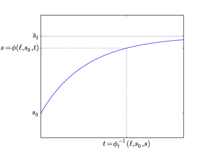
(a) $t\mapsto\phi(\ell,s_{0},t)$

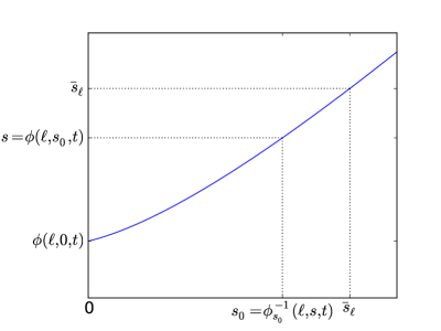
(b) $s_{0}\mapsto\phi(\ell,s_{0},t)$

Figure 1: Graphical representation of $t\mapsto\phi(\ell,s_{0},t)$ and $s_{0}\mapsto\phi(\ell,s_{0},t)$.

3.3 Bounds on the hitting times of the process

In this section, we will develop some irreducibility properties of the Crump-Young process through bounds on its hitting times, which will be useful to prove the mass ratio inequality in Section 3.4.3. To that end, let $K$ be a non empty compact set of $\mathbb{N}^{*}\times(0,\widebar{s}_{1})$ and let $s_{K}=\min_{(x,s)\in K}s$ and $S_{K}=\max_{(x,s)\in K}s$. We will prove that each point of $K\backslash\bigcup_{\ell\geq 1}(\ell,\widebar{s}_{\ell})$ can be reached, in a uniform way, from any point of $K$. Points $(\ell,\widebar{s}_{\ell})$ can not be reached.

There exists $L_{s_{K}}\in\mathbb{N}^{*}$, such that $\widebar{s}_{\ell}<s_{K}$ for all $\ell\geq L_{s_{K}}$ (see Lemma A.2), let then set ${L_{K}}=\max\{\max_{(\ell,s)\in K}\ell,\,L_{s_{K}}\}$. The constants $s_{K}$, $S_{K}$ and ${L_{K}}$ satisfy $K\subset\llbracket 1,{L_{K}}\rrbracket\times[s_{K},S_{K}]\subset\llbracket 1,{L_{K}}\rrbracket\times(\widebar{s}_{{L_{K}}},\widebar{s}_{1})$.

Let also

$$t_{\min}:=\max\left\{\phi_{\textsf{t}}^{-1}\left(1,\widebar{s}_{{L_{K}}},S_{K}\right),\,\,\phi_{\textsf{t}}^{-1}\left({L_{K}},\widebar{s}_{1},s_{K}\right)\right\}$$ (18)

be the maximum between the time to go from $\widebar{s}_{{L_{K}}}$ to $S_{K}$ with one individual and the time to go from $\widebar{s}_{1}$ to $s_{K}$ with ${L_{K}}$ individuals. As both times are finite then $t_{\min}<\infty$. Note that, from the monotony properties of the flow (see Lemma A.3) for all $s_{1},s_{2}$ such that $\widebar{s}_{{L_{K}}}\leq s_{1}\leq s_{2}\leq S_{K}$, then $\phi_{\textsf{t}}^{-1}(1,s_{1},s_{2})\leq\phi_{\textsf{t}}^{-1}\left(1,\widebar{s}_{{L_{K}}},S_{K}\right)\leq t_{\min}$ and for all $s_{1},s_{2}$ such that $s_{K}\leq s_{2}\leq s_{1}\leq\widebar{s}_{1}$, $\phi_{\textsf{t}}^{-1}({L_{K}},s_{1},s_{2})\leq\phi_{\textsf{t}}^{-1}\left({L_{K}},\widebar{s}_{1},s_{K}\right)\leq t_{\min}$. Then $t_{\min}$ is the minimal quantity such that, for all $s_{1},s_{2}$ satisfying $\widebar{s}_{{L_{K}}}\leq s_{1}\leq s_{2}\leq S_{K}$ or $s_{K}\leq s_{2}\leq s_{1}\leq\widebar{s}_{1}$, there exists $L\in\llbracket 1,{L_{K}}\rrbracket$, such that $\phi_{\textsf{t}}^{-1}(L,s_{1},s_{2})\leq t_{\min}$ (i.e. the substrate concentration $s_{2}$ is reachable from $s_{1}$ in a time less than $t_{\min}$ with a constant bacterial population in $\llbracket 1,{L_{K}}\rrbracket$).

Proposition 3.1.

For all $\tau_{0}>t_{\min}$, $\tau>\tau_{0}$, $\varepsilon>0$ and $\delta>0$, there exists $C>0$, such that, for all $(x,s)\in K$, for all $(y,r)\in K$ satisfying $|r-\widebar{s}_{y}|>\delta$, we have

$$\mathbb{P}_{(x,s)}(\tau-\varepsilon\leq\widetilde{T}_{y,r}\leq\tau)\geq C>0\,,$$

where $\widetilde{T}_{y,r}:=\inf\{t\geq\tau_{0},\,(X_{t},S_{t})=(y,r)\}$ is the first hitting time of $(y,r)$ after $\tau_{0}$.

Proof of Proposition 3.1 relies on sharp decomposition of all possibilities of combination of initial conditions. Instead of giving all details on the proof, we will expose its main steps and the technicalities are postponed in Appendix.

Proof.

Let

$$\widebar{\varepsilon}:=\min\left\{\frac{3\,\min\{s_{K}-\widebar{s}_{{L_{K}}},\,\widebar{s}_{1}-S_{K}\}}{\max\{D\,{\mathbf{s}}_{\textrm{\tiny\rm in}},\,k\,\mu(\widebar{s}_{1})\,{L_{K}}\}}\,,\,\frac{4\,\min\{s_{K}-\widebar{s}_{{L_{K}}},\,\widebar{s}_{1}-S_{K}\}\,D\,(\tau_{0}-t_{\min})/2}{\max\{D\,{\mathbf{s}}_{\textrm{\tiny\rm in}},\,k\,\mu(\widebar{s}_{1})\,{L_{K}}\}\,(1+D\,(\tau_{0}-t_{\min})/2)}\right\}.$$

We assume, without loss of generality, that $0<\varepsilon\leq\min\{\tau-\tau_{0};\widebar{\varepsilon}\}$ because if the result holds for all $\varepsilon>0$ sufficiently small, then it holds for all $\varepsilon>0$. Assuming $0<\varepsilon\leq\frac{3\,\min\{s_{K}-\widebar{s}_{{L_{K}}},\,\widebar{s}_{1}-S_{K}\}}{\max\{D\,{\mathbf{s}}_{\textrm{\tiny\rm in}},\,k\,\mu(\widebar{s}_{1})\,{L_{K}}\}}$ ensures that, for $(y,r)\in K$, $\widebar{s}_{{L_{K}}}\leq\phi_{\textsf{s}_{0}}^{-1}(y,r,\frac{\varepsilon}{3})\leq\widebar{s}_{1}$ (and consequently that $\widebar{s}_{{L_{K}}}\leq\phi_{\textsf{s}_{0}}^{-1}(y,r,\frac{\varepsilon}{4})\leq\widebar{s}_{1}$); see Lemma A.7-1 and Remark A.8. Consequently $\mathcal{S}_{y,r}^{\varepsilon}:=\llbracket 1,{L_{K}}\rrbracket\times\left[\phi_{\textsf{s}_{0}}^{-1}(y,r,\frac{\varepsilon}{3}),\phi_{\textsf{s}_{0}}^{-1}(y,r,\frac{\varepsilon}{4})\right]\subset\llbracket 1,{L_{K}}\rrbracket\times[\widebar{s}_{{L_{K}}},\widebar{s}_{1}]$.

To prove Proposition 3.1, we will prove that, with positive probability, the process:

1. reaches the set $\mathcal{S}_{y,r}^{\varepsilon}$ before $\tau_{0}$;

2. stays in this set until the time $\tau-\varepsilon$;

3. reaches $(y,r)$ in the time interval $[\tau-\varepsilon,\,\tau]$.

These steps are illustrated in Figure 2 and the associated probabilities are bounded from below in lemmas below. These ones are proved in Appendix B. To state them, let us introduce $\mathcal{E}_{y,r}^{\varepsilon}$, defined by

$$\mathcal{E}_{y,r}^{\varepsilon}:=\{(\ell,r^{\varepsilon}_{y,r})\,|\,\ell\in\llbracket 1,{L_{K}}\rrbracket\text{ and }\widebar{s}_{\ell}\geq r^{\varepsilon}_{y,r}\}\mathbin{\scalebox{1.5}{$\cup$}}\{(\ell,R^{\varepsilon}_{y,r})\,|\,\ell\in\llbracket 1,{L_{K}}\rrbracket\text{ and }\widebar{s}_{\ell}\leq R^{\varepsilon}_{y,r}\}\subset\mathcal{S}_{y,r}^{\varepsilon},$$

where $r^{\varepsilon}_{y,r}=\min(\phi_{\textsf{s}_{0}}^{-1}(y,r,\frac{\varepsilon}{3}),\phi_{\textsf{s}_{0}}^{-1}(y,r,\frac{\varepsilon}{4}))$ and $R^{\varepsilon}_{y,r}=\max(\phi_{\textsf{s}_{0}}^{-1}(y,r,\frac{\varepsilon}{3}),\phi_{\textsf{s}_{0}}^{-1}(y,r,\frac{\varepsilon}{4}))$. The set $\mathcal{E}_{y,r}^{\varepsilon}$ represents the points $(\ell,s)\in\mathcal{S}_{y,r}^{\varepsilon}$ such that $s$ belongs to the bounds of the substrate part $\left[\phi_{\textsf{s}_{0}}^{-1}(y,r,\frac{\varepsilon}{3}),\phi_{\textsf{s}_{0}}^{-1}(y,r,\frac{\varepsilon}{4})\right]$ and $\ell$ is such that the flow $t\mapsto\phi(\ell,s,t)$ leads the dynamics to stay in $\left[\phi_{\textsf{s}_{0}}^{-1}(y,r,\frac{\varepsilon}{3}),\phi_{\textsf{s}_{0}}^{-1}(y,r,\frac{\varepsilon}{4})\right]$, at least for small $t$, if $\phi_{\textsf{s}_{0}}^{-1}(y,r,\frac{\varepsilon}{3})\neq\phi_{\textsf{s}_{0}}^{-1}(y,r,\frac{\varepsilon}{4})$ (that is if $r\neq\widebar{s}_{y}$). Note that $\mathcal{E}_{y,r}^{\varepsilon}$ is well defined if $r=\widebar{s}_{y}$ and we obtain $\mathcal{E}_{y,\widebar{s}_{y}}^{\varepsilon}=\llbracket 1,{L_{K}}\rrbracket\times\{\widebar{s}_{y}\}$.

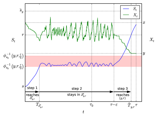
Figure 2: Example of dynamics of the process $(X_{t},S_{t})_{t}$ from $(x,s)$ to $(y,r)$, illustrating the three steps of the proof of Proposition 3.1. Step 1: the process reaches the set $\mathcal{S}_{y,r}^{\varepsilon}$ before $\tau_{0}$. Step 2: the process stays in $\mathcal{S}_{y,r}^{\varepsilon}$ until $\tau-\varepsilon$. Step 3: the process reaches $(y,r)$ before $\tau$.

Lemma 3.2.

For all $\tau_{0}>t_{\min}$, there exists $C_{1}^{\tau_{0}}>0$, such that, for all $(x,s)\in K$, for all $(y,r)\in K$ and for $0<\varepsilon\leq\frac{4\,\min\{\widebar{s}_{1}-S_{K},\,s_{K}-\widebar{s}_{{L_{K}}}\}\,D\,(\tau_{0}-t_{\min})/2}{\max\{D\,{\mathbf{s}}_{\textrm{\tiny\rm in}},\,k\,\mu(\widebar{s}_{1})\,{L_{K}}\}\,(1+D\,(\tau_{0}-t_{\min})/2)}$,

$$\mathbb{P}_{(x,s)}\big{(}T_{\mathcal{E}_{y,r}^{\varepsilon}}\leq\tau_{0}\big{)}\geq C_{1}^{\tau_{0}},$$

where $T_{\mathcal{E}_{y,r}^{\varepsilon}}:=\inf\left\{t\geq 0,\,(X_{t},S_{t})\in\mathcal{E}_{y,r}^{\varepsilon}\right\}$.

Lemma 3.3.

Let $0<\varepsilon\leq\frac{3\,\min\{s_{K}-\widebar{s}_{{L_{K}}},\,\widebar{s}_{1}-S_{K}\}}{\max\{D\,{\mathbf{s}}_{\textrm{\tiny\rm in}},\,k\,\mu(\widebar{s}_{1})\,{L_{K}}\}}$, $\delta>0$ and $T>0$. Then there exists $C^{\varepsilon,\delta,T}_{2}>0$, such that, for all $(y,r)\in K$ satisfying $|r-\widebar{s}_{y}|>\delta$, for all $(x,s)\in\mathcal{E}_{y,r}^{\varepsilon}$,

$$\mathbb{P}_{(x,s)}\left((X_{t},S_{t})\in\mathcal{S}_{y,r}^{\varepsilon},\,\forall t\in[0,T]\right)\geq C^{\varepsilon,\delta,T}_{2}\,.$$

Lemma 3.4.

Let $0<\varepsilon\leq\frac{3\,\min\{s_{K}-\widebar{s}_{{L_{K}}},\,\widebar{s}_{1}-S_{K}\}}{\max\{D\,{\mathbf{s}}_{\textrm{\tiny\rm in}},\,k\,\mu(\widebar{s}_{1})\,{L_{K}}\}}$ and $\delta>0$. Then there exists $C^{\varepsilon,\delta}_{3}>0$, such that, for all $(y,r)\in K$ satisfying $|r-\widebar{s}_{y}|>\delta$, for all $(x,s)\in\mathcal{S}_{y,r}^{\varepsilon}$,

$$\mathbb{P}_{(x,s)}\Big{(}T_{y,r}\leq\varepsilon\Big{)}\geq C^{\varepsilon,\delta}_{3}$$

with $T_{y,r}:=\inf\{t\geq 0,\,(X_{t},S_{t})=(y,r)\}$ the first hitting time of $(y,r)$.

Even not optimal, some explicit expressions of $C_{1}^{\tau_{0}}$, $C^{\varepsilon,\delta,T}_{2}$, $C^{\varepsilon,\delta}_{3}$ of the previous lemmas are given in Appendix B. Let us show below that they imply the conclusion of Proposition 3.1.

$$\mathbb{P}_{(x,s)}(\tau-\varepsilon\leq\widetilde{T}_{y,r}\leq\tau)$$

$$\qquad\qquad\geq\mathbb{P}_{(x,s)}\Big{(}\{T_{\mathcal{E}_{y,r}^{\varepsilon}}\leq\tau_{0}\}\cap\big{\{}(X_{t},S_{t})\in\mathcal{S}_{y,r}^{\varepsilon},\,\forall t\in[T_{\mathcal{E}_{y,r}^{\varepsilon}},\,\tau-\varepsilon]\big{\}}$$

$$\qquad\qquad\qquad\qquad\qquad\qquad\cap\{\tau-\varepsilon\leq\widetilde{T}_{y,r}\leq\tau\}\Big{)}$$

$$\qquad\qquad\geq\mathbb{P}_{(x,s)}\big{(}T_{\mathcal{E}_{y,r}^{\varepsilon}}\leq\tau_{0}\big{)}\,$$

$$\qquad\qquad\quad\times\mathbb{P}_{(x,s)}\Big{(}(X_{t},S_{t})\in\mathcal{S}_{y,r}^{\varepsilon},\,\forall t\in[T_{\mathcal{E}_{y,r}^{\varepsilon}},\,\tau-\varepsilon]\ |\ T_{\mathcal{E}_{y,r}^{\varepsilon}}\leq\tau_{0}\Big{)}$$

$$\qquad\qquad\quad\times\mathbb{P}_{(x,s)}\Big{(}\tau-\varepsilon\leq\widetilde{T}_{y,r}\leq\tau\ |\ T_{\mathcal{E}_{y,r}^{\varepsilon}}\leq\tau_{0},\,(X_{t},S_{t})\in\mathcal{S}_{y,r}^{\varepsilon},\,\forall t\in[T_{\mathcal{E}_{y,r}^{\varepsilon}},\,\tau-\varepsilon]\Big{)}\,.$$ (19)

By Lemma  3.2, the first probability of the last member of (19) is bounded from below by a constant $C_{1}^{\tau_{0}}>0$. By Lemma 3.3 and the Markov property the second probability is bounded from below by a constant $C^{\varepsilon,\delta,\tau}_{2}>0$. By definition, $\widetilde{T}_{y,r}\geq\tau_{0}$, moreover $(y,r)\notin\mathcal{S}_{y,r}^{\varepsilon}$, therefore on the event ${\{(X_{0},S_{0})=(x,s),\,T_{\mathcal{E}_{y,r}^{\varepsilon}}\leq\tau_{0},\,(X_{t},S_{t})\in\mathcal{S}_{y,r}^{\varepsilon},\,\forall t\in[T_{\mathcal{E}_{y,r}^{\varepsilon}},\,\tau-\varepsilon]\}}$ we have $\widetilde{T}_{y,r}\geq\tau-\varepsilon$ almost surely. By Lemma 3.4 and Markov property, the third probability is bounded from below by a constant $C^{\varepsilon,\delta}_{3}>0$, which achieves the proof. ∎

3.4 Proof of the sufficient conditions leading to Theorem 2.2

We prove in this section that the three conditions – Bounds on Lyapunov functions (BLF1) and (BLF2); Small set assertion (SSA) and Mass ratio inequality (MRI) – hold. As it was proved in Section 3.1 that they imply Theorem 2.2, it will conclude the proof of this theorem.

Bounds on Lyapunov functions (BLF1) and (BLF2) are given by Lemma 3.6; Small set assertion (SSA) is given by Lemma 3.8; Mass ratio inequality(MRI) is given by Lemma 3.9.

3.4.1 Bounds on Lyapunov functions

Let $\widetilde{V}(x,s)=V(x,s)\,\mathbf{1}_{(x,s)\in\mathbb{N}^{*}\times(0,\widebar{s}_{1})}$ for all $(x,s)\in(\mathbb{N}^{*}\times(0,\widebar{s}_{1}))\cup(\{0\}\times(0,{\mathbf{s}}_{\textrm{\tiny\rm in}}))$, where we recall that $V$ is defined on $\mathbb{N}^{*}\times(0,\widebar{s}_{1})$ by (11). Assumptions (10) and a simple computation lead to the following lemma, whose the proof is postponed in Appendix (see Section B.5).

Lemma 3.5.

There exists $\eta>D$ and $\zeta>0$ such that

$$\mathcal{L}\widetilde{V}\leq-\eta\widetilde{V}+\zeta\psi,$$

on $(\mathbb{N}^{*}\times(0,\widebar{s}_{1}))\cup(\{0\}\times(0,{\mathbf{s}}_{\textrm{\tiny\rm in}}))$, where $\mathcal{L}$ is the infinitesimal generator of $(X_{t},S_{t})_{t\geq 0}$ defined by (2).

Using well known martingale properties associated to Crump-Young model, the drift condition exposed in Lemma 3.5 before extends to the following lemma.

Lemma 3.6.

There exists $\eta>D$ and $\zeta>0$, such that for all $t\geq 0$, $x\in\mathbb{N}^{*}$ and $s\in(0,\widebar{s}_{1})$, we have

$$e^{-Dt}\,x=e^{-Dt}\psi(x,s)\leq\mathbb{E}_{(x,s)}[\psi(X_{t},S_{t})]\leq e^{(\mu(\widebar{s}_{1})-D)t}\,\psi(x,s)=e^{(\mu(\widebar{s}_{1})-D)t}\,x$$ (20)

and

$$\mathbb{E}_{(x,s)}\left[V(X_{t},S_{t})\,\mathbf{1}_{X_{t}\neq 0}\right]\leq e^{-\eta t}V(x,s)+\zeta\frac{e^{(\mu(\widebar{s}_{1})-D)t}}{\eta-D}\psi(x,s)\,.$$ (21)

Proof.

It is classical (see for example Section 4 of [9]) that, for $f\in\mathcal{C}^{0,1}(\mathbb{N}\times\mathbb{R}_{+})$, the process

$$\left(f(X_{t},S_{t})-f(X_{0},S_{0})-\int_{0}^{t}\mathcal{L}f(X_{u},S_{u})\mathrm{d}u\right)_{t\geq 0}$$ (22)

is a local martingale. As $\psi\leq\widetilde{V}$ on $(\mathbb{N}^{*}\times(0,\widebar{s}_{1}))\cup(\{0\}\times(0,{\mathbf{s}}_{\textrm{\tiny\rm in}}))$, from Lemma 3.5, $\widetilde{V}$ satisfies $\mathcal{L}\widetilde{V}\leq\zeta\widetilde{V}$ for some $\zeta>0$. Then using classical stopping time arguments (see [1, Section 6.2.] or [28, Theorem 2.1] and its proof for instance), we can show that it is a martingale when $f=\widetilde{V}$ and then that $(\mathbb{E}_{(x,s)}[\widetilde{V}(X_{t},S_{t})])_{t\in[0,T]}$ is bounded for all $T>0$. Consequently, (22) is also a martingale for $f=\psi$, because $\psi\leq\widetilde{V}$. Then, from the dominated convergence theorem and the fact that, from the expression of $\psi$,

$$-D\psi\leq\mathcal{L}\psi\leq(\mu(\widebar{s}_{1})-D)\psi,$$

we obtain (20). Similarly, by the linearity of $\mathcal{L}$, from Lemma 3.5 and (20),

$$\mathcal{L}\left(\widetilde{V}-\frac{\zeta}{\eta-D}\psi\right)\leq-\eta\widetilde{V}+\zeta\psi+\frac{\zeta}{\eta-D}D\psi=-\eta\left(\widetilde{V}-\frac{\zeta}{\eta-D}\psi\right)$$

then, for all $(x,s)\in\mathbb{N}^{*}\times(0,\widebar{s}_{1})$

$$\mathbb{E}_{(x,s)}\left[V(X_{t},S_{t})\,\mathbf{1}_{X_{t}\neq 0}\right] =\mathbb{E}_{(x,s)}\left[\widetilde{V}(X_{t},S_{t})\right]$$

$$\leq e^{-\eta\,t}\widetilde{V}(x,s)+\frac{\zeta}{\eta-D}\left(\mathbb{E}_{(x,s)}\left[\psi(X_{t},S_{t})\right]-e^{-\eta\,t}\psi(x,s)\right)$$

$$\leq e^{-\eta\,t}V(x,s)+\frac{\zeta}{\eta-D}\,e^{(\mu(\widebar{s}_{1})-D)t}\psi(x,s)\,.$$

and (21) holds. ∎

Let us point out some similarities between our approach and the proof of [14, Theorem 4.1]. Indeed, to prove existence of the QSD, tightness is enough and is garanted by the use of Lyapunov functions (see for instance [13, Theorem 4.2]). However, the interest of our work is to go behind the existence of the QSD by proving uniqueness and convergence through sharp estimate on hitting times and new Harris Theorem.

3.4.2 Small set assertion

Let $K$ be a compact set of $\mathbb{N}^{*}\times(0,\widebar{s}_{1})$. Consistently with notation of Section 3.3, let $s_{K}:=\min_{(x,s)\in K}s$ and $S_{K}:=\min_{(x,s)\in K}s$ be respectively the minimal and maximal substrate concentration of elements of $K$.

Our aim in this subsection is to prove the small set assertion (SSA) established page SSA by introducing the coupling measure $\nu$. The proof is based on Lemma 3.7 below.

Lemma 3.7.

Let $\tau>0$, let $0<s_{0}<s_{K}$, $s_{1}>s_{0}$ and $x\in\mathbb{N}^{*}$. Then there exists $\epsilon_{0}>0$ such that, for all $(y,r)\in K$,

$$\mathbb{P}_{(y,r)}\left((X_{\tau},S_{\tau})\in\{x\}\times[s_{0},s_{1}]\right)\geq\epsilon_{0}\,.$$

Lemma 3.7 is proved in Appendix (see Section B.6). As Proposition 3.1, its proof relies on a sharp study of the paths. From this, we deduce the next result which is one the cornerstone of the proof of Theorem 2.2.

Lemma 3.8.

For every $\tau>0$, there exists $\epsilon>0$ and a probability measure $\nu$ on $\mathbb{N^{*}}\times(0,\widebar{s}_{1})$ such that

$$\forall(y,r)\in K,\quad\mathbb{P}_{(y,r)}\left((X_{\tau},S_{\tau})\in\cdot\right)\geq\epsilon\nu.$$ (23)

If moreover $K=\llbracket 1,N\rrbracket\times[\delta_{1},\delta_{2}]$, for some $N\in\mathbb{N}^{*}$ and $\delta_{2}>\delta_{1}>0$, then we can choose $\nu$ such that $\nu(K)=1$.

Proof.

Starting from $(y,r)\in K$, the discrete component can reach any point $z$ of $\mathbb{N}^{*}$ in any time interval with positive probability, so we can easily use any Dirac mass $\delta_{z}$ (times a constant) as a lower bound for the first marginal of the law of $(X_{\tau},S_{\tau})$. Let us use $z=1$. For the continuous component, we can use the randomness of the last jump time to prove that its law has a lower bound with Lebesgue density. Consequently to prove (23), we consider the paths going to $\{2\}\times[s_{0},s_{1}]$ for some $s_{1}\geq s_{0}$ well chosen, then being subjected to a washout, and we study the last jump to construct a lower bound with density.

Let us consider some $\widebar{s}_{1}>s_{1}>s_{0}>0$ such that $s_{0}<s_{K}$ and $0<\tau_{0}<\tau$ which will be fixed at the end of the proof. On the one hand, from Lemma 3.7, there exists $\epsilon_{0}>0$ such that for all $(y,r)\in K$,

$$\mathbb{P}_{(y,r)}\left((X_{\tau-\tau_{0}},S_{\tau-\tau_{0}})\in\{2\}\times[s_{0},s_{1}]\right)\geq\epsilon_{0}.$$ (24)

On the other hand, let $f$ be any positive function, $s\in[s_{0},s_{1}]$ and $t>0$. By conditioning on the first jump time and using the Markov property, we have

$$\mathbb{E}_{(2,s)}\left[f(X_{t},S_{t})\right] =e^{-2\,D\,t-2\,\int_{0}^{t}\mu(\phi(2,s,u))\mathrm{d}u}\,f\left(2,\phi(2,s,t)\right)$$

$$+\int_{0}^{t}2\,D\,e^{-2\,D\,v-2\,\int_{0}^{v}\mu(\phi(2,s,u))\mathrm{d}u}\,\mathbb{E}_{(1,\phi(2,s,v))}\left[f(X_{t-v},S_{t-v})\right]\mathrm{d}v$$

$$+\int_{0}^{t}2\,\mu(\phi(2,s,v))\,e^{-2\,D\,v-2\,\int_{0}^{v}\mu(\phi(2,s,u))\mathrm{d}u}\,\mathbb{E}_{(3,\phi(2,s,v))}\left[f(X_{t-v},S_{t-v})\right]\mathrm{d}v$$

$$\geq\int_{0}^{t}2\,D\,e^{-2\,D\,v-2\,\int_{0}^{v}\mu(\phi(2,s,u))\mathrm{d}u}\times e^{-\,(t-v)\,D-\int_{0}^{t-v}\mu(\phi(1,\phi(2,s,v),u))\mathrm{d}u}$$

$$\qquad\qquad\times f\left(1,\phi(1,\phi(2,s,v),t-v)\right)\mathrm{d}v,$$

where the last bound comes from a second use of the Markov property on the second term. Roughly, we bounded our expectation by considering the event “the first event is a washout and occurs during the time interval $(0,t)$ and no more jump occurs until $t$”.

As $s\mapsto\phi(x,s,u)$ and $x\mapsto\phi(x,s,u)$ are respectively increasing and decreasing (see Lemma A.1) and $\mu$ is increasing, we have for all $s\in[s_{0},s_{1}]$

$$\mu(\phi(2,s,u))\leq\mu(\phi(1,s_{1},u)),$$

hence

$$\mathbb{E}_{(2,s)}\left[f(X_{t},S_{t})\right] \geq 2\,D\,e^{-2\,D\,t}e^{-2\,\int_{0}^{t}\mu(\phi(1,s_{1},u))\mathrm{d}u}\,\int_{0}^{t}f\left(1,\phi(1,\phi(2,s,v),t-v)\right)\mathrm{d}v.$$

By the flow property and Lemma A.1, for $0<\varepsilon<t-v$, we have

$$\phi(1,\phi(2,s,v),t-v) =\phi(1,\phi(1,\phi(2,s,v),\varepsilon),t-(v+\varepsilon))$$

$$>\phi(1,\phi(2,\phi(2,s,v),\varepsilon),t-(v+\varepsilon))$$

$$=\phi(1,\phi(2,s,v+\varepsilon),t-(v+\varepsilon))$$

and then $v\mapsto\phi(1,\phi(2,s,v),t-v)$ is strictly decreasing on $[0,t]$. Moreover from (16) the derivative of $u\mapsto\phi(1,s,u)$ is bounded from above by $D\,{\mathbf{s}}_{\textrm{\tiny\rm in}}$. As $r\mapsto\phi(1,r,t-v)$ is increasing for $r\leq\widebar{s}_{1}$ from Lemma A.3, then from the expression $\phi(1,r,t-v)=r+\int_{0}^{t-v}(D({\mathbf{s}}_{\textrm{\tiny\rm in}}-\phi(1,r,u))-k\,\mu(\phi(1,r,u)))\,\mathrm{d}u$, we have $0\leq\frac{\mathrm{d}}{\mathrm{d}r}\phi(1,r,t-v)\leq 1$. In addition, either $s\leq\widebar{s}_{2}$ and $\frac{\mathrm{d}}{\mathrm{d}v}\phi(2,s,v)\geq 0$ or $s<\widebar{s}_{2}$ and from (16) and Lemma A.3, $\frac{\mathrm{d}}{\mathrm{d}v}\phi(2,s,v)\geq-2\,k\,\mu(\widebar{s}_{2})$. So finally, from the chain rule formula

$$\frac{\mathrm{d}}{\mathrm{d}v}\phi(1,\phi(2,s,v),t-v) =\frac{\mathrm{d}}{\mathrm{d}v}\phi(2,s,v)\,\frac{\mathrm{d}}{\mathrm{d}r}\phi(1,r,t-v)_{|_{r=\phi(2,s,v)}}-\frac{\mathrm{d}}{\mathrm{d}u}\phi(1,\phi(2,s,v),u)_{|_{u=t-v}},$$

the derivative of $v\mapsto\phi(1,\phi(2,s,v),t-v)$ is then bounded from below by $-D\,{\mathbf{s}}_{\textrm{\tiny\rm in}}-2\,k\,\mu(\widebar{s}_{2})$. By a change of variable, for every $s_{0}<s_{1}$, we have for $c_{0}=\left[D\,{\mathbf{s}}_{\textrm{\tiny\rm in}}+2\,k\,\mu(\widebar{s}_{2})\right]^{-1}$ and for $s\in(s_{0},s_{1})$

$$\mathbb{E}_{(2,s)}\left[f(X_{t},S_{t})\right] \geq c_{0}\,2\,D\,e^{-2\,D\,t}e^{-2\,\int_{0}^{t}\mu(\phi(1,s_{1},u))\mathrm{d}u}\,\int_{\phi(2,s,t)}^{\phi(1,s,t)}f(1,w)\mathrm{d}w$$

$$\geq c_{0}\,2\,De^{-2\,D\,t}\,e^{-2\,\int_{0}^{t}\mu(\phi(1,s_{1},u))\mathrm{d}u}\,\int_{\phi(2,s_{1},t)}^{\phi(1,s_{0},t)}f(1,w)\mathrm{d}w,$$

where the last term is non negative as soon as $\phi(2,s_{1},t)<\phi(1,s_{0},t)$. First, we fix any $s_{0}<s_{K}$. As $\phi(2,s_{0},t)<\phi(1,s_{0},t)$, by continuity, we can find $s_{1}>s_{0}$ satisfying $\phi(2,s_{1},t)<\phi(1,s_{0},t)$. Fixing such two points $s_{0}$ and $s_{1}$ for $t=\tau_{0}$ with $0<\tau_{0}<\tau$, then leads to

$$\forall s\in[s_{0},s_{1}],\quad\mathbb{P}_{(2,s)}\left((X_{\tau_{0}},S_{\tau_{0}})\in\cdot\right)\geq\epsilon_{1}\nu,$$ (25)

with

$$\nu(dy,ds)=\delta_{1}(dy)\frac{\mathbf{1}_{[\phi(2,s_{1},\tau_{0}),\phi(1,s_{0},\tau_{0})]}(s)}{\phi(1,s_{0},\tau_{0})-\phi(2,s_{1},\tau_{0})}ds,$$

and

$$\epsilon_{1}=c_{0}\,2\,D\,e^{-2\,D\,\tau_{0}}\,e^{-2\,\int_{0}^{\tau_{0}}\mu(\phi(1,s_{1},u))\mathrm{d}u}(\phi(1,s_{0},\tau_{0})-\phi(2,s_{1},\tau_{0})).$$

As a consequence, from (24) and (25), Equation (23) holds with $\epsilon=\epsilon_{0}\epsilon_{1}$, by Markov property.

If $K=\llbracket 1,N\rrbracket\times[\delta_{1},\delta_{2}]$, even if it means choosing $\tau_{0}$ small enough, $s_{0}$ and $s_{1}$ can be chosen such that they furthermore satisfy $\phi(1,s_{0},\tau_{0})>\delta_{1}$ and $\phi(2,s_{1},\tau_{0})<\delta_{2}$. Then $\nu(K)>0$ and (25) holds with $\widetilde{\epsilon}_{1}$ and the probability measure $\widetilde{\nu}$, satisfying $\widetilde{\nu}(K)=1$, defined by

$$\widetilde{\nu}=\frac{\nu\left(\mathbf{1}_{K}\,\cdot\right)}{\nu(K)},\qquad\widetilde{\epsilon}_{1}=\epsilon_{1}\,\nu(K)\,.$$

Note that if $\tau_{0}<\phi_{\textsf{t}}^{-1}(2,0,\delta_{2})$ (i.e. $\phi_{\textsf{s}_{0}}^{-1}(2,\delta_{2},\tau_{0})>0$) then such $s_{0}$ and $s_{1}$ exists. In fact, we can choose $s_{0}$ and $s_{1}$ such that $s_{0}\in(\phi_{\textsf{s}_{0}}^{-1}(1,\delta_{1},\tau_{0}),\delta_{1}\wedge\phi_{\textsf{s}_{0}}^{-1}(2,\delta_{2},\tau_{0}))$ and $s_{1}\in(s_{0},\phi_{\textsf{s}_{0}}^{-1}(2,\delta_{2},\tau_{0})\wedge\phi_{\textsf{s}_{0}}^{-1}(2,\phi(1,s_{0},\tau_{0}),\tau_{0}))$. As $\delta_{1}<\widebar{s}_{1}$ and as $\ell\mapsto\phi_{\textsf{s}_{0}}^{-1}(\ell,s,\tau_{0})$ and $s\mapsto\phi_{\textsf{s}_{0}}^{-1}(\ell,s,\tau_{0})$ are both increasing (by definition of $\phi_{\textsf{s}_{0}}^{-1}$ and by Lemma A.1), we can check that $\delta_{1}$ and $\delta_{2}$ are well defined. Moreover $s0$ and $s_{1}$ are such that $s_{0}<\delta_{1}=s_{K}$ and $s_{0}<s_{1}$, and by Lemma A.1, we have

$$\phi(1,s_{0},\tau_{0})>\phi(1,\phi_{\textsf{s}_{0}}^{-1}(1,\delta_{1},\tau_{0}),\tau_{0})\geq\delta_{1};$$

$$\phi(2,s_{1},\tau_{0})<\phi(2,\phi_{\textsf{s}_{0}}^{-1}(2,\delta_{2},\tau_{0}),\tau_{0})=\delta_{2};$$

$$\phi(2,s_{1},t)<\phi(2,\phi_{\textsf{s}_{0}}^{-1}(2,\phi(1,s_{0},\tau_{0}),\tau_{0}),\tau_{0})=\phi(1,s_{0},\tau_{0}).\qed$$

3.4.3 Mass ratio inequality

Our aim in this subsection is to prove the mass ratio inequality (MRI) given on page MRI by using our bounds on the hitting time given in Proposition 3.1.

Lemma 3.9.

Let $K$ be a compact set of $\mathbb{N}^{*}\times(0,\widebar{s}_{1})$, then

$$\sup_{(x,s),(y,r)\in K}\sup_{t\geq 0}\frac{\mathbb{E}_{(y,r)}\left[\psi(X_{t},S_{t})\right]}{\mathbb{E}_{(x,s)}\left[\psi(X_{t},S_{t})\right]}<+\infty.$$

Proof.

We set $L=\max_{(x,s)\in K}x$, $s_{K}=\min_{(\ell,s)\in K}s$ and $S_{K}=\max_{(\ell,s)\in K}s$. Let

$$0<\delta<\min\left\{\frac{1}{2}\min_{y,z\in K,\,y\neq z}|\widebar{s}_{y}-\widebar{s}_{z}|\,;\,\widebar{s}_{1}-S_{K}\right\}.$$ (26)

Note that, from Lemma A.2, elements of $(\widebar{s}_{\ell})_{\ell\in K}$ are all distinct and then the right member of (26) is then strictly positive. Let also $\widetilde{K}:=\llbracket 1,L+1\rrbracket\times[\min\{s_{K},\widebar{s}_{L}\},\max\{S_{K},\widebar{s}_{2}\}]$ be a compact set of $\mathbb{N}^{*}\times(0,\widebar{s}_{1})$ such that $K\subset\widetilde{K}$ and let $t_{\min}$ defined by (18) for the compact set $\widetilde{K}$. Let $\tau>t_{\min}$, from (20),

$$\sup_{(x,s),(y,r)\in K}\sup_{t\leq\tau}\frac{\mathbb{E}_{(y,r)}\left[\psi(X_{t},S_{t})\right]}{\mathbb{E}_{(x,s)}\left[\psi(X_{t},S_{t})\right]}\leq e^{\mu(\widebar{s}_{1})\,\tau}\,L<+\infty,$$

then it remains to prove that there exist $C>0$, such that for all $(x,s),(y,r)\in K$ and $t\geq\tau$, we have

$$\mathbb{E}_{(y,r)}\left[\psi(X_{t},S_{t})\right]\leq C\,\mathbb{E}_{(x,s)}\left[\psi(X_{t},S_{t})\right].$$ (27)

We first show by Proposition 3.1 that (27) holds for $(y,r)\in\widetilde{K}\setminus\left(\bigcup_{\ell=1}^{L+1}\{\ell\}\times\mathcal{B}(\widebar{s}_{\ell},\delta)\right)$ with $\mathcal{B}(\widebar{s}_{\ell},\delta):=\{r,\,|r-\widebar{s}_{\ell}|\leq\delta\}$. Then for $(y,r)\in K\cap\bigcup_{\ell=1}^{L}\{\ell\}\times\mathcal{B}(\widebar{s}_{\ell},\delta)$, conditioning on the first event, either no jump occurs and we make use of (20), or a jump occurs and the process after the jump belongs to $\widetilde{K}\setminus\left(\bigcup_{\ell=1}^{L+1}\{\ell\}\times\mathcal{B}(\widebar{s}_{\ell},\delta)\right)$ which then allows to use (27).

By the Markov property, for all $0\leq u\leq t$, for all $(y,r)\in\widetilde{K}$, $\mathbb{E}_{(y,r)}\left[\psi(X_{t},S_{t})\right]=\mathbb{E}_{(y,r)}\left[\mathbb{E}_{(X_{t-u},S_{t-u})}\left[\psi(X_{u},S_{u})\right]\right]$. Applying (20) to $\mathbb{E}_{(X_{t-u},S_{t-u})}\left[\psi(X_{u},S_{u})\right]$, we then obtain

$$e^{-D\,u}\,\mathbb{E}_{(y,r)}\left[\psi(X_{t-u},S_{t-u})\right]\leq\mathbb{E}_{(y,r)}\left[\psi(X_{t},S_{t})\right]\leq e^{(\mu(\widebar{s}_{1})-D)u}\,\mathbb{E}_{(y,r)}\left[\psi(X_{t-u},S_{t-u})\right].$$ (28)

Mimicking the arguments of [11, Theorem 1.1], we then deduce that for every $(x,s)\in K\subset\widetilde{K}$ and $(y,r)\in\widetilde{K}\setminus\left(\bigcup_{\ell=1}^{L+1}\{\ell\}\times\mathcal{B}(\widebar{s}_{\ell},\delta)\right)$, for all $t\geq\tau$,

$$\mathbb{E}_{(x,s)}\left[\psi(X_{t},S_{t})\right] \geq\mathbb{E}_{(x,s)}\left[\mathbf{1}_{T_{y,r}\leq\tau}\times\mathbb{E}_{(y,r)}\left[\psi\left(X_{t-u},S_{t-u}\right)\right]_{|_{u=T_{y,r}}}\right]$$

$$\geq\mathbb{P}_{(x,s)}\left(T_{y,r}\leq\tau\right)\int_{0}^{\tau}\mathbb{E}_{(y,r)}\left[\psi\left(X_{t-u},S_{t-u}\right)\right]\sigma^{x,s}_{y,r}(\mathrm{d}u)$$

$$\geq\widetilde{C}\int_{0}^{\tau}e^{-(\mu(\widebar{s}_{1})-D)u}\sigma^{x,s}_{y,r}(\mathrm{d}u)\mathbb{E}_{(y,r)}\left[\psi(X_{t},S_{t})\right]$$

$$\geq\widetilde{C}e^{-(\mu(\widebar{s}_{1})-D)\tau}\mathbb{E}_{(y,r)}\left[\psi(X_{t},S_{t})\right],$$ (29)

with $T_{y,r}:=\inf\{t\geq 0,\,(X_{t},S_{t})=(y,r)\}$ the first hitting time of $(y,r)$ and $\widetilde{C}>0$. In the first line, we used the strong Markov property, in the second line $\sigma^{x,s}_{y,r}$ represents the law of $T_{y,r}$ conditionally to $\{((X_{0},S_{0})=(x,s))\cap(T_{y,r}\leq\tau)\}$ and the third line comes from (28) and Proposition 3.1.

It remains to extend the previous inequality to $(y,r)\in K\cap\bigcup_{\ell=1}^{L}\{\ell\}\times\mathcal{B}(\widebar{s}_{\ell},\delta)$. By conditioning on the first jump and using Markov property, we have

$$\mathbb{E}_{(y,r)}\left[\psi(X_{t},S_{t})\right] =e^{-D\,y\,t-y\,\int_{0}^{t}\mu(\phi(y,r,u))\mathrm{d}u}\,\psi\left(y,\phi(y,r,t)\right)$$

$$+\int_{0}^{t}y\,D\,e^{-D\,y\,v-y\,\int_{0}^{v}\mu(\phi(y,r,u))\mathrm{d}u}\,\mathbb{E}_{(y-1,\phi(y,r,v))}\left[\psi(X_{t-v},S_{t-v})\right]\mathrm{d}v$$

$$+\int_{0}^{t}y\,\mu(\phi(y,r,v))e^{-D\,y\,v-y\,\int_{0}^{v}\mu(\phi(y,r,u))\mathrm{d}u}\,\mathbb{E}_{(y+1,\phi(y,r,v))}\left[\psi(X_{t-v},S_{t-v})\right]\mathrm{d}v.$$ (30)

First notice that, as $\delta<\widebar{s}_{1}-S_{K}$, then ($y,r)$ necessarily satisfies $y\geq 2$. Therefore $(y-1,\phi(y,r,v))\in\widetilde{K}$ and $(y+1,\phi(y,r,v))\in\widetilde{K}$ (see Lemma A.3).

From the definition of $\psi$ and (20), we have, for any $(x,s)\in K$

$$\psi\left(y,\phi(y,r,t)\right) =\frac{y}{x}\psi\left(x,s\right)\leq\frac{y}{x}\,e^{D\,t}\,\mathbb{E}_{(x,s)}\left[\psi(X_{t},S_{t})\right].$$ (31)

From (28),

$$\mathbb{E}_{(y-1,\phi(y,r,v))}\left[\psi(X_{t-v},S_{t-v})\right]\leq e^{D\,v}\,\mathbb{E}_{(y-1,\phi(y,r,v))}\left[\psi(X_{t},S_{t})\right].$$

Now as $(y,r)\in\bigcup_{\ell=1}^{L}\{\ell\}\times\mathcal{B}(\widebar{s}_{\ell},\delta)$, then $r\in\mathcal{B}(\widebar{s}_{y},\delta),$ and $\phi(y,r,v)\in\mathcal{B}(\widebar{s}_{y},\delta)$ for all $v\geq 0$ because of Lemma A.3 (i.e. equilibrium points are attractive). Thus, by definition of $\delta$, we have

$$\left|\phi(y,r,v)-\widebar{s}_{y-1}\right|\geq\left|\widebar{s}_{y-1}-\widebar{s}_{y}\right|-\left|\phi(y,r,v)-\widebar{s}_{y}\right|>2\delta-\delta=\delta,$$

then

$$(y-1,\phi(y,r,v))\notin\bigcup_{\ell=1}^{L}\{\ell\}\times\mathcal{B}(\widebar{s}_{\ell},\delta).$$

We can then apply (28) and (29) to obtain

$$\mathbb{E}_{(y-1,\phi(y,r,v))}\left[\psi(X_{t-v},S_{t-v})\right] \leq e^{D\,v}\,\mathbb{E}_{(y-1,\phi(y,r,v))}\left[\psi(X_{t},S_{t})\right]$$

$$\leq e^{D\,v}\,\widetilde{C}^{-1}e^{(\mu(\widebar{s}_{1})-D)\tau}\mathbb{E}_{(x,s)}\left[\psi(X_{t},S_{t})\right]\,.$$ (32)

Similarly, we have

$$\mathbb{E}_{(y+1,\phi(y,r,v))}\left[\psi(X_{t-v},S_{t-v})\right]\leq e^{D\,v}\,\widetilde{C}^{-1}e^{(\mu(\widebar{s}_{1})-D)\tau}\mathbb{E}_{(x,s)}\left[\psi(X_{t},S_{t})\right]\,.$$ (33)

From (30)-(31)-(32) and (33), we then obtain

$$\mathbb{E}_{(y,r)}\left[\psi(X_{t},S_{t})\right] \leq\mathbb{E}_{(x,s)}\left[\psi(X_{t},S_{t})\right]\,\Big{(}e^{-D\,(y-1)\,t-y\,\int_{0}^{t}\mu(\phi(y,r,u))\mathrm{d}u}\frac{y}{x}$$

$$\quad+\widetilde{C}^{-1}\,e^{(\mu(\widebar{s}_{1})-D)\tau}\,\int_{0}^{t}y\,(D+\mu(\phi(y,r,v)))\,e^{-D\,(y-1)\,v-y\,\int_{0}^{v}\mu(\phi(y,r,u))\mathrm{d}u}\,\mathrm{d}v\Big{)}\,.$$

$$\leq(L\wedge\widetilde{C}^{-1}e^{(\mu(\widebar{s}_{1})-D)\tau})\,\mathbb{E}_{(x,s)}\left[\psi(X_{t},S_{t})\right]$$

$$\qquad\times\Big{(}1+\,\int_{0}^{t}D\,e^{-D\,(y-1)\,v-y\,\int_{0}^{v}\mu(\phi(y,r,u))\mathrm{d}u}\,\mathrm{d}v\Big{)}\,.$$

As $y\geq 2$, then

$$\int_{0}^{t}D\,e^{-D\,(y-1)\,v-\int_{0}^{v}y\mu(\phi(y,r,u))\mathrm{d}u}\,\mathrm{d}v \leq\int_{0}^{t}D\,e^{-D\,v}\mathrm{d}v\leq 1$$

and (27) holds with $C:=2\,(L\wedge\widetilde{C}^{-1}e^{(\mu(\widebar{s}_{1})-D)\tau})$, which achieves the proof. ∎

4 Proof of Corollary 2.3

Let us now show that the convergence towards the quasi-stationary distribution $\pi$, established in Theorem 2.2, extends for initial measures with support larger than $\mathbb{N}^{*}\times(0,\widebar{s}_{1})$. The proof is in two parts, first we extend the convergence to initial conditions in $\mathbb{N}^{*}\times(0,+\infty)$ and then for $S_{0}=0$.

For the first part of the proof, it is sufficient to show that $h$ can be extended for all $(x,s)\in\mathbb{N}^{*}\times[\widebar{s}_{1},+\infty)$ such that $h(x,s)\in(0,\infty)$ and

$$\lim_{t\to\infty}e^{\lambda t}\mathbb{E}_{(x,s)}[f(X_{t},S_{t})]=\pi(f)\times h(x,s),$$ (34)

for any bounded function on $\mathbb{N}\times\mathbb{R}_{+}$ such that $f(0,\cdot)=0$. In fact, if such function $h$ exists, then choosing $f(x,s)=\mathbf{1}_{x\neq 0}$ leads to $h(x,s)=\lim_{t\to\infty}e^{\lambda t}\mathbb{P}_{(x,s)}(T_{\text{Ext}}>t)$ (extending the definition of $h$ given by (8) on $\mathbb{N^{*}}\times\mathbb{R}_{+}$) and the result holds.

Let $\epsilon>0$ and set $T_{\epsilon}=T_{\mathbb{N}^{*}\times(0,\widebar{s}_{1}-\epsilon]}$ being the hitting time of $\mathbb{N}^{*}\times(0,\widebar{s}_{1}-\epsilon]$. We have

$$\mathbb{E}_{(x,s)}[f(X_{t},S_{t})] =\mathbb{E}_{(x,s)}[f(X_{t},S_{t})\mathbf{1}_{(T_{\epsilon}\wedge T_{\text{Ext}})\leq t}]+\mathbb{E}_{(x,s)}[f(X_{t},S_{t})\mathbf{1}_{(T_{\epsilon}\wedge T_{\text{Ext}})>t}]$$

On the one hand, from Lemma B.5 we can choose $\epsilon$ sufficiently small such that, from Markov inequality,

$$\mathbb{P}_{(x,s)}(T_{\epsilon}\wedge T_{\text{Ext}}>t)\leq\mathbb{E}_{(x,s)}\left[e^{(D+C)(T_{\epsilon}\wedge T_{\text{Ext}})}\right]e^{-(D+C)t}\leq Ae^{\beta s}e^{-(D+C)t},$$ (35)

where $A$, $\beta$ and $C$ are positive constants (which depend on $\epsilon$) given by Lemma B.5. As $\lambda\leq D$ by (9), we then have

$$e^{\lambda t}\mathbb{E}_{(x,s)}[f(X_{t},S_{t})\mathbf{1}_{T_{\epsilon}\wedge T_{\text{Ext}}>t}] \leq\|f\|_{\infty}e^{\lambda t}\mathbb{P}_{(x,s)}(T_{\epsilon}\wedge T_{\text{Ext}}>t)$$

$$\leq\|f\|_{\infty}Ae^{\beta s}e^{-Ct}\longrightarrow_{t\to\infty}0\,.$$

On the second hand, noting that $f(X_{t},S_{t})\mathbf{1}_{T_{\text{Ext}}\leq t}=0$, from the strong Markov Property

$$e^{\lambda t}\mathbb{E}_{(x,s)}[f(X_{t},S_{t})\mathbf{1}_{(T_{\epsilon}\wedge T_{\text{Ext}})\leq t}] =e^{\lambda t}\mathbb{E}_{(x,s)}[f(X_{t},S_{t})\mathbf{1}_{T_{\epsilon}\leq t}]$$

$$=e^{\lambda t}\mathbb{E}_{(x,s)}\left[\mathbb{E}_{(X_{T_{\epsilon}},S_{T_{\epsilon}})}\left[f(X_{u},S_{u})\right]_{|_{u=t-T_{\epsilon}}}\mathbf{1}_{T_{\epsilon}\leq t}\right].$$ (36)

Moreover, fixing $\rho>1$ and $p\in\left(0,\frac{\mu(\widebar{s}_{1})-D}{D+k\,\mu^{\prime}(\widebar{s}_{1})}\right)$, for all $0<\widetilde{\omega}\leq\omega$ (with $\omega$ depending on $\rho$ and $p$), as (7) holds replacing $\omega$ by $\widetilde{\omega}$ and as, by continuity of the process $(S_{t})_{t}$, $(X_{T_{\epsilon}},S_{T_{\epsilon}})\in\mathbb{N}^{*}\times\{\widebar{s}_{1}-\epsilon\}\subset\mathbb{N}^{*}\times(0,\widebar{s}_{1})$ on the event $\{T_{\epsilon}\leq t\}$, we obtain

$$\left|e^{\lambda t}\,\mathbb{E}_{(x,s)}\left[\mathbb{E}_{(X_{T_{\epsilon}},S_{T_{\epsilon}})}\left[f(X_{u},S_{u})\right]_{|_{u=t-T_{\epsilon}}}\mathbf{1}_{T_{\epsilon}\leq t}\right]-\mathbb{E}_{(x,s)}\left[e^{\lambda T_{\epsilon}}\,h(X_{T_{\epsilon}},S_{T_{\epsilon}})\pi(f)\mathbf{1}_{T_{\epsilon}\leq t}\right]\right|$$

$$\qquad\leq\mathbb{E}_{(x,s)}\left[e^{\lambda T_{\epsilon}}\left|e^{\lambda(t-T_{\epsilon})}\mathbb{E}_{(X_{T_{\epsilon}},S_{T_{\epsilon}})}\left[f(X_{u},S_{u})\right]_{|_{u=t-T_{\epsilon}}}-h(X_{T_{\epsilon}},S_{T_{\epsilon}})\pi(f)\right|\mathbf{1}_{T_{\epsilon}\leq t}\right]$$

$$\qquad\leq||f||_{\infty}\,C\,e^{-\widetilde{\omega}\,t}\mathbb{E}_{(x,s)}\left[e^{(\lambda+\widetilde{\omega})\,T_{\epsilon}}W_{\rho,p}(X_{T_{\epsilon}},S_{T_{\epsilon}})\mathbf{1}_{T_{\epsilon}\leq t}\right].$$ (37)

In addition,

$$\mathbb{E}_{(x,s)}\left[e^{(\lambda+\widetilde{\omega})\,T_{\epsilon}}W_{\rho,p}(X_{T_{\epsilon}},S_{T_{\epsilon}})\mathbf{1}_{T_{\epsilon}\leq t}\right] \leq\widetilde{C}\,\mathbb{E}_{(x,s)}\left[e^{(\lambda+\widetilde{\omega})\,T_{\epsilon}}\,V_{0}(X_{T_{\epsilon}},S_{T_{\epsilon}})\,\mathbf{1}_{T_{\epsilon}\leq t}\right]$$

with $\widetilde{C}=\log(\rho)\,e^{-\alpha(\widebar{s}_{1}-\varepsilon)}+(\widebar{s}_{1}-\epsilon)^{-1}+\epsilon^{-p}$ and $V_{0}$ defined by $V_{0}(x,s)=\rho^{x}\,e^{\alpha\,s}/\log(\rho)$ for all $(x,s)\in\mathbb{N}\times\mathbb{R}_{+}$. In the same way as in Section B.5, for all $\eta>0$, there exists $C_{\eta}>0$ such that $\mathcal{L}(V_{0}(x,s)-C_{\eta})\leq-\eta(V_{0}(x,s)-C_{\eta})$ for all $(x,s)\in\mathbb{N^{*}}\times\mathbb{R}_{+}$. And by the same arguments used in the proof of Lemma B.5, $\left(\left(V_{0}(X_{t},S_{t})-C_{\eta}\right)\,e^{\eta\,t}\right)_{t}$ is a submartingale. Then by the stopping time theorem and remarking that $\{T_{\epsilon}\leq t\}\subset\{T_{\epsilon}\leq T_{\text{Ext}}\}$, we obtain for $\eta=\lambda+\widetilde{\omega}$

$$\mathbb{E}_{(x,s)}\left[e^{(\lambda+\widetilde{\omega})\,T_{\epsilon}}W_{\rho,p}(X_{T_{\epsilon}},S_{T_{\epsilon}})\mathbf{1}_{T_{\epsilon}\leq t}\right]$$

$$\qquad\leq\widetilde{C}\,\left|\mathbb{E}_{(x,s)}\left[e^{(\lambda+\widetilde{\omega})\,T_{\epsilon}\wedge t}\,(V_{0}(X_{T_{\epsilon}\wedge t},S_{T_{\epsilon}\wedge t})-C_{\eta})\right]\right|+\widetilde{C}\,C_{\eta}\,\mathbb{E}_{(x,s)}\left[e^{(\lambda+\widetilde{\omega})\,T_{\epsilon}}\mathbf{1}_{T_{\epsilon}\leq t}\right]$$

$$\qquad\leq\widetilde{C}\,\left|V_{0}(x,s)-C_{\eta}\right|+\widetilde{C}\,C_{\eta}\,\mathbb{E}_{(x,s)}\left[e^{(\lambda+\widetilde{\omega})\,(T_{\epsilon}\wedge T_{\text{Ext}})}\right]\,.$$ (38)

By (9), $\lambda\leq D$. Then, for $0<\widetilde{\omega}\leq\omega$ sufficiently small (smaller than the constant $C$ of Lemma B.5), Lemma B.5 and (38) lead to

$$\mathbb{E}_{(x,s)}\left[e^{(\lambda+\widetilde{\omega})\,T_{\epsilon}}W_{\rho,p}(X_{T_{\epsilon}},S_{T_{\epsilon}})\mathbf{1}_{T_{\epsilon}\leq t}\right]\leq\widetilde{C}\,\left|V_{0}(x,s)-C_{\eta}\right|+\widetilde{C}\,C_{\eta}\,A\,e^{\beta\,s}\,.$$ (39)

Hence, (36), (37) and (39) gives

$$e^{\lambda t}\mathbb{E}_{(x,s)}[f(X_{t},S_{t})\mathbf{1}_{(T_{\epsilon}\wedge T_{\text{Ext}})\leq t}]\longrightarrow_{t\to\infty}\pi(f)\,\mathbb{E}_{(x,s)}\left[e^{\lambda T_{\epsilon}}h(X_{T_{\epsilon}},S_{T_{\epsilon}})\mathbf{1}_{T_{\epsilon}<\infty}\right],$$

where we used that $h\leq C_{h}\,W_{\rho,p}$ on $\mathbb{N}^{*}\times(0,\widebar{s}_{1})$, (39) and the dominated convergence theorem. Then, (34) holds with $h(x,s)=\mathbb{E}_{(x,s)}\left[e^{\lambda T_{\epsilon}}h(X_{T_{\epsilon}},S_{T_{\epsilon}})\mathbf{1}_{T_{\epsilon}<\infty}\right]$ for all $(x,s)\in\mathbb{N}^{*}\times[\widebar{s}_{1},+\infty)$, which is finite by the previous arguments. Moreover Lemma B.5 ensures that $h(x,s)>0$.

It remains to show the result for $s=0$. Let $x\in\mathbb{N}^{*}$, the Markov property gives for $t^{\prime}>t>0$,

$$\mathbb{E}_{(x,0)}\left[f(X_{t^{\prime}},S_{t^{\prime}})\ |\ T_{\text{Ext}}>t^{\prime}\right] =\frac{\mathbb{E}_{(x,0)}\left[f(X_{t^{\prime}},S_{t^{\prime}})\mathbf{1}_{T_{\text{Ext}}>t^{\prime}}\right]}{\mathbb{E}_{(x,0)}\left[\mathbf{1}_{T_{\text{Ext}}>t^{\prime}}\right]}$$

$$=\frac{\mathbb{E}_{(x,0)}\left[f(X_{t^{\prime}},S_{t^{\prime}})\mathbf{1}_{T_{\text{Ext}}>t^{\prime}}\ |\ T_{\text{Ext}}>t\right]}{\mathbb{E}_{(x,0)}\left[\mathbf{1}_{T_{\text{Ext}}>t^{\prime}}\ |\ T_{\text{Ext}}>t\right]}$$

$$=\frac{\mathbb{E}_{(x,0)}\left[\mathbb{E}_{(X_{t},S_{t})}\left[f(X_{t^{\prime}-t},S_{t^{\prime}-t})\mathbf{1}_{T_{\text{Ext}}>(t^{\prime}-t)}\right]\ |\ T_{\text{Ext}}>t\right]}{\mathbb{E}_{(x,0)}\left[\mathbb{E}_{(X_{t},S_{t})}\left[\mathbf{1}_{T_{\text{Ext}}>t^{\prime}-t}\right]\ |\ T_{\text{Ext}}>t\right]}$$

$$=\frac{\mathbb{E}_{\xi}\left[f(X_{t^{\prime}-t},S_{t^{\prime}-t})\mathbf{1}_{T_{\text{Ext}}>(t^{\prime}-t)}\right]}{\mathbb{E}_{\xi}\left[\mathbf{1}_{T_{\text{Ext}}>t^{\prime}-t}\right]}$$

$$=\mathbb{E}_{\xi}\left[f(X_{t^{\prime}-t},S_{t^{\prime}-t})\ |\ T_{\text{Ext}}>(t^{\prime}-t)\right]$$

where $\xi$ is the law of $(X_{t},S_{t})$ conditioned on the event $\{T_{\text{Ext}}>t\}\cap\{(X_{0},S_{0})=(x,0)\}$. Assume that $\xi$ is a probability distribution on $\mathbb{N}^{*}\times(0,\widebar{s}_{1})$, then, from (6),

$$\sup_{\|f\|_{\infty}\leq 1}\left|\mathbb{E}_{\xi}\left[f(X_{t^{\prime}-t},S_{t^{\prime}-t})\ |\ T_{\text{Ext}}>t^{\prime}-t\right]-\pi(f)\right| \leq C\min\left(\frac{\xi(W_{\rho,p})}{\xi(h)},\frac{\xi(W_{\rho,p})}{\xi(\psi)}\right)e^{-\omega(t^{\prime}-t)}$$

with $\rho>1$ and $p\in\left(0,\frac{\mu(\widebar{s}_{1})-D}{D+k\,\mu^{\prime}(\widebar{s}_{1})}\right)$. As $\xi(\psi)\neq 0$ (or $\xi(h)\neq 0$ as from Theorem 2.2, $h(y,r)\in(0,\infty)$ for all $(y,r)\in\mathbb{N}^{*}\times(0,\widebar{s}_{1})$, then Corollary 2.3 holds for $s=0$ if in addition $\xi(W_{\rho,p})=\mathbb{E}_{(x,0)}[W_{\rho,p}(X_{t},S_{t})\ |\ T_{\text{Ext}}>t]<+\infty$. So let us prove that, for $\rho$ sufficiently small, $\xi$ is a probability distribution on $\mathbb{N}^{*}\times(0,\widebar{s}_{1})$ and that $\xi(W_{\rho,p})<+\infty$, which both consist of proving that

$$\mathbb{E}_{(x,0)}\left[\frac{1}{S_{t}}\ |\ T_{\text{Ext}}>t\right]<+\infty.$$

Indeed, note that conditionally on the non-extinction $S_{t}\leq\phi(1,0,t)<\widebar{s}_{1}$. Moreover $(X_{t})_{t}$ can be stochastically dominated by a pure birth process with birth rate $\mu(\widebar{s}_{1})$, whose the law at time $t$ is a negative binomial distribution with parameters $x$ and $e^{-\mu(\widebar{s}_{1})t}$. Then, for $1<\rho<(1-e^{\mu(\widebar{s}_{1})t})^{-1}$, $\mathbb{E}_{(x,0)}\left[\rho^{X_{t}}\ |\ T_{\text{Ext}}>t\right]\leq(e^{-\mu(\widebar{s}_{1})t}\,\rho/(1-\rho\,(1-e^{-\mu(\widebar{s}_{1})t})))^{x}$.

As the process $(X_{t})_{t}$ dominates a pure death process with death rate (per capita) $D$, we have $\mathbb{P}_{(x,0)}(T_{\text{Ext}}>t)\geq e^{-Dxt}$, then it is sufficient to prove that for all (sufficiently small) $t>0$,

$$\mathbb{E}_{(x,0)}\left[\frac{1}{S_{t}}\right]<+\infty.$$

Instead of using a Lyapunov function, we prove such inequality by coupling method. On $[0,t]$, from (1) and given that $S_{0}=0$, we have the following upper-bound

$$\forall u\in[0,t],\quad S_{u}\leq(S_{0}+D{\mathbf{s}}_{\textrm{\tiny\rm in}}t)\wedge{\mathbf{s}}_{\textrm{\tiny\rm in}}\leq D{\mathbf{s}}_{\textrm{\tiny\rm in}}t,$$

and also the two following ones

$$\forall s\in[0,D{\mathbf{s}}_{\textrm{\tiny\rm in}}t],\quad\mu(s)\leq\widebar{\mu}_{t},\ \mu^{\prime}(s)\leq\widebar{\mu}^{\prime}_{t},$$

for some constant $\widebar{\mu}_{t},\widebar{\mu}^{\prime}_{t}>0$. Consequently, we can couple $(X_{u})_{u\in[0,t]}$ with a Yule process $(Z_{u})_{u\in[0,t]}$ (namely a pure birth process) with jumps rate (per capita) $\widebar{\mu}_{t}$ in such a way

$$\forall u\leq t,\quad X_{u}\leq Z_{u}.$$

In particular, $X_{u}\leq Z_{t}$. From this bound and the evolution equation of the substrate (1), we have

$$\forall u\in[0,t],\quad S_{u}^{\prime}\geq D({\mathbf{s}}_{\textrm{\tiny\rm in}}-S_{u})-k\widebar{\mu}^{\prime}_{t}S_{u}Z_{t},$$ (40)

and then, by a Gronwall type argument,

$$\forall u\in[0,t],\quad S_{u}\geq\frac{D{\mathbf{s}}_{\textrm{\tiny\rm in}}}{D+k\widebar{\mu}^{\prime}_{t}Z_{t}}(1-e^{-Du-k\widebar{\mu}^{\prime}_{t}Z_{t}u})\geq\frac{D{\mathbf{s}}_{\textrm{\tiny\rm in}}}{D+k\widebar{\mu}^{\prime}_{t}Z_{t}}(1-e^{-Du}).$$

Finally using the classical equality for pure birth processes $\mathbb{E}_{(x,0)}[Z_{t}]=xe^{\widebar{\mu}_{t}t}$, we obtain

$$\mathbb{E}_{(x,0)}\left[\frac{1}{S_{t}}\right]\leq\frac{D+k\widebar{\mu}^{\prime}_{t}xe^{\widebar{\mu}_{t}t}}{D{\mathbf{s}}_{\textrm{\tiny\rm in}}(1-e^{-Dt})},$$

which ends the proof.

Note that relaxing the assumptions as in Remark 2.4, even if it means choosing $t$ small enough, $\widebar{\mu}^{\prime}_{t}$ can be replaced by a local Lipschitz constant in a neighborhood of $0$ in (40).

Appendix A Classical and simple results on the Crump-Young process

In the present section, we develop some simple properties on the Crump-Young process, under Assumption 2.1.

A.1 Preliminary results on the flow

In this subsection, we expose simple results on the flow functions relative to the substrate dynamics with no evolution of the bacteria. We begin by results on the behavior of $\phi$, defined by (16), and then we give bounds on $\phi_{\textsf{t}}^{-1}$ and $\phi_{\textsf{s}_{0}}^{-1}$.

Lemma A.1.

The flow satisfies the following properties: for all $s,\,\widetilde{s}\in\mathbb{R}_{+}$, $t>0$, $\ell,\widetilde{\ell}\in\mathbb{N}^{*}$ such that $s<\widetilde{s}$ and $\ell<\widetilde{\ell}$

1. $\phi(\ell,s,t)>\phi(\widetilde{\ell},s,t)$ ;

2. $\phi(\ell,s,t)<\phi(\ell,\widetilde{s},t)$.

Proof.

The first inequality comes from the decreasing property of $\ell\mapsto D\,({\mathbf{s}}_{\textrm{\tiny\rm in}}-s)-k\,\mu(s)\,\ell$. The second point comes from the Cauchy-Lipschitz (or Picard–Lindelöf) theorem. ∎

Lemma A.2.

For every $\ell\in\mathbb{N}^{*}$, Equation (17), that is

$$D({\mathbf{s}}_{\textrm{\tiny\rm in}}-\widebar{s}_{\ell})-k\,\mu(\widebar{s}_{\ell})\,\ell=0\,,$$

admits a unique solution in $(0,{\mathbf{s}}_{\textrm{\tiny\rm in}})$. Furthermore the sequence $(\widebar{s}_{\ell})_{\ell\geq 1}$ is strictly decreasing and $\lim_{\ell\to\infty}\widebar{s}_{\ell}=0$.

Proof.

The map $g_{\ell}:s\mapsto D({\mathbf{s}}_{\textrm{\tiny\rm in}}-s)-k\,\mu(s)\,\ell$ is strictly decreasing, $g_{\ell}(0)=D{\mathbf{s}}_{\textrm{\tiny\rm in}}>0$, $g_{\ell}({\mathbf{s}}_{\textrm{\tiny\rm in}})=-k\,\mu({\mathbf{s}}_{\textrm{\tiny\rm in}})\ell<0$ then (17) admits a unique solution in $(0,{\mathbf{s}}_{\textrm{\tiny\rm in}})$. Moreover, for every $s>0$, the sequence $(g_{\ell}(s))_{\ell\geq 1}$ is strictly decreasing then $(\widebar{s}_{\ell})_{\ell\geq 1}$ is also strictly decreasing and

$$\lim_{\ell\to\infty}\mu(\widebar{s}_{\ell})=\lim_{\ell\to\infty}\frac{D\,({\mathbf{s}}_{\textrm{\tiny\rm in}}-\widebar{s}_{\ell})}{k\,\ell}=0$$

then, by Assumption 2.1, $\lim_{\ell\to\infty}\widebar{s}_{\ell}=0$. ∎

Lemma A.3.

For every $s\in\mathbb{R}_{+}$, $\ell\in\mathbb{N}^{*}$ and $t\geq 0$,

1. if $s<\widebar{s}_{\ell}$, then $u\mapsto\phi(\ell,s,u)$ is strictly increasing from $\mathbb{R}_{+}$ to $[s,\widebar{s}_{\ell})$;

2. if $s>\widebar{s}_{\ell}$, then $u\mapsto\phi(\ell,s,u)$ is strictly decreasing from $\mathbb{R}_{+}$ to $(\widebar{s}_{\ell},s]$.

In particular

$$|s-\widebar{s}_{\ell}|\geq\left|\phi(\ell,s,t)-\widebar{s}_{\ell}\right|.$$

Proof.

By Lemma A.1, if $s<\widebar{s}_{\ell}$ then $\phi(\ell,s,t)<\widebar{s}_{\ell}$ for every $t\geq 0$. On $[0,\widebar{s}_{\ell})$, $\partial_{t}\phi(\ell,\cdot,t)$ is strictly positive because, by Assumption 2.1, $g_{\ell}:s\mapsto D({\mathbf{s}}_{\textrm{\tiny\rm in}}-s)-k\,\mu(s)\,\ell$ is strictly decreasing and $g_{\ell}(\widebar{s}_{\ell})=0$. Finally,

$$s\leq\phi(\ell,s,t)<\widebar{s}_{\ell}.$$

In the same way, on $(\widebar{s}_{\ell},+\infty)$, $\partial_{t}\phi(\ell,\cdot,t)$ is strictly negative and $s\geq\phi(\ell,s,t)>\widebar{s}_{\ell}$ for $s\geq\widebar{s}_{\ell}$ which ends the proof. ∎

Corollary A.4.

For every $s_{0},s_{1},s_{2}\in\mathbb{R}_{+}$ and $\ell\in\mathbb{N}^{*}$ satisfying $s_{0}\geq s_{1}\geq s_{2}>\widebar{s}_{\ell}$ or $s_{0}\leq s_{1}\leq s_{2}<\widebar{s}_{\ell}$ then

$$\phi_{\textsf{t}}^{-1}(\ell,s_{0},s_{2})=\phi_{\textsf{t}}^{-1}(\ell,s_{0},s_{1})+\phi_{\textsf{t}}^{-1}(\ell,s_{1},s_{2})<+\infty\,.$$

Proof.

The result directly comes from the monotony properties of the flow given by Lemma A.3 and the flow property. ∎

Lemma A.5.

For all $\ell\in\mathbb{N}^{*}$, $s\geq 0$, and $t\geq\widetilde{t}\geq 0$,

$$\phi_{\textsf{s}_{0}}^{-1}(\ell,s,t)>0\Rightarrow\phi_{\textsf{s}_{0}}^{-1}(\ell,s,\widetilde{t})>0.$$

Proof.

On the one hand, for every $u\geq 0$, by Lemma A.1 and definition of $\phi_{\textsf{s}_{0}}^{-1}$, we have

$$\phi_{\textsf{s}_{0}}^{-1}(\ell,s,u)>0\Leftrightarrow s>\phi(\ell,0,u).$$

From Lemma A.3 $u\mapsto\phi(\ell,0,u)$ is increasing. Thus

$$\phi_{\textsf{s}_{0}}^{-1}(\ell,s,t)>0\Leftrightarrow s>\phi(\ell,0,t)\Rightarrow s>\phi(\ell,0,\widetilde{t})\Leftrightarrow\phi_{\textsf{s}_{0}}^{-1}(\ell,s,\widetilde{t})>0.\qed$$

Lemma A.6.

For $\ell\in\mathbb{N}^{*}$, $(s_{0},s)\in[0,\widebar{s}_{1}]^{2}$, such that $s_{0}\neq\widebar{s}_{\ell}$ and $\phi_{\textsf{t}}^{-1}(\ell,s_{0},s)<\infty$,

$$\frac{|s-s_{0}|}{\max\{D\,{\mathbf{s}}_{\textrm{\tiny\rm in}},\,k\,\mu(\widebar{s}_{1})\,\ell\}}\leq\phi_{\textsf{t}}^{-1}(\ell,s_{0},s)\leq\frac{|s-s_{0}|}{D\,|\widebar{s}_{\ell}-s|}\,.$$

Proof.

As $\phi_{\textsf{t}}^{-1}(\ell,s_{0},s)<\infty$, then

$$s =s_{0}+\int_{0}^{\phi_{\textsf{t}}^{-1}(\ell,s_{0},s)}[D({\mathbf{s}}_{\textrm{\tiny\rm in}}-\phi(\ell,s_{0},u))-k\,\mu(\phi(\ell,s_{0},u))\,\ell]\,\mathrm{d}u$$

$$=s_{0}+\int_{0}^{\phi_{\textsf{t}}^{-1}(\ell,s_{0},s)}[D(\widebar{s}_{\ell}-\phi(\ell,s_{0},u))+k\,\left(\mu(\widebar{s}_{\ell})-\mu(\phi(\ell,s_{0},u))\right)\,\ell]\,\mathrm{d}u\,.$$

The first equality will allow to obtain the lower bound and the second one will lead to the upper bound of $\phi_{\textsf{t}}^{-1}(\ell,s_{0},s)$. Either $s_{0}\leq s<\widebar{s}_{\ell}$ then, from Lemma A.3, the flow $u\mapsto\phi(\ell,s_{0},u)$ is increasing and for all $u\in[0,\,\phi_{\textsf{t}}^{-1}(\ell,s_{0},s)]$, $s_{0}\leq\phi(\ell,s_{0},u)\leq s<\widebar{s}_{\ell}$ . As $\mu$ is increasing, we then obtain,

$$\phi_{\textsf{t}}^{-1}(\ell,s_{0},s)\,D(\widebar{s}_{\ell}-s)\leq s-s_{0}\leq\phi_{\textsf{t}}^{-1}(\ell,s_{0},s)\,D\,{\mathbf{s}}_{\textrm{\tiny\rm in}}\,.$$

Or $s_{0}\geq s>\widebar{s}_{\ell}$ then the flow $u\mapsto\phi(\ell,s_{0},u)$ is decreasing and $s_{0}\geq\phi(\ell,s_{0},u)\geq s>\widebar{s}_{\ell}$ for all $u\in[0,\,\phi_{\textsf{t}}^{-1}(\ell,s_{0},s)]$. As $\phi(\ell,s_{0},u)\leq\widebar{s}_{1}\leq{\mathbf{s}}_{\textrm{\tiny\rm in}}$ and $\mu$ is increasing, we then obtain

$$-\phi_{\textsf{t}}^{-1}(\ell,s_{0},s)\,k\,\mu(\widebar{s}_{1})\,\ell\leq s-s_{0}\leq\phi_{\textsf{t}}^{-1}(\ell,s_{0},s)\,D\,(\widebar{s}_{\ell}-s)$$

and the result holds. ∎

Lemma A.7.

1. For all $(\ell,s,\varepsilon)\in\mathbb{N}^{*}\times[0,\widebar{s}_{1}]\times\mathbb{R}_{+}$ such that $\phi_{\textsf{s}_{0}}^{-1}(\ell,s,\varepsilon)\leq\widebar{s}_{1}$,

   $$|s-\phi_{\textsf{s}_{0}}^{-1}(\ell,s,\varepsilon)|\leq\varepsilon\max\{D\,{\mathbf{s}}_{\textrm{\tiny\rm in}},\,k\,\mu(\widebar{s}_{1})\,\ell\}\,.$$

2. For all $(\ell,s,\varepsilon)\in\mathbb{N}^{*}\times\mathbb{R}_{+}\times\mathbb{R}_{+}$ such that $\phi_{\textsf{s}_{0}}^{-1}(\ell,s,\varepsilon)>0$,

   $$D|s-\widebar{s}_{\ell}|\,\varepsilon\leq|s-\phi_{\textsf{s}_{0}}^{-1}(\ell,s,\varepsilon)|\,.$$

Remark A.8.

If $s\leq\widebar{s}_{1}$, then assumption $\phi_{\textsf{s}_{0}}^{-1}(\ell,s,\varepsilon)\leq\widebar{s}_{1}$ is satisfied when $\varepsilon\leq\frac{\widebar{s}_{1}-s}{k\,\mu(\widebar{s}_{1})\,\ell}$. Indeed, from Lemmas A.3 and A.2, $u\mapsto\phi(\ell,\widebar{s}_{1},u)$ is decreasing, then for all $u\geq 0$, $\phi(\ell,\widebar{s}_{1},u)\leq\widebar{s}_{1}$ and

$$\phi(\ell,\widebar{s}_{1},\varepsilon)=\widebar{s}_{1}+\int_{0}^{\varepsilon}[D({\mathbf{s}}_{\textrm{\tiny\rm in}}-\phi(\ell,\widebar{s}_{1},u))-k\,\mu(\phi(\ell,\widebar{s}_{1},u))\,\ell]\,\mathrm{d}u\geq\widebar{s}_{1}-\varepsilon\,k\,\mu(\widebar{s}_{1})\,\ell\,.$$

Then $\varepsilon\leq\frac{\widebar{s}_{1}-s}{k\,\mu(\widebar{s}_{1})\,\ell}$ implies that $s\leq\phi(\ell,\widebar{s}_{1},\varepsilon)$. Hence, either $\phi_{\textsf{s}_{0}}^{-1}(\ell,s,\varepsilon)=0\leq\widebar{s}_{1}$, or $\phi(\ell,\phi_{\textsf{s}_{0}}^{-1}(\ell,s,\varepsilon),\varepsilon)=s\leq\phi(\ell,\widebar{s}_{1},\varepsilon)$ and then, by Lemma A.1, $\phi_{\textsf{s}_{0}}^{-1}(\ell,s,\varepsilon)\leq\widebar{s}_{1}$.

Proof of Lemma A.7.

First, we assume that $\phi_{\textsf{s}_{0}}^{-1}(\ell,s,\varepsilon)>0$. By definition of $\phi_{\textsf{s}_{0}}^{-1}$,

$$s =\phi_{\textsf{s}_{0}}^{-1}(\ell,s,\varepsilon)+\int_{0}^{\varepsilon}[D({\mathbf{s}}_{\textrm{\tiny\rm in}}-\phi(\ell,\phi_{\textsf{s}_{0}}^{-1}(\ell,s,\varepsilon),u))-k\,\mu(\phi(\ell,\phi_{\textsf{s}_{0}}^{-1}(\ell,s,\varepsilon),u))\,\ell]\,\mathrm{d}u$$

$$=\phi_{\textsf{s}_{0}}^{-1}(\ell,s,\varepsilon)+\int_{0}^{\varepsilon}[D(\widebar{s}_{\ell}-\phi(\ell,\phi_{\textsf{s}_{0}}^{-1}(\ell,s,\varepsilon),u))+k\,(\mu(\widebar{s}_{\ell})-\mu(\phi(\ell,\phi_{\textsf{s}_{0}}^{-1}(\ell,s,\varepsilon),u))\,\ell)]\,\mathrm{d}u\,.$$

On the one hand, if $s\leq\widebar{s}_{\ell}$, then for all $u\in[0,\varepsilon]$, $\phi_{\textsf{s}_{0}}^{-1}(\ell,s,\varepsilon)\leq\phi(\ell,\phi_{\textsf{s}_{0}}^{-1}(\ell,s,\varepsilon),u)\leq s\leq\widebar{s}_{\ell}$, hence, from the second equality and as $\mu$ is increasing,

$$s-\phi_{\textsf{s}_{0}}^{-1}(\ell,s,\varepsilon)\geq D(\widebar{s}_{\ell}-s)\,\varepsilon>0\,.$$

In the same way, if $s\geq\widebar{s}_{\ell}$, then for all $u\in[0,\varepsilon]$, $\phi_{\textsf{s}_{0}}^{-1}(\ell,s,\varepsilon)\geq\phi(\ell,\phi_{\textsf{s}_{0}}^{-1}(\ell,s,\varepsilon),u)\geq s\geq\widebar{s}_{\ell}$, hence

$$\phi_{\textsf{s}_{0}}^{-1}(\ell,s,\varepsilon)-s\geq D(s-\widebar{s}_{\ell})\,\varepsilon>0$$

and the lower bound of $|s-\phi_{\textsf{s}_{0}}^{-1}(\ell,s,\varepsilon)|$ then holds.

On the other hand, if $s\in[0,\widebar{s}_{1}]$ and $\phi_{\textsf{s}_{0}}^{-1}(\ell,s,\varepsilon)\in[0,\widebar{s}_{1}]$, then for all $u\in[0,\varepsilon]$, $\phi(\ell,\phi_{\textsf{s}_{0}}^{-1}(\ell,s,\varepsilon),u)\leq\widebar{s}_{1}$ and from the first equality,

$$|s-\phi_{\textsf{s}_{0}}^{-1}(\ell,s,\varepsilon)|\leq\varepsilon\max\{D\,{\mathbf{s}}_{\textrm{\tiny\rm in}},\,k\,\mu(\widebar{s}_{1})\,\ell\}\,,$$

then the upper bound of $|s-\phi_{\textsf{s}_{0}}^{-1}(\ell,s,\varepsilon)|$ holds for $0<\phi_{\textsf{s}_{0}}^{-1}(\ell,s,\varepsilon)\leq\widebar{s}_{1}$.

If $\phi_{\textsf{s}_{0}}^{-1}(\ell,s,\varepsilon)=0$, then $s\leq\phi(\ell,0,\varepsilon)$ and

$$|s-\phi_{\textsf{s}_{0}}^{-1}(\ell,s,\varepsilon)|=s \leq\int_{0}^{\varepsilon}[D({\mathbf{s}}_{\textrm{\tiny\rm in}}-\phi(\ell,0,u))-k\,\mu(\phi(\ell,0,u))\,\ell]\,\mathrm{d}u\leq\varepsilon D\,{\mathbf{s}}_{\textrm{\tiny\rm in}}$$

and the upper bound of $|s-\phi_{\textsf{s}_{0}}^{-1}(\ell,s,\varepsilon)|$ also holds for $\phi_{\textsf{s}_{0}}^{-1}(\ell,s,\varepsilon)=0$. ∎

A.2 Preliminary results on the jumps

In contrast with the previous section, in the present one, we let the bacteria evolve. Let $(T_{i})_{i\in\mathbb{N}^{*}}$ be the sequence of the jump times of the process $(X_{t})_{t\geq 0}$:

$$T_{i}:=\begin{cases}\inf\{t>0,\,X_{t-}\neq X_{t}\}&\text{if $i=1$};\\ \inf\{t>T_{i-1},\,X_{t-}\neq X_{t}\}&\text{if $i>1$.}\end{cases}$$

Let us also introduce a classical notation in the study of piecewise deterministic Markov process (see [6] for instance). Let $(x_{0},s_{0})\in\mathbb{N}^{*}\times\mathbb{R}^{+}$, $0\leq t_{1}\leq\dots\leq t_{N+1}$ and let $\Psi\left(x_{0},s_{0},(t_{j},x_{j})_{1\leq j\leq N},t_{N+1}\right)$ be the iterative solution of

$$\begin{cases}\Psi(x_{0},s_{0},t_{1})=\phi(x_{0},s_{0},t_{1}),\\ \Psi\left(x_{0},s_{0},(t_{j},x_{j})_{1\leq j\leq i},t_{i+1}\right)=\phi\Big{(}x_{i},\Psi\left(x_{0},s_{0},(t_{j},x_{j})_{1\leq j\leq i-1},t_{i}\right),\,t_{i+1}-t_{i}\Big{)}.\end{cases}$$ (41)

Then $\Psi\left(x_{0},s_{0},(t_{j},x_{j})_{1\leq j\leq N},t\right)$ represents the substrate concentration at time $t$, given the initial condition is $(x_{0},s_{0})$ and that the bacterial population jumps from $x_{i-1}$ to $x_{i}$ at time $t_{i}$ for $i=1,\cdots,N$.

For all $n\in\mathbb{N}^{*}$, $u_{1},\dots u_{n}>0$, let set

$$\mathcal{E}_{D}(u_{1},\,\dots,u_{n}):=\bigcap_{i=1}^{n}\{X_{u_{i}}=X_{0}-i\}\cap\{T_{i}=u_{i}\}$$

and

$$\mathcal{E}_{B}(u_{1},\,\dots,u_{n}):=\bigcap_{i=1}^{n}\{X_{u_{i}}=X_{0}+i\}\cap\{T_{i}=u_{i}\}$$

the event “the first $n$ events are washouts (respectively divisions) and occur at time $u_{1},\dots u_{n}$”.

In Lemma A.9 below, we use Poisson random measures to bound the probability of one event by the probability of this event conditionally to having followed a certain path (no jump, successive washouts or successive divisions).

Lemma A.9.

Let $A$ be a measurable set (of the underlying probability space). We have the following inequalities.

1. For all $\delta\geq 0$ and $(x,s)\in\mathbb{N}^{*}\times\mathbb{R}_{+}$

   $$\mathbb{P}_{(x,s)}(A)\geq\mathbb{P}_{(x,s)}(A\cap\{T_{1}>\delta\})\geq e^{-(D+\mu(\widebar{s}_{1}\vee s))\,x\,\delta}\,\mathbb{P}_{(x,s)}(A\ |\ T_{1}>\delta)\,.$$

2. For all $\delta\geq 0$, $(x,s)\in\mathbb{N}^{*}\times\mathbb{R}_{+}$ and $1\leq n\leq x$,

   $$\mathbb{P}_{(x,s)}(A) \geq\mathbb{P}_{(x,s)}\Big{(}A\cap\bigcap_{i=1}^{n}\Big{\{}\{T_{i}\ \leq\delta\}\cap\{X_{T_{i}}=x-i\}\Big{\}}\Big{)}$$

   $$\geq\int_{0}^{\delta}\int_{u_{1}}^{\delta}\dots\int_{u_{n-1}}^{\delta}\left(\prod_{k=x-n+1}^{x}D\,k\right)\,e^{-(D+\mu(\widebar{s}_{1}\vee s))\,\left(x\,u_{1}+\sum_{i=1}^{n-1}(x-i)\,(u_{i+1}-u_{i})\right)}\,$$

   $$\hskip 28.45274pt\times\mathbb{P}_{(x,s)}\Big{(}A\ \Big{|}\mathcal{E}_{D}(u_{1},\dots,u_{n})\Big{)}\,\mathrm{d}u_{n}\dots\,\mathrm{d}u_{1}\,.$$

3. For all $\delta\geq 0$, $(x,s)\in\mathbb{N}^{*}\times\mathbb{R}_{+}$ and all $n\geq 1$

   $$\mathbb{P}_{(x,s)}(A) \geq\mathbb{P}_{(x,s)}\Big{(}A\cap\bigcap_{i=1}^{n}\Big{\{}\{T_{i}\ \leq\delta\}\cap\{X_{T_{i}}=x+i\}\Big{\}}\Big{)}$$

   $$\geq\int_{0}^{\delta}\int_{u_{1}}^{\delta}\dots\int_{u_{n-1}}^{\delta}\left(\prod_{k=1}^{n}\mu\left(\Psi(x,s,(u_{i},x+i)_{1\leq i\leq k-1},u_{k})\right)\,(x+k-1)\right)\,$$

   $$\hskip 28.45274pt\times e^{-(D+\mu(\widebar{s}_{1}\vee s))\,\left(x\,u_{1}+\sum_{i=1}^{n-1}(x+i)\,(u_{i+1}-u_{i})\right)}\,$$

   $$\hskip 28.45274pt\times\mathbb{P}_{(x,s)}\Big{(}A\ \Big{|}\mathcal{E}_{B}(u_{1},\dots,u_{n})\Big{)}\,\mathrm{d}u_{n}\dots\,\mathrm{d}u_{1}\,.$$

Proof.

Under the event $\{X_{t}\geq 1\}$ (or equivalently under the event $\{X_{u}\geq 1\text{ for }u\in[0,t]\}$ as $\{0\}$ is an absorbing state for the process $(X_{t})_{t}$), from the comparison theorem and Lemma A.3, for all $0\leq u\leq t$ we have $S_{u}\leq\phi(1,S_{0},u)\leq S_{0}\vee\widebar{s}_{1}$. Let $(x,s)\in\mathbb{N}^{*}\times\mathbb{R}_{+}$, the individual jump rate $\mu(S_{t})$ of the process $(X_{t},S_{t})$ starting from $(x,s)$ is then bounded by $\mu(\widebar{s}_{1}\vee s)$.

The bounds established in the lemma are classical and based on the construction of the process $(X_{t},S_{t})$ from Poisson random measures: we consider two independent Poisson random measures $\mathcal{N}_{d}(\mathrm{d}u,\mathrm{d}j,\mathrm{d}\theta)$ and $\mathcal{N}_{w}(\mathrm{d}u,\mathrm{d}j)$ defined on $\mathbb{R}_{+}\times\mathbb{N}^{*}\times[0,1]$ and $\mathbb{R}_{+}\times\mathbb{N}^{*}$ respectively, corresponding to the division and washout mechanisms respectively, with respective intensity measures

$$n_{d}(\mathrm{d}u,\mathrm{d}j,\mathrm{d}\theta)=\mu(\widebar{s}_{1}\vee s)\,\mathrm{d}u\,\Big{(}\sum_{\ell\geq 1}\delta_{\ell}(\mathrm{d}j)\Big{)}\,\mathrm{d}\theta\qquad\text{and}\qquad n_{w}(\mathrm{d}u,\mathrm{d}j)=D\,\mathrm{d}u\,\Big{(}\sum_{\ell\geq 1}\delta_{\ell}(\mathrm{d}j)\Big{)}\,.$$

Then the process $(X_{t},S_{t})$ starting from $(X_{0},S_{0})=(x,s)$ can be defined by

$$(X_{t},S_{t}) =(x,\phi(x,s,t))$$

$$\quad+\int_{0}^{t}\int_{\mathbb{N^{*}}}\int_{0}^{1}\mathbf{1}_{\{j\leq X_{{\smash{u^{\raisebox{-1.0pt}{\scriptsize\scalebox{0.5}{$-$}}}}}}\}}\,\mathbf{1}_{\{0\leq\theta\leq\mu(S_{u})/\mu(\widebar{s}_{1}\vee s)\}}\,$$

$$\qquad\qquad\qquad\quad\left[(1,\phi(X_{\smash{u^{\raisebox{-1.0pt}{\scriptsize\scalebox{0.5}{$-$}}}}}+1,S_{u},t-u)-\phi(X_{\smash{u^{\raisebox{-1.0pt}{\scriptsize\scalebox{0.5}{$-$}}}}},S_{u},t-u)\right]\,\mathcal{N}_{d}(\mathrm{d}u,\mathrm{d}j,\mathrm{d}\theta)$$

$$\quad+\int_{0}^{t}\int_{\mathbb{N^{*}}}\mathbf{1}_{\{j\leq X_{{\smash{u^{\raisebox{-1.0pt}{\scriptsize\scalebox{0.5}{$-$}}}}}}\}}\,\left[(-1,\phi(X_{\smash{u^{\raisebox{-1.0pt}{\scriptsize\scalebox{0.5}{$-$}}}}}-1,S_{u},t-u)-\phi(X_{\smash{u^{\raisebox{-1.0pt}{\scriptsize\scalebox{0.5}{$-$}}}}},S_{u},t-u)\right]\,\mathcal{N}_{w}(\mathrm{d}u,\mathrm{d}j)\,.$$

We refer to [9] for more details on this construction.

1. By construction of the process, if $(X_{0},S_{0})=(x,s)$, we get $T_{1}=T_{d}\wedge T_{w}\,$ where, $T_{d}$ is the time of the first jump of the process

$$t\mapsto\mathcal{N}_{d}\left([0,t]\times\{x\}\times\left[0,\frac{\mu(\phi(x,s,u))}{\mu(\widebar{s}_{1}\vee s)}\right]\right)$$

and $T_{w}$ is the time of the first jump of the process $t\mapsto\mathcal{N}_{w}([0,t]\times\{x\})$.

The distribution of $T_{d}$ is a non-homogeneous exponential distribution with parameter $\mu(\phi(x,s,u))\,x$, i.e. with the probability density function

$$t\mapsto\mu(\phi(x,s,t))\,x\,\exp\left({-\int_{0}^{t}\mu(\phi(x,s,u))\,x\mathrm{d}u}\right).$$

The distribution of $T_{w}$ is a (homogeneous) exponential distribution with parameter $D\,x$. $T_{d}$ and $T_{w}$ are independent, then

$$\mathbb{P}_{(x,s)}(T_{1}>\delta)=e^{-\int_{0}^{\delta}(\mu(\phi(x,s,u))+D)\,x\,\mathrm{d}u}\geq e^{-(D+\mu(\widebar{s}_{1}\vee s))\,x\,\delta}$$

and the first result holds.

2. On the event $\bigcap_{i=1}^{k}\Big{\{}\{T_{i}\ =u_{i}\}\cap\{X_{T_{i}}=x-i\}\Big{\}}$, the distribution of $T_{k+1}-u_{k}$ is a non-homogeneous exponential distribution with parameter $(\mu(\phi(x-k,S_{T_{k}},t))+D)\,(x-k)$ with $S_{T_{k}}=\Psi(x,s,(u_{i},x-i)_{1\leq i\leq k-1},u_{k})\in(0,\widebar{s}_{1}\vee s)$, i.e. with the probability density function (evaluated in $t$)

$$(\mu(\phi(x-k,S_{T_{k}},t))+D)\,(x-k)\,e^{-\int_{0}^{t}(\mu(\phi(x-k,S_{T_{k}},u))+D)\,(x-k)\mathrm{d}u}$$

$$\qquad\geq(\mu(\phi(x-k,S_{T_{k}},t))+D)\,(x-k)\,e^{-(\mu(\widebar{s}_{1}\vee s)+D)\,(x-k)\,t}$$

and on the event $\{T_{k+1}=u\}$, the event is a bacterial washout with probability $D/(\mu(\phi(x-k,S_{T_{k}},u))+D)$. We then obtain the second assertion.

3. The third assertion is obtained in the same way as the second one. ∎

Appendix B Proof of technical Lemmas

B.1 Additional notation

For all $n\geq\ell\geq 1$ and all $t\geq 0$ , let $P_{d}(n,\ell,t)$ defined by

$$P_{d}(n,\ell,t) =\int_{0}^{t}\int_{u_{1}}^{t}\dots\int_{u_{\ell-1}}^{t}\left(\prod_{k=n-\ell+1}^{n}D\,k\right)\,e^{-(D+\mu(\widebar{s}_{1}))\,\left(n\,u_{1}+\sum_{i=1}^{\ell-1}(n-i)\,(u_{i+1}-u_{i})\right)}\,\mathrm{d}u_{\ell}\dots\,\mathrm{d}u_{1}$$

be the probability that the $\ell$ first events are deaths and occur in the time interval $[0,t]$ for a birth-death process, with per capita birth rate $\mu(\widebar{s}_{1})$ and death rate $D$, starting from $n$ individuals.

For all $n\geq\ell\geq 1$ and all $t\geq 0$, let $P_{b}(n,\ell,t)$ defined by

$$P_{b}(n,\ell,t) =\int_{0}^{t}\int_{u_{1}}^{t}\dots\int_{u_{\ell-1}}^{t}\left(\prod_{k=n}^{n+\ell-1}\mu(\widebar{s}_{1})\,k\right)\,e^{-(D+\mu(\widebar{s}_{1}))\,\left(n\,u_{1}+\sum_{i=1}^{\ell-1}(n+i)\,(u_{i+1}-u_{i})\right)}\,\mathrm{d}u_{\ell}\dots\,\mathrm{d}u_{1}$$

be the probability that the $\ell$ first events are births and occur in the time interval $[0,t]$ for a birth-death process, with per capita birth rate $\mu(\widebar{s}_{1})$ and death rate $D$, starting from $n$ individuals.

Remark B.1.

Both maps $t\mapsto P_{d}(n,\ell,t)$ and $t\mapsto P_{b}(n,\ell,t)$ are increasing.

For all $L\in\mathbb{N}^{*}$, $\underline{\mathcal{S}},\,\widebar{\mathcal{S}}$ such that $\widebar{s}_{L}<\underline{\mathcal{S}}\leq\widebar{\mathcal{S}}<\widebar{s}_{1}$, we define the hitting time $T_{L,[\underline{\mathcal{S}},\widebar{\mathcal{S}}]}$ by

$$T_{L,[\underline{\mathcal{S}},\widebar{\mathcal{S}}]}:=\inf\left\{t\geq 0,\,(X_{t},S_{t})\in B(L,[\underline{\mathcal{S}},\widebar{\mathcal{S}}])\right\}\,,$$

where

$$B(L,[\underline{\mathcal{S}},\widebar{\mathcal{S}}]):=\{(\ell,\underline{\mathcal{S}})\,|\,\ell\in\llbracket 1,L\rrbracket\text{ and }\widebar{s}_{\ell}\geq\underline{\mathcal{S}}\}\cup\{(\ell,\widebar{\mathcal{S}})\,|\,\ell\in\llbracket 1,L\rrbracket\text{ and }\widebar{s}_{\ell}\leq\widebar{\mathcal{S}}\}\,.$$

In addition of being an hitting time of $\llbracket 1,L\rrbracket\times[\underline{\mathcal{S}},\widebar{\mathcal{S}}]$, the boundary $B(L,[\underline{\mathcal{S}},\widebar{\mathcal{S}}])$ is choosen such that the process remains in this set during some positive time after $T_{L,[\underline{\mathcal{S}},\widebar{\mathcal{S}}]}$ if $\underline{\mathcal{S}}<\widebar{\mathcal{S}}$. If $\underline{\mathcal{S}}=\widebar{\mathcal{S}}$ then $B(L,[\underline{\mathcal{S}},\widebar{\mathcal{S}}])=\llbracket 1,L\rrbracket\times\{\underline{\mathcal{S}}\}$.

B.2 Proof of Lemma 3.2

Lemma 3.2 is a consequence of Lemma B.2 below.

Lemma B.2.

Let $L\in\mathbb{N}^{*}$, $\underline{\mathcal{S}},\widebar{\mathcal{S}}$ such that $\widebar{s}_{L}<\underline{\mathcal{S}}\leq\widebar{\mathcal{S}}<\widebar{s}_{1}$, and let $(x,s)\in\llbracket 1,L\rrbracket\times[\widebar{s}_{L},\widebar{s}_{1}]$,

1. if $s\leq\underline{\mathcal{S}}$, then for $\tau_{0}>\phi_{\textsf{t}}^{-1}\left(1,s,\underline{\mathcal{S}}\right)$,

   $$\mathbb{P}_{(x,s)}\left(T_{L,[\underline{\mathcal{S}},\widebar{\mathcal{S}}]}\leq\tau_{0}\right) \geq e^{-(D+\mu(\widebar{s}_{1}))\,(\tau_{0}-\delta)}\,P_{d}(x,x-1,\delta)$$

   $$\geq e^{-(D+\mu(\widebar{s}_{1}))\,(\tau_{0}-\delta)}\,P_{d}(L,L-1,\delta)$$

   with $\delta:=(\tau_{0}-\phi_{\textsf{t}}^{-1}\left(1,s,\underline{\mathcal{S}}\right))\,\frac{D\,|\widebar{s}_{1}-s|}{D\,|\widebar{s}_{1}-s|+\max\{D\,{\mathbf{s}}_{\textrm{\tiny\rm in}},\,k\,\mu(\widebar{s}_{1})\,L\}}$;

2. if $s\geq\widebar{\mathcal{S}}$, then for $\tau_{0}>\phi_{\textsf{t}}^{-1}\left(L,s,\widebar{\mathcal{S}}\right)$,

   $$\mathbb{P}_{(x,s)}\left(T_{L,[\underline{\mathcal{S}},\widebar{\mathcal{S}}]}\leq\tau_{0}\right) \geq e^{-(D+\mu(\widebar{s}_{1}))\,(\tau_{0}-\delta)\,L}\,\left(\mu(\widebar{s}_{L})/\mu(\widebar{s}_{1})\right)^{L-x}\,P_{b}(x,L-x,\delta)$$

   $$\geq e^{-(D+\mu(\widebar{s}_{1}))\,(\tau_{0}-\delta)\,L}\,\left(\mu(\widebar{s}_{L})/\mu(\widebar{s}_{1})\right)^{L-1}\,P_{b}(1,L-1,\delta)$$

   with $\delta:=(\tau_{0}-\phi_{\textsf{t}}^{-1}\left(L,s,\widebar{\mathcal{S}}\right))\,\frac{D\,|\widebar{s}_{L}-s|}{D\,|\widebar{s}_{L}-s|+\max\{D\,{\mathbf{s}}_{\textrm{\tiny\rm in}},\,k\,\mu(\widebar{s}_{1})\,L\}}$;

3. if $s\in(\underline{\mathcal{S}},\widebar{\mathcal{S}})$, then for $\tau_{0}>\phi_{\textsf{t}}^{-1}\left(1,s,\widebar{\mathcal{S}}\right)\wedge\phi_{\textsf{t}}^{-1}\left(L,s,\underline{\mathcal{S}}\right)=:t^{\star}$

   $$\mathbb{P}_{(x,s)}\left(T_{L,[\underline{\mathcal{S}},\widebar{\mathcal{S}}]}\leq\tau_{0}\right) \geq e^{-(D+\mu(\widebar{s}_{1}))\,\left(\tau_{0}-\delta_{1}-\delta_{2}\right)\,L}$$

   $$\quad\times(\mu(\widebar{s}_{L})/\mu(\widebar{s}_{1}))^{L-1}\,P_{d}(L,L-1,\delta_{1})\,P_{b}(1,L-1,\delta_{2})$$

   with $\delta_{1}:=\frac{\tau_{0}-t^{\star}}{2}\,\frac{D\,|\widebar{s}_{1}-s|}{D\,|\widebar{s}_{1}-s|+\max\{D\,{\mathbf{s}}_{\textrm{\tiny\rm in}},\,k\,\mu(\widebar{s}_{1})\,L\}}$ and $\delta_{2}:=\frac{\tau_{0}-t^{\star}}{2}\,\frac{D\,|\widebar{s}_{L}-s|}{D\,|\widebar{s}_{L}-s|+\max\{D\,{\mathbf{s}}_{\textrm{\tiny\rm in}},\,k\,\mu(\widebar{s}_{1})\,L\}}$.

Proof of Lemma 3.2.

Let $(y,r)\in K$ and let us define $\underline{\mathcal{S}}:=\phi_{\textsf{s}_{0}}^{-1}(y,r,\frac{\varepsilon}{3})$, $\widebar{\mathcal{S}}:=\phi_{\textsf{s}_{0}}^{-1}(y,r,\frac{\varepsilon}{4})$ if $r\leq\widebar{s}_{y}$ and $\widebar{\mathcal{S}}:=\phi_{\textsf{s}_{0}}^{-1}(y,r,\frac{\varepsilon}{3})$, $\underline{\mathcal{S}}:=\phi_{\textsf{s}_{0}}^{-1}(y,r,\frac{\varepsilon}{4})$ if $r\geq\widebar{s}_{y}$. Then $T_{\mathcal{E}_{y,r}^{\varepsilon}}=T_{{L_{K}},[\underline{\mathcal{S}},\widebar{\mathcal{S}}]}$. From Lemma A.7-1 and Remark A.8, we have $|r-\phi_{\textsf{s}_{0}}^{-1}(y,r,\frac{\varepsilon}{4})|\leq\frac{\varepsilon}{4}\,\max\{D\,{\mathbf{s}}_{\textrm{\tiny\rm in}},k\,\mu(\widebar{s}_{1})y\}$, then the condition

$$\varepsilon\leq\frac{4\,\min\{\widebar{s}_{1}-S_{K},\,s_{K}-\widebar{s}_{{L_{K}}}\}\,D\,(\tau_{0}-t_{\min})/2}{\max\{D\,{\mathbf{s}}_{\textrm{\tiny\rm in}},\,k\,\mu(\widebar{s}_{1})\,{L_{K}}\}\,(1+D\,(\tau_{0}-t_{\min})/2)}$$

implies that, for $r\in[s_{K},S_{K}]\subset[\widebar{s}_{L_{K}},\widebar{s}_{1}]$ and $y\in\llbracket 1,{L_{K}}\rrbracket$,

s $$\leq\phi_{\textsf{s}_{0}}^{-1}\left(y,r,\frac{\varepsilon}{4}\right)\leq\mathcal{S}$$ (42)

with $\texttt{s}:=s_{K}-\frac{(s_{K}-\widebar{s}_{{L_{K}}})\,D\,(\tau_{0}-t_{\min})/2}{1+D\,(\tau_{0}-t_{\min})/2}$ and $\mathcal{S}:=S_{K}+\frac{(\widebar{s}_{1}-S_{K})\,D\,(\tau_{0}-t_{\min})/2}{1+D\,(\tau_{0}-t_{\min})/2}$.

In addition, as $\widebar{s}_{{L_{K}}}<\texttt{s}\leq s_{K}\leq S_{K}\leq\mathcal{S}<\widebar{s}_{1}$, from Corollary A.4 and Lemma A.6,

$$\phi_{\textsf{t}}^{-1}\left(1,s_{K},\mathcal{S}\right) =\phi_{\textsf{t}}^{-1}\left(1,s_{K},S_{K}\right)+\phi_{\textsf{t}}^{-1}\left(1,S_{K},\mathcal{S}\right)$$ (43)

$$\leq t_{\min}+\frac{\mathcal{S}-S_{K}}{D\,|\widebar{s}_{1}-\mathcal{S}|}=\tau_{0}-\frac{\tau_{0}-t_{\min}}{2}$$

and

$$\phi_{\textsf{t}}^{-1}\left({L_{K}},S_{K},\texttt{s}\right) =\phi_{\textsf{t}}^{-1}\left({L_{K}},S_{K},s_{K}\right)+\phi_{\textsf{t}}^{-1}\left({L_{K}},s_{K},\texttt{s}\right)$$ (44)

$$\leq t_{\min}+\frac{s_{K}-\texttt{s}}{D\,|\texttt{s}-\widebar{s}_{L_{K}}|}=\tau_{0}-\frac{\tau_{0}-t_{\min}}{2}\,.$$

Let set $\delta_{1}:=\frac{\tau_{0}-t_{\min}}{2}\,\frac{D\,|\widebar{s}_{1}-s|}{D\,|\widebar{s}_{1}-s|+\max\{D\,{\mathbf{s}}_{\textrm{\tiny\rm in}},\,k\,\mu(\widebar{s}_{1})\,{L_{K}}\}}$ and $\delta_{2}:=\frac{\tau_{0}-t_{\min}}{2}\,\,\frac{D\,|\widebar{s}_{L_{K}}-s|}{D\,|\widebar{s}_{L_{K}}-s|+\max\{D\,{\mathbf{s}}_{\textrm{\tiny\rm in}},\,k\,\mu(\widebar{s}_{1})\,{L_{K}}\}}$. From (42) $\underline{\mathcal{S}}$ or $\widebar{\mathcal{S}}$ (or both) belongs to $[\texttt{s},\mathcal{S}]$, hence for $(x,s)\in K$, we have three cases.

1. If $s\leq\underline{\mathcal{S}}$, then $\underline{\mathcal{S}}\leq\mathcal{S}$, from Corollary A.4 and from (43)

   $$\tau_{0}-\phi_{\textsf{t}}^{-1}\left(1,s,\underline{\mathcal{S}}\right)\geq\tau_{0}-\phi_{\textsf{t}}^{-1}\left(1,s_{K},\mathcal{S}\right)\geq\frac{\tau_{0}-t_{\min}}{2}>0$$

   then from Lemma B.2-1 and Remark B.1,

   $$\mathbb{P}_{(x,s)}\big{(}T_{\mathcal{E}_{y,r}^{\varepsilon}}\leq\tau_{0}\big{)}\geq e^{-(D+\mu(\widebar{s}_{1}))\,(\tau_{0}-\delta_{1})}\,P_{d}({L_{K}},{L_{K}}-1,\delta_{1})\,;$$

2. If $s\geq\widebar{\mathcal{S}}$, then $\widebar{\mathcal{S}}\geq\texttt{s}$, from Corollary A.4 and (44),

   $$\tau_{0}-\phi_{\textsf{t}}^{-1}\left({L_{K}},s,\widebar{\mathcal{S}}\right)\geq\tau_{0}-\phi_{\textsf{t}}^{-1}\left({L_{K}},S_{K},\texttt{s}\right)\geq\frac{\tau_{0}-t_{\min}}{2}>0$$

   then from Lemma B.2-2 and Remark B.1,

   $$\mathbb{P}_{(x,s)}\big{(}T_{\mathcal{E}_{y,r}^{\varepsilon}}\leq\tau_{0}\big{)}\geq e^{-(D+\mu(\widebar{s}_{1}))\,(\tau_{0}-\delta_{2})\,{L_{K}}}\,\left(\frac{\mu(\widebar{s}_{{L_{K}}})}{\mu(\widebar{s}_{1})}\right)^{{L_{K}}-1}\,P_{b}(1,{L_{K}}-1,\delta_{2})\,;$$

3. If $s\in(\underline{\mathcal{S}},\widebar{\mathcal{S}})$, then $\underline{\mathcal{S}}$ or $\widebar{\mathcal{S}}$ belongs to $[\texttt{s},\mathcal{S}]$, and at least one of both conditions $\tau_{0}-\phi_{\textsf{t}}^{-1}\left(1,s,\underline{\mathcal{S}}\right)\geq\frac{\tau_{0}-t_{\min}}{2}>0$ or $\tau_{0}-\phi_{\textsf{t}}^{-1}\left({L_{K}},s,\widebar{\mathcal{S}}\right)\geq\frac{\tau_{0}-t_{\min}}{2}>0$ is satisfied. We then deduce from Lemma B.2-3 and Remark B.1 that

   $$\mathbb{P}_{(x,s)}\big{(}T_{\mathcal{E}_{y,r}^{\varepsilon}}\leq\tau_{0}\big{)} \geq e^{-(D+\mu(\widebar{s}_{1}))\,\left(\tau_{0}-\frac{\delta_{1}+\delta_{2}}{2}\right)\,{L_{K}}}\,P_{d}\left({L_{K}},{L_{K}}-1,\frac{\delta_{1}}{2}\right)\,$$

   $$\qquad\times\left(\frac{\mu(\widebar{s}_{{L_{K}}})}{\mu(\widebar{s}_{1})}\right)^{{L_{K}}-1}\,P_{b}\left(1,{L_{K}}-1,\frac{\delta_{2}}{2}\right)\,.$$

Finally Lemma 3.2 holds with

$$C_{1}^{\tau_{0}} :=e^{-(D+\mu(\widebar{s}_{1}))\,(\tau_{0}-\min\{\delta_{1},\delta_{2}\})\,{L_{K}}}$$

$$\qquad\times P_{d}\left({L_{K}},{L_{K}}-1,\frac{\delta_{1}}{2}\right)\,\left(\frac{\mu(\widebar{s}_{{L_{K}}})}{\mu(\widebar{s}_{1})}\right)^{{L_{K}}-1}\,P_{b}\left(1,{L_{K}}-1,\frac{\delta_{2}}{2}\right)\,.\qed$$

Proof of Lemma B.2.

Proof of Item 1. If $s\leq\underline{\mathcal{S}}$, we will prove that one way for the process to reach $B(L,[\underline{\mathcal{S}},\widebar{\mathcal{S}}])$ before $\tau_{0}$ is if the population jumps from $x$ to 1 by $x-1$ successive washout events during the time duration $\delta:=(\tau_{0}-\phi_{\textsf{t}}^{-1}\left(1,s,\underline{\mathcal{S}}\right))\,\frac{D\,|\widebar{s}_{1}-s|}{D\,|\widebar{s}_{1}-s|+\max\{D\,{\mathbf{s}}_{\textrm{\tiny\rm in}},\,k\,\mu(\widebar{s}_{1})\,L\}}$ and if then no event occurs during the time duration $\tau_{0}-\delta$. The main arguments of the proof are the following: we will see that during the time duration $\delta$, the substrate concentration remains greater than or equal to $s-\delta\,\max\{D\,{\mathbf{s}}_{\textrm{\tiny\rm in}},\,k\,\mu(\widebar{s}_{1})\,L\}$ and that $\delta$ is build such that $\phi_{\textsf{t}}^{-1}\left(1,s-\delta\,\max\{D\,{\mathbf{s}}_{\textrm{\tiny\rm in}},\,k\,\mu(\widebar{s}_{1})\,L\},\underline{\mathcal{S}}\right)\leq\tau_{0}-\delta$ that is the remaining time after the successive washout events is enough for the substrate process to reach $\underline{\mathcal{S}}$.

• if $x=1$ and $s_{0}\in[s-\delta\,\max\{D\,{\mathbf{s}}_{\textrm{\tiny\rm in}},\,k\,\mu(\widebar{s}_{1})\,L\},\underline{\mathcal{S}}]$, from Lemma A.9 we have

  $$\mathbb{P}_{(1,s_{0})}\left(T_{L,[\underline{\mathcal{S}},\widebar{\mathcal{S}}]}\leq\tau_{0}-\delta\right) \geq\mathbb{P}_{(1,s_{0})}\left(\{T_{L,[\underline{\mathcal{S}},\widebar{\mathcal{S}}]}\leq\tau_{0}-\delta)\}\cap\{T_{1}\ >\tau_{0}-\delta\}\right)$$

  $$\geq e^{-(D+\mu(\widebar{s}_{1}))\,(\tau_{0}-\delta)}\,\mathbb{P}_{(1,s_{0})}\left(T_{L,[\underline{\mathcal{S}},\widebar{\mathcal{S}}]}\leq\tau_{0}-\delta\,|\,T_{1}>\tau_{0}-\delta\right).$$

  Moreover, from Lemma A.6

  $$\phi_{\textsf{t}}^{-1}\Big{(}1,s-\delta\,\max\{D\,{\mathbf{s}}_{\textrm{\tiny\rm in}},\,k\,\mu(\widebar{s}_{1})\,L\},s\Big{)} \leq\frac{\delta\,\max\{D\,{\mathbf{s}}_{\textrm{\tiny\rm in}},\,k\,\mu(\widebar{s}_{1})\,L\}}{D\,|\widebar{s}_{1}-s|}=T$$

  with $T=(\tau_{0}-\phi_{\textsf{t}}^{-1}\left(1,s,\underline{\mathcal{S}}\right))\,\frac{\max\{D\,{\mathbf{s}}_{\textrm{\tiny\rm in}},\,k\,\mu(\widebar{s}_{1})\,L\}}{D\,|\widebar{s}_{1}-s|+\max\{D\,{\mathbf{s}}_{\textrm{\tiny\rm in}},\,k\,\mu(\widebar{s}_{1})\,L\}}$. Then from Corollary A.4,

  $$\phi_{\textsf{t}}^{-1}\left(1,s_{0},\underline{\mathcal{S}}\right) =\phi_{\textsf{t}}^{-1}\Big{(}1,s-\delta\,\max\{D\,{\mathbf{s}}_{\textrm{\tiny\rm in}},\,k\,\mu(\widebar{s}_{1})\,L\},\underline{\mathcal{S}}\Big{)}$$

  $$\qquad-\phi_{\textsf{t}}^{-1}\Big{(}1,s-\delta\,\max\{D\,{\mathbf{s}}_{\textrm{\tiny\rm in}},\,k\,\mu(\widebar{s}_{1})\,L\},s_{0}\Big{)}$$

  $$\leq\phi_{\textsf{t}}^{-1}\Big{(}1,s-\delta\,\max\{D\,{\mathbf{s}}_{\textrm{\tiny\rm in}},\,k\,\mu(\widebar{s}_{1})\,L\},s\Big{)}+\phi_{\textsf{t}}^{-1}\Big{(}1,s,\underline{\mathcal{S}}\Big{)}$$

  $$\leq T+\phi_{\textsf{t}}^{-1}\Big{(}1,s,\underline{\mathcal{S}}\Big{)}=\tau_{0}-\delta\,.$$

  Then, as from Lemma A.3 $t\mapsto\phi(1,s_{0},t)$ is increasing,

  $$\phi(1,s_{0},\tau_{0}-\delta) \geq\phi(1,s_{0},\phi_{\textsf{t}}^{-1}\left(1,s_{0},\underline{\mathcal{S}}\right))=\underline{\mathcal{S}}\,.$$

  On the event $\{(X_{0},S_{0})=(1,s_{0}),\,T_{1}>\tau_{0}-\delta\}$, we then have $S_{\tau_{0}-\delta}\geq\underline{\mathcal{S}}$ a.s. As $(S_{t})_{t\geq 0}$ is a continuous process, from the intermediate value theorem, $(S_{t})_{t\geq 0}$ reaches $\underline{\mathcal{S}}$ in the time interval $[0,\tau_{0}-\delta]$. Moreover, as $\underline{\mathcal{S}}<\widebar{s}_{1}$ then

  $$\mathbb{P}_{(1,s_{0})}\left(T_{L,[\underline{\mathcal{S}},\widebar{\mathcal{S}}]}\leq\tau_{0}-\delta\,|\,T_{1}>\tau_{0}-\delta\right)=1$$

  and therefore

  $$\mathbb{P}_{(1,s_{0})}\left(T_{L,[\underline{\mathcal{S}},\widebar{\mathcal{S}}]}\leq\tau_{0}-\delta\right) \geq e^{-(D+\mu(\widebar{s}_{1}))\,(\tau_{0}-\delta)}\,.$$ (45)

  As $\mathbb{P}_{(1,s)}\left(T_{L,[\underline{\mathcal{S}},\widebar{\mathcal{S}}]}\leq\tau_{0}\right)\geq\mathbb{P}_{(1,s)}\left(T_{L,[\underline{\mathcal{S}},\widebar{\mathcal{S}}]}\leq\tau_{0}-\delta\right)$, taking $s_{0}=s$ leads to the result.

• if $x>1$, from Lemma A.9,

  $$\mathbb{P}_{(x,s)}\left(T_{L,[\underline{\mathcal{S}},\widebar{\mathcal{S}}]}\leq\tau_{0}\right) \geq\int_{0}^{\delta}\int_{u_{1}}^{\delta}\cdots\int_{u_{x-2}}^{\delta}\left(\prod_{k=2}^{x}D\,k\right)\,e^{-(D+\mu(\widebar{s}_{1}))\,\left(x\,u_{1}+\sum_{i=1}^{x-2}(x-i)\,(u_{i+1}-u_{i})\right)}$$

  $$\hskip 42.67912pt\mathbb{P}_{(x,s)}\left(T_{L,[\underline{\mathcal{S}},\widebar{\mathcal{S}}]}\leq\tau_{0}\ |\ \mathcal{E}_{D}(u_{1},\dots,u_{x-1})\right)\,\mathrm{d}u_{x-1}\,\cdots\mathrm{d}u_{1}\,.$$

  On the first hand, on the event $\mathcal{E}_{D}(u_{1},\dots,u_{x-1})\cap\left\{(X_{0},S_{0})=(x,s)\right\}$, with $u_{x-1}\leq\delta$, the substrate concentration at time $u_{x-1}$ verifies

  $$S_{u_{x-1}}=\Psi(x,s,(u_{i},x-i)_{1\leq i\leq x-2},u_{x-1}))\geq s-\delta\,\max\{D\,{\mathbf{s}}_{\textrm{\tiny\rm in}},\,k\,\mu(\widebar{s}_{1})\,L\},$$

  where we recall that $\Psi$ was defined by (41). Indeed, we more generally have that, for all $t\in[0,\delta]$,

  $$S_{t}=s+\int_{0}^{t}(D\,({\mathbf{s}}_{\textrm{\tiny\rm in}}-S_{u})-k\,\mu(S_{u})\,X_{u})\,\mathrm{d}u\geq s-\delta\,k\,\mu(\widebar{s}_{1})\,L\,.$$

  On the second hand, at the end of the washout phase, either $S_{u_{x-1}}\geq\underline{\mathcal{S}}$ and then $T_{L,[\underline{\mathcal{S}},\widebar{\mathcal{S}}]}<u_{x-1}\leq\tau_{0}$ or $S_{u_{x-1}}<\underline{\mathcal{S}}$ and then $T_{L,[\underline{\mathcal{S}},\widebar{\mathcal{S}}]}\geq u_{x-1}$. Applying the Markov Property as well as (45) in the last case, we obtain

  $$\mathbb{P}_{(x,s)}\left(T_{L,[\underline{\mathcal{S}},\widebar{\mathcal{S}}]}\leq\tau_{0}\ |\ \mathcal{E}_{D}(u_{1},\dots,u_{x-1})\right)$$

  $$\qquad=\mathbf{1}_{\{\Psi(x,s,(u_{i},x-i)_{1\leq i\leq x-2},u_{x-1}))\geq\underline{\mathcal{S}}\}}$$

  $$\qquad\quad+\mathbf{1}_{\{\Psi(x,s,(u_{i},x-i)_{1\leq i\leq x-2},u_{x-1}))<\underline{\mathcal{S}}\}}\,$$

  $$\qquad\quad\times\mathbb{P}_{(1,\Psi(x,s,(u_{i},x-i)_{1\leq i\leq x-2},u_{x-1}))}\left(T_{L,[\underline{\mathcal{S}},\widebar{\mathcal{S}}]}\leq\tau_{0}-u_{x-1}\right)$$

  $$\qquad\geq e^{-(D+\mu(\widebar{s}_{1}))\,(\tau_{0}-\delta)}$$

  and then

  $$\mathbb{P}_{(x,s)}\left(T_{L,[\underline{\mathcal{S}},\widebar{\mathcal{S}}]}\leq\tau_{0}\right) \geq e^{-(D+\mu(\widebar{s}_{1}))\,(\tau_{0}-\delta)}\,P_{d}(x,x-1,\delta)\,.$$ (46)

Proof of Item 2. If $s\geq\widebar{\mathcal{S}}$, one way for the process to reach $B(L,[\underline{\mathcal{S}},\widebar{\mathcal{S}}])$ before $\tau_{0}$ is if the population jumps from $x$ to $L$ by $L-x$ successive division events during the time duration $\delta:=(\tau_{0}-\phi_{\textsf{t}}^{-1}\left(L,s,\widebar{\mathcal{S}}\right))\,\frac{D\,|\widebar{s}_{L}-s|}{D\,|\widebar{s}_{L}-s|+\max\{D\,{\mathbf{s}}_{\textrm{\tiny\rm in}},\,k\,\mu(\widebar{s}_{1})\,L\}}$ and if then no event occurs during the time duration $\tau_{0}-\delta$. We omit the details of the proof whose the sketch is exactly the same as for $s\leq\underline{\mathcal{S}}$ and leads to

• if $x=L$, for all $s_{0}\in[\widebar{\mathcal{S}},s+\delta\,\max\{D\,{\mathbf{s}}_{\textrm{\tiny\rm in}},\,k\,\mu(\widebar{s}_{1})\,L\}]$

  $$\mathbb{P}_{(L,s_{0})}\left(T_{L,[\underline{\mathcal{S}},\widebar{\mathcal{S}}]}\leq\tau_{0}\right) \geq\mathbb{P}_{(L,s_{0})}\left(T_{L,[\underline{\mathcal{S}},\widebar{\mathcal{S}}]}\leq\tau_{0}-\delta\right)\geq e^{-(D+\mu(\widebar{s}_{1}))\,(\tau_{0}-\delta)\,L}\,;$$

• if $x<L$, remarking that $\Psi(x,s,(u_{i},x+i)_{1\leq i\leq k-1},u_{k})\geq\widebar{s}_{L}$ for all $1\leq k\leq L-x$ in the term below, as $\mu$ is increasing

  $$\mathbb{P}_{(x,s)}\left(T_{L,[\underline{\mathcal{S}},\widebar{\mathcal{S}}]}\leq\tau_{0}\right) \geq e^{-(D+\mu(\widebar{s}_{1}))\,(\tau_{0}-\delta)\,L}\,$$

  $$\quad\times\int_{0}^{\delta}\int_{u_{1}}^{\delta}\dots\int_{u_{L-x-1}}^{\delta}e^{-(D+\mu(\widebar{s}_{1}))\,\left(x\,u_{1}+\sum_{i=1}^{L-x-1}(x+i)\,(u_{i+1}-u_{i})\right)}\,$$

  $$\hskip 28.45274pt\times\left(\prod_{k=1}^{L-x}\mu\left(\Psi(x,s,(u_{i},x+i)_{1\leq i\leq k-1},u_{k})\right)\,(x+k-1)\right)\,$$

  $$\hskip 28.45274pt\times\mathrm{d}u_{L-x}\dots\,\mathrm{d}u_{1}$$

  $$\geq e^{-(D+\mu(\widebar{s}_{1}))\,(\tau_{0}-\delta)\,L}\,\left(\frac{\mu(\widebar{s}_{L})}{\mu(\widebar{s}_{1})}\right)^{L-x}\,P_{b}(x,L-x,\delta)\,.$$

Proof of Item 3. If $s\in(\underline{\mathcal{S}},\widebar{\mathcal{S}})$, in order that the process reaches $B(L,[\underline{\mathcal{S}},\widebar{\mathcal{S}}])$, it is necessary for the process $(S_{t})_{t\geq 0}$ to exit $[\underline{\mathcal{S}},\widebar{\mathcal{S}}]$ and come back to this set.

If $\tau_{0}>\phi_{\textsf{t}}^{-1}\left(1,s,\widebar{\mathcal{S}}\right)$, we will bound from below the probability that the process exits $(\underline{\mathcal{S}},\widebar{\mathcal{S}})$ by the bound $\widebar{\mathcal{S}}$, at time $T_{L,[\widebar{\mathcal{S}},\widebar{\mathcal{S}}]}$ (that is we also impose that the bacterial population is in $\llbracket 1,L\rrbracket$ at this exit time) before the time $\tau_{0}-\frac{\tau_{0}-\phi_{\textsf{t}}^{-1}\left(1,s,\widebar{\mathcal{S}}\right)}{2}$ and then comes back to $[\underline{\mathcal{S}},\widebar{\mathcal{S}}]$ during the time interval $(T_{L,[\widebar{\mathcal{S}},\widebar{\mathcal{S}}]},\tau_{0}]$. We obtain

$$\mathbb{P}_{(x,s)}\left(T_{L,[\underline{\mathcal{S}},\widebar{\mathcal{S}}]}\leq\tau_{0}\right)$$

$$\qquad\geq\mathbb{P}_{(x,s)}\left(\{T_{L,[\underline{\mathcal{S}},\widebar{\mathcal{S}}]}\leq\tau_{0}\}\cap\left\{T_{L,[\widebar{\mathcal{S}},\widebar{\mathcal{S}}]}\leq\tau_{0}-\frac{\tau_{0}-\phi_{\textsf{t}}^{-1}\left(1,s,\widebar{\mathcal{S}}\right)}{2}\right\}\right)$$

$$\qquad\geq\mathbb{P}_{(x,s)}\left(T_{L,[\widebar{\mathcal{S}},\widebar{\mathcal{S}}]}\leq\tau_{0}-\frac{\tau_{0}-\phi_{\textsf{t}}^{-1}\left(1,s,\widebar{\mathcal{S}}\right)}{2}\right)$$

$$\qquad\qquad\times\mathbb{P}_{(x,s)}\left(T_{L,[\underline{\mathcal{S}},\widebar{\mathcal{S}}]}\leq\tau_{0}\ |\ T_{L,[\widebar{\mathcal{S}},\widebar{\mathcal{S}}]}\leq\tau_{0}-\frac{\tau_{0}-\phi_{\textsf{t}}^{-1}\left(1,s,\widebar{\mathcal{S}}\right)}{2}\right)\,.$$ (47)

On the one hand, as $\tau_{0}>\tau_{0}-\frac{\tau_{0}-\phi_{\textsf{t}}^{-1}\left(1,s,\widebar{\mathcal{S}}\right)}{2}>\phi_{\textsf{t}}^{-1}\left(1,s,\widebar{\mathcal{S}}\right)$, from Lemma B.2-1 we have

$$\mathbb{P}_{(x,s)} \left(T_{L,[\widebar{\mathcal{S}},\widebar{\mathcal{S}}]}\leq\tau_{0}-\frac{\tau_{0}-\phi_{\textsf{t}}^{-1}\left(1,s,\widebar{\mathcal{S}}\right)}{2}\right)$$

$$\geq e^{-(D+\mu(\widebar{s}_{1}))\,\left(\tau_{0}-\frac{\tau_{0}-\phi_{\textsf{t}}^{-1}\left(1,s,\widebar{\mathcal{S}}\right)}{2}-\delta_{1}\right)}\,P_{d}(x,x-1,\delta_{1})$$ (48)

with $\delta_{1}:=\frac{\tau_{0}-\phi_{\textsf{t}}^{-1}\left(1,s,\widebar{\mathcal{S}}\right)}{2}\,\frac{D\,|\widebar{s}_{1}-s|}{D\,|\widebar{s}_{1}-s|+\max\{D\,{\mathbf{s}}_{\textrm{\tiny\rm in}},\,k\,\mu(\widebar{s}_{1})\,L\}}$.

On the other hand, from the definition of $T_{L,[\widebar{\mathcal{S}},\widebar{\mathcal{S}}]}$, $(X_{T_{L,[\widebar{\mathcal{S}},\widebar{\mathcal{S}}]}},S_{T_{L,[\widebar{\mathcal{S}},\widebar{\mathcal{S}}]}})\in\llbracket 1,L\rrbracket\times\{\widebar{\mathcal{S}}\}$, then by the law of total probability

$$\mathbb{P}_{(x,s)}\left(T_{L,[\underline{\mathcal{S}},\widebar{\mathcal{S}}]}\leq\tau_{0}\ |\ T_{L,[\widebar{\mathcal{S}},\widebar{\mathcal{S}}]}\leq\tau_{0}-\frac{\tau_{0}-\phi_{\textsf{t}}^{-1}\left(1,s,\widebar{\mathcal{S}}\right)}{2}\right)$$

$$\quad=\sum_{i=1}^{L}\mathbb{P}_{(x,s)}\left(T_{L,[\underline{\mathcal{S}},\widebar{\mathcal{S}}]}\leq\tau_{0}\ |\ T_{L,[\widebar{\mathcal{S}},\widebar{\mathcal{S}}]}\leq\tau_{0}-\frac{\tau_{0}-\phi_{\textsf{t}}^{-1}\left(1,s,\widebar{\mathcal{S}}\right)}{2},\,X_{T_{L,[\widebar{\mathcal{S}},\widebar{\mathcal{S}}]}}=i\right)$$

$$\qquad\qquad\times\mathbb{P}_{(x,s)}\left(X_{T_{L,[\widebar{\mathcal{S}},\widebar{\mathcal{S}}]}}=i\ |\ T_{L,[\widebar{\mathcal{S}},\widebar{\mathcal{S}}]}\leq\tau_{0}-\frac{\tau_{0}-\phi_{\textsf{t}}^{-1}\left(1,s,\widebar{\mathcal{S}}\right)}{2}\right).$$

Set $A_{i}:=\left\{T_{L,[\widebar{\mathcal{S}},\widebar{\mathcal{S}}]}\leq\tau_{0}-\frac{\tau_{0}-\phi_{\textsf{t}}^{-1}\left(1,s,\widebar{\mathcal{S}}\right)}{2},\,X_{T_{L,[\widebar{\mathcal{S}},\widebar{\mathcal{S}}]}}=i\right\}$, Markov property entails now

$$\mathbb{P}_{(x,s)}\left(T_{L,[\underline{\mathcal{S}},\widebar{\mathcal{S}}]}\leq\tau_{0}\ |\ A_{i}\right)$$

$$\quad\geq\mathbb{P}_{(x,s)}\left(T_{L,[\underline{\mathcal{S}},\widebar{\mathcal{S}}]}\leq\tau_{0}\ |\ A_{i},T_{L,[\widebar{\mathcal{S}},\widebar{\mathcal{S}}]}\leq T_{L,[\underline{\mathcal{S}},\widebar{\mathcal{S}}]}\right)\,\mathbb{P}_{(x,s)}\left(T_{L,[\widebar{\mathcal{S}},\widebar{\mathcal{S}}]}\leq T_{L,[\underline{\mathcal{S}},\widebar{\mathcal{S}}]}\ |\ A_{i}\right)$$

$$\qquad+\mathbb{P}_{(x,s)}\left(T_{L,[\underline{\mathcal{S}},\widebar{\mathcal{S}}]}\leq\tau_{0}\ |\ A_{i},T_{L,[\widebar{\mathcal{S}},\widebar{\mathcal{S}}]}>T_{L,[\underline{\mathcal{S}},\widebar{\mathcal{S}}]}\right)\,\mathbb{P}_{(x,s)}\left(T_{L,[\widebar{\mathcal{S}},\widebar{\mathcal{S}}]}>T_{L,[\underline{\mathcal{S}},\widebar{\mathcal{S}}]}\ |\ A_{i}\right)$$

$$\quad\geq\mathbb{P}_{(i,\widebar{\mathcal{S}})}\left(T_{L,[\underline{\mathcal{S}},\widebar{\mathcal{S}}]}\leq\frac{\tau_{0}-\phi_{\textsf{t}}^{-1}\left(1,s,\widebar{\mathcal{S}}\right)}{2}\right)\,\mathbb{P}_{(x,s)}\left(T_{L,[\widebar{\mathcal{S}},\widebar{\mathcal{S}}]}\leq T_{L,[\underline{\mathcal{S}},\widebar{\mathcal{S}}]}\ |\ A_{i}\right)$$

$$\qquad+1\times\,\mathbb{P}_{(x,s)}\left(T_{L,[\widebar{\mathcal{S}},\widebar{\mathcal{S}}]}>T_{L,[\underline{\mathcal{S}},\widebar{\mathcal{S}}]}\ |\ A_{i}\right)$$

$$\quad\geq\mathbb{P}_{(i,\widebar{\mathcal{S}})}\left(T_{L,[\underline{\mathcal{S}},\widebar{\mathcal{S}}]}\leq\frac{\tau_{0}-\phi_{\textsf{t}}^{-1}\left(1,s,\widebar{\mathcal{S}}\right)}{2}\right).$$

In addition, for all $i\in\llbracket 1,L\rrbracket$, from Lemma B.2-2 applied to $\frac{\tau_{0}-\phi_{\textsf{t}}^{-1}\left(1,s,\widebar{\mathcal{S}}\right)}{2}>0=\phi_{\textsf{t}}^{-1}(L,\widebar{\mathcal{S}},\widebar{\mathcal{S}})$,

$$\mathbb{P}_{(i,\widebar{\mathcal{S}})}\left(T_{L,[\underline{\mathcal{S}},\widebar{\mathcal{S}}]}\leq\frac{\tau_{0}-\phi_{\textsf{t}}^{-1}\left(1,s,\widebar{\mathcal{S}}\right)}{2}\right)\\ \geq e^{-(D+\mu(\widebar{s}_{1}))\,\left(\frac{\tau_{0}-\phi_{\textsf{t}}^{-1}\left(1,s,\widebar{\mathcal{S}}\right)}{2}-\delta_{2}\right)\,L}\,\left(\frac{\mu(\widebar{s}_{L})}{\mu(\widebar{s}_{1})}\right)^{L-1}\,P_{b}(1,L-1,\delta_{2})$$

with $\delta_{2}:=\frac{\tau_{0}-\phi_{\textsf{t}}^{-1}\left(1,s,\widebar{\mathcal{S}}\right)}{2}\,\frac{D\,|\widebar{s}_{L}-s|}{D\,|\widebar{s}_{L}-s|+\max\{D\,{\mathbf{s}}_{\textrm{\tiny\rm in}},\,k\,\mu(\widebar{s}_{1})\,L\}}$. Therefore

$$\mathbb{P}_{(x,s)}\left(T_{L,[\underline{\mathcal{S}},\widebar{\mathcal{S}}]}\leq\tau_{0}\ |\ T_{L,[\widebar{\mathcal{S}},\widebar{\mathcal{S}}]}\leq\tau_{0}-\frac{\tau_{0}-\phi_{\textsf{t}}^{-1}\left(1,s,\widebar{\mathcal{S}}\right)}{2}\right)\\ \geq e^{-(D+\mu(\widebar{s}_{1}))\,\left(\frac{\tau_{0}-\phi_{\textsf{t}}^{-1}\left(1,s,\widebar{\mathcal{S}}\right)}{2}-\delta_{2}\right)\,L}\,\left(\frac{\mu(\widebar{s}_{L})}{\mu(\widebar{s}_{1})}\right)^{L-1}\,P_{b}(1,L-1,\delta_{2})\,.$$ (49)

Finally, from (47), (48) and (49)

$$\mathbb{P}_{(x,s)}\left(T_{L,[\underline{\mathcal{S}},\widebar{\mathcal{S}}]}\leq\tau_{0}\right) \geq e^{-(D+\mu(\widebar{s}_{1}))\,\left(\tau_{0}-\frac{\tau_{0}-\phi_{\textsf{t}}^{-1}\left(1,s,\widebar{\mathcal{S}}\right)}{2}-\delta_{1}\right)}\,P_{d}(x,x-1,\delta_{1})$$

$$\qquad\times e^{-(D+\mu(\widebar{s}_{1}))\,\left(\frac{\tau_{0}-\phi_{\textsf{t}}^{-1}\left(1,s,\widebar{\mathcal{S}}\right)}{2}-\delta_{2}\right)\,L}\,\left(\frac{\mu(\widebar{s}_{L})}{\mu(\widebar{s}_{1})}\right)^{L-1}\,P_{b}(1,L-1,\delta_{2})$$

$$\geq e^{-(D+\mu(\widebar{s}_{1}))\,\left(\tau_{0}-\delta_{1}-\delta_{2}\right)\,L}\,P_{d}(L,L-1,\delta_{1})\,\left(\frac{\mu(\widebar{s}_{L})}{\mu(\widebar{s}_{1})}\right)^{L-1}\,P_{b}(1,L-1,\delta_{2})\,.$$

If $\tau_{0}>\phi_{\textsf{t}}^{-1}\left(L,s,\underline{\mathcal{S}}\right)$, we can bound from below the probability that the substrate process exits $(\underline{\mathcal{S}},\widebar{\mathcal{S}})$ by the bound $\underline{\mathcal{S}}$, at time $T_{L,[\underline{\mathcal{S}},\underline{\mathcal{S}}]}$ before the time $\tau_{0}-\frac{\tau_{0}-\phi_{\textsf{t}}^{-1}\left(L,s,\underline{\mathcal{S}}\right)}{2}$ and then comes back to $[\underline{\mathcal{S}},\widebar{\mathcal{S}}]$ during the time intervalle $(T_{L,[\underline{\mathcal{S}},\underline{\mathcal{S}}]},\tau_{0}]$. In the same way as for $\tau_{0}>\phi_{\textsf{t}}^{-1}\left(1,s,\widebar{\mathcal{S}}\right)$, we obtain

$$\mathbb{P}_{(x,s)}\left(T_{L,[\underline{\mathcal{S}},\widebar{\mathcal{S}}]}\leq\tau_{0}\right)$$

$$\qquad\geq\mathbb{P}_{(x,s)}\left(T_{L,[\underline{\mathcal{S}},\underline{\mathcal{S}}]}\leq\tau_{0}-\frac{\tau_{0}-\phi_{\textsf{t}}^{-1}\left(L,s,\underline{\mathcal{S}}\right)}{2}\right)$$

$$\qquad\quad\times\mathbb{P}_{(x,s)}\left(T_{L,[\underline{\mathcal{S}},\widebar{\mathcal{S}}]}\leq\tau_{0}\ |\ T_{L,[\underline{\mathcal{S}},\underline{\mathcal{S}}]}\leq\tau_{0}-\frac{\tau_{0}-\phi_{\textsf{t}}^{-1}\left(L,s,\underline{\mathcal{S}}\right)}{2}\right)$$

$$\qquad\geq e^{-(D+\mu(\widebar{s}_{1}))\,\left(\tau_{0}-\frac{\tau_{0}-\phi_{\textsf{t}}^{-1}\left(L,s,\underline{\mathcal{S}}\right)}{2}-\delta_{2}\right)\,L}\,\left(\frac{\mu(\widebar{s}_{L})}{\mu(\widebar{s}_{1})}\right)^{L-x}\,P_{b}(x,L-x,\delta_{2})$$

$$\qquad\quad\times e^{-(D+\mu(\widebar{s}_{1}))\,\left(\frac{\tau_{0}-\phi_{\textsf{t}}^{-1}\left(L,s,\underline{\mathcal{S}}\right)}{2}-\delta_{1}\right)}\,P_{d}(L,L-1,\delta_{1})$$

$$\qquad\geq e^{-(D+\mu(\widebar{s}_{1}))\,\left(\tau_{0}-\delta_{1}-\delta_{2}\right)\,L}\,P_{d}(L,L-1,\delta_{1})\,\left(\frac{\mu(\widebar{s}_{L})}{\mu(\widebar{s}_{1})}\right)^{L-1}\,P_{b}(1,L-1,\delta_{2})$$

with $\delta_{1}:=\frac{\tau_{0}-\phi_{\textsf{t}}^{-1}\left(L,s,\underline{\mathcal{S}}\right)}{2}\,\frac{D\,|\widebar{s}_{1}-s|}{D\,|\widebar{s}_{1}-s|+\max\{D\,{\mathbf{s}}_{\textrm{\tiny\rm in}},\,k\,\mu(\widebar{s}_{1})\,L\}}$ and $\delta_{2}:=\frac{\tau_{0}-\phi_{\textsf{t}}^{-1}\left(L,s,\underline{\mathcal{S}}\right)}{2}\,\frac{D\,|\widebar{s}_{L}-s|}{D\,|\widebar{s}_{L}-s|+\max\{D\,{\mathbf{s}}_{\textrm{\tiny\rm in}},\,k\,\mu(\widebar{s}_{1})\,L\}}$. ∎

B.3 Proof of Lemma 3.3

Assuming $0<\varepsilon\leq\frac{3\,\min\{s_{K}-\widebar{s}_{{L_{K}}},\,\widebar{s}_{1}-S_{K}\}}{\max\{D\,{\mathbf{s}}_{\textrm{\tiny\rm in}},\,k\,\mu(\widebar{s}_{1})\,{L_{K}}\}}$ ensures that $[\phi_{\textsf{s}_{0}}^{-1}(y,r,\frac{\varepsilon}{3}),\phi_{\textsf{s}_{0}}^{-1}(y,r,\frac{\varepsilon}{4})]\subset[\widebar{s}_{{L_{K}}},\widebar{s}_{1}]$ from Lemma A.7-1 and Remark A.8. Moreover, remarking that,

$$\phi_{\textsf{s}_{0}}^{-1}\left(y,r,\frac{\varepsilon}{3}\right)=\phi_{\textsf{s}_{0}}^{-1}\left(y,\phi_{\textsf{s}_{0}}^{-1}\left(y,r,\frac{\varepsilon}{4}\right),\frac{\varepsilon}{3}-\frac{\varepsilon}{4}\right)\,,$$

from Lemma A.7-2 we have

$$\left|\phi_{\textsf{s}_{0}}^{-1}\left(y,r,\frac{\varepsilon}{3}\right)-\phi_{\textsf{s}_{0}}^{-1}\left(y,r,\frac{\varepsilon}{4}\right)\right| \geq D\,\left|\phi_{\textsf{s}_{0}}^{-1}\left(y,r,\frac{\varepsilon}{4}\right)-\widebar{s}_{y}\right|\,\frac{\varepsilon}{12}$$

$$=D\,\left(\left|\phi_{\textsf{s}_{0}}^{-1}\left(y,r,\frac{\varepsilon}{4}\right)-r\right|+|r-\widebar{s}_{y}|\right)\,\frac{\varepsilon}{12}$$

$$\geq D\,\left(D\,\frac{\varepsilon}{4}+1\right)|r-\widebar{s}_{y}|\,\frac{\varepsilon}{12}\,.$$

Lemma 3.3 is then a consequence of Lemma B.3 below with $\beta=D\,(D\,\frac{\varepsilon}{4}+1)\,\delta\,\frac{\varepsilon}{12}$. Lemma B.3 states that the probability that the process stays in an interval can be bounded from below by a constant which only depends on the interval length.

Lemma B.3.

Let $\beta>0$, $L\in\mathbb{N}^{*}$ and $T>0$. Then there exists $C_{\ref{lemma.stay.in.S.general}}>0$ such that for all $\underline{\mathcal{S}}$ and $\widebar{\mathcal{S}}$ such that $\widebar{s}_{L}\leq\underline{\mathcal{S}}<\widebar{\mathcal{S}}\leq\widebar{s}_{1}$ and $\widebar{\mathcal{S}}-\underline{\mathcal{S}}=\beta$, for all $(x,s)\in B(L,[\underline{\mathcal{S}},\widebar{\mathcal{S}}])$,

$$\mathbb{P}_{(x,s)}\left((X_{t},S_{t})\in\llbracket 1,L\rrbracket\times[\underline{\mathcal{S}},\,\widebar{\mathcal{S}}],\,\forall t\in[0,T]\right)\geq C_{\ref{lemma.stay.in.S.general}}\,.$$

Proof.

Let $\ell:=\max\{l\in\mathbb{N}^{*}\text{ such that }\widebar{s}_{l}\geq\underline{\mathcal{S}}\}$, and let $s_{1}$ and $s_{2}$ such that $\underline{\mathcal{S}}<s_{1}<s_{2}<\widebar{\mathcal{S}}$. Note that, from Lemma A.2, $1\leq\ell\leq L-1$. We aim to show that Inequalities (50) and (51) below hold. Namely, if $\widebar{s}_{\ell}\in[\underline{\mathcal{S}},\,\widebar{\mathcal{S}}]$, then

$$\mathbb{P}_{(x,s)}\left((X_{t},S_{t})\in\llbracket 1,L\rrbracket\times[\underline{\mathcal{S}},\,\widebar{\mathcal{S}}],\,\forall t\in[0,T]\right)$$

$$\qquad\geq e^{-(D+\mu(\widebar{s}_{1}))\,L\,T}\,\min\left\{P_{d}(L,L-1,t_{\widebar{\mathcal{S}}-\underline{\mathcal{S}}});\,\left(\frac{\mu(\widebar{s}_{L})}{\mu(\widebar{s}_{1})}\right)^{L-1}\,P_{b}(1,L-1,t_{\widebar{\mathcal{S}}-\underline{\mathcal{S}}})\right\}\,,$$ (50)

with $t_{\widebar{\mathcal{S}}-\underline{\mathcal{S}}}=|\widebar{\mathcal{S}}-\underline{\mathcal{S}}|/\max\{D\,{\mathbf{s}}_{\textrm{\tiny\rm in}},\,k\,\mu(\widebar{s}_{1})\,L\}$ and if $\widebar{s}_{\ell}\notin[\underline{\mathcal{S}},\,\widebar{\mathcal{S}}]$, then

$$\mathbb{P}_{(x,s)}\left((X_{t},S_{t})\in\llbracket 1,L\rrbracket\times[\underline{\mathcal{S}},\,\widebar{\mathcal{S}}],\,\forall t\in[0,T]\right)$$

$$\qquad\geq C^{\left\lfloor\frac{T}{\gamma}\right\rfloor+1}\,\min\left\{P_{d}(L,L-1,t_{1});\,\left(\frac{\mu(\widebar{s}_{L})}{\mu(\widebar{s}_{1})}\right)^{L-1}\,P_{b}(1,L-1,t_{2})\right\}$$ (51)

where the preceding constants are defined by

$$C =\frac{\mu(\widebar{s}_{L})\,D}{(D+\mu(\widebar{s}_{1}))^{2}}\,e^{-(D+\mu(\widebar{s}_{1}))\,\ell\,\phi_{\textsf{t}}^{-1}(\ell,\underline{\mathcal{S}},s_{2})}\,e^{-(D+\mu(\widebar{s}_{1}))\,(\ell+1)\,\phi_{\textsf{t}}^{-1}(\ell+1,\widebar{\mathcal{S}},s_{1})}\,$$

$$\quad\times\left[1-e^{-(D+\mu(\widebar{s}_{1}))\,\ell\,\phi_{\textsf{t}}^{-1}(\ell,s_{2},\widebar{\mathcal{S}})}\right]\,\left[1-e^{-(D+\mu(\widebar{s}_{1}))\,(\ell+1)\,\phi_{\textsf{t}}^{-1}(\ell+1,s_{1},\underline{\mathcal{S}})}\right]\;$$

and

$$\gamma=\phi_{\textsf{t}}^{-1}(\ell,s_{1},s_{2})+\phi_{\textsf{t}}^{-1}(\ell+1,s_{2},s_{1})\,;$$

$$t_{1}=\frac{|\widebar{\mathcal{S}}-s_{2}|}{\max\{D\,{\mathbf{s}}_{\textrm{\tiny\rm in}},\,k\,\mu(\widebar{s}_{1})\,L\}}\,;\qquad t_{2}=\frac{|s_{1}-\underline{\mathcal{S}}|}{\max\{D\,{\mathbf{s}}_{\textrm{\tiny\rm in}},\,k\,\mu(\widebar{s}_{1})\,L\}}\,.$$

Remarking that, if $\widebar{s}_{\ell}\notin[\underline{\mathcal{S}},\,\widebar{\mathcal{S}}]$, then $|\widebar{s}_{\ell}-s_{2}|\geq|\widebar{\mathcal{S}}-s_{2}|$ and $|s_{1}-\widebar{s}_{\ell+1}|\geq|s_{1}-\underline{\mathcal{S}}|$, we obtain from Lemma A.6, remarking in addition that in this case $1\leq\ell\leq L-1$,

$$C\geq\frac{\mu(\widebar{s}_{L})\,D}{(D+\mu(\widebar{s}_{1}))^{2}}\,e^{-\frac{D+\mu(\widebar{s}_{1})}{D}\,L\,\left(\frac{s_{2}-\underline{\mathcal{S}}}{\widebar{\mathcal{S}}-s_{2}}+\frac{\widebar{\mathcal{S}}-s_{1}}{s_{1}-\underline{\mathcal{S}}}\right)}\,\left[1-e^{-\frac{(D+\mu(\widebar{s}_{1}))\,(\widebar{\mathcal{S}}-s_{2})}{\max\{D\,{\mathbf{s}}_{\textrm{\tiny\rm in}},\,k\,\mu(\widebar{s}_{1})\,L\}}}\right]\,\left[1-e^{-\frac{(D+\mu(\widebar{s}_{1}))\,(s_{1}-\underline{\mathcal{S}})}{\max\{D\,{\mathbf{s}}_{\textrm{\tiny\rm in}},\,k\,\mu(\widebar{s}_{1})\,L\}}}\right]$$

and

$$\gamma\geq\frac{2\,|s_{2}-s_{1}|}{\max\{D\,{\mathbf{s}}_{\textrm{\tiny\rm in}},\,k\,\mu(\widebar{s}_{1})\,L\}}\,.$$

In particular, choosing $s_{1}=\underline{\mathcal{S}}+(\widebar{\mathcal{S}}-\underline{\mathcal{S}})/4$ and $s_{2}=\underline{\mathcal{S}}+3\,(\widebar{\mathcal{S}}-\underline{\mathcal{S}})/4$, Lemma B.3 holds with

$$C_{\ref{lemma.stay.in.S.general}} =\min\Bigg{\{}\left(\frac{\mu(\widebar{s}_{L})\,D}{(D+\mu(\widebar{s}_{1}))^{2}}\,e^{-6\,\frac{D+\mu(\widebar{s}_{1})}{D}\,L}\,\left[1-e^{-\frac{(D+\mu(\widebar{s}_{1}))\,\beta}{4\,\max\{D\,{\mathbf{s}}_{\textrm{\tiny\rm in}},\,k\,\mu(\widebar{s}_{1})\,L\}}}\right]^{2}\right)^{\frac{\max\{D\,{\mathbf{s}}_{\textrm{\tiny\rm in}},\,k\,\mu(\widebar{s}_{1})\,L\}\,T}{\beta}+1}\,;\,$$

$$\qquad\qquad\qquad e^{-(D+\mu(\widebar{s}_{1}))\,L\,T}\Bigg{\}}$$

$$\quad\times\min\left\{P_{d}(L,L-1,t_{\ref{lemma.stay.in.S.general}});\,\left(\frac{\mu(\widebar{s}_{L})}{\mu(\widebar{s}_{1})}\right)^{L-1}\,P_{b}(1,L-1,t_{\ref{lemma.stay.in.S.general}})\right\}$$

$$>0$$

with $t_{\ref{lemma.stay.in.S.general}}=\beta/(4\,\max\{D\,{\mathbf{s}}_{\textrm{\tiny\rm in}},\,k\,\mu(\widebar{s}_{1})\,L\})$.

So let us prove, first, that if $\widebar{s}_{\ell}\in[\underline{\mathcal{S}},\,\widebar{\mathcal{S}}]$ then (50) holds and, second, that if $\widebar{s}_{\ell}\notin[\underline{\mathcal{S}},\,\widebar{\mathcal{S}}]$ then (51) holds. To prove (51), we first show that $C^{\left\lfloor\frac{T}{\gamma}\right\rfloor+1}$ is a lower bound for $x=\ell$ and $s<s_{1}$ (including $(x,s)=(\ell,\underline{\mathcal{S}})$) and for $x=\ell+1$ and $s>s_{2}$ (including $(x,s)=(\ell+1,\widebar{\mathcal{S}})$); we then deduce the result for $x\neq\ell$ and $s=\underline{\mathcal{S}}$ and for $x\neq\ell+1$ and $s=\widebar{\mathcal{S}}$, with $(x,s)\in B(L,[\underline{\mathcal{S}},\widebar{\mathcal{S}}])$ reaching one of both previous cases by successive washout or division events; then leading to (51) for any possible initial condition in $B(L,[\underline{\mathcal{S}},\widebar{\mathcal{S}}])$.

If $\widebar{s}_{\ell}\in[\underline{\mathcal{S}},\,\widebar{\mathcal{S}}]$:

• If $x=\ell$: If no event occurs during $[0,T]$, then by Lemma A.3, for all $s_{0}\in[\underline{\mathcal{S}},\,\widebar{\mathcal{S}}]$, the process starting from $(\ell,s_{0})$ stays in $\{\ell\}\times[s_{0},\,\widebar{s}_{\ell}]\subset\{\ell\}\times[\underline{\mathcal{S}},\,\widebar{\mathcal{S}}]$. Hence,

  $$\mathbb{P}_{(\ell,s_{0})}\left((X_{t},S_{t})\in\llbracket 1,L\rrbracket\times[\underline{\mathcal{S}},\,\widebar{\mathcal{S}}],\,\forall t\in[0,T]\right) \geq\mathbb{P}_{(\ell,s_{0})}(T_{1}\geq T)$$

  $$\geq e^{-(D+\mu(\widebar{s}_{1}))\,\ell\,T}$$

  $$\geq e^{-(D+\mu(\widebar{s}_{1}))\,L\,T}\,.$$ (52)

• If $x>\ell$: From Lemma A.9,

  $$\mathbb{P}_{(x,s)}\left((X_{t},S_{t})\in\llbracket 1,L\rrbracket\times[\underline{\mathcal{S}},\,\widebar{\mathcal{S}}],\,\forall t\in[0,T]\right)$$

  $$\qquad\geq\int_{0}^{t_{\widebar{\mathcal{S}}-\underline{\mathcal{S}}}}\int_{u_{1}}^{t_{\widebar{\mathcal{S}}-\underline{\mathcal{S}}}}\dots\int_{u_{x-\ell-1}}^{t_{\widebar{\mathcal{S}}-\underline{\mathcal{S}}}}\left(\prod_{k=\ell+1}^{x}D\,k\right)\,e^{-(D+\mu(\widebar{s}_{1}))\,\left(x\,u_{1}+\sum_{i=1}^{x-\ell-1}(x-i)\,(u_{i+1}-u_{i})\right)}\,$$

  $$\hskip 42.67912pt\mathbb{P}_{(x,s)}\Big{(}(X_{t},S_{t})\in\llbracket 1,L\rrbracket\times[\underline{\mathcal{S}},\,\widebar{\mathcal{S}}],\,\forall t\in[0,T]\ \Big{|}\ \mathcal{E}_{D}(u_{1},\dots,u_{x-\ell})\Big{)}\,$$

  $$\hskip 42.67912pt\mathrm{d}u_{x-\ell}\dots\,\mathrm{d}u_{2}\,\mathrm{d}u_{1}\,.$$

  As $(x,s)\in B(L,[\underline{\mathcal{S}},\widebar{\mathcal{S}}])$, we easily check from Lemma A.6 that, on the event $\{(X_{0},S_{0})=(x,s)\}\cap\mathcal{E}_{D}(u_{1},\dots,u_{x-\ell})$, the process $(X_{t},S_{t})_{0\leq t\leq u_{x-\ell}}$ stays in $\llbracket 1,L\rrbracket\times[\underline{\mathcal{S}},\,\widebar{\mathcal{S}}]$ for $u_{x-\ell}\leq t_{\widebar{\mathcal{S}}-\underline{\mathcal{S}}}$. By the Markov property and (52) we then obtain, for $s_{0}=\Psi(x,s,(u_{i},x-i)_{1\leq i\leq x-\ell-1},u_{x-\ell})\in[\underline{\mathcal{S}},\,\widebar{\mathcal{S}}]$:

  $$\mathbb{P}_{(x,s)}\Big{(}(X_{t},S_{t})\in\llbracket 1,L\rrbracket\times[\underline{\mathcal{S}},\,\widebar{\mathcal{S}}],\,\forall t\in[0,T]\ \Big{|}\ \mathcal{E}_{D}(u_{1},\dots,u_{x-\ell})\Big{)}$$

  $$\qquad=\mathbb{P}_{(\ell,s_{0})}\Big{(}(X_{t},S_{t})\in\llbracket 1,L\rrbracket\times[\underline{\mathcal{S}},\,\widebar{\mathcal{S}}],\,\forall t\in[0,(T-u_{x-\ell})\vee 0]\Big{)}$$

  $$\qquad\geq e^{-(D+\mu(\widebar{s}_{1}))\,L\,T}\,,$$

  and therefore

  $$\mathbb{P}_{(x,s)}\left((X_{t},S_{t})\in\llbracket 1,L\rrbracket\times[\underline{\mathcal{S}},\,\widebar{\mathcal{S}}],\,\forall t\in[0,T]\right) \geq e^{-(D+\mu(\widebar{s}_{1}))\,L\,T}\,P_{d}(x,x-\ell,t_{\widebar{\mathcal{S}}-\underline{\mathcal{S}}})$$

  $$\geq e^{-(D+\mu(\widebar{s}_{1}))\,L\,T}\,P_{d}(L,L-1,t_{\widebar{\mathcal{S}}-\underline{\mathcal{S}}})\,.$$

• If $x<\ell$: in the same way, replacing the washouts event condition $\mathcal{E}_{D}(u_{1},\dots,u_{x-\ell})$ by the divisions event condition $\mathcal{E}_{B}(u_{1},\dots,u_{\ell-x})$ in the previous case, we obtain

  $$\mathbb{P}_{(x,s)}\left((X_{t},S_{t})\in\llbracket 1,L\rrbracket\times[\underline{\mathcal{S}},\,\widebar{\mathcal{S}}],\,\forall t\in[0,T]\right)$$

  $$\qquad\geq e^{-(D+\mu(\widebar{s}_{1}))\,L\,T}\,\left(\frac{\mu(\widebar{s}_{L})}{\mu(\widebar{s}_{1})}\right)^{\ell-x}\,P_{b}(x,\ell-x,t_{\widebar{\mathcal{S}}-\underline{\mathcal{S}}})$$

  $$\qquad\geq e^{-(D+\mu(\widebar{s}_{1}))\,L\,T}\,\left(\frac{\mu(\widebar{s}_{L})}{\mu(\widebar{s}_{1})}\right)^{L-1}\,P_{b}(1,L-1,t_{\widebar{\mathcal{S}}-\underline{\mathcal{S}}})$$

  and then (50) holds.

If $\widebar{s}_{\ell}\notin[\underline{\mathcal{S}},\,\widebar{\mathcal{S}}]$:

By definition, $\ell$ is such that $\widebar{s}_{\ell}>\widebar{\mathcal{S}}$ and $\widebar{s}_{\ell+1}<\underline{\mathcal{S}}$. Note that throughout this part of the proof, we will use the following properties (see Corollary A.4): for all $\underline{\mathcal{S}}\leq r_{0}\leq r_{1}\leq r_{2}\leq\widebar{\mathcal{S}}$,

$$\phi_{\textsf{t}}^{-1}(\ell,r_{0},r_{1})\leq\phi_{\textsf{t}}^{-1}(\ell,r_{0},r_{2})<+\infty,\qquad\phi_{\textsf{t}}^{-1}(\ell+1,r_{1},r_{0})\leq\phi_{\textsf{t}}^{-1}(\ell+1,r_{2},r_{0})<+\infty\,.$$

• If $x=\ell$ and $\underline{\mathcal{S}}\leq s\leq s_{1}$: We prove that

  $$\mathbb{P}_{(\ell,s)}\left((X_{t},S_{t})\in\llbracket 1,L\rrbracket\times[\underline{\mathcal{S}},\,\widebar{\mathcal{S}}],\,\forall t\in[0,T]\right)\geq C^{\left\lfloor\frac{T}{\gamma}\right\rfloor+1}\,.$$ (53)

  One way for the substrate concentration process $(S_{t})_{t\in[0,T]}$ to stay in $[\underline{\mathcal{S}},\,\widebar{\mathcal{S}}]$ is if the first event is a division and occurs at time $T_{1}\in[\phi_{\textsf{t}}^{-1}(\ell,s,s_{2}),\,\phi_{\textsf{t}}^{-1}(\ell,s,\widebar{\mathcal{S}}))$, the second event is a washout and occurs at time $T_{2}\in[T_{1}+\phi_{\textsf{t}}^{-1}(\ell+1,S_{T_{1}},s_{1}),\,T_{1}+\phi_{\textsf{t}}^{-1}(\ell+1,S_{T_{1}},\underline{\mathcal{S}}))$ and if the process $(S_{t})_{T_{2}\leq t\leq T\vee T_{2}}$ stays in $[\underline{\mathcal{S}},\,\widebar{\mathcal{S}}]$. In fact, we easily check that on this event

  $$(X_{t},S_{t})\in\begin{cases}\{\ell\}\times[s,\widebar{\mathcal{S}})&\text{if }0\leq t<T_{1}\\ \{\ell+1\}\times[s_{2},\widebar{\mathcal{S}})&\text{if }t=T_{1}\\ \{\ell+1\}\times(\underline{\mathcal{S}},\,\widebar{\mathcal{S}})&\text{if }T_{1}\leq t\leq T_{2}\end{cases}\,.$$

  Therefore, from Lemma A.9 and the Markov Property

  $$\mathbb{P}_{(\ell,s)}\left((X_{t},S_{t})\in\llbracket 1,L\rrbracket\times[\underline{\mathcal{S}},\,\widebar{\mathcal{S}}],\,\forall t\in[0,T]\right)$$

  $$\quad\geq\mathbb{P}_{(\ell,s)}\Big{(}\big{\{}X_{T_{1}}=\ell+1\big{\}}\cap\big{\{}\phi_{\textsf{t}}^{-1}(\ell,s,s_{2})\leq T_{1}\leq\phi_{\textsf{t}}^{-1}(\ell,s,\widebar{\mathcal{S}})\big{\}}$$

  $$\quad\qquad\qquad\cap\big{\{}X_{T_{2}}=\ell\big{\}}\cap\big{\{}\phi_{\textsf{t}}^{-1}(\ell+1,S_{T_{1}},s_{1})\leq T_{2}-T_{1}\leq\phi_{\textsf{t}}^{-1}(\ell+1,S_{T_{1}},\underline{\mathcal{S}})\big{\}}$$

  $$\quad\qquad\qquad\cap\left\{(X_{t},S_{t})\in\llbracket 1,L\rrbracket\times[\underline{\mathcal{S}},\,\widebar{\mathcal{S}}],\,\forall t\in[0,T]\right\}\Big{)}$$

  $$\quad\geq\mu(\widebar{s}_{L})\,\ell\,\int_{\phi_{\textsf{t}}^{-1}(\ell,s,s_{2})}^{\phi_{\textsf{t}}^{-1}(\ell,s,\widebar{\mathcal{S}})}e^{-(D+\mu(\widebar{s}_{1}))\,\ell\,u_{1}}\,D\,(\ell+1)\,\int_{\phi_{\textsf{t}}^{-1}(\ell+1,\phi(\ell,s,u_{1}),s_{1})}^{\phi_{\textsf{t}}^{-1}(\ell+1,\phi(\ell,s,u_{1}),\underline{\mathcal{S}})}e^{-(D+\mu(\widebar{s}_{1}))\,(\ell+1)\,u_{2}}$$

  $$\quad\qquad\mathbb{P}_{(\ell,\phi(\ell+1,\phi(\ell,s,u_{1}),u_{2}))}\left((X_{t},S_{t})\in\llbracket 1,L\rrbracket\times[\underline{\mathcal{S}},\,\widebar{\mathcal{S}}],\,\forall t\in[0,(T-u_{1}-u_{2})\vee 0]\right)$$

  $$\quad\qquad\,\mathrm{d}u_{2}\,\mathrm{d}u_{1}\,.$$ (54)

  Assumption $s<s_{1}$ implies that $u_{1}\geq\phi_{\textsf{t}}^{-1}(\ell,s_{1},s_{2})$, moreover $u_{1}\geq\phi_{\textsf{t}}^{-1}(\ell,s,s_{2})$ implies that $u_{2}\geq\phi_{\textsf{t}}^{-1}(\ell+1,s_{2},s_{1})$. Hence $T-u_{1}-u_{2}\leq T-\gamma$. In addition, $u_{2}\in[\phi_{\textsf{t}}^{-1}(\ell+1,\phi(\ell,s,u_{1}),s_{1}),\,\phi_{\textsf{t}}^{-1}(\ell+1,\phi(\ell,s,u_{1}),\underline{\mathcal{S}})]$ implies that $\phi(\ell+1,\phi(\ell,s,u_{1}),u_{2})\in[\underline{\mathcal{S}},\,s_{1}]$. Then, in order to obtain (53), by recurrence, it is suffisant to prove that

  $$\mu(\widebar{s}_{L})\,\ell\,\int_{\phi_{\textsf{t}}^{-1}(\ell,s,s_{2})}^{\phi_{\textsf{t}}^{-1}(\ell,s,\widebar{\mathcal{S}})}e^{-(D+\mu(\widebar{s}_{1}))\,\ell\,u_{1}}\,D\,(\ell+1)\,\\ \times\int_{\phi_{\textsf{t}}^{-1}(\ell+1,\phi(\ell,s,u_{1}),s_{1})}^{\phi_{\textsf{t}}^{-1}(\ell+1,\phi(\ell,s,u_{1}),\underline{\mathcal{S}})}e^{-(D+\mu(\widebar{s}_{1}))\,(\ell+1)\,u_{2}}\,\mathrm{d}u_{2}\,\mathrm{d}u_{1}\geq C\,.$$ (55)

  Remarking that, from Corollary A.4, we have

  $$\phi_{\textsf{t}}^{-1}(\ell+1,\phi(\ell,s,u_{1}),\underline{\mathcal{S}})-\phi_{\textsf{t}}^{-1}(\ell+1,\phi(\ell,s,u_{1}),s_{1})=\phi_{\textsf{t}}^{-1}(\ell+1,s_{1},\underline{\mathcal{S}})$$

  we then obtain

  $$D\,(\ell+1)\,\int_{\phi_{\textsf{t}}^{-1}(\ell+1,\phi(\ell,s,u_{1}),s_{1})}^{\phi_{\textsf{t}}^{-1}(\ell+1,\phi(\ell,s,u_{1}),\underline{\mathcal{S}})}e^{-(D+\mu(\widebar{s}_{1}))\,(\ell+1)\,u_{2}}\,\mathrm{d}u_{2}$$

  $$=\frac{D}{D+\mu(\widebar{s}_{1})}\,e^{-(D+\mu(\widebar{s}_{1}))\,(\ell+1)\,\phi_{\textsf{t}}^{-1}(\ell+1,\phi(\ell,s,u_{1}),s_{1})}\,\left(1-e^{-(D+\mu(\widebar{s}_{1}))\,(\ell+1)\,\phi_{\textsf{t}}^{-1}(\ell+1,s_{1},\underline{\mathcal{S}})}\right)$$

  $$\geq\frac{D}{D+\mu(\widebar{s}_{1})}\,e^{-(D+\mu(\widebar{s}_{1}))\,(\ell+1)\,\phi_{\textsf{t}}^{-1}(\ell+1,\widebar{\mathcal{S}},s_{1})}\,\left(1-e^{-(D+\mu(\widebar{s}_{1}))\,(\ell+1)\,\phi_{\textsf{t}}^{-1}(\ell+1,s_{1},\underline{\mathcal{S}})}\right)\,.$$

  In the same way,

  $$\mu(\widebar{s}_{L})\,\ell\,\int_{\phi_{\textsf{t}}^{-1}(\ell,s,s_{2})}^{\phi_{\textsf{t}}^{-1}(\ell,s,\widebar{\mathcal{S}})}e^{-(D+\mu(\widebar{s}_{1}))\,\ell\,u_{1}}\,\mathrm{d}u_{1}$$

  $$\qquad=\frac{\mu(\widebar{s}_{L})}{D+\mu(\widebar{s}_{1})}\,e^{-(D+\mu(\widebar{s}_{1}))\,\ell\,\phi_{\textsf{t}}^{-1}(\ell,s,s_{2})}\,\left(1-e^{-(D+\mu(\widebar{s}_{1}))\,\ell\,\phi_{\textsf{t}}^{-1}(\ell,s_{2},\widebar{\mathcal{S}})}\right)$$

  $$\qquad\geq\frac{\mu(\widebar{s}_{L})}{D+\mu(\widebar{s}_{1})}\,e^{-(D+\mu(\widebar{s}_{1}))\,\ell\,\phi_{\textsf{t}}^{-1}(\ell,\underline{\mathcal{S}},s_{2})}\,\left(1-e^{-(D+\mu(\widebar{s}_{1}))\,\ell\,\phi_{\textsf{t}}^{-1}(\ell,s_{2},\widebar{\mathcal{S}})}\right)\,.$$

  Hence (55) holds.

• If $x=\ell+1$ and $s_{2}\leq s\leq\widebar{\mathcal{S}}$: Replacing both steps:

  1. the first event is a division and occurs at time $T_{1}\in[\phi_{\textsf{t}}^{-1}(\ell,s,s_{2})),\,\phi_{\textsf{t}}^{-1}(\ell,s,\widebar{\mathcal{S}}))$

  2. the second event is a washout and occurs at time $T_{2}\in[T_{1}+\phi_{\textsf{t}}^{-1}(\ell+1,S_{T_{1}},s_{1})),\,T_{1}+\phi_{\textsf{t}}^{-1}(\ell+1,S_{T_{1}},\underline{\mathcal{S}}))$

  in the proof for $x=\ell$ and $s\leq s_{1}$ by

  1. the first event is a washout and occurs at time $T_{1}\in[\phi_{\textsf{t}}^{-1}(\ell+1,s,s_{1})),\,\phi_{\textsf{t}}^{-1}(\ell+1,s,\underline{\mathcal{S}}))$

  2. the second event is a division and occurs at time $T_{2}\in[T_{1}+\phi_{\textsf{t}}^{-1}(\ell,S_{T_{1}},s_{2})),\,T_{1}+\phi_{\textsf{t}}^{-1}(\ell,S_{T_{1}},\widebar{\mathcal{S}}))$

  gives the same lower bound starting from $x=\ell+1$ and $s\geq s_{2}$:

  $$\mathbb{P}_{(\ell+1,s)}\left((X_{t},S_{t})\in\llbracket 1,L\rrbracket\times[\underline{\mathcal{S}},\,\widebar{\mathcal{S}}],\,\forall t\in[0,T]\right)\geq C^{\left\lfloor\frac{T}{\gamma}\right\rfloor+1}\,.$$ (56)

• If $x\neq\ell+1$ and $s=\widebar{\mathcal{S}}$: As $(x,s)\in B(L,[\underline{\mathcal{S}},\widebar{\mathcal{S}}])$, therefore, $x>\ell+1$. Let $t_{1}=|\widebar{\mathcal{S}}-s_{2}|/\max\{D\,{\mathbf{s}}_{\textrm{\tiny\rm in}},\,k\,\mu(\widebar{s}_{1})\,L\}$, by Lemma A.9,

  $$\mathbb{P}_{(x,s)}\left((X_{t},S_{t})\in\llbracket 1,L\rrbracket\times[\underline{\mathcal{S}},\,\widebar{\mathcal{S}}],\,\forall t\in[0,T]\right)$$

  $$\qquad\geq\int_{0}^{t_{1}}\int_{u_{1}}^{t_{1}}\dots\int_{u_{x-\ell-2}}^{t_{1}}\left(\prod_{k=\ell+2}^{x}D\,k\right)\,e^{-(D+\mu(\widebar{s}_{1}))\,\left(x\,u_{1}+\sum_{i=1}^{x-\ell-1}(x-i)\,(u_{i+1}-u_{i})\right)}\,$$

  $$\hskip 42.67912pt\mathbb{P}_{(x,s)}\Big{(}(X_{t},S_{t})\in\llbracket 1,L\rrbracket\times[\underline{\mathcal{S}},\,\widebar{\mathcal{S}}],\,\forall t\in[0,T]\ \Big{|}\ \mathcal{E}_{D}(u_{1},\dots,u_{x-\ell-1})\Big{)}\,$$

  $$\hskip 42.67912pt\mathrm{d}u_{x-\ell-1}\dots\,\mathrm{d}u_{2}\,\mathrm{d}u_{1}\,.$$

  As $\widebar{s}_{x-i}\leq\widebar{s}_{\ell+1}<s_{2}$ for all $i\in\llbracket 1,x-\ell-1\rrbracket$, we easily check from Lemma A.6 that, on the event $\{(X_{0},S_{0})=(x,s)\}\cap\mathcal{E}_{D}(u_{1},\dots,u_{x-\ell-1})$, the process $(X_{t},S_{t})_{0\leq t\leq t_{1}}$ stays in $\llbracket 1,L\rrbracket\times[s_{2},\widebar{\mathcal{S}}]$. By the Markov property and (56) we then obtain, for $s_{0}=\Psi(x,s,(u_{i},x-i)_{1\leq i\leq x-\ell-2},u_{x-\ell-1})\in[s_{2},\widebar{\mathcal{S}}]$ with $u_{x-\ell-1}\leq t_{1}$:

  $$\mathbb{P}_{(x,s)}\Big{(}(X_{t},S_{t})\in\llbracket 1,L\rrbracket\times[\underline{\mathcal{S}},\,\widebar{\mathcal{S}}],\,\forall t\in[0,T]\ \Big{|}\ \mathcal{E}_{D}(u_{1},\dots,u_{x-\ell-1})\Big{)}$$

  $$\qquad=\mathbb{P}_{(\ell+1,s_{0})}\Big{(}(X_{t},S_{t})\in\llbracket 1,L\rrbracket\times[\underline{\mathcal{S}},\,\widebar{\mathcal{S}}],\,\forall t\in[0,(T-u_{x-\ell-1})\vee 0]\Big{)}$$

  $$\qquad\geq C^{\left\lfloor\frac{T}{\gamma}\right\rfloor+1}\,,$$

  and therefore

  $$\mathbb{P}_{(x,s)}\left((X_{t},S_{t})\in\llbracket 1,L\rrbracket\times[\underline{\mathcal{S}},\,\widebar{\mathcal{S}}],\,\forall t\in[0,T]\right)$$

  $$\qquad\geq C^{\left\lfloor\frac{T}{\gamma}\right\rfloor+1}\,P_{d}(x,x-\ell-1,t_{1})$$

  $$\qquad\geq C^{\left\lfloor\frac{T}{\gamma}\right\rfloor+1}\,P_{d}(L,L-1,t_{1})\,.$$

• If $x\neq\ell$ and $s=\underline{\mathcal{S}}$: Remarking that $(x,s)\in B(L,[\underline{\mathcal{S}},\widebar{\mathcal{S}}])$ implies $x<\ell$, in the same way as the previous case and using (53), we obtain

  $$\mathbb{P}_{(x,s)}\left((X_{t},S_{t})\in\llbracket 1,L\rrbracket\times[\underline{\mathcal{S}},\,\widebar{\mathcal{S}}],\,\forall t\in[0,T]\right)$$

  $$\qquad\geq C^{\left\lfloor\frac{T}{\gamma}\right\rfloor+1}\,\left(\frac{\mu(\widebar{s}_{L})}{\mu(\widebar{s}_{1})}\right)^{\ell-x}\,P_{b}(x,\ell-x,t_{2})$$

  $$\qquad\geq C^{\left\lfloor\frac{T}{\gamma}\right\rfloor+1}\,\left(\frac{\mu(\widebar{s}_{L})}{\mu(\widebar{s}_{1})}\right)^{L-1}\,P_{b}(1,L-1,t_{2})$$

  with $t_{2}=|s_{1}-\underline{\mathcal{S}}|/\max\{D\,{\mathbf{s}}_{\textrm{\tiny\rm in}},\,k\,\mu(\widebar{s}_{1})\,L\}$. ∎

B.4 Proof of Lemma 3.4

Lemma 3.4 is a corollary of the following lemma with $\delta_{1}=\frac{\varepsilon}{4}$ and $\delta_{2}=\frac{\varepsilon}{3}$.

Lemma B.4.

Let $L\in\mathbb{N}^{*}$, $\varepsilon>0$ and let $\delta_{1},\delta_{2}$ such that $\varepsilon/2>\delta_{2}>\delta_{1}>0$. Then for all $(y,r)\in\llbracket 1,L\rrbracket\times\left[\widebar{s}_{L},\widebar{s}_{1}\right]\backslash\{(\ell,\widebar{s}_{\ell}),\,\ell\in\llbracket 1,L\rrbracket\}$ such that $0<\delta_{1}\leq\frac{\min\{r-\widebar{s}_{L},\,\widebar{s}_{1}-r\}}{\max\{D\,{\mathbf{s}}_{\textrm{\tiny\rm in}},\,k\,\mu(\widebar{s}_{1})\,L\}}$ and for all $(x,s)\in\llbracket 1,L\rrbracket\times\left[\phi_{\textsf{s}_{0}}^{-1}(y,r,\delta_{2}),\phi_{\textsf{s}_{0}}^{-1}(y,r,\delta_{1})\right]$

$$\mathbb{P}_{(x,s)}\Big{(}T_{y,r}\leq\varepsilon\Big{)}\geq C^{\varepsilon,\delta_{1},\delta_{2}}_{|\widebar{s}_{y}-r|}$$

with

$$C^{\varepsilon,\delta_{1},\delta_{2}}_{|\widebar{s}_{y}-r|} =e^{-(D+\mu(\widebar{s}_{1}))\,L\,\frac{\varepsilon}{2}}\times\min\left\{P_{d}(L,L-1,t^{\star})\,;\,\left(\frac{\mu(\widebar{s}_{L})}{\mu(\widebar{s}_{1})}\right)^{L-1}\,P_{b}(1,L-1,t^{\star})\right\}$$

where $t^{\star}=\frac{\min\left\{D\,|\widebar{s}_{y}-r|\,\delta_{1}\,,\,D\,(D\,\delta_{2}+1)\,|\widebar{s}_{y}-r|\,(\varepsilon/2-\delta_{2})\right\}}{\max\{D\,{\mathbf{s}}_{\textrm{\tiny\rm in}},\,k\,\mu(\widebar{s}_{1})\,L\}}$.

Proof.

The aim is to prove that, with positive probability, the process goes from $(x,s)$ to $\{y\}\times\left[\phi_{\textsf{s}_{0}}^{-1}(y,r,\varepsilon/2),r\right]$, in a time less than $\varepsilon/2$; and then starting from an initial condition in $\{y\}\times\left[\phi_{\textsf{s}_{0}}^{-1}(y,r,\varepsilon/2),r\right]$ it reaches $(y,r)$ in a time less than $\varepsilon/2$. We then have three cases.

1. If $x=y$ then by definition of $\phi_{\textsf{s}_{0}}^{-1}(y,r,.)$, for all $s_{0}\in\left[\phi_{\textsf{s}_{0}}^{-1}(y,r,\varepsilon/2),r\right]$ if there is no jump during the time interval $[0,\varepsilon/2]$, then the process starting from $(y,s_{0})$ reaches $(y,r)$ before the time $\varepsilon/2$, then, from Lemma A.9,

$$\mathbb{P}_{(y,s_{0})}\Big{(}T_{y,r}\leq\varepsilon/2\Big{)} \geq\mathbb{P}_{(y,s_{0})}\Big{(}T_{1}>\varepsilon/2\Big{)}\geq e^{-(D+\mu(\widebar{s}_{1}))\,L\frac{\varepsilon}{2}}\,.$$ (57)

As $\mathbb{P}_{(y,s)}\Big{(}T_{y,r}\leq\varepsilon\Big{)}\geq\mathbb{P}_{(y,s)}\Big{(}T_{y,r}\leq\varepsilon/2\Big{)}$ and $s\in\left[\phi_{\textsf{s}_{0}}^{-1}(y,r,\varepsilon/2),r\right]$, then the result holds.

2. If $x<y$ then from Lemma A.9,

$$\mathbb{P}_{(x,s)}\Big{(}T_{y,r}\leq\varepsilon\Big{)}$$

$$\qquad\geq\int_{0}^{t^{\star}}\int_{u_{1}}^{t^{\star}}\dots\int_{u_{y-x-1}}^{t^{\star}}\left(\prod_{k=y+1}^{x}D\,k\right)\,e^{-(D+\mu(\widebar{s}_{1}))\,\left(x\,u_{1}+\sum_{i=1}^{x-y-1}(x-i)\,(u_{i+1}-u_{i})\right)}\,$$

$$\qquad\qquad\qquad\mathbb{P}_{(x,s)}\Big{(}T_{y,r}\leq\varepsilon\Big{|}\ \mathcal{E}_{D}(u_{1},\dots,u_{x-y})\Big{)}\,\mathrm{d}u_{x-y}\dots\,\mathrm{d}u_{2}\,\mathrm{d}u_{1}\,.$$ (58)

In order to obtain the result, it is suffisant to prove that for all $u_{1}<\dots<u_{x-y}<t^{\star}$,

$$\Psi(x,s,(u_{i},x-i)_{1\leq i\leq x-y-1},u_{x-y}))\in\left[\phi_{\textsf{s}_{0}}^{-1}(y,r,\varepsilon/2),r\right]\,.$$ (59)

Indeed we easily check, using (62) below and Lemma A.7, that $t^{\star}\leq\delta_{1}<\varepsilon/2$. By the Markov property and (57) we then obtain

$$\mathbb{P}_{(x,s)}\Big{(}T_{y,r}\leq\varepsilon\Big{|}\ \mathcal{E}_{D}(u_{1},\dots,u_{x-y})\Big{)}$$

$$\qquad\qquad\qquad=\mathbb{P}_{(x,s)}\Big{(}u_{x-y}\leq T_{y,r}\leq\varepsilon\Big{|}\ \mathcal{E}_{D}(u_{1},\dots,u_{x-y})\Big{)}$$

$$\qquad\qquad\qquad=\mathbb{P}_{(y,\Psi(x,s,(u_{i},x-i)_{1\leq i\leq x-y-1},u_{x-y}))}\Big{(}T_{y,r}\leq\varepsilon-u_{x-y}\Big{)}$$

$$\qquad\qquad\qquad\geq\mathbb{P}_{(y,\Psi(x,s,(u_{i},x-i)_{1\leq i\leq x-y-1},u_{x-y}))}\Big{(}T_{y,r}\leq\varepsilon/2\Big{)}$$

$$\qquad\qquad\qquad\geq e^{-(D+\mu(\widebar{s}_{1}))\,L\frac{\varepsilon}{2}}\,.$$

and

$$\mathbb{P}_{(x,s)}\Big{(}T_{y,r}\leq\varepsilon\Big{)} \geq e^{-(D+\mu(\widebar{s}_{1}))\,L\frac{\varepsilon}{2}}\,P_{d}(x,x-y,t^{\star})\geq e^{-(D+\mu(\widebar{s}_{1}))\,L\,\frac{\varepsilon}{2}}\,P_{d}(L,L-1,t^{\star})\,.$$

Let us prove that (59) holds. More generally, we will prove that for all $n\in\mathbb{N}$, for all $u_{1}<\dots<u_{n+1}<t^{\star}$, for all $(x_{i})_{1\leq i\leq n}$ with value in $\llbracket 1,L\rrbracket$

$$\Psi(x,s,(u_{i},x_{i})_{1\leq i\leq n},u_{n+1})\in\left[\phi_{\textsf{s}_{0}}^{-1}(y,r,\varepsilon/2),r\right]\,.$$ (60)

By (41) and (16)

$$\left|\Psi(x,s,(u_{i},x_{i})_{1\leq i\leq n},u_{n+1})-s\right|\leq t^{\star}\,\max\{D\,{\mathbf{s}}_{\textrm{\tiny\rm in}},\,k\,\mu(\widebar{s}_{1})\,L\}\,.$$ (61)

First $\delta_{1}\leq\frac{\min\{r-\widebar{s}_{L},\,\widebar{s}_{1}-r\}}{\max\{D\,{\mathbf{s}}_{\textrm{\tiny\rm in}},\,k\,\mu(\widebar{s}_{1})\,L\}}$ ensures, from Lemma A.7-1 and Remark A.8 that $\widebar{s}_{L}\leq\phi_{\textsf{s}_{0}}^{-1}(y,r,\delta_{1})\leq\widebar{s}_{1}$, then from Lemma A.7-2,

$$|r-\phi_{\textsf{s}_{0}}^{-1}(y,r,\delta_{1})|\geq D\,|\widebar{s}_{y}-r|\delta_{1},$$ (62)

Second,

• if $\phi_{\textsf{s}_{0}}^{-1}(y,r,\varepsilon/2)>0$, as $\phi_{\textsf{s}_{0}}^{-1}$ inherits a flow property from $\phi$, we have $\phi_{\textsf{s}_{0}}^{-1}(y,r,\varepsilon/2)=\phi_{\textsf{s}_{0}}^{-1}(y,\phi_{\textsf{s}_{0}}^{-1}(y,r,\delta_{2}),\varepsilon/2-\delta_{2})$. Then from Lemma A.7-2

  $$|\phi_{\textsf{s}_{0}}^{-1}(y,r,\varepsilon/2)-\phi_{\textsf{s}_{0}}^{-1}(y,r,\delta_{2})| \geq D\,|\phi_{\textsf{s}_{0}}^{-1}(y,r,\delta_{2})-\widebar{s}_{y}|\,\left(\frac{\varepsilon}{2}-\delta_{2}\right)$$

  $$=D\,\left(|\phi_{\textsf{s}_{0}}^{-1}(y,r,\delta_{2})-r|+|r-\widebar{s}_{y}|\right)\,\left(\frac{\varepsilon}{2}-\delta_{2}\right)$$

  $$\geq D\,(D\,\delta_{2}+1)|r-\widebar{s}_{y}|\,\left(\frac{\varepsilon}{2}-\delta_{2}\right)\,,$$

  hence, by (61), the definition of $t^{\star}$, (62) and the previous inequality,

  $$\left|\Psi(x,s,(u_{i},x_{i})_{1\leq i\leq n},u_{n+1})-s\right|$$

  $$\qquad\qquad\leq\min\{|r-\phi_{\textsf{s}_{0}}^{-1}(y,r,\delta_{1})|\,;\,|\phi_{\textsf{s}_{0}}^{-1}(y,r,\varepsilon/2)-\phi_{\textsf{s}_{0}}^{-1}(y,r,\delta_{2})|\}$$

  with $s\in\left[\phi_{\textsf{s}_{0}}^{-1}(y,r,\delta_{2}),\phi_{\textsf{s}_{0}}^{-1}(y,r,\delta_{1})\right]\subset\left[\phi_{\textsf{s}_{0}}^{-1}(y,r,\varepsilon/2),r\right]$ and (60) holds.

• If $\phi_{\textsf{s}_{0}}^{-1}(y,r,\varepsilon/2)=0$, hence by (61), the definition of $t^{\star}$ and (62),

  $$\left|\Psi(x,s,(u_{i},x_{i})_{1\leq i\leq n},u_{n+1})-s\right| \leq|r-\phi_{\textsf{s}_{0}}^{-1}(y,r,\delta_{1})|$$

  with $s\in\left[0,\phi_{\textsf{s}_{0}}^{-1}(y,r,\delta_{1})\right]$ then $\Psi(x,s,(u_{i},x_{i})_{1\leq i\leq n},u_{n+1})\in\left[0,r\right]$ and (60) holds.

3. If $x<y$ then in the same way, reaching $y$ by $x-y$ successive division events, we have

$$\mathbb{P}_{(x,s)}\Big{(}T_{y,r}\leq\varepsilon\Big{)} \geq e^{-(D+\mu(\widebar{s}_{1}))\,L\frac{\varepsilon}{2}}\,\left(\frac{\mu(\widebar{s}_{L})}{\mu(\widebar{s}_{1})}\right)^{y-x}\,P_{b}(x,y-x,t^{\star})$$

$$\geq e^{-(D+\mu(\widebar{s}_{1}))\,L\,\frac{\varepsilon}{2}}\,\left(\frac{\mu(\widebar{s}_{L})}{\mu(\widebar{s}_{1})}\right)^{L-1}\,P_{b}(1,L-1,t^{\star})\,.\qed$$

B.5 Proof of Lemma 3.5

On $\{0\}\times(0,{\mathbf{s}}_{\textrm{\tiny\rm in}})$, we have $\mathcal{L}\widetilde{V}=0=V$. So let us prove the result on $\mathbb{N}^{*}\times(0,\widebar{s}_{1})$. For convenience, we consider the natural extension of $V$ to $x=0$ given by $V(0,s)=\log(\rho)^{-1}e^{\alpha s}+s^{-1}+(1+\theta)/(\widebar{s}_{1}-s)^{p}$ for all $s\in(0,\widebar{s}_{1})$. As for all $(x,s)\in\mathbb{N}^{*}\times(0,\widebar{s}_{1})$

$$\mathcal{L}\widetilde{V}(x,s)=\mathcal{L}V(x,s)-D\,V(0,s)\,\mathbf{1}_{x=1}\leq\mathcal{L}V(x,s)$$

and as $\widetilde{V}=V$ on $\mathbb{N}^{*}\times(0,\widebar{s}_{1})$, it is sufficient to prove that there exists $\eta>D$ and $\zeta>0$ such that, on $\mathbb{N}^{*}\times(0,\widebar{s}_{1})$,

$$\mathcal{L}V\leq-\eta V+\zeta\psi\,.$$

We will prove that there exists $\eta>D$ such that $\mathcal{L}V+\eta V$ is bounded from above on $\mathbb{N}^{*}\times(0,\widebar{s}_{1})$. As $\psi\geq 1$ on $\mathbb{N}^{*}\times(0,\widebar{s}_{1})$ it therefore implies the result. To that end, let define, for all $(x,s)\in\mathbb{N}\times(0,\widebar{s}_{1})$

$$V_{0}:(x,s)\mapsto\log(\rho)^{-1}\,\rho^{x}e^{\alpha s},\qquad V_{1}:(x,s)\mapsto s^{-1},\qquad V_{2}:(x,s)\mapsto(1+\mathbf{1}_{x\leq 1}\theta)(\widebar{s}_{1}-s)^{-p}$$

so that $V=V_{0}+V_{1}+V_{2}$. By the linearity of $\mathcal{L}$, we then have $\mathcal{L}V=\mathcal{L}V_{0}+\mathcal{L}V_{1}+\mathcal{L}V_{2}$ on $\mathbb{N}^{*}\times(0,\widebar{s}_{1})$, with for $(x,s)\in\mathbb{N}^{*}\times(0,\widebar{s}_{1})$

$$\mathcal{L}V_{0}(x,s) =\left[[D({\mathbf{s}}_{\textrm{\tiny\rm in}}-s)-k\mu(s)x]\alpha+(\rho-1)\left(\mu(s)-\frac{D}{\rho}\right)x\right]\,V_{0}(x,s)$$

$$\mathcal{L}V_{1}(x,s) =-\frac{D({\mathbf{s}}_{\textrm{\tiny\rm in}}-s)-k\mu(s)x}{s}\,V_{1}(x,s)$$

$$\mathcal{L}V_{2}(x,s) =\left[p\frac{D({\mathbf{s}}_{\textrm{\tiny\rm in}}-s)-k\mu(s)x}{\widebar{s}_{1}-s}-\mu(s)\mathbf{1}_{x=1}\,\frac{\theta}{1+\theta}+\,2\,D\,\theta\,\mathbf{1}_{x=2}\right]\,V_{2}(x,s)$$

We will prove that there exist $\eta>D$ such that $\mathcal{L}V_{0}+\mathcal{L}V_{1}+\eta(V_{0}+V_{1})$ and $\mathcal{L}V_{2}+\eta V_{2}$ are bounded from above on $\mathbb{N}^{*}\times(0,\widebar{s}_{1})$.

Let $\eta\in\mathbb{R}$ and let $0<\varepsilon<D\frac{\rho-1}{\rho}$. As $\alpha\geq\frac{\rho-1}{k}$ we have

$$(\mathcal{L}V_{0}+\mathcal{L}V_{1}+\eta(V_{0}+V_{1}))(x,s) \leq A(x,s)+B(x,s)$$

with

$$A(x,s) :=\left[D\,{\mathbf{s}}_{\textrm{\tiny\rm in}}\,\alpha-\left(D\frac{\rho-1}{\rho}-\varepsilon\right)x+\eta\right]\,V_{0}(x,s),$$

$$B(x,s) :=\left[-\frac{D({\mathbf{s}}_{\textrm{\tiny\rm in}}-s)-k\mu(s)x}{s}+\eta-\varepsilon\,x\,\frac{V_{0}(x,s)}{V_{1}(x,s)}\right]\,V_{1}(x,s)\,.$$

We easily check that $A$ is bounded on every set on the form $\llbracket 1,L\rrbracket\times(0,\widebar{s}_{1})$ with $L\geq 1$, moreover $\sup_{s\in(0,\widebar{s}_{1})}A(x,s)$ tends towards $-\infty$ when $x\to\infty$. Then $A$ is bounded from above. In addition, from the expression of $V_{0}$ and $V_{1}$, $\frac{k\mu(s)}{s}-\varepsilon\,\frac{V_{0}(x,s)}{V_{1}(x,s)}\leq 0$ if $x\geq C+2\,\log(1/s)/\log(\rho)$, with $C:=\log\left(k\,\mu(\widebar{s}_{1})\log(\rho)/\varepsilon\right)/\log(\rho)$. Therefore, setting $\widebar{\mu}_{1}^{\prime}=\sup_{s\in[0,\widebar{s}_{1}]}\mu^{\prime}(s)$, we obtain

$$B(x,s) \leq\left[-\frac{D({\mathbf{s}}_{\textrm{\tiny\rm in}}-s)}{s}+\eta+k\,\frac{\mu(s)}{s}\,\left|C+\frac{2}{\log(\rho)}\,\log\left(\frac{1}{s}\right)\right|\right]\,\frac{1}{s}$$

$$\leq\left[-\frac{D({\mathbf{s}}_{\textrm{\tiny\rm in}}-s)}{s}+\eta+k\,\widebar{\mu}_{1}^{\prime}\,|C|+\frac{2\,k\,\widebar{\mu}_{1}^{\prime}}{\log(\rho)}\,\left|\log\left(\frac{1}{s}\right)\right|\right]\,\frac{1}{s}$$

The right member does not depend on $x$, is bounded on every set on the form $(r,\widebar{s}_{1})$ with $0<r<\widebar{s}_{1}$, and tends towards $-\infty$ when $s\to 0$. Hence $B$ is bounded from above and $\mathcal{L}V_{0}+\mathcal{L}V_{1}+\eta(V_{0}+V_{1})$ is bounded from above for every $\eta\in\mathbb{R}$.

We easily check that $\mathcal{L}V_{2}+\eta V_{2}$ is bounded on every set on the form $\mathbb{N^{*}}\times(0,r]$, with $0<r<\widebar{s}_{1}$. Moreover, for $x\geq 2$ and $\widebar{s}_{2}<s<\widebar{s}_{1}$, we have

$$D({\mathbf{s}}_{\textrm{\tiny\rm in}}-s)-k\mu(s)x\leq D({\mathbf{s}}_{\textrm{\tiny\rm in}}-s)-2\,k\mu(s)<D({\mathbf{s}}_{\textrm{\tiny\rm in}}-\widebar{s}_{2})-2\,k\,\mu(\widebar{s}_{2})=0$$

then

$$\sup_{x\geq 2}\frac{\mathcal{L}V_{2}(x,s)}{V_{2}(x,s)} \leq p\frac{D({\mathbf{s}}_{\textrm{\tiny\rm in}}-s)-2\,k\,\mu(s)}{\widebar{s}_{1}-s}+2\,D\,\theta$$

tends to $-\infty$ when $s\to\widebar{s}_{1}$ then $\mathcal{L}V_{2}+\eta V_{2}$ is bounded from above on $\mathbb{N^{*}}\setminus\{1\}\times(0,\widebar{s}_{1})$ for all $\eta\in\mathbb{R}$. For $x=1$, (10) leads to

$$\lim_{s\to\widebar{s}_{1}}\frac{\mathcal{L}V_{2}(1,s)}{V_{2}(1,s)} =\lim_{s\to\widebar{s}_{1}}\left[\frac{p\,[D({\mathbf{s}}_{\textrm{\tiny\rm in}}-s)-k\mu(s)]}{\widebar{s}_{1}-s}-\frac{\theta\mu(s)}{1+\theta}\right]$$

$$=\lim_{s\to\widebar{s}_{1}}\frac{p\,[D(\widebar{s}_{1}-s)+k(\mu(\widebar{s}_{1})-\mu(s))}{\widebar{s}_{1}-s}-\frac{\theta\mu(\widebar{s}_{1})}{1+\theta}$$

$$=p[D+k\,\mu^{\prime}(\widebar{s}_{1})]-\frac{\theta\mu(\widebar{s}_{1})}{1+\theta}$$

$$<-D$$

It follows that $\mathcal{L}V_{2}+\eta\,V_{2}$ is bounded from above for all $0<\eta<-\lim_{s\to\widebar{s}_{1}}\mathcal{L}V_{2}(1,s)/V_{2}(1,s)$. Therefore Lemma 3.5 holds and we can choose any $\eta\in(D,-\lim_{s\to\widebar{s}_{1}}\mathcal{L}V_{2}(1,s)/V_{2}(1,s))$.

Note that relaxing the assumptions as in Remark 2.4, the limit above does not necessary exist. However we can bound from above $\limsup_{s\to\widebar{s}_{1}}\mathcal{L}V_{2}(1,s)/V_{2}(1,s)$ by $-D$ replacing $\mu^{\prime}(\widebar{s}_{1})$ by $k_{\text{lip}}$ in (10). In the same way, in the upper bound of $B$, $\widebar{\mu}_{1}^{\prime}$ can be replaced by a local Lipschitz constant of $\mu$ in the neighborhood of 0 when $s$ tends towards 0.

B.6 Proof of Lemma 3.7

As $s_{1}\mapsto\mathbb{P}_{(y,r)}\left((X_{\tau},S_{\tau})\in\{x\}\times[s_{0},s_{1}]\right)$ is increasing, we assume, without loss of generality, that $s_{1}\leq s_{K}$. In the same way as the proof of Proposition 3.1, we prove that the probability $\mathbb{P}_{(y,r)}\left((X_{\tau},S_{\tau})\in\{x\}\times[s_{0},s_{1}]\right)$ is bounded from below by the probability that the process $(X_{t},S_{t})_{t}$

1. reaches $B(L,[\widetilde{s}_{0},\widetilde{s}_{1}])$ before $\tau-\varepsilon$ (i.e. $T_{L,[\widetilde{s}_{0},\widetilde{s}_{1}]}\leq\tau-\varepsilon$);

2. stays in $\llbracket 1,L\rrbracket\times[\widetilde{s}_{0},\widetilde{s}_{1}]$ during the time interval $[T_{L,[\widetilde{s}_{0},\widetilde{s}_{1}]},\,\tau-\varepsilon]$;

3. reaches $\{x\}\times[s_{0},s_{1}]$ in the time interval $[\tau-\varepsilon,\,\tau]$ and stays in this set until $\tau$;

that is

$$\mathbb{P}_{(y,r)}\left((X_{\tau},S_{\tau})\in\{x\}\times[s_{0},s_{1}]\right)$$

$$\qquad\geq\mathbb{P}_{(y,r)}\left(T_{L,[\widetilde{s}_{0},\widetilde{s}_{1}]}\leq\tau-\varepsilon\right)\,$$

$$\qquad\qquad\times\mathbb{P}_{(y,r)}\left((X_{t},S_{t})\in\llbracket 1,L\rrbracket\times[\widetilde{s}_{0},\widetilde{s}_{1}],\forall t\in[T_{L,[\widetilde{s}_{0},\widetilde{s}_{1}]},\tau-\varepsilon]\ \Big{|}\ T_{L,[\widetilde{s}_{0},\widetilde{s}_{1}]}\leq\tau-\varepsilon\right)$$

$$\qquad\qquad\times\mathbb{P}_{(y,r)}\left((X_{\tau},S_{\tau})\in\{x\}\times[s_{0},s_{1}]\ \Big{|}\ E\right)\,,$$ (63)

where

$$E:=\{T_{L,[\widetilde{s}_{0},\widetilde{s}_{1}]}\leq\tau-\varepsilon\}\cap\left\{(X_{t},S_{t})\in\llbracket 1,L\rrbracket\times[\widetilde{s}_{0},\widetilde{s}_{1}],\forall t\in[T_{L,[\widetilde{s}_{0},\widetilde{s}_{1}]},\tau-\varepsilon]\right\}$$

with $L$, $\widetilde{s}_{0}$, $\widetilde{s}_{1}$ and $\varepsilon$ well chosen so that we can bound from below the three probabilities in the right member of (63). More precisely, we will choose $L$ sufficiently large such that the substrate concentration $\frac{s_{1}+s_{0}}{2}$ can be reached from $S_{K}$ in a time less than $\tau$ with $L$ individuals; and $\widetilde{s}_{0}$, $\widetilde{s}_{1}$ and $\varepsilon$ will be chosen such that $[\widetilde{s}_{0},\widetilde{s}_{1}]\subset[s_{0},s_{1}]$ is centered in $\frac{s_{1}+s_{0}}{2}$ and such that the process can not exit from $[s_{0},s_{1}]$ is a time less that $\varepsilon$ with a bacterial population in $\llbracket 1,L\rrbracket$.

From Lemma A.2, there exists $L_{s_{0}}\geq x\wedge\max_{(y,r)\in K}y$ such that $\widebar{s}_{\ell}<\frac{s_{1}+s_{0}}{2}$ for all $\ell\geq L_{s_{0}}$. Moreover, for $\ell\geq L_{s_{0}}$, as $\widebar{s}_{\ell}<\frac{s_{1}+s_{0}}{2}<S_{K}$, then $\phi_{\textsf{t}}^{-1}\left(\ell,S_{K},\frac{s_{1}+s_{0}}{2}\right)<+\infty$ and

$$\frac{s_{1}+s_{0}}{2} =S_{K}+\int_{0}^{\phi_{\textsf{t}}^{-1}\left(\ell,S_{K},\frac{s_{1}+s_{0}}{2}\right)}\left[D({\mathbf{s}}_{\textrm{\tiny\rm in}}-\phi(\ell,S_{K},u))-k\,\mu(\phi(\ell,S_{K},u))\,\ell\right]\,\mathrm{d}u$$

$$\leq S_{K}+\left[D\left({\mathbf{s}}_{\textrm{\tiny\rm in}}-\frac{s_{1}+s_{0}}{2}\right)-k\,\mu\left(\frac{s_{1}+s_{0}}{2}\right)\,\ell\right]\,\phi_{\textsf{t}}^{-1}\left(\ell,S_{K},\frac{s_{1}+s_{0}}{2}\right)$$

then

$$\phi_{\textsf{t}}^{-1}\left(\ell,S_{K},\frac{s_{1}+s_{0}}{2}\right)\leq\frac{S_{K}-\frac{s_{1}+s_{0}}{2}}{k\,\mu\left(\frac{s_{1}+s_{0}}{2}\right)\,\ell-D\left({\mathbf{s}}_{\textrm{\tiny\rm in}}-\frac{s_{1}+s_{0}}{2}\right)}\,.$$

The right term in the previous inequality tends to 0 when $\ell\to\infty$, we can then choose $L\geq L_{s_{0}}$ such that $\phi_{\textsf{t}}^{-1}\left(L,S_{K},\frac{s_{1}+s_{0}}{2}\right)<\tau$.

Let set $0<\varepsilon<\min\left\{\tau-\phi_{\textsf{t}}^{-1}(L,S_{K},\frac{s_{1}+s_{0}}{2}),\,\frac{s_{1}-s_{0}}{2\,\max\{D\,{\mathbf{s}}_{\textrm{\tiny\rm in}},\,k\,\mu(\widebar{s}_{1})\,L\}}\right\}$ and let us define $\widetilde{s}_{0}=s_{0}+\varepsilon\,\max\{D\,{\mathbf{s}}_{\textrm{\tiny\rm in}},\,k\,\mu(\widebar{s}_{1})\,L\}$ and $\widetilde{s}_{1}=s_{1}-\varepsilon\,\max\{D\,{\mathbf{s}}_{\textrm{\tiny\rm in}},\,k\,\mu(\widebar{s}_{1})\,L\}$, then $\widetilde{s}_{0}<\widetilde{s}_{1}$ and $[\widetilde{s}_{0},\widetilde{s}_{1}]\subset[s_{0},s_{1}]$.

From Corollary A.4, $\tau-\varepsilon>\phi_{\textsf{t}}^{-1}(L,S_{K},\frac{s_{1}+s_{0}}{2})>\phi_{\textsf{t}}^{-1}(L,S_{K},\widetilde{s}_{1})>\phi_{\textsf{t}}^{-1}(L,r,\widetilde{s}_{1})$, for all $(y,r)\in K$. Then from Lemma B.2-2 and Remark B.1,

$$\mathbb{P}_{(y,r)}\left(T_{L,[\widetilde{s}_{0},\widetilde{s}_{1}]}\leq\tau-\varepsilon\right) \geq e^{-(D+\mu(\widebar{s}_{1}))\,(\tau-\varepsilon-\delta)\,L}\,\left(\frac{\mu(\widebar{s}_{L})}{\mu(\widebar{s}_{1})}\right)^{L-1}\,P_{b}(1,L-1,\delta)=:C_{1}$$ (64)

with $\delta:=(\tau-\varepsilon-\phi_{\textsf{t}}^{-1}\left(L,S_{K},\widetilde{s}_{1}\right))\,\frac{D\,\left|\widebar{s}_{L}-s_{K}\right|}{D\,\left|\widebar{s}_{L}-s_{K}\right|+\max\{D\,{\mathbf{s}}_{\textrm{\tiny\rm in}},\,k\,\mu(\widebar{s}_{1})\,L\}}$.

Moreover, from Lemma B.3, there exists $C_{2}>0$ such that for all $(z,s)\in B(L,[\widetilde{s}_{0},\widetilde{s}_{1}])$,

$$\mathbb{P}_{(z,s)}\left((X_{t},S_{t})\in\llbracket 1,L\rrbracket\times[\widetilde{s}_{0},\,\widetilde{s}_{1}],\,\forall t\in[0,\tau-\varepsilon]\right)\geq C_{2},\,$$

therefore, by Markov Property

$$\mathbb{P}_{(y,r)}\left((X_{t},S_{t})\in\llbracket 1,L\rrbracket\times[\widetilde{s}_{0},\widetilde{s}_{1}],\forall t\in[T_{L,[\widetilde{s}_{0},\widetilde{s}_{1}]},\tau-\varepsilon]\ |\ T_{L,[\widetilde{s}_{0},\widetilde{s}_{1}]}\leq\tau-\varepsilon\right)\geq C_{2}\,.$$ (65)

In addition, on the event $\left\{X_{u}\in\llbracket 1,L\rrbracket,\,\forall u\in[0,\varepsilon]\right\}$,

$$\left|S_{\varepsilon}-S_{0}\right| =\left|\int_{0}^{\varepsilon}\left(D\,({\mathbf{s}}_{\textrm{\tiny\rm in}}-S_{u})-k\,\mu(S_{u})\,X_{u}\right)\,\mathrm{d}u\right|\leq\varepsilon\,\max\{D\,{\mathbf{s}}_{\textrm{\tiny\rm in}},\,k\,\mu(\widebar{s}_{1})\,L\}$$

then, as $\widetilde{s}_{0}-s_{0}=s_{1}-\widetilde{s}_{1}=\varepsilon\,\max\{D\,{\mathbf{s}}_{\textrm{\tiny\rm in}},\,k\,\mu(\widebar{s}_{1})\,L\}$, for all $(z,s)\in\llbracket 1,L\rrbracket\times[\widetilde{s}_{0},\widetilde{s}_{1}])$,

$$\mathbb{P}_{(z,s)}\left(S_{\varepsilon}\in[s_{0},s_{1}]\,|\,X_{u}\in\llbracket 1,L\rrbracket,\,\forall u\in[0,\varepsilon]\right)=1\,.$$

Therefore, bounding from below the probability by the probability that, in addition, there is no event if $z=x$, there are $z-x$ washouts is $z>x$ and there are $x-z$ divisions if $z<x$ in the time interval $[0,\varepsilon]$ and no more event, then

$$\mathbb{P}_{(z,s)}\left((X_{\varepsilon},S_{\varepsilon})\in\{x\}\times[s_{0},s_{1}]\right)$$

$$\qquad\geq\mathbb{P}_{(z,s)}\left(T_{1}>\varepsilon\right)\,\mathbf{1}_{z=x}$$

$$\qquad\quad+\mathbb{P}_{(z,s)}\left(\bigcap_{i=1}^{z-x}\{T_{i}\ \leq\varepsilon\}\cap\{X_{T_{i}}=z-i\}\cap\{T_{z-x+1}>\varepsilon\}\right)\,\mathbf{1}_{z>x}$$

$$\qquad\quad+\mathbb{P}_{(z,s)}\left(\bigcap_{i=1}^{x-z}\{T_{i}\ \leq\varepsilon\}\cap\{X_{T_{i}}=z+i\}\cap\{T_{x-z+1}>\varepsilon\}\right)\,\mathbf{1}_{z<x}\,.$$

For all $u_{1}<\dots<u_{|z-x|}\leq\varepsilon$, from the Markov Property and Lemma A.9, if $z>x$

$$\mathbb{P}_{(z,s)}\left(T_{|z-x|+1}>\varepsilon\ |\ \mathcal{E}_{D}(u_{1},\,\dots,u_{|z-x|}\right) =\mathbb{P}_{(x,\Psi(z,s,(u_{i},z-i)_{1\leq i\leq|z-x|-1},u_{|z-x|}))}\left(T_{1}>\varepsilon-u_{|z-x|}\right)$$

$$\geq e^{-(D+\mu(\widebar{s}_{1}))\,x\,\varepsilon}$$

and if $z<x$

$$\mathbb{P}_{(z,s)}\left(T_{|z-x|+1}>\varepsilon\ |\ \mathcal{E}_{B}(u_{1},\,\dots,u_{|z-x|}\right) =\mathbb{P}_{(x,\Psi(z,s,(u_{i},z+i)_{1\leq i\leq|z-x|-1},u_{|z-x|}))}\left(T_{1}>\varepsilon-u_{|z-x|}\right)$$

$$\geq e^{-(D+\mu(\widebar{s}_{1}))\,x\,\varepsilon}$$

then, still from Lemma A.9,

$$\mathbb{P}_{(z,s)}\left((X_{\varepsilon},S_{\varepsilon})\in\{x\}\times[s_{0},s_{1}]\right) \geq e^{-(D+\mu(\widebar{s}_{1}))\,x\,\varepsilon}\,\mathbf{1}_{z=x}$$

$$\quad+P_{d}(L,L-1,\varepsilon)\,e^{-(D+\mu(\widebar{s}_{1}))\,x\,\varepsilon}\,\mathbf{1}_{z>x}$$

$$\quad+\left(\frac{\mu(\widebar{s}_{L})}{\mu(\widebar{s}_{1})}\right)^{L-1}\,P_{b}(1,L-1,\varepsilon)\,e^{-(D+\mu(\widebar{s}_{1}))\,x\,\varepsilon}\,\mathbf{1}_{z<x}$$

$$\geq C_{3}$$

with $C_{3}:=e^{-(D+\mu(\widebar{s}_{1}))\,x\,\varepsilon}\,\min\left\{P_{d}(L,L-1,\varepsilon)\,e^{-(D+\mu(\widebar{s}_{1}))\,x\,\varepsilon},\,\left(\frac{\mu(\widebar{s}_{L})}{\mu(\widebar{s}_{1})}\right)^{L-1}\,P_{b}(1,L-1,\varepsilon)\right\}$. Then by Markov Property,

$$\mathbb{P}_{(y,r)}\left((X_{\tau},S_{\tau})\in\{x\}\times[s_{0},s_{1}]\ |\ E\right)\geq C_{3}\,.$$ (66)

Finally, from (63), (64), (65) and (66)

$$\mathbb{P}_{(y,r)}\left((X_{\tau},S_{\tau})\in\{x\}\times[s_{0},s_{1}]\right)\geq C_{1}\,C_{2}\,C_{3}=:\epsilon_{0}>0\,.$$

B.7 Lemma B.5 and its proof

Lemma B.5.

There exists $\varepsilon>0$ and $A,C,\beta>0$ such that for all $(x,s)\in\mathbb{N}^{*}\times[\widebar{s_{1}},+\infty)$

$$\mathbb{E}_{(x,s)}\left[e^{(D+C)(T_{\varepsilon}\wedge T_{\text{Ext}})}\right]\leq Ae^{\beta s}\qquad\text{and}\qquad\mathbb{P}_{(x,s)}(T_{\varepsilon}<\infty)>0.$$

with $T_{\varepsilon}=T_{\mathbb{N}^{*}\times(0,\widebar{s}_{1}-\varepsilon]}:=\inf\{t\geq 0,\,(X_{t},S_{t})\in\mathbb{N}^{*}\times(0,\widebar{s}_{1}-\varepsilon]\}$ the hitting time of $\mathbb{N}^{*}\times(0,\widebar{s}_{1}-\varepsilon]$.

Proof.

Let $g$ be defined for $(x,s)\in\mathbb{N}\times\mathbb{R}_{+}$ by

$$g(x,s)=\left(\mathbf{1}_{x\geq 2}+(1+\delta_{1})\mathbf{1}_{x=1}+\delta_{0}\mathbf{1}_{x=0}\right)e^{\beta s}\,,$$

with $\delta_{0}$, $\delta_{1}$ and $\beta$ positive constants (fixed below). Then $g\geq\min\{1,\delta_{0}\}$ and

$$\frac{\mathcal{L}g(x,s)}{g(x,s)}+D =\begin{cases}\left[D(S_{in}-s)-k\mu(s)\right]\beta-\mu(s)\,\frac{\delta_{1}}{1+\delta_{1}}+D\,\frac{\delta_{0}}{1+\delta_{1}}&\text{if }x=1,\\ \left[D(S_{in}-s)-2\,k\mu(s)\right]\beta+D\,(1+\delta_{1})&\text{if }x=2,\\ \left[D(S_{in}-s)-k\mu(s)\,x\right]\beta+D&\text{if }x\geq 3.\end{cases}$$

We can choose $\delta_{0}$, $\delta_{1}$, $\beta$ and $\varepsilon>0$ such that

$$\mathcal{L}g(x,s)\leq-(C+D)g(x,s),\qquad\forall(x,s)\in\mathbb{N}^{*}\times[\widebar{s}_{1}-\varepsilon,+\infty)\,,$$ (67)

with $C>0$. Inded, let $\delta_{1}>0$ and let $\widebar{\varepsilon}\in(0,\widebar{s}_{1}-\widebar{s}_{2})$ be fixed. From Lemmas A.2 and A.3, we have $D\,({\mathbf{s}}_{\textrm{\tiny\rm in}}-\widebar{s}_{1}+\widebar{\varepsilon})-2\,k\,\mu(\widebar{s}_{1}-\widebar{\varepsilon})<0$, then we can choose $\beta>0$ sufficiently large such that

$$C_{1}:=\left[D(S_{in}-\widebar{s}_{1}+\widebar{\varepsilon})-2\,k\mu(\widebar{s}_{1}-\widebar{\varepsilon})\right]\beta+D\,(1+\delta_{1})<0\,.$$

Moreover, $\left[D(S_{in}-\widebar{s}_{1}+\varepsilon)-k\mu(\widebar{s}_{1}-\varepsilon)\right]\beta-\mu(\widebar{s}_{1}-\varepsilon)\,\frac{\delta_{1}}{1+\delta_{1}}\longrightarrow_{\varepsilon\to 0}-\mu(\widebar{s}_{1})\,\frac{\delta_{1}}{1+\delta_{1}}<0$, then we can choose $\varepsilon\in(0,\widebar{\varepsilon})$ and $\delta_{0}>0$ sufficiently small such that

$$C_{2}:=\left[D(S_{in}-\widebar{s}_{1}+\varepsilon)-k\mu(\widebar{s}_{1}-\varepsilon)\right]\beta-\mu(\widebar{s}_{1}-\varepsilon)\,\frac{\delta_{1}}{1+\delta_{1}}+D\,\frac{\delta_{0}}{1+\delta_{1}}<0\,.$$

Setting such $\beta$, $\delta_{0}$ and $\varepsilon$, then for all $x\geq 1$ and $s\geq\widebar{s}_{1}-\varepsilon$ we have

$$\frac{\mathcal{L}g(x,s)}{g(x,s)}+D \leq\begin{cases}C_{2}&\text{if }x=1\\ C_{1}&\text{if }x\geq 2\\ \end{cases}$$

and (67) holds with $C:=-(C_{1}\vee C_{2})>0$.

For any initial condition $(x,s)\in\mathbb{N}^{*}\times[\widebar{s}_{1},+\infty)$, we have $(X_{u},S_{u})\in\mathbb{N}^{*}\times[\widebar{s}_{1}-\varepsilon,+\infty)$ for all $u<T_{\varepsilon}\wedge T_{\text{Ext}}$, then by standard arguments using the Dynkin’s formula and (67) (see for instance [28, Theorem 2.1] and its proof) $\left(g\left(X_{t\wedge T_{\varepsilon}\wedge T_{\text{Ext}}},S_{t\wedge T_{\varepsilon}\wedge T_{\text{Ext}}}\right)e^{(C+D)\left(t\wedge T_{\varepsilon}\wedge T_{\text{Ext}}\right)}\right)_{t}$ is a nonnegative super-martingale. Then, as by (3) $T_{\varepsilon}\wedge T_{\text{Ext}}$ is a.s. finite, by classical arguments (stopping time theorem applied to truncated stopping times and Fatou’s lemma)

$$\min(1,\delta_{0})\,\mathbb{E}_{(x,s)}\left[e^{(C+D)(T_{\varepsilon}\wedge T_{\text{Ext}})}\right]\leq\mathbb{E}_{(x,s)}\left[g(X_{T_{\varepsilon}\wedge T_{\text{Ext}}},S_{T_{\varepsilon}\wedge T_{\text{Ext}}})e^{(C+D)(T_{\varepsilon}\wedge T_{\text{Ext}})}\right]\leq g(x,s)$$

which leads to the first part of the lemma.

We can show that the upper bound of Lemma A.6 holds even if $s_{0}\geq\widebar{s}_{1}$. Then from Lemma A.2, for all $\ell\geq 2$ and $s\geq\widebar{s}_{1}-\varepsilon>\widebar{s}_{2}$,

$$\phi_{\textsf{t}}^{-1}(\ell,s,\widebar{s}_{1}-\varepsilon)\leq\frac{s-\widebar{s}_{1}+\varepsilon}{D\,(\widebar{s}_{1}-\varepsilon-\widebar{s}_{\ell})}\leq\frac{s-\widebar{s}_{1}+\varepsilon}{D\,(\widebar{s}_{1}-\varepsilon-\widebar{s}_{2})}=:t_{\widebar{s}_{1}-\varepsilon}\,.$$

Then, if $x\geq 2$, from Lemma A.9

$$\mathbb{P}_{(x,s)}(T_{\varepsilon}<\infty) \geq\mathbb{P}_{(x,s)}(t_{\widebar{s}_{1}-\varepsilon}<T_{1})\geq e^{-(D+\mu(s))\,x\,t_{\widebar{s}_{1}-\varepsilon}}>0\,.$$ (68)

If $x=1$, then for all $\delta>0$, from Lemma A.9 and the Markov property

$$\mathbb{P}_{(1,s)}(T_{\varepsilon}<\infty) \geq\mathbb{P}_{(1,s)}(\{T_{1}\leq\delta\}\cap\{X_{T_{1}}=2\}\cap\{T_{\varepsilon}<\infty\})$$

$$\geq\int_{0}^{\delta}\mu\left(\phi(1,s,u)\right)\,e^{-(D+\mu(s))\,u}\,\mathbb{P}_{(1,s)}\Big{(}T_{\varepsilon}<\infty\ \Big{|}\{X_{u}=2\}\cap\{T_{1}=u)\Big{)}\,\mathrm{d}u$$

$$=\int_{0}^{\delta}\mu\left(\phi(1,s,u)\right)\,e^{-(D+\mu(s))\,u}\,\mathbb{P}_{(2,\phi(1,s,u))}(T_{\varepsilon}<\infty)\,\mathrm{d}u\,.$$

From Lemma A.3, $\phi(1,s,u)>\widebar{s}_{1}>\widebar{s}_{1}-\varepsilon$, then by (68), $\mathbb{P}_{(1,s)}(T_{\varepsilon}<\infty)>0$. ∎

Appendix C Theorems of [1] and [19]

We recall in this section the theorems of [1] and [19] which establish the convergence towards a unique quasi-stationary distribution.

Let $(X_{t})_{t\geq 0}$ be a càd-làg Markov process on the state space $\mathcal{X}\cup\{\partial\}$, where $\mathcal{X}$ is a measurable space and $\partial$ is an absorbing state. Let $V:\mathcal{X}\to(0,\infty)$ a measurable function. We assume that for any $t>0$, there exists $C_{t}>0$ such that $\mathbb{E}_{x}[V(X_{t})\mathbf{1}_{X_{t}\notin\partial}]\leq C_{t}\,V(x)$ for any $x\in\mathcal{X}$. We denote by $\mathcal{B}(V)$ the space of measurable functions $f:\mathcal{X}\to\mathbb{R}$ such that $\sup_{x\in\mathcal{X}}\frac{|f(x)|}{V(x)}<\infty$ and $\mathcal{B}_{+}(V)$ its positive cone. Let $(M_{t})_{t\geq 0}$ the semigroup defined for any measurable function $f\in\mathcal{B}(V)$ and any $x\in\mathcal{X}$ by

$$M_{t}f(x):=\mathbb{E}_{x}[f(X_{t})\,\mathbf{1}_{X_{t}\notin\partial}]$$

and let define the dual action, for any $\xi\in\mathcal{P}(V)$ , with $\mathcal{P}(V)$ the set of probability measures that integrate $V$, by

$$\xi M_{t}f:=\mathbb{E}_{\xi}[f(X_{t})\,\mathbf{1}_{X_{t}\notin\partial}]=\int_{\mathcal{X}}M_{t}f(x)\xi(\mathrm{d}x).$$

Assumption C.1 (Assumption A of [1]).

Let $\psi:\mathcal{X}\to(0,\infty)$ such that $\psi\leq V$. There exist $\tau>0$, $\beta>\alpha>0$, $\theta>0$, $(c,d)\in(0,1]^{2}$, $K\subset\mathcal{X}$ and $\nu$ a probability measure on $\mathcal{X}$ supported by $K$ such that $\sup_{K}V/\psi<\infty$ and

• $M_{\tau}V\leq\alpha\,V+\theta\,\mathbf{1}_{K}\,\psi$,

• $M_{\tau}\psi\geq\beta\,\psi$,

• $\inf_{x\in K}\frac{M_{\tau}(f\,\psi)(x)}{M_{\tau}\psi(x)}\geq c\,\nu(f)$  for all $f\in\mathcal{B}_{+}(V/\psi)$,

• $\nu\left(\frac{M_{n\tau}\psi}{\psi}\right)\geq d\sup_{x\in K}\frac{M_{n\tau}\psi(x)}{\psi(x)}$  for all positive integers $n$.

Theorem C.2 (Theorem 5.1. of [1]).

Assume that $(M_{t})_{t\geq 0}$ satisfies Assumption C.1 with $\inf_{\mathcal{X}}V>0$. Then, there exist a unique quasi-stationary distribution $\pi$ such that $\pi\in\mathcal{P}(V)$, and $\lambda_{0}>0$, $h\in\mathcal{B}_{+}(V)$, $C,\omega>0$ such that for all $\xi\in\mathcal{P}(V)$ and $t\geq 0$,

$$\lVert e^{\lambda_{0}\,t}\,\mathbb{P}_{\xi}(X_{t}\in\cdot)-\xi(h)\,\pi\rVert_{TV}\leq C\,\xi(V)\,e^{-\omega\,t}$$

and

$$\lVert\mathbb{P}_{\xi}(X_{t}\in.|X_{t}\neq\partial)-\pi\rVert_{TV}\leq C\,\frac{\xi(V)}{\xi(h)}\,e^{-\omega\,t},$$

with $\lVert.\rVert_{TV}$ the total variation norm on $\mathcal{X}$.

Assumption C.3 (Condition (G) (including Remark 2.2) of [19]).

There exist positive real constants $\theta_{1},\theta_{2},c_{1},c_{2},c_{3}$, an integer $n_{1}\geq 1$, a function $\psi:\mathcal{X}\to\mathbb{R}_{+}$ and a probability measure $\nu$ on a measurable subset $K$ of $\mathcal{X}$ such that

• (Local Dobrushin coefficient). For all $x\in K$ and all measurable $A\subset K$,

  $$P_{n_{1}}(V\,\mathbf{1}_{A})(x)\geq c_{1}\,\nu(A)\,V(x).$$

• (Global Lyapunov criterion). We have $\theta_{1}<\theta_{2}$ and

  $$\inf_{x\in K}\frac{\psi(x)}{V(x)}>0,\qquad\sup_{x\in\mathcal{X}}\frac{\psi(x)}{V(x)}\leq 1,$$

  $$P_{1}V(x)\leq\theta_{1}\,V(x)+c_{2}\,\mathbf{1}_{K}(x)\,V(x),\,\quad\forall x\in\mathcal{X}$$

  $$P_{1}\psi(x)\geq\theta_{2}\,\psi(x),\,\quad\forall x\in\mathcal{X}.$$

• (Local Harnack inequality). We have

  $$\sup_{n\in\mathbb{Z}_{+}}\frac{\sup_{y\in K}P_{n}\psi(y)/\psi(y)}{\inf_{y\in K}P_{n}\psi(y)/\psi(y)}\leq c_{3}$$

• (Aperiodicity). For all $x\in K$, there exists $n_{4}(x)$ such that for all $n\geq n_{4}(x)$,

  $$P_{n}(\mathbf{1}_{K}\,V)(x)>0.$$

Theorem C.4 (Corollary 2.4. of [19]).

Assume that there exists $t_{0}>0$ such that $(P_{n})_{n\in\mathbb{N}}:=(M_{nt_{0}})_{n\in\mathbb{N}}$ satisfies Assumption C.3, $\left(\frac{M_{t}V}{V}\right)_{t\in[0,t_{0}]}$ is upper bounded by a constant $\widebar{c}>0$ and $\left(\frac{M_{t}\psi}{\psi}\right)_{t\in[0,t_{0}]}$ is lower bounded by a constant $\underline{c}>0$. Then there exist a positive measure $\nu_{P}$ on $\mathcal{X}$ such that $\nu_{P}(V)=1$ and $\nu_{P}(\psi)>0$, and some constants $C^{\prime\prime}>0$ and $\gamma>0$ such that, for all measurable functions $f:\mathcal{X}\to\mathbb{R}$ satisfying $|f|\leq V$ and all positive measure $\xi$ on $\mathcal{X}$ such that $\xi(V)<\infty$ and $\xi(\psi)>0$,

$$\left|\frac{\xi M_{t}f}{\xi M_{t}V}-\nu_{P}(f)\right|\leq C^{\prime\prime}\,e^{-\gamma\,t}\frac{\xi(V)}{\xi(\psi)},\quad\forall t\geq 0.$$

In addition, there exists $\lambda_{0}\in\mathbb{R}$ such that $\nu_{P}M_{t}=e^{\lambda_{0}\,t}\,\nu_{P}$ for all $t\geq 0$, and $e^{-\lambda_{0}\,t}\,M_{t}V$ converges uniformly and exponentially toward $\eta_{P}$ in $\mathcal{B}(V)$ when $t\to\infty$. Moreover, there exist some constants $C^{\prime\prime\prime}>0$ and $\gamma^{\prime}>0$ such that, for all measurable functions $f:\mathcal{X}\to\mathbb{R}$ satisfying $|f|\leq V$ and all positive measures $\xi$ on $\mathcal{X}$ such that $\xi(V)<+\infty$,

$$\left|e^{-\lambda_{0}\,t}\,\xi M_{t}f-\xi(\eta_{P})\,\nu_{P}(f)\right|\leq C^{\prime\prime\prime}\,e^{-\gamma^{\prime}\,t}\,\xi(V),\quad\forall t\geq 0\,.$$ (69)

References

- BCGM [19] Vincent Bansaye, Bertrand Cloez, Pierre Gabriel, and Aline Marguet. A non-conservative harris’ ergodic theorem. arXiv preprint arXiv:1903.03946, 2019.
- BCP [18] Michel Benaim, Bertrand Cloez, and Fabien Panloup. Stochastic approximation of quasi-stationary distributions on compact spaces and applications. Annals of Applied Probability, 28(4):2370–2416, 2018.
- BHS [18] Michel Benaïm, Tobias Hurth, and Edouard Strickler. A user-friendly condition for exponential ergodicity in randomly switched environments. Electronic Communications in Probability, 23, 2018.
- BL [12] Nils Berglund and Damien Landon. Mixed-mode oscillations and interspike interval statistics in the stochastic fitzhugh–nagumo model. Nonlinearity, 25(8):2303, 2012.
- BLBMZ [14] Michel Benaïm, Stéphane Le Borgne, Florent Malrieu, and Pierre-André Zitt. On the stability of planar randomly switched systems. The Annals of Applied Probability, 24(1):292–311, 2014.
- BLBMZ [15] Michel Benaïm, Stéphane Le Borgne, Florent Malrieu, and Pierre-André Zitt. Qualitative properties of certain piecewise deterministic markov processes. Annales de l’IHP Probabilités et statistiques, 51(3):1040–1075, 2015.
- BS [19] Michel Benaïm and Edouard Strickler. Random switching between vector fields having a common zero. The Annals of Applied Probability, 29(1):326–375, 2019.
- CCL+ [09] Patrick Cattiaux, Pierre Collet, Amaury Lambert, Servet Martínez, Sylvie Méléard, and Jaime San Martín. Quasi-stationary distributions and diffusion models in population dynamics. The Annals of Probability, 37(5):1926–1969, 2009.
- CF [15] Fabien Campillo and Coralie Fritsch. Weak convergence of a mass-structured individual-based model. Applied Mathematics & Optimization, 72(1):37–73, 2015.
- CF [17] Bertrand Cloez and Coralie Fritsch. Gaussian approximations for chemostat models in finite and infinite dimensions. Journal of Mathematical Biology, 75(4):805–843, 2017.
- CG [20] Bertrand Cloez and Pierre Gabriel. On an irreducibility type condition for the ergodicity of nonconservative semigroups. Comptes Rendus. Mathématique, 358(6):733–742, 2020.
- CJLV [11] Fabien Campillo, Marc Joannides, and Irene Larramendy-Valverde. Stochastic modeling of the chemostat. Ecological Modelling, 222(15):2676–2689, 2011.
- CMMSM [11] Pierre Collet, Servet Martínez, Sylvie Méléard, and Jaime San Martín. Quasi-stationary distributions for structured birth and death processes with mutations. Probability Theory and Related Fields, 151(1):191–231, 2011.
- CMMSM [13] Pierre Collet, Servet Martínez, Sylvie Méléard, and Jaime San Martín. Stochastic models for a chemostat and long-time behavior. Advances in Applied Probability, 45(3):822–836, 2013.
- CMSM [13] Pierre Collet, Servet Martínez, and Jaime San Martín. Quasi-stationary distributions: General results. In Quasi-Stationary Distributions, pages 17–29. Springer, 2013.
- CO [79] Kenny S Crump and Wan-Shin C O’Young. Some stochastic features of bacterial constant growth apparatus. Bulletin of mathematical biology, 41(1):53–66, 1979.
- Cos [16] Manon Costa. A piecewise deterministic model for a prey-predator community. The Annals of Applied Probability, 26(6):3491–3530, 2016.
- CV [17] Nicolas Champagnat and Denis Villemonais. General criteria for the study of quasi-stationarity. arXiv preprint arXiv:1712.08092, 2017.
- CV [20] Nicolas Champagnat and Denis Villemonais. Practical criteria for -positive recurrence of unbounded semigroups. Electronic Communications in Probability, 25, 2020.
- Dav [93] Mark HA Davis. Markov models & optimization, volume 49. CRC Press, 1993.
- FHC [15] Coralie Fritsch, Jérôme Harmand, and Fabien Campillo. A modeling approach of the chemostat. Ecological Modelling, 299:1–13, 2015.
- FRRS [17] Joaquín Fontbona, Héctor Ramírez, Victor Riquelme, and Francisco J. Silva. Stochastic modeling and control of bioreactors. IFAC-PapersOnLine, 50(1):12611–12616, 2017.
- GL [15] Antonio Galves and Eva Löcherbach. Modeling networks of spiking neurons as interacting processes with memory of variable length. arXiv preprint arXiv:1502.06446, 2015.
- Gor [12] Dan Goreac. Viability, invariance and reachability for controlled piecewise deterministic markov processes associated to gene networks. ESAIM: Control, Optimisation and Calculus of Variations, 18(2):401–426, 2012.
- HBEG [17] Ulysse Herbach, Arnaud Bonnaffoux, Thibault Espinasse, and Olivier Gandrillon. Inferring gene regulatory networks from single-cell data: a mechanistic approach. BMC systems biology, 11(1):1–15, 2017.
- HLRS [17] Jérôme Harmand, Claude Lobry, Alain Rapaport, and Tewfik Sari. The chemostat: Mathematical theory of microorganism cultures. John Wiley & Sons, 2017.
- LMR [13] Sean D Lawley, Jonathan C Mattingly, and Michael C Reed. Sensitivity to switching rates in stochastically switched odes. arXiv preprint arXiv:1310.2525, 2013.
- MT [93] Sean P Meyn and Richard L Tweedie. Stability of markovian processes iii: Foster-lyapunov criteria for continuous-time processes. Advances in Applied Probability, pages 518–548, 1993.
- MT [12] Sean P Meyn and Richard L Tweedie. Markov chains and stochastic stability. Springer Science & Business Media, 2012.
- MV [12] Sylvie Méléard and Denis Villemonais. Quasi-stationary distributions and population processes. Probability Surveys, 9:340–410, 2012.
- PTW [10] Khashayar Pakdaman, Michele Thieullen, and Gilles Wainrib. Fluid limit theorems for stochastic hybrid systems with application to neuron models. Advances in Applied Probability, 42(3):761–794, 2010.
- SW [95] Hal L Smith and Paul Waltman. The theory of the chemostat: dynamics of microbial competition, volume 13. Cambridge university press, 1995.
- VD [91] Erik A Van Doorn. Quasi-stationary distributions and convergence to quasi-stationarity of birth-death processes. Advances in Applied Probability, 23(4):683–700, 1991.
- vDP [13] Erik A van Doorn and Philip K Pollett. Quasi-stationary distributions for discrete-state models. European journal of operational research, 230(1):1–14, 2013.
- WHB+ [16] Matthew J Wade, Jérôme Harmand, Boumediene Benyahia, Théodore Bouchez, Stephane Chaillou, Bertrand Cloez, J-J Godon, B Moussa Boudjemaa, Alain Rapaport, and T Sari. Perspectives in mathematical modelling for microbial ecology. Ecological Modelling, 321:64–74, 2016.