Neufeld, Xiang

Numerical method for two-stage DRO with marginal constraints

Numerical method for approximately optimal solutions of two-stage distributionally robust optimization with marginal constraints

Ariel Neufeld, Qikun Xiang Division of Mathematical Sciences, Nanyang Technological University, 21 Nanyang Link, 637371 Singapore, ariel.neufeld@ntu.edu.sg, qikun001@e.ntu.edu.sg

We consider a general class of two-stage distributionally robust optimization (DRO) problems which includes prominent instances such as task scheduling, the assemble-to-order system, and supply chain network design. The ambiguity set is constrained by fixed marginal distributions that are not necessarily discrete. We develop a numerical algorithm for computing approximately optimal solutions of such problems. Through replacing the marginal constraints by a finite collection of linear constraints, we derive a relaxation of the DRO problem which serves as its upper bound. We can control the relaxation error to be arbitrarily close to 0. We develop duality results and transform the inf-sup problem into an inf-inf problem. This leads to a numerical algorithm for two-stage DRO problems with marginal constraints which solves a linear semi-infinite optimization problem. Besides an approximately optimal solution, the algorithm computes both an upper bound and a lower bound for the optimal value of the problem. The difference between the computed bounds provides a direct sub-optimality estimate of the computed solution. Most importantly, one can choose the inputs of the algorithm such that the sub-optimality is controlled to be arbitrarily small. In our numerical examples, we apply the proposed algorithm to task scheduling, the assemble-to-order system, and supply chain network design. The ambiguity sets in these problems involve a large number of marginals, which include both discrete and continuous distributions. The numerical results showcase that the proposed algorithm computes high-quality robust decisions along with their corresponding sub-optimality estimates with practically reasonable magnitudes that are not over-conservative.

distributionally robust optimization; two-stage optimization; linear semi-infinite optimization; assemble-to-order system; supply chain network design.

1 Introduction

Decision problems in uncertain environments are naturally present in many important application areas. Examples of such problems include portfolio selection (Delage and Ye 2010, Gao and Kleywegt 2017, Mohajerin Esfahani and Kuhn 2018), inventory management (Wang, Glynn, and Ye 2016), scheduling (Chen, Ma, Natarajan, Simchi-Levi, and Yan 2021, Kong, Li, Liu, Teo, and Yan 2020, Mak, Rong, and Zhang 2015), resource allocation (Wiesemann, Kuhn, and Rustem 2012), and transportation (Bertsimas, Doan, Natarajan, and Teo 2010, Hu, Ramaraj, and Hu 2020, Wang, Kuo, Shen, and Zhang 2021). For these decision problems, the two-stage stochastic programming model (see, e.g., (Shapiro, Dentcheva, and Ruszczyński 2009)), in which a random event occurs between the two stages, is widely adopted. In the two-stage stochastic programming model, the decision maker makes the so-called here-and-now decision in the first stage. Subsequently, in the second stage, after the outcome of the random event is observed, the decision maker makes the so-called wait-and-see decision which depends on the random outcome. Let us denote the first-stage decision by ${\boldsymbol{a}}$, denote the cost incurred in the first stage by $c_{1}({\boldsymbol{a}})$, denote the outcome of the random event by ${\boldsymbol{x}}\in{\boldsymbol{\mathcal{X}}}$ where ${\boldsymbol{\mathcal{X}}}$ denotes the set of all possible outcomes, and denote the minimized cost in the second-stage decision problem by $Q({\boldsymbol{a}},{\boldsymbol{x}})$. Moreover, the decision maker has access to a probability distribution $\mu$ of the random outcome ${\boldsymbol{x}}$. Hence, the first-stage decision is made by minimizing the sum of the first-stage cost and the expected second-stage cost, i.e., the decision maker solves: $\operatorname*{\mathrm{minimize}}\limits_{{\boldsymbol{a}}}\big{\{}c_{1}({\boldsymbol{a}})+\int_{{\boldsymbol{\mathcal{X}}}}Q({\boldsymbol{a}},{\boldsymbol{x}})\,{\mu}\!\left({\mathrm{d}{\boldsymbol{x}}}\right)\!\big{\}}$. Since stochastic programming can be highly sensitive to the choice of the probability distribution $\mu$, robust optimization has been proposed as a conservative alternative; see, e.g., (Ben-Tal, El Ghaoui, and Nemirovski 2009, Simchi-Levi, Wang, and Wei 2019, Zeng and Zhao 2013). In robust optimization, rather than minimizing the expected cost, the decision maker minimizes the worst-case cost where the random outcome ${\boldsymbol{x}}$ can be any element of the set ${\boldsymbol{\mathcal{X}}}$, i.e., the decision maker solves: $\operatorname*{\mathrm{minimize}}\limits_{{\boldsymbol{a}}}\big{\{}c_{1}({\boldsymbol{a}})+\sup_{{\boldsymbol{x}}\in{\boldsymbol{\mathcal{X}}}}\{Q({\boldsymbol{a}},{\boldsymbol{x}})\}\big{\}}$.

Compared to stochastic programming and robust optimization, distributionally robust optimization (DRO) (Bertsimas et al. 2010, Delage and Ye 2010, Goh and Sim 2010) achieves a balance between performance and robustness. In DRO, the decision maker specifies a collection of probability distributions $\mathcal{P}_{{\boldsymbol{\mathcal{X}}}}$ on ${\boldsymbol{\mathcal{X}}}$, termed the ambiguity set, which contains all plausible candidates of the probability distribution of the random outcome ${\boldsymbol{x}}$, and subsequently minimizes the worst-case expected cost where the probability distribution $\mu$ of the random outcome can be any element of $\mathcal{P}_{{\boldsymbol{\mathcal{X}}}}$, i.e., the decision maker solves: $\operatorname*{\mathrm{minimize}}\limits_{{\boldsymbol{a}}}\big{\{}c_{1}({\boldsymbol{a}})+\sup_{\mu\in\mathcal{P}_{{\boldsymbol{\mathcal{X}}}}}\big{\{}\int_{{\boldsymbol{\mathcal{X}}}}Q({\boldsymbol{a}},{\boldsymbol{x}})\,{\mu}\!\left({\mathrm{d}{\boldsymbol{x}}}\right)\!\big{\}}\big{\}}$. Consequently, DRO is more robust than stochastic programming and less conservative than robust optimization. The choice of the ambiguity set is central to the performance of DRO. A good choice of the ambiguity set should encode the prior beliefs of the decision maker, and be rich enough to contain a good approximation of the true underlying probability distribution. Moreover, for practical considerations, the choice of the ambiguity set should also allow tractable computation of the resulting DRO problem. A variety of ambiguity sets have been considered in the literature, including but not limited to those that are:

• based on moments (Delage and Ye 2010, Goh and Sim 2010, Wiesemann, Kuhn, and Sim 2014),

• based on the Kullback–Leibler distance (Calafiore 2007, Huang, Qu, Yang, and Liu 2021),

• based on likelihood (Wang et al. 2016),

• based on the Wasserstein distance (Chen, Sim, and Xiong 2020, Gao and Kleywegt 2016, Hanasusanto and Kuhn 2018, Mohajerin Esfahani and Kuhn 2018, Wozabal 2012, 2014, Zhao and Guan 2018), and

• based on fixed marginal distributions (Chen et al. 2021, Gao and Kleywegt 2017).

In this paper, we study two-stage DRO problems in which the first-stage cost $c_{1}(\cdot)$ is linear and the second-stage decision problem is a linear programming problem where the right-hand side of the constraints has a jointly affine dependence on the first-stage decision ${\boldsymbol{a}}$ and the random outcome ${\boldsymbol{x}}$ (see Assumption 2.1). Moreover, we consider ambiguity sets based on fixed marginal distributions, i.e., they contain all couplings of the given probability measures (see Definition 2.1). This class of two-stage DRO models contains prominent decision problems in operations research including but not limited to: the scheduling problem with uncertain job duration (see (Chen et al. 2021, Section 5.1) as well as Example 2.4), the multi-product assembly problem (also known as the assemble-to-order system) with uncertain demands (see Example 2.5), and the supply chain network design problem with uncertain demands and edge failure (see Example 2.6). The use of ambiguity set with fixed marginal distributions is motivated by the observation that one typically has much less ambiguity about the marginal distributions of a multivariate uncertain quantity than about its dependence structure, as discussed by Eckstein, Kupper, and Pohl (2020). For example, when managing multiple types of risks, the probability distributions of individual risk types can be modeled and estimated from historical data, and there exist a plethora of parametric and non-parametric methods for doing so. On the other hand, modeling the dependence structure of different types of risks would require access to time-synchronized historical data, which is typically much more challenging to obtain and is often unavailable. Compared to moment-based constraints and Wasserstein distance based constraints with respect to a discrete measure, another advantage of ambiguity sets with marginal constraints is that they rule out highly unrealistic probability distributions such as those supported on a small number of points; see, for example, (Long, Qi, and Zhang 2021, Proposition 1) and (Wozabal 2012, Theorem 3.3). Couplings of a given collection of marginals have also been considered by Natarajan, Song, and Teo (2009) for modeling uncertain objective coefficients in discrete optimization problems.

For the class of two-stage DRO problems described above, we develop a numerical method for computing their approximately optimal solutions, which also yields computable sub-optimality estimates that can be controlled to be arbitrarily close to 0. Specifically, we first relax the inner maximization in the two-stage DRO problem by replacing the marginal constraints on the ambiguity set with a finite collection of linear constraints, that is, we replace the set of couplings with a so-called moment set (see, e.g., (Winkler 1988)), which is rigorously defined in Definition 3.3. This yields a point-wise upper bound for the worst-case expected value of the second-stage cost with respect to the first-stage decision, as well as an upper bound for the optimal value of the two-stage DRO problem, as shown in Theorem 3.7. Subsequently, by proving the strong duality tailored to the inner maximization problem, we derive a linear semi-infinite programming formulation of the relaxed two-stage DRO problem in ($\mathsf{LSIP}$) and show that the strong duality holds between ($\mathsf{LSIP}$) and its dual which is given in ($\mathsf{LSIP}^{*}$). Moreover, through introducing the notion of partial reassembly in Definition 3.4, which is an extension of the notion of reassembly introduced by Neufeld and Xiang (2022), we derive a lower bound for the optimal value of the two-stage DRO problem in Theorem 3.25. Most notably, we introduce an explicit method to construct moment sets such that the difference between the aforementioned upper and lower bounds can be controlled to be arbitrarily close to 0. Equipped with these theoretical results, we develop a numerical algorithm for computing an approximately optimal solution of the two-stage DRO problem. Concretely, we first develop a cutting-plane algorithm (i.e., Algorithm 2) tailored to solving ($\mathsf{LSIP}$), which, for any given $\epsilon>0$, is capable of computing a pair of $\epsilon$-optimal solutions of ($\mathsf{LSIP}$) and ($\mathsf{LSIP}^{*}$), as detailed in Theorem 4.5. Similar algorithms have been developed by Neufeld and Xiang (2022) for approximating multi-marginal optimal transport problems and by Neufeld, Papapantoleon, and Xiang (2020) for computing model-free upper and lower price bounds of multi-asset financial derivatives. Then, we combine Algorithm 2 and a procedure for explicitly constructing a partial reassembly introduced in Proposition 3.11 to develop Algorithm 3. Algorithm 3 computes an approximately optimal solution of the two-stage DRO problem with marginal constraints as well as upper and lower bounds for its optimal value, as shown in Theorem 4.8. Moreover, the difference between the computed bounds provides a direct estimate of the sub-optimality of the computed solution, and we are able to control a theoretical upper bound on this difference to be arbitrarily close to 0. Finally, we demonstrate the performance of Algorithm 3 in three examples of DRO problems involving a large number of marginals and showcase its practically desirable properties.

Literature review

A widely adopted approach for solving two-stage optimization problems is called adaptive optimization (also known as adjustable optimization); see, e.g., (Ben-Tal, Goryashko, Guslitzer, and Nemirovski 2004, Bertsimas and Bidkhori 2015, Bertsimas and de Ruiter 2016, Bertsimas and Goyal 2012, Bertsimas and Shtern 2018, Bertsimas, Sim, and Zhang 2019, El Housni and Goyal 2021, Goh and Sim 2010, Xu and Burer 2018). In adaptive optimization, rather than letting the second-stage decision be optimal given the first-stage decision and the uncertain quantities, one restricts the second-stage decision to depend on the uncertain quantities via a pre-specified parametric decision rule, typically affine or piece-wise affine. Chen et al. (2020) propose a framework for adaptive DRO with the so-called event-wise ambiguity set. Under the event-wise affine decision rule, the problem is computationally tractable and conservative solutions can be computed using state-of-the-art commercial solvers. It has been empirically shown by Saif and Delage (2021) in a distributionally robust capacitated facility location problem that the conservative solutions produced by adaptive DRO with an affine decision rule is comparable to the exact solutions. Despite this, to the best of our knowledge, there is no theoretical bound for the sub-optimality of the conservative solutions resulted from adaptive DRO. In fact, the use of adaptive decision rules may even lead to infeasibility, as shown by Bertsimas et al. (2019, Equation (13)).

DRO problems with ambiguity sets constrained by marginals have been studied by Gao and Kleywegt (2017) and Chen et al. (2021). Specifically, Gao and Kleywegt (2017) develop duality results for the inner maximization problem in DRO when the ambiguity set is subject to marginal constraints as well as a Wasserstein distance based constraint on its dependence structure. However, the computational tractability of the resulting dual formulation only holds under the restrictive assumptions that the (second-stage) cost function is given by the maximum of finitely many affine functions and that the given marginal distributions all have finite support. Chen et al. (2021) deal with a particular class of DRO problems, most notably the appointment scheduling problem, in which the ambiguity set is constrained by marginals that are not necessarily discrete. They derive sufficient conditions for the polynomial time solvability of this problem class, but the analyses are theoretical and no concrete numerical algorithm is provided. Compared to (Chen et al. 2021), the numerical method that we develop in this paper is applicable to a more general class of two-stage DRO problems presented in Assumption 2.1, which contains, for example, the appointment scheduling problem as a special case (see Example 2.4). Moreover, we develop a concrete numerical algorithm which can compute an approximately optimal solution of any problem in this class and allows us to control its sub-optimality to be arbitrarily close to 0.

We would also like to highlight the connection between our problem of interest and the multi-marginal optimal transport problem (see, e.g., (Benamou 2021, Pass 2015) and the references therein). Since the ambiguity set in the two-stage DRO problem we are considering is only constrained by the fixed marginals, its inner maximization problem corresponds to a multi-marginal optimal transport problem, with the cost function being the optimal value of the second-stage decision problem. Most numerical methods for multi-marginal optimal transport and related problems with non-discrete marginals rely on discretization (see, e.g., (Carlier, Oberman, and Oudet 2015, Eckstein, Guo, Lim, and Obłój 2021, Guo and Obłój 2019, Neufeld and Sester 2021a)) and/or regularization techniques (see, e.g., (Cohen, Arbel, and Deisenroth 2020, De Gennaro Aquino and Bernard 2020, De Gennaro Aquino and Eckstein 2020, Eckstein and Kupper 2019, Eckstein, Kupper, and Pohl 2020, Henry-Labordère 2019, Neufeld and Sester 2021b)) and do not provide computable estimates of approximation errors. Recently, Neufeld and Xiang (2022) developed a numerical method that is capable of computing feasible and approximately optimal solutions of high-dimensional multi-marginal optimal transport problems. Moreover, this method results in computable upper and lower bounds for the optimal value and thus provides a direct sub-optimality estimate for the computed approximate solution.

Contributions and organization of this paper

The main contributions of this paper are summarized as follows.

1. We develop a relaxation scheme for the inner maximization in the two-stage DRO problem with marginal constraints which results in a linear semi-infinite programming formulation of a conservative relaxation of the two-stage DRO problem. We are able to control the relaxation error to be arbitrarily close to 0.

2. We develop a numerical algorithm (i.e., Algorithm 3), which, for any given $\tilde{\epsilon}>0$, is capable of computing an $\tilde{\epsilon}$-optimal solution of the two-stage DRO problem with marginal constraints. It also computes a pair of upper and lower bounds on the optimal value. The difference between these bounds provides a direct estimate of the sub-optimality of the computed solution that is typically much smaller than its theoretical upper bound $\tilde{\epsilon}$.

3. We perform numerical experiments to demonstrate the proposed algorithm in three prominent decision problems: task scheduling, multi-product assembly, and supply chain network design. The ambiguity sets in these problems involve a large number of marginals, which include both discrete and continuous distributions. The numerical results show that the computed approximately optimal solutions are very close to being optimal.

The rest of this paper is organized as follows. Section 2.1 introduces the notations in the paper and presents our two-stage DRO model with marginal constraints. Three prominent examples of decision problems where our model applies are discussed in Section 2.2. Section 3 contains the theoretical results for approximating the two-stage DRO problem with marginal constraints. Specifically, in Section 3.1, we introduce the notions of partial reassembly and moment sets, and subsequently derive a relaxation of the inner maximization problem. In Section 3.2, we develop results for characterizing and explicitly constructing partial reassemblies. In Section 3.3, we provide an explicit construction of moment sets such that the error of the relaxation scheme in Section 3.1 can be controlled to be arbitrarily small. Section 3.4 presents the linear semi-infinite programming formulation of the relaxed DRO problem as well as a lower bound for the original unrelaxed problem. The numerical algorithms used for approximately solving the two-stage DRO problem as well as their theoretical properties are presented in Section 4. Finally, in Section 5, we showcase the performance of the proposed numerical method in the three decision problems discussed in Section 2.2. The appendices contain the proofs of the theoretical results in this paper.

2 Model for two-stage DRO problems with marginal constraints

2.1 Settings

Let us first introduce the notions and notations that are used throughout this paper. We let $\overline{\mathbb{R}}:=\mathbb{R}\cup\{-\infty,\infty\}$ denote the extended real line. We assume all vectors to be column vectors and denote vectors and vector-valued functions by boldface symbols. In particular, for $n\in\mathbb{N}$, we denote by $\mathbf{0}_{n}$ the vector in $\mathbb{R}^{n}$ with all entries equal to zero, i.e., $\mathbf{0}_{n}:=(\underbrace{0,\ldots,0}_{n\text{ times}})^{\mathsf{T}}$. We also use $\mathbf{0}$ when the dimension is unambiguous. For $n\in\mathbb{N}$ and two vectors ${\boldsymbol{x}}=(x_{1},\ldots,x_{n})^{\mathsf{T}}\in\mathbb{R}^{n}$, ${\boldsymbol{y}}=(y_{1},\ldots,y_{n})^{\mathsf{T}}\in\mathbb{R}^{n}$, we let ${\boldsymbol{x}}\leq{\boldsymbol{y}}$ and ${\boldsymbol{x}}\geq{\boldsymbol{y}}$ denote the corresponding component-wise inequalities, i.e.,

$${\boldsymbol{x}}\leq{\boldsymbol{y}} \qquad\Leftrightarrow\qquad x_{1}\leq y_{1},\;\ldots,\;x_{n}\leq y_{n},$$

$${\boldsymbol{x}}\geq{\boldsymbol{y}} \qquad\Leftrightarrow\qquad x_{1}\geq y_{1},\;\ldots,\;x_{n}\geq y_{n}.$$

Moreover, we denote by $\langle\cdot,\cdot\rangle$ the Euclidean dot product, i.e., $\langle{\boldsymbol{x}},{\boldsymbol{y}}\rangle:={\boldsymbol{x}}^{\mathsf{T}}{\boldsymbol{y}}$, and we denote by $\|\cdot\|_{1}$, $\|\cdot\|_{\infty}$ the 1-norm and the infinity norm, respectively. We call a subset of a Euclidean space a polyhedron or a polyhedral convex set if it is the intersection of finitely many closed half-spaces. In particular, a subset of a Euclidean space is called a polytope if it is a bounded polyhedron. For a subset $A$ of a Euclidean space, we use $\mathrm{aff}(A)$, $\mathrm{conv}(A)$, $\mathrm{cone}(A)$ to denote the affine hull, convex hull, and conic hull of $A$, respectively. Moreover, let $\mathrm{cl}(A)$, $\mathrm{int}(A)$, $\mathrm{relint}(A)$ denote the closure, interior, and relative interior of $A$, respectively. For a polyhedral convex set $P$, we use $\mathrm{v}\mathrm{e}\mathrm{r}\mathrm{t}(P)$ to denote the finite set of vertices (also known as extreme points) of $P$ and we let $\mathrm{r}\mathrm{e}\mathrm{c}(P)$ denote the recession cone of $P$ (see, e.g., (Rockafellar 1970, p.61)). Furthermore, for $a,b\in\mathbb{R}$, we let $a\wedge b$ denote $\min\{a,b\}$, let $a\vee b$ denote $\max\{a,b\}$, and let $(a)^{+}$ denote $\max\{a,0\}$.

For any closed set $\mathcal{Y}\subseteq\mathbb{R}^{n}$ with $n\in\mathbb{N}$, we let $\mathcal{B}(\mathcal{Y})$ denote the Borel subsets of $\mathcal{Y}$ and let $\mathcal{P}(\mathcal{Y})$ denote the set of Borel probability measures on $\mathcal{Y}$. We use $\Gamma(\cdot,\ldots,\cdot)$ to denote the set of couplings of measures, i.e., the set of measures with fixed marginals, as detailed in the following definition.

Definition 2.1 (Coupling)

For $m\in\mathbb{N}$ closed subsets $\mathcal{Y}_{1},\ldots,\mathcal{Y}_{m}$ of $\mathbb{R}$ and probability measures $\nu_{1}\in\mathcal{P}(\mathcal{Y}_{1})$, $\ldots$, $\nu_{m}\in\mathcal{P}(\mathcal{Y}_{m})$, let $\Gamma(\nu_{1},\ldots,\nu_{m})$ denote the set of couplings of $\nu_{1},\ldots,\nu_{m}$, defined as

$$\Gamma(\nu_{1},\ldots,\nu_{m}):=\Big{\{}\gamma\in\mathcal{P}(\mathcal{Y}_{1}\times\cdots\times\mathcal{Y}_{m}):\text{the marginal of }\gamma\text{ on }\mathcal{Y}_{j}\text{ is }\nu_{j}\text{ for }j=1,\ldots,m\Big{\}}.$$

For any closed set $\mathcal{Y}\subseteq\mathbb{R}$ and any $\mu,\nu\in\mathcal{P}(\mathcal{Y})$, let $W_{1}(\mu,\nu)$ denote the Wasserstein metric of order 1 between $\mu$ and $\nu$, which is given by

$$W_{1}(\mu,\nu):=\inf_{\gamma\in\Gamma(\mu,\nu)}\bigg{\{}\int_{\mathcal{Y}\times\mathcal{Y}}|x-y|\,{\gamma}\!\left({\mathrm{d}x,\mathrm{d}y}\right)\!\bigg{\}}.$$ (1)

In this paper, we consider a two-stage distributionally robust optimization (DRO) problem with marginal constraints in which both the first-stage and the second-stage optimization problems have linear objectives and constraints. Specifically, the decision process involves two stages, and a random event occurs between the two stages. Hence, the first-stage decision (i.e., the here-and-now decision) needs to be made before observing the outcome of the random event, while the second-stage decision (i.e., the wait-and-see decision) is made after observing the outcome of the random event and may depend on the outcome. We denote the first-stage and second-stage decisions by vectors ${\boldsymbol{a}}\in\mathbb{R}^{K_{1}}$ and ${\boldsymbol{z}}\in\mathbb{R}^{K_{2}}$ for $K_{1},K_{2}\in\mathbb{N}$, respectively. The outcome of the random event is denoted by a vector ${\boldsymbol{x}}\in\mathbb{R}^{N}$ for $N\in\mathbb{N}$. We assume that the probability distribution of ${\boldsymbol{x}}$ is only specified up to the one-dimensional marginal distributions of its individual components and the information about the dependence among the components is absent. The concrete details of our setting is presented below in Assumption 2.1. A special case of the setting below has been previously considered by Chen et al. (2021). We present the details of their setting in Example 2.4 in Section 2.2.

In the two-stage distributionally robust optimization problem, we assume the following:

1. $N\in\mathbb{N}$; for $i=1,\ldots,N$, $\mathcal{X}_{i}$ is a non-empty compact subset of $\mathbb{R}$, and $\mu_{i}\in\mathcal{P}(\mathcal{X}_{i})$; ${\boldsymbol{\mathcal{X}}}:={\mathcal{X}_{1}\times\cdots\times\mathcal{X}_{N}}$;

2. $K_{1}\in\mathbb{N}$, ${\boldsymbol{c}}_{1}\in\mathbb{R}^{K_{1}}$, $S_{1}:=\big{\{}{\boldsymbol{a}}\in\mathbb{R}^{K_{1}}:\mathbf{L}_{\mathrm{i}\mathrm{n}}{\boldsymbol{a}}\leq{\boldsymbol{q}}_{\mathrm{i}\mathrm{n}},\;\mathbf{L}_{\mathrm{e}\mathrm{q}}{\boldsymbol{a}}={\boldsymbol{q}}_{\mathrm{e}\mathrm{q}}\big{\}}$ is non-empty, where $n_{\mathrm{i}\mathrm{n}}\in\mathbb{Z}_{+}$, $n_{\mathrm{e}\mathrm{q}}\in\mathbb{Z}_{+}$, $\mathbf{L}_{\mathrm{i}\mathrm{n}}\in\mathbb{R}^{n_{\mathrm{i}\mathrm{n}}\times K_{1}}$, ${\boldsymbol{q}}_{\mathrm{i}\mathrm{n}}\in\mathbb{R}^{n_{\mathrm{i}\mathrm{n}}}$, $\mathbf{L}_{\mathrm{e}\mathrm{q}}\in\mathbb{R}^{n_{\mathrm{e}\mathrm{q}}\times K_{1}}$, ${\boldsymbol{q}}_{\mathrm{e}\mathrm{q}}\in\mathbb{R}^{n_{\mathrm{e}\mathrm{q}}}$;

3. 1. $K_{2}\in\mathbb{N}$, $S_{1}\times{\boldsymbol{\mathcal{X}}}\ni({\boldsymbol{a}},{\boldsymbol{x}})\mapsto Q({\boldsymbol{a}},{\boldsymbol{x}}):=\inf_{{\boldsymbol{z}}\in S_{2}({\boldsymbol{a}},{\boldsymbol{x}})}\big{\{}\langle{\boldsymbol{c}}_{2},{\boldsymbol{z}}\rangle\big{\}}\in\mathbb{R}$, where ${\boldsymbol{c}}_{2}\in\mathbb{R}^{K_{2}}$,

      $$S_{2}({\boldsymbol{a}},{\boldsymbol{x}}):=\big{\{}{\boldsymbol{z}}\in\mathbb{R}^{K_{2}}:\mathbf{A}_{\mathrm{i}\mathrm{n}}{\boldsymbol{z}}\leq\mathbf{V}_{\mathrm{i}\mathrm{n}}{\boldsymbol{a}}+\mathbf{W}_{\mathrm{i}\mathrm{n}}{\boldsymbol{x}}+{\boldsymbol{b}}_{\mathrm{i}\mathrm{n}},\;\mathbf{A}_{\mathrm{e}\mathrm{q}}{\boldsymbol{z}}=\mathbf{V}_{\mathrm{e}\mathrm{q}}{\boldsymbol{a}}+\mathbf{W}_{\mathrm{e}\mathrm{q}}{\boldsymbol{x}}+{\boldsymbol{b}}_{\mathrm{e}\mathrm{q}}\big{\}},$$

      $m_{\mathrm{i}\mathrm{n}}\in\mathbb{N}$, $m_{\mathrm{e}\mathrm{q}}\in\mathbb{Z}_{+}$, $\mathbf{A}_{\mathrm{i}\mathrm{n}}\in\mathbb{R}^{m_{\mathrm{i}\mathrm{n}}\times K_{2}}$, $\mathbf{V}_{\mathrm{i}\mathrm{n}}\in\mathbb{R}^{m_{\mathrm{i}\mathrm{n}}\times K_{1}}$, $\mathbf{W}_{\mathrm{i}\mathrm{n}}\in\mathbb{R}^{m_{\mathrm{i}\mathrm{n}}\times N}$, ${\boldsymbol{b}}_{\mathrm{i}\mathrm{n}}\in\mathbb{R}^{m_{\mathrm{i}\mathrm{n}}}$, ${\mathbf{A}_{\mathrm{e}\mathrm{q}}\in\mathbb{R}^{m_{\mathrm{e}\mathrm{q}}\times K_{2}}}$, $\mathbf{V}_{\mathrm{e}\mathrm{q}}\in\mathbb{R}^{m_{\mathrm{e}\mathrm{q}}\times K_{1}}$, $\mathbf{W}_{\mathrm{e}\mathrm{q}}\in\mathbb{R}^{m_{\mathrm{e}\mathrm{q}}\times N}$, ${\boldsymbol{b}}_{\mathrm{e}\mathrm{q}}\in\mathbb{R}^{m_{\mathrm{e}\mathrm{q}}}$;

   2. there exists $\alpha\in\mathbb{R}$ such that $-\infty<Q({\boldsymbol{a}},{\boldsymbol{x}})\leq\alpha$ for all ${\boldsymbol{a}}\in S_{1}$ and all ${\boldsymbol{x}}\in{\boldsymbol{\mathcal{X}}}$.

Under Assumption 2.1, $Q({\boldsymbol{a}},{\boldsymbol{x}})$ corresponds to the optimal value of the second-stage decision problem, which is a linear minimization problem with objective vector ${\boldsymbol{c}}_{2}\in\mathbb{R}^{K_{2}}$ and a polyhedral feasible set $S_{2}({\boldsymbol{a}},{\boldsymbol{x}})$. Specifically, the right-hand side of the equality and inequality constraints in the second-stage decision problem has a jointly affine dependence on the first-stage decision ${\boldsymbol{a}}$ and the uncertain quantities ${\boldsymbol{x}}$. This type of problem structure has been widely studied in the literature in the context of robust optimization (see, e.g., (Bertsimas et al. 2010, Bertsimas and Goyal 2012, Bertsimas and Bidkhori 2015, Bertsimas and de Ruiter 2016, Bertsimas and Shtern 2018, El Housni and Goyal 2021, Xu and Burer 2018)) and DRO (see, e.g., (Long et al. 2021)).

Given a fixed first-stage decision ${\boldsymbol{a}}\in S_{1}$, let $\phi({\boldsymbol{a}})$ denote the worst-case expected cost incurred in both stages where the probability measure of the random event can be any coupling of the given marginals $\mu_{1},\ldots,\mu_{N}$, that is,

$$\phi({\boldsymbol{a}}):=\langle{\boldsymbol{c}}_{1},{\boldsymbol{a}}\rangle+\sup_{\mu\in\Gamma(\mu_{1},\ldots,\mu_{N})}\int_{{\boldsymbol{\mathcal{X}}}}Q({\boldsymbol{a}},{\boldsymbol{x}})\,{\mu}\!\left({\mathrm{d}{\boldsymbol{x}}}\right)\!\qquad\forall{\boldsymbol{a}}\in S_{1}.$$ (2)

In the problem above, $\langle{\boldsymbol{c}}_{1},{\boldsymbol{a}}\rangle$ corresponds to first-stage cost when the decision is ${\boldsymbol{a}}$ and $\int_{{\boldsymbol{\mathcal{X}}}}Q({\boldsymbol{a}},{\boldsymbol{x}})\,{\mu}\!\left({\mathrm{d}{\boldsymbol{x}}}\right)\!$ corresponds to the expected second-stage cost under the probability measure $\mu$, and $\sup_{\mu\in\Gamma(\mu_{1},\ldots,\mu_{N})}\int_{{\boldsymbol{\mathcal{X}}}}Q({\boldsymbol{a}},{\boldsymbol{x}})\,{\mu}\!\left({\mathrm{d}{\boldsymbol{x}}}\right)\!$ corresponds to the worst-case expected second-stage cost when the probability measure can be any coupling of the given marginals $\mu_{1},\ldots,\mu_{N}$. The overall goal is to minimize the worst-case expected cost in both decision stages, which corresponds to the following two-stage DRO problem:

$$\begin{split}\phi_{{\mathrm{D}\mathrm{R}\mathrm{O}}}&:=\inf_{{\boldsymbol{a}}\in S_{1}}\phi({\boldsymbol{a}})=\inf_{{\boldsymbol{a}}\in S_{1}}\bigg{\{}\langle{\boldsymbol{c}}_{1},{\boldsymbol{a}}\rangle+\sup_{\mu\in\Gamma(\mu_{1},\ldots,\mu_{N})}\int_{{\boldsymbol{\mathcal{X}}}}Q({\boldsymbol{a}},{\boldsymbol{x}})\,{\mu}\!\left({\mathrm{d}{\boldsymbol{x}}}\right)\!\bigg{\}}.\end{split} \mathsf{DRO}$$ ()

In order to make the subsequent analyses tractable, let us first replace $Q({\boldsymbol{a}},{\boldsymbol{x}})$ in ($\mathsf{DRO}$) by its dual optimization problem.

Lemma 2.2

Under Assumption 2.1, the following statements hold.

1. The following duality holds for all ${\boldsymbol{a}}\in S_{1}$ and all ${\boldsymbol{x}}\in{\boldsymbol{\mathcal{X}}}$:

   $$Q({\boldsymbol{a}},{\boldsymbol{x}})=\sup_{({\boldsymbol{\lambda}}_{\mathrm{i}\mathrm{n}}^{\mathsf{T}},{\boldsymbol{\lambda}}_{\mathrm{e}\mathrm{q}}^{\mathsf{T}})^{\mathsf{T}}\in S_{2}^{*}}\big{\{}\langle\mathbf{V}_{\mathrm{i}\mathrm{n}}{\boldsymbol{a}}+\mathbf{W}_{\mathrm{i}\mathrm{n}}{\boldsymbol{x}}+{\boldsymbol{b}}_{\mathrm{i}\mathrm{n}},{\boldsymbol{\lambda}}_{\mathrm{i}\mathrm{n}}\rangle+\langle\mathbf{V}_{\mathrm{e}\mathrm{q}}{\boldsymbol{a}}+\mathbf{W}_{\mathrm{e}\mathrm{q}}{\boldsymbol{x}}+{\boldsymbol{b}}_{\mathrm{e}\mathrm{q}},{\boldsymbol{\lambda}}_{\mathrm{e}\mathrm{q}}\rangle\big{\}},$$

   where

   $$S_{2}^{*}:=\big{\{}({\boldsymbol{\lambda}}_{\mathrm{i}\mathrm{n}}^{\mathsf{T}},{\boldsymbol{\lambda}}_{\mathrm{e}\mathrm{q}}^{\mathsf{T}})^{\mathsf{T}}:{\boldsymbol{\lambda}}_{\mathrm{i}\mathrm{n}}\in\mathbb{R}^{m_{\mathrm{i}\mathrm{n}}}_{-},\;{\boldsymbol{\lambda}}_{\mathrm{e}\mathrm{q}}\in\mathbb{R}^{m_{\mathrm{e}\mathrm{q}}},\;\mathbf{A}_{\mathrm{i}\mathrm{n}}^{\mathsf{T}}{\boldsymbol{\lambda}}_{\mathrm{i}\mathrm{n}}+\mathbf{A}_{\mathrm{e}\mathrm{q}}^{\mathsf{T}}{\boldsymbol{\lambda}}_{\mathrm{e}\mathrm{q}}={\boldsymbol{c}}_{2}\big{\}}.$$ (3)

2. One can assume without loss of generality that the set $S_{2}^{*}$ in statement (i) is a polytope. Specifically, there exists a polytope $B\subset\mathbb{R}^{m_{\mathrm{i}\mathrm{n}}+m_{\mathrm{e}\mathrm{q}}}$ such that

   $$Q({\boldsymbol{a}},{\boldsymbol{x}}) =\max_{({\boldsymbol{\lambda}}_{\mathrm{i}\mathrm{n}}^{\mathsf{T}},{\boldsymbol{\lambda}}_{\mathrm{e}\mathrm{q}}^{\mathsf{T}})^{\mathsf{T}}\in{S}_{2}^{*}\cap B}\big{\{}\langle\mathbf{V}_{\mathrm{i}\mathrm{n}}{\boldsymbol{a}}+\mathbf{W}_{\mathrm{i}\mathrm{n}}{\boldsymbol{x}}+{\boldsymbol{b}}_{\mathrm{i}\mathrm{n}},{\boldsymbol{\lambda}}_{\mathrm{i}\mathrm{n}}\rangle+\langle\mathbf{V}_{\mathrm{e}\mathrm{q}}{\boldsymbol{a}}+\mathbf{W}_{\mathrm{e}\mathrm{q}}{\boldsymbol{x}}+{\boldsymbol{b}}_{\mathrm{e}\mathrm{q}},{\boldsymbol{\lambda}}_{\mathrm{e}\mathrm{q}}\rangle\big{\}}$$

   $$\hskip 250.00038pt\forall{\boldsymbol{a}}\in S_{1},\;\forall{\boldsymbol{x}}\in{\boldsymbol{\mathcal{X}}}.$$

Proof 2.3

Proof of Lemma 2.2 See Appendix 7.

Due to Lemma 2.2, we make the following alternative assumptions that are equivalent to Assumption 2.1 in order to simplify the subsequent analyses.

In addition to the assumptions (DRO1)–(DRO2) in Assumption 2.1, we make the following assumption:

1. $S_{1}\times{\boldsymbol{\mathcal{X}}}\ni({\boldsymbol{a}},{\boldsymbol{x}})\mapsto Q({\boldsymbol{a}},{\boldsymbol{x}}):=\max_{{\boldsymbol{\lambda}}\in S_{2}^{*}}\big{\{}\langle\mathbf{V}{\boldsymbol{a}}+\mathbf{W}{\boldsymbol{x}}+{\boldsymbol{b}},{\boldsymbol{\lambda}}\rangle\big{\}}\in\mathbb{R}$, where $K^{*}_{2}\in\mathbb{N}$, $\mathbf{V}\in\mathbb{R}^{K^{*}_{2}\times K_{1}}$, $\mathbf{W}\in\mathbb{R}^{K^{*}_{2}\times N}$, ${\boldsymbol{b}}\in\mathbb{R}^{K^{*}_{2}}$, and $S^{*}_{2}\subset\mathbb{R}^{K^{*}_{2}}$ is a non-empty polytope.

2.2 Examples

The model for two-stage DRO problems with marginal constraints introduced in Section 2.1 covers a wide range of decision problems in practice. In this subsection, we discuss in detail three examples of the model which are prominent decision problems in operations research. There are many other problems that can be covered by our model, including but not limited to: the newsvendor problem (Shapiro et al. 2009, Wang et al. 2016, Wiesemann et al. 2014), lot sizing on a network (Bertsimas and de Ruiter 2016, Xu and Burer 2018), and resource allocation in a temporal network (Wiesemann et al. 2012).

Example 2.4 (Task scheduling (Chen et al. 2021, Section 5.1))

In this problem, there are $N\in\mathbb{N}$ tasks arranged in a fixed order and need to be scheduled within a fixed time window $[0,T]$ for $T>0$. For $i=1,\ldots,N$, let $a_{i}\in\mathbb{R}_{+}$ denote the scheduled duration of the $i$-th task. Hence, the $i$-th task will be scheduled to begin at time $\sum_{k=1}^{i-1}a_{k}$. The actual duration of the $i$-th task, which is denoted by $x_{i}$, is a random variable with probability distribution $\mu_{i}\in\mathcal{P}\big{(}[0,\overline{x}_{i}]\big{)}$ for $i=1,\ldots,N$, where $\overline{x}_{i}>0$ is an upper bound on the duration of the $i$-th task. There is no information about the dependence among the duration of different tasks. It is assumed that the $(i+1)$-th task can only begin after the $i$-th task is completed. Since the actual duration may be longer than the scheduled duration, the $i$-th task may incur a delay, denoted by $z_{i}$, which is defined recursively as follows: $z_{1}:=(x_{1}-a_{1})^{+}$, $z_{i}:=(z_{i-1}+x_{i}-a_{i})^{+}$ for $i=2,\ldots,N$, that is, $z_{i}$ is the difference between the actual and the scheduled completion time of the $i$-th task if it is positive, and otherwise $z_{i}:=0$. The objective of the task scheduling problem is to minimize a weighted total delay, i.e., $\sum_{i=1}^{N}c_{i}z_{i}$, where $c_{1}\geq 0,\ldots,c_{N}\geq 0$ are the weights of the delays.

Formulating this problem into our two-stage DRO model in Assumption 2.1, we have $\mathcal{X}_{1}=[0,\overline{x}_{1}],\ldots,\mathcal{X}_{N}=[0,\overline{x}_{N}]$. The first-stage decision is the vector ${\boldsymbol{a}}:=(a_{1},\ldots,a_{N})^{\mathsf{T}}$, and we have $K_{1}:=N$, $S_{1}:=\big{\{}(a_{1},\ldots,a_{N})^{\mathsf{T}}\in\mathbb{R}^{N}:\sum_{i=1}^{N}a_{i}\leq T,a_{i}\geq 0\;\forall 1\leq i\leq N\big{\}}$. Since no cost is incurred in the first stage, we have ${\boldsymbol{c}}_{1}:=\mathbf{0}_{N}$. The second-stage cost function $Q({\boldsymbol{a}},{\boldsymbol{x}})$ is given by

$$Q({\boldsymbol{a}},{\boldsymbol{x}}):=\min\Big{\{}\textstyle\sum_{i=1}^{N}c_{i}z_{i}:z_{1}\geq 0,\;z_{1}\geq x_{1}-a_{1},\;z_{i}\geq 0,\;z_{i}\geq z_{i-1}+x_{i}-a_{i}\;\forall 2\leq i\leq N\Big{\}},$$

which has the required form in (DRO3) with $K_{2}:=N$. Moreover, since $z_{i}\leq\sum_{k=1}^{i}x_{k}$ for $i=1,\ldots,N$, $0\leq Q({\boldsymbol{a}},{\boldsymbol{x}})\leq\sum_{i=1}^{N}(N+1-i)c_{i}\overline{x}_{i}$ holds for all ${\boldsymbol{a}}\in S_{1}$ and all ${\boldsymbol{x}}\in{\boldsymbol{\mathcal{X}}}$ and thus part (b) of (DRO3) is satisfied.

Example 2.5 (Multi-product assembly)

This example is the distributionally robust version of the multi-product assembly problem adapted from Chapter 1.3.1 of (Shapiro et al. 2009). This is also known as the assemble-to-order system; see, e.g., the review about assemble-to-order systems by Atan, Ahmadi, Stegehuis, de Kok, and Adan (2017) and the references therein. In this problem, let us consider a manufacturer that produces $N\in\mathbb{N}$ products. The production of these products requires $K_{1}\in\mathbb{N}$ different parts that need to be ordered from suppliers with prices per unit $c_{1}>0,\ldots,c_{K_{1}}>0$. Producing each unit of product $i$ requires $u_{i,j}\geq 0$ units of part $j$ for $i=1,\ldots,N$, $j=1,\ldots,K_{1}$. The demand for product $i$, denoted by $x_{i}$, is a random variable with probability distribution $\mu_{i}\in\mathcal{P}\big{(}[0,\overline{x}_{i}]\big{)}$ for $i=1,\ldots,N$, where $\overline{x}_{i}>0$ is an upper bound on the demand for product $i$. There is no information about the dependence among the demands for different products. Once the demands for the products are known, the manufacturer needs to decide on how many units of each product to produce. The amount $z_{i}$ of product $i$ produced shall not exceed its demand $x_{i}$. The production of each unit of product $i$ earns the manufacturer a return of $q_{i}>0$. After production, the unused parts $h_{1},\ldots,h_{K_{1}}$ have salvage values $s_{1},\ldots,s_{K_{1}}$ such that $0\leq s_{j}<c_{j}$ for $j=1,\ldots,K_{1}$.

Formulating this problem into our two-stage DRO model, we have $\mathcal{X}_{1}=[0,\overline{x}_{1}],\ldots,\mathcal{X}_{N}=[0,\overline{x}_{N}]$. The first-stage decision is the vector ${\boldsymbol{a}}:=(a_{1},\ldots,a_{K_{1}})^{\mathsf{T}}$, which corresponds to the amount of parts to be ordered from the suppliers. We have $S_{1}:=\mathbb{R}^{K_{1}}_{+}$ and ${\boldsymbol{c}}_{1}:=(c_{1},\ldots,c_{K_{1}})^{\mathsf{T}}$. Let ${\boldsymbol{q}}:=(q_{1},\ldots,q_{N})^{\mathsf{T}}\in\mathbb{R}^{N}$, ${\boldsymbol{s}}:=(s_{1},\ldots,s_{K_{1}})^{\mathsf{T}}\in\mathbb{R}^{K_{1}}$, ${\boldsymbol{z}}:=(z_{1},\ldots,z_{N})^{\mathsf{T}}$, ${\boldsymbol{h}}:=(h_{1},\ldots,h_{K_{1}})^{\mathsf{T}}$, and let $\mathbf{U}\in\mathbb{R}^{N\times K_{1}}$ be a matrix with entries $[\mathbf{U}]_{ij}:=u_{i,j}$ for $i=1,\ldots,N$, $j=1,\ldots,K_{1}$. Then, the second-stage cost function $Q({\boldsymbol{a}},{\boldsymbol{x}})$ is given by

$$Q({\boldsymbol{a}},{\boldsymbol{x}}):=\min\big{\{}-\langle{\boldsymbol{q}},{\boldsymbol{z}}\rangle-\langle{\boldsymbol{s}},{\boldsymbol{h}}\rangle:\mathbf{U}^{\mathsf{T}}{\boldsymbol{z}}+{\boldsymbol{h}}={\boldsymbol{a}},\;\mathbf{0}\leq{\boldsymbol{z}}\leq{\boldsymbol{x}},\;{\boldsymbol{h}}\geq\mathbf{0},\;{\boldsymbol{z}}\in\mathbb{R}^{N},\;{\boldsymbol{h}}\in\mathbb{R}^{K_{1}}\big{\}},$$

which has the required form in (DRO3) with $K_{2}:=K_{1}+N$. Moreover, $-\infty<Q({\boldsymbol{a}},{\boldsymbol{x}})\leq 0$ holds for all ${\boldsymbol{a}}\in S_{1}$ and all ${\boldsymbol{x}}\in{\boldsymbol{\mathcal{X}}}$ and thus part (b) of (DRO3) is satisfied.

Example 2.6 (Supply chain network design with edge failure)

This example is a distributionally robust supply chain network design problem inspired by Chapter 1.5 of (Shapiro et al. 2009). It is also inspired by the studies of Atamtürk and Zhang (2007), Cheng, Qi, Zhang, and Rousseau (2018), and Matthews, Gounaris, and Kevrekidis (2019). In this problem, we consider a supply chain network $(\mathtt{V},\mathtt{E})$ of a certain type of goods in which the vertices $\mathtt{V}:=\mathtt{S}\cup\mathtt{P}\cup\mathtt{C}$ consist of suppliers $\mathtt{S}$, processing facilities $\mathtt{P}$, and customers $\mathtt{C}$. The edges $\mathtt{E}:=\mathtt{E}_{\mathtt{S}\triangleright\mathtt{P}}\cup\mathtt{E}_{\mathtt{P}\triangleright\mathtt{C}}$ consist of edges $\mathtt{E}_{\mathtt{S}\triangleright\mathtt{P}}\subseteq\mathtt{S}\times\mathtt{P}$ from the suppliers to the processing facilities and edges $\mathtt{E}_{\mathtt{P}\triangleright\mathtt{C}}\subseteq\mathtt{P}\times\mathtt{C}$ from the processing facilities to the customers. Each supplier $\mathtt{s}\in\mathtt{S}$ can supply a fixed amount of goods $u_{\mathtt{s}}>0$ which is known prior to the first decision stage. Each processing facility $\mathtt{p}\in\mathtt{P}$ has a fixed maximum processing capability $\overline{t}_{\mathtt{p}}>0$ and is associated with a fixed investment cost $c^{(1)}_{\mathtt{p}}>0$ for each unit of processing capability. Each customer $\mathtt{c}\in\mathtt{C}$ has demand $d_{\mathtt{c}}$ which is a random variable with probability distribution $\mu_{\mathtt{c}}\in\mathcal{P}\big{(}[0,\overline{d}_{\mathtt{c}}]\big{)}$ where $\overline{d}_{\mathtt{c}}>0$ is the maximum demand of the customer $\mathtt{c}$. Each edge $(\mathtt{s},\mathtt{p})\in\mathtt{E}_{\mathtt{S}\triangleright\mathtt{P}}$ is associated with a fixed cost $c^{(2)}_{\mathtt{s},\mathtt{p}}>0$ which contains the per-unit transportation cost along this edge as well as the per-unit processing cost at the processing facility $\mathtt{p}$. Similarly, each edge $(\mathtt{p},\mathtt{c})\in\mathtt{E}_{\mathtt{P}\triangleright\mathtt{C}}$ is associated with a fixed per-unit transportation cost $c^{(2)}_{\mathtt{p},\mathtt{c}}>0$. Moreover, each edge $(\mathtt{s},\mathtt{p})\in\mathtt{E}_{\mathtt{S}\triangleright\mathtt{P}}$ has a maximum transportation capacity $r_{\mathtt{s},\mathtt{p}}>0$ and each edge $(\mathtt{p},\mathtt{c})\in\mathtt{E}_{\mathtt{P}\triangleright\mathtt{C}}$ has a maximum transportation capacity $r_{\mathtt{p},\mathtt{c}}>0$. Furthermore, there are subsets of edges $\widetilde{\mathtt{E}}_{\mathtt{S}\triangleright\mathtt{P}}\subset\mathtt{E}_{\mathtt{S}\triangleright\mathtt{P}}$ and $\widetilde{\mathtt{E}}_{\mathtt{P}\triangleright\mathtt{C}}\subset\mathtt{E}_{\mathtt{P}\triangleright\mathtt{C}}$ that are susceptible to failure. For each edge $(\mathtt{s},\mathtt{p})\in\widetilde{\mathtt{E}}_{\mathtt{S}\triangleright\mathtt{P}}$, let $l_{\mathtt{s},\mathtt{p}}\sim\mathrm{Bernoulli}(\pi_{\mathtt{s},\mathtt{c}})$ be a Bernoulli random variable indicating whether the edge $(\mathtt{s},\mathtt{p})$ will fail ($l_{\mathtt{s},\mathtt{p}}=1$ indicates a failure), where $\pi_{\mathtt{s},\mathtt{p}}>0$ is its failure probability. Similarly, for each edge $(\mathtt{p},\mathtt{c})\in\widetilde{\mathtt{E}}_{\mathtt{P}\triangleright\mathtt{C}}$, let $l_{\mathtt{p},\mathtt{c}}\sim\mathrm{Bernoulli}(\pi_{\mathtt{p},\mathtt{c}})$ be a Bernoulli random variable indicating whether the edge $(\mathtt{p},\mathtt{c})$ will fail, where $\pi_{\mathtt{p},\mathtt{c}}>0$ is its failure probability. There is no information about the dependence among the demands of the customers and the failure of the edges.

In the first decision stage, the decision maker determines the amount of investment for the processing capability $t_{\mathtt{p}}\geq 0$ of each processing facility $\mathtt{p}\in\mathtt{P}$. In the second decision stage, with the processing capabilities $(t_{\mathtt{p}})_{\mathtt{p}\in\mathtt{P}}$, the demands $(d_{\mathtt{c}})_{\mathtt{c}\in\mathtt{C}}$, and the edge failures $(l_{\mathtt{s},\mathtt{p}})_{(\mathtt{s},\mathtt{p})\in\widetilde{\mathtt{E}}_{\mathtt{S}\triangleright\mathtt{P}}}$, $(l_{\mathtt{p},\mathtt{c}})_{(\mathtt{p},\mathtt{c})\in\widetilde{\mathtt{E}}_{\mathtt{P}\triangleright\mathtt{C}}}$ known, the decision maker minimizes the total operational cost including the transportation costs and the processing costs. Let $\mathtt{s}^{\triangleright}:=\big{\{}\mathtt{p}^{\prime}\in\mathtt{P}:(\mathtt{s},\mathtt{p}^{\prime})\in\mathtt{E}_{\mathtt{S}\triangleright\mathtt{P}}\big{\}}$, $\mathtt{p}^{\triangleleft}:=\big{\{}\mathtt{s}^{\prime}\in\mathtt{S}:(\mathtt{s}^{\prime},\mathtt{p})\in\mathtt{E}_{\mathtt{S}\triangleright\mathtt{P}}\big{\}}$, $\mathtt{p}^{\triangleright}:=\big{\{}\mathtt{c}^{\prime}\in\mathtt{C}:(\mathtt{p},\mathtt{c}^{\prime})\in\mathtt{E}_{\mathtt{P}\triangleright\mathtt{C}}\big{\}}$, $\mathtt{c}^{\triangleleft}:=\big{\{}\mathtt{p}^{\prime}\in\mathtt{P}:(\mathtt{p}^{\prime},\mathtt{c})\in\mathtt{E}_{\mathtt{P}\triangleright\mathtt{C}}\big{\}}$ for all $\mathtt{s}\in\mathtt{S}$, $\mathtt{p}\in\mathtt{P}$, $\mathtt{c}\in\mathtt{C}$. The second-stage decision problem can be formulated as follows:

$$\operatorname*{\mathrm{minimize}}_{\begin{subarray}{c}(z_{\mathtt{s},\mathtt{p}})_{(\mathtt{s},\mathtt{p})\in\mathtt{E}_{\mathtt{S}\triangleright\mathtt{P}}},\\ (z_{\mathtt{p},\mathtt{c}})_{(\mathtt{p},\mathtt{c})\in\mathtt{E}_{\mathtt{P}\triangleright\mathtt{C}}}\phantom{,}\end{subarray}}\quad \left(\sum_{(\mathtt{s},\mathtt{p})\in\mathtt{E}_{\mathtt{S}\triangleright\mathtt{P}}}c^{(2)}_{\mathtt{s},\mathtt{p}}z_{\mathtt{s},\mathtt{p}}\right)+\left(\sum_{(\mathtt{p},\mathtt{c})\in\mathtt{E}_{\mathtt{P}\triangleright\mathtt{C}}}c^{(2)}_{\mathtt{p},\mathtt{c}}z_{\mathtt{p},\mathtt{c}}\right)$$

$$\mathrm{subject~{}to}\quad \left(\sum_{\mathtt{s}\in\mathtt{p}^{\triangleleft}}z_{\mathtt{s},\mathtt{p}}\right)-\left(\sum_{\mathtt{c}\in\mathtt{p}^{\triangleright}}z_{\mathtt{p},\mathtt{c}}\right)=0\hskip 60.0pt\forall\mathtt{p}\in\mathtt{P},$$

$$\hskip 81.0pt\sum_{\mathtt{p}\in\mathtt{s}^{\triangleright}}z_{\mathtt{s},\mathtt{p}}\leq u_{\mathtt{s}}\hskip 56.0pt\forall\mathtt{s}\in\mathtt{S},$$

$$\hskip 81.0pt\sum_{\mathtt{p}\in\mathtt{c}^{\triangleleft}}z_{\mathtt{p},\mathtt{c}}\geq d_{\mathtt{c}}\hskip 56.0pt\forall\mathtt{c}\in\mathtt{C},$$

$$\hskip 81.0pt\sum_{\mathtt{s}\in\mathtt{p}^{\triangleleft}}z_{\mathtt{s},\mathtt{p}}\leq t_{\mathtt{p}}\hskip 58.0pt\forall\mathtt{p}\in\mathtt{P},$$

$$\hskip 83.0pt0\leq z_{\mathtt{s},\mathtt{p}}\leq r_{\mathtt{s},\mathtt{p}}\hskip 51.0pt\forall(\mathtt{s},\mathtt{p})\in\mathtt{E}_{\mathtt{S}\triangleright\mathtt{P}}\setminus\widetilde{\mathtt{E}}_{\mathtt{S}\triangleright\mathtt{P}},$$

$$\hskip 83.0pt0\leq z_{\mathtt{p},\mathtt{c}}\leq r_{\mathtt{p},\mathtt{c}}\hskip 51.0pt\forall(\mathtt{p},\mathtt{c})\in\mathtt{E}_{\mathtt{P}\triangleright\mathtt{C}}\setminus\widetilde{\mathtt{E}}_{\mathtt{P}\triangleright\mathtt{C}},$$

$$\hskip 83.0pt0\leq z_{\mathtt{s},\mathtt{p}}\leq r_{\mathtt{s},\mathtt{p}}(1-l_{\mathtt{s},\mathtt{p}})\quad\forall(\mathtt{s},\mathtt{p})\in\widetilde{\mathtt{E}}_{\mathtt{S}\triangleright\mathtt{P}},$$

$$\hskip 83.0pt0\leq z_{\mathtt{p},\mathtt{c}}\leq r_{\mathtt{p},\mathtt{c}}(1-l_{\mathtt{p},\mathtt{c}})\quad\forall(\mathtt{p},\mathtt{c})\in\widetilde{\mathtt{E}}_{\mathtt{P}\triangleright\mathtt{C}}.$$

In the above problem, the decision variables $(z_{\mathtt{s},\mathtt{p}})_{(\mathtt{s},\mathtt{p})\in\mathtt{E}_{\mathtt{S}\triangleright\mathtt{P}}}$ and $(z_{\mathtt{p},\mathtt{c}})_{(\mathtt{p},\mathtt{c})\in\mathtt{E}_{\mathtt{P}\triangleright\mathtt{C}}}$ represent the amount of goods flowing through the edges in the supply chain network. The objective $\Big{(}\sum_{(\mathtt{s},\mathtt{p})\in\mathtt{E}_{\mathtt{S}\triangleright\mathtt{P}}}c^{(2)}_{\mathtt{s},\mathtt{p}}z_{\mathtt{s},\mathtt{p}}\Big{)}+\Big{(}\sum_{(\mathtt{p},\mathtt{c})\in\mathtt{E}_{\mathtt{P}\triangleright\mathtt{C}}}c^{(2)}_{\mathtt{p},\mathtt{c}}z_{\mathtt{p},\mathtt{c}}\Big{)}$ corresponds to the total transportation and processing cost of transporting the goods from the suppliers to the processing facilities and then transporting them to the customers after processing. The constraints $\big{(}\sum_{\mathtt{s}\in\mathtt{p}^{\triangleleft}}z_{\mathtt{s},\mathtt{p}}\big{)}-\big{(}\sum_{\mathtt{c}\in\mathtt{p}^{\triangleright}}z_{\mathtt{p},\mathtt{c}}\big{)}=0$ $\forall\mathtt{p}\in\mathtt{P}$ correspond to the flow conservation condition, which requires that, for each processing facility $\mathtt{p}\in\mathtt{P}$, the amount of goods that flow into $\mathtt{p}$ must equal the amount of goods that flow out of $\mathtt{p}$. The constraints $\sum_{\mathtt{p}\in\mathtt{s}^{\triangleright}}z_{\mathtt{s},\mathtt{p}}\leq u_{\mathtt{s}}$ $\forall\mathtt{s}\in\mathtt{S}$ require that, for each supplier $\mathtt{s}\in\mathtt{S}$, the amount of goods that flow out of $\mathtt{s}$ must not exceed its total supply $u_{\mathtt{s}}$. The constraints $\sum_{\mathtt{p}\in\mathtt{c}^{\triangleleft}}z_{\mathtt{p},\mathtt{c}}\geq d_{\mathtt{c}}$ $\forall\mathtt{c}\in\mathtt{C}$ require that, for each customer $\mathtt{c}\in\mathtt{C}$, the amount of goods that flow into $\mathtt{c}$ must meet its demand $d_{\mathtt{c}}$. The constraints $\sum_{\mathtt{s}\in\mathtt{p}^{\triangleleft}}z_{\mathtt{s},\mathtt{p}}\leq t_{\mathtt{p}}$ $\forall\mathtt{p}\in\mathtt{P}$ require that, for each processing facility $\mathtt{p}\in\mathtt{P}$, the amount of goods that flow into $\mathtt{p}$ must not exceed its processing capability $t_{\mathtt{p}}$. The constraints $0\leq z_{\mathtt{s},\mathtt{p}}\leq r_{\mathtt{s},\mathtt{p}}$ $\forall(\mathtt{s},\mathtt{p})\in\mathtt{E}_{\mathtt{S}\triangleright\mathtt{P}}\setminus\widetilde{\mathtt{E}}_{\mathtt{S}\triangleright\mathtt{P}}$ and $0\leq z_{\mathtt{p},\mathtt{c}}\leq r_{\mathtt{p},\mathtt{c}}$ $\forall(\mathtt{p},\mathtt{c})\in\mathtt{E}_{\mathtt{P}\triangleright\mathtt{C}}\setminus\widetilde{\mathtt{E}}_{\mathtt{P}\triangleright\mathtt{C}}$ require that, for each edge in the supply chain network that is not susceptible to failure, the amount of goods flowing through it must be non-negative and must not exceed its maximum capacity. The constraints $0\leq z_{\mathtt{s},\mathtt{p}}\leq r_{\mathtt{s},\mathtt{p}}(1-l_{\mathtt{s},\mathtt{p}})$ $\forall(\mathtt{s},\mathtt{p})\in\widetilde{\mathtt{E}}_{\mathtt{S}\triangleright\mathtt{P}}$ and $0\leq z_{\mathtt{p},\mathtt{c}}\leq r_{\mathtt{p},\mathtt{c}}(1-l_{\mathtt{p},\mathtt{c}})$ $\forall(\mathtt{p},\mathtt{c})\in\widetilde{\mathtt{E}}_{\mathtt{P}\triangleright\mathtt{C}}$ require that, for each edge in the supply chain network that is susceptible to failure, the amount of goods flowing through it must be non-negative and must not exceed its maximum capacity, and, in the event that the edge fails, the amount of goods flowing through it must be zero. The overall objective of the decision maker is to minimize the total investment in the first stage, i.e., $\sum_{\mathtt{p}\in\mathtt{P}}c^{(1)}_{\mathtt{p}}t_{\mathtt{p}}$, and the total transportation and processing costs in the second stage. With appropriate vectorizations of the decision variables and the parameters, the second-stage decision problem can be represented as:

$$\begin{split}\operatorname*{\mathrm{minimize}}_{{\boldsymbol{z}}}\quad&\langle{\boldsymbol{c}}_{2},{\boldsymbol{z}}\rangle\\ \mathrm{subject~{}to}\quad&\;\;\;\;\;\mathbf{B}{\boldsymbol{z}}=\mathbf{0},\\ &\;\;\;\;\;\;\mathbf{S}{\boldsymbol{z}}\leq{\boldsymbol{u}},\\ &\;\;\;\;\;\mathbf{D}{\boldsymbol{z}}\geq{\boldsymbol{d}},\\ &\;\;\;\;\;\mathbf{P}{\boldsymbol{z}}\leq{\boldsymbol{t}},\\ &\mathbf{0}\leq{\boldsymbol{z}}\leq{\boldsymbol{r}}-\mathbf{F}{\boldsymbol{l}},\\ &\;\;\;\;\;\;\;\;\;{\boldsymbol{z}}\in\mathbb{R}^{|\mathtt{E}|},\end{split}$$ (4)

for suitable choices of ${\boldsymbol{c}}_{2}\in\mathbb{R}^{|\mathtt{E}|}$, $\mathbf{B}\in\mathbb{R}^{|\mathtt{P}|\times|\mathtt{E}|}$, $\mathbf{S}\in\mathbb{R}^{|\mathtt{S}|\times|\mathtt{E}|}$, ${\boldsymbol{u}}\in\mathbb{R}^{|\mathtt{S}|}$, $\mathbf{D}\in\mathbb{R}^{|\mathtt{C}|\times|\mathtt{E}|}$, ${\boldsymbol{d}}\in\mathbb{R}^{|\mathtt{C}|}$, $\mathbf{P}\in\mathbb{R}^{|\mathtt{P}|\times|\mathtt{E}|}$, ${\boldsymbol{t}}\in\mathbb{R}^{|\mathtt{P}|}$, ${\boldsymbol{r}}\in\mathbb{R}^{|\mathtt{E}|}$, $\mathbf{F}\in\mathbb{R}^{|\mathtt{E}|\times|\widetilde{\mathtt{E}}|}$, ${\boldsymbol{l}}\in\mathbb{R}^{|\widetilde{\mathtt{E}}|}$, where ${\boldsymbol{c}}_{2}$ represents the transportation and/or processing costs of the edges, ${\boldsymbol{u}}$ represents the supplies from the suppliers, ${\boldsymbol{d}}$ represents the demands of the customers, ${\boldsymbol{t}}$ represents the processing capabilities of the processing facilities, ${\boldsymbol{r}}$ represents the maximum transportation capacities of the edges, and ${\boldsymbol{l}}$ represents the failure of edges. Since we need to guarantee that (4) is feasible for all feasible first-stage decisions, we introduce the auxiliary variable ${\boldsymbol{z}}_{0}\in\mathbb{R}^{|\mathtt{E}|}$ to the first-stage decision variables, and define

$$S_{1}:=\Big{\{}({\boldsymbol{t}}^{\mathsf{T}},{\boldsymbol{z}}_{0}^{\mathsf{T}})^{\mathsf{T}}:\mathbf{0}\leq{\boldsymbol{t}}\leq\overline{{\boldsymbol{t}}},\;\mathbf{B}{\boldsymbol{z}}_{0}=\mathbf{0},\;\mathbf{S}{\boldsymbol{z}}_{0}\leq{\boldsymbol{u}},\;\mathbf{D}{\boldsymbol{z}}_{0}\geq\overline{{\boldsymbol{d}}},\;\mathbf{P}{\boldsymbol{z}}_{0}\leq{\boldsymbol{t}},\;\mathbf{0}\leq{\boldsymbol{z}}_{0}\leq{\boldsymbol{r}}-\mathbf{F}\mathbf{1}\Big{\}},$$

where $\overline{{\boldsymbol{d}}}$ and $\overline{{\boldsymbol{t}}}$ are the vectorized version of $(\overline{d}_{\mathtt{c}})_{\mathtt{c}\in\mathtt{C}}$ and $(\overline{t}_{\mathtt{p}})_{\mathtt{p}\in\mathtt{P}}$, and $\mathbf{1}\in\mathbb{R}^{|\widetilde{\mathtt{E}}|}$ is the vector with all entries equal to 1. We assume in addition that $S_{1}$ is non-empty.

Formulating this problem into our two-stage DRO model, we have $N:=|\mathtt{C}|+|\widetilde{\mathtt{E}}|$, $K_{1}:=|\mathtt{P}|+|\mathtt{E}|$, $K_{2}:=|\mathtt{E}|$, $(\mathcal{X}_{i})_{i=1:|\mathtt{C}|}=([0,d_{\mathtt{c}}])_{\mathtt{c}\in\mathtt{C}}$, and $(\mathcal{X}_{|\mathtt{C}|+i})_{i=1:|\widetilde{\mathtt{E}}|}=\{0,1\}^{|\widetilde{\mathtt{E}}|}$. Subsequently, let $Q\big{(}({\boldsymbol{t}}^{\mathsf{T}},{\boldsymbol{z}}_{0}^{\mathsf{T}})^{\mathsf{T}},({\boldsymbol{d}}^{\mathsf{T}},{\boldsymbol{l}}^{\mathsf{T}})^{\mathsf{T}}\big{)}$ denote the optimal value of (4). One can check that $Q\big{(}({\boldsymbol{t}}^{\mathsf{T}},{\boldsymbol{z}}_{0}^{\mathsf{T}})^{\mathsf{T}},({\boldsymbol{d}}^{\mathsf{T}},{\boldsymbol{l}}^{\mathsf{T}})^{\mathsf{T}}\big{)}$ has the required form in (DRO3). Moreover, $-\infty<Q\big{(}({\boldsymbol{t}}^{\mathsf{T}},{\boldsymbol{z}}_{0}^{\mathsf{T}})^{\mathsf{T}},({\boldsymbol{d}}^{\mathsf{T}},{\boldsymbol{l}}^{\mathsf{T}})^{\mathsf{T}}\big{)}\leq\left(\sum_{(\mathtt{s},\mathtt{p})\in\mathtt{E}_{\mathtt{S}\triangleright\mathtt{P}}}c^{(2)}_{\mathtt{s},\mathtt{p}}r_{\mathtt{s},\mathtt{p}}\right)+\left(\sum_{(\mathtt{p},\mathtt{c})\in\mathtt{E}_{\mathtt{P}\triangleright\mathtt{C}}}c^{(2)}_{\mathtt{p},\mathtt{c}}r_{\mathtt{p},\mathtt{c}}\right)<\infty$ holds for all $({\boldsymbol{t}}^{\mathsf{T}},{\boldsymbol{z}}_{0}^{\mathsf{T}})^{\mathsf{T}}\in S_{1}$ and all $({\boldsymbol{d}}^{\mathsf{T}},{\boldsymbol{l}}^{\mathsf{T}})^{\mathsf{T}}\in{\boldsymbol{\mathcal{X}}}$ and thus part (b) of (DRO3) is satisfied.

3 Approximation of two-stage DRO problems with marginal constraints

In this section, we develop the theoretical machinery for approximately solving ($\mathsf{DRO}$) under Assumption 2.1. Specifically, in Section 3.1, we develop an equivalent formulation of ($\mathsf{DRO}$) as well as an approximation scheme which corresponds to a relaxed optimization problem. The developed approximation scheme utilizes the notions of moment sets (see Definition 3.3) and reassembly (see (Neufeld and Xiang 2022, Definition 2.2.2)) which were previously used by Neufeld and Xiang (2022) for approximately solving multi-marginal optimal transport problems. We will show that the approximation error of this scheme can be controlled via the Wasserstein “sizes” of the moment sets. In Section 3.2, we characterize partial reassemblies defined in Definition 3.4 which are crucial for obtaining lower bounds for the optimal value of ($\mathsf{DRO}$), and develop a procedure for constructing a partial reassembly of a discrete measure with finite support. In Section 3.3, we show that moment sets with arbitrarily small Wasserstein “sizes” can be constructed, which allows one to control the error of the approximation scheme developed in Section 3.1 to be arbitrarily close to 0. Section 3.4 discusses the duality results linking the relaxed optimization problem in Section 3.1 and a linear semi-infinite programming (LSIP) formulation of this problem. In addition, in Section 3.4, we also derive a lower bound for the optimal value of ($\mathsf{DRO}$) via partial reassembly.

3.1 The approximation scheme

Before discussing the approximation approach, let us first introduce the following augmented formulation of ($\mathsf{DRO}$). In the augmented formulation, instead of optimizing over probability measures on ${\boldsymbol{\mathcal{X}}}$ with fixed marginals $\mu_{1},\ldots,\mu_{N}$, we optimize over probability measures on ${\boldsymbol{\mathcal{X}}}\times S^{*}_{2}$ with marginals $\mu_{1},\ldots,\mu_{N}$ on $\mathcal{X}_{1},\ldots,\mathcal{X}_{N}$. Under Assumption 2.1, let $Q_{{\mathrm{a}\mathrm{u}\mathrm{g}}}:S_{1}\times{\boldsymbol{\mathcal{X}}}\times S^{*}_{2}\to\mathbb{R}$ be given by

$$Q_{{\mathrm{a}\mathrm{u}\mathrm{g}}}({\boldsymbol{a}},{\boldsymbol{x}},{\boldsymbol{\lambda}}):=\langle\mathbf{V}{\boldsymbol{a}}+\mathbf{W}{\boldsymbol{x}}+{\boldsymbol{b}},{\boldsymbol{\lambda}}\rangle.$$ (5)

Thus, it holds that

$$Q({\boldsymbol{a}},{\boldsymbol{x}})=\max_{{\boldsymbol{\lambda}}\in S^{*}_{2}}Q_{{\mathrm{a}\mathrm{u}\mathrm{g}}}({\boldsymbol{a}},{\boldsymbol{x}},{\boldsymbol{\lambda}})\qquad\forall{\boldsymbol{a}}\in S_{1},\;\forall{\boldsymbol{x}}\in{\boldsymbol{\mathcal{X}}}.$$

Moreover, let $\Gamma_{{\mathrm{a}\mathrm{u}\mathrm{g}}}(\mu_{1},\ldots,\mu_{N})$ denote the set of augmented measures defined as follows:

$$\Gamma_{{\mathrm{a}\mathrm{u}\mathrm{g}}}(\mu_{1},\ldots,\mu_{N}) :=\Big{\{}\mu_{{\mathrm{a}\mathrm{u}\mathrm{g}}}\in\mathcal{P}({\boldsymbol{\mathcal{X}}}\times S^{*}_{2}):\text{the marginal of }\mu_{{\mathrm{a}\mathrm{u}\mathrm{g}}}\text{ on }\mathcal{X}_{i}\text{ is }\mu_{i}\text{ for }i=1,\ldots,N\Big{\}}.$$ (6)

The following lemma introduces the augmented formulation and shows that it is equivalent to the original formulation in (2) and ($\mathsf{DRO}$).

Lemma 3.1

Let Assumption 2.1 hold and let $Q_{{\mathrm{a}\mathrm{u}\mathrm{g}}}(\cdot,\cdot,\cdot)$ and $\Gamma_{{\mathrm{a}\mathrm{u}\mathrm{g}}}(\mu_{1},\ldots,\mu_{N})$ be defined in (5) and (6), respectively. Then,

$$\phi({\boldsymbol{a}})=\langle{\boldsymbol{c}}_{1},{\boldsymbol{a}}\rangle+\sup_{\mu_{{\mathrm{a}\mathrm{u}\mathrm{g}}}\in\Gamma_{{\mathrm{a}\mathrm{u}\mathrm{g}}}(\mu_{1},\ldots,\mu_{N})}\int_{{\boldsymbol{\mathcal{X}}}\times S^{*}_{2}}Q_{{\mathrm{a}\mathrm{u}\mathrm{g}}}({\boldsymbol{a}},{\boldsymbol{x}},{\boldsymbol{\lambda}})\,{\mu_{{\mathrm{a}\mathrm{u}\mathrm{g}}}}\!\left({\mathrm{d}{\boldsymbol{x}},\mathrm{d}{\boldsymbol{\lambda}}}\right)\!\qquad\forall{\boldsymbol{a}}\in S_{1},$$ (7)

and

$$\phi_{{\mathrm{D}\mathrm{R}\mathrm{O}}}=\inf_{{\boldsymbol{a}}\in S_{1}}\bigg{\{}\langle{\boldsymbol{c}}_{1},{\boldsymbol{a}}\rangle+\sup_{\mu_{{\mathrm{a}\mathrm{u}\mathrm{g}}}\in\Gamma_{{\mathrm{a}\mathrm{u}\mathrm{g}}}(\mu_{1},\ldots,\mu_{N})}\int_{{\boldsymbol{\mathcal{X}}}\times S^{*}_{2}}Q_{{\mathrm{a}\mathrm{u}\mathrm{g}}}({\boldsymbol{a}},{\boldsymbol{x}},{\boldsymbol{\lambda}})\,{\mu_{{\mathrm{a}\mathrm{u}\mathrm{g}}}}\!\left({\mathrm{d}{\boldsymbol{x}},\mathrm{d}{\boldsymbol{\lambda}}}\right)\!\bigg{\}}.$$ (8)

Proof 3.2

Proof of Lemma 3.1 See Appendix 7.1.

In the augmented formulation (7), one may notice that, for every fixed ${\boldsymbol{a}}\in S_{1}$, the inner maximization problem $\sup_{\mu_{{\mathrm{a}\mathrm{u}\mathrm{g}}}\in\Gamma_{{\mathrm{a}\mathrm{u}\mathrm{g}}}(\mu_{1},\ldots,\mu_{N})}\int_{{\boldsymbol{\mathcal{X}}}\times S^{*}_{2}}Q_{{\mathrm{a}\mathrm{u}\mathrm{g}}}({\boldsymbol{a}},{\boldsymbol{x}},{\boldsymbol{\lambda}})\,{\mu_{{\mathrm{a}\mathrm{u}\mathrm{g}}}}\!\left({\mathrm{d}{\boldsymbol{x}},\mathrm{d}{\boldsymbol{\lambda}}}\right)\!$ has a form that is similar to a multi-marginal optimal transport problem. The difference is that the marginal of $\mu_{{\mathrm{a}\mathrm{u}\mathrm{g}}}\in\Gamma_{{\mathrm{a}\mathrm{u}\mathrm{g}}}(\mu_{1},\ldots,\mu_{N})$ on $S^{*}_{2}$ is unconstrained. Therefore, we adopt the relaxation scheme of Neufeld and Xiang (2022) to approximate the inner maximization problem. Specifically, for $i=1,\ldots,N$, we consider convex subsets of $\mathcal{P}(\mathcal{X}_{i})$ that are known as moment sets; see, e.g., (Winkler 1988). Let us first recall the following definition of moment set from (Neufeld and Xiang 2022).

Definition 3.3 (Moment set (Neufeld and Xiang 2022, Definition 2.2.5))

For a collection $\mathcal{G}$ of real-valued Borel measurable functions on a closed set $\mathcal{X}\subseteq\mathbb{R}$, let $\mathcal{P}(\mathcal{X};\mathcal{G}):=\big{\{}\mu\in\mathcal{P}(\mathcal{X}):\mathcal{G}\subseteq\mathcal{L}^{1}(\mathcal{X},\mu)\big{\}}$. Let $\overset{\mathcal{G}}{\sim}$ be defined as the following equivalence relation on $\mathcal{P}(\mathcal{X};\mathcal{G})$: for all $\mu,\nu\in\mathcal{P}(\mathcal{X};\mathcal{G})$,

$$\mu\overset{\mathcal{G}}{\sim}\nu\quad\Leftrightarrow\quad\forall g\in\mathcal{G},\;\int_{\mathcal{X}}g\,\mathrm{d}{\mu}=\int_{\mathcal{X}}g\,\mathrm{d}{\nu}.$$ (9)

For every $\mu\in\mathcal{P}(\mathcal{X};\mathcal{G})$, let $[\mu]_{\mathcal{G}}:=\Big{\{}\nu\in\mathcal{P}(\mathcal{X};\mathcal{G}):\nu\overset{\mathcal{G}}{\sim}\mu\Big{\}}$ be the equivalence class of $\mu$ under $\overset{\mathcal{G}}{\sim}$. We call $[\mu]_{\mathcal{G}}$ the moment set centered at $\mu$ characterized by $\mathcal{G}$. In addition, let $\overline{W}_{1,\mu}([\mu]_{\mathcal{G}})$ denote the supremum $W_{1}$-metric between $\mu$ and members of $[\mu]_{\mathcal{G}}$, i.e.,

$$\overline{W}_{1,\mu}([\mu]_{\mathcal{G}}):=\sup_{\nu\in[\mu]_{\mathcal{G}}}\big{\{}W_{1}(\mu,\nu)\big{\}}.$$ (10)

Let $\mathrm{span}_{1}(\mathcal{G})$ denote the set of finite linear combinations of functions in $\mathcal{G}$ plus a constant intercept, i.e., $\mathrm{span}_{1}(\mathcal{G}):=\Big{\{}y_{0}+\sum_{j=1}^{k}y_{j}g_{j}:k\in\mathbb{Z}_{+},\;(y_{j})_{j=0:k}\subset\mathbb{R},\;(g_{j})_{j=1:k}\subseteq\mathcal{G}\Big{\}}$. By the definition of $\overset{\mathcal{G}}{\sim}$ in (9), it holds that if $\nu\in[\mu]_{\mathcal{G}}$, then $\int_{\mathcal{X}}g\,\mathrm{d}{\mu}=\int_{\mathcal{X}}g\,\mathrm{d}{\nu}$ for all $g\in\mathrm{span}_{1}(\mathcal{G})$. In particular, we have $\mu\overset{\mathcal{G}}{\sim}\nu$ if and only if $\mu\;\overset{\mathrm{span}_{1}(\mathcal{G})}{\scalebox{3.5}[1.0]{$\sim$}}\;\nu$, and $[\mu]_{\mathcal{G}}=[\mu]_{\mathrm{span}_{1}(\mathcal{G})}$.

Under Assumption 2.1 and given $N$ collections of functions $\mathcal{G}_{1}\subseteq\mathcal{L}^{1}(\mathcal{X}_{1},\mu_{1})$, $\ldots$, $\mathcal{G}_{N}\subseteq\mathcal{L}^{1}(\mathcal{X}_{N},\mu_{N})$, we define $\Gamma_{{\mathrm{a}\mathrm{u}\mathrm{g}}}\big{(}[\mu_{1}]_{\mathcal{G}_{1}},\ldots,[\mu_{N}]_{\mathcal{G}_{N}}\big{)}$ as follows:

$$\begin{split}\Gamma_{{\mathrm{a}\mathrm{u}\mathrm{g}}}\big{(}[\mu_{1}]_{\mathcal{G}_{1}},\ldots,[\mu_{N}]_{\mathcal{G}_{N}}\big{)}:=\Big{\{}\gamma_{{\mathrm{a}\mathrm{u}\mathrm{g}}}\in\Gamma_{{\mathrm{a}\mathrm{u}\mathrm{g}}}(\nu_{1},\ldots,\nu_{m}):\nu_{i}\in[\mu_{i}]_{\mathcal{G}_{i}}\;\forall 1\leq i\leq N\Big{\}}.\end{split}$$ (11)

Then, we consider the following function $\phi_{{\mathrm{s}\mathrm{u}\mathrm{r}}}(\cdot)$, which is a point-wise upper bound of $\phi(\cdot)$ due to Lemma 3.1, and is hence referred to as the surrogate function:

$$\phi_{{\mathrm{s}\mathrm{u}\mathrm{r}}}({\boldsymbol{a}}):=\langle{\boldsymbol{c}}_{1},{\boldsymbol{a}}\rangle+\sup_{\mu_{{\mathrm{a}\mathrm{u}\mathrm{g}}}\in\Gamma_{{\mathrm{a}\mathrm{u}\mathrm{g}}}([\mu_{1}]_{\mathcal{G}_{1}},\ldots,[\mu_{N}]_{\mathcal{G}_{N}})}\bigg{\{}\int_{{\boldsymbol{\mathcal{X}}}\times S^{*}_{2}}Q_{{\mathrm{a}\mathrm{u}\mathrm{g}}}({\boldsymbol{a}},{\boldsymbol{x}},{\boldsymbol{\lambda}})\,{\mu_{{\mathrm{a}\mathrm{u}\mathrm{g}}}}\!\left({\mathrm{d}{\boldsymbol{x}},\mathrm{d}{\boldsymbol{\lambda}}}\right)\!\bigg{\}}\qquad\forall{\boldsymbol{a}}\in S_{1}.$$ (12)

Subsequently, we minimize the surrogate function $\phi_{{\mathrm{s}\mathrm{u}\mathrm{r}}}(\cdot)$ in order to approximate the optimal value $\phi_{{\mathrm{D}\mathrm{R}\mathrm{O}}}$ of ($\mathsf{DRO}$):

$$\begin{split}\phi_{{\mathrm{D}\mathrm{R}\mathrm{O}}\text{-}{\mathrm{s}\mathrm{u}\mathrm{r}}}&:=\inf_{{\boldsymbol{a}}\in S_{1}}\phi_{{\mathrm{s}\mathrm{u}\mathrm{r}}}({\boldsymbol{a}})\\ &\phantom{:}=\inf_{{\boldsymbol{a}}\in S_{1}}\bigg{\{}\langle{\boldsymbol{c}}_{1},{\boldsymbol{a}}\rangle+\sup_{\mu_{{\mathrm{a}\mathrm{u}\mathrm{g}}}\in\Gamma_{{\mathrm{a}\mathrm{u}\mathrm{g}}}([\mu_{1}]_{\mathcal{G}_{1}},\ldots,[\mu_{N}]_{\mathcal{G}_{N}})}\bigg{\{}\int_{{\boldsymbol{\mathcal{X}}}\times S^{*}_{2}}Q_{{\mathrm{a}\mathrm{u}\mathrm{g}}}({\boldsymbol{a}},{\boldsymbol{x}},{\boldsymbol{\lambda}})\,{\mu_{{\mathrm{a}\mathrm{u}\mathrm{g}}}}\!\left({\mathrm{d}{\boldsymbol{x}},\mathrm{d}{\boldsymbol{\lambda}}}\right)\!\bigg{\}}\bigg{\}}.\end{split}$$ (13)

Before presenting the theoretical results, we introduce the following notion of partial reassembly, which is adapted from the notion of reassembly in (Neufeld and Xiang 2022, Definition 2.2.2).

Definition 3.4 (Partial reassembly)

Let Assumption 2.1 hold. Let $\bar{\mathcal{X}}_{i}:=\mathcal{X}_{i}$ for $i=1,\ldots,N$ in order to differentiate different copies of the same set. For $\hat{\mu}_{{\mathrm{a}\mathrm{u}\mathrm{g}}}\in\mathcal{P}(\mathcal{X}_{1}\times\cdots\times\mathcal{X}_{N}\times S^{*}_{2})$, let its marginals on $\mathcal{X}_{1},\ldots,\mathcal{X}_{N}$ be denoted by $\hat{\mu}_{1},\ldots,\hat{\mu}_{N}$, respectively. $\tilde{\mu}_{{\mathrm{a}\mathrm{u}\mathrm{g}}}\in\Gamma_{{\mathrm{a}\mathrm{u}\mathrm{g}}}(\mu_{1},\ldots,\mu_{N})\subset\mathcal{P}(\mathcal{X}_{1}\times\cdots\times\mathcal{X}_{N}\times S^{*}_{2})$ is called a partial reassembly of $\hat{\mu}_{{\mathrm{a}\mathrm{u}\mathrm{g}}}$ with marginals $\mu_{1},\ldots,\mu_{N}$ on $\mathcal{X}_{1},\ldots,\mathcal{X}_{N}$ if there exists $\gamma\in\mathcal{P}(\mathcal{X}_{1}\times\cdots\times\mathcal{X}_{N}\times\bar{\mathcal{X}}_{1}\times\cdots\times\bar{\mathcal{X}}_{N}\times S^{*}_{2})$ which satisfies the following conditions.

1. The marginal of $\gamma$ on $\mathcal{X}_{1}\times\cdots\times\mathcal{X}_{N}\times S^{*}_{2}$ is $\hat{\mu}_{{\mathrm{a}\mathrm{u}\mathrm{g}}}$.

2. For $i=1,\ldots,N$, the marginal of $\gamma$ on $\mathcal{X}_{i}\times\bar{\mathcal{X}}_{i}$, denoted by $\gamma_{i}$, satisfies $\gamma_{i}\in\Gamma(\hat{\mu}_{i},\mu_{i})$ as well as

   $$\int_{\mathcal{X}_{i}\times\bar{\mathcal{X}}_{i}}|x-\bar{x}|\,{\gamma_{i}}\!\left({\mathrm{d}x,\mathrm{d}\bar{x}}\right)\!=W_{1}(\hat{\mu}_{i},\mu_{i}).$$

3. The marginal of $\gamma$ on $\bar{\mathcal{X}}_{1}\times\cdots\times\bar{\mathcal{X}}_{N}\times S^{*}_{2}$ is $\tilde{\mu}_{{\mathrm{a}\mathrm{u}\mathrm{g}}}$.

Let $R_{\mathrm{part}}(\hat{\mu}_{{\mathrm{a}\mathrm{u}\mathrm{g}}};\mu_{1},\ldots,\mu_{N})\subset\Gamma_{{\mathrm{a}\mathrm{u}\mathrm{g}}}(\mu_{1},\ldots,\mu_{N})$ denote the set of partial reassemblies of $\hat{\mu}_{{\mathrm{a}\mathrm{u}\mathrm{g}}}$ with marginals $\mu_{1},\ldots,\mu_{N}$.

The difference between partial reassembly and reassembly is that the partial reassembly only replaces the marginals of a probability measure $\hat{\mu}_{{\mathrm{a}\mathrm{u}\mathrm{g}}}\in\mathcal{P}(\mathcal{X}_{1}\times\cdots\times\mathcal{X}_{N}\times S^{*}_{2})$ on $\mathcal{X}_{1},\ldots,\mathcal{X}_{N}$ and leaves its marginal on $S^{*}_{2}$ unchanged. The following lemma shows that the set of partial reassemblies is non-empty.

Lemma 3.5

Let Assumption 2.1 hold. Then, for any $\hat{\mu}_{{\mathrm{a}\mathrm{u}\mathrm{g}}}\in\mathcal{P}({\boldsymbol{\mathcal{X}}}\times S^{*}_{2})$, there exists $\tilde{\mu}_{{\mathrm{a}\mathrm{u}\mathrm{g}}}\in R_{\mathrm{part}}(\hat{\mu}_{{\mathrm{a}\mathrm{u}\mathrm{g}}};\mu_{1},\ldots,\mu_{N})$.

Proof 3.6

Proof of Lemma 3.5 See Appendix 7.1.

The following theorem provides theoretical guarantee on the error resulted from the approximation scheme.

Theorem 3.7 (Approximation of DRO)

Let Assumption 2.1 hold. For $i=1,\ldots,N$, let $\mathcal{G}_{i}\subseteq\mathcal{L}^{1}(\mathcal{X}_{i},\mu_{i})$. Moreover, let $\epsilon>0$ be arbitrary, let $\bar{\epsilon}:=\big{(}\sum_{i=1}^{N}\overline{W}_{1,\mu_{i}}([\mu_{i}]_{\mathcal{G}_{i}})\big{)}\sup_{{\boldsymbol{\lambda}}\in S^{*}_{2}}\big{\{}\|\mathbf{W}^{\mathsf{T}}{\boldsymbol{\lambda}}\|_{\infty}\big{\}}$, and let $\tilde{\epsilon}:=\epsilon+\bar{\epsilon}$. Then, the following statements hold.

1. For every $\hat{\mu}_{{\mathrm{a}\mathrm{u}\mathrm{g}}}\in\Gamma_{{\mathrm{a}\mathrm{u}\mathrm{g}}}([\mu_{1}]_{\mathcal{G}_{1}},\ldots,[\mu_{N}]_{\mathcal{G}_{N}})$ and every $\tilde{\mu}_{{\mathrm{a}\mathrm{u}\mathrm{g}}}\in R_{\mathrm{part}}(\hat{\mu}_{{\mathrm{a}\mathrm{u}\mathrm{g}}};\mu_{1},\ldots,\mu_{N})$, the following inequality holds:

   $$\int_{{\boldsymbol{\mathcal{X}}}\times S^{*}_{2}}\langle\mathbf{W}{\boldsymbol{x}}+{\boldsymbol{b}},{\boldsymbol{\lambda}}\rangle\,{\hat{\mu}_{{\mathrm{a}\mathrm{u}\mathrm{g}}}}\!\left({\mathrm{d}{\boldsymbol{x}},\mathrm{d}{\boldsymbol{\lambda}}}\right)\!-\int_{{\boldsymbol{\mathcal{X}}}\times S^{*}_{2}}\langle\mathbf{W}{\boldsymbol{x}}+{\boldsymbol{b}},{\boldsymbol{\lambda}}\rangle\,{\tilde{\mu}_{{\mathrm{a}\mathrm{u}\mathrm{g}}}}\!\left({\mathrm{d}{\boldsymbol{x}},\mathrm{d}{\boldsymbol{\lambda}}}\right)\!\leq\bar{\epsilon}.$$

2. Let ${\boldsymbol{a}}\in S_{1}$ be arbitrary. Suppose that $\hat{\mu}_{{\mathrm{a}\mathrm{u}\mathrm{g}}}$ is an $\epsilon$-optimal solution of the $\sup$ term in (12), i.e.,

   $$\begin{split}\int_{{\boldsymbol{\mathcal{X}}}\times S^{*}_{2}}Q_{{\mathrm{a}\mathrm{u}\mathrm{g}}}({\boldsymbol{a}},{\boldsymbol{x}},{\boldsymbol{\lambda}})&\,{\hat{\mu}_{{\mathrm{a}\mathrm{u}\mathrm{g}}}}\!\left({\mathrm{d}{\boldsymbol{x}},\mathrm{d}{\boldsymbol{\lambda}}}\right)\!\\ &\geq\sup_{\mu_{{\mathrm{a}\mathrm{u}\mathrm{g}}}\in\Gamma_{{\mathrm{a}\mathrm{u}\mathrm{g}}}([\mu_{1}]_{\mathcal{G}_{1}},\ldots,[\mu_{N}]_{\mathcal{G}_{N}})}\bigg{\{}\int_{{\boldsymbol{\mathcal{X}}}\times S^{*}_{2}}Q_{{\mathrm{a}\mathrm{u}\mathrm{g}}}({\boldsymbol{a}},{\boldsymbol{x}},{\boldsymbol{\lambda}})\,{\mu_{{\mathrm{a}\mathrm{u}\mathrm{g}}}}\!\left({\mathrm{d}{\boldsymbol{x}},\mathrm{d}{\boldsymbol{\lambda}}}\right)\!\bigg{\}}-\epsilon.\end{split}$$ (14)

   Then, every $\tilde{\mu}_{{\mathrm{a}\mathrm{u}\mathrm{g}}}\in R_{\mathrm{part}}(\hat{\mu}_{{\mathrm{a}\mathrm{u}\mathrm{g}}};\mu_{1},\ldots,\mu_{N})$ is an $\tilde{\epsilon}$-optimal solution of the $\sup$ term in (7), i.e.,

   $$\int_{{\boldsymbol{\mathcal{X}}}\times S^{*}_{2}}Q_{{\mathrm{a}\mathrm{u}\mathrm{g}}}({\boldsymbol{a}},{\boldsymbol{x}},{\boldsymbol{\lambda}})\,{\tilde{\mu}_{{\mathrm{a}\mathrm{u}\mathrm{g}}}}\!\left({\mathrm{d}{\boldsymbol{x}},\mathrm{d}{\boldsymbol{\lambda}}}\right)\!\geq\sup_{\mu_{{\mathrm{a}\mathrm{u}\mathrm{g}}}\in\Gamma_{{\mathrm{a}\mathrm{u}\mathrm{g}}}(\mu_{1},\ldots,\mu_{N})}\bigg{\{}\int_{{\boldsymbol{\mathcal{X}}}\times S^{*}_{2}}Q_{{\mathrm{a}\mathrm{u}\mathrm{g}}}({\boldsymbol{a}},{\boldsymbol{x}},{\boldsymbol{\lambda}})\,{\mu_{{\mathrm{a}\mathrm{u}\mathrm{g}}}}\!\left({\mathrm{d}{\boldsymbol{x}},\mathrm{d}{\boldsymbol{\lambda}}}\right)\!\bigg{\}}-\tilde{\epsilon}.$$

3. $\phi_{{\mathrm{s}\mathrm{u}\mathrm{r}}}({\boldsymbol{a}})-\bar{\epsilon}\leq\phi({\boldsymbol{a}})\leq\phi_{{\mathrm{s}\mathrm{u}\mathrm{r}}}({\boldsymbol{a}})$ for all ${\boldsymbol{a}}\in S_{1}$.

4. $\phi_{{\mathrm{D}\mathrm{R}\mathrm{O}}\text{-}{\mathrm{s}\mathrm{u}\mathrm{r}}}-\bar{\epsilon}\leq\phi_{{\mathrm{D}\mathrm{R}\mathrm{O}}}\leq\phi_{{\mathrm{D}\mathrm{R}\mathrm{O}}\text{-}{\mathrm{s}\mathrm{u}\mathrm{r}}}$.

Proof 3.8

Proof of Theorem 3.7 See Appendix 7.1.

Since $\sup_{{\boldsymbol{\lambda}}\in S^{*}_{2}}\big{\{}\|\mathbf{W}^{\mathsf{T}}{\boldsymbol{\lambda}}\|_{\infty}\big{\}}<\infty$, if we can choose the collections of functions $\mathcal{G}_{1},\ldots,\mathcal{G}_{N}$ in the statement of Theorem 3.7 such that $\sum_{i=1}^{N}\overline{W}_{1,\mu_{i}}([\mu_{i}]_{\mathcal{G}_{i}})$ is arbitrarily close to 0, then, by Theorem 3.7(iv), we are able to control the approximation error of the relaxation (13) to be arbitrarily close to 0. We will discuss how this can be achieved in Section 3.3.

3.2 Explicit construction of partial reassembly with one-dimensional marginals

In this subsection, we consider the explicit construction of partial reassembly in Definition 3.4. Since under Assumption 2.1 the sets $\mathcal{X}_{1},\ldots,\mathcal{X}_{N}$ are all one-dimensional, one can use Sklar’s theorem from the copula theory (see, e.g., McNeil, Frey, and Embrechts (2005, Theorem 5.3)) to decompose any probability measure $\hat{\mu}_{{\mathrm{a}\mathrm{u}\mathrm{g}}}\in\mathcal{P}({\boldsymbol{\mathcal{X}}}\times S^{*}_{2})$ into a copula $C$ and its $N+K^{*}_{2}$ marginals $\hat{\mu}_{1},\ldots,\hat{\mu}_{N},\hat{\mu}_{N+1},\ldots,\hat{\mu}_{N+K^{*}_{2}}$. Subsequently, by the explicit characterization of an optimal coupling in the one-dimensional case, one can partially reassemble a $\tilde{\mu}_{{\mathrm{a}\mathrm{u}\mathrm{g}}}\in R_{\mathrm{part}}(\hat{\mu}_{{\mathrm{a}\mathrm{u}\mathrm{g}}};\mu_{1},\ldots,\mu_{N})$ by composing the copula $C$ with the marginals $\mu_{1},\ldots,\mu_{N},\hat{\mu}_{N+1},\ldots,\hat{\mu}_{N+K^{*}_{2}}$. This is detailed in the following proposition.

Proposition 3.9 (Characterization of a partial reassembly)

Let Assumption 2.1 hold and let $\hat{\mu}_{{\mathrm{a}\mathrm{u}\mathrm{g}}}\in\mathcal{P}({\boldsymbol{\mathcal{X}}}\times S^{*}_{2})$. Let $F_{\hat{\mu}_{{\mathrm{a}\mathrm{u}\mathrm{g}}}}:\overline{\mathbb{R}}^{N+K^{*}_{2}}\to[0,1]$ denote the distribution function of $\hat{\mu}_{{\mathrm{a}\mathrm{u}\mathrm{g}}}$, i.e.,

$$F_{\hat{\mu}_{{\mathrm{a}\mathrm{u}\mathrm{g}}}}(x_{1},\ldots,x_{N},\lambda_{1},\ldots,\lambda_{K^{*}_{2}}):=\hat{\mu}_{{\mathrm{a}\mathrm{u}\mathrm{g}}} \Bigg{(}({\boldsymbol{\mathcal{X}}}\times S^{*}_{2})\cap\Bigg{(}\bigtimes_{i=1}^{N}(-\infty,x_{i}]\times\bigtimes_{j=1}^{K^{*}_{2}}(-\infty,\lambda_{j}]\Bigg{)}\Bigg{)}$$

$$\qquad\qquad\qquad\qquad\qquad\forall(x_{1},\ldots,x_{N},\lambda_{1},\ldots,\lambda_{K^{*}_{2}})^{\mathsf{T}}\in\overline{\mathbb{R}}^{N+K^{*}_{2}}.$$

For $j=1,\ldots,N+K^{*}_{2}$, let $F_{\hat{\mu}_{j}}:\overline{\mathbb{R}}\to[0,1]$ denote the distribution function of the $j$-th marginal of $\hat{\mu}_{{\mathrm{a}\mathrm{u}\mathrm{g}}}$, i.e.,

$$F_{\hat{\mu}_{j}}(z):=\hat{\mu}_{{\mathrm{a}\mathrm{u}\mathrm{g}}}\Big{(}({\boldsymbol{\mathcal{X}}}\times S^{*}_{2})\cap\big{(}\mathbb{R}^{j-1}\times(-\infty,z]\times\mathbb{R}^{N+K^{*}_{2}-j}\big{)}\Big{)}\qquad\forall z\in\overline{\mathbb{R}}.$$

Moreover, for $i=1,\ldots,N$, let $F_{\mu_{i}}:\overline{\mathbb{R}}\to[0,1]$ denote the distribution functions of $\mu_{i}$, i.e., $F_{\mu_{i}}(z):=\mu_{i}\big{(}\mathcal{X}_{i}\cap(-\infty,z]\big{)}$ for $z\in\overline{\mathbb{R}}$. Then, the following statements hold.

1. There exists a distribution function $C:[0,1]^{N+K^{*}_{2}}\to[0,1]$ with uniform marginals such that for all $(x_{1},\ldots,x_{N},\lambda_{1},\ldots,\lambda_{K^{*}_{2}})^{\mathsf{T}}\in\overline{\mathbb{R}}^{N+K^{*}_{2}}$,

   $$F_{\hat{\mu}_{{\mathrm{a}\mathrm{u}\mathrm{g}}}}(x_{1},\ldots,x_{N},\lambda_{1},\ldots,\lambda_{K^{*}_{2}})=C\big{(}F_{\hat{\mu}_{1}}(x_{1}),\ldots,F_{\hat{\mu}_{N}}(x_{N}),F_{\hat{\mu}_{N+1}}(\lambda_{1}),\ldots,F_{\hat{\mu}_{N+K^{*}_{2}}}(\lambda_{K^{*}_{2}})\big{)}.$$

2. Let $C:[0,1]^{N+K^{*}_{2}}\to[0,1]$ satisfy the conditions in statement (i) and let $F_{\tilde{\mu}_{{\mathrm{a}\mathrm{u}\mathrm{g}}}}(x_{1},\ldots,x_{N},\lambda_{1},\ldots,\lambda_{K^{*}_{2}}):=C\big{(}F_{\mu_{1}}(x_{1}),\ldots,F_{\mu_{N}}(x_{N}),F_{\hat{\mu}_{N+1}}(\lambda_{1}),\ldots,F_{\hat{\mu}_{N+K^{*}_{2}}}(\lambda_{K^{*}_{2}})\big{)}$ for $(x_{1},\ldots,x_{N},\lambda_{1},\ldots,\lambda_{K^{*}_{2}})^{\mathsf{T}}\in\overline{\mathbb{R}}^{N+K^{*}_{2}}$. Then, $F_{\tilde{\mu}_{{\mathrm{a}\mathrm{u}\mathrm{g}}}}$ is the distribution function of a unique probability measure $\tilde{\mu}_{{\mathrm{a}\mathrm{u}\mathrm{g}}}\in\mathcal{P}({\boldsymbol{\mathcal{X}}}\times S^{*}_{2})$ and $\tilde{\mu}_{{\mathrm{a}\mathrm{u}\mathrm{g}}}\in R_{\mathrm{part}}(\hat{\mu}_{{\mathrm{a}\mathrm{u}\mathrm{g}}};\mu_{1},\ldots,\mu_{N})$.

Proof 3.10

Proof of Proposition 3.9 See Appendix 7.2.

In the following, let us consider a special case where $\hat{\mu}_{{\mathrm{a}\mathrm{u}\mathrm{g}}}\in\mathcal{P}({\boldsymbol{\mathcal{X}}}\times S^{*}_{2})$ is a discrete measure with finite support, i.e., $\hat{\mu}_{{\mathrm{a}\mathrm{u}\mathrm{g}}}=\sum_{j=1}^{J}\alpha_{j}\delta_{({\boldsymbol{x}}_{j},{\boldsymbol{\lambda}}_{j})}$ (here $\delta_{({\boldsymbol{x}}_{j},{\boldsymbol{\lambda}}_{j})}\in\mathcal{P}({\boldsymbol{\mathcal{X}}}\times S^{*}_{2})$ denotes the Dirac measure at $({\boldsymbol{x}}_{j}^{\mathsf{T}},{\boldsymbol{\lambda}}_{j}^{\mathsf{T}})^{\mathsf{T}}\in{\boldsymbol{\mathcal{X}}}\times S^{*}_{2}$) with $J\in\mathbb{N}$, $\alpha_{j}>0$, ${\boldsymbol{x}}_{j}\in{\boldsymbol{\mathcal{X}}}$, ${\boldsymbol{\lambda}}_{j}\in S^{*}_{2}$ for $j=1,\ldots,J$, such that $({\boldsymbol{x}}_{j}^{\mathsf{T}},{\boldsymbol{\lambda}}_{j}^{\mathsf{T}})^{\mathsf{T}}_{j=1:J}$ are distinct and $\sum_{j=1}^{J}\alpha_{j}=1$. In this case, a partial reassembly $\tilde{\mu}_{{\mathrm{a}\mathrm{u}\mathrm{g}}}\in R_{\mathrm{part}}(\hat{\mu}_{{\mathrm{a}\mathrm{u}\mathrm{g}}};\mu_{1},\ldots,\mu_{N})$ can be constructed through the procedure described in the following proposition.

Input: $M\in\mathbb{N}$, $N\in\mathbb{N}$, $\hat{\mu}_{{\mathrm{a}\mathrm{u}\mathrm{g}}}:=\sum_{j=1}^{J}\alpha_{j}\delta_{({\boldsymbol{x}}_{j},{\boldsymbol{\lambda}}_{j})}$, $\big{(}F_{\mu_{i}}^{-1}(\cdot)\big{)}_{i=1:N}$ (see Proposition 3.11), copula $C:[0,1]^{N}\to[0,1]$

Output: $M$ independent samples $\big{\{}(\tilde{{\boldsymbol{x}}}_{[k]}^{\mathsf{T}},{\boldsymbol{\lambda}}_{[k]}^{\mathsf{T}})^{\mathsf{T}}:1\leq k\leq M\big{\}}$ from a $\tilde{\mu}_{{\mathrm{a}\mathrm{u}\mathrm{g}}}\in R_{\mathrm{part}}(\hat{\mu}_{{\mathrm{a}\mathrm{u}\mathrm{g}}};\mu_{1},\ldots,\mu_{N})$

1 for $i=1,\ldots,N$ do

      2 Sort the sequence $(x_{1,i},\ldots,x_{J,i})$ into ascending order $x^{(1)}_{i}\leq x^{(2)}_{i}\leq\cdots\leq x^{(J)}_{i}$ and let $\sigma_{i}(j)$ denote the order of $x_{j,i}$ in the sorted sequence, i.e., $\big{\{}\sigma_{i}(j):1\leq j\leq J\big{\}}=\{1,\ldots,J\}$ and $x^{(\sigma_{i}(j))}_{i}\equiv x_{j,i}$ for $j=1,\ldots,J$.

      3 $F_{i}(l)\leftarrow\sum_{1\leq j\leq J,\;\sigma_{i}(j)\leq l}\alpha_{j}$ for $l=0,1,\ldots,J$.

      

4for $k=1,\ldots,M$ do

      5 Generate a random sample $z_{[k]}$ from the categorical distributions with values $\{1,\ldots,J\}$ and corresponding probabilities $(\alpha_{1},\ldots,\alpha_{J})$.

      6 Generate $(c_{[k],1},\ldots,c_{[k],N})^{\mathsf{T}}$ from the copula $C$ independently from $z_{[k]}$.

      7 ${\boldsymbol{\lambda}}_{[k]}\leftarrow{\boldsymbol{\lambda}}_{z_{[k]}}$.

      8 for $i=1,\ldots,N$ do

            9 $\tilde{x}_{[k],i}\leftarrow F^{-1}_{\mu_{i}}\big{(}c_{[k],i}F_{i}(\sigma_{i}(z_{[k]}))+(1-c_{[k],i})F_{i}(\sigma_{i}(z_{[k]})-1)\big{)}$.

            

      10$\tilde{{\boldsymbol{x}}}_{[k]}\leftarrow(\tilde{x}_{[k],1},\ldots,\tilde{x}_{[k],N})^{\mathsf{T}}$.

      

11return $\big{\{}(\tilde{{\boldsymbol{x}}}_{[k]}^{\mathsf{T}},{\boldsymbol{\lambda}}_{[k]}^{\mathsf{T}})^{\mathsf{T}}:1\leq k\leq M\big{\}}$.

Algorithm 1 Generation of independent samples from a partial reassembly

Proposition 3.11 (Construction of a partial reassembly of a discrete measure)

Let Assumption 2.1 hold. Let $\hat{\mu}_{{\mathrm{a}\mathrm{u}\mathrm{g}}}:=\sum_{j=1}^{J}\alpha_{j}\delta_{({\boldsymbol{x}}_{j},{\boldsymbol{\lambda}}_{j})}\in\mathcal{P}({\boldsymbol{\mathcal{X}}}\times S^{*}_{2})$ with $J\in\mathbb{N}$, $\alpha_{j}>0$, ${\boldsymbol{x}}_{j}\in{\boldsymbol{\mathcal{X}}}$, ${\boldsymbol{\lambda}}_{j}\in S^{*}_{2}$ for $j=1,\ldots,J$, such that $({\boldsymbol{x}}_{j}^{\mathsf{T}},{\boldsymbol{\lambda}}_{j}^{\mathsf{T}})^{\mathsf{T}}_{j=1:J}$ are distinct and $\sum_{j=1}^{J}\alpha_{j}=1$. For $j=1,\ldots,J$, denote ${\boldsymbol{x}}_{j}=(x_{j,1},\ldots,x_{j,N})^{\mathsf{T}}$. For $i=1,\ldots,N$, let $F^{-1}_{\mu_{i}}(t):=\inf\big{\{}x\in\mathcal{X}_{i}:\mu_{i}\big{(}\mathcal{X}_{i}\cap(-\infty,x]\big{)}\geq t\big{\}}$ for $t\in[0,1]$. Moreover, let $(\Omega,\mathcal{F},\mathbb{P})$ be a probability space and let $(\widetilde{X}_{1},\ldots,\widetilde{X}_{N},{\boldsymbol{\mathit{\Lambda}}}^{\mathsf{T}})^{\mathsf{T}}:\Omega\to{\boldsymbol{\mathcal{X}}}\times S^{*}_{2}$ be a random vector that is constructed via the following procedure.

• Step 1: for $i=1,\ldots,N$, sort the sequence $(x_{1,i},\ldots,x_{J,i})$ into ascending order $x^{(1)}_{i}\leq x^{(2)}_{i}\leq\cdots\leq x^{(J)}_{i}$ and let $\sigma_{i}(j)$ denote the order of $x_{j,i}$ in the sorted sequence, i.e., $\big{\{}\sigma_{i}(j):1\leq j\leq J\big{\}}=\{1,\ldots,J\}$ and $x^{(\sigma_{i}(j))}_{i}\equiv x_{j,i}$ for $j=1,\ldots,J$.

• Step 2: for $i=1,\ldots,N$ and $l=0,1,\ldots,J$, let $F_{i}(l):=\sum_{1\leq j\leq J,\;\sigma_{i}(j)\leq l}\alpha_{j}$.

• Step 3: let $Z:\Omega\to\{1,\ldots,J\}$ be a categorical random variable with probabilities $\mathbb{P}[Z=j]:=\alpha_{j}$ for $j=1,\ldots,J$.

• Step 4: let ${\boldsymbol{\mathit{\Lambda}}}:\Omega\to S^{*}_{2}$ be a random vector defined by ${\boldsymbol{\mathit{\Lambda}}}:={\boldsymbol{\lambda}}_{Z}$, i.e., ${\boldsymbol{\mathit{\Lambda}}}:={\boldsymbol{\lambda}}_{j}$ on $\{Z=j\}$ for $j=1,\ldots,J$.

• Step 5: let $(C_{1},\ldots,C_{N})^{\mathsf{T}}:\Omega\to[0,1]^{N}$ be a random vector with uniform marginals (i.e., its distribution function is a copula) that is independent of $Z$.

• Step 6: for $i=1,\ldots,N$, let $\widetilde{X}_{i}:\Omega\to\mathcal{X}_{i}$ be a random variable defined by

  $$\widetilde{X}_{i}:=F^{-1}_{\mu_{i}}\big{(}C_{i}F_{i}(\sigma_{i}(Z))+(1-C_{i})F_{i}(\sigma_{i}(Z)-1)\big{)}.$$

Then, the law $\tilde{\mu}_{{\mathrm{a}\mathrm{u}\mathrm{g}}}$ of the random vector $(\widetilde{X}_{1},\ldots,\widetilde{X}_{N},{\boldsymbol{\mathit{\Lambda}}}^{\mathsf{T}})^{\mathsf{T}}$ satisfies $\tilde{\mu}_{{\mathrm{a}\mathrm{u}\mathrm{g}}}\in R_{\mathrm{part}}(\hat{\mu}_{{\mathrm{a}\mathrm{u}\mathrm{g}}};\mu_{1},\ldots,\mu_{N})$.

Proof 3.12

Proof of Proposition 3.11 See Appendix 7.2.

Since the procedure described in Proposition 3.11 involves only a categorical random variable as well as a random vector from a given copula, the procedure in Algorithm 1 allows one to efficiently generate $M\in\mathbb{N}$ independent samples $\big{\{}(\tilde{{\boldsymbol{x}}}_{[k]}^{\mathsf{T}},{\boldsymbol{\lambda}}_{[k]}^{\mathsf{T}})^{\mathsf{T}}:1\leq k\leq M\big{\}}$ from a partial reassembly $\tilde{\mu}_{{\mathrm{a}\mathrm{u}\mathrm{g}}}\in R_{\mathrm{part}}(\hat{\mu}_{{\mathrm{a}\mathrm{u}\mathrm{g}}};\mu_{1},\ldots,\mu_{N})$ when $\hat{\mu}_{{\mathrm{a}\mathrm{u}\mathrm{g}}}$ is a discrete measure with finite support. The correctness of Algorithm 1 follows directly from Proposition 3.11.

3.3 Explicit construction of moment sets to control the approximation error

In this subsection, we control the approximation error of the relaxation introduced in Theorem 3.7 via explicitly constructing collections of functions $\mathcal{G}_{1},\ldots,\mathcal{G}_{N}$ such that the supremum $W_{1}$-metric between $\mu_{i}$ and members of $[\mu_{i}]_{\mathcal{G}_{i}}$, i.e., $\overline{W}_{1,\mu}([\mu_{i}]_{\mathcal{G}_{i}})$ defined in (10), can be made arbitrarily close to 0 for $i=1,\ldots,N$. To achieve this, let us introduce the class of (one-dimensional) continuous piece-wise affine (CPWA) functions.

Definition 3.13 (Continuous piece-wise affine (CPWA) functions)

Let $\mathcal{X}\subset\mathbb{R}$ be compact. For any $m\in\mathbb{N}$ and any $-\infty<\kappa_{0}<\kappa_{1}<\cdots<\kappa_{m}<\infty$, let $g_{0},g_{1},\ldots,g_{m}:\mathcal{X}\to\mathbb{R}$ be defined as

$$g_{0}(x) :=\frac{(\kappa_{1}-x)^{+}}{\kappa_{1}-\kappa_{0}}\hskip 77.67589pt\qquad\forall x\in\mathcal{X},$$

$$g_{j}(x) :=\frac{(x-\kappa_{j-1})^{+}}{\kappa_{j}-\kappa_{j-1}}\wedge\frac{(\kappa_{j+1}-x)^{+}}{\kappa_{j+1}-\kappa_{j}}\qquad\forall x\in\mathcal{X},\;\text{for }j=1,\ldots,m-1,$$

$$g_{m}(x) :=\frac{(x-\kappa_{m-1})^{+}}{\kappa_{m}-\kappa_{m-1}}\hskip 64.30307pt\qquad\forall x\in\mathcal{X}.$$

Moreover, denote $\mathcal{G}_{\mathrm{CPWA}}(\kappa_{0},\ldots,\kappa_{m};\mathcal{X}):=\{g_{1},\ldots,g_{m}\}$ if $m\geq 1$ and let $\mathcal{G}(\kappa_{0};\mathcal{X}):=\emptyset$ for any $\kappa_{0}\in\mathbb{R}$ if $m=0$.

In the following, we will focus on the case where the underlying spaces $\mathcal{X}_{1},\ldots,\mathcal{X}_{N}$ are each a union of finitely many disjoint compact intervals. Each compact interval in the union is allowed to be a singleton set. For such a space $\mathcal{X}$ and any $\mu\in\mathcal{P}(\mathcal{X})$, we derive the following results which explicitly control $\overline{W}_{1,\mu}([\mu]_{\mathcal{G}})$ via a finite collection of CPWA functions $\mathcal{G}$.

Proposition 3.14 (Explicit construction of moment set)

Let $\mathcal{X}=\bigcup_{l=1}^{k}[\underline{\kappa}_{l},\overline{\kappa}_{l}]$ for $k\in\mathbb{N}$ and $-\infty<\underline{\kappa}_{1}\leq\overline{\kappa}_{1}<\underline{\kappa}_{2}\leq\overline{\kappa}_{2}<\cdots<\underline{\kappa}_{k}\leq\overline{\kappa}_{k}<\infty$, and let $\mu\in\mathcal{P}(\mathcal{X})$. For $l=1,\ldots,k$, let $m_{l}\in\mathbb{N}$ and $\kappa_{l,1},\ldots,\kappa_{l,m_{l}}$ satisfy the following conditions:

• if $\underline{\kappa}_{l}=\overline{\kappa}_{l}$, then $m_{l}=1$ and $\kappa_{l,1}=\underline{\kappa}_{l}$;

• if $\underline{\kappa}_{l}<\overline{\kappa}_{l}$, then $m_{l}\geq 2$ and $\underline{\kappa}_{l}=\kappa_{l,1}<\kappa_{l,2}<\cdots<\kappa_{l,m_{l}}=\overline{\kappa}_{l}$.

Let $\mathcal{G}:=\mathcal{G}_{\mathrm{CPWA}}(\kappa_{1,1},\ldots,\kappa_{1,m_{1}},\ldots,\kappa_{k,1},\ldots,\kappa_{k,m_{k}};\mathcal{X})$. Moreover, for every $l\in\{1,\ldots,k\}$, let $(\xi_{l,j})_{j=0:m_{l}}\subset\mathbb{R}$ be given by

$$\begin{split}\xi_{l,0}&:=\sum_{i=1}^{l-1}\mu\big{(}[\underline{\kappa}_{i},\overline{\kappa}_{i}]\big{)},\\ \xi_{l,j}&:=\xi_{l,0}+\int_{[\underline{\kappa}_{l},\overline{\kappa}_{l}]}\textstyle\frac{(\kappa_{l,j+1}-x)^{+}-(\kappa_{l,j}-x)^{+}}{\kappa_{l,j+1}-\kappa_{l,j}}\,{\mu}\!\left({\mathrm{d}x}\right)\!\qquad\text{for }j=1,\ldots,m_{l}-1,\\ \xi_{l,m_{l}}&:=\xi_{l,0}+\mu\big{(}[\underline{\kappa}_{l},\overline{\kappa}_{l}]\big{)}.\end{split}$$ (15)

Furthermore, let $F^{-1}_{\mu}(t):=\inf\big{\{}x\in\mathcal{X}:\mu\big{(}\mathcal{X}\cap(-\infty,x]\big{)}\geq t\big{\}}$ for $t\in[0,1]$. Then, the following statements hold.

1. Let $m:=\big{(}\sum_{l=1}^{k}m_{l}\big{)}-1$ and let $(\kappa_{1,1},\ldots,\kappa_{1,m_{1}},\ldots,\kappa_{k,1},\ldots,\kappa_{k,m_{k}})$ be re-labelled as $(\kappa_{0},\ldots,\kappa_{m})$ while retaining the order. Let $g_{1},\ldots,g_{m}$ be the functions in $\mathcal{G}$ defined in Definition 3.13. Then,

   $$\mathrm{conv}\Big{(}\big{\{}(g_{1}(x),\ldots,g_{m}(x))^{\mathsf{T}}:x\in\mathcal{X}\big{\}}\Big{)}=\Big{\{}(v_{1},\ldots,v_{m})^{\mathsf{T}}:v_{1}\geq 0,\;\ldots,\;v_{m}\geq 0,\;\textstyle\sum_{j=1}^{m}v_{j}\leq 1\Big{\}}.$$

2. The following inequality holds:

   $$\begin{split}\overline{W}_{1,\mu}([\mu]_{\mathcal{G}})&:=\sup_{\nu\in[\mu]_{\mathcal{G}}}\big{\{}W_{1}(\mu,\nu)\big{\}}\\ &\leq\sum_{\vbox{\Let@\restore@math@cr\default@tag\halign{\hfil$\m@th\scriptstyle#$&$\m@th\scriptstyle{}#$\hfil\cr&l=1,\ldots,k,\\ &\underline{\kappa}_{l}<\overline{\kappa}_{l}\crcr}}}\sum_{j=1}^{m_{l}}\int_{(\xi_{l,j-1},\xi_{l,j}]}\big{(}F_{\mu}^{-1}(t)-\kappa_{l,(j-1)\vee 1}\big{)}\vee\big{(}\kappa_{l,(j+1)\wedge m_{l}}-F_{\mu}^{-1}(t)\big{)}\,\mathrm{d}{t}.\end{split}$$ (16)

   In particular, $\overline{W}_{1,\mu}([\mu]_{\mathcal{G}})\leq\sum_{l=1}^{k}\mu\big{(}[\underline{\kappa}_{l},\overline{\kappa}_{l}]\big{)}\max_{1\leq j\leq m_{l}}\big{\{}\kappa_{l,(j+1)\wedge m_{l}}-\kappa_{l,(j-1)\vee 1}\big{\}}$.

3. For any $\epsilon>0$, there exist $\kappa_{1,1}$, $\ldots$, $\kappa_{1,m_{1}}$, $\ldots$, $\kappa_{k,1}$, $\ldots$, $\kappa_{k,m_{k}}$ satisfying the conditions above and $\mathcal{G}:=\mathcal{G}_{\mathrm{CPWA}}(\kappa_{1,1},\ldots,\kappa_{1,m_{1}},\ldots,\kappa_{k,1},\ldots,\kappa_{k,m_{k}};\mathcal{X})$ such that $\overline{W}_{1,\mu}\big{(}[\mu]_{\mathcal{G}}\big{)}\leq\epsilon$.

Proof 3.15

Proof of Proposition 3.14 See Appendix 7.3.

Remark 3.16

We would like to remark that the collection of functions $\mathcal{G}$ in Proposition 3.14 is a particular case of the abstract concept of an interpolation function basis associated with the following polyhedral cover of $\mathcal{X}$:

$$\Big{\{}\{\underline{\kappa}_{l}\}:1\leq l\leq k,\;\underline{\kappa}_{l}=\overline{\kappa}_{l}\Big{\}}\cup\Big{\{}[\kappa_{l,j},\kappa_{l,j+1}]:1\leq l\leq k,\;\underline{\kappa}_{l}<\overline{\kappa}_{l},\;1\leq j\leq m_{l}-1\Big{\}},$$

which was introduced in (Neufeld and Xiang 2022, Definition 3.2.2 & Definition 3.2.4).

Now, in order to apply Proposition 3.14 to control the approximation error in Theorem 3.7, let us make the additional assumptions as follows. In addition to the assumptions (DRO1), (DRO2), and (DRO3enumi) in Assumption 2.1, we make the following assumption:

1. for $i=1,\ldots,N$, $\mathcal{X}_{i}=\bigcup_{l=1}^{k_{i}}[\underline{\kappa}_{i,l},\overline{\kappa}_{i,l}]$, where $k_{i}\in\mathbb{N}$, $-\infty<\underline{\kappa}_{i,1}\leq\overline{\kappa}_{i,1}<\underline{\kappa}_{i,2}\leq\overline{\kappa}_{i,2}<\cdots<\underline{\kappa}_{i,k_{i}}\leq\overline{\kappa}_{i,k_{i}}<\infty$.

Moreover, we make the following assumption about the functions characterizing the moment sets $[\mu_{1}]_{\mathcal{G}_{1}}$, $\ldots$, $[\mu_{N}]_{\mathcal{G}_{N}}$:

1. for $i=1,\ldots,N$, $\mathcal{G}_{i}:=\mathcal{G}_{\mathrm{CPWA}}\big{(}\kappa_{i,1,1},\ldots,\kappa_{i,1,m_{i,1}},\ldots,\kappa_{i,k_{i},1},\ldots,\kappa_{i,k_{i},m_{i,k_{i}}};\mathcal{X}_{i}\big{)}$, where, for $l=1,\ldots,k_{i}$, $m_{i,l}\in\mathbb{N}$ and $\kappa_{i,l,1},\ldots,\kappa_{i,l,m_{i,l}}$ satisfy the following conditions:

   • if $\underline{\kappa}_{i,l}=\overline{\kappa}_{i,l}$, then $m_{i,l}=1$ and $\kappa_{i,l,1}=\underline{\kappa}_{i,l}$;

   • if $\underline{\kappa}_{i,l}<\overline{\kappa}_{i,l}$, then $m_{i,l}\geq 2$ and $\underline{\kappa}_{i,l}=\kappa_{i,l,1}<\kappa_{i,l,2}<\cdots<\kappa_{i,l,m_{i,l}}=\overline{\kappa}_{i,l}$;

   $m_{i}:=\big{(}\sum_{l=1}^{k_{i}}m_{i,l}\big{)}-1$; $m:=\sum_{i=1}^{N}m_{i}$.

Example 3.17 (Uncertain quantities)

The list below contains examples of uncertain quantities in practice which take value in the union of finitely many compact (possibly singleton) intervals.

1. In the multi-product assembly problem (i.e., Example 2.5), the demand for a product can take value in a compact interval, e.g., $[0,\overline{\kappa}]$, where $\overline{\kappa}>0$ is the maximum possible demand for this product.

2. In the supply chain network design problem (i.e., Example 2.6), the failure of an edge in the supply chain network corresponds to a Bernoulli random variable which can take value in $\{0,1\}$.

3. One could extend the failure of an edge in the supply chain network design problem to more than two scenarios (i.e., fail and not fail). For example, it can be modeled by a discrete random variable taking value in $\{0,0.1,0.5,1\}$, which means that an edge in the supply chain network may fail completely, fail while retaining 10% of its capacity, fail while retaining 50% of its capacity, or not fail.

4. Another way to extend the model for the failure of an edge in the supply chain network design problem is to consider a mixed discrete-continuous random variable that takes value in $\{0\}\cup[\underline{\kappa},\overline{\kappa}]$, where $0$ indicates the failure of the edge. In the case that the edge does not fail, its (relative) capacity is randomly distributed in the interval $[\underline{\kappa},\overline{\kappa}]$.

5. In general, one may model an uncertain quantity via a scenario-based approach, in which one considers $k\in\mathbb{N}$ possible scenarios and assumes that the uncertain quantity takes value in a (possibly singleton) compact interval $[\underline{\kappa}_{l},\overline{\kappa}_{l}]$ in the $l$-th scenario, for $l=1,\ldots,k$.

3.4 Duality results

In this subsection, we analyze the dual optimization problem of $\phi_{{\mathrm{s}\mathrm{u}\mathrm{r}}}({\boldsymbol{a}})$ and prove the respective strong duality. This allows us to transform the $\inf$-$\sup$ problem in (13) into an $\inf$-$\inf$ problem, which can be subsequently recast into a linear semi-infinite programming (LSIP) problem. Moreover, we establish a lower bound for $\phi_{{\mathrm{D}\mathrm{R}\mathrm{O}}}$ based on reassembly. These results allow us to develop the algorithms in Section 4 for computing an approximately optimal solution of ($\mathsf{DRO}$).

Let us first introduce the vectorized notations used in the LSIP formulation. Let Assumption 2.1 hold, let $\mathcal{G}_{i}=\{g_{i,1},\ldots,g_{i,m_{i}}\}\subset\mathcal{L}^{1}(\mathcal{X}_{i},\mu_{i})$ with $m_{i}\in\mathbb{N}$ for $i=1,\ldots,m_{i}$ and let $m:=\sum_{i=1}^{N}m_{i}$. Let the vector-valued functions ${\boldsymbol{g}}_{1}(\cdot)$, $\ldots$, ${\boldsymbol{g}}_{N}(\cdot)$, and ${\boldsymbol{g}}(\cdot)$ be defined as

$$\begin{split}\mathcal{X}_{i}\ni x\mapsto{\boldsymbol{g}}_{i}(x)&:=(g_{i,1}(x),\ldots,g_{i,m_{i}}(x))^{\mathsf{T}}\in\mathbb{R}^{m_{i}}\qquad\text{for }i=1,\ldots,N,\\ {\boldsymbol{\mathcal{X}}}\ni(x_{1},\ldots,x_{N})^{\mathsf{T}}\mapsto{\boldsymbol{g}}(x_{1},\ldots,x_{N})&:=\big{(}{\boldsymbol{g}}_{1}(x_{1})^{\mathsf{T}},\ldots,{\boldsymbol{g}}_{N}(x_{N})^{\mathsf{T}}\big{)}^{\mathsf{T}}\in\mathbb{R}^{m}.\end{split}$$ (17)

Moreover, let the vectors ${\boldsymbol{v}}_{1}$, $\ldots$, ${\boldsymbol{v}}_{N}$, and ${\boldsymbol{v}}$ be defined as

$$\begin{split}{\boldsymbol{v}}_{i}&:=\textstyle\Big{(}\int_{\mathcal{X}_{i}}g_{i,1}\,\mathrm{d}{\mu_{i}},\ldots,\int_{\mathcal{X}_{i}}g_{i,m_{i}}\,\mathrm{d}{\mu_{i}}\Big{)}^{\mathsf{T}}\in\mathbb{R}^{m_{i}}\qquad\text{for }i=1,\ldots,N,\\ {\boldsymbol{v}}&:=({\boldsymbol{v}}_{1}^{\mathsf{T}},\ldots,{\boldsymbol{v}}_{N}^{\mathsf{T}})^{\mathsf{T}}\in\mathbb{R}^{m}.\end{split}$$ (18)

Then, for every fixed ${\boldsymbol{a}}\in S_{1}$, the dual of the maximization problem in (12) is given by

$$\begin{split}\operatorname*{\mathrm{minimize}}_{y_{0},{\boldsymbol{y}}}\quad&y_{0}+\langle{\boldsymbol{v}},{\boldsymbol{y}}\rangle\\ \mathrm{subject~{}to}\quad&y_{0}+\langle{\boldsymbol{g}}({\boldsymbol{x}}),{\boldsymbol{y}}\rangle\geq\langle\mathbf{V}{\boldsymbol{a}}+\mathbf{W}{\boldsymbol{x}}+{\boldsymbol{b}},{\boldsymbol{\lambda}}\rangle\qquad\forall{\boldsymbol{x}}\in{\boldsymbol{\mathcal{X}}},\;\forall{\boldsymbol{\lambda}}\in S^{*}_{2},\\ &y_{0}\in\mathbb{R},\;{\boldsymbol{y}}\in\mathbb{R}^{m}.\end{split}$$ (19)

The following lemma establishes the strong duality between the maximization problem in (12) and (19) when all functions in $\mathcal{G}_{1}$, $\ldots$, $\mathcal{G}_{N}$ are continuous.

Lemma 3.18 (Duality for the inner maximization problem)

Let Assumption 2.1 hold. For $i=1,\ldots,N$, let $\mathcal{G}_{i}=\big{\{}g_{i,1},\ldots,g_{i,m_{i}}\big{\}}$ $\subset\mathcal{L}^{1}(\mathcal{X}_{i},\mu_{i})$ be a collection of $m_{i}\in\mathbb{N}$ continuous functions. Let $m:=\sum_{i=1}^{N}m_{i}$ and let ${\boldsymbol{g}}(\cdot)$, ${\boldsymbol{v}}$ be defined as in (17) and (18). Then, the strong duality between (19) and the maximization problem in (12) holds, i.e., the optimal value of (19) is equal to $\phi_{{\mathrm{s}\mathrm{u}\mathrm{r}}}({\boldsymbol{a}})-\langle{\boldsymbol{c}}_{1},{\boldsymbol{a}}\rangle$ for all ${\boldsymbol{a}}\in S_{1}$.

Proof 3.19

Proof of Lemma 3.18 See Appendix 7.4.

Following Lemma 3.18, if we substitute (19) into (13), we obtain the following LSIP reformulation of (13), where $\mathbf{L}_{\mathrm{i}\mathrm{n}}$, $\mathbf{L}_{\mathrm{e}\mathrm{q}}$ are defined in (DRO2) of Assumption 2.1:

$$\begin{split}\operatorname*{\mathrm{minimize}}_{{\boldsymbol{a}},y_{0},{\boldsymbol{y}}}\quad&\langle{\boldsymbol{c}}_{1},{\boldsymbol{a}}\rangle+y_{0}+\langle{\boldsymbol{v}},{\boldsymbol{y}}\rangle\\ \mathrm{subject~{}to}\quad&y_{0}+\langle{\boldsymbol{g}}({\boldsymbol{x}}),{\boldsymbol{y}}\rangle-\langle\mathbf{V}^{\mathsf{T}}{\boldsymbol{\lambda}},{\boldsymbol{a}}\rangle\geq\langle\mathbf{W}{\boldsymbol{x}}+{\boldsymbol{b}},{\boldsymbol{\lambda}}\rangle\qquad\forall{\boldsymbol{x}}\in{\boldsymbol{\mathcal{X}}},\;\forall{\boldsymbol{\lambda}}\in S^{*}_{2},\\ &\mathbf{L}_{\mathrm{i}\mathrm{n}}{\boldsymbol{a}}\leq{\boldsymbol{q}}_{\mathrm{i}\mathrm{n}},\\ &\mathbf{L}_{\mathrm{e}\mathrm{q}}{\boldsymbol{a}}={\boldsymbol{q}}_{\mathrm{e}\mathrm{q}},\\ &{\boldsymbol{a}}\in\mathbb{R}^{K_{1}},\;y_{0}\in\mathbb{R},\;{\boldsymbol{y}}\in\mathbb{R}^{m}.\end{split} \mathsf{LSIP}$$ ()

This LSIP problem admits the following dual:

$$\begin{split}\sup\Bigg{\{}&\langle{\boldsymbol{q}}_{\mathrm{i}\mathrm{n}},{\boldsymbol{\xi}}_{\mathrm{i}\mathrm{n}}\rangle+\langle{\boldsymbol{q}}_{\mathrm{e}\mathrm{q}},{\boldsymbol{\xi}}_{\mathrm{e}\mathrm{q}}\rangle+\int_{{\boldsymbol{\mathcal{X}}}\times S^{*}_{2}}\langle\mathbf{W}{\boldsymbol{x}}+{\boldsymbol{b}},{\boldsymbol{\lambda}}\rangle\,{\mu_{{\mathrm{a}\mathrm{u}\mathrm{g}}}}\!\left({\mathrm{d}{\boldsymbol{x}},\mathrm{d}{\boldsymbol{\lambda}}}\right)\!:{\boldsymbol{\xi}}_{\mathrm{i}\mathrm{n}}\in\mathbb{R}^{n_{\mathrm{i}\mathrm{n}}}_{-},\;{\boldsymbol{\xi}}_{\mathrm{e}\mathrm{q}}\in\mathbb{R}^{n_{\mathrm{e}\mathrm{q}}},\\ &\;\;\;\mu_{{\mathrm{a}\mathrm{u}\mathrm{g}}}\in\Gamma_{{\mathrm{a}\mathrm{u}\mathrm{g}}}\big{(}[\mu_{1}]_{\mathcal{G}_{1}},\ldots,[\mu_{N}]_{\mathcal{G}_{N}}\big{)},\;\mathbf{L}_{\mathrm{i}\mathrm{n}}^{\mathsf{T}}{\boldsymbol{\xi}}_{\mathrm{i}\mathrm{n}}+\mathbf{L}_{\mathrm{e}\mathrm{q}}^{\mathsf{T}}{\boldsymbol{\xi}}_{\mathrm{e}\mathrm{q}}-\mathbf{V}^{\mathsf{T}}\big{(}\textstyle\int_{{\boldsymbol{\mathcal{X}}}\times S^{*}_{2}}{\boldsymbol{\lambda}}\,{\mu_{{\mathrm{a}\mathrm{u}\mathrm{g}}}}\!\left({\mathrm{d}{\boldsymbol{x}},\mathrm{d}{\boldsymbol{\lambda}}}\right)\!\big{)}={\boldsymbol{c}}_{1}\Bigg{\}},\end{split} \mathsf{LSIP}^{*}$$ ()

where $\int_{{\boldsymbol{\mathcal{X}}}\times S^{*}_{2}}{\boldsymbol{\lambda}}\,{\mu_{{\mathrm{a}\mathrm{u}\mathrm{g}}}}\!\left({\mathrm{d}{\boldsymbol{x}},\mathrm{d}{\boldsymbol{\lambda}}}\right)\!$ denotes the component-wise integral of ${\boldsymbol{\lambda}}$ with respect to $\mu_{{\mathrm{a}\mathrm{u}\mathrm{g}}}$. The following theorem establishes the strong duality between ($\mathsf{LSIP}$) and ($\mathsf{LSIP}^{*}$). The proof follows duality results in the theory of linear semi-infinite optimization (see, e.g., (Goberna and López 1998, Chapter 8)).

Theorem 3.20 (Duality for the DRO problem)

Let Assumption 2.1 hold. For $i=1,\ldots,N$, let $\mathcal{G}_{i}=\big{\{}g_{i,1},\ldots,g_{i,m_{i}}\big{\}}$ $\subset\mathcal{L}^{1}(\mathcal{X}_{i},\mu_{i})$ be a collection of $m_{i}\in\mathbb{N}$ continuous functions. Let $m:=\sum_{i=1}^{N}m_{i}$ and let ${\boldsymbol{g}}(\cdot)$, ${\boldsymbol{v}}$ be defined as in (17) and (18). Then, the following statements hold.

1. The optimal value of ($\mathsf{LSIP}$) is equal to $\phi_{{\mathrm{D}\mathrm{R}\mathrm{O}}\text{-}{\mathrm{s}\mathrm{u}\mathrm{r}}}$.

2. The strong duality holds between ($\mathsf{LSIP}$) and ($\mathsf{LSIP}^{*}$), i.e., they have identical optimal values.

In particular, the optimal value of ($\mathsf{LSIP}$) is larger than or equal to $\phi_{{\mathrm{D}\mathrm{R}\mathrm{O}}}$.

Proof 3.21

Proof of Theorem 3.20 See Appendix 7.4.

Under the more specific assumptions (DRO1+) and (MS) about $\mathcal{X}_{1},\ldots,\mathcal{X}_{N}$ and $\mathcal{G}_{1},\ldots,\mathcal{G}_{N}$ stated in Assumption 3.3, the following proposition provides sufficient conditions for the boundedness of the set of optimizers of ($\mathsf{LSIP}$), which is a crucial ingredient for proving the convergence of the numerical algorithm in Section 4.

Proposition 3.22 (Boundedness conditions for the optimal set of ($\mathsf{LSIP}$))

Suppose that Assumption 3.3 holds. For $i=1,\ldots,N$, let $g_{i,0},g_{i,1},\ldots,g_{i,m_{i}}$ be the elements of $\mathcal{G}_{\mathrm{CPWA}}\big{(}\kappa_{i,1,1},\ldots,\kappa_{i,1,m_{i,1}},\ldots,\kappa_{i,k_{i},1},\ldots,\kappa_{i,k_{i},m_{i,k_{i}}};\mathcal{X}_{i}\big{)}$ defined in Definition 3.13. Let ${\boldsymbol{g}}(\cdot)$ and ${\boldsymbol{v}}$ be defined as in (17) and (18). Assume further that the two following conditions hold:

1. for $i=1,\ldots,N$ and $j=0,1,\ldots,m_{i}$, $\int_{\mathcal{X}_{i}}g_{i,j}\,\mathrm{d}{\mu_{i}}>0$;

2. ${\boldsymbol{c}}_{1}\in\mathrm{int}(C)$, where $C\subseteq\mathbb{R}^{K_{1}}$ is defined by

   $$C:=\mathrm{cone}\Big{(}\big{\{}{-\mathbf{V}^{\mathsf{T}}}{\boldsymbol{\lambda}}:{\boldsymbol{\lambda}}\in S^{*}_{2}\big{\}}\Big{)}+\big{\{}\mathbf{L}_{\mathrm{i}\mathrm{n}}^{\mathsf{T}}{\boldsymbol{\xi}}_{\mathrm{i}\mathrm{n}}:{\boldsymbol{\xi}}_{\mathrm{i}\mathrm{n}}\in\mathbb{R}^{n_{\mathrm{i}\mathrm{n}}}_{-}\big{\}}+\big{\{}\mathbf{L}_{\mathrm{e}\mathrm{q}}^{\mathsf{T}}{\boldsymbol{\xi}}_{\mathrm{e}\mathrm{q}}:{\boldsymbol{\xi}}_{\mathrm{e}\mathrm{q}}\in\mathbb{R}^{n_{\mathrm{e}\mathrm{q}}}\big{\}}.$$

Then, the set of optimizers of ($\mathsf{LSIP}$) is non-empty and bounded.

Proof 3.23

Proof of Proposition 3.22 See Appendix 7.4.

Remark 3.24

The condition (A1) holds whenever the support of $\mu_{i}$ is $\mathcal{X}_{i}$ for $i=1,\ldots,N$. Moreover, if the set $S_{1}$ defined in (DRO2) is bounded, then the condition (A2) holds.

The following theorem allows us to obtain a lower bound on $\phi_{{\mathrm{D}\mathrm{R}\mathrm{O}}}$ from an approximate optimizer of ($\mathsf{LSIP}^{*}$) via partial reassembly, and the quality of this lower bound depends on $\sum_{i=1}^{N}\overline{W}_{1,\mu_{i}}([\mu_{i}]_{\mathcal{G}_{i}})$. We would like to remark that, by Proposition 3.14, the quality of this lower bound can be controlled to be arbitrarily closed to 0 under Assumption 3.3.

Theorem 3.25 (Lower bound for $\phi_{{\mathrm{D}\mathrm{R}\mathrm{O}}}$ with controlled quality)

Let Assumption 2.1 hold. For $i=1,\ldots,N$, let $\mathcal{G}_{i}=\big{\{}g_{i,1},\ldots,g_{i,m_{i}}\big{\}}$ $\subset\mathcal{L}^{1}(\mathcal{X}_{i},\mu_{i})$ be a collection of $m_{i}\in\mathbb{N}$ continuous functions. Let $m:=\sum_{i=1}^{N}m_{i}$ and let ${\boldsymbol{g}}(\cdot)$, ${\boldsymbol{v}}$ be defined as in (17) and (18). Moreover, let $\epsilon\geq 0$ be arbitrary and let $\tilde{\epsilon}:=\epsilon+\big{(}\sum_{i=1}^{N}\overline{W}_{1,\mu_{i}}([\mu_{i}]_{\mathcal{G}_{i}})\big{)}\sup_{{\boldsymbol{\lambda}}\in S^{*}_{2}}\big{\{}\|\mathbf{W}^{\mathsf{T}}{\boldsymbol{\lambda}}\|_{\infty}\big{\}}$. Then, for every $\epsilon$-optimizer $(\hat{{\boldsymbol{\xi}}}_{\mathrm{i}\mathrm{n}},\hat{{\boldsymbol{\xi}}}_{\mathrm{e}\mathrm{q}},\hat{\mu}_{{\mathrm{a}\mathrm{u}\mathrm{g}}})$ of ($\mathsf{LSIP}^{*}$) and every $\tilde{\mu}_{{\mathrm{a}\mathrm{u}\mathrm{g}}}\in R_{\mathrm{part}}(\hat{\mu}_{{\mathrm{a}\mathrm{u}\mathrm{g}}};\mu_{1},\ldots,\mu_{N})$, the following inequalities hold:

$$\phi_{{\mathrm{D}\mathrm{R}\mathrm{O}}}-\tilde{\epsilon}\leq\langle{\boldsymbol{q}}_{\mathrm{i}\mathrm{n}},\hat{{\boldsymbol{\xi}}}_{\mathrm{i}\mathrm{n}}\rangle+\langle{\boldsymbol{q}}_{\mathrm{e}\mathrm{q}},\hat{{\boldsymbol{\xi}}}_{\mathrm{e}\mathrm{q}}\rangle+\int_{{\boldsymbol{\mathcal{X}}}\times S^{*}_{2}}\langle\mathbf{W}{\boldsymbol{x}}+{\boldsymbol{b}},{\boldsymbol{\lambda}}\rangle\,{\tilde{\mu}_{{\mathrm{a}\mathrm{u}\mathrm{g}}}}\!\left({\mathrm{d}{\boldsymbol{x}},\mathrm{d}{\boldsymbol{\lambda}}}\right)\!\leq\phi_{{\mathrm{D}\mathrm{R}\mathrm{O}}}.$$ (20)

Proof 3.26

Proof of Theorem 3.25 See Appendix 7.4.

4 Numerical method

In Section 3, we have shown through Theorem 3.7 and Theorem 3.20 that an upper bound for the optimal value of ($\mathsf{DRO}$), i.e., $\phi_{{\mathrm{D}\mathrm{R}\mathrm{O}}}$, can be obtained through the linear semi-infinite programming problem ($\mathsf{LSIP}$). Moreover, in Theorem 3.25, we have derived a lower bound for $\phi_{{\mathrm{D}\mathrm{R}\mathrm{O}}}$ through the dual ($\mathsf{LSIP}^{*}$) of ($\mathsf{LSIP}$), and the quality of this lower bound can be controlled to be arbitrarily close to 0 under Assumption 3.3. In this section, we work under Assumption 3.3 and propose a numerical method for approximately solving ($\mathsf{DRO}$). We first develop a cutting-plane discretization algorithm (i.e., Algorithm 2) tailored to solving ($\mathsf{LSIP}$) and ($\mathsf{LSIP}^{*}$) in Section 4.1. This cutting-plane discretization algorithm is inspired by the Conceptual Algorithm 11.4.1 in (Goberna and López 1998), and it is capable of simultaneously computing both an $\epsilon$-optimizer of ($\mathsf{LSIP}$) and an $\epsilon$-optimizer of ($\mathsf{LSIP}^{*}$), for any $\epsilon>0$. The $\epsilon$-optimizer of ($\mathsf{LSIP}$) also provides an upper bound for $\phi_{{\mathrm{D}\mathrm{R}\mathrm{O}}}$. Subsequently, in Section 4.2, we develop an algorithm (i.e., Algorithm 3) for computing a lower bound for $\phi_{{\mathrm{D}\mathrm{R}\mathrm{O}}}$ based on the outputs of Algorithm 2. The difference between the computed upper and lower bounds for $\phi_{{\mathrm{D}\mathrm{R}\mathrm{O}}}$ provides a direct estimate of the sub-optimality of the computed approximately optimal solution. The code used in this work is available on GitHub.

4.1 Cutting-plane discretization algorithm for solving ($\mathsf{LSIP}$)

A key step in approximately solving ($\mathsf{LSIP}$) is to approximately solve the following global optimization problem associated with ($\mathsf{LSIP}$):

$$\begin{split}\operatorname*{\mathrm{minimize}}_{{\boldsymbol{x}},{\boldsymbol{\lambda}}}\quad&y_{0}+\langle{\boldsymbol{y}},{\boldsymbol{g}}({\boldsymbol{x}})\rangle-\langle\mathbf{V}{\boldsymbol{a}}+{\boldsymbol{b}},{\boldsymbol{\lambda}}\rangle-\langle\mathbf{W}{\boldsymbol{x}},{\boldsymbol{\lambda}}\rangle\\ \mathrm{subject~{}to}\quad&{\boldsymbol{x}}\in{\boldsymbol{\mathcal{X}}},\;{\boldsymbol{\lambda}}\in S^{*}_{2},\end{split}$$ (21)

for fixed ${\boldsymbol{a}}\in S_{1}$, $y\in\mathbb{R}$, and ${\boldsymbol{y}}\in\mathbb{R}^{m}$. Intuitively, this corresponds to finding the most violated constraint(s) in ($\mathsf{LSIP}$) given an infeasible solution.

The following proposition analyzes some important properties of the global optimization problem (21). These properties allow us to efficiently solve it and also help us construct a feasible solution of ($\mathsf{LSIP}$) from a possibly infeasible one.

Proposition 4.1

Suppose that Assumption 3.3 holds. For $i=1,\ldots,N$, let $g_{i,0},g_{i,1},\ldots,g_{i,m_{i}}$ be the elements of $\mathcal{G}_{\mathrm{CPWA}}\big{(}\kappa_{i,1,1},\ldots,\kappa_{i,1,m_{i,1}},\ldots,\kappa_{i,k_{i},1},\ldots,\kappa_{i,k_{i},m_{i,k_{i}}};\mathcal{X}_{i}\big{)}$ defined in Definition 3.13. Let ${\boldsymbol{g}}(\cdot)$, ${\boldsymbol{v}}$ be defined as in (17) and (18). For $i=1,\ldots,N$ and for any ${\boldsymbol{y}}_{i}=(y_{i,1},\ldots,y_{i,m_{i}})^{\mathsf{T}}\in\mathbb{R}^{m_{i}}$, let $u_{i}(x;{\boldsymbol{y}}_{i}):=\sum_{j=1}^{m_{i}}y_{i,j}g_{i,j}(x)$ for $x\in\mathcal{X}_{i}$, let $u_{i}^{*}(\cdot\,;{\boldsymbol{y}}_{i}):\mathbb{R}\to\mathbb{R}$ denote the convex conjugate of $u_{i}(\cdot\,;{\boldsymbol{y}}_{i})$, i.e., $u_{i}^{*}(\eta;{\boldsymbol{y}}):=\sup_{x\in\mathcal{X}_{i}}\big{\{}\eta x-u_{i}(x;{\boldsymbol{y}}_{i})\big{\}}$ for $\eta\in\mathbb{R}$, and let $u_{i}^{**}(\cdot\,;{\boldsymbol{y}}_{i}):\mathcal{X}_{i}\to\mathbb{R}$ denote the convex bi-conjugate of $u_{i}(\cdot\,;{\boldsymbol{y}}_{i})$, i.e., $u_{i}^{**}(x;{\boldsymbol{y}}_{i}):=\sup_{\eta\in\mathbb{R}}\big{\{}\eta x-u_{i}^{*}(\eta;{\boldsymbol{y}}_{i})\big{\}}$ for $x\in\mathcal{X}_{i}$. Moreover, for any ${\boldsymbol{y}}=({\boldsymbol{y}}_{1}^{\mathsf{T}},\ldots,{\boldsymbol{y}}_{N}^{\mathsf{T}})^{\mathsf{T}}\in\mathbb{R}^{m}$ where ${\boldsymbol{y}}_{i}\in\mathbb{R}^{m_{i}}$ for $i=1,\ldots,N$, let $u^{*}(\eta_{1},\ldots,\eta_{N};{\boldsymbol{y}}):=\sum_{i=1}^{N}u_{i}^{*}(\eta_{i};{\boldsymbol{y}}_{i})$ for $(\eta_{1},\ldots,\eta_{N})^{\mathsf{T}}\in\mathbb{R}^{N}$. Furthermore, for $i=1,\ldots,N$, let $\widehat{\mathcal{X}}_{i}:=\{\kappa_{i,l,j}:1\leq l\leq k_{i},\;1\leq j\leq m_{i,l}\}$. Then, the following statements hold.

1. For $i=1,\ldots,N$ and for any ${\boldsymbol{y}}_{i}\in\mathbb{R}^{m_{i}}$, $u_{i}^{*}(\eta;{\boldsymbol{y}}_{i})=\max_{x\in\widehat{\mathcal{X}}_{i}}\big{\{}\eta x-u_{i}(x;{\boldsymbol{y}}_{i})\big{\}}$ for all $\eta\in\mathbb{R}$.

2. For any ${\boldsymbol{a}}\in S_{1}$, $y_{0}\in\mathbb{R}$, and any ${\boldsymbol{y}}=({\boldsymbol{y}}_{1}^{\mathsf{T}},\ldots,{\boldsymbol{y}}_{N}^{\mathsf{T}})^{\mathsf{T}}\in\mathbb{R}^{m}$ where ${\boldsymbol{y}}_{i}\in\mathbb{R}^{m_{i}}$ for $i=1,\ldots,N$, let ${\boldsymbol{\lambda}}^{\star}\in S^{*}_{2}$ be an optimizer of the following problem:

   $$\begin{split}\operatorname*{\mathrm{minimize}}_{{\boldsymbol{\lambda}}}\quad&y_{0}-\langle\mathbf{V}{\boldsymbol{a}}+{\boldsymbol{b}},{\boldsymbol{\lambda}}\rangle-u^{*}(\mathbf{W}^{\mathsf{T}}{\boldsymbol{\lambda}};{\boldsymbol{y}})\\ \mathrm{subject~{}to}\quad&{\boldsymbol{\lambda}}\in S^{*}_{2}.\end{split}$$ (22)

   For $i=1,\ldots,N$, let $x^{\star}_{i}\in\argmax_{x\in\widehat{\mathcal{X}}_{i}}\big{\{}[\mathbf{W}^{\mathsf{T}}{\boldsymbol{\lambda}}^{\star}]_{i}\,x-u_{i}(x;{\boldsymbol{y}}_{i})\big{\}}$, where $[\mathbf{W}^{\mathsf{T}}{\boldsymbol{\lambda}}^{\star}]_{i}$ denotes the $i$-th component of the vector $\mathbf{W}^{\mathsf{T}}{\boldsymbol{\lambda}}^{\star}\in\mathbb{R}^{N}$. Moreover, let ${\boldsymbol{x}}^{\star}:=(x^{\star}_{1},\ldots,x^{\star}_{N})^{\mathsf{T}}$. Then, $({\boldsymbol{x}}^{\star},{\boldsymbol{\lambda}}^{\star})$ is an optimizer of (21) and the optimal values of (21) and (22) are identical.

3. For $i=1,\ldots,N$ and any ${\boldsymbol{y}}_{i}\in\mathbb{R}^{m_{i}}$, there exists ${\boldsymbol{y}}_{i}^{\diamond}\in\mathbb{R}^{m_{i}}$ that satisfies ${\boldsymbol{y}}_{i}^{\diamond}\leq{\boldsymbol{y}}_{i}$ and $u_{i}(x;{\boldsymbol{y}}_{i}^{\diamond})=u_{i}^{**}(x;{\boldsymbol{y}}_{i})$ for all $x\in\mathcal{X}_{i}$.

4. For any ${\boldsymbol{a}}\in S_{1}$, $y_{0}\in\mathbb{R}$, and any ${\boldsymbol{y}}=({\boldsymbol{y}}_{1}^{\mathsf{T}},\ldots,{\boldsymbol{y}}_{N}^{\mathsf{T}})^{\mathsf{T}}\in\mathbb{R}^{m}$ where ${\boldsymbol{y}}_{i}\in\mathbb{R}^{m_{i}}$ for $i=1,\ldots,N$, let ${\boldsymbol{y}}^{\diamond}:=({\boldsymbol{y}}_{1}^{\diamond\mathsf{T}},\ldots,{\boldsymbol{y}}_{N}^{\diamond\mathsf{T}})^{\mathsf{T}}$, where ${\boldsymbol{y}}_{1}^{\diamond}\in\mathbb{R}^{m_{1}}$, $\ldots$, ${\boldsymbol{y}}_{N}^{\diamond}\in\mathbb{R}^{m_{N}}$ satisfy the conditions in statement (iii), and let $y_{0}^{\diamond}:=y_{0}-\inf_{{\boldsymbol{\lambda}}\in S^{*}_{2}}\big{\{}y_{0}-\langle\mathbf{V}{\boldsymbol{a}}+{\boldsymbol{b}},{\boldsymbol{\lambda}}\rangle-u^{*}(\mathbf{W}^{\mathsf{T}}{\boldsymbol{\lambda}};{\boldsymbol{y}})\big{\}}$. Then, $({\boldsymbol{a}},y_{0}^{\diamond},{\boldsymbol{y}}^{\diamond})$ is feasible for ($\mathsf{LSIP}$).

Proof 4.2

Proof of Proposition 4.1 See Appendix 8.1.

Remark 4.3 (Solving (22) via mixed-integer linear programming)

The global optimization problem (22) can be solved via a mixed-integer linear programming formulation as follows. Let Assumption 3.3 hold and let ${\boldsymbol{a}}\in S_{1}$, $y_{0}\in\mathbb{R}$, ${\boldsymbol{y}}_{1}\in\mathbb{R}^{m_{1}}$, $\ldots$, ${\boldsymbol{y}}_{N}\in\mathbb{R}^{m_{N}}$, ${\boldsymbol{y}}:=({\boldsymbol{y}}_{1}^{\mathsf{T}},\ldots,{\boldsymbol{y}}_{N}^{\mathsf{T}})^{\mathsf{T}}\in\mathbb{R}^{m}$ be fixed. Let $-\infty<\underline{w}_{i}<\overline{w}_{i}<\infty$ for $i=1,\ldots,N$ satisfy $\Big{(}\bigtimes_{i=1}^{N}[\underline{w}_{i},\overline{w}_{i}]\Big{)}\supseteq\big{\{}\mathbf{W}^{\mathsf{T}}{\boldsymbol{\lambda}}:{\boldsymbol{\lambda}}\in S^{*}_{2}\big{\}}$, which is possible due to the compactness of $S^{*}_{2}$. For $i=1,\ldots,N$, Proposition 4.1(i) implies that there exists $n_{i}\in\mathbb{N}$ and $\underline{w}_{i}=:w_{i,0}<w_{i,1}<\cdots<w_{i,n_{i}}:=\overline{w}_{i}$ such that $u^{*}_{i}(\cdot\,;{\boldsymbol{y}}_{i})$ is continuous on $[w_{i,0},w_{i,n_{i}}]$ and piece-wise affine on $[w_{i,0},w_{i,1}]$, $\ldots$, $[w_{i,n_{i}-1},w_{n_{i}}]$. Then, (22) can be equivalently formulated as the following mixed-integer linear programming problem:

$$\begin{split}\operatorname*{\mathrm{minimize}}_{{\boldsymbol{\lambda}},(z_{i,j}),(\iota_{i,j})}\quad&y_{0}-\langle\mathbf{V}{\boldsymbol{a}}+{\boldsymbol{b}},{\boldsymbol{\lambda}}\rangle-\left(\sum_{i=1}^{N}u^{*}_{i}(w_{i,0};{\boldsymbol{y}}_{i})+\sum_{j=1}^{n_{i}}\big{(}u^{*}_{i}(w_{i,j};{\boldsymbol{y}}_{i})-u^{*}_{i}(w_{i,j-1};{\boldsymbol{y}}_{i})\big{)}z_{i,j}\right)\\ \mathrm{subject~{}to}\quad&\text{for }i=1,\ldots,N:\\ &\begin{cases}z_{i,j}\in\mathbb{R}&\forall 1\leq j\leq n_{i},\\ \iota_{i,j}\in\{0,1\}&\forall 1\leq j\leq n_{i}-1,\\ z_{i,1}\leq 1,\;z_{i,n_{i}}\geq 0,\\ z_{i,j+1}\leq\iota_{i,j}\leq z_{i,j}&\forall 1\leq j\leq n_{i}-1,\\ \textstyle w_{i,0}+\sum_{j=1}^{n_{i}}(w_{i,j}-w_{i,j-1})z_{i,j}=[\mathbf{W}^{\mathsf{T}}{\boldsymbol{\lambda}}]_{i},\end{cases}\\ &{\boldsymbol{\lambda}}\in S^{*}_{2}.\end{split}$$ (23)

This mixed-integer linear programming formulation lifts the epigraph of each continuous piece-wise affine function $[\underline{w}_{i},\overline{w}_{i}]\ni\eta\mapsto-u^{*}_{i}(\eta;{\boldsymbol{y}}_{i})\in\mathbb{R}$ into a space of higher dimension through the introduction of continuous and binary-valued auxiliary variables. This follows from Equations (11a) and (11b) in Vielma, Ahmed, and Nemhauser (2010) (with $x\leftarrow[\mathbf{W}^{\mathsf{T}}{\boldsymbol{\lambda}}]_{i}$, $K\leftarrow n_{i}$, $k\leftarrow j$, $d_{0}\leftarrow w_{i,0}$, $d_{k}\leftarrow w_{i,j}$, $\delta_{k}\leftarrow z_{i,j}$, $f(d_{0})\leftarrow-u^{*}_{i}(w_{i,0};{\boldsymbol{y}}_{i})$, $f(d_{k})\leftarrow-u^{*}_{i}(w_{i,j};{\boldsymbol{y}}_{i})$, $y_{k}\leftarrow\iota_{i,j}$ in the notation of (Vielma et al. 2010)). Subsequently, state-of-the-art numerical solvers for mixed-integer programming problems such as Gurobi Optimization, LLC (2022) can be used to efficiently compute an optimizer of (22).

We are now ready to present the cutting-plane discretization algorithm tailored for solving ($\mathsf{LSIP}$) and ($\mathsf{LSIP}^{*}$). The cutting-plane discretization method replaces the semi-infinite constraint $y_{0}+\langle{\boldsymbol{g}}({\boldsymbol{x}}),{\boldsymbol{y}}\rangle-\langle\mathbf{V}^{\mathsf{T}}{\boldsymbol{\lambda}},{\boldsymbol{a}}\rangle\geq\langle\mathbf{W}{\boldsymbol{x}}+{\boldsymbol{b}},{\boldsymbol{\lambda}}\rangle$ $\forall{\boldsymbol{x}}\in{\boldsymbol{\mathcal{X}}}$, $\forall{\boldsymbol{\lambda}}\in S^{*}_{2}$ in ($\mathsf{LSIP}$) by a finite subcollection of constraints. These constraints are referred to as feasibility cuts and are denoted by a finite set $\mathfrak{C}\subset{\boldsymbol{\mathcal{X}}}\times S^{*}_{2}$, where each $({\boldsymbol{x}},{\boldsymbol{\lambda}})\in\mathfrak{C}$ corresponds to a linear constraint $y_{0}+\langle{\boldsymbol{g}}({\boldsymbol{x}}),{\boldsymbol{y}}\rangle-\langle\mathbf{V}^{\mathsf{T}}{\boldsymbol{\lambda}},{\boldsymbol{a}}\rangle\geq\langle\mathbf{W}{\boldsymbol{x}}+{\boldsymbol{b}},{\boldsymbol{\lambda}}\rangle$ on $({\boldsymbol{a}},y_{0},{\boldsymbol{y}})$. This relaxes ($\mathsf{LSIP}$) into the following linear programming (LP) problem:

$$\begin{split}\operatorname*{\mathrm{minimize}}_{{\boldsymbol{a}},y_{0},{\boldsymbol{y}}}\quad&\langle{\boldsymbol{c}}_{1},{\boldsymbol{a}}\rangle+y_{0}+\langle{\boldsymbol{v}},{\boldsymbol{y}}\rangle\\ \mathrm{subject~{}to}\quad&y_{0}+\langle{\boldsymbol{g}}({\boldsymbol{x}}),{\boldsymbol{y}}\rangle-\langle\mathbf{V}^{\mathsf{T}}{\boldsymbol{\lambda}},{\boldsymbol{a}}\rangle\geq\langle\mathbf{W}{\boldsymbol{x}}+{\boldsymbol{b}},{\boldsymbol{\lambda}}\rangle\qquad\forall({\boldsymbol{x}},{\boldsymbol{\lambda}})\in\mathfrak{C},\\ &\mathbf{L}_{\mathrm{i}\mathrm{n}}{\boldsymbol{a}}\leq{\boldsymbol{q}}_{\mathrm{i}\mathrm{n}},\\ &\mathbf{L}_{\mathrm{e}\mathrm{q}}{\boldsymbol{a}}={\boldsymbol{q}}_{\mathrm{e}\mathrm{q}},\\ &{\boldsymbol{a}}\in\mathbb{R}^{K_{1}},\;y_{0}\in\mathbb{R},\;{\boldsymbol{y}}\in\mathbb{R}^{m}.\end{split} \mathsf{LSIP}_{\mathsf{relax}}(\mathfrak{C})$$ ()

The dual LP problem of ($\mathsf{LSIP}_{\mathsf{relax}}(\mathfrak{C})$) is given by:

$$\begin{split}\operatorname*{\mathrm{maximize}}_{{\boldsymbol{\xi}}_{\mathrm{i}\mathrm{n}},{\boldsymbol{\xi}}_{\mathrm{e}\mathrm{q}},(\mu_{{\boldsymbol{x}},{\boldsymbol{\lambda}}})}\quad&\langle{\boldsymbol{q}}_{\mathrm{i}\mathrm{n}},{\boldsymbol{\xi}}_{\mathrm{i}\mathrm{n}}\rangle+\langle{\boldsymbol{q}}_{\mathrm{e}\mathrm{q}},{\boldsymbol{\xi}}_{\mathrm{e}\mathrm{q}}\rangle+\sum_{({\boldsymbol{x}},{\boldsymbol{\lambda}})\in\mathfrak{C}}\mu_{{\boldsymbol{x}},{\boldsymbol{\lambda}}}\langle\mathbf{W}{\boldsymbol{x}}+{\boldsymbol{b}},{\boldsymbol{\lambda}}\rangle\\ \text{subject~{}to}\quad&\mathbf{L}_{\mathrm{i}\mathrm{n}}^{\mathsf{T}}{\boldsymbol{\xi}}_{\mathrm{i}\mathrm{n}}+\mathbf{L}_{\mathrm{e}\mathrm{q}}^{\mathsf{T}}{\boldsymbol{\xi}}_{\mathrm{e}\mathrm{q}}-\left(\sum_{({\boldsymbol{x}},{\boldsymbol{\lambda}})\in\mathfrak{C}}\mu_{{\boldsymbol{x}},{\boldsymbol{\lambda}}}\mathbf{V}^{\mathsf{T}}{\boldsymbol{\lambda}}\right)={\boldsymbol{c}}_{1},\\ &\sum_{({\boldsymbol{x}},{\boldsymbol{\lambda}})\in\mathfrak{C}}\mu_{{\boldsymbol{x}},{\boldsymbol{\lambda}}}=1,\\ &\sum_{({\boldsymbol{x}},{\boldsymbol{\lambda}})\in\mathfrak{C}}\mu_{{\boldsymbol{x}},{\boldsymbol{\lambda}}}{\boldsymbol{g}}({\boldsymbol{x}})={\boldsymbol{v}},\\ &{\boldsymbol{\xi}}_{\mathrm{i}\mathrm{n}}\in\mathbb{R}^{n_{\mathrm{i}\mathrm{n}}}_{-},\;{\boldsymbol{\xi}}_{\mathrm{e}\mathrm{q}}\in\mathbb{R}^{n_{\mathrm{e}\mathrm{q}}},\\ &\mu_{{\boldsymbol{x}},{\boldsymbol{\lambda}}}\geq 0\qquad\forall({\boldsymbol{x}},{\boldsymbol{\lambda}})\in\mathfrak{C}.\end{split} \mathsf{LSIP}^{*}_{\mathsf{relax}}(\mathfrak{C})$$ ()

In the cutting-plane discretization algorithm, feasibility cuts are iteratively added to $\mathfrak{C}$ until the approximation error falls below a pre-specified tolerance threshold. In the following, Algorithm 2 shows the detailed implementation of the proposed cutting-plane discretization algorithm. Remark 4.4 explains the assumptions and the inputs of Algorithm 2 as well as its details. Theorem 4.5 presents the properties of Algorithm 2.

Input: $(\mathcal{X}_{i})_{i=1:N}$, ${\boldsymbol{c}}_{1}$, $\mathbf{L}_{\mathrm{i}\mathrm{n}}$, ${\boldsymbol{q}}_{\mathrm{i}\mathrm{n}}$, $\mathbf{L}_{\mathrm{e}\mathrm{q}}$, ${\boldsymbol{q}}_{\mathrm{e}\mathrm{q}}$, $\mathbf{V}$, $\mathbf{W}$, ${\boldsymbol{b}}$, $S^{*}_{2}$, $(\mathcal{G}_{i})_{i=1:N}$, $(\widehat{\mathcal{X}}_{i})_{i=1:N}$, ${\boldsymbol{g}}(\cdot)$, ${\boldsymbol{v}}$, $\mathfrak{C}^{(0)}\subset{\boldsymbol{\mathcal{X}}}\times S^{*}_{2}$, $\epsilon>0$

Output: $\phi_{{\mathrm{D}\mathrm{R}\mathrm{O}}\text{-}{\mathrm{s}\mathrm{u}\mathrm{r}}}^{\mathsf{U}\mathsf{B}}$, $\phi_{{\mathrm{D}\mathrm{R}\mathrm{O}}\text{-}{\mathrm{s}\mathrm{u}\mathrm{r}}}^{\mathsf{L}\mathsf{B}}$, $\hat{{\boldsymbol{a}}}$, $\hat{y}_{0}$, $\hat{{\boldsymbol{y}}}$, $\hat{{\boldsymbol{\xi}}}_{\mathrm{i}\mathrm{n}}$, $\hat{{\boldsymbol{\xi}}}_{\mathrm{e}\mathrm{q}}$, $\hat{\mu}_{{\mathrm{a}\mathrm{u}\mathrm{g}}}$

1 $r\leftarrow 0$.

2 while true do

      3 Solve the LP problem ($\mathsf{LSIP}_{\mathsf{relax}}(\mathfrak{C}^{(r)})$). Denote the computed optimizer as $\big{(}\hat{{\boldsymbol{a}}}^{(r)},\hat{y}_{0}^{(r)},\hat{{\boldsymbol{y}}}^{(r)}\big{)}$, denote the computed optimal value as $\underline{\varphi}^{(r)}$, and denote the computed dual optimizer, i.e., optimizer of ($\mathsf{LSIP}^{*}_{\mathsf{relax}}(\mathfrak{C}^{(r)})$), as $\hat{{\boldsymbol{\xi}}}_{\mathrm{i}\mathrm{n}}^{(r)},\hat{{\boldsymbol{\xi}}}_{\mathrm{e}\mathrm{q}}^{(r)},\big{(}\hat{\mu}^{(r)}_{{\boldsymbol{x}},{\boldsymbol{\lambda}}}\big{)}_{({\boldsymbol{x}},{\boldsymbol{\lambda}})\in\mathfrak{C}^{(r)}}$. Denote $\hat{{\boldsymbol{y}}}^{(r)}=\big{(}\hat{{\boldsymbol{y}}}_{1}^{(r)\mathsf{T}},\ldots,\hat{{\boldsymbol{y}}}_{N}^{(r)\mathsf{T}}\big{)}^{\mathsf{T}}$ where $\hat{{\boldsymbol{y}}}_{1}^{(r)}\in\mathbb{R}^{m_{1}}$, $\ldots$, $\hat{{\boldsymbol{y}}}_{N}^{(r)}\in\mathbb{R}^{m_{N}}$.

      4 Solve the optimization problem (22) with ${\boldsymbol{a}}\leftarrow\hat{{\boldsymbol{a}}}^{(r)}$, $y_{0}\leftarrow\hat{y}_{0}^{(r)}$, ${\boldsymbol{y}}\leftarrow\hat{{\boldsymbol{y}}}^{(r)}$. Denote the computed optimizer as ${\boldsymbol{\lambda}}^{\star}$ and denote the computed optimal value as ${s}^{(r)}$. Let $\mathfrak{D}^{\star}\subset S^{*}_{2}$ be a finite set such that ${\boldsymbol{\lambda}}^{\star}\in\mathfrak{D}^{\star}$.

      5 for $i=1,\ldots,N$ do

            6 Let $\hat{{\boldsymbol{y}}}_{i}^{\diamond(r)}\in\mathbb{R}^{m_{i}}$ be a vector that satisfies $\hat{{\boldsymbol{y}}}_{i}^{\diamond(r)}\leq\hat{{\boldsymbol{y}}}_{i}^{(r)}$ and $u_{i}(x;\hat{{\boldsymbol{y}}}_{i}^{\diamond(r)})=u_{i}^{**}(x;\hat{{\boldsymbol{y}}}_{i}^{(r)})$ for all $x\in\mathcal{X}_{i}$ (see Proposition 4.1(iii)).

            

      7$\hat{{\boldsymbol{y}}}^{\diamond(r)}\leftarrow\big{(}\hat{{\boldsymbol{y}}}_{1}^{\diamond(r)\mathsf{T}},\ldots,\hat{{\boldsymbol{y}}}_{N}^{\diamond(r)\mathsf{T}}\big{)}^{\mathsf{T}}$, $\hat{y}_{0}^{\diamond(r)}\leftarrow\hat{y}_{0}^{(r)}-s^{(r)}$, $\overline{\varphi}^{(r)}\leftarrow\langle{\boldsymbol{c}}_{1},\hat{{\boldsymbol{a}}}^{(r)}\rangle+\hat{y}_{0}^{\diamond(r)}+\langle{\boldsymbol{v}},\hat{{\boldsymbol{y}}}^{\diamond(r)}\rangle$.

      8 if $\overline{\varphi}^{(r)}-\underline{\varphi}^{(r)}\leq\epsilon$ then

            9 Skip to Line 2.

            

      10for each ${\boldsymbol{\lambda}}\in\mathfrak{D}^{\star}$ do

            11 for $i=1,\ldots,N$ do

                  12 Let $x_{{\boldsymbol{\lambda}},i}\in\argmax_{x\in\widehat{\mathcal{X}}_{i}}\big{\{}[\mathbf{W}^{\mathsf{T}}{\boldsymbol{\lambda}}]_{i}\,x-u_{i}(x;\hat{{\boldsymbol{y}}}_{i}^{(r)})\big{\}}$.

                  

            13${\boldsymbol{x}}_{{\boldsymbol{\lambda}}}\leftarrow(x_{{\boldsymbol{\lambda}},1},\ldots,x_{{\boldsymbol{\lambda}},N})^{\mathsf{T}}$.

            

      14$\mathfrak{C}^{(r+1)}\leftarrow\mathfrak{C}^{(r)}\cup\big{\{}({\boldsymbol{x}}_{{\boldsymbol{\lambda}}},{\boldsymbol{\lambda}}):{\boldsymbol{\lambda}}\in\mathfrak{D}^{\star}\big{\}}$.

      15 $r\leftarrow r+1$.

      

16$\phi_{{\mathrm{D}\mathrm{R}\mathrm{O}}\text{-}{\mathrm{s}\mathrm{u}\mathrm{r}}}^{\mathsf{U}\mathsf{B}}\leftarrow\overline{\varphi}^{(r)}$, $\phi_{{\mathrm{D}\mathrm{R}\mathrm{O}}\text{-}{\mathrm{s}\mathrm{u}\mathrm{r}}}^{\mathsf{L}\mathsf{B}}\leftarrow\underline{\varphi}^{(r)}$.

17 $\hat{{\boldsymbol{a}}}\leftarrow\hat{{\boldsymbol{a}}}^{(r)}$, $\hat{y}_{0}\leftarrow\hat{y}_{0}^{\diamond(r)}$, $\hat{{\boldsymbol{y}}}\leftarrow\hat{{\boldsymbol{y}}}^{\diamond(r)}$.

18 $\hat{{\boldsymbol{\xi}}}_{\mathrm{i}\mathrm{n}}\leftarrow\hat{{\boldsymbol{\xi}}}_{\mathrm{i}\mathrm{n}}^{(r)}$, $\hat{{\boldsymbol{\xi}}}_{\mathrm{e}\mathrm{q}}\leftarrow\hat{{\boldsymbol{\xi}}}_{\mathrm{e}\mathrm{q}}^{(r)}$, $\hat{\mu}_{{\mathrm{a}\mathrm{u}\mathrm{g}}}\leftarrow\sum_{({\boldsymbol{x}},{\boldsymbol{\lambda}})\in\mathfrak{C}^{(r)}}\hat{\mu}^{(r)}_{({\boldsymbol{x}},{\boldsymbol{\lambda}})}\delta_{({\boldsymbol{x}},{\boldsymbol{\lambda}})}$, where $\delta_{({\boldsymbol{x}},{\boldsymbol{\lambda}})}$ denotes the Dirac measure at $({\boldsymbol{x}}^{\mathsf{T}},{\boldsymbol{\lambda}}^{\mathsf{T}})^{\mathsf{T}}$.

19 return $\phi_{{\mathrm{D}\mathrm{R}\mathrm{O}}\text{-}{\mathrm{s}\mathrm{u}\mathrm{r}}}^{\mathsf{U}\mathsf{B}}$, $\phi_{{\mathrm{D}\mathrm{R}\mathrm{O}}\text{-}{\mathrm{s}\mathrm{u}\mathrm{r}}}^{\mathsf{L}\mathsf{B}}$, $\hat{{\boldsymbol{a}}}$, $\hat{y}_{0}$, $\hat{{\boldsymbol{y}}}$, $\hat{{\boldsymbol{\xi}}}_{\mathrm{i}\mathrm{n}}$, $\hat{{\boldsymbol{\xi}}}_{\mathrm{e}\mathrm{q}}$, $\hat{\mu}_{{\mathrm{a}\mathrm{u}\mathrm{g}}}$.

Algorithm 2 Cutting-plane discretization algorithm for solving ($\mathsf{LSIP}$) and ($\mathsf{LSIP}^{*}$)

Remark 4.4 (Details of Algorithm 2)

In Algorithm 2, we require that Assumption 3.3 holds and require in addition that the conditions (A1) and (A2) in Proposition 3.22 hold. The following list explains the inputs of Algorithm 2 as well as some assumptions about them.

• $(\mathcal{X}_{i})_{i=1:N}$, ${\boldsymbol{c}}_{1}$, $\mathbf{L}_{\mathrm{i}\mathrm{n}}$, ${\boldsymbol{q}}_{\mathrm{i}\mathrm{n}}$, $\mathbf{L}_{\mathrm{e}\mathrm{q}}$, ${\boldsymbol{q}}_{\mathrm{e}\mathrm{q}}$, $\mathbf{V}$, $\mathbf{W}$, ${\boldsymbol{b}}$, and $S^{*}_{2}$ are specified in (DRO1), (DRO1+), (DRO2), and (DRO3enumi) of Assumption 3.3.

• $(\mathcal{G}_{i})_{i=1:N}$ are defined as in (MS) of Assumption 3.3. Moreover, same as in Proposition 4.1, we let $\widehat{\mathcal{X}}_{i}:=\{\kappa_{i,l,j}:1\leq l\leq k_{i},\;1\leq j\leq m_{i,l}\}$ for $i=1,\ldots,N$.

• ${\boldsymbol{g}}(\cdot)$ and ${\boldsymbol{v}}$ are defined in (17) and (18).

• $\mathfrak{C}^{(0)}\subset{\boldsymbol{\mathcal{X}}}\times S^{*}_{2}$ corresponds to a finite set of constraints defining the initial relaxation ($\mathsf{LSIP}_{\mathsf{relax}}(\mathfrak{C}^{(0)})$) of ($\mathsf{LSIP}$). We require that the LP problem ($\mathsf{LSIP}_{\mathsf{relax}}(\mathfrak{C}^{(0)})$) has bounded sublevel sets. The existence of such $\mathfrak{C}^{(0)}$ is shown in Theorem 4.5(i).

• $\epsilon>0$ specifies the numerical tolerance value of the Algorithm 2. This is detailed in Theorem 4.5.

The list below provides further explanations of some lines in Algorithm 2.

• Line 2 solves the LP relaxation ($\mathsf{LSIP}_{\mathsf{relax}}(\mathfrak{C}^{(r)})$) of ($\mathsf{LSIP}$). When solving ($\mathsf{LSIP}_{\mathsf{relax}}(\mathfrak{C}^{(r)})$) by the dual simplex algorithm (see, e.g., (Vanderbei 2020, Chapter 6.4)) or the interior point algorithm (see, e.g., (Vanderbei 2020, Chapter 18)), one can obtain an optimizer of the corresponding dual LP problem ($\mathsf{LSIP}^{*}_{\mathsf{relax}}(\mathfrak{C}^{(r)})$) from the output of these algorithms. Moreover, due to the strong duality of LP problems, the optimal values of ($\mathsf{LSIP}_{\mathsf{relax}}(\mathfrak{C}^{(r)})$) and ($\mathsf{LSIP}^{*}_{\mathsf{relax}}(\mathfrak{C}^{(r)})$) coincide.

• Line 2 solves (22) which is an equivalent reformulation of the global optimization problem (21), as shown in Proposition 4.1(ii). The problem (22) can be further reformulated into a mixed-integer linear programming problem (23) in Remark 4.3 and subsequently solved by a mixed integer programming solver such as Gurobi Optimization, LLC (2022). One can let $\mathfrak{D}^{\star}$ be a set containing optimizer(s) and approximate optimizers of (22) (which can be obtained from optimizer(s) and approximate optimizers of (23)).

• Line 2 computes a vector $\hat{{\boldsymbol{y}}}_{i}^{\diamond(r)}$ which satisfies $\hat{{\boldsymbol{y}}}_{i}^{\diamond(r)}\leq\hat{{\boldsymbol{y}}}_{i}^{(r)}$ and $u_{i}(x;\hat{{\boldsymbol{y}}}_{i}^{\diamond(r)})=u_{i}^{**}(x;\hat{{\boldsymbol{y}}}_{i}^{(r)})$ for all $x\in\mathcal{X}_{i}$. Such a vector exists due to Proposition 4.1(iii). $\hat{{\boldsymbol{y}}}_{i}^{\diamond(r)}$ can be computed from the values of the convex envelop function $\tilde{u}^{**}_{i}(x;\hat{{\boldsymbol{y}}}_{i}^{(r)}):=\sup_{\eta\in\mathbb{R}}\big{\{}\eta x-u_{i}^{*}(\eta;\hat{{\boldsymbol{y}}}_{i}^{(r)})\big{\}}$ of $u_{i}(\cdot\,;\hat{{\boldsymbol{y}}}_{i}^{(r)})$ for each $x\in\widehat{\mathcal{X}}_{i}$ (see the proof of Proposition 4.1(iii)).

• Lines 2–2 construct a set of (approximate) optimizers of the global optimization problem (21) from a set of (approximate) optimizers $\mathfrak{D}^{\star}$ of (22). In particular, when ${\boldsymbol{\lambda}}={\boldsymbol{\lambda}}^{\star}$, i.e., the computed optimizer of (22), the computed pair $({\boldsymbol{x}}_{{\boldsymbol{\lambda}}^{\star}},{\boldsymbol{\lambda}}^{\star})$ is an optimizer of (21) according to Proposition 4.1(ii).

• Line 2 provides both an upper bound $\phi_{{\mathrm{D}\mathrm{R}\mathrm{O}}\text{-}{\mathrm{s}\mathrm{u}\mathrm{r}}}^{\mathsf{U}\mathsf{B}}$ and a lower bound $\phi_{{\mathrm{D}\mathrm{R}\mathrm{O}}\text{-}{\mathrm{s}\mathrm{u}\mathrm{r}}}^{\mathsf{L}\mathsf{B}}$ on the optimal value $\phi_{{\mathrm{D}\mathrm{R}\mathrm{O}}\text{-}{\mathrm{s}\mathrm{u}\mathrm{r}}}$ of ($\mathsf{LSIP}$) (recall Theorem 3.20), as shown in Theorem 4.5(iii).

• Line 2 provides an $\epsilon$-optimal solution of ($\mathsf{LSIP}$) as shown in Theorem 4.5(iv).

• Line 2 constructs an $\epsilon$-optimal solution of ($\mathsf{LSIP}^{*}$) as shown in Theorem 4.5(v).

Theorem 4.5 (Properties of Algorithm 2)

Suppose that Assumption 3.3 holds and that the conditions (A1) and (A2) in Proposition 3.22 hold. Then,

1. there exists a finite set $\mathfrak{C}^{(0)}\subset{\boldsymbol{\mathcal{X}}}\times S^{*}_{2}$ such that ($\mathsf{LSIP}_{\mathsf{relax}}(\mathfrak{C}^{(0)})$) has bounded sublevel sets.

Moreover, suppose that the inputs of Algorithm 2 are set according to Remark 4.4. Then, the following statements hold.

1. Algorithm 2 terminates after finitely many iterations.

2. $\phi_{{\mathrm{D}\mathrm{R}\mathrm{O}}\text{-}{\mathrm{s}\mathrm{u}\mathrm{r}}}^{\mathsf{L}\mathsf{B}}\leq\phi_{{\mathrm{D}\mathrm{R}\mathrm{O}}\text{-}{\mathrm{s}\mathrm{u}\mathrm{r}}}\leq\phi_{{\mathrm{D}\mathrm{R}\mathrm{O}}\text{-}{\mathrm{s}\mathrm{u}\mathrm{r}}}^{\mathsf{U}\mathsf{B}}$ where $\phi_{{\mathrm{D}\mathrm{R}\mathrm{O}}\text{-}{\mathrm{s}\mathrm{u}\mathrm{r}}}^{\mathsf{U}\mathsf{B}}-\phi_{{\mathrm{D}\mathrm{R}\mathrm{O}}\text{-}{\mathrm{s}\mathrm{u}\mathrm{r}}}^{\mathsf{L}\mathsf{B}}\leq\epsilon$.

3. $(\hat{{\boldsymbol{a}}},\hat{y}_{0},\hat{{\boldsymbol{y}}})$ is an $\epsilon$-optimal solution of ($\mathsf{LSIP}$) and $\langle{\boldsymbol{c}}_{1},\hat{{\boldsymbol{a}}}\rangle+\hat{y}_{0}+\langle{\boldsymbol{v}},\hat{{\boldsymbol{y}}}\rangle=\phi_{{\mathrm{D}\mathrm{R}\mathrm{O}}\text{-}{\mathrm{s}\mathrm{u}\mathrm{r}}}^{\mathsf{U}\mathsf{B}}$.

4. $(\hat{{\boldsymbol{\xi}}}_{\mathrm{i}\mathrm{n}},\hat{{\boldsymbol{\xi}}}_{\mathrm{e}\mathrm{q}},\hat{\mu}_{{\mathrm{a}\mathrm{u}\mathrm{g}}})$ is an $\epsilon$-optimal solution of ($\mathsf{LSIP}^{*}$) and $\langle{\boldsymbol{q}}_{\mathrm{i}\mathrm{n}},\hat{{\boldsymbol{\xi}}}_{\mathrm{i}\mathrm{n}}\rangle+\langle{\boldsymbol{q}}_{\mathrm{e}\mathrm{q}},\hat{{\boldsymbol{\xi}}}_{\mathrm{e}\mathrm{q}}\rangle+{\int_{{\boldsymbol{\mathcal{X}}}\times S^{*}_{2}}\langle\mathbf{W}{\boldsymbol{x}}+{\boldsymbol{b}},{\boldsymbol{\lambda}}\rangle\,{\hat{\mu}_{{\mathrm{a}\mathrm{u}\mathrm{g}}}}\!\left({\mathrm{d}{\boldsymbol{x}},\mathrm{d}{\boldsymbol{\lambda}}}\right)\!}=\phi_{{\mathrm{D}\mathrm{R}\mathrm{O}}\text{-}{\mathrm{s}\mathrm{u}\mathrm{r}}}^{\mathsf{L}\mathsf{B}}$.

Proof 4.6

Proof of Theorem 4.5 See Appendix 8.1.

4.2 Algorithm for solving the two-stage DRO problem

Input: $(\mu_{i})_{i=1:N}$, $(\mathcal{X}_{i})_{i=1:N}$, ${\boldsymbol{c}}_{1}$, $\mathbf{L}_{\mathrm{i}\mathrm{n}}$, ${\boldsymbol{q}}_{\mathrm{i}\mathrm{n}}$, $\mathbf{L}_{\mathrm{e}\mathrm{q}}$, ${\boldsymbol{q}}_{\mathrm{e}\mathrm{q}}$, $\mathbf{V}$, $\mathbf{W}$, ${\boldsymbol{b}}$, $S^{*}_{2}$, $(\mathcal{G}_{i})_{i=1:N}$, $(\widehat{\mathcal{X}}_{i})_{i=1:N}$, ${\boldsymbol{g}}(\cdot)$, ${\boldsymbol{v}}$, $\mathfrak{C}^{(0)}\subset{\boldsymbol{\mathcal{X}}}\times S^{*}_{2}$, $\epsilon>0$

Output: $\phi_{{\mathrm{D}\mathrm{R}\mathrm{O}}}^{\mathsf{U}\mathsf{B}}$, $\phi_{{\mathrm{D}\mathrm{R}\mathrm{O}}}^{\mathsf{L}\mathsf{B}}$, $\hat{\epsilon}$, $\hat{{\boldsymbol{a}}}$

1 $\Big{(}\phi_{{\mathrm{D}\mathrm{R}\mathrm{O}}\text{-}{\mathrm{s}\mathrm{u}\mathrm{r}}}^{\mathsf{U}\mathsf{B}},\phi_{{\mathrm{D}\mathrm{R}\mathrm{O}}\text{-}{\mathrm{s}\mathrm{u}\mathrm{r}}}^{\mathsf{L}\mathsf{B}},\hat{{\boldsymbol{a}}},\hat{y}_{0},\hat{{\boldsymbol{y}}},\hat{{\boldsymbol{\xi}}}_{\mathrm{i}\mathrm{n}},\hat{{\boldsymbol{\xi}}}_{\mathrm{e}\mathrm{q}},\hat{\mu}_{{\mathrm{a}\mathrm{u}\mathrm{g}}}\Big{)}\leftarrow$ the outputs of Algorithm 2 with inputs $\Big{(}(\mathcal{X}_{i})_{i=1:N},{\boldsymbol{c}}_{1},\mathbf{L}_{\mathrm{i}\mathrm{n}},{\boldsymbol{q}}_{\mathrm{i}\mathrm{n}},\mathbf{L}_{\mathrm{e}\mathrm{q}},{\boldsymbol{q}}_{\mathrm{e}\mathrm{q}},\mathbf{V},\mathbf{W},{\boldsymbol{b}},S^{*}_{2},(\mathcal{G}_{i})_{i=1:N},(\widehat{\mathcal{X}}_{i})_{i=1:N},{\boldsymbol{g}}(\cdot),{\boldsymbol{v}},\mathfrak{C}^{(0)},\epsilon\Big{)}$.

2 Let $(\Omega,\mathcal{F},\mathbb{P})$ be a probability space and let $(\widetilde{X}_{1},\ldots,\widetilde{X}_{N},{\boldsymbol{\mathit{\Lambda}}}^{\mathsf{T}})^{\mathsf{T}}:\Omega\to{\boldsymbol{\mathcal{X}}}\times S^{*}_{2}$ be the random vector constructed via the procedure in Proposition 3.11. Let $\mkern 2.5mu\widetilde{\mkern-5.5mu{\boldsymbol{X}}\mkern-2.5mu}\mkern 2.5mu:=(\widetilde{X}_{1},\ldots,\widetilde{X}_{N})^{\mathsf{T}}$.

3 $\phi_{{\mathrm{D}\mathrm{R}\mathrm{O}}}^{\mathsf{U}\mathsf{B}}\leftarrow\phi_{{\mathrm{D}\mathrm{R}\mathrm{O}}\text{-}{\mathrm{s}\mathrm{u}\mathrm{r}}}^{\mathsf{U}\mathsf{B}}$, $\phi_{{\mathrm{D}\mathrm{R}\mathrm{O}}}^{\mathsf{L}\mathsf{B}}\leftarrow\langle{\boldsymbol{q}}_{\mathrm{i}\mathrm{n}},\hat{{\boldsymbol{\xi}}}_{\mathrm{i}\mathrm{n}}\rangle+\langle{\boldsymbol{q}}_{\mathrm{e}\mathrm{q}},\hat{{\boldsymbol{\xi}}}_{\mathrm{e}\mathrm{q}}\rangle+\mathbb{E}\big{[}\langle\mathbf{W}\mkern 2.5mu\widetilde{\mkern-5.5mu{\boldsymbol{X}}\mkern-2.5mu}\mkern 2.5mu+{\boldsymbol{b}},{\boldsymbol{\mathit{\Lambda}}}\rangle\big{]}$.

4 $\hat{\epsilon}\leftarrow\phi_{{\mathrm{D}\mathrm{R}\mathrm{O}}}^{\mathsf{U}\mathsf{B}}-\phi_{{\mathrm{D}\mathrm{R}\mathrm{O}}}^{\mathsf{L}\mathsf{B}}$.

5return $\phi_{{\mathrm{D}\mathrm{R}\mathrm{O}}}^{\mathsf{U}\mathsf{B}}$, $\phi_{{\mathrm{D}\mathrm{R}\mathrm{O}}}^{\mathsf{L}\mathsf{B}}$, $\hat{\epsilon}$, $\hat{{\boldsymbol{a}}}$.

Algorithm 3 Procedure for solving the two-stage DRO problem ($\mathsf{DRO}$)

In this subsection, we introduce an algorithm for computing an approximately optimal solution of ($\mathsf{DRO}$) along with upper and lower bounds for its optimal value $\phi_{{\mathrm{D}\mathrm{R}\mathrm{O}}}$. The computed upper and lower bounds also provide a direct estimate of the sub-optimality of the computed approximate solution. This algorithm is based on Algorithm 2 and is presented in Algorithm 3. Remark 4.7 provides explanations of the details of Algorithm 3. The properties of Algorithm 3 are detailed in Theorem 4.8.

Remark 4.7 (Details of Algorithm 3)

In Algorithm 3, we continue to assume that Assumption 3.3 and the conditions (A1), (A2) in Proposition 3.22 hold. The following list provides further explanations of Algorithm 3.

• Apart from the input $(\mu_{i})_{i=1:N}$, which are specified in (DRO1) of Assumption 3.3, the rest of the inputs of Algorithm 3 are identical to the inputs of Algorithm 2 and we assume that they satisfy the assumptions in Remark 4.4.

• Line 3 constructs a partial reassembly via the procedure in Proposition 3.11, as the law $\tilde{\mu}_{{\mathrm{a}\mathrm{u}\mathrm{g}}}$ of the random vector $(\widetilde{X}_{1},\ldots,\widetilde{X}_{N},{\boldsymbol{\mathit{\Lambda}}}^{\mathsf{T}})^{\mathsf{T}}$ satisfies $\tilde{\mu}_{{\mathrm{a}\mathrm{u}\mathrm{g}}}\in R_{\mathrm{part}}(\hat{\mu}_{{\mathrm{a}\mathrm{u}\mathrm{g}}};\mu_{1},\ldots,\mu_{N})$ by Proposition 3.11.

• Line 3 provides both an upper bound $\phi_{{\mathrm{D}\mathrm{R}\mathrm{O}}}^{\mathsf{U}\mathsf{B}}$ and a lower bound $\phi_{{\mathrm{D}\mathrm{R}\mathrm{O}}}^{\mathsf{L}\mathsf{B}}$ for the optimal value $\phi_{{\mathrm{D}\mathrm{R}\mathrm{O}}}$ of ($\mathsf{DRO}$), as shown in Theorem 4.8(i).

• In practice, the expectation $\mathbb{E}\big{[}\langle\mathbf{W}\mkern 2.5mu\widetilde{\mkern-5.5mu{\boldsymbol{X}}\mkern-2.5mu}\mkern 2.5mu+{\boldsymbol{b}},{\boldsymbol{\mathit{\Lambda}}}\rangle\big{]}$ in Line 3 often cannot be computed exactly and needs to be approximated via Monte Carlo integration. This can be done by first generating a large number $M\in\mathbb{N}$ of independent samples $\big{\{}(\tilde{{\boldsymbol{x}}}_{[k]}^{\mathsf{T}},{\boldsymbol{\lambda}}_{[k]}^{\mathsf{T}})^{\mathsf{T}}:1\leq k\leq M\big{\}}$ using Algorithm 1 and then approximating $\phi_{{\mathrm{D}\mathrm{R}\mathrm{O}}}^{\mathsf{L}\mathsf{B}}$ by

  $$\phi_{{\mathrm{D}\mathrm{R}\mathrm{O}}}^{\mathsf{L}\mathsf{B}}\approx\langle{\boldsymbol{q}}_{\mathrm{i}\mathrm{n}},\hat{{\boldsymbol{\xi}}}_{\mathrm{i}\mathrm{n}}\rangle+\langle{\boldsymbol{q}}_{\mathrm{e}\mathrm{q}},\hat{{\boldsymbol{\xi}}}_{\mathrm{e}\mathrm{q}}\rangle+\frac{1}{M}\sum_{k=1}^{M}\langle\mathbf{W}\tilde{{\boldsymbol{x}}}_{[k]}+{\boldsymbol{b}},{\boldsymbol{\lambda}}_{[k]}\rangle.$$

  The computation of the above quantity does not involve solving optimization problems and can naturally be parallelized.

• Line 3 computes the difference $\hat{\epsilon}$ between the computed upper bound $\phi_{{\mathrm{D}\mathrm{R}\mathrm{O}}}^{\mathsf{U}\mathsf{B}}$ and lower bound $\phi_{{\mathrm{D}\mathrm{R}\mathrm{O}}}^{\mathsf{L}\mathsf{B}}$, which serves as a direct estimate of the sub-optimality of the computed approximate solution $\hat{{\boldsymbol{a}}}$ of ($\mathsf{DRO}$), as shown in Theorem 4.8(ii).

Theorem 4.8 (Properties of Algorithm 3)

Suppose that Assumption 3.3 holds and that the conditions (A1) and (A2) in Proposition 3.22 hold. Moreover, suppose that the inputs of Algorithm 3 are set according to Remark 4.4 and Remark 4.7. Then, the following statements hold.

1. $\phi_{{\mathrm{D}\mathrm{R}\mathrm{O}}}^{\mathsf{L}\mathsf{B}}\leq\phi_{{\mathrm{D}\mathrm{R}\mathrm{O}}}\leq\phi(\hat{{\boldsymbol{a}}})\leq\phi_{{\mathrm{D}\mathrm{R}\mathrm{O}}}^{\mathsf{U}\mathsf{B}}$.

2. $\hat{{\boldsymbol{a}}}$ is an $\hat{\epsilon}$-optimal solution of ($\mathsf{DRO}$).

3. $\hat{\epsilon}\leq\epsilon+\big{(}\sum_{i=1}^{N}\overline{W}_{1,\mu_{i}}([\mu_{i}]_{\mathcal{G}_{i}})\big{)}\sup_{{\boldsymbol{\lambda}}\in S^{*}_{2}}\big{\{}\|\mathbf{W}^{\mathsf{T}}{\boldsymbol{\lambda}}\|_{\infty}\big{\}}$.

Proof 4.9

Proof of Theorem 4.8 See Appendix 8.2.

We can now combine Theorem 4.8(ii), Theorem 4.8(iii), and Proposition 3.14(iii) to show that the sub-optimality of the approximately optimal solution $\hat{{\boldsymbol{a}}}$ of ($\mathsf{DRO}$) computed by Algorithm 3 can be controlled to be arbitrarily close to 0 when the probability measures $\mu_{1},\ldots,\mu_{N}$ have full support. This is presented in the following corollary.

Corollary 4.10 (Controlling the sub-optimality in Algorithm 3)

Let Assumption 3.3 hold and assume that for $i=1,\ldots,N$, the support of $\mu_{i}$ is $\mathcal{X}_{i}$. Assume further that the condition (A2) in Proposition 3.22 holds. Then, for any $\tilde{\epsilon}>0$, there exists inputs $(\mathcal{G}_{i})_{i=1:N}$, $(\widehat{\mathcal{X}}_{i})_{i=1:N}$, ${\boldsymbol{g}}(\cdot)$, ${\boldsymbol{v}}$, $\mathfrak{C}^{(0)}\subset{\boldsymbol{\mathcal{X}}}\times S^{*}_{2}$, $\epsilon>0$ that satisfy the assumptions in Remark 4.4 such that the outputs $\big{(}\phi_{{\mathrm{D}\mathrm{R}\mathrm{O}}}^{\mathsf{U}\mathsf{B}},\phi_{{\mathrm{D}\mathrm{R}\mathrm{O}}}^{\mathsf{L}\mathsf{B}},\hat{\epsilon},\hat{{\boldsymbol{a}}}\big{)}$ of Algorithm 3 satisfy:

1. $\phi_{{\mathrm{D}\mathrm{R}\mathrm{O}}}^{\mathsf{U}\mathsf{B}}-\phi_{{\mathrm{D}\mathrm{R}\mathrm{O}}}^{\mathsf{L}\mathsf{B}}=\hat{\epsilon}\leq\tilde{\epsilon}$,

2. $\hat{{\boldsymbol{a}}}$ is an $\tilde{\epsilon}$-optimal solution of ($\mathsf{DRO}$).

Proof 4.11

Proof of Corollary 4.10 See Appendix 8.2.

Remark 4.12 (Iterative refinement strategy)

Corollary 4.10 states that, given any $\tilde{\epsilon}>0$, one can construct the inputs of Algorithm 3 to compute an approximately optimal solution $\hat{{\boldsymbol{a}}}$ of ($\mathsf{DRO}$) whose sub-optimality is at most $\tilde{\epsilon}$. However, in practice this upper bound for the sub-optimality is typically over-conservative, while the computed value of $\hat{\epsilon}$ often provides a realistic estimate of the sub-optimality of the computed approximately optimal solution. This can be seen in the numerical examples in Section 5. Therefore, a more practical approach is to first compute an approximately optimal solution $\hat{{\boldsymbol{a}}}$ along with its sub-optimality estimate $\hat{\epsilon}$ using Algorithm 3 with a “coarse” choice of $\{\kappa_{i,1,1},\ldots,\kappa_{i,1,m_{i,1}},\ldots,\kappa_{i,k_{i},1},\ldots,\kappa_{i,k_{i},m_{i,k_{i}}}\}$ for $i=1,\ldots,N$. Subsequently, the choice of $\{\kappa_{i,1,1},\ldots,\kappa_{i,1,m_{i,1}},\ldots,\kappa_{i,k_{i},1},\ldots,\kappa_{i,k_{i},m_{i,k_{i}}}\}$ for $i=1,\ldots,N$ can be iteratively “refined” until the sub-optimality estimate $\hat{\epsilon}$ falls below a suitable threshold.

5 Numerical examples

5.1 Task scheduling

In this numerical example, we solve the distributionally robust task scheduling problem discussed in Example 2.4. Specifically, we consider the scheduling of 20 tasks within a fixed time window $[0,20]$. We let the probability distribution of the actual task duration to be identical for all 20 tasks and let the maximum duration be 2. Moreover, in the objective, we place an equal weight of 1 on each delay, that is, we let $c_{1}=c_{2}=\cdots=c_{N}=1$. As discussed in Example 2.4, we can formulate this problem into our two-stage DRO model in Assumption 2.1 with $K_{1}=K_{2}=N=20$, $\mathcal{X}_{1}=\mathcal{X}_{2}=\cdots=\mathcal{X}_{N}=[0,2]$, and $\mu_{1}=\mu_{2}=\cdots=\mu_{N}=\mu_{\mathrm{dur}}$, where $\mu_{\mathrm{dur}}\in\mathcal{P}([0,2])$. We let $\mu_{\mathrm{dur}}$ be a mixture of three distributions: $w_{1}\text{trunc-}\mathcal{N}(\xi_{1},\sigma_{1}^{2},[0,2])+w_{2}\text{trunc-}\mathcal{N}(\xi_{2},\sigma_{2}^{2},[0,2])+w_{3}\text{trunc-}\mathcal{N}(\xi_{3},\sigma_{3}^{2},[0,2])$, where $\text{trunc-}\mathcal{N}(\xi,\sigma^{2},[0,2])$ denotes the truncated normal distribution with mean $\xi\in\mathbb{R}$ and variance $\sigma^{2}>0$ truncated to the interval $[0,2]$, $w_{1}=0.7$, $\xi_{1}=0.1$, $\sigma_{1}=0.5$, $w_{2}=0.2$, $\xi_{2}=0.5$, $\sigma_{2}=0.2$, $w_{3}=0.1$, $\xi_{3}=1.0$, $\sigma_{3}=0.1$.

Subsequently, we adopt the iterative refinement strategy discussed in Remark 4.12 and vary $m_{i,1}$ from 5 to 100 for $i=1,\ldots,N$ (note that $k_{i}=1$ for $i=1,\ldots,N$ in this example; see (MS) in Assumption 3.3). For each value of $m_{i,1}$, we choose $\{\kappa_{i,1,1},\ldots,\kappa_{i,1,m_{i,1}}\}$ by a greedy procedure, where, in each iteration, we bisect one of the existing intervals $[\kappa_{i,1,1},\kappa_{i,1,2}]$, $\ldots$, $[\kappa_{i,1,m_{i,1}-1},\kappa_{i,1,m_{i,1}}]$ in order to achieve the maximum reduction in an upper bound for $\overline{W}_{1,\mu_{i}}\big{(}[\mu_{i}]_{\mathcal{G}_{i}}\big{)}$. Since for $\mathcal{G}_{i}:=\mathcal{G}_{\mathrm{CPWA}}\big{(}\kappa_{i,1,1},\ldots,\kappa_{i,1,m_{i,1}},\ldots,\kappa_{i,k_{i},1},\ldots,\kappa_{i,k_{i},m_{i,k_{i}}};\mathcal{X}_{i}\big{)}$, every $g\in\mathrm{span}_{1}(\mathcal{G}_{i})$ is continuous and piece-wise affine on $[\kappa_{i,1,1},\kappa_{i,1,2}]$, $\ldots$, $[\kappa_{i,1,m_{i,1}-1},\kappa_{i,1,m_{i,1}}]$, we refer to $m_{i,1}$ as the number of knots, in the sense of one-dimensional linear spline functions. In Algorithm 3, we set $\epsilon=10^{-3}$ and approximate the expectation $\mathbb{E}\big{[}\langle\mathbf{W}\mkern 2.5mu\widetilde{\mkern-5.5mu{\boldsymbol{X}}\mkern-2.5mu}\mkern 2.5mu+{\boldsymbol{b}},{\boldsymbol{\lambda}}\rangle\big{]}$ in Line 3 via Monte Carlo integration where we generate $10^{7}$ independent samples using Algorithm 1. In addition, we independently repeat the Monte Carlo integration process 1000 times in order to quantify the Monte Carlo error.

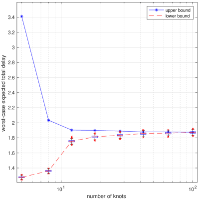
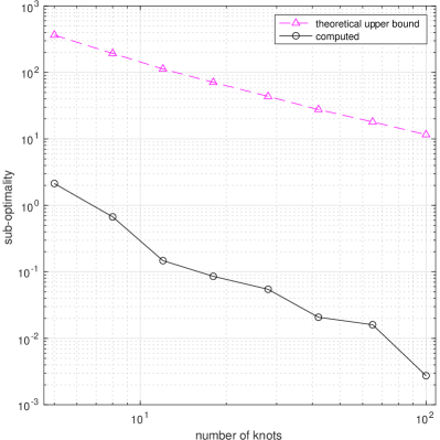
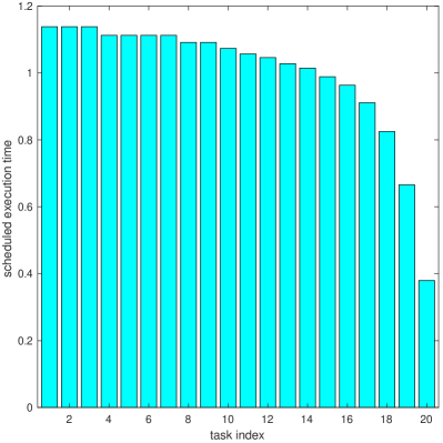
Figure 1: Results in the task scheduling example. Top-left: $\phi_{{\mathrm{D}\mathrm{R}\mathrm{O}}}^{\mathsf{U}\mathsf{B}}$ and $\phi_{{\mathrm{D}\mathrm{R}\mathrm{O}}}^{\mathsf{L}\mathsf{B}}$ versus the number of knots in each dimension (i.e., $m_{i,1}$). Top-right: $\hat{\epsilon}$ and a theoretical upper bound verses the number of knots in each dimension. Bottom: the approximately optimal scheduled execution time of the tasks.

Figure 1 shows the results of this numerical experiment. The top-left panel shows the values of $\phi_{{\mathrm{D}\mathrm{R}\mathrm{O}}}^{\mathsf{U}\mathsf{B}}$ and $\phi_{{\mathrm{D}\mathrm{R}\mathrm{O}}}^{\mathsf{L}\mathsf{B}}$ computed by Algorithm 3 as the number of knots increases from 5 to 100. By Theorem 4.8, $\phi_{{\mathrm{D}\mathrm{R}\mathrm{O}}}^{\mathsf{U}\mathsf{B}}$ and $\phi_{{\mathrm{D}\mathrm{R}\mathrm{O}}}^{\mathsf{L}\mathsf{B}}$ are upper and lower bounds for the optimal value $\phi_{{\mathrm{D}\mathrm{R}\mathrm{O}}}$ of ($\mathsf{DRO}$), where $\phi_{{\mathrm{D}\mathrm{R}\mathrm{O}}}$ corresponds to the optimized worst-case expected total delay of the tasks in this example. Since the lower bound $\phi_{{\mathrm{D}\mathrm{R}\mathrm{O}}}^{\mathsf{L}\mathsf{B}}$ was approximated by Monte Carlo integration, we show box plots of the 1000 approximate values from independent repetitions to visualize the Monte Carlo error. The result shows that, when the number of knots increased, both $\phi_{{\mathrm{D}\mathrm{R}\mathrm{O}}}^{\mathsf{U}\mathsf{B}}$ and $\phi_{{\mathrm{D}\mathrm{R}\mathrm{O}}}^{\mathsf{L}\mathsf{B}}$ improved drastically at first, and then gradually improved until they become very close. In fact, when at least 42 knots were used for each dimension, $\phi_{{\mathrm{D}\mathrm{R}\mathrm{O}}}^{\mathsf{U}\mathsf{B}}$ fell within the 95% Monte Carlo error bounds of $\phi_{{\mathrm{D}\mathrm{R}\mathrm{O}}}^{\mathsf{L}\mathsf{B}}$. When 100 knots were used for each dimension, the difference between $\phi_{{\mathrm{D}\mathrm{R}\mathrm{O}}}^{\mathsf{U}\mathsf{B}}$ and the mean of the approximate values of $\phi_{{\mathrm{D}\mathrm{R}\mathrm{O}}}^{\mathsf{L}\mathsf{B}}$ from the 1000 independent repetitions was around $2.7\times 10^{-3}$, which indicates that the approximately optimal solution $\hat{{\boldsymbol{a}}}$ computed by Algorithm 3 was very close to being optimal for this problem.

Next, to compare the sub-optimality estimate $\hat{\epsilon}$ computed from Algorithm 3 and its theoretical upper bound $\tilde{\epsilon}$ in Corollary 4.10, we plot the computed value of $\hat{\epsilon}$ and the value of a theoretical upper bound for $\hat{\epsilon}$ against the number of knots in the top-right panel of Figure 1. Specifically, this theoretical upper bound is computed as follows. For $i=1,\ldots,N$, we bound $\overline{W}_{1,\mu_{i}}\big{(}[\mu_{i}]_{\mathcal{G}_{i}}\big{)}$ from above by $\sum_{j=1}^{m_{i,1}}(\kappa_{i,1,(j+1)\wedge m_{i,1}}-\kappa_{i,1,(j-1)\vee 1})(\xi_{i,1,j}-\xi_{i,1,j-1})$ where $(\xi_{i,1,j})_{j=1:m_{i,1}}$ are defined as in (15); see also (7.21) in the proof of Proposition 3.14. Moreover, in this example, we have $\sup_{{\boldsymbol{\lambda}}\in S^{*}_{2}}\big{\{}\|\mathbf{W}^{\mathsf{T}}{\boldsymbol{\lambda}}\|_{\infty}\big{\}}=N$. Hence, the theoretical upper bound in the top-right panel of Figure 1 is given by $N\Big{(}\sum_{i=1}^{N}\sum_{j=1}^{m_{i,1}}(\kappa_{i,1,(j+1)\wedge m_{i,1}}-\kappa_{i,1,(j-1)\vee 1})(\xi_{i,1,j}-\xi_{i,1,j-1})\Big{)}$. It can be observed that the computed sub-optimality estimates are only around $0.02\%$ to $0.6\%$ of their respective theoretical upper bounds, which shows that the theoretical upper bounds are over-conservative. This confirms what we have discussed in Remark 4.12 and demonstrates the practicality of the iterative refinement strategy. This numerical example also showcases a valuable feature of the proposed method, as it produces computable upper and lower bounds for $\phi_{{\mathrm{D}\mathrm{R}\mathrm{O}}}$ as well as a practically reasonable estimate of the sub-optimality of the computed approximately optimal solution, without relying on over-conservative theoretical estimates.

Finally, the bottom panel of Figure 1 shows the approximately optimal solution $\hat{{\boldsymbol{a}}}$ of ($\mathsf{DRO}$) computed by Algorithm 3 when the number of knots is equal to 100 for each dimension. The approximately optimal solution corresponds to the scheduled duration of the 20 tasks. The result shows a decreasing pattern where earlier tasks are allocated more time compared to later tasks. This is due to the fact that the delay of an early task may lead to a chain reaction causing later tasks to be delayed.

5.2 Multi-product assembly (assemble-to-order system)

In this numerical example, we solve the distributionally robust multi-product assembly problem introduced in Example 2.5. We consider a manufacturer which produces 20 products that require 50 types of parts in total. The demand of each product is capped at 10 and is modeled by a random variable. As discussed in Example 2.5, we can formulate this problem into our two-stage DRO model in Assumption 2.1 with $K_{1}=50$, $K_{2}=70$, $N=20$, $\mathcal{X}_{1}=\mathcal{X}_{2}=\cdots=\mathcal{X}_{N}=[0,10]$, and $\mu_{1},\ldots,\mu_{N}\in\mathcal{P}([0,10])$. For $i=1,\ldots,N$, we let $\mu_{i}$ be a mixture of three equally weighted distributions, in which each mixture component is a truncated normal distribution with randomly generated parameters. Moreover, the per-unit prices and salvage values of the parts $c_{1}>s_{1}>0$, $\ldots$, $c_{50}>s_{50}>0$ and the per-unit returns from selling the products $q_{1}>0,\ldots,q_{20}>0$ are all randomly generated. The matrix $\mathbf{U}\in\mathbb{R}^{N\times K_{1}}$ that represents the type and amount of parts needed for producing each unit of product is a randomly generated sparse matrix with random entries.

Similar to Section 5.1, we adopt the iterative refinement strategy discussed in Remark 4.12 and vary $m_{i,1}$ from 5 to 100 for $i=1,\ldots,N$ (again, $k_{i}=1$ for $i=1,\ldots,N$ in this example). For each value of $m_{i,1}$, $\{\kappa_{i,1,1},\ldots,\kappa_{i,1,m_{i,1}}\}$ is again chosen by a greedy procedure. In Algorithm 3, we set $\epsilon=10^{-3}$ and approximate the expectation $\mathbb{E}\big{[}\langle\mathbf{W}\mkern 2.5mu\widetilde{\mkern-5.5mu{\boldsymbol{X}}\mkern-2.5mu}\mkern 2.5mu+{\boldsymbol{b}},{\boldsymbol{\lambda}}\rangle\big{]}$ in Line 3 via Monte Carlo integration where we generate $10^{7}$ independent samples using Algorithm 1. In addition, we independently repeat the Monte Carlo integration process 1000 times in order to quantify the Monte Carlo error.

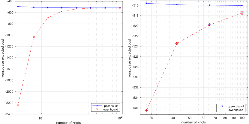
Figure 2: Results in the multi-product assembly example. Left: $\phi_{{\mathrm{D}\mathrm{R}\mathrm{O}}}^{\mathsf{U}\mathsf{B}}$ and $\phi_{{\mathrm{D}\mathrm{R}\mathrm{O}}}^{\mathsf{L}\mathsf{B}}$ versus the number of knots in each dimension (i.e., $m_{i,1}$). Right: magnification of the top-right part of the left panel.

The results of this numerical experiment are shown in Figure 2. The left panel shows the values of $\phi_{{\mathrm{D}\mathrm{R}\mathrm{O}}}^{\mathsf{U}\mathsf{B}}$ and $\phi_{{\mathrm{D}\mathrm{R}\mathrm{O}}}^{\mathsf{L}\mathsf{B}}$ computed by Algorithm 3 as the number of knots increases from 5 to 100, and the right panel shows a magnification of the top-right part of the left panel. Here, $\phi_{{\mathrm{D}\mathrm{R}\mathrm{O}}}^{\mathsf{U}\mathsf{B}}$ and $\phi_{{\mathrm{D}\mathrm{R}\mathrm{O}}}^{\mathsf{L}\mathsf{B}}$ are upper and lower bounds for $\phi_{{\mathrm{D}\mathrm{R}\mathrm{O}}}$, where $\phi_{{\mathrm{D}\mathrm{R}\mathrm{O}}}$ corresponds to the optimized worst-case expected value of the total cost of the parts minus the total return from selling the products and the unused parts. In the right panel of Figure 2, we show box plots of the 1000 independent Monte Carlo approximations of $\phi_{{\mathrm{D}\mathrm{R}\mathrm{O}}}^{\mathsf{L}\mathsf{B}}$ to visualize the Monte Carlo error. The result shows that, when the number of knots increased, both $\phi_{{\mathrm{D}\mathrm{R}\mathrm{O}}}^{\mathsf{U}\mathsf{B}}$ and $\phi_{{\mathrm{D}\mathrm{R}\mathrm{O}}}^{\mathsf{L}\mathsf{B}}$ improved drastically at first, and then gradually improved until they become very close. When 100 knots were used for each dimension, the difference between $\phi_{{\mathrm{D}\mathrm{R}\mathrm{O}}}^{\mathsf{U}\mathsf{B}}$ and the mean of the 1000 approximate values of $\phi_{{\mathrm{D}\mathrm{R}\mathrm{O}}}^{\mathsf{L}\mathsf{B}}$ from independent repetitions was around $1.45$, which is around $0.26\%$ of $|\phi_{{\mathrm{D}\mathrm{R}\mathrm{O}}}^{\mathsf{U}\mathsf{B}}|$. This indicates that the approximately optimal solution $\hat{{\boldsymbol{a}}}$ computed by Algorithm 3 was very close to being optimal for this problem. This observation is also in agreement with the results in the task scheduling example in Section 5.1.

5.3 Supply chain network design with uncertain demand and edge failure

In this numerical example, we solve the distributionally robust supply chain network design problem with uncertain demand and edge failure introduced in Example 2.6. We consider a supply chain network $(\mathtt{V},\mathtt{E})$ consisting of 15 suppliers, 20 processing facilities, and 10 customers, that is, $\mathtt{V}:=\mathtt{S}\cup\mathtt{P}\cup\mathtt{C}$ with $|\mathtt{S}|=15$, $|\mathtt{E}|=20$, $|\mathtt{C}|=10$. The edges $\mathtt{E}$ in the supply chain network are randomly generated. In total, there are 90 edges from the suppliers to the processing facilities and 60 edges from the processing facilities to the customers, that is, $\mathtt{E}:=\mathtt{E}_{\mathtt{S}\triangleright\mathtt{P}}\cup\mathtt{E}_{\mathtt{P}\triangleright\mathtt{C}}$ with $|\mathtt{E}_{\mathtt{S}\triangleright\mathtt{P}}|=90$, $|\mathtt{E}_{\mathtt{P}\triangleright\mathtt{C}}|=60$. For each customer $\mathtt{c}\in\mathtt{C}$, its demand $d_{\mathtt{c}}$ is modeled by a random variable with probability distribution $\mu_{\mathtt{c}}\in\mathcal{P}([0,2])$, which is a mixture of three equally weighted truncated normal distributions with randomly generated parameters. For each supplier $\mathtt{s}\in\mathtt{S}$, its supply $u_{\mathtt{s}}$ is randomly generated and then fixed. For each processing facility $\mathtt{p}\in\mathtt{P}$, its maximum processing capability $\overline{t}_{\mathtt{p}}$ is fixed at 2 and its investment cost $c^{(1)}_{\mathtt{p}}$ is randomly generated. Moreover, the transportation/processing costs of the edges, i.e., $\big{(}c^{(2)}_{\mathtt{s},\mathtt{p}}\big{)}_{(\mathtt{s},\mathtt{p})\in\mathtt{E}_{\mathtt{S}\triangleright\mathtt{P}}}$, $\big{(}c^{(2)}_{\mathtt{p},\mathtt{c}}\big{)}_{(\mathtt{p},\mathtt{c})\in\mathtt{E}_{\mathtt{P}\triangleright\mathtt{C}}}$, as well as their maximum transportation capacities, i.e., $(r_{\mathtt{s},\mathtt{p}})_{(\mathtt{s},\mathtt{p})\in\mathtt{E}_{\mathtt{S}\triangleright\mathtt{P}}}$, $(r_{\mathtt{p},\mathtt{c}})_{(\mathtt{p},\mathtt{c})\in\mathtt{E}_{\mathtt{P}\triangleright\mathtt{C}}}$, are randomly generated. Subsequently, we take the 15 edges from $\mathtt{E}_{\mathtt{S}\triangleright\mathtt{P}}$ with the least costs and the 10 edges from $\mathtt{E}_{\mathtt{P}\triangleright\mathtt{C}}$ with the least costs and set them to be susceptible to failure. Thus, we have $|\widetilde{\mathtt{E}}_{\mathtt{S}\triangleright\mathtt{P}}|=15$, $|\widetilde{\mathtt{E}}_{\mathtt{P}\triangleright\mathtt{C}}|=10$. The failure probabilities of these susceptible edges, i.e., $(\pi_{\mathtt{s},\mathtt{p}})_{(\mathtt{s},\mathtt{p})\in\widetilde{\mathtt{E}}_{\mathtt{S}\triangleright\mathtt{P}}}$, $(\pi_{\mathtt{p},\mathtt{c}})_{(\mathtt{p},\mathtt{c})\in\widetilde{\mathtt{E}}_{\mathtt{P}\triangleright\mathtt{C}}}$, are randomly generated. The configuration of this supply chain network is illustrated in the left panel of Figure 3, in which the suppliers are represented by magenta circles, the processing facilities are represented by blue circles, and the customers are represented by green circles. The sizes of the magenta circles represent the supplies $(u_{\mathtt{s}})_{\mathtt{s}\in\mathtt{S}}$, the sizes of the outer blue circles represent the maximum processing capabilities $(\overline{t}_{\mathtt{p}})_{\mathtt{p}\in\mathtt{P}}$, and the sizes of the green circles represent the mean values of the demands of the customers. In addition, the opacities of the outer blue circles represent the investment costs $\big{(}c^{(1)}_{\mathtt{p}}\big{)}_{\mathtt{p}\in\mathtt{P}}$ of the processing facilities, where an outer circle that is more opaque represents a higher investment cost. As for the edges, the widths represent their maximum transportation capacities $(r_{\mathtt{s},\mathtt{p}})_{(\mathtt{s},\mathtt{p})\in\mathtt{E}_{\mathtt{S}\triangleright\mathtt{P}}}$, $(r_{\mathtt{p},\mathtt{c}})_{(\mathtt{p},\mathtt{c})\in\mathtt{E}_{\mathtt{P}\triangleright\mathtt{C}}}$ and the opacities represent their costs $\big{(}c^{(2)}_{\mathtt{s},\mathtt{p}}\big{)}_{(\mathtt{s},\mathtt{p})\in\mathtt{E}_{\mathtt{S}\triangleright\mathtt{P}}}$, $\big{(}c^{(2)}_{\mathtt{p},\mathtt{c}}\big{)}_{(\mathtt{p},\mathtt{c})\in\mathtt{E}_{\mathtt{P}\triangleright\mathtt{C}}}$. The edges $\widetilde{\mathtt{E}}_{\mathtt{S}\triangleright\mathtt{P}}$, $\widetilde{\mathtt{E}}_{\mathtt{P}\triangleright\mathtt{C}}$ that are susceptible to failure are colored red, and their labels show their respective failure probabilities $(\pi_{\mathtt{s},\mathtt{p}})_{(\mathtt{s},\mathtt{p})\in\widetilde{\mathtt{E}}_{\mathtt{S}\triangleright\mathtt{P}}}$, $(\pi_{\mathtt{p},\mathtt{c}})_{(\mathtt{p},\mathtt{c})\in\widetilde{\mathtt{E}}_{\mathtt{P}\triangleright\mathtt{C}}}$ in percentage. As discussed in Example 2.6, we can formulate this problem into our two-stage DRO model in Assumption 2.1 with $K_{1}=170$, $K_{2}=150$, $N=35$, $\mathcal{X}_{1}=\mathcal{X}_{2}=\cdots=\mathcal{X}_{10}=[0,2]$, $\mu_{1},\ldots,\mu_{10}\in\mathcal{P}([0,2])$, $\mathcal{X}_{11}=\mathcal{X}_{12}=\cdots=\mathcal{X}_{35}=\{0,1\}$, and $\mu_{11},\ldots,\mu_{35}\in\mathcal{P}(\{0,1\})$.

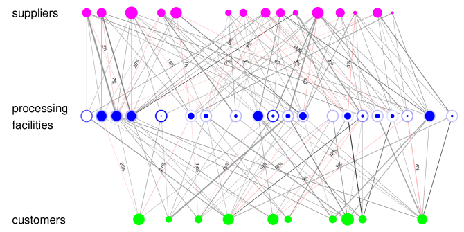
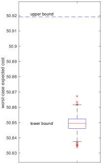
Figure 3: Results in the supply chain network design example. Left: the supply chain network configuration and the approximately optimal processing capabilities of the processing facilities. Right: $\phi_{{\mathrm{D}\mathrm{R}\mathrm{O}}}^{\mathsf{U}\mathsf{B}}$ and $\phi_{{\mathrm{D}\mathrm{R}\mathrm{O}}}^{\mathsf{L}\mathsf{B}}$.

Subsequently, we set $m_{i,1}=40$ for $i=1,\ldots,10$ (note that $k_{i}=1$ for $i=1,\ldots,10$ in this example). For $i=11,\ldots,35$, since $\mathcal{X}_{i}=\{0,1\}$, the conditions in (DRO1+) and (MS) require that $k_{i}=2$, $m_{i,1}=m_{i,2}=1$, and $\mathcal{G}_{i}=\mathcal{G}_{\mathrm{CPWA}}(0,1,\mathcal{X}_{i})$. In Algorithm 3, we set $\epsilon=10^{-2}$ and approximate the expectation $\mathbb{E}\big{[}\langle\mathbf{W}\mkern 2.5mu\widetilde{\mkern-5.5mu{\boldsymbol{X}}\mkern-2.5mu}\mkern 2.5mu+{\boldsymbol{b}},{\boldsymbol{\lambda}}\rangle\big{]}$ in Line 3 via Monte Carlo integration where we generate $10^{8}$ independent samples using Algorithm 1. In addition, we independently repeat the Monte Carlo integration process 1000 times in order to quantify the Monte Carlo error.

The values of $\phi_{{\mathrm{D}\mathrm{R}\mathrm{O}}}^{\mathsf{U}\mathsf{B}}$ and $\phi_{{\mathrm{D}\mathrm{R}\mathrm{O}}}^{\mathsf{L}\mathsf{B}}$ of this example computed by Algorithm 3 are shown in the right panel of Figure 3. They correspond to upper and lower bounds for $\phi_{{\mathrm{D}\mathrm{R}\mathrm{O}}}$, which is the optimized worst-case expected value of the total investment plus the total operational costs. Same as in Section 5.1 and Section 5.2, a box plot of the 1000 independent Monte Carlo approximations of $\phi_{{\mathrm{D}\mathrm{R}\mathrm{O}}}^{\mathsf{L}\mathsf{B}}$ is shown to visualize the Monte Carlo error. From the result, the difference between $\phi_{{\mathrm{D}\mathrm{R}\mathrm{O}}}^{\mathsf{U}\mathsf{B}}$ and the mean of the 1000 approximate values of $\phi_{{\mathrm{D}\mathrm{R}\mathrm{O}}}^{\mathsf{L}\mathsf{B}}$ from independent repetitions was around $0.07$, which is around $0.14\%$ of $\phi_{{\mathrm{D}\mathrm{R}\mathrm{O}}}^{\mathsf{U}\mathsf{B}}$. Hence, the approximately optimal solution $\hat{{\boldsymbol{a}}}$ computed by Algorithm 3 was very close to being optimal for this problem. This is again in agreement with the results in the examples in Section 5.1 and Section 5.2. Finally, the sizes of the inner blue circles in the left panel of Figure 3 represent the approximately optimal investments for the processing facilities, which is a sub-vector of $\hat{{\boldsymbol{a}}}$ computed by Algorithm 3.

AN gratefully acknowledges the financial support by his Nanyang Assistant Professorship Grant (NAP Grant) Machine Learning based Algorithms in Finance and Insurance.

Appendices

6 Proof of results in Section 2

Proof 6.1

Proof of Lemma 2.2 It follows from part (b) of the assumption (DRO3) that $Q({\boldsymbol{a}},{\boldsymbol{x}})$ corresponds to a feasible and bounded linear programming problem for all ${\boldsymbol{a}}\in S_{1}$ and all ${\boldsymbol{x}}\in{\boldsymbol{\mathcal{X}}}$. Statement (i) then follows from the strong duality of linear programming problems.

In the following, let

$$\begin{split}\mathbf{V}:=\left[\begin{tabular}[]{r}$\mathbf{V}_{\mathrm{i}\mathrm{n}}$\\ $\mathbf{V}_{\mathrm{e}\mathrm{q}}$\end{tabular}\right],\;\mathbf{W}:=\left[\begin{tabular}[]{r}$\mathbf{W}_{\mathrm{i}\mathrm{n}}$\\ $\mathbf{W}_{\mathrm{e}\mathrm{q}}$\end{tabular}\right],\;{\boldsymbol{b}}:=({\boldsymbol{b}}_{\mathrm{i}\mathrm{n}}^{\mathsf{T}},{\boldsymbol{b}}_{\mathrm{e}\mathrm{q}}^{\mathsf{T}})^{\mathsf{T}},\end{split}$$

for notational simplicity. It then follows from statement (i) that

$$Q({\boldsymbol{a}},{\boldsymbol{x}})=\sup_{{\boldsymbol{\lambda}}\in S_{2}^{*}}\big{\{}\langle\mathbf{V}{\boldsymbol{a}}+\mathbf{W}{\boldsymbol{x}}+{\boldsymbol{b}},{\boldsymbol{\lambda}}\rangle\big{\}}.$$ (6.1)

Subsequently, it follows from part (b) of the assumption (DRO3) that the linear maximization problem (6.1) is bounded above by some $\alpha\in\mathbb{R}$. Therefore, for every ${\boldsymbol{y}}\in\mathrm{r}\mathrm{e}\mathrm{c}(S^{*}_{2})$, every ${\boldsymbol{a}}\in S_{1}$, and every ${\boldsymbol{x}}\in{\boldsymbol{\mathcal{X}}}$, it holds that $\langle\mathbf{V}{\boldsymbol{a}}+\mathbf{W}{\boldsymbol{x}}+{\boldsymbol{b}},{\boldsymbol{y}}\rangle\leq 0$. By (Rockafellar 1970, p.170 & Theorem 19.1 & Theorem 19.5), the polyhedron $S^{*}_{2}$ can be expressed as $S^{*}_{2}=\mathrm{conv}\big{(}\{{\boldsymbol{\lambda}}_{1},\ldots,{\boldsymbol{\lambda}}_{k}\}\big{)}+\mathrm{r}\mathrm{e}\mathrm{c}(S^{*}_{2})$ for some $k\in\mathbb{N}$ and $\{{\boldsymbol{\lambda}}_{1},\ldots,{\boldsymbol{\lambda}}_{k}\}\subset S^{*}_{2}$. Consequently, one observes that $S^{*}_{2}$ in (6.1) can be replaced by $\overline{S}^{*}_{2}:=\mathrm{conv}\big{(}\{{\boldsymbol{\lambda}}_{1},\ldots,{\boldsymbol{\lambda}}_{k}\}\big{)}$ without changing the value of $Q({\boldsymbol{a}},{\boldsymbol{x}})$. Letting $B$ be any polytope that satisfies $B\supseteq\overline{S}^{*}_{2}$ completes the proof of statement (ii).

7 Proof of results in Section 3

7.1 Proof of results in Section 3.1

Proof 7.1

Proof of Lemma 3.1 Let us fix an arbitrary ${\boldsymbol{a}}\in S_{1}$. By the definition of $\phi(\cdot)$ in (2), we need to show that

$$\sup_{\mu\in\Gamma(\mu_{1},\ldots,\mu_{N})}\int_{{\boldsymbol{\mathcal{X}}}}Q({\boldsymbol{a}},{\boldsymbol{x}})\,{\mu}\!\left({\mathrm{d}{\boldsymbol{x}}}\right)\!=\sup_{\mu_{{\mathrm{a}\mathrm{u}\mathrm{g}}}\in\Gamma_{{\mathrm{a}\mathrm{u}\mathrm{g}}}(\mu_{1},\ldots,\mu_{N})}\int_{{\boldsymbol{\mathcal{X}}}\times S^{*}_{2}}Q_{{\mathrm{a}\mathrm{u}\mathrm{g}}}({\boldsymbol{a}},{\boldsymbol{x}},{\boldsymbol{\lambda}})\,{\mu_{{\mathrm{a}\mathrm{u}\mathrm{g}}}}\!\left({\mathrm{d}{\boldsymbol{x}},\mathrm{d}{\boldsymbol{\lambda}}}\right)\!.$$ (7.1)

Since the function ${\boldsymbol{\mathcal{X}}}\times S^{*}_{2}\ni({\boldsymbol{x}},{\boldsymbol{\lambda}})\mapsto Q_{{\mathrm{a}\mathrm{u}\mathrm{g}}}({\boldsymbol{a}},{\boldsymbol{x}},{\boldsymbol{\lambda}})\in\mathbb{R}$ is continuous and $S^{*}_{2}$ is compact, it follows from (Bertsekas and Shreve 1978, Proposition 7.33) that there exists a Borel measurable function ${\boldsymbol{\lambda}}^{\star}:{\boldsymbol{\mathcal{X}}}\to S^{*}_{2}$ such that

$$Q_{{\mathrm{a}\mathrm{u}\mathrm{g}}}({\boldsymbol{a}},{\boldsymbol{x}},{\boldsymbol{\lambda}}^{\star}({\boldsymbol{x}}))=\sup_{{\boldsymbol{\lambda}}\in S^{*}_{2}}\big{\{}Q_{{\mathrm{a}\mathrm{u}\mathrm{g}}}({\boldsymbol{a}},{\boldsymbol{x}},{\boldsymbol{\lambda}})\big{\}}=Q({\boldsymbol{a}},{\boldsymbol{x}})\qquad\forall{\boldsymbol{x}}\in{\boldsymbol{\mathcal{X}}}.$$ (7.2)

Now, let $\mu^{\star}\in\Gamma(\mu_{1},\ldots,\mu_{N})$ be an optimizer of the left-hand side of (7.1), which exists due to the boundedness and the continuity of the function ${\boldsymbol{\mathcal{X}}}\ni{\boldsymbol{x}}\mapsto Q({\boldsymbol{a}},{\boldsymbol{x}})\in\mathbb{R}$ as well as a multi-marginal extension of (Villani 2009, Theorem 4.1). Let $\mu^{\star}_{{\mathrm{a}\mathrm{u}\mathrm{g}}}\in\mathcal{P}({\boldsymbol{\mathcal{X}}}\times S^{*}_{2})$ be the push-forward of $\mu^{\star}$ under the mapping ${\boldsymbol{\mathcal{X}}}\ni{\boldsymbol{x}}\mapsto({\boldsymbol{x}},{\boldsymbol{\lambda}}^{\star}({\boldsymbol{x}}))\in{\boldsymbol{\mathcal{X}}}\times S^{*}_{2}$, i.e., $\mu^{\star}_{{\mathrm{a}\mathrm{u}\mathrm{g}}}:=\mu^{\star}\circ(\mathrm{i}\mathrm{d},{\boldsymbol{\lambda}}^{\star})^{-1}$ where $\mathrm{i}\mathrm{d}:{\boldsymbol{\mathcal{X}}}\to{\boldsymbol{\mathcal{X}}}$ denotes the identity mapping on ${\boldsymbol{\mathcal{X}}}$. It holds that $\mu^{\star}_{{\mathrm{a}\mathrm{u}\mathrm{g}}}\in\Gamma_{{\mathrm{a}\mathrm{u}\mathrm{g}}}(\mu_{1},\ldots,\mu_{N})$. Subsequently, it follows from (7.2) that

$$\int_{{\boldsymbol{\mathcal{X}}}\times S^{*}_{2}}Q_{{\mathrm{a}\mathrm{u}\mathrm{g}}}({\boldsymbol{a}},{\boldsymbol{x}},{\boldsymbol{\lambda}})\,{\mu^{\star}_{{\mathrm{a}\mathrm{u}\mathrm{g}}}}\!\left({\mathrm{d}{\boldsymbol{x}},\mathrm{d}{\boldsymbol{\lambda}}}\right)\!=\int_{{\boldsymbol{\mathcal{X}}}}Q_{{\mathrm{a}\mathrm{u}\mathrm{g}}}({\boldsymbol{a}},{\boldsymbol{x}},{\boldsymbol{\lambda}}^{\star}({\boldsymbol{x}}))\,{\mu^{\star}}\!\left({\mathrm{d}{\boldsymbol{x}}}\right)\!=\int_{{\boldsymbol{\mathcal{X}}}}Q({\boldsymbol{a}},{\boldsymbol{x}})\,{\mu^{\star}}\!\left({\mathrm{d}{\boldsymbol{x}}}\right)\!,$$

and thus the left-hand side of (7.1) is less than or equal to the right-hand side of (7.1). To prove the reverse inequality, let $\hat{\mu}_{{\mathrm{a}\mathrm{u}\mathrm{g}}}\in\Gamma_{{\mathrm{a}\mathrm{u}\mathrm{g}}}(\mu_{1},\ldots,\mu_{N})$ be arbitrary and let $\hat{\mu}$ be the marginal of $\hat{\mu}_{{\mathrm{a}\mathrm{u}\mathrm{g}}}$ on ${\boldsymbol{\mathcal{X}}}$. It thus holds that $\hat{\mu}\in\Gamma(\mu_{1},\ldots,\mu_{N})$. Moreover, since $Q_{{\mathrm{a}\mathrm{u}\mathrm{g}}}({\boldsymbol{a}},{\boldsymbol{x}},{\boldsymbol{\lambda}})\leq Q({\boldsymbol{a}},{\boldsymbol{x}})$ for all ${\boldsymbol{x}}\in{\boldsymbol{\mathcal{X}}}$ and all ${\boldsymbol{\lambda}}\in S^{*}_{2}$, it holds that

$$\int_{{\boldsymbol{\mathcal{X}}}\times S^{*}_{2}}Q_{{\mathrm{a}\mathrm{u}\mathrm{g}}}({\boldsymbol{a}},{\boldsymbol{x}},{\boldsymbol{\lambda}})\,{\hat{\mu}_{{\mathrm{a}\mathrm{u}\mathrm{g}}}}\!\left({\mathrm{d}{\boldsymbol{x}},\mathrm{d}{\boldsymbol{\lambda}}}\right)\!\leq\int_{{\boldsymbol{\mathcal{X}}}\times S^{*}_{2}}Q({\boldsymbol{a}},{\boldsymbol{x}})\,{\hat{\mu}_{{\mathrm{a}\mathrm{u}\mathrm{g}}}}\!\left({\mathrm{d}{\boldsymbol{x}},\mathrm{d}{\boldsymbol{\lambda}}}\right)\!=\int_{{\boldsymbol{\mathcal{X}}}}Q({\boldsymbol{a}},{\boldsymbol{x}})\,{\hat{\mu}}\!\left({\mathrm{d}{\boldsymbol{x}}}\right)\!.$$

This shows that the right-hand side of (7.1) is less than or equal to the left-hand side of (7.1). Finally, (8) follows from (7) and ($\mathsf{DRO}$). The proof is now complete.

Proof 7.2

Proof of Lemma 3.5 This result follows from the gluing lemma (see, e.g., (Villani 2009, Lemma 7.6)) and an inductive argument similar to the proof of (Neufeld and Xiang 2022, Lemma 2.2.3).

Proof 7.3

Proof of Theorem 3.7 This proof is adapted from the proof of (Neufeld and Xiang 2022, Theorem 2.2.8). To prove statement (i), let us fix an arbitrary $\hat{\mu}_{{\mathrm{a}\mathrm{u}\mathrm{g}}}\in\Gamma_{{\mathrm{a}\mathrm{u}\mathrm{g}}}([\mu_{1}]_{\mathcal{G}_{1}},\ldots,[\mu_{N}]_{\mathcal{G}_{N}})$. For $i=1,\ldots,N$, let $\hat{\mu}_{i}$ denote the marginal of $\hat{\mu}_{{\mathrm{a}\mathrm{u}\mathrm{g}}}$ on $\mathcal{X}_{i}$ and let $\bar{\mathcal{X}}_{i}:=\mathcal{X}_{i}$. We have by (11) and (6) that $\hat{\mu}_{i}\in[\mu_{i}]_{\mathcal{G}_{i}}$. By the assumption that $\tilde{\mu}_{{\mathrm{a}\mathrm{u}\mathrm{g}}}\in R_{\mathrm{part}}(\hat{\mu}_{{\mathrm{a}\mathrm{u}\mathrm{g}}};\mu_{1},\ldots,\mu_{N})$ and Definition 3.4, there exists a probability measure $\gamma\in\mathcal{P}({\mathcal{X}_{1}\times\cdots\times\mathcal{X}_{N}}\times{\bar{\mathcal{X}}_{1}\times\cdots\times\bar{\mathcal{X}}_{N}}\times S^{*}_{2})$, such that the marginal of $\gamma$ on $\mathcal{X}_{1}\times\cdots\times\mathcal{X}_{N}\times S^{*}_{2}$ is $\hat{\mu}_{{\mathrm{a}\mathrm{u}\mathrm{g}}}$, the marginal $\gamma_{i}\in\Gamma(\hat{\mu}_{i},\mu_{i})$ of $\gamma$ on $\mathcal{X}_{i}\times\bar{\mathcal{X}}_{i}$ satisfies $\int_{\mathcal{X}_{i}\times\bar{\mathcal{X}}_{i}}{|x-\bar{x}|}\,{\gamma_{i}}\!\left({\mathrm{d}x,\mathrm{d}\bar{x}}\right)\!=W_{1}(\hat{\mu}_{i},\mu_{i})$ for $i=1,\ldots,N$, and the marginal of $\gamma$ on $\bar{\mathcal{X}}_{1}\times\cdots\times\bar{\mathcal{X}}_{N}\times S^{*}_{2}$ is $\tilde{\mu}_{{\mathrm{a}\mathrm{u}\mathrm{g}}}$. Let $\mkern 6.5mu\overline{\mkern-5.5mu{\boldsymbol{\mathcal{X}}}\mkern-2.5mu}\mkern 2.5mu:=\bar{\mathcal{X}}_{1}\times\cdots\times\bar{\mathcal{X}}_{N}$. We have

$$\begin{split}&\phantom{=}\;\int_{{\boldsymbol{\mathcal{X}}}\times S^{*}_{2}}\langle\mathbf{W}{\boldsymbol{x}}+{\boldsymbol{b}},{\boldsymbol{\lambda}}\rangle\,{\hat{\mu}_{{\mathrm{a}\mathrm{u}\mathrm{g}}}}\!\left({\mathrm{d}{\boldsymbol{x}},\mathrm{d}{\boldsymbol{\lambda}}}\right)\!-\int_{{\boldsymbol{\mathcal{X}}}\times S^{*}_{2}}\langle\mathbf{W}{\boldsymbol{x}}+{\boldsymbol{b}},{\boldsymbol{\lambda}}\rangle\,{\tilde{\mu}_{{\mathrm{a}\mathrm{u}\mathrm{g}}}}\!\left({\mathrm{d}{\boldsymbol{x}},\mathrm{d}{\boldsymbol{\lambda}}}\right)\!\\ &=\int_{{\boldsymbol{\mathcal{X}}}\times\mkern 6.5mu\overline{\mkern-5.5mu{\boldsymbol{\mathcal{X}}}\mkern-2.5mu}\mkern 2.5mu\times S^{*}_{2}}\langle\mathbf{W}{\boldsymbol{x}}+{\boldsymbol{b}},{\boldsymbol{\lambda}}\rangle-\langle\mathbf{W}\bar{{\boldsymbol{x}}}+{\boldsymbol{b}},{\boldsymbol{\lambda}}\rangle\,{\gamma}\!\left({\mathrm{d}{\boldsymbol{x}},\mathrm{d}\bar{{\boldsymbol{x}}},\mathrm{d}{\boldsymbol{\lambda}}}\right)\!\\ &=\int_{{\boldsymbol{\mathcal{X}}}\times\mkern 6.5mu\overline{\mkern-5.5mu{\boldsymbol{\mathcal{X}}}\mkern-2.5mu}\mkern 2.5mu\times S^{*}_{2}}\langle\mathbf{W}^{\mathsf{T}}{\boldsymbol{\lambda}},{\boldsymbol{x}}-\bar{{\boldsymbol{x}}}\rangle\,{\gamma}\!\left({\mathrm{d}{\boldsymbol{x}},\mathrm{d}\bar{{\boldsymbol{x}}},\mathrm{d}{\boldsymbol{\lambda}}}\right)\!\\ &\leq\sup_{{\boldsymbol{\lambda}}\in S^{*}_{2}}\big{\{}\|\mathbf{W}^{\mathsf{T}}{\boldsymbol{\lambda}}\|_{\infty}\big{\}}\int_{{\boldsymbol{\mathcal{X}}}\times\mkern 6.5mu\overline{\mkern-5.5mu{\boldsymbol{\mathcal{X}}}\mkern-2.5mu}\mkern 2.5mu\times S^{*}_{2}}\|{\boldsymbol{x}}-\bar{{\boldsymbol{x}}}\|_{1}\,{\gamma}\!\left({\mathrm{d}{\boldsymbol{x}},\mathrm{d}\bar{{\boldsymbol{x}}},\mathrm{d}{\boldsymbol{\lambda}}^{\prime}}\right)\!\\ &=\sup_{{\boldsymbol{\lambda}}\in S^{*}_{2}}\big{\{}\|\mathbf{W}^{\mathsf{T}}{\boldsymbol{\lambda}}\|_{\infty}\big{\}}\left(\sum_{i=1}^{N}\int_{\mathcal{X}_{i}\times\bar{\mathcal{X}}_{i}}|x_{i}-\bar{x}_{i}|\,{\gamma_{i}}\!\left({\mathrm{d}x_{i},\mathrm{d}\bar{x}_{i}}\right)\!\right)\\ &=\sup_{{\boldsymbol{\lambda}}\in S^{*}_{2}}\big{\{}\|\mathbf{W}^{\mathsf{T}}{\boldsymbol{\lambda}}\|_{\infty}\big{\}}\left(\sum_{i=1}^{N}W_{1}(\hat{\mu}_{i},\mu_{i})\right)\\ &\leq\sup_{{\boldsymbol{\lambda}}\in S^{*}_{2}}\big{\{}\|\mathbf{W}^{\mathsf{T}}{\boldsymbol{\lambda}}\|_{\infty}\big{\}}\left(\sum_{i=1}^{N}\overline{W}_{1,\mu_{i}}([\mu_{i}]_{\mathcal{G}_{i}})\right)\\ &=\bar{\epsilon}.\end{split}$$ (7.3)

This proves statement (i).

To prove statement (ii), let us fix an arbitrary ${\boldsymbol{a}}\in S_{1}$. Since $\Gamma_{{\mathrm{a}\mathrm{u}\mathrm{g}}}(\mu_{1},\ldots,\mu_{N})\subset\Gamma_{{\mathrm{a}\mathrm{u}\mathrm{g}}}([\mu_{1}]_{\mathcal{G}_{1}},\ldots,[\mu_{N}]_{\mathcal{G}_{N}})$, we have

$$\begin{split}\sup_{\mu_{{\mathrm{a}\mathrm{u}\mathrm{g}}}\in\Gamma_{{\mathrm{a}\mathrm{u}\mathrm{g}}}([\mu_{1}]_{\mathcal{G}_{1}},\ldots,[\mu_{N}]_{\mathcal{G}_{N}})}&\bigg{\{}\int_{{\boldsymbol{\mathcal{X}}}\times S^{*}_{2}}Q_{{\mathrm{a}\mathrm{u}\mathrm{g}}}({\boldsymbol{a}},{\boldsymbol{x}},{\boldsymbol{\lambda}})\,{\mu_{{\mathrm{a}\mathrm{u}\mathrm{g}}}}\!\left({\mathrm{d}{\boldsymbol{x}},\mathrm{d}{\boldsymbol{\lambda}}}\right)\!\bigg{\}}\\ &\geq\sup_{\mu_{{\mathrm{a}\mathrm{u}\mathrm{g}}}\in\Gamma_{{\mathrm{a}\mathrm{u}\mathrm{g}}}(\mu_{1},\ldots,\mu_{N})}\bigg{\{}\int_{{\boldsymbol{\mathcal{X}}}\times S^{*}_{2}}Q_{{\mathrm{a}\mathrm{u}\mathrm{g}}}({\boldsymbol{a}},{\boldsymbol{x}},{\boldsymbol{\lambda}})\,{\mu_{{\mathrm{a}\mathrm{u}\mathrm{g}}}}\!\left({\mathrm{d}{\boldsymbol{x}},\mathrm{d}{\boldsymbol{\lambda}}}\right)\!\bigg{\}}.\end{split}$$ (7.4)

Statement (ii) then follows by combining (5), (7.3), (14), and (7.4).

Next, let us prove statement (iii). Let us fix an arbitrary ${\boldsymbol{a}}\in S_{1}$ as well as an arbitrary $\hat{\mu}_{{\mathrm{a}\mathrm{u}\mathrm{g}}}\in\Gamma_{{\mathrm{a}\mathrm{u}\mathrm{g}}}([\mu_{1}]_{\mathcal{G}_{1}},\ldots,[\mu_{N}]_{\mathcal{G}_{N}})$, and let $\tilde{\mu}_{{\mathrm{a}\mathrm{u}\mathrm{g}}}\in R_{\mathrm{part}}(\hat{\mu}_{{\mathrm{a}\mathrm{u}\mathrm{g}}};\mu_{1},\ldots,\mu_{N})$. Since $\tilde{\mu}_{{\mathrm{a}\mathrm{u}\mathrm{g}}}\in\Gamma_{{\mathrm{a}\mathrm{u}\mathrm{g}}}(\mu_{1},\ldots,\mu_{N})$, it follows from (5) and statement (i) that

$$\begin{split}&\phantom{=}\;\int_{{\boldsymbol{\mathcal{X}}}\times S^{*}_{2}}Q_{{\mathrm{a}\mathrm{u}\mathrm{g}}}({\boldsymbol{a}},{\boldsymbol{x}},{\boldsymbol{\lambda}})\,{\hat{\mu}_{{\mathrm{a}\mathrm{u}\mathrm{g}}}}\!\left({\mathrm{d}{\boldsymbol{x}},\mathrm{d}{\boldsymbol{\lambda}}}\right)\!-\bar{\epsilon}\\ &\leq\int_{{\boldsymbol{\mathcal{X}}}\times S^{*}_{2}}Q_{{\mathrm{a}\mathrm{u}\mathrm{g}}}({\boldsymbol{a}},{\boldsymbol{x}},{\boldsymbol{\lambda}})\,{\tilde{\mu}_{{\mathrm{a}\mathrm{u}\mathrm{g}}}}\!\left({\mathrm{d}{\boldsymbol{x}},\mathrm{d}{\boldsymbol{\lambda}}}\right)\!\\ &\leq\sup_{\mu_{{\mathrm{a}\mathrm{u}\mathrm{g}}}\in\Gamma_{{\mathrm{a}\mathrm{u}\mathrm{g}}}(\mu_{1},\ldots,\mu_{N})}\bigg{\{}\int_{{\boldsymbol{\mathcal{X}}}\times S^{*}_{2}}Q_{{\mathrm{a}\mathrm{u}\mathrm{g}}}({\boldsymbol{a}},{\boldsymbol{x}},{\boldsymbol{\lambda}})\,{\mu_{{\mathrm{a}\mathrm{u}\mathrm{g}}}}\!\left({\mathrm{d}{\boldsymbol{x}},\mathrm{d}{\boldsymbol{\lambda}}}\right)\!\bigg{\}}.\end{split}$$ (7.5)

Taking supremum over $\hat{\mu}_{{\mathrm{a}\mathrm{u}\mathrm{g}}}\in\Gamma_{{\mathrm{a}\mathrm{u}\mathrm{g}}}([\mu_{1}]_{\mathcal{G}_{1}},\ldots,[\mu_{N}]_{\mathcal{G}_{N}})$ and then adding $\langle{\boldsymbol{c}}_{1},{\boldsymbol{a}}\rangle$ to the two sides of (7.5) yields $\phi_{{\mathrm{s}\mathrm{u}\mathrm{r}}}({\boldsymbol{a}})-\bar{\epsilon}\leq\phi({\boldsymbol{a}})$. The other inequality $\phi({\boldsymbol{a}})\leq\phi_{{\mathrm{s}\mathrm{u}\mathrm{r}}}({\boldsymbol{a}})$ follows from (7.4).

Finally, statement (iv) follows from statement (iii) by taking infimum over ${\boldsymbol{a}}\in S_{1}$. The proof is now complete.

7.2 Proof of results in Section 3.2

Before proving Proposition 3.9, let us first prove the following lemma. This lemma will also be used later in the proof of Proposition 3.11 as well as the proof of Proposition 3.14.

Lemma 7.4 (Characterization of an optimal coupling in one dimension)

Let $\mathcal{X}\subset\mathbb{R}$ be compact, let $\mu\in\mathcal{P}(\mathcal{X})$, and let $F_{\mu}:\overline{\mathbb{R}}\to[0,1]$ be defined as

$$F_{\mu}(z):=\mu\big{(}\mathcal{X}\cap(-\infty,x]\big{)}\qquad\forall x\in\overline{\mathbb{R}}.$$

Moreover, let $F^{-1}_{\mu}:[0,1]\to\mathcal{X}$ be defined as

$$F^{-1}_{\mu}(t):=\inf\big{\{}x\in\mathcal{X}:F_{\mu}(x)\geq t\big{\}}\qquad\forall t\in[0,1].$$

Then, the following statements hold.

1. $F^{-1}_{\mu}(t)=\inf\big{\{}z\in\mathbb{R}:F_{\mu}(z)\geq t\big{\}}$ for all $t\in(0,1]$.

2. If $(\Omega,\mathcal{F},\mathbb{P})$ is a probability space, $U:\Omega\to[0,1]$ is a random variable with the uniform distribution, and $X:\Omega\to\mathcal{X}$ is a random variable defined as $X:=F^{-1}_{\mu}(U)$, then $\mathbbm{1}_{\{X\leq x\}}=\mathbbm{1}_{\{U\leq F_{\mu}(x)\}}$ $\mathbb{P}$–a.s. for all $x\in\overline{\mathbb{R}}$ and the law of $X$ is $\mu$.

Let $\nu\in\mathcal{P}(\mathcal{X})$ and let $F_{\nu}(\cdot)$, $F^{-1}_{\nu}(\cdot)$ be defined as $F_{\mu}(\cdot)$, $F^{-1}_{\mu}(\cdot)$ but with respect to $\nu$. Then, the following statements hold.

1. $W_{1}(\mu,\nu)=\int_{[0,1]}|F^{-1}_{\mu}(t)-F^{-1}_{\nu}(t)|\,\mathrm{d}{t}$.

2. If $(\Omega,\mathcal{F},\mathbb{P})$ is a probability space, $U:\Omega\to[0,1]$ is a random variable with the uniform distribution, $X:\Omega\to\mathcal{X}$ is a random variable defined as $X:=F^{-1}_{\mu}(U)$, $Y:\Omega\to\mathcal{X}$ is a random variable defined as $Y:=F^{-1}_{\nu}(U)$, and $\gamma\in\mathcal{P}(\mathcal{X}\times\mathcal{X})$ is the law of the random vector $(X,Y)^{\mathsf{T}}$, then $\gamma\in\Gamma(\mu,\nu)$ and $W_{1}(\mu,\nu)=\int_{\mathcal{X}\times\mathcal{X}}|x-y|\,{\gamma}\!\left({\mathrm{d}x,\mathrm{d}y}\right)\!$.

Proof 7.5

Proof of Lemma 7.4 Let us define $\widetilde{F}^{-1}_{\mu}(t):=\inf\big{\{}z\in\mathbb{R}:F_{\mu}(z)\geq t\big{\}}$ for $t\in[0,1]$. Since $\mathcal{X}$ is bounded, it holds that $\widetilde{F}^{-1}_{\mu}(t)\in\mathbb{R}$ for all $t\in(0,1]$. It follows from the definitions that $\widetilde{F}^{-1}_{\mu}(t)\leq F^{-1}_{\mu}(t)$ for all $t\in(0,1]$. Suppose, for the sake of contradiction, that there exists $\hat{t}\in(0,1]$ such that $F^{-1}_{\mu}(\hat{t})>\widetilde{F}^{-1}_{\mu}(\hat{t})=:\hat{y}\in\mathbb{R}$. Then, it follows from the monotonicity and the right continuity of the function $F_{\mu}(\cdot)$ that $F_{\mu}(z)\geq\hat{t}$ for all $z\geq\hat{y}$. Since $\hat{y}<F^{-1}_{\mu}(\hat{t})$, this implies that $\hat{y}\notin\mathcal{X}$. Subsequently, it follows from the closedness of $\mathcal{X}$ that there exists $\epsilon>0$ such that $(\hat{y}-\epsilon,\hat{y}]\subset\mathbb{R}\setminus\mathcal{X}$, and thus $\hat{t}\leq F_{\mu}(\hat{y})=\mu\big{(}\mathcal{X}\cap(-\infty,\hat{y}]\big{)}=\mu\big{(}\mathcal{X}\cap(-\infty,\hat{y}-\epsilon]\big{)}+\mu\big{(}\mathcal{X}\cap(\hat{y}-\epsilon,\hat{y}]\big{)}=\mu\big{(}\mathcal{X}\cap(-\infty,\hat{y}-\epsilon]\big{)}=F_{\mu}(\hat{y}-\epsilon)$. This contradicts the assumption that $\hat{y}=\widetilde{F}^{-1}_{\mu}(\hat{t})=\inf\big{\{}z\in\mathbb{R}:F_{\mu}(z)\geq\hat{t}\big{\}}$. The proof of statement (i) is complete.

To prove statement (ii), let us define $\widetilde{X}:\Omega\to\overline{\mathbb{R}}$ by $\widetilde{X}:=\widetilde{F}^{-1}_{\mu}(U)$. We have for all $x\in\overline{\mathbb{R}}$ that

$$\widetilde{X}=\widetilde{F}^{-1}_{\mu}(U)\leq x \quad\Rightarrow\quad U\leq F_{\mu}(\widetilde{F}^{-1}_{\mu}(U))\leq F_{\mu}(x),$$

$$U\leq F_{\mu}(x) \quad\Rightarrow\quad\widetilde{X}=\widetilde{F}^{-1}_{\mu}(U)\leq\widetilde{F}^{-1}_{\mu}(F_{\mu}(x))\leq x,$$

where we have used the non-decreasing property of $F_{\mu}$, $\widetilde{F}^{-1}_{\mu}$, and the two inequalities: $U\leq F_{\mu}(\widetilde{F}^{-1}_{\mu}(U))$, $\widetilde{F}^{-1}_{\mu}(F_{\mu}(x))\leq x$, which are consequences of statements (vi) and (v) in (McNeil et al. 2005, Proposition A.3). Hence, we have for all $x\in\overline{\mathbb{R}}$ that $\mathbbm{1}_{\{\widetilde{X}\leq x\}}(\omega)=\mathbbm{1}_{\{U\leq F_{\mu}(x)\}}(\omega)$ for all $\omega\in\Omega$. Moreover, since $\widetilde{F}^{-1}_{\mu}(0)=-\infty$ and $F^{-1}_{\mu}(0)=\min\{x:x\in\mathcal{X}\}>-\infty$, we have by statement (i) that ${\{\widetilde{X}\neq X\}}=\{U=0\}$. Since $U$ has the uniform distribution on $[0,1]$, $\mathbb{P}[U=0]=0$, and thus $\mathbbm{1}_{\{X\leq x\}}=\mathbbm{1}_{\{U\leq F_{\mu}(x)\}}$ $\mathbb{P}$–a.s. for all $x\in\overline{\mathbb{R}}$. This also implies that $\mathbb{P}[{X\leq x}]=\mathbb{P}[{U\leq F_{\mu}(x)}]=F_{\mu}(x)$ for all $x\in\overline{\mathbb{R}}$ and hence the law of $X$ is $\mu$. This completes the proof of statement (ii).

Next, let us prove statements (iii) and (iv). To that end, let us make the assumptions in statement (iv). It follows from statement (ii) that $\gamma\in\Gamma(\mu,\nu)$. Let $\gamma^{\dagger}\in\mathcal{P}(\mathbb{R}^{2})$ be defined by $\gamma^{\dagger}(E):=\gamma\big{(}(\mathcal{X}\times\mathcal{X})\cap E\big{)}$ for all $E\in\mathcal{B}(\mathbb{R}^{2})$. Similarly, let us define $\mu^{\dagger},\nu^{\dagger}\in\mathcal{P}(\mathbb{R})$ by $\mu^{\dagger}(E):=\mu(\mathcal{X}\cap E)$ and $\nu^{\dagger}(E):=\nu(\mathcal{X}\cap E)$ for all $E\in\mathcal{B}(\mathbb{R})$. Then, it holds that $\gamma^{\dagger}\in\Gamma(\mu^{\dagger},\nu^{\dagger})$. Moreover, let $\widetilde{F}^{-1}_{\nu}(t):=\inf\big{\{}z\in\mathbb{R}:F_{\nu}(z)\geq t\big{\}}$ for $t\in[0,1]$. Notice that $F_{\mu}(z)=\mu^{\dagger}\big{(}(-\infty,z]\big{)}$ and $F_{\nu}(z)=\nu^{\dagger}\big{(}(-\infty,z]\big{)}$ for all $z\in\overline{\mathbb{R}}$. We have

$$\begin{split}\int_{\mathbb{R}\times\mathbb{R}}|x-y|\,{\gamma^{\dagger}}\!\left({\mathrm{d}x,\mathrm{d}y}\right)\!&=\int_{\mathcal{X}\times\mathcal{X}}|x-y|\,{\gamma}\!\left({\mathrm{d}x,\mathrm{d}y}\right)\!\\ &=\mathbb{E}[|X-Y|]\\ &=\mathbb{E}\big{[}\big{|}F^{-1}_{\mu}(U)-F^{-1}_{\nu}(U)\big{|}\big{]}\\ &=\int_{[0,1]}\big{|}F^{-1}_{\mu}(t)-F^{-1}_{\nu}(t)\big{|}\,\mathrm{d}{t}\\ &=\int_{(0,1)}\big{|}F^{-1}_{\mu}(t)-F^{-1}_{\nu}(t)\big{|}\,\mathrm{d}{t}\\ &=\int_{(0,1)}\big{|}\widetilde{F}^{-1}_{\mu}(t)-\widetilde{F}^{-1}_{\nu}(t)\big{|}\,\mathrm{d}{t}\\ &\leq W_{1}(\mu^{\dagger},\nu^{\dagger}),\end{split}$$

where the last equality follows from statement (i) and the inequality follows from (Rachev and Rüschendorf 1998, Equation (3.1.6)). This shows that

$$\int_{\mathbb{R}\times\mathbb{R}}|x-y|\,{\gamma^{\dagger}}\!\left({\mathrm{d}x,\mathrm{d}y}\right)\! =\int_{\mathcal{X}\times\mathcal{X}}|x-y|\,{\gamma}\!\left({\mathrm{d}x,\mathrm{d}y}\right)\!=\int_{[0,1]}\big{|}F^{-1}_{\mu}(t)-F^{-1}_{\nu}(t)\big{|}\,\mathrm{d}{t}=W_{1}(\mu^{\dagger},\nu^{\dagger}).$$ (7.6)

Now, let $\eta\in\Gamma(\mu,\nu)$ be arbitrary and let $\eta^{\dagger}\in\mathcal{P}(\mathbb{R}^{2})$ be defined by $\eta^{\dagger}(E):=\eta\big{(}(\mathcal{X}\times\mathcal{X})\cap E\big{)}$ for all $E\in\mathcal{B}(\mathbb{R}^{2})$. Subsequently, since $\eta^{\dagger}\in\Gamma(\mu^{\dagger},\nu^{\dagger})$, we have by (7.6) that

$$\int_{\mathcal{X}\times\mathcal{X}}|x-y|\,{\eta}\!\left({\mathrm{d}x,\mathrm{d}y}\right)\! =\int_{\mathbb{R}\times\mathbb{R}}|x-y|\,{\eta^{\dagger}}\!\left({\mathrm{d}x,\mathrm{d}y}\right)\!$$

$$\geq W_{1}(\mu^{\dagger},\nu^{\dagger})$$

$$=\int_{[0,1]}\big{|}F^{-1}_{\mu}(t)-F^{-1}_{\nu}(t)\big{|}\,\mathrm{d}{t}$$

$$=\int_{\mathcal{X}\times\mathcal{X}}|x-y|\,{\gamma}\!\left({\mathrm{d}x,\mathrm{d}y}\right)\!,$$

which proves that $\int_{\mathcal{X}\times\mathcal{X}}|x-y|\,{\gamma}\!\left({\mathrm{d}x,\mathrm{d}y}\right)\!=\int_{[0,1]}|F^{-1}_{\mu}(t)-F^{-1}_{\nu}(t)|\,\mathrm{d}{t}=W_{1}(\mu,\nu)$. This proves statements (iii) and (iv). The proof is now complete.

Proof 7.6

Proof of Proposition 3.9 Statement (i) follows from Sklar’s theorem in the copula theory (see, e.g., McNeil et al. (2005, Theorem 5.3)). Let us prove statement (ii). For $j=1,\ldots,K^{*}_{2}$, let $\pi_{j}(S^{*}_{2})\subset\mathbb{R}$ denote the projection of $S^{*}_{2}$ onto the $j$-th coordinate, which is a compact interval since $S^{*}_{2}$ is a polytope. Subsequently, let $\hat{\mu}_{i}\in\mathcal{P}(\mathcal{X}_{i})$ denote the marginal of $\hat{\mu}_{{\mathrm{a}\mathrm{u}\mathrm{g}}}$ on $\mathcal{X}_{i}$ for $i=1,\ldots,N$, and let $\hat{\mu}_{N+j}\in\mathcal{P}(\pi_{j}(S^{*}_{2}))$ denote the marginal of $\hat{\mu}_{{\mathrm{a}\mathrm{u}\mathrm{g}}}$ on the $(N+j)$-th coordinate for $j=1,\ldots,K^{*}_{2}$. It thus holds for $i=1,\ldots,N$ and all $z\in\overline{\mathbb{R}}$ that $F_{\hat{\mu}_{i}}(z)=\hat{\mu}_{i}\big{(}\mathcal{X}_{i}\cap(-\infty,z]\big{)}$ and $F_{\mu_{i}}(z)=\mu_{i}\big{(}\mathcal{X}_{i}\cap(-\infty,z]\big{)}$. It also holds for $j=1,\ldots,K^{*}_{2}$ and all $z\in\overline{\mathbb{R}}$ that $F_{\hat{\mu}_{N+j}}(z)=\hat{\mu}_{N+j}\big{(}\pi_{j}(S^{*}_{2})\cap(-\infty,z]\big{)}$. Now, let $F^{-1}_{\hat{\mu}_{i}}(t):=\inf\big{\{}x\in\mathcal{X}_{i}:F_{\hat{\mu}_{i}}(x)\geq t\big{\}}$, $F^{-1}_{\mu_{i}}(t):=\inf\big{\{}x\in\mathcal{X}_{i}:F_{\mu_{i}}(x)\geq t\big{\}}$ for $t\in[0,1]$ and $i=1,\ldots,N$, and let $F^{-1}_{\hat{\mu}_{N+j}}(t):=\inf\big{\{}\lambda\in\pi_{j}(S^{*}_{2}):F_{\hat{\mu}_{N+j}}(\lambda)\geq t\big{\}}$ for $t\in[0,1]$ and $j=1,\ldots,K^{*}_{2}$. Moreover, let $(\Omega,\mathcal{F},\mathbb{P})$ be a probability space and let $(U_{1},\ldots,U_{N},V_{1},\ldots,V_{K^{*}_{2}})^{\mathsf{T}}:\Omega\to[0,1]^{N+K^{*}_{2}}$ be a random vector with distribution function $C$. Consequently, $U_{1},\ldots,U_{N},V_{1},\ldots,V_{K^{*}_{2}}$ are all uniform random variables on $[0,1]$. For $i=1,\ldots,N$, let $X_{i}:\Omega\to\mathcal{X}_{i}$ and $\widetilde{X}_{i}:\Omega\to\mathcal{X}_{i}$ be two random variables defined as $X_{i}:=F^{-1}_{\hat{\mu}_{i}}(U_{i})$ and $\widetilde{X}_{i}:=F^{-1}_{\mu_{i}}(U_{i})$. For $j=1,\ldots,K^{*}_{2}$, let $\mathit{\Lambda}_{j}:\Omega\to\pi_{j}(S^{*}_{2})$ be a random variable defined as $\mathit{\Lambda}_{j}:=F^{-1}_{\hat{\mu}_{N+j}}(V_{j})$. Then, for all $(x_{1},\ldots,x_{N})^{\mathsf{T}}\in\overline{\mathbb{R}}^{N}$ and all $(\lambda_{1},\ldots,\lambda_{K^{*}_{2}})^{\mathsf{T}}\in\overline{\mathbb{R}}^{K^{*}_{2}}$, it follows from Lemma 7.4(ii) that

$$\begin{split}&\phantom{=}\;\,\mathbb{P}[X_{1}\leq x_{1},\ldots,X_{N}\leq x_{N},\mathit{\Lambda}_{1}\leq\lambda_{1},\ldots,\mathit{\Lambda}_{K^{*}_{2}}\leq\lambda_{K^{*}_{2}}]\\ &=\mathbb{E}\Big{[}\textstyle\prod_{i=1}^{N}\mathbbm{1}_{\{X_{i}\leq x_{i}\}}\times\prod_{j=1}^{K^{*}_{2}}\mathbbm{1}_{\{\mathit{\Lambda}_{j}\leq\lambda_{j}\}}\Big{]}\\ &=\mathbb{E}\bigg{[}\textstyle\prod_{i=1}^{N}\mathbbm{1}_{\big{\{}U_{i}\leq F_{\hat{\mu}_{i}}(x_{i})\big{\}}}\times\prod_{j=1}^{K^{*}_{2}}\mathbbm{1}_{\big{\{}V_{j}\leq F_{\hat{\mu}_{N+j}}(\lambda_{j})\big{\}}}\bigg{]}\\ &=\mathbb{P}\Big{[}U_{1}\leq F_{\hat{\mu}_{1}}(x_{1}),\ldots,U_{N}\leq F_{\hat{\mu}_{N}}(x_{N}),V_{1}\leq F_{\hat{\mu}_{N+1}}(\lambda_{1}),\ldots,V_{K^{*}_{2}}\leq F_{\hat{\mu}_{N+K^{*}_{2}}}(\lambda_{K^{*}_{2}})\Big{]}\\ &=C\big{(}F_{\hat{\mu}_{1}}(x_{1}),\ldots,F_{\hat{\mu}_{N}}(x_{N}),F_{\hat{\mu}_{N+1}}(\lambda_{1}),\ldots,F_{\hat{\mu}_{N+K^{*}_{2}}}(\lambda_{K^{*}_{2}})\big{)}\\ &=F_{\hat{\mu}_{{\mathrm{a}\mathrm{u}\mathrm{g}}}}(x_{1},\ldots,x_{N},\lambda_{1},\ldots,\lambda_{K^{*}_{2}}).\end{split}$$ (7.7)

By the same argument, we also have for all $(\tilde{x}_{1},\ldots,\tilde{x}_{N})^{\mathsf{T}}\in\overline{\mathbb{R}}^{N}$ and all $(\lambda_{1},\ldots,\lambda_{K^{*}_{2}})^{\mathsf{T}}\in\overline{\mathbb{R}}^{K^{*}_{2}}$ that

$$\begin{split}&\phantom{=}\;\,\mathbb{P}[\widetilde{X}_{1}\leq\tilde{x}_{1},\ldots,\widetilde{X}_{N}\leq\tilde{x}_{N},\mathit{\Lambda}_{1}\leq\lambda_{1},\ldots,\mathit{\Lambda}_{K^{*}_{2}}\leq\lambda_{K^{*}_{2}}]\\ &=\mathbb{P}\Big{[}U_{1}\leq F_{\mu_{1}}(\tilde{x}_{1}),\ldots,U_{N}\leq F_{\mu_{N}}(\tilde{x}_{N}),V_{1}\leq F_{\hat{\mu}_{N+1}}(\lambda_{1}),\ldots,V_{K^{*}_{2}}\leq F_{\hat{\mu}_{N+K^{*}_{2}}}(\lambda_{K^{*}_{2}})\Big{]}\\ &=C\big{(}F_{\mu_{1}}(\tilde{x}_{1}),\ldots,F_{\mu_{N}}(\tilde{x}_{N}),F_{\hat{\mu}_{N+1}}(\lambda_{1}),\ldots,F_{\hat{\mu}_{N+K^{*}_{2}}}(\lambda_{K^{*}_{2}})\big{)}\\ &=F_{\tilde{\mu}_{{\mathrm{a}\mathrm{u}\mathrm{g}}}}(\tilde{x}_{1},\ldots,\tilde{x}_{N},\lambda_{1},\ldots,\lambda_{K^{*}_{2}}).\end{split}$$ (7.8)

The result in (7.7) shows that the law of the random vector $(X_{1},\ldots,X_{N},\mathit{\Lambda}_{1},\ldots,\mathit{\Lambda}_{K^{*}_{2}})^{\mathsf{T}}$ is $\hat{\mu}_{{\mathrm{a}\mathrm{u}\mathrm{g}}}$. Since $\hat{\mu}_{{\mathrm{a}\mathrm{u}\mathrm{g}}}\in\mathcal{P}({\boldsymbol{\mathcal{X}}}\times S^{*}_{2})$, we have $\mathbb{P}\big{[}(\mathit{\Lambda}_{1},\ldots,\mathit{\Lambda}_{K^{*}_{2}})^{\mathsf{T}}\in S^{*}_{2}\big{]}=1$. Consequently, (7.8) implies that there exists a unique $\tilde{\mu}_{{\mathrm{a}\mathrm{u}\mathrm{g}}}\in\mathcal{P}({\boldsymbol{\mathcal{X}}}\times S^{*}_{2})$ which satisfies

$$\begin{split}F_{\tilde{\mu}_{{\mathrm{a}\mathrm{u}\mathrm{g}}}}(x_{1},\ldots,x_{N},\lambda_{1},\ldots,\lambda_{K^{*}_{2}})=\tilde{\mu}_{{\mathrm{a}\mathrm{u}\mathrm{g}}}&\Bigg{(}({\boldsymbol{\mathcal{X}}}\times S^{*}_{2})\cap\Bigg{(}\bigtimes_{i=1}^{N}(-\infty,x_{i}]\times\bigtimes_{j=1}^{K^{*}_{2}}(-\infty,\lambda_{j}]\Bigg{)}\Bigg{)}\\ &\qquad\qquad\qquad\qquad\qquad\forall(x_{1},\ldots,x_{N},\lambda_{1},\ldots,\lambda_{K^{*}_{2}})^{\mathsf{T}}\in\overline{\mathbb{R}}^{N+K^{*}_{2}}.\end{split}$$

Thus, $\tilde{\mu}_{{\mathrm{a}\mathrm{u}\mathrm{g}}}$ is the law of the random vector $(\widetilde{X}_{1},\ldots,\widetilde{X}_{N},\mathit{\Lambda}_{1},\ldots,\mathit{\Lambda}_{K^{*}_{2}})^{\mathsf{T}}$. Let $\bar{\mathcal{X}}_{i}:=\mathcal{X}_{i}$ for $i=1,\ldots,N$ and let $\mkern 6.5mu\overline{\mkern-5.5mu{\boldsymbol{\mathcal{X}}}\mkern-2.5mu}\mkern 2.5mu:=\bar{\mathcal{X}}_{1}\times\cdots\times\bar{\mathcal{X}}_{N}$ in order to differentiate copies of the same set. Let $\gamma\in\mathcal{P}({\boldsymbol{\mathcal{X}}}\times\mkern 6.5mu\overline{\mkern-5.5mu{\boldsymbol{\mathcal{X}}}\mkern-2.5mu}\mkern 2.5mu\times S^{*}_{2})$ be the law of the random vector $(X_{1},\ldots,X_{N},\widetilde{X}_{1},\ldots,\widetilde{X}_{N},\mathit{\Lambda}_{1},\ldots,\mathit{\Lambda}_{K^{*}_{2}})^{\mathsf{T}}$, and let $\gamma_{i}$ be the marginal of $\gamma$ on $\mathcal{X}_{i}\times\bar{\mathcal{X}}_{i}$ for $i=1,\ldots,N$. It follows from Lemma 7.4(iv) that $\gamma_{i}\in\Gamma(\hat{\mu}_{i},\mu_{i})$ and $\int_{\mathcal{X}_{i}\times\bar{\mathcal{X}}_{i}}|x-\tilde{x}|\,{\gamma_{i}}\!\left({\mathrm{d}x,\mathrm{d}\tilde{x}}\right)\!=W_{1}(\hat{\mu}_{i},\mu_{i})$ for $i=1,\ldots,N$. Since the marginal of $\gamma$ on ${\boldsymbol{\mathcal{X}}}\times S^{*}_{2}$ is $\hat{\mu}_{{\mathrm{a}\mathrm{u}\mathrm{g}}}$ and the marginal of $\gamma$ on $\mkern 6.5mu\overline{\mkern-5.5mu{\boldsymbol{\mathcal{X}}}\mkern-2.5mu}\mkern 2.5mu\times S^{*}_{2}$ is $\tilde{\mu}_{{\mathrm{a}\mathrm{u}\mathrm{g}}}$, $\gamma$ satisfies all the required properties in Definition 3.4. Thus, $\tilde{\mu}_{{\mathrm{a}\mathrm{u}\mathrm{g}}}\in R_{\mathrm{part}}(\hat{\mu}_{{\mathrm{a}\mathrm{u}\mathrm{g}}};\mu_{1},\ldots,\mu_{N})$ and the proof is complete.

Proof 7.7

Proof of Proposition 3.11 For $i=1,\ldots,N$, let $U_{i}:=C_{i}F_{i}(\sigma_{i}(Z))+(1-C_{i})F_{i}(\sigma_{i}(Z)-1)$. Thus, we have $\widetilde{X}_{i}=F^{-1}_{\mu_{i}}(U_{i})$ for $i=1,\ldots,N$. Let us first fix an arbitrary $i\in\{1,\ldots,N\}$ and show that $U_{i}$ has the uniform distribution on $[0,1]$. By the definition of $F_{i}(\cdot)$, we have $0=F_{i}(0)<F_{i}(1){<\cdots}<F_{i}(J)=1$. Moreover, by the definition of $U_{i}$, it holds for $j=1,\ldots,J$ that $\mathbb{P}\big{[}F_{i}(\sigma_{i}(j)-1)\leq U_{i}\leq F_{i}(\sigma_{i}(j))|Z=j\big{]}=1$, and that conditional on $\{Z=j\}$, $U_{i}$ has the uniform distribution on $\big{[}F_{i}(\sigma_{i}(j)-1),F_{i}(\sigma_{i}(j))\big{]}$. Hence, for all $u\in[0,1]$ and for $j=1,\ldots,J$, it holds that

$$\mathbb{P}[U_{i}\leq u|Z=j]=\begin{cases}0&\text{if }u<F_{i}(\sigma_{i}(j)-1),\\ 1&\text{if }u\geq F_{i}(\sigma_{i}(j)),\\ \frac{u-F_{i}(\sigma_{i}(j)-1)}{F_{i}(\sigma_{i}(j))-F_{i}(\sigma_{i}(j)-1)}&\text{if }F_{i}(\sigma_{i}(j)-1)\leq u<F_{i}(\sigma_{i}(j)).\end{cases}$$ (7.9)

Furthermore, the definitions of $F_{i}(\cdot)$ and $Z$ imply that

$$F_{i}(\sigma_{i}(j))-F_{i}(\sigma_{i}(j)-1)=\left(\sum_{\vbox{\Let@\restore@math@cr\default@tag\halign{\hfil$\m@th\scriptstyle#$&$\m@th\scriptstyle{}#$\hfil\cr&1\leq k\leq J,\\ &\sigma_{i}(k)\leq\sigma_{i}(j)\crcr}}}\alpha_{k}\right)-\left(\sum_{\vbox{\Let@\restore@math@cr\default@tag\halign{\hfil$\m@th\scriptstyle#$&$\m@th\scriptstyle{}#$\hfil\cr&1\leq k\leq J,\\ &\sigma_{i}(k)\leq\sigma_{i}(j)-1\crcr}}}\alpha_{k}\right)=\alpha_{j}=\mathbb{P}[Z=j].$$ (7.14)

Therefore, for $k=1,\ldots,J$ and for every $u$ satisfying $F_{i}(\sigma_{i}(k)-1)\leq u<F_{i}(\sigma_{i}(k))$, we have by (7.9) and (7.14) that

$$\mathbb{P}[U_{i}\leq u] =\sum_{j=1}^{J}\mathbb{P}[U_{i}\leq u|Z=j]\mathbb{P}[Z=j]$$

$$=\left(\sum_{\vbox{\Let@\restore@math@cr\default@tag\halign{\hfil$\m@th\scriptstyle#$&$\m@th\scriptstyle{}#$\hfil\cr&1\leq j\leq J,\\ &F_{i}(\sigma_{i}(j))\leq u\crcr}}}\mathbb{P}[Z=j]\right)+\frac{u-F_{i}(\sigma_{i}(k)-1)}{F_{i}(\sigma_{i}(k))-F_{i}(\sigma_{i}(k)-1)}\mathbb{P}[Z=k]$$

$$=\left(\sum_{\vbox{\Let@\restore@math@cr\default@tag\halign{\hfil$\m@th\scriptstyle#$&$\m@th\scriptstyle{}#$\hfil\cr&1\leq j\leq J,\\ &F_{i}(\sigma_{i}(j))\leq u\crcr}}}\big{(}F_{i}(\sigma_{i}(j))-F_{i}(\sigma_{i}(j)-1)\big{)}\right)+u-F_{i}(\sigma_{i}(k)-1)$$

$$=u.$$

Since $\mathbb{P}[U_{i}\leq 1]=1$, we have shown that $\mathbb{P}[U_{i}\leq u]=u$ for all $u\in[0,1]$. Hence, $U_{i}$ has the uniform distribution on $[0,1]$ for $i=1,\ldots,N$.

Next, for $i=1,\ldots,N$, let $\hat{\mu}_{i}$ denote the marginal of $\hat{\mu}_{{\mathrm{a}\mathrm{u}\mathrm{g}}}$ on $\mathcal{X}_{i}$, let $F_{\hat{\mu}_{i}}(z):=\hat{\mu}_{i}\big{(}\mathcal{X}_{i}\cap(-\infty,z]\big{)}$ for $z\in\overline{\mathbb{R}}$, let $F_{\hat{\mu}_{i}}^{-1}:[0,1]\to\mathcal{X}_{i}$ be defined by $F_{\hat{\mu}_{i}}^{-1}(t):=\inf\big{\{}x\in\mathcal{X}_{i}:F_{\hat{\mu}_{i}}(x)\geq t\big{\}}$ for $t\in[0,1]$, and let $X_{i}:=F_{\hat{\mu}_{i}}^{-1}(U_{i})$. We now show that the law of the random vector $(X_{1},\ldots,X_{N},{\boldsymbol{\mathit{\Lambda}}}^{\mathsf{T}})^{\mathsf{T}}$ is $\hat{\mu}_{{\mathrm{a}\mathrm{u}\mathrm{g}}}$. To that end, let us fix an arbitrary $i\in\{1,\ldots,N\}$. By step 1 in the procedure, we have $\hat{\mu}_{i}=\sum_{j=1}^{J}\alpha_{\sigma_{i}(j)}\delta_{x_{i}^{(\sigma_{i}(j))}}$, where $\delta_{x_{i}^{(\sigma_{i}(j))}}\in\mathcal{P}(\mathcal{X}_{i})$ denotes the Dirac measure at $x_{i}^{(\sigma_{i}(j))}$. Subsequently, it holds for all $z\in\overline{\mathbb{R}}$ that

$$F_{\hat{\mu}_{i}}(z)=\begin{cases}F_{i}(0)&\text{if }z<x_{i}^{(1)},\\ F_{i}(j)&\text{if }x_{i}^{(j)}\leq z<x_{i}^{(j+1)},\;\text{for }j=1,\ldots,J-1,\\ F_{i}(J)&\text{if }z\geq x_{i}^{(J)}.\end{cases}$$

This implies that for $j=1,\ldots,J$ and for all $t\in\big{(}F_{i}(\sigma_{i}(j)-1),F_{i}(\sigma_{i}(j))\big{]}$, $F^{-1}_{\hat{\mu}_{i}}(t)=x_{i}^{(\sigma_{i}(j))}=x_{j,i}$. Consequently, since we have by (7.9) that $U_{i}$ conditional on $\{Z=j\}$ has the uniform distribution on $\big{[}F_{i}(\sigma_{i}(j)-1),F_{i}(\sigma_{i}(j))\big{]}$, we get $\mathbb{P}[X_{i}=x_{j,i}|Z=j]=1$ for $i=1,\ldots,N$ and $j=1,\ldots,J$. Moreover, we have $\mathbb{P}[{\boldsymbol{\mathit{\Lambda}}}={\boldsymbol{\lambda}}_{j}|Z=j]=1$ for $j=1,\ldots,J$. Thus, for $j=1,\ldots,J$, we have

$$\mathbb{P}\big{[}(X_{1},\ldots,X_{N},{\boldsymbol{\mathit{\Lambda}}}^{\mathsf{T}})^{\mathsf{T}}=({\boldsymbol{x}}_{j}^{\mathsf{T}},{\boldsymbol{\lambda}}_{j}^{\mathsf{T}})^{\mathsf{T}}\big{]} =\sum_{k=1}^{J}\mathbb{P}\big{[}(X_{1},\ldots,X_{N},{\boldsymbol{\mathit{\Lambda}}}^{\mathsf{T}})^{\mathsf{T}}=({\boldsymbol{x}}_{j}^{\mathsf{T}},{\boldsymbol{\lambda}}_{j}^{\mathsf{T}})^{\mathsf{T}}|Z=j\big{]}\mathbb{P}[Z=j]$$

$$=\mathbb{P}[Z=j]$$

$$=\alpha_{j}$$

$$=\hat{\mu}_{{\mathrm{a}\mathrm{u}\mathrm{g}}}\big{(}\{({\boldsymbol{x}}_{j}^{\mathsf{T}},{\boldsymbol{\lambda}}_{j}^{\mathsf{T}})^{\mathsf{T}}\}\big{)},$$

where the second equality follows from the assumption that $({\boldsymbol{x}}_{j}^{\mathsf{T}},{\boldsymbol{\lambda}}_{j}^{\mathsf{T}})^{\mathsf{T}}_{j=1:J}$ are distinct. This proves that the law of $(X_{1},\ldots,X_{N},{\boldsymbol{\mathit{\Lambda}}}^{\mathsf{T}})^{\mathsf{T}}$ is exactly $\hat{\mu}_{{\mathrm{a}\mathrm{u}\mathrm{g}}}$.

Finally, let $\bar{\mathcal{X}}_{i}:=\mathcal{X}_{i}$ for $i=1,\ldots,N$ in order to differentiate different copies of the same set, and let $\gamma\in\mathcal{P}(\mathcal{X}_{1}\times\cdots\times\mathcal{X}_{N}\times\bar{\mathcal{X}}_{1}\times\cdots\times\bar{\mathcal{X}}_{N}\times S^{*}_{2})$ be the law of the random vector $(X_{1},\ldots,X_{N},\widetilde{X}_{1},\ldots,\widetilde{X}_{N},{\boldsymbol{\mathit{\Lambda}}}^{\mathsf{T}})^{\mathsf{T}}$. For $i=1,\ldots,N$, let $\gamma_{i}$ be the marginal of $\gamma$ on $\mathcal{X}_{i}\times\bar{\mathcal{X}}_{i}$. Since for $i=1,\ldots,N$, $X_{i}=F_{\hat{\mu}_{i}}^{-1}(U_{i})$, $\widetilde{X}_{i}=F_{\mu_{i}}^{-1}(U_{i})$, and $U_{i}$ has the uniform distribution on $[0,1]$, it follows from Lemma 7.4(iv) that $\gamma_{i}\in\Gamma(\hat{\mu}_{i},\mu_{i})$ and $\int_{\mathcal{X}_{i}\times\bar{\mathcal{X}}_{i}}|x-\tilde{x}|\,{\gamma_{i}}\!\left({\mathrm{d}x,\mathrm{d}\tilde{x}}\right)\!=W_{1}(\hat{\mu}_{i},\mu_{i})$. Combined with the fact that the law of $(X_{1},\ldots,X_{N},{\boldsymbol{\mathit{\Lambda}}}^{\mathsf{T}})^{\mathsf{T}}$ is $\hat{\mu}_{{\mathrm{a}\mathrm{u}\mathrm{g}}}$ and the law of $(\widetilde{X}_{1},\ldots,\widetilde{X}_{N},{\boldsymbol{\mathit{\Lambda}}}^{\mathsf{T}})^{\mathsf{T}}$ is $\tilde{\mu}_{{\mathrm{a}\mathrm{u}\mathrm{g}}}$, one can check that $\gamma$ satisfies all the required properties in Definition 3.4, and thus $\tilde{\mu}_{{\mathrm{a}\mathrm{u}\mathrm{g}}}\in R_{\mathrm{part}}(\hat{\mu}_{{\mathrm{a}\mathrm{u}\mathrm{g}}};\mu_{1},\ldots,\mu_{K})$. The proof is now complete.

7.3 Proof of results in Section 3.3

Proof 7.8

Proof of Proposition 3.14 Let us first prove statement (i). Let $g_{0}(\cdot)$ be defined as in Definition 3.13. Since $\kappa_{0}=\kappa_{1,1}=\underline{\kappa}_{1}=\min\{x:x\in\mathcal{X}\}$ and $\kappa_{m}=\kappa_{k,m_{k}}=\overline{\kappa}_{k}=\max\{x:x\in\mathcal{X}\}$, it follows from the definitions of $g_{0},\ldots,g_{m}$ that, for all $y_{0},\ldots,y_{m}\in\mathbb{R}$, the function $\mathcal{X}\ni x\mapsto\sum_{j=0}^{m}y_{j}g_{j}(x)\in\mathbb{R}$ is piece-wise affine on $\mathcal{X}\cap[\kappa_{0},\kappa_{1}]$, $\ldots$, $\mathcal{X}\cap[\kappa_{m-1},\kappa_{m}]$, and it takes the value $y_{j}$ at $\kappa_{j}$, for $j=0,\ldots,m$. In particular, we have $\sum_{j=0}^{m}g_{j}(x)=1$ for all $x\in\mathcal{X}$, and thus $g_{0}\in\mathrm{span}_{1}(\mathcal{G})$. Conversely, any $h:\mathcal{X}\to\mathbb{R}$ that is piece-wise affine on $\mathcal{X}\cap[\kappa_{0},\kappa_{1}]$, $\ldots$, $\mathcal{X}\cap[\kappa_{m-1},\kappa_{m}]$ can be expressed as $h=\sum_{j=0}^{m}h(\kappa_{j})g_{j}$ and is an element of $\mathrm{span}_{1}(\mathcal{G})$. Therefore, $g_{j}(\kappa_{i})=\mathbbm{1}_{\{i=j\}}$ for all $i,j\in\{0,\ldots,m\}$, and thus

$$(g_{1}(\kappa_{0}),\ldots,g_{m}(\kappa_{0}))^{\mathsf{T}} =\mathbf{0}_{m},$$

$$(g_{1}(\kappa_{j}),\ldots,g_{m}(\kappa_{j}))^{\mathsf{T}} ={\boldsymbol{e}}_{j},\qquad\text{for }j=1,\ldots,m,$$

where ${\boldsymbol{e}}_{j}$ denotes the $j$-th standard basis vector in $\mathbb{R}^{m}$. This shows that

$$\mathrm{conv}\Big{(}\big{\{}(g_{1}(x),\ldots,g_{m}(x))^{\mathsf{T}}:x\in\mathcal{X}\big{\}}\Big{)} \supseteq\mathrm{conv}\big{(}\{\mathbf{0}_{m},{\boldsymbol{e}}_{1},\ldots,{\boldsymbol{e}}_{m}\}\big{)}$$

$$=\Big{\{}(v_{1},\ldots,v_{m})^{\mathsf{T}}:v_{1}\geq 0,\;\ldots,\;v_{m}\geq 0,\;\textstyle\sum_{j=1}^{m}v_{j}\leq 1\Big{\}}.$$

On the other hand, for any $x\in\mathcal{X}$, it holds that $g_{j}(x)\geq 0$ for $j=0,\ldots,m$ and $\sum_{j=0}^{m}g_{j}(x)=1$, which imply that $\sum_{j=1}^{m}g_{j}(x)=1-g_{0}(x)\leq 1$. This shows that

$$\big{\{}(g_{1}(x),\ldots,g_{m}(x))^{\mathsf{T}}:x\in\mathcal{X}\big{\}}\subseteq\Big{\{}(v_{1},\ldots,v_{m})^{\mathsf{T}}:v_{1}\geq 0,\;\ldots,\;v_{m}\geq 0,\;\textstyle\sum_{j=1}^{m}v_{j}\leq 1\Big{\}},$$

which, by the convexity of the set $\big{\{}(v_{1},\ldots,v_{m})^{\mathsf{T}}:v_{1}\geq 0,\;\ldots,\;v_{m}\geq 0,\;\textstyle\sum_{j=1}^{m}v_{j}\leq 1\big{\}}$, implies that

$$\mathrm{conv}\Big{(}\big{\{}(g_{1}(x),\ldots,g_{m}(x))^{\mathsf{T}}:x\in\mathcal{X}\big{\}}\Big{)}\subseteq\Big{\{}(v_{1},\ldots,v_{m})^{\mathsf{T}}:v_{1}\geq 0,\;\ldots,\;v_{m}\geq 0,\;\textstyle\sum_{j=1}^{m}v_{j}\leq 1\Big{\}}.$$

This completes the proof of statement (i).

Next, let us prove statement (ii). In the following, let us again re-label $(\kappa_{1,1},\ldots,\kappa_{1,m_{1}},\ldots,\kappa_{k,1},\ldots,\kappa_{k,m_{k}})$ as $(\kappa_{0},\ldots,\kappa_{m})$ while retaining the order, and let $g_{0},\ldots,g_{m}$ be the functions in $\mathcal{G}$ defined in Definition 3.13. Moreover, for any $\nu\in\mathcal{P}(\mathcal{X})$, let $F_{\nu}(z):=\nu\big{(}\mathcal{X}\cap(-\infty,z]\big{)}$ for $z\in\mathbb{R}\cup\{-\infty,\infty\}$, and let $F^{-1}_{\nu}(t):=\inf\{x\in\mathcal{X}:F_{\nu}(x)\geq t\}$ for $t\in[0,1]$. Let us fix an arbitrary $\nu\in[\mu]_{\mathcal{G}}$. By Lemma 7.4(iii), we have

$$\begin{split}W_{1}(\mu,\nu)&=\int_{[0,1]}\big{|}F_{\mu}^{-1}(t)-F_{\nu}^{-1}(t)\big{|}\,\mathrm{d}{t}=\sum_{l=1}^{k}\int_{(\xi_{l,0},\xi_{l,m_{l}}]}\big{|}F_{\mu}^{-1}(t)-F_{\nu}^{-1}(t)\big{|}\,\mathrm{d}{t}.\end{split}$$ (7.15)

The properties of $g_{0},\ldots,g_{m}$ that we derived in the proof of statement (i) imply that, for $l=1,\ldots,k$, there exists $h_{l}\in\mathrm{span}_{1}(\mathcal{G})$ such that $h_{l}(x)=\mathbbm{1}_{[\underline{\kappa}_{l},\overline{\kappa}_{l}]}(x)$ for all $x\in\mathcal{X}$. Since $\mu\overset{\mathcal{G}}{\sim}\nu$, we hence have

$$\nu\big{(}[\underline{\kappa}_{l},\overline{\kappa}_{l}]\big{)}=\mu\big{(}[\underline{\kappa}_{l},\overline{\kappa}_{l}]\big{)}\qquad\text{for }l=1,\ldots,k.$$ (7.16)

In the following, we control each summand in the rightmost term of (7.15). To that end, let us fix an arbitrary $l\in\{1,\ldots,k\}$. For all $t\in(\xi_{l,0},\xi_{l,m_{l}}]$, it follows from (7.16) as well as the definitions of $F^{-1}_{\mu}$ and $F^{-1}_{\nu}$ that $F^{-1}_{\mu}(t)\in[\underline{\kappa}_{l},\overline{\kappa}_{l}]$ and $F^{-1}_{\nu}(t)\in[\underline{\kappa}_{l},\overline{\kappa}_{l}]$. In the case where $\underline{\kappa}_{l}=\overline{\kappa}_{l}$, we have

$$\int_{(\xi_{l,0},\xi_{l,m_{l}}]}\big{|}F_{\mu}^{-1}(t)-F_{\nu}^{-1}(t)\big{|}\,\mathrm{d}{t}=0.$$ (7.17)

Subsequently, let us consider the case where $\underline{\kappa}_{l}<\overline{\kappa}_{l}$. For all $x\in[\underline{\kappa}_{l},\overline{\kappa}_{l}]$, it holds that

$$\begin{split}0\leq\mathbbm{1}_{[\underline{\kappa}_{l},\kappa_{l,j}]}(x)&\leq\frac{(\kappa_{l,j+1}-x)^{+}-(\kappa_{l,j}-x)^{+}}{\kappa_{l,j+1}-\kappa_{l,j}}\qquad\text{for }j=1,\ldots,m_{l}-1,\\ 1\geq\mathbbm{1}_{[\underline{\kappa}_{l},\kappa_{l,j}]}(x)&\geq\frac{(\kappa_{l,j-1}-x)^{+}-(\kappa_{l,j}-x)^{+}}{\kappa_{l,j}-\kappa_{l,j-1}}\qquad\text{for }j=2,\ldots,m_{l}.\end{split}$$ (7.18)

Since for $j=1,\ldots,m_{l}-1$ the function $\mathcal{X}\ni x\mapsto\frac{(\kappa_{l,j+1}-x)^{+}-(\kappa_{l,j}-x)^{+}}{\kappa_{l,j+1}-\kappa_{l,j}}\in\mathbb{R}$ is piece-wise affine on $\mathcal{X}\cap[\kappa_{i-1},\kappa_{i}]$ for $i=1,\ldots,m$, it is contained in $\mathrm{span}_{1}(\mathcal{G})$, and hence

$$\int_{\mathcal{X}}{\textstyle\frac{(\kappa_{l,j+1}-x)^{+}-(\kappa_{l,j}-x)^{+}}{\kappa_{l,j+1}-\kappa_{l,j}}}\,{\nu}\!\left({\mathrm{d}x}\right)\!=\int_{\mathcal{X}}{\textstyle\frac{(\kappa_{l,j+1}-x)^{+}-(\kappa_{l,j}-x)^{+}}{\kappa_{l,j+1}-\kappa_{l,j}}}\,{\mu}\!\left({\mathrm{d}x}\right)\!\qquad\text{for }j=1,\ldots,m_{l}-1.$$

It thus follows from the definition of $(\xi_{l,j})_{j=0:m_{l}}$ and (7.18) that

$$\xi_{l,0}\leq F_{\nu}(\kappa_{l,1})\leq\xi_{l,1}\leq F_{\nu}(\kappa_{l,2})\leq\xi_{l,2}\leq F_{\nu}(\kappa_{l,3})\cdots\leq\xi_{l,m_{l}-1}\leq F_{\nu}(\kappa_{l,m_{l}})\leq\xi_{l,m_{l}}.$$

Hence, the following inequalities hold:

$$\kappa_{l,(j-1)\vee 1} \leq F_{\nu}^{-1}(t)\leq\kappa_{l,(j+1)\wedge m_{l}}\qquad\forall t\in(\xi_{l,j-1},\xi_{l,j}],\;\text{for }j=1,\ldots,m_{l}.$$ (7.19)

In particular, (7.19) holds when $\nu$ is replaced by $\mu$ since $\mu\in[\mu]_{\mathcal{G}}$. It thus holds for $j=1,\ldots,m_{l}$ that

$$\begin{split}\int_{(\xi_{l,j-1},\xi_{l,j}]}\big{|}F_{\mu}^{-1}(t)-F_{\nu}^{-1}(t)\big{|}\,\mathrm{d}{t}&\leq\int_{(\xi_{l,j-1},\xi_{l,j}]}\big{(}F_{\mu}^{-1}(t)-\kappa_{l,(j-1)\vee 1}\big{)}\vee\big{(}\kappa_{l,(j+1)\wedge m_{l}}-F_{\mu}^{-1}(t)\big{)}\,\mathrm{d}{t}\\ &\leq(\kappa_{l,(j+1)\wedge m_{l}}-\kappa_{l,(j-1)\vee 1})(\xi_{l,j}-\xi_{l,j-1}).\end{split}$$ (7.20)

Subsequently, summing up all parts of (7.20) over $j=1,\ldots,m_{l}$ yields

$$\begin{split}&\phantom{=}\;\,\int_{(\xi_{l,0},\xi_{l,m_{l}}]}\big{|}F_{\mu}^{-1}(t)-F_{\nu}^{-1}(t)\big{|}\,\mathrm{d}{t}\\ &=\sum_{j=1}^{m_{l}}\int_{(\xi_{l,j-1},\xi_{l,j}]}\big{|}F_{\mu}^{-1}(t)-F_{\nu}^{-1}(t)\big{|}\,\mathrm{d}{t}\\ &\leq\sum_{j=1}^{m_{l}}\int_{(\xi_{l,j-1},\xi_{l,j}]}\big{(}F_{\mu}^{-1}(t)-\kappa_{l,(j-1)\vee 1}\big{)}\vee\big{(}\kappa_{l,(j+1)\wedge m_{l}}-F_{\mu}^{-1}(t)\big{)}\,\mathrm{d}{t}\\ &\leq\sum_{j=1}^{m_{l}}(\kappa_{l,(j+1)\wedge m_{l}}-\kappa_{l,(j-1)\vee 1})(\xi_{l,j}-\xi_{l,j-1})\\ &\leq\left(\sum_{j=1}^{m_{l}}(\xi_{l,j}-\xi_{l,j-1})\right)\max_{1\leq j\leq m_{l}}\big{\{}\kappa_{l,(j+1)\wedge m_{l}}-\kappa_{l,(j-1)\vee 1}\big{\}}\\ &=\mu\big{(}[\underline{\kappa}_{l},\overline{\kappa}_{l}]\big{)}\max_{1\leq j\leq m_{l}}\big{\{}\kappa_{l,(j+1)\wedge m_{l}}-\kappa_{l,(j-1)\vee 1}\big{\}}.\end{split}$$ (7.21)

Combining (7.17), (7.21), and the fact that $\nu\in[\mu]_{\mathcal{G}}$ is arbitrary proves statement (ii).

To prove the statement (iii), let us fix an arbitrary $\epsilon>0$. Let $\kappa_{1,1}$, $\ldots$, $\kappa_{1,m_{1}}$, $\ldots$, $\kappa_{k,1}$, $\ldots$, $\kappa_{k,m_{k}}$ satisfy the conditions in the statement of the proposition, and, in addition, satisfy ${\kappa_{l,j}-\kappa_{l,j-1}\leq\frac{\epsilon}{2}}$ for $j=2,\ldots,m_{l}$ and for all $l\in\{1,\ldots,k\}$ with $\underline{\kappa}_{l}<\overline{\kappa}_{l}$. Therefore, it follows from statement (ii) that

$$\overline{W}_{1,\mu}([\mu]_{\mathcal{G}}) \leq\sum_{l=1}^{k}\mu\big{(}[\underline{\kappa}_{l},\overline{\kappa}_{l}]\big{)}\max_{1\leq j\leq m_{l}}\big{\{}\kappa_{l,(j+1)\wedge m_{l}}-\kappa_{l,(j-1)\vee 1}\big{\}}\leq\sum_{l=1}^{k}\mu\big{(}[\underline{\kappa}_{l},\overline{\kappa}_{l}]\big{)}\frac{2\epsilon}{2}=\epsilon.$$

The proof is now complete.

7.4 Proof of results in Section 3.4

Proof 7.9

Proof of Lemma 3.18 Let us fix an arbitrary ${\boldsymbol{a}}\in S_{1}$. Since ${\boldsymbol{\mathcal{X}}}\times S^{*}_{2}$ is compact, the functions in $\mathcal{G}_{1},\ldots,\mathcal{G}_{N}$ are all continuous, and the function ${\boldsymbol{\mathcal{X}}}\times S^{*}_{2}\ni({\boldsymbol{x}},{\boldsymbol{\lambda}})\mapsto\langle\mathbf{V}{\boldsymbol{a}}+\mathbf{W}{\boldsymbol{x}}+{\boldsymbol{b}},{\boldsymbol{\lambda}}\rangle\in\mathbb{R}$ is continuous, the strong duality follows from (Neufeld and Xiang 2022, Proposition 2.3.3(iii) & Theorem 2.3.1(ii)). The proof is now complete.

Proof 7.10

Proof of Theorem 3.20 It follows from Lemma 3.18 and the definition of $\phi_{{\mathrm{D}\mathrm{R}\mathrm{O}}\text{-}{\mathrm{s}\mathrm{u}\mathrm{r}}}$ in (13) that the optimal value of ($\mathsf{LSIP}$) is equal to $\phi_{{\mathrm{D}\mathrm{R}\mathrm{O}}\text{-}{\mathrm{s}\mathrm{u}\mathrm{r}}}$. This proves statement (i).

Next, let us prove statement (ii). For $j=1,\ldots,n_{\mathrm{i}\mathrm{n}}$, let ${\boldsymbol{l}}_{\mathrm{i}\mathrm{n},j}\in\mathbb{R}^{K_{1}}$ denote the $j$-th row of $\mathbf{L}_{\mathrm{i}\mathrm{n}}$ as a column vector and let $q_{\mathrm{i}\mathrm{n},j}\in\mathbb{R}$ denote the $j$-th component of ${\boldsymbol{q}}_{\mathrm{i}\mathrm{n}}$. Moreover, for $j=1,\ldots,n_{\mathrm{e}\mathrm{q}}$, let ${\boldsymbol{l}}_{\mathrm{e}\mathrm{q},j}\in\mathbb{R}^{K_{1}}$ denote the $j$-th row of $\mathbf{L}_{\mathrm{e}\mathrm{q}}$ as a column vector and let $q_{\mathrm{e}\mathrm{q},j}\in\mathbb{R}$ denote the $j$-th component of ${\boldsymbol{q}}_{\mathrm{e}\mathrm{q}}$. Let us study the so-called first- and second-moment cones of ($\mathsf{LSIP}$) (see (Goberna and López 1998, p.81)), which are the sets $C_{1}\subset\mathbb{R}^{K_{1}+1+m}$ and $C_{2}\subset\mathbb{R}^{K_{1}+1+m+1}$ defined as follows:

$$\begin{split}U_{1}&:=\Big{\{}\big{(}(-\mathbf{V}^{\mathsf{T}}{\boldsymbol{\lambda}})^{\mathsf{T}},1,{\boldsymbol{g}}({\boldsymbol{x}})^{\mathsf{T}}\big{)}^{\mathsf{T}}:{\boldsymbol{x}}\in{\boldsymbol{\mathcal{X}}},\;{\boldsymbol{\lambda}}\in S^{*}_{2}\Big{\}}\\ &\qquad\cup\big{\{}(-{\boldsymbol{l}}_{\mathrm{i}\mathrm{n},j}^{\mathsf{T}},0,\mathbf{0}_{m}^{\mathsf{T}})^{\mathsf{T}}:1\leq j\leq n_{\mathrm{i}\mathrm{n}}\big{\}}\cup\big{\{}(\beta{\boldsymbol{l}}_{\mathrm{e}\mathrm{q},j}^{\mathsf{T}},0,\mathbf{0}_{m}^{\mathsf{T}})^{\mathsf{T}}:1\leq j\leq n_{\mathrm{e}\mathrm{q}},\;\beta\in\{-1,1\}\big{\}},\\ C_{1}&:=\mathrm{cone}(U_{1}),\\ U_{2,1}&:=\Big{\{}\big{(}(-\mathbf{V}^{\mathsf{T}}{\boldsymbol{\lambda}})^{\mathsf{T}},1,{\boldsymbol{g}}({\boldsymbol{x}})^{\mathsf{T}},\langle\mathbf{W}{\boldsymbol{x}}+{\boldsymbol{b}},{\boldsymbol{\lambda}}\rangle\big{)}^{\mathsf{T}}:{\boldsymbol{x}}\in{\boldsymbol{\mathcal{X}}},\;{\boldsymbol{\lambda}}\in S^{*}_{2}\Big{\}},\\ U_{2,2}&:=\big{\{}(-{\boldsymbol{l}}_{\mathrm{i}\mathrm{n},j}^{\mathsf{T}},0,\mathbf{0}_{m}^{\mathsf{T}},-q_{\mathrm{i}\mathrm{n},j})^{\mathsf{T}}:1\leq j\leq n_{\mathrm{i}\mathrm{n}}\big{\}}\\ &\qquad\cup\big{\{}(\beta{\boldsymbol{l}}_{\mathrm{e}\mathrm{q},j}^{\mathsf{T}},0,\mathbf{0}_{m}^{\mathsf{T}},\beta q_{\mathrm{e}\mathrm{q},j})^{\mathsf{T}}:1\leq j\leq n_{\mathrm{e}\mathrm{q}},\;\beta\in\{-1,1\}\big{\}},\\ C_{2}&:=\mathrm{cone}(U_{2,1})+\mathrm{cone}(U_{2,2}).\end{split}$$ (7.22)

It follows from the continuity of the functions in $\mathcal{G}_{1}$, $\ldots$, $\mathcal{G}_{N}$ and the compactness of ${\boldsymbol{\mathcal{X}}}\times S^{*}_{2}$ that the set $U_{2,1}$ is compact. Moreover, observe that $\mathbf{0}_{K_{1}+2+m}\notin\mathrm{conv}(U_{2,1})$. Since $\mathrm{cone}(U_{2,1})=\mathrm{cone}(\mathrm{conv}(U_{2,1}))$, it follows from (Rockafellar 1970, Theorem 17.2 & Corollary 9.6.1) that $\mathrm{cone}(U_{2,1})$ is closed. On the other hand, since $U_{2,2}$ is a finite set, it follows from (Rockafellar 1970, p.170 & Theorem 19.1) that $\mathrm{cone}(U_{2,2})$ is also closed. Suppose that ${\boldsymbol{z}}_{1}\in\mathrm{cone}(U_{2,1})$ and ${\boldsymbol{z}}_{2}\in\mathrm{cone}(U_{2,2})$ satisfy ${\boldsymbol{z}}_{1}+{\boldsymbol{z}}_{2}=\mathbf{0}$, then it follows from the definitions of $U_{2,1}$ and $U_{2,2}$ that ${\boldsymbol{z}}_{1}={\boldsymbol{z}}_{2}=\mathbf{0}$. Hence, (Rockafellar 1970, Corollary 9.3.1) implies that $C_{2}$ is closed. Subsequently, by the assumption that $S_{1}$ is non-empty and by the compactness of ${\boldsymbol{\mathcal{X}}}\times S^{*}_{2}$, ($\mathsf{LSIP}$) is feasible, and it thus follows from (Goberna and López 1998, Theorem 4.5), with $M\leftarrow C_{1}$, $N\leftarrow C_{2}$, $K\leftarrow\mathrm{cone}\big{(}C_{2}\cup\big{\{}(\mathbf{0}_{K_{1}+1+m}^{\mathsf{T}},-1)^{\mathsf{T}}\big{\}}\big{)}$ in the notation of (Goberna and López 1998), that $\mathrm{cone}\big{(}C_{2}\cup\big{\{}(\mathbf{0}_{K_{1}+1+m}^{\mathsf{T}},-1)^{\mathsf{T}}\big{\}}\big{)}$ is also closed. Therefore, we get from (Goberna and López 1998, Theorem 8.2) (see the fifth, the sixth, and the seventh cases in (Goberna and López 1998, Table 8.1)) that the optimal value of ($\mathsf{LSIP}$) is equal to the optimal value of the following problem which is known as Haar’s dual problem (see, e.g., (Goberna and López 1998, p.49)):

$$\begin{split}\operatorname*{\mathrm{maximize}}_{{\boldsymbol{\xi}}_{\mathrm{i}\mathrm{n}},{\boldsymbol{\xi}}_{\mathrm{e}\mathrm{q}},(\alpha_{r},{\boldsymbol{x}}_{r},{\boldsymbol{\lambda}}_{r})}\quad&\langle{\boldsymbol{q}}_{\mathrm{i}\mathrm{n}},{\boldsymbol{\xi}}_{\mathrm{i}\mathrm{n}}\rangle+\langle{\boldsymbol{q}}_{\mathrm{e}\mathrm{q}},{\boldsymbol{\xi}}_{\mathrm{e}\mathrm{q}}\rangle+\sum_{r=1}^{k}\alpha_{r}\langle\mathbf{W}{\boldsymbol{x}}_{r}+{\boldsymbol{b}},{\boldsymbol{\lambda}}_{r}\rangle\\ \text{subject~{}to}\quad&\mathbf{L}_{\mathrm{i}\mathrm{n}}^{\mathsf{T}}{\boldsymbol{\xi}}_{\mathrm{i}\mathrm{n}}+\mathbf{L}_{\mathrm{e}\mathrm{q}}^{\mathsf{T}}{\boldsymbol{\xi}}_{\mathrm{e}\mathrm{q}}-\left(\sum_{r=1}^{k}\alpha_{r}\mathbf{V}^{\mathsf{T}}{\boldsymbol{\lambda}}_{r}\right)={\boldsymbol{c}}_{1},\\ &\sum_{r=1}^{k}\alpha_{r}=1,\\ &\sum_{r=1}^{k}\alpha_{r}{\boldsymbol{g}}({\boldsymbol{x}}_{r})={\boldsymbol{v}},\\ &{\boldsymbol{\xi}}_{\mathrm{i}\mathrm{n}}\in\mathbb{R}^{n_{\mathrm{i}\mathrm{n}}}_{-},\;{\boldsymbol{\xi}}_{\mathrm{e}\mathrm{q}}\in\mathbb{R}^{n_{\mathrm{e}\mathrm{q}}},\\ &k\in\mathbb{N},\;(\alpha_{r})_{r=1:k}\subset\mathbb{R}_{+},\;({\boldsymbol{x}}_{r})_{r=1:k}\subset{\boldsymbol{\mathcal{X}}},\;({\boldsymbol{\lambda}}_{r})_{r=1:k}\subset S^{*}_{2}.\end{split}$$ (7.23)

Now, let us fix an arbitrary feasible solution $\hat{{\boldsymbol{\xi}}}_{\mathrm{i}\mathrm{n}}$, $\hat{{\boldsymbol{\xi}}}_{\mathrm{e}\mathrm{q}}$, $(\hat{\alpha}_{r},\hat{{\boldsymbol{x}}}_{r},\hat{{\boldsymbol{\lambda}}}_{r})_{r=1:\hat{k}}$ of (7.23) and define $\hat{\mu}_{{\mathrm{a}\mathrm{u}\mathrm{g}}}:=\sum_{r=1}^{\hat{k}}\hat{\alpha}_{r}\delta_{(\hat{{\boldsymbol{x}}}_{r},\hat{{\boldsymbol{\lambda}}}_{r})}$, where $\delta_{(\hat{{\boldsymbol{x}}}_{r},\hat{{\boldsymbol{\lambda}}}_{r})}$ denotes the Dirac measure at $\big{(}\hat{{\boldsymbol{x}}}_{r}^{\mathsf{T}},\hat{{\boldsymbol{\lambda}}}_{r}^{\mathsf{T}}\big{)}^{\mathsf{T}}$. By the constraints $(\hat{\alpha}_{r})_{r=1:\hat{k}}\subset\mathbb{R}_{+}$, $(\hat{{\boldsymbol{x}}}_{r})_{r=1:\hat{k}}\subset{\boldsymbol{\mathcal{X}}}$, $(\hat{{\boldsymbol{\lambda}}}_{r})_{r=1:\hat{k}}\subset S^{*}_{2}$, and $\sum_{r=1}^{\hat{k}}\hat{\alpha}_{r}=1$, we have $\hat{\mu}_{{\mathrm{a}\mathrm{u}\mathrm{g}}}\in\mathcal{P}({\boldsymbol{\mathcal{X}}}\times S^{*}_{2})$. Moreover, it holds by the constraints $\sum_{r=1}^{\hat{k}}\hat{\alpha}_{r}{\boldsymbol{g}}(\hat{{\boldsymbol{x}}}_{r})={\boldsymbol{v}}$ and $\mathbf{L}_{\mathrm{i}\mathrm{n}}^{\mathsf{T}}\hat{{\boldsymbol{\xi}}}_{\mathrm{i}\mathrm{n}}+\mathbf{L}_{\mathrm{e}\mathrm{q}}^{\mathsf{T}}\hat{{\boldsymbol{\xi}}}_{\mathrm{e}\mathrm{q}}-\big{(}\sum_{r=1}^{\hat{k}}\hat{\alpha}_{r}\mathbf{V}^{\mathsf{T}}\hat{{\boldsymbol{\lambda}}}_{r}\big{)}={\boldsymbol{c}}_{1}$ that $\hat{{\boldsymbol{\xi}}}_{\mathrm{i}\mathrm{n}}$, $\hat{{\boldsymbol{\xi}}}_{\mathrm{e}\mathrm{q}}$, and $\hat{\mu}_{{\mathrm{a}\mathrm{u}\mathrm{g}}}$ satisfy $\hat{\mu}_{{\mathrm{a}\mathrm{u}\mathrm{g}}}\in\Gamma_{{\mathrm{a}\mathrm{u}\mathrm{g}}}\big{(}[\mu_{1}]_{\mathcal{G}_{1}},\ldots,[\mu_{N}]_{\mathcal{G}_{N}}\big{)}$ as well as $\mathbf{L}_{\mathrm{i}\mathrm{n}}^{\mathsf{T}}\hat{{\boldsymbol{\xi}}}_{\mathrm{i}\mathrm{n}}+\mathbf{L}_{\mathrm{e}\mathrm{q}}^{\mathsf{T}}\hat{{\boldsymbol{\xi}}}_{\mathrm{e}\mathrm{q}}-\mathbf{V}^{\mathsf{T}}\big{(}\int_{{\boldsymbol{\mathcal{X}}}\times S^{*}_{2}}{\boldsymbol{\lambda}}\,{\hat{\mu}_{{\mathrm{a}\mathrm{u}\mathrm{g}}}}\!\left({\mathrm{d}{\boldsymbol{x}},\mathrm{d}{\boldsymbol{\lambda}}}\right)\!\big{)}={\boldsymbol{c}}_{1}$. This shows that $(\hat{{\boldsymbol{\xi}}}_{\mathrm{i}\mathrm{n}},\hat{{\boldsymbol{\xi}}}_{\mathrm{e}\mathrm{q}},\hat{\mu}_{{\mathrm{a}\mathrm{u}\mathrm{g}}})$ is feasible for ($\mathsf{LSIP}^{*}$). Since $\int_{{\boldsymbol{\mathcal{X}}}\times S^{*}_{2}}\langle\mathbf{W}{\boldsymbol{x}}+{\boldsymbol{b}},{\boldsymbol{\lambda}}\rangle\,{\hat{\mu}_{{\mathrm{a}\mathrm{u}\mathrm{g}}}}\!\left({\mathrm{d}{\boldsymbol{x}},\mathrm{d}{\boldsymbol{\lambda}}}\right)\!=\sum_{r=1}^{\hat{k}}\hat{\alpha}_{r}\langle\mathbf{W}\hat{{\boldsymbol{x}}}_{r}+{\boldsymbol{b}},\hat{{\boldsymbol{\lambda}}}_{r}\rangle$, we have thus shown that the optimal value of (7.23) is less than or equal to the optimal value of ($\mathsf{LSIP}^{*}$).

It remains to show that the optimal value of ($\mathsf{LSIP}$) is larger than or equal to the optimal value of ($\mathsf{LSIP}^{*}$). To that end, let us fix an arbitrary feasible solution $(\hat{{\boldsymbol{a}}},\hat{y}_{0},\hat{{\boldsymbol{y}}})$ of ($\mathsf{LSIP}$) as well as an arbitrary feasible solution $(\hat{{\boldsymbol{\xi}}}_{\mathrm{i}\mathrm{n}},\hat{{\boldsymbol{\xi}}}_{\mathrm{e}\mathrm{q}},\hat{\mu}_{{\mathrm{a}\mathrm{u}\mathrm{g}}})$ of ($\mathsf{LSIP}^{*}$). We thus have

$$\mathbf{L}_{\mathrm{i}\mathrm{n}}\hat{{\boldsymbol{a}}} \leq{\boldsymbol{q}}_{\mathrm{i}\mathrm{n}},$$ (7.24)

$$\mathbf{L}_{\mathrm{e}\mathrm{q}}\hat{{\boldsymbol{a}}} ={\boldsymbol{q}}_{\mathrm{e}\mathrm{q}},$$ (7.25)

$$\hat{y}_{0}+\langle{\boldsymbol{g}}({\boldsymbol{x}}),\hat{{\boldsymbol{y}}}\rangle-\langle\mathbf{V}^{\mathsf{T}}{\boldsymbol{\lambda}},\hat{{\boldsymbol{a}}}\rangle \geq\langle\mathbf{W}{\boldsymbol{x}}+{\boldsymbol{b}},{\boldsymbol{\lambda}}\rangle\qquad\forall{\boldsymbol{x}}\in{\boldsymbol{\mathcal{X}}},\;\forall{\boldsymbol{\lambda}}\in S^{*}_{2},$$ (7.26)

$$\hat{\mu}_{{\mathrm{a}\mathrm{u}\mathrm{g}}} \in\Gamma_{{\mathrm{a}\mathrm{u}\mathrm{g}}}\big{(}[\mu_{1}]_{\mathcal{G}_{1}},\ldots,[\mu_{N}]_{\mathcal{G}_{N}}\big{)},$$ (7.27)

$$\mathbf{V}^{\mathsf{T}}\big{(}\textstyle\int_{{\boldsymbol{\mathcal{X}}}\times S^{*}_{2}}{\boldsymbol{\lambda}}\,{\hat{\mu}_{{\mathrm{a}\mathrm{u}\mathrm{g}}}}\!\left({\mathrm{d}{\boldsymbol{x}},\mathrm{d}{\boldsymbol{\lambda}}}\right)\!\big{)} =\mathbf{L}_{\mathrm{i}\mathrm{n}}^{\mathsf{T}}\hat{{\boldsymbol{\xi}}}_{\mathrm{i}\mathrm{n}}+\mathbf{L}_{\mathrm{e}\mathrm{q}}^{\mathsf{T}}\hat{{\boldsymbol{\xi}}}_{\mathrm{e}\mathrm{q}}-{\boldsymbol{c}}_{1},$$ (7.28)

$$\hat{{\boldsymbol{\xi}}}_{\mathrm{i}\mathrm{n}} \leq\mathbf{0}_{n_{\mathrm{i}\mathrm{n}}}.$$ (7.29)

Integrating both sides of (7.26) with respect to $\hat{\mu}_{{\mathrm{a}\mathrm{u}\mathrm{g}}}$ and using (7.27), (7.28) yields

$$\int_{{\boldsymbol{\mathcal{X}}}\times S^{*}_{2}}\langle\mathbf{W}{\boldsymbol{x}}+{\boldsymbol{b}},{\boldsymbol{\lambda}}\rangle\,{\hat{\mu}_{{\mathrm{a}\mathrm{u}\mathrm{g}}}}\!\left({\mathrm{d}{\boldsymbol{x}},\mathrm{d}{\boldsymbol{\lambda}}}\right)\! \leq\int_{{\boldsymbol{\mathcal{X}}}\times S^{*}_{2}}\hat{y}_{0}+\langle{\boldsymbol{g}}({\boldsymbol{x}}),\hat{{\boldsymbol{y}}}\rangle-\langle\mathbf{V}^{\mathsf{T}}{\boldsymbol{\lambda}},\hat{{\boldsymbol{a}}}\rangle\,{\hat{\mu}_{{\mathrm{a}\mathrm{u}\mathrm{g}}}}\!\left({\mathrm{d}{\boldsymbol{x}},\mathrm{d}{\boldsymbol{\lambda}}}\right)\!$$

$$=\langle{\boldsymbol{c}}_{1}-\mathbf{L}_{\mathrm{i}\mathrm{n}}^{\mathsf{T}}\hat{{\boldsymbol{\xi}}}_{\mathrm{i}\mathrm{n}}-\mathbf{L}_{\mathrm{e}\mathrm{q}}^{\mathsf{T}}\hat{{\boldsymbol{\xi}}}_{\mathrm{e}\mathrm{q}},\hat{{\boldsymbol{a}}}\rangle+\hat{y}_{0}+\langle{\boldsymbol{v}},\hat{{\boldsymbol{y}}}\rangle.$$

Combining this with (7.24), (7.25), and (7.29), we obtain

$$\langle{\boldsymbol{c}}_{1},\hat{{\boldsymbol{a}}}\rangle+\hat{y}_{0}+\langle{\boldsymbol{v}},\hat{{\boldsymbol{y}}}\rangle \geq\langle\mathbf{L}_{\mathrm{i}\mathrm{n}}\hat{{\boldsymbol{a}}},\hat{{\boldsymbol{\xi}}}_{\mathrm{i}\mathrm{n}}\rangle+\langle\mathbf{L}_{\mathrm{e}\mathrm{q}}\hat{{\boldsymbol{a}}},\hat{{\boldsymbol{\xi}}}_{\mathrm{e}\mathrm{q}}\rangle+\int_{{\boldsymbol{\mathcal{X}}}\times S^{*}_{2}}\langle\mathbf{W}{\boldsymbol{x}}+{\boldsymbol{b}},{\boldsymbol{\lambda}}\rangle\,{\hat{\mu}_{{\mathrm{a}\mathrm{u}\mathrm{g}}}}\!\left({\mathrm{d}{\boldsymbol{x}},\mathrm{d}{\boldsymbol{\lambda}}}\right)\!$$

$$\geq\langle{\boldsymbol{q}}_{\mathrm{i}\mathrm{n}},\hat{{\boldsymbol{\xi}}}_{\mathrm{i}\mathrm{n}}\rangle+\langle{\boldsymbol{q}}_{\mathrm{e}\mathrm{q}},\hat{{\boldsymbol{\xi}}}_{\mathrm{e}\mathrm{q}}\rangle+\int_{{\boldsymbol{\mathcal{X}}}\times S^{*}_{2}}\langle\mathbf{W}{\boldsymbol{x}}+{\boldsymbol{b}},{\boldsymbol{\lambda}}\rangle\,{\hat{\mu}_{{\mathrm{a}\mathrm{u}\mathrm{g}}}}\!\left({\mathrm{d}{\boldsymbol{x}},\mathrm{d}{\boldsymbol{\lambda}}}\right)\!.$$

Taking the infimum over all $(\hat{{\boldsymbol{a}}},\hat{y}_{0},\hat{{\boldsymbol{y}}})$ that are feasible for ($\mathsf{LSIP}$) and taking the supremum over all $(\hat{{\boldsymbol{\xi}}}_{\mathrm{i}\mathrm{n}},\hat{{\boldsymbol{\xi}}}_{\mathrm{e}\mathrm{q}},\hat{\mu}_{{\mathrm{a}\mathrm{u}\mathrm{g}}})$ that are feasible for ($\mathsf{LSIP}^{*}$) in the above inequalities proves that the optimal value of ($\mathsf{LSIP}$) is larger than or equal to the optimal value of ($\mathsf{LSIP}^{*}$). Finally, it follows directly from statement (i) and Theorem 3.7(iv) that the optimal value of ($\mathsf{LSIP}$) is larger than or equal to $\phi_{{\mathrm{D}\mathrm{R}\mathrm{O}}}$. The proof is now complete.

Proof 7.11

Proof of Proposition 3.22 In this proof, let us again study the so-called first-moment cone $C_{1}$ of ($\mathsf{LSIP}$) defined in (7.22). By the definitions of the sets $U_{1}$, $C_{1}$, and $C$, we have

$$C_{1}=C\times\mathrm{cone}\Big{(}\big{\{}(1,{\boldsymbol{g}}({\boldsymbol{x}})^{\mathsf{T}})^{\mathsf{T}}:{\boldsymbol{x}}\in{\boldsymbol{\mathcal{X}}}\big{\}}\Big{)}.$$

Let $B:=\mathrm{conv}\big{(}\big{\{}(1,{\boldsymbol{g}}({\boldsymbol{x}})^{\mathsf{T}})^{\mathsf{T}}:{\boldsymbol{x}}\in{\boldsymbol{\mathcal{X}}}\big{\}}\big{)}=\{1\}\times\mathrm{conv}\big{(}\big{\{}{\boldsymbol{g}}({\boldsymbol{x}}):{\boldsymbol{x}}\in{\boldsymbol{\mathcal{X}}}\big{\}}\big{)}\subset\mathbb{R}^{1+m}$. In the following, we will show that $(1,{\boldsymbol{v}}^{\mathsf{T}})^{\mathsf{T}}\in\mathrm{int}(\mathrm{cone}(B))$ via two steps: we will first show that $(1,{\boldsymbol{v}}^{\mathsf{T}})^{\mathsf{T}}\in\mathrm{relint}(\mathrm{cone}(B))$ and then show that $\mathrm{int}(\mathrm{cone}(B))=\mathrm{relint}(\mathrm{cone}(B))$. For $i=1,\ldots,N$, let $B_{i}:=\mathrm{conv}\big{(}\big{\{}{\boldsymbol{g}}_{i}(x_{i}):x_{i}\in\mathcal{X}_{i}\big{\}}\big{)}\subset\mathbb{R}^{m_{i}}$, where ${\boldsymbol{g}}_{i}(\cdot)$ is defined in (17). It follows from (Rockafellar 1970, Corollary 6.8.1) and the definition of ${\boldsymbol{g}}(\cdot)$ that

$$\begin{split}\mathrm{relint}(\mathrm{cone}(B))&=\Big{\{}(\alpha,\alpha{\boldsymbol{w}}^{\mathsf{T}})^{\mathsf{T}}:\alpha>0,\;{\boldsymbol{w}}\in\mathrm{relint}\big{(}\mathrm{conv}\big{(}\big{\{}{\boldsymbol{g}}({\boldsymbol{x}}):{\boldsymbol{x}}\in{\boldsymbol{\mathcal{X}}}\big{\}}\big{)}\Big{\}}\\ &=\Big{\{}(\alpha,\alpha{\boldsymbol{w}}_{1}^{\mathsf{T}},\ldots,\alpha{\boldsymbol{w}}_{N}^{\mathsf{T}})^{\mathsf{T}}:\alpha>0,\;{\boldsymbol{w}}_{i}\in\mathrm{relint}(B_{i})\;\forall 1\leq i\leq N\Big{\}}.\end{split}$$ (7.30)

For $i=1,\ldots,N$, the assumptions (DRO1+), (MS) in Assumption 3.3 and Proposition 3.14(i) yield that

$$B_{i}=\Big{\{}(w_{1},\ldots,w_{m_{i}})^{\mathsf{T}}:w_{1}\geq 0,\;\ldots,\;w_{m_{i}}\geq 0,\;\textstyle\sum_{j=1}^{m_{i}}w_{j}\leq 1\Big{\}}.$$ (7.31)

Moreover, the condition (A1) guarantees that $\int_{\mathcal{X}_{i}}g_{i,j}\,\mathrm{d}{\mu_{i}}>0$ for $j=0,\ldots,m_{i}$. Since $\sum_{j=0}^{m_{i}}g_{i,j}(x)=1$ for all $x\in\mathcal{X}_{i}$, this also guarantees that $\sum_{j=1}^{m_{i}}\int_{\mathcal{X}_{i}}g_{i,j}\,\mathrm{d}{\mu_{i}}=1-\int_{\mathcal{X}_{i}}g_{i,0}\,\mathrm{d}{\mu_{i}}<1$. Thus, we have ${\boldsymbol{v}}_{i}\in\mathrm{relint}(B_{i})$, where the vector ${\boldsymbol{v}}_{i}$ is defined in (18). Combining this with (7.30) shows that $(1,{\boldsymbol{v}}^{\mathsf{T}})^{\mathsf{T}}\in\mathrm{relint}(\mathrm{cone}(B))$.

Next, for $j=1,\ldots,m$, let ${\boldsymbol{e}}_{j}$ denote the $j$-th standard basis vector of $\mathbb{R}^{m}$. One can observe from the identity $B=\{1\}\times\Big{(}\bigtimes_{i=1}^{N}B_{i}\Big{)}$ and (7.31) that $(1,\mathbf{0}_{m}^{\mathsf{T}})^{\mathsf{T}}\in B$ and $(1,{\boldsymbol{e}}_{j}^{\mathsf{T}})^{\mathsf{T}}\in B$ for $j=1,\ldots,m$. Consequently, $\mathrm{cone}(B)$ contains $\mathbf{0}_{m+1},(1,\mathbf{0}_{m}^{\mathsf{T}})^{\mathsf{T}},(1,{\boldsymbol{e}}_{1}^{\mathsf{T}})^{\mathsf{T}},\ldots,(1,{\boldsymbol{e}}_{m}^{\mathsf{T}})^{\mathsf{T}}$, which are $(m+2)$ affinely independent vectors in $\mathbb{R}^{m+1}$, and thus $\mathrm{int}(\mathrm{cone}(B))=\mathrm{relint}(\mathrm{cone}(B))$. This completes the proof that $(1,{\boldsymbol{v}}^{\mathsf{T}})^{\mathsf{T}}\in\mathrm{int}(\mathrm{cone}(B))$.

In addition, since the condition (A2) guarantees that ${\boldsymbol{c}}_{1}\in\mathrm{int}(C)$, the identity $\mathrm{int}(C_{1})=\mathrm{int}(C)\times\mathrm{int}(\mathrm{cone}(B))$ implies that $({\boldsymbol{c}}_{1}^{\mathsf{T}},1,{\boldsymbol{v}}^{\mathsf{T}})^{\mathsf{T}}\in\mathrm{int}(C_{1})$. Subsequently, the set of optimizers of ($\mathsf{LSIP}$) is non-empty and bounded by (Goberna and López 1998, Theorem 8.1(v) & Theorem 8.1(vi)), with $M\leftarrow C_{1}$, $c\leftarrow({\boldsymbol{c}}_{1}^{\mathsf{T}},1,{\boldsymbol{v}}^{\mathsf{T}})^{\mathsf{T}}$ in the notation of (Goberna and López 1998). The proof is now complete.

Proof 7.12

Proof of Theorem 3.25 Recall from Theorem 3.20 that the optimal value of ($\mathsf{LSIP}^{*}$) is equal to $\phi_{{\mathrm{D}\mathrm{R}\mathrm{O}}\text{-}{\mathrm{s}\mathrm{u}\mathrm{r}}}$. Let us fix an arbitrary $\epsilon$-optimizer $(\hat{{\boldsymbol{\xi}}}_{\mathrm{i}\mathrm{n}},\hat{{\boldsymbol{\xi}}}_{\mathrm{e}\mathrm{q}},\hat{\mu}_{{\mathrm{a}\mathrm{u}\mathrm{g}}})$ of ($\mathsf{LSIP}^{*}$). Thus, we have $\hat{{\boldsymbol{\xi}}}_{\mathrm{i}\mathrm{n}}\in\mathbb{R}^{n_{\mathrm{i}\mathrm{n}}}_{-}$, $\hat{{\boldsymbol{\xi}}}_{\mathrm{e}\mathrm{q}}\in\mathbb{R}^{n_{\mathrm{e}\mathrm{q}}}$, $\hat{\mu}_{{\mathrm{a}\mathrm{u}\mathrm{g}}}\in\Gamma_{{\mathrm{a}\mathrm{u}\mathrm{g}}}\big{(}[\mu_{1}]_{\mathcal{G}_{1}},\ldots,[\mu_{N}]_{\mathcal{G}_{N}}\big{)}$, and

$$\mathbf{L}_{\mathrm{i}\mathrm{n}}^{\mathsf{T}}\hat{{\boldsymbol{\xi}}}_{\mathrm{i}\mathrm{n}}+\mathbf{L}_{\mathrm{e}\mathrm{q}}^{\mathsf{T}}\hat{{\boldsymbol{\xi}}}_{\mathrm{e}\mathrm{q}}-\mathbf{V}^{\mathsf{T}}\big{(}\textstyle\int_{{\boldsymbol{\mathcal{X}}}\times S^{*}_{2}}{\boldsymbol{\lambda}}\,{\hat{\mu}_{{\mathrm{a}\mathrm{u}\mathrm{g}}}}\!\left({\mathrm{d}{\boldsymbol{x}},\mathrm{d}{\boldsymbol{\lambda}}}\right)\!\big{)} ={\boldsymbol{c}}_{1},$$ (7.32)

$$\langle{\boldsymbol{q}}_{\mathrm{i}\mathrm{n}},\hat{{\boldsymbol{\xi}}}_{\mathrm{i}\mathrm{n}}\rangle+\langle{\boldsymbol{q}}_{\mathrm{e}\mathrm{q}},\hat{{\boldsymbol{\xi}}}_{\mathrm{e}\mathrm{q}}\rangle+\int_{{\boldsymbol{\mathcal{X}}}\times S^{*}_{2}}\langle\mathbf{W}{\boldsymbol{x}}+{\boldsymbol{b}},{\boldsymbol{\lambda}}\rangle\,{\hat{\mu}_{{\mathrm{a}\mathrm{u}\mathrm{g}}}}\!\left({\mathrm{d}{\boldsymbol{x}},\mathrm{d}{\boldsymbol{\lambda}}}\right)\! \geq\phi_{{\mathrm{D}\mathrm{R}\mathrm{O}}\text{-}{\mathrm{s}\mathrm{u}\mathrm{r}}}-\epsilon.$$ (7.33)

Let $\tilde{\mu}_{{\mathrm{a}\mathrm{u}\mathrm{g}}}\in R_{\mathrm{part}}(\hat{\mu}_{{\mathrm{a}\mathrm{u}\mathrm{g}}};\mu_{1},\ldots,\mu_{N})$ and define

$$\tilde{\phi}({\boldsymbol{a}};\tilde{\mu}_{{\mathrm{a}\mathrm{u}\mathrm{g}}}) :=\langle{\boldsymbol{c}}_{1},{\boldsymbol{a}}\rangle+\int_{{\boldsymbol{\mathcal{X}}}\times S^{*}_{2}}Q_{{\mathrm{a}\mathrm{u}\mathrm{g}}}({\boldsymbol{a}},{\boldsymbol{x}},{\boldsymbol{\lambda}})\,{\tilde{\mu}_{{\mathrm{a}\mathrm{u}\mathrm{g}}}}\!\left({\mathrm{d}{\boldsymbol{x}},\mathrm{d}{\boldsymbol{\lambda}}}\right)\!$$

$$\phantom{:}=\big{\langle}{\boldsymbol{c}}_{1}+\mathbf{V}^{\mathsf{T}}\big{(}{\textstyle\int_{{\boldsymbol{\mathcal{X}}}\times S^{*}_{2}}{\boldsymbol{\lambda}}\,{\tilde{\mu}_{{\mathrm{a}\mathrm{u}\mathrm{g}}}}\!\left({\mathrm{d}{\boldsymbol{x}},\mathrm{d}{\boldsymbol{\lambda}}}\right)\!}\big{)},{\boldsymbol{a}}\big{\rangle}+\int_{{\boldsymbol{\mathcal{X}}}\times S^{*}_{2}}\langle\mathbf{W}{\boldsymbol{x}}+{\boldsymbol{b}},{\boldsymbol{\lambda}}\rangle\,{\tilde{\mu}_{{\mathrm{a}\mathrm{u}\mathrm{g}}}}\!\left({\mathrm{d}{\boldsymbol{x}},\mathrm{d}{\boldsymbol{\lambda}}}\right)\!$$

for all ${\boldsymbol{a}}\in S_{1}$. Thus, $S_{1}\ni{\boldsymbol{a}}\mapsto\tilde{\phi}({\boldsymbol{a}};\tilde{\mu}_{{\mathrm{a}\mathrm{u}\mathrm{g}}})\in\mathbb{R}$ is an affine mapping, and the minimization problem $\inf_{{\boldsymbol{a}}\in S_{1}}\tilde{\phi}({\boldsymbol{a}};\tilde{\mu}_{{\mathrm{a}\mathrm{u}\mathrm{g}}})$ can be formulated as the following linear programming problem with a constant in the objective:

$$\begin{split}\operatorname*{\mathrm{minimize}}_{{\boldsymbol{a}}}\quad&\big{\langle}{\boldsymbol{c}}_{1}+\mathbf{V}^{\mathsf{T}}\big{(}{\textstyle\int_{{\boldsymbol{\mathcal{X}}}\times S^{*}_{2}}{\boldsymbol{\lambda}}\,{\tilde{\mu}_{{\mathrm{a}\mathrm{u}\mathrm{g}}}}\!\left({\mathrm{d}{\boldsymbol{x}},\mathrm{d}{\boldsymbol{\lambda}}}\right)\!}\big{)},{\boldsymbol{a}}\big{\rangle}+\int_{{\boldsymbol{\mathcal{X}}}\times S^{*}_{2}}\langle\mathbf{W}{\boldsymbol{x}}+{\boldsymbol{b}},{\boldsymbol{\lambda}}\rangle\,{\tilde{\mu}_{{\mathrm{a}\mathrm{u}\mathrm{g}}}}\!\left({\mathrm{d}{\boldsymbol{x}},\mathrm{d}{\boldsymbol{\lambda}}}\right)\!\\ \mathrm{subject~{}to}\quad&\mathbf{L}_{\mathrm{i}\mathrm{n}}{\boldsymbol{a}}\leq{\boldsymbol{q}}_{\mathrm{i}\mathrm{n}},\\ &\mathbf{L}_{\mathrm{e}\mathrm{q}}{\boldsymbol{a}}={\boldsymbol{q}}_{\mathrm{e}\mathrm{q}},\\ &{\boldsymbol{a}}\in\mathbb{R}^{K_{1}}.\end{split}$$ (7.34)

By the strong duality of linear programming problems, the optimal value of (7.34) is equal to the optimal value of its dual:

$$\begin{split}\operatorname*{\mathrm{maximize}}_{{\boldsymbol{\xi}}_{\mathrm{i}\mathrm{n}},{\boldsymbol{\xi}}_{\mathrm{e}\mathrm{q}}}\quad&\langle{\boldsymbol{q}}_{\mathrm{i}\mathrm{n}},{\boldsymbol{\xi}}_{\mathrm{i}\mathrm{n}}\rangle+\langle{\boldsymbol{q}}_{\mathrm{e}\mathrm{q}},{\boldsymbol{\xi}}_{\mathrm{e}\mathrm{q}}\rangle+\int_{{\boldsymbol{\mathcal{X}}}\times S^{*}_{2}}\langle\mathbf{W}{\boldsymbol{x}}+{\boldsymbol{b}},{\boldsymbol{\lambda}}\rangle\,{\tilde{\mu}_{{\mathrm{a}\mathrm{u}\mathrm{g}}}}\!\left({\mathrm{d}{\boldsymbol{x}},\mathrm{d}{\boldsymbol{\lambda}}}\right)\!\\ \mathrm{subject~{}to}\quad&\mathbf{L}_{\mathrm{i}\mathrm{n}}^{\mathsf{T}}{\boldsymbol{\xi}}_{\mathrm{i}\mathrm{n}}+\mathbf{L}_{\mathrm{e}\mathrm{q}}^{\mathsf{T}}{\boldsymbol{\xi}}_{\mathrm{e}\mathrm{q}}={\boldsymbol{c}}_{1}+\mathbf{V}^{\mathsf{T}}\big{(}{\textstyle\int_{{\boldsymbol{\mathcal{X}}}\times S^{*}_{2}}{\boldsymbol{\lambda}}\,{\tilde{\mu}_{{\mathrm{a}\mathrm{u}\mathrm{g}}}}\!\left({\mathrm{d}{\boldsymbol{x}},\mathrm{d}{\boldsymbol{\lambda}}}\right)\!\,}\big{)},\\ &{\boldsymbol{\xi}}_{\mathrm{i}\mathrm{n}}\in\mathbb{R}^{n_{\mathrm{i}\mathrm{n}}}_{-},\;{\boldsymbol{\xi}}_{\mathrm{e}\mathrm{q}}\in\mathbb{R}^{n_{\mathrm{e}\mathrm{q}}}.\end{split}$$ (7.35)

Observe that, by the definition of partial reassembly in Definition 3.4, the marginal of $\tilde{\mu}_{{\mathrm{a}\mathrm{u}\mathrm{g}}}$ on $S^{*}_{2}$ coincides with the marginal of $\hat{\mu}_{{\mathrm{a}\mathrm{u}\mathrm{g}}}$ on $S^{*}_{2}$. Thus, we have $\int_{{\boldsymbol{\mathcal{X}}}\times S^{*}_{2}}{\boldsymbol{\lambda}}\,{\tilde{\mu}_{{\mathrm{a}\mathrm{u}\mathrm{g}}}}\!\left({\mathrm{d}{\boldsymbol{x}},\mathrm{d}{\boldsymbol{\lambda}}}\right)\!=\int_{{\boldsymbol{\mathcal{X}}}\times S^{*}_{2}}{\boldsymbol{\lambda}}\,{\hat{\mu}_{{\mathrm{a}\mathrm{u}\mathrm{g}}}}\!\left({\mathrm{d}{\boldsymbol{x}},\mathrm{d}{\boldsymbol{\lambda}}}\right)\!\,$. Combining this with (7.32) shows that $(\hat{{\boldsymbol{\xi}}}_{\mathrm{i}\mathrm{n}},\hat{{\boldsymbol{\xi}}}_{\mathrm{e}\mathrm{q}})$ is feasible for (7.35). Moreover, it follows from Lemma 3.1 that $\tilde{\phi}({\boldsymbol{a}};\tilde{\mu}_{{\mathrm{a}\mathrm{u}\mathrm{g}}})\leq\phi({\boldsymbol{a}})$ for all ${\boldsymbol{a}}\in S_{1}$. Consequently, we get

$$\langle{\boldsymbol{q}}_{\mathrm{i}\mathrm{n}},\hat{{\boldsymbol{\xi}}}_{\mathrm{i}\mathrm{n}}\rangle+\langle{\boldsymbol{q}}_{\mathrm{e}\mathrm{q}},\hat{{\boldsymbol{\xi}}}_{\mathrm{e}\mathrm{q}}\rangle+\int_{{\boldsymbol{\mathcal{X}}}\times S^{*}_{2}}\langle\mathbf{W}{\boldsymbol{x}}+{\boldsymbol{b}},{\boldsymbol{\lambda}}\rangle\,{\tilde{\mu}_{{\mathrm{a}\mathrm{u}\mathrm{g}}}}\!\left({\mathrm{d}{\boldsymbol{x}},\mathrm{d}{\boldsymbol{\lambda}}}\right)\!\leq\inf_{{\boldsymbol{a}}\in S_{1}}\tilde{\phi}({\boldsymbol{a}};\tilde{\mu}_{{\mathrm{a}\mathrm{u}\mathrm{g}}})\leq\inf_{{\boldsymbol{a}}\in S_{1}}\phi({\boldsymbol{a}})=\phi_{{\mathrm{D}\mathrm{R}\mathrm{O}}}.$$

To prove the other inequality, we get from Theorem 3.7(i) that

$$\begin{split}&\int_{{\boldsymbol{\mathcal{X}}}\times S^{*}_{2}}\langle\mathbf{W}{\boldsymbol{x}}+{\boldsymbol{b}},{\boldsymbol{\lambda}}\rangle\,{\hat{\mu}_{{\mathrm{a}\mathrm{u}\mathrm{g}}}}\!\left({\mathrm{d}{\boldsymbol{x}},\mathrm{d}{\boldsymbol{\lambda}}}\right)\!-\int_{{\boldsymbol{\mathcal{X}}}\times S^{*}_{2}}\langle\mathbf{W}{\boldsymbol{x}}+{\boldsymbol{b}},{\boldsymbol{\lambda}}\rangle\,{\tilde{\mu}_{{\mathrm{a}\mathrm{u}\mathrm{g}}}}\!\left({\mathrm{d}{\boldsymbol{x}},\mathrm{d}{\boldsymbol{\lambda}}}\right)\!\\ &\hskip 160.0pt\leq\Bigg{(}\sum_{i=1}^{N}\overline{W}_{1,\mu_{i}}([\mu_{i}]_{\mathcal{G}_{i}})\Bigg{)}\sup_{{\boldsymbol{\lambda}}\in S^{*}_{2}}\big{\{}\|\mathbf{W}^{\mathsf{T}}{\boldsymbol{\lambda}}\|_{\infty}\big{\}}.\end{split}$$ (7.36)

Combining (7.33), (7.36), and Theorem 3.7(iv), we obtain

$$\begin{split}&\phantom{\geq}\;\,\langle{\boldsymbol{q}}_{\mathrm{i}\mathrm{n}},\hat{{\boldsymbol{\xi}}}_{\mathrm{i}\mathrm{n}}\rangle+\langle{\boldsymbol{q}}_{\mathrm{e}\mathrm{q}},\hat{{\boldsymbol{\xi}}}_{\mathrm{e}\mathrm{q}}\rangle+\int_{{\boldsymbol{\mathcal{X}}}\times S^{*}_{2}}\langle\mathbf{W}{\boldsymbol{x}}+{\boldsymbol{b}},{\boldsymbol{\lambda}}\rangle\,{\tilde{\mu}_{{\mathrm{a}\mathrm{u}\mathrm{g}}}}\!\left({\mathrm{d}{\boldsymbol{x}},\mathrm{d}{\boldsymbol{\lambda}}}\right)\!\\ &\geq\langle{\boldsymbol{q}}_{\mathrm{i}\mathrm{n}},\hat{{\boldsymbol{\xi}}}_{\mathrm{i}\mathrm{n}}\rangle+\langle{\boldsymbol{q}}_{\mathrm{e}\mathrm{q}},\hat{{\boldsymbol{\xi}}}_{\mathrm{e}\mathrm{q}}\rangle+\int_{{\boldsymbol{\mathcal{X}}}\times S^{*}_{2}}\langle\mathbf{W}{\boldsymbol{x}}+{\boldsymbol{b}},{\boldsymbol{\lambda}}\rangle\,{\hat{\mu}_{{\mathrm{a}\mathrm{u}\mathrm{g}}}}\!\left({\mathrm{d}{\boldsymbol{x}},\mathrm{d}{\boldsymbol{\lambda}}}\right)\!-\Bigg{(}\sum_{i=1}^{N}\overline{W}_{1,\mu_{i}}([\mu_{i}]_{\mathcal{G}_{i}})\Bigg{)}\sup_{{\boldsymbol{\lambda}}\in S^{*}_{2}}\big{\{}\|\mathbf{W}^{\mathsf{T}}{\boldsymbol{\lambda}}\|_{\infty}\big{\}}\\ &\geq\phi_{{\mathrm{D}\mathrm{R}\mathrm{O}}\text{-}{\mathrm{s}\mathrm{u}\mathrm{r}}}-\epsilon-\Bigg{(}\sum_{i=1}^{N}\overline{W}_{1,\mu_{i}}([\mu_{i}]_{\mathcal{G}_{i}})\Bigg{)}\sup_{{\boldsymbol{\lambda}}\in S^{*}_{2}}\big{\{}\|\mathbf{W}^{\mathsf{T}}{\boldsymbol{\lambda}}\|_{\infty}\big{\}}\\ &=\phi_{{\mathrm{D}\mathrm{R}\mathrm{O}}\text{-}{\mathrm{s}\mathrm{u}\mathrm{r}}}-\tilde{\epsilon}\\ &\geq\phi_{{\mathrm{D}\mathrm{R}\mathrm{O}}}-\tilde{\epsilon}.\end{split}$$ (7.37)

The proof is now complete.

8 Proof of results in Section 4

8.1 Proof of results in Section 4.1

Proof 8.1

Proof of Proposition 4.1 To prove statement (i), let us fix an arbitrary $i\in\{1,\ldots,N\}$ and an arbitrary ${\boldsymbol{y}}_{i}\in\mathbb{R}^{m_{i}}$. By the conditions in (MS), for $l=1,\ldots,k_{i}$, either $\underline{\kappa}_{i,l}=\overline{\kappa}_{i,l}$ holds, in which case $[\underline{\kappa}_{i,l},\overline{\kappa}_{i,l}]$ is a singleton, or the function $\mathcal{X}_{i}\ni x\mapsto u_{i}(x;{\boldsymbol{y}}_{i})\in\mathbb{R}$, as well as the function $\mathcal{X}_{i}\ni x\mapsto\eta x-u_{i}(x;{\boldsymbol{y}}_{i})\in\mathbb{R}$ for any $\eta\in\mathbb{R}$, is continuous and piece-wise affine on $[\kappa_{i,l,1},\kappa_{i,l,2}],\ldots,[\kappa_{i,l,m_{i,l}-1},\kappa_{i,l,m_{i,l}}]$. This implies that, for all $\eta\in\mathbb{R}$, the supremum in the definition of $u_{i}^{*}(\eta;{\boldsymbol{y}}_{i})$ is necessarily attained at some point in $\widehat{\mathcal{X}}_{i}$. This proves statement (i).

To prove statement (ii), let ${\boldsymbol{a}}\in S_{1}$, $y_{0}\in\mathbb{R}$, ${\boldsymbol{y}}_{1}\in\mathbb{R}^{m_{1}}$, $\ldots$, ${\boldsymbol{y}}_{N}\in\mathbb{R}^{m_{N}}$ be arbitrary and let ${\boldsymbol{y}}:=({\boldsymbol{y}}_{1}^{\mathsf{T}},\ldots,{\boldsymbol{y}}_{N}^{\mathsf{T}})^{\mathsf{T}}\in\mathbb{R}^{m}$. Let us first remark that a minimizer ${\boldsymbol{\lambda}}^{\star}$ of (22) exists by the continuity of $u^{*}(\cdot)$, which is a consequence of statement (i), and the compactness of $S^{*}_{2}$. Let ${\boldsymbol{x}}^{\star}:=(x^{\star}_{1},\ldots,x^{\star}_{N})^{\mathsf{T}}$ be defined as in the statement. Subsequently, for any ${\boldsymbol{x}}=(x_{1},\ldots,x_{N})^{\mathsf{T}}\in{\boldsymbol{\mathcal{X}}}$ and any ${\boldsymbol{\lambda}}\in S^{*}_{2}$, we have

$$\phantom{\geq}\;\,y_{0}+\langle{\boldsymbol{y}},{\boldsymbol{g}}({\boldsymbol{x}})\rangle-\langle\mathbf{V}{\boldsymbol{a}}+{\boldsymbol{b}},{\boldsymbol{\lambda}}\rangle-\langle\mathbf{W}{\boldsymbol{x}},{\boldsymbol{\lambda}}\rangle$$

$$=y_{0}-\langle\mathbf{V}{\boldsymbol{a}}+{\boldsymbol{b}},{\boldsymbol{\lambda}}\rangle-\Bigg{(}\sum_{i=1}^{N}[\mathbf{W}^{\mathsf{T}}{\boldsymbol{\lambda}}]_{i}\,x_{i}-u_{i}(x_{i};{\boldsymbol{y}}_{i})\Bigg{)}$$

$$\geq y_{0}-\langle\mathbf{V}{\boldsymbol{a}}+{\boldsymbol{b}},{\boldsymbol{\lambda}}\rangle-\Bigg{(}\sum_{i=1}^{N}u^{*}_{i}\big{(}[\mathbf{W}^{\mathsf{T}}{\boldsymbol{\lambda}}]_{i};{\boldsymbol{y}}_{i}\big{)}\Bigg{)}$$

$$=y_{0}-\langle\mathbf{V}{\boldsymbol{a}}+{\boldsymbol{b}},{\boldsymbol{\lambda}}\rangle-u^{*}(\mathbf{W}^{\mathsf{T}}{\boldsymbol{\lambda}};{\boldsymbol{y}})$$

$$\geq y_{0}-\langle\mathbf{V}{\boldsymbol{a}}+{\boldsymbol{b}},{\boldsymbol{\lambda}}^{\star}\rangle-u^{*}(\mathbf{W}^{\mathsf{T}}{\boldsymbol{\lambda}}^{\star};{\boldsymbol{y}})$$

$$=y_{0}-\langle\mathbf{V}{\boldsymbol{a}}+{\boldsymbol{b}},{\boldsymbol{\lambda}}^{\star}\rangle-\Bigg{(}\sum_{i=1}^{N}u^{*}_{i}\big{(}[\mathbf{W}^{\mathsf{T}}{\boldsymbol{\lambda}}^{\star}]_{i};{\boldsymbol{y}}_{i}\big{)}\Bigg{)}$$

$$=y_{0}-\langle\mathbf{V}{\boldsymbol{a}}+{\boldsymbol{b}},{\boldsymbol{\lambda}}^{\star}\rangle-\Bigg{(}\sum_{i=1}^{N}[\mathbf{W}^{\mathsf{T}}{\boldsymbol{\lambda}}^{\star}]_{i}\,x^{\star}_{i}-u_{i}(x^{\star}_{i};{\boldsymbol{y}}_{i})\Bigg{)}$$

$$=y_{0}+\langle{\boldsymbol{y}},{\boldsymbol{g}}({\boldsymbol{x}}^{\star})\rangle-\langle\mathbf{V}{\boldsymbol{a}}+{\boldsymbol{b}},{\boldsymbol{\lambda}}^{\star}\rangle-\langle\mathbf{W}{\boldsymbol{x}}^{\star},{\boldsymbol{\lambda}}^{\star}\rangle.$$

This shows that $({\boldsymbol{x}}^{\star},{\boldsymbol{\lambda}}^{\star})$ is optimal for (21) and that the optimal values of (21) and (22) coincide.

To prove statement (iii), let us first fix an arbitrary $i\in\{1,\ldots,N\}$ and an arbitrary ${\boldsymbol{y}}_{i}=(y_{1},\ldots,y_{m_{i}})^{\mathsf{T}}\in\mathbb{R}^{m_{i}}$, and define $\tilde{u}^{**}_{i}(x;{\boldsymbol{y}}_{i}):=\sup_{\eta\in\mathbb{R}}\big{\{}\eta x-u_{i}^{*}(\eta;{\boldsymbol{y}}_{i})\big{\}}\in\mathbb{R}\cup\{\infty\}$ for $x\in\mathbb{R}$. We thus have $\tilde{u}^{**}_{i}(x;{\boldsymbol{y}}_{i})=u^{**}_{i}(x;{\boldsymbol{y}}_{i})$ for all $x\in\mathcal{X}_{i}$. Moreover, it follows from well-known results in convex analysis that $\tilde{u}^{**}_{i}(\cdot\,;{\boldsymbol{y}}_{i})$ is convex and lower semi-continuous, and that

$$\tilde{u}^{**}_{i}(x;{\boldsymbol{y}}_{i})\leq u_{i}(x;{\boldsymbol{y}}_{i})\qquad\forall x\in\mathcal{X}_{i}.$$ (8.1)

In the following, we re-label the elements of $\widehat{\mathcal{X}}_{i}$ as $\kappa_{0},\kappa_{1},\ldots,\kappa_{m_{i}}$ while keeping their ascending order. Now, for $j=0,\ldots,m_{i}$, let us define $l_{j}(\eta):=\eta\kappa_{j}-u_{i}(\kappa_{j};{\boldsymbol{y}}_{i})$ for $\eta\in\mathbb{R}$, and let $l^{*}_{j}(\cdot)$ denote the convex conjugate of $l_{j}(\cdot)$, which is given by

$$l^{*}_{j}(x):=\sup_{\eta\in\mathbb{R}}\big{\{}\eta x-l_{j}(\eta)\big{\}}=\begin{cases}u_{i}(\kappa_{j};{\boldsymbol{y}}_{i})&\text{if }x=\kappa_{j},\\ \infty&\text{if }x\neq\kappa_{j}\end{cases}\qquad\forall x\in\mathbb{R}.$$ (8.2)

Since $u^{*}_{i}(x;{\boldsymbol{y}})=\max_{0\leq j\leq m_{i}}l_{j}(x)$ for all $x\in\mathbb{R}$ by statement (i), we have by (Rockafellar 1970, Theorem 16.5) that the epigraph of $\tilde{u}^{**}_{i}(\cdot\,;{\boldsymbol{y}}_{i})$ is given by

$$\mathrm{epi}(\tilde{u}_{i}^{**}(\cdot\,;{{\boldsymbol{y}}_{i}}))=\mathrm{conv}\Big{(}\textstyle\bigcup_{j=0}^{m_{i}}\mathrm{epi}(l_{j}^{*})\Big{)}\subset\mathbb{R}^{2}.$$ (8.3)

Since (8.2) implies that the epigraph of $l_{j}^{*}$ is a vertical ray starting at $(\kappa_{j},u_{i}(\kappa_{j};{\boldsymbol{y}}_{i}))^{\mathsf{T}}$ and going upwards indefinitely, i.e.,

$$\mathrm{epi}(l_{j}^{*})=\big{\{}(\kappa_{j},u_{i}(\kappa_{j};{\boldsymbol{y}}_{i}))^{\mathsf{T}}\big{\}}+\mathrm{cone}\big{(}\big{\{}(0,1)^{\mathsf{T}}\big{\}}\big{)}\subset\mathbb{R}^{2}\qquad\text{for }j=0,\ldots,m_{i},$$

we have by (8.3) that

$$\mathrm{epi}(\tilde{u}_{i}^{**}(\cdot\,;{{\boldsymbol{y}}_{i}}))=\mathrm{conv}\big{(}\big{\{}(\kappa_{j},u_{i}(\kappa_{j};{\boldsymbol{y}}_{i}))^{\mathsf{T}}:0\leq j\leq m_{i}\big{\}}+\mathrm{cone}\big{(}\big{\{}(0,1)^{\mathsf{T}}\big{\}}\big{)},$$

which shows that $\mathrm{epi}(\tilde{u}_{i}^{**}(\cdot\,;{{\boldsymbol{y}}_{i}}))$ is a polyhedral convex set in $\mathbb{R}^{2}$ whose set of extreme points is a subset of $\big{\{}(\kappa_{j},u_{i}(\kappa_{j};{\boldsymbol{y}}_{i}))^{\mathsf{T}}:0\leq j\leq m_{i}\big{\}}$. Consequently, $\tilde{u}^{**}(\cdot\,;{\boldsymbol{y}}_{i})$ is piece-wise affine on $[\kappa_{0},\kappa_{1}]$, $[\kappa_{1},\kappa_{2}]$, $\ldots$, $[\kappa_{m_{i}-1},\kappa_{m_{i}}]$. In particular, $(\kappa_{0},u_{i}(\kappa_{0};{\boldsymbol{y}}_{i}))^{\mathsf{T}}$ is an extreme point of $\mathrm{epi}(\tilde{u}_{i}^{**}(\cdot\,;{{\boldsymbol{y}}_{i}}))$, and thus we have

$$\tilde{u}^{**}_{i}(\kappa_{0};{\boldsymbol{y}}_{i})=u_{i}(\kappa_{0};{\boldsymbol{y}}_{i})=0,$$ (8.4)

where the second equality follows from the definition of $u_{i}(\cdot\,;{\boldsymbol{y}}_{i})$ and the definitions of $g_{i,0},\ldots,g_{i,m_{i}}$ in Definition 3.13. Since $\tilde{u}^{**}_{i}(x;{\boldsymbol{y}}_{i})=u^{**}_{i}(x;{\boldsymbol{y}}_{i})$ for all $x\in\mathcal{X}_{i}$, $u^{**}_{i}(\cdot\,;{\boldsymbol{y}}_{i})$ is piece-wise affine on $\mathcal{X}_{i}\cap[\kappa_{0},\kappa_{1}]$, $\mathcal{X}_{i}\cap[\kappa_{1},\kappa_{2}]$, $\ldots$, $\mathcal{X}_{i}\cap[\kappa_{m_{i}-1},\kappa_{m_{i}}]$. Combining this with (8.4), we can express $u_{i}^{**}(\cdot\,;{\boldsymbol{y}}_{i})=\sum_{j=0}^{m_{i}}u_{i}^{**}(\kappa_{j};{\boldsymbol{y}}_{i})g_{i,j}(\cdot)=\sum_{j=1}^{m_{i}}u_{i}^{**}(\kappa_{j};{\boldsymbol{y}}_{i})g_{i,j}(\cdot)$. Thus, letting ${\boldsymbol{y}}^{\diamond}_{i}:=\big{(}u_{i}^{**}(\kappa_{1};{\boldsymbol{y}}_{i}),\ldots,u_{i}^{**}(\kappa_{m_{i}};{\boldsymbol{y}}_{i})\big{)}^{\mathsf{T}}\in\mathbb{R}^{m_{i}}$, we get $\sum_{j=1}^{m_{i}}y_{i,j}^{\diamond}g_{i,j}(x)=u^{**}_{i}(x;{\boldsymbol{y}}_{i})$ for all $x\in\mathcal{X}_{i}$. Moreover, it follows from the definitions of $g_{i,1},\ldots,g_{i,m_{i}}$ and (8.1) that

$$u^{**}_{i}(\kappa_{j};{\boldsymbol{y}}_{i})=\tilde{u}^{**}_{i}(\kappa_{j};{\boldsymbol{y}}_{i})\leq u_{i}(\kappa_{j};{\boldsymbol{y}}_{i})=y_{i,j}\qquad\text{for }j=1,\ldots,m_{i},$$

and thus ${\boldsymbol{y}}_{i}^{\diamond}\leq{\boldsymbol{y}}_{i}$ is satisfied. This proves statement (iii).

Finally, to prove statement (iv), let us fix arbitrary ${\boldsymbol{a}}\in S_{1}$, $y_{0}\in\mathbb{R}$, ${\boldsymbol{y}}_{1}\in\mathbb{R}^{m_{1}}$, $\ldots$, ${\boldsymbol{y}}_{N}\in\mathbb{R}^{m_{N}}$, and let ${\boldsymbol{y}}:=({\boldsymbol{y}}_{1}^{\mathsf{T}},\ldots,{\boldsymbol{y}}_{N}^{\mathsf{T}})^{\mathsf{T}}$. Let ${\boldsymbol{y}}_{i}^{\diamond}$ satisfy the conditions in statement (iii) for $i=1,\ldots,N$ and let ${\boldsymbol{y}}^{\diamond}:=({\boldsymbol{y}}_{1}^{\diamond\mathsf{T}},\ldots,{\boldsymbol{y}}_{N}^{\diamond\mathsf{T}})^{\mathsf{T}}$. Moreover, let $y_{0}^{\diamond}:=y_{0}-\inf_{{\boldsymbol{\lambda}}\in S^{*}_{2}}\big{\{}y_{0}-\langle\mathbf{V}{\boldsymbol{a}}+{\boldsymbol{b}},{\boldsymbol{\lambda}}\rangle-u^{*}(\mathbf{W}^{\mathsf{T}}{\boldsymbol{\lambda}};{\boldsymbol{y}})\big{\}}$. For $i=1,\ldots,N$, the identity $u_{i}^{*}(\eta;{\boldsymbol{y}}_{i})=\sup_{x\in\mathcal{X}_{i}}\big{\{}\eta x-u_{i}^{**}(x;{\boldsymbol{y}}_{i})\big{\}}$ for all $\eta\in\mathbb{R}$ implies that

$$u^{*}(\mathbf{W}^{\mathsf{T}}{\boldsymbol{\lambda}};{\boldsymbol{y}}^{\diamond}) =\sum_{i=1}^{N}u^{*}_{i}\big{(}[\mathbf{W}^{\mathsf{T}}{\boldsymbol{\lambda}}]_{i};{\boldsymbol{y}}_{i}^{\diamond}\big{)}$$

$$=\sum_{i=1}^{N}\sup_{x\in\mathcal{X}_{i}}\big{\{}[\mathbf{W}^{\mathsf{T}}{\boldsymbol{\lambda}}]_{i}\,x-u_{i}^{**}(x;{\boldsymbol{y}}_{i})\big{\}}$$

$$=\sum_{i=1}^{N}u^{*}_{i}\big{(}[\mathbf{W}^{\mathsf{T}}{\boldsymbol{\lambda}}]_{i};{\boldsymbol{y}}_{i}\big{)}$$

$$=u^{*}(\mathbf{W}^{\mathsf{T}}{\boldsymbol{\lambda}};{\boldsymbol{y}})\hskip 100.0pt\forall{\boldsymbol{\lambda}}\in S^{*}_{2}.$$

Subsequently, for any ${\boldsymbol{x}}\in{\boldsymbol{\mathcal{X}}}$ and any ${\boldsymbol{\lambda}}\in S^{*}_{2}$, it follows that

$$\phantom{\geq}\;\,y_{0}+\langle{\boldsymbol{y}}^{\diamond},{\boldsymbol{g}}({\boldsymbol{x}})\rangle-\langle\mathbf{V}{\boldsymbol{a}}+{\boldsymbol{b}},{\boldsymbol{\lambda}}\rangle-\langle\mathbf{W}{\boldsymbol{x}},{\boldsymbol{\lambda}}\rangle$$

$$=y_{0}-\langle\mathbf{V}{\boldsymbol{a}}+{\boldsymbol{b}},{\boldsymbol{\lambda}}\rangle-\Bigg{(}\sum_{i=1}^{N}[\mathbf{W}^{\mathsf{T}}{\boldsymbol{\lambda}}]_{i}\,x_{i}-u_{i}(x_{i};{\boldsymbol{y}}^{\diamond}_{i})\Bigg{)}$$

$$\geq y_{0}-\langle\mathbf{V}{\boldsymbol{a}}+{\boldsymbol{b}},{\boldsymbol{\lambda}}\rangle-\Bigg{(}\sum_{i=1}^{N}u_{i}^{*}\big{(}[\mathbf{W}^{\mathsf{T}}{\boldsymbol{\lambda}}]_{i};{\boldsymbol{y}}^{\diamond}_{i})\Bigg{)}$$

$$=y_{0}-\langle\mathbf{V}{\boldsymbol{a}}+{\boldsymbol{b}},{\boldsymbol{\lambda}}\rangle-u^{*}(\mathbf{W}^{\mathsf{T}}{\boldsymbol{\lambda}};{\boldsymbol{y}}^{\diamond})$$

$$=y_{0}-\langle\mathbf{V}{\boldsymbol{a}}+{\boldsymbol{b}},{\boldsymbol{\lambda}}\rangle-u^{*}(\mathbf{W}^{\mathsf{T}}{\boldsymbol{\lambda}};{\boldsymbol{y}})$$

$$\geq\inf_{{\boldsymbol{\lambda}}^{\prime}\in S^{*}_{2}}\big{\{}y_{0}-\langle\mathbf{V}{\boldsymbol{a}}+{\boldsymbol{b}},{\boldsymbol{\lambda}}^{\prime}\rangle-u^{*}(\mathbf{W}^{\mathsf{T}}{\boldsymbol{\lambda}}^{\prime};{\boldsymbol{y}})\big{\}},$$

which shows that $y^{\diamond}_{0}+\langle{\boldsymbol{y}}^{\diamond},{\boldsymbol{g}}({\boldsymbol{x}})\rangle-\langle\mathbf{V}^{\mathsf{T}}{\boldsymbol{\lambda}},{\boldsymbol{a}}\rangle\geq\langle\mathbf{W}{\boldsymbol{x}}+{\boldsymbol{b}},{\boldsymbol{\lambda}}\rangle$ for all ${\boldsymbol{x}}\in{\boldsymbol{\mathcal{X}}}$ and all ${\boldsymbol{\lambda}}\in S^{*}_{2}$. Thus, $({\boldsymbol{a}},y_{0}^{\diamond},{\boldsymbol{y}}^{\diamond})$ satisfies the semi-infinite constraint in ($\mathsf{LSIP}$). Moreover, since ${\boldsymbol{a}}\in S_{1}$, the constraints $\mathbf{L}_{\mathrm{i}\mathrm{n}}{\boldsymbol{a}}\leq{\boldsymbol{q}}_{\mathrm{i}\mathrm{n}}$ and $\mathbf{L}_{\mathrm{e}\mathrm{q}}{\boldsymbol{a}}={\boldsymbol{q}}_{\mathrm{e}\mathrm{q}}$ in ($\mathsf{LSIP}$) are also satisfied, and therefore $({\boldsymbol{a}},y_{0}^{\diamond},{\boldsymbol{y}}^{\diamond})$ is feasible for ($\mathsf{LSIP}$). The proof is now complete.

Proof 8.2

Proof of Theorem 4.5 Since the conditions (A1) and (A2) hold, Proposition 3.22 guarantees that the set of optimizer of ($\mathsf{LSIP}$) is non-empty and bounded. Statement (i) then follows from the equivalence between (i) and (iii) in (Goberna and López 1998, Corollary 9.3.1).

To prove statement (ii), we will first show that $\overline{\varphi}^{(r)}-\underline{\varphi}^{(r)}\leq-s^{(r)}$ in each iteration and then show that if we allow the algorithm to run without termination then $-s^{(r)}\leq\epsilon$ after finitely many iterations. To begin, it follows from Line 2 that $\underline{\varphi}^{(r)}=\langle{\boldsymbol{c}}_{1},\hat{{\boldsymbol{a}}}^{(r)}\rangle+\hat{y}_{0}^{(r)}+\langle{\boldsymbol{v}},\hat{{\boldsymbol{y}}}^{(r)}\rangle$. Combining it with Line 2, the fact that ${\boldsymbol{v}}\geq\mathbf{0}$ (recall its definition in (18) as well as Definition 3.13), and $\hat{{\boldsymbol{y}}}^{\diamond(r)}\leq\hat{{\boldsymbol{y}}}^{(r)}$, we get

$$\overline{\varphi}^{(r)}-\underline{\varphi}^{(r)} =\big{(}\langle{\boldsymbol{c}}_{1},\hat{{\boldsymbol{a}}}^{(r)}\rangle+\hat{y}_{0}^{\diamond(r)}+\langle{\boldsymbol{v}},\hat{{\boldsymbol{y}}}^{\diamond(r)}\rangle\big{)}-\big{(}\langle{\boldsymbol{c}}_{1},\hat{{\boldsymbol{a}}}^{(r)}\rangle+\hat{y}_{0}^{(r)}+\langle{\boldsymbol{v}},\hat{{\boldsymbol{y}}}^{(r)}\rangle\big{)}$$

$$=\hat{y}_{0}^{\diamond(r)}-\hat{y}_{0}^{(r)}+\langle{\boldsymbol{v}},\hat{{\boldsymbol{y}}}^{\diamond(r)}-\hat{{\boldsymbol{y}}}^{(r)}\rangle$$

$$=-s^{(r)}+\langle{\boldsymbol{v}},\hat{{\boldsymbol{y}}}^{\diamond(r)}-\hat{{\boldsymbol{y}}}^{(r)}\rangle$$

$$\leq-s^{(r)}.$$

Moreover, it follows from Lines 2–2 and Proposition 4.1(ii) that the set $\big{\{}({\boldsymbol{x}}_{{\boldsymbol{\lambda}}},{\boldsymbol{\lambda}}):{\boldsymbol{\lambda}}\in\mathfrak{D}^{\star}\big{\}}$ contains an optimizer $({\boldsymbol{x}}_{{\boldsymbol{\lambda}}^{\star}},{\boldsymbol{\lambda}}^{\star})$ of the global optimization problem (21). Therefore, since (21) is bounded from below, $\big{\{}{\boldsymbol{g}}({\boldsymbol{x}}):{\boldsymbol{x}}\in{\boldsymbol{\mathcal{X}}}\big{\}}$ is bounded, and $\big{\{}-\mathbf{V}^{\mathsf{T}}{\boldsymbol{\lambda}}:{\boldsymbol{\lambda}}\in S^{*}_{2}\big{\}}$ is bounded, it follows from (Goberna and López 1998, Theorem 11.2) that $\overline{\varphi}^{(r)}-\underline{\varphi}^{(r)}\leq-s^{(r)}\leq\epsilon$ will occur after finitely many iterations for any $\epsilon>0$. This proves statement (ii).

Next, in order to prove statements (iii)–(v), we will show that $(\hat{{\boldsymbol{a}}},\hat{y}_{0},\hat{{\boldsymbol{y}}})$ is feasible for ($\mathsf{LSIP}$) with objective value $\phi_{{\mathrm{D}\mathrm{R}\mathrm{O}}\text{-}{\mathrm{s}\mathrm{u}\mathrm{r}}}^{\mathsf{U}\mathsf{B}}$, and that $(\hat{{\boldsymbol{\xi}}}_{\mathrm{i}\mathrm{n}},\hat{{\boldsymbol{\xi}}}_{\mathrm{e}\mathrm{q}},\hat{\mu}_{{\mathrm{a}\mathrm{u}\mathrm{g}}})$ is feasible for ($\mathsf{LSIP}^{*}$) with objective value $\phi_{{\mathrm{D}\mathrm{R}\mathrm{O}}\text{-}{\mathrm{s}\mathrm{u}\mathrm{r}}}^{\mathsf{L}\mathsf{B}}$. Once these are shown, statements (iii)–(v) will follow from Line 2 and the termination condition in Line 2. The feasibility of $(\hat{{\boldsymbol{a}}},\hat{y}_{0},\hat{{\boldsymbol{y}}})$ for ($\mathsf{LSIP}$) follows from Line 2, Line 2, the definition of $\hat{y}_{0}^{\diamond(r)}$ in Line 2, Line 2, and Proposition 4.1(iv). In addition, it follows from Line 2 and Line 2 that the objective value of $(\hat{{\boldsymbol{a}}},\hat{y}_{0},\hat{{\boldsymbol{y}}})$ is $\phi_{{\mathrm{D}\mathrm{R}\mathrm{O}}\text{-}{\mathrm{s}\mathrm{u}\mathrm{r}}}^{\mathsf{U}\mathsf{B}}$. On the other hand, if we let $r$ denote the iteration index when the algorithm terminates, then Line 2 and the strong duality of LP problems imply that, $\hat{{\boldsymbol{\xi}}}_{\mathrm{i}\mathrm{n}}^{(r)},\hat{{\boldsymbol{\xi}}}_{\mathrm{e}\mathrm{q}}^{(r)},\big{(}\hat{\mu}^{(r)}_{{\boldsymbol{x}},{\boldsymbol{\lambda}}}\big{)}_{({\boldsymbol{x}},{\boldsymbol{\lambda}})\in\mathfrak{C}^{(r)}}$ is optimal for ($\mathsf{LSIP}_{\mathsf{relax}}^{*}(\mathfrak{C}^{(r)})$) with objective value $\underline{\varphi}^{(r)}$, i.e., $\hat{{\boldsymbol{\xi}}}^{(r)}_{\mathrm{i}\mathrm{n}}\in\mathbb{R}^{n_{\mathrm{i}\mathrm{n}}}_{-}$, $\hat{{\boldsymbol{\xi}}}^{(r)}_{\mathrm{e}\mathrm{q}}\in\mathbb{R}^{n_{\mathrm{e}\mathrm{q}}}$, $\hat{\mu}^{(r)}_{{\boldsymbol{x}},{\boldsymbol{\lambda}}}\geq 0$ for all $({\boldsymbol{x}},{\boldsymbol{\lambda}})\in\mathfrak{C}^{(r)}$, and

$$\langle{\boldsymbol{q}}_{\mathrm{i}\mathrm{n}},\hat{{\boldsymbol{\xi}}}^{(r)}_{\mathrm{i}\mathrm{n}}\rangle+\langle{\boldsymbol{q}}_{\mathrm{e}\mathrm{q}},\hat{{\boldsymbol{\xi}}}^{(r)}_{\mathrm{e}\mathrm{q}}\rangle+\sum_{({\boldsymbol{x}},{\boldsymbol{\lambda}})\in\mathfrak{C}^{(r)}}\hat{\mu}^{(r)}_{{\boldsymbol{x}},{\boldsymbol{\lambda}}}\langle\mathbf{W}{\boldsymbol{x}}+{\boldsymbol{b}},{\boldsymbol{\lambda}}\rangle =\underline{\varphi}^{(r)},$$

$$\mathbf{L}_{\mathrm{i}\mathrm{n}}^{\mathsf{T}}\hat{{\boldsymbol{\xi}}}^{(r)}_{\mathrm{i}\mathrm{n}}+\mathbf{L}_{\mathrm{e}\mathrm{q}}^{\mathsf{T}}\hat{{\boldsymbol{\xi}}}^{(r)}_{\mathrm{e}\mathrm{q}}-\left(\sum_{({\boldsymbol{x}},{\boldsymbol{\lambda}})\in\mathfrak{C}^{(r)}}\hat{\mu}^{(r)}_{{\boldsymbol{x}},{\boldsymbol{\lambda}}}\mathbf{V}^{\mathsf{T}}{\boldsymbol{\lambda}}\right) ={\boldsymbol{c}}_{1},$$

$$\sum_{({\boldsymbol{x}},{\boldsymbol{\lambda}})\in\mathfrak{C}^{(r)}}\hat{\mu}^{(r)}_{{\boldsymbol{x}},{\boldsymbol{\lambda}}} =1,$$

$$\sum_{({\boldsymbol{x}},{\boldsymbol{\lambda}})\in\mathfrak{C}^{(r)}}\hat{\mu}^{(r)}_{{\boldsymbol{x}},{\boldsymbol{\lambda}}}{\boldsymbol{g}}({\boldsymbol{x}}) ={\boldsymbol{v}}.$$

Combining these with Line 2 and Line 2, we get $\hat{\mu}_{{\mathrm{a}\mathrm{u}\mathrm{g}}}\in\Gamma_{{\mathrm{a}\mathrm{u}\mathrm{g}}}\big{(}[\mu_{1}]_{\mathcal{G}_{1}},\ldots,[\mu_{N}]_{\mathcal{G}_{N}}\big{)}$ as well as

$$\langle{\boldsymbol{q}}_{\mathrm{i}\mathrm{n}},\hat{{\boldsymbol{\xi}}}_{\mathrm{i}\mathrm{n}}\rangle+\langle{\boldsymbol{q}}_{\mathrm{e}\mathrm{q}},\hat{{\boldsymbol{\xi}}}_{\mathrm{e}\mathrm{q}}\rangle+\int_{{\boldsymbol{\mathcal{X}}}\times S^{*}_{2}}\langle\mathbf{W}{\boldsymbol{x}}+{\boldsymbol{b}},{\boldsymbol{\lambda}}\rangle\,{\hat{\mu}_{{\mathrm{a}\mathrm{u}\mathrm{g}}}}\!\left({\mathrm{d}{\boldsymbol{x}},\mathrm{d}{\boldsymbol{\lambda}}}\right)\! =\phi_{{\mathrm{D}\mathrm{R}\mathrm{O}}\text{-}{\mathrm{s}\mathrm{u}\mathrm{r}}}^{\mathsf{L}\mathsf{B}},$$

$$\mathbf{L}_{\mathrm{i}\mathrm{n}}^{\mathsf{T}}\hat{{\boldsymbol{\xi}}}_{\mathrm{i}\mathrm{n}}+\mathbf{L}_{\mathrm{e}\mathrm{q}}^{\mathsf{T}}\hat{{\boldsymbol{\xi}}}_{\mathrm{e}\mathrm{q}}-\mathbf{V}^{\mathsf{T}}\Big{(}{\textstyle\int_{{\boldsymbol{\mathcal{X}}}\times S^{*}_{2}}{\boldsymbol{\lambda}}\,{\hat{\mu}_{{\mathrm{a}\mathrm{u}\mathrm{g}}}}\!\left({\mathrm{d}{\boldsymbol{x}},\mathrm{d}{\boldsymbol{\lambda}}}\right)\!}\Big{)} ={\boldsymbol{c}}_{1}.$$

This shows that $(\hat{{\boldsymbol{\xi}}}_{\mathrm{i}\mathrm{n}},\hat{{\boldsymbol{\xi}}}_{\mathrm{e}\mathrm{q}},\hat{\mu}_{{\mathrm{a}\mathrm{u}\mathrm{g}}})$ is feasible for ($\mathsf{LSIP}^{*}$) and its objective value is equal to $\phi_{{\mathrm{D}\mathrm{R}\mathrm{O}}\text{-}{\mathrm{s}\mathrm{u}\mathrm{r}}}^{\mathsf{L}\mathsf{B}}$. We have thus finished the proof of statements (iii)–(v). The proof is now complete.

8.2 Proof of results in Section 4.2

Proof 8.3

Proof of Theorem 4.8 Since the random vector $(\widetilde{X}_{1},\ldots,\widetilde{X}_{N},{\boldsymbol{\mathit{\Lambda}}}^{\mathsf{T}})^{\mathsf{T}}:\Omega\to{\boldsymbol{\mathcal{X}}}\times S^{*}_{2}$ is constructed via the procedure in Proposition 3.11, its law $\tilde{\mu}_{{\mathrm{a}\mathrm{u}\mathrm{g}}}\in\mathcal{P}({\boldsymbol{\mathcal{X}}}\times S^{*}_{2})$ satisfies $\tilde{\mu}_{{\mathrm{a}\mathrm{u}\mathrm{g}}}\in R_{\mathrm{part}}(\hat{\mu}_{{\mathrm{a}\mathrm{u}\mathrm{g}}};\mu_{1},\ldots,\mu_{N})$. It thus follows from Line 3 and Theorem 3.25 that

$$\begin{split}\phi_{{\mathrm{D}\mathrm{R}\mathrm{O}}}^{\mathsf{L}\mathsf{B}}&=\langle{\boldsymbol{q}}_{\mathrm{i}\mathrm{n}},\hat{{\boldsymbol{\xi}}}_{\mathrm{i}\mathrm{n}}\rangle+\langle{\boldsymbol{q}}_{\mathrm{e}\mathrm{q}},\hat{{\boldsymbol{\xi}}}_{\mathrm{e}\mathrm{q}}\rangle+\mathbb{E}\big{[}\langle\mathbf{W}\mkern 2.5mu\widetilde{\mkern-5.5mu{\boldsymbol{X}}\mkern-2.5mu}\mkern 2.5mu+{\boldsymbol{b}},{\boldsymbol{\mathit{\Lambda}}}\rangle\big{]}\\ &=\langle{\boldsymbol{q}}_{\mathrm{i}\mathrm{n}},\hat{{\boldsymbol{\xi}}}_{\mathrm{i}\mathrm{n}}\rangle+\langle{\boldsymbol{q}}_{\mathrm{e}\mathrm{q}},\hat{{\boldsymbol{\xi}}}_{\mathrm{e}\mathrm{q}}\rangle+\int_{{\boldsymbol{\mathcal{X}}}\times S^{*}_{2}}\langle\mathbf{W}{\boldsymbol{x}}+{\boldsymbol{b}},{\boldsymbol{\lambda}}\rangle\,{\tilde{\mu}_{{\mathrm{a}\mathrm{u}\mathrm{g}}}}\!\left({\mathrm{d}{\boldsymbol{x}},\mathrm{d}{\boldsymbol{\lambda}}}\right)\!\\ &\leq\phi_{{\mathrm{D}\mathrm{R}\mathrm{O}}}.\end{split}$$ (8.5)

On the other hand, since $(\hat{y}_{0},\hat{{\boldsymbol{y}}})$ is feasible for (19) with ${\boldsymbol{a}}\leftarrow\hat{{\boldsymbol{a}}}$, it follows from Lemma 3.18 that

$$\langle{\boldsymbol{c}}_{1},\hat{{\boldsymbol{a}}}\rangle+\hat{y}_{0}+\langle{\boldsymbol{v}},\hat{{\boldsymbol{y}}}\rangle\geq\phi_{{\mathrm{s}\mathrm{u}\mathrm{r}}}(\hat{{\boldsymbol{a}}}).$$

Combining this with ($\mathsf{DRO}$), Theorem 3.7(iii), Theorem 4.5(iii), and Line 3 yields

$$\phi_{{\mathrm{D}\mathrm{R}\mathrm{O}}}\leq\phi(\hat{{\boldsymbol{a}}})\leq\phi_{{\mathrm{s}\mathrm{u}\mathrm{r}}}(\hat{{\boldsymbol{a}}})\leq\langle{\boldsymbol{c}}_{1},\hat{{\boldsymbol{a}}}\rangle+\hat{y}_{0}+\langle{\boldsymbol{v}},\hat{{\boldsymbol{y}}}\rangle=\phi_{{\mathrm{D}\mathrm{R}\mathrm{O}}\text{-}{\mathrm{s}\mathrm{u}\mathrm{r}}}^{\mathsf{U}\mathsf{B}}=\phi_{{\mathrm{D}\mathrm{R}\mathrm{O}}}^{\mathsf{U}\mathsf{B}},$$

which completes the proof of statement (i). Since $\hat{\epsilon}=\phi_{{\mathrm{D}\mathrm{R}\mathrm{O}}}^{\mathsf{U}\mathsf{B}}-\phi_{{\mathrm{D}\mathrm{R}\mathrm{O}}}^{\mathsf{L}\mathsf{B}}$ by Line 3, statement (ii) follows directly from statement (i).

Finally, to prove statement (iii), notice that Theorem 4.5(iii) and Theorem 4.5(v) imply that $(\hat{{\boldsymbol{\xi}}}_{\mathrm{i}\mathrm{n}},\hat{{\boldsymbol{\xi}}}_{\mathrm{e}\mathrm{q}},\hat{\mu}_{{\mathrm{a}\mathrm{u}\mathrm{g}}})$ is a $(\phi_{{\mathrm{D}\mathrm{R}\mathrm{O}}\text{-}{\mathrm{s}\mathrm{u}\mathrm{r}}}-\phi_{{\mathrm{D}\mathrm{R}\mathrm{O}}\text{-}{\mathrm{s}\mathrm{u}\mathrm{r}}}^{\mathsf{L}\mathsf{B}})$-optimizer of ($\mathsf{LSIP}^{*}$) where $\phi_{{\mathrm{D}\mathrm{R}\mathrm{O}}\text{-}{\mathrm{s}\mathrm{u}\mathrm{r}}}-\phi_{{\mathrm{D}\mathrm{R}\mathrm{O}}\text{-}{\mathrm{s}\mathrm{u}\mathrm{r}}}^{\mathsf{L}\mathsf{B}}\geq 0$. It then follows from Line 3, (8.5), (7.37), and Theorem 4.5(iii) that

$$\hat{\epsilon} =\phi_{{\mathrm{D}\mathrm{R}\mathrm{O}}}^{\mathsf{U}\mathsf{B}}-\phi_{{\mathrm{D}\mathrm{R}\mathrm{O}}}^{\mathsf{L}\mathsf{B}}$$

$$=\phi_{{\mathrm{D}\mathrm{R}\mathrm{O}}\text{-}{\mathrm{s}\mathrm{u}\mathrm{r}}}^{\mathsf{U}\mathsf{B}}-\bigg{(}\langle{\boldsymbol{q}}_{\mathrm{i}\mathrm{n}},\hat{{\boldsymbol{\xi}}}_{\mathrm{i}\mathrm{n}}\rangle+\langle{\boldsymbol{q}}_{\mathrm{e}\mathrm{q}},\hat{{\boldsymbol{\xi}}}_{\mathrm{e}\mathrm{q}}\rangle+\int_{{\boldsymbol{\mathcal{X}}}\times S^{*}_{2}}\langle\mathbf{W}{\boldsymbol{x}}+{\boldsymbol{b}},{\boldsymbol{\lambda}}\rangle\,{\tilde{\mu}_{{\mathrm{a}\mathrm{u}\mathrm{g}}}}\!\left({\mathrm{d}{\boldsymbol{x}},\mathrm{d}{\boldsymbol{\lambda}}}\right)\!\bigg{)}$$

$$\leq\phi_{{\mathrm{D}\mathrm{R}\mathrm{O}}\text{-}{\mathrm{s}\mathrm{u}\mathrm{r}}}^{\mathsf{U}\mathsf{B}}+(\phi_{{\mathrm{D}\mathrm{R}\mathrm{O}}\text{-}{\mathrm{s}\mathrm{u}\mathrm{r}}}-\phi_{{\mathrm{D}\mathrm{R}\mathrm{O}}\text{-}{\mathrm{s}\mathrm{u}\mathrm{r}}}^{\mathsf{L}\mathsf{B}})+\Bigg{(}\sum_{i=1}^{N}\overline{W}_{1,\mu_{i}}([\mu_{i}]_{\mathcal{G}_{i}})\Bigg{)}\sup_{{\boldsymbol{\lambda}}\in S^{*}_{2}}\big{\{}\|\mathbf{W}^{\mathsf{T}}{\boldsymbol{\lambda}}\|_{\infty}\big{\}}-\phi_{{\mathrm{D}\mathrm{R}\mathrm{O}}\text{-}{\mathrm{s}\mathrm{u}\mathrm{r}}}$$

$$\leq\epsilon+\Bigg{(}\sum_{i=1}^{N}\overline{W}_{1,\mu_{i}}([\mu_{i}]_{\mathcal{G}_{i}})\Bigg{)}\sup_{{\boldsymbol{\lambda}}\in S^{*}_{2}}\big{\{}\|\mathbf{W}^{\mathsf{T}}{\boldsymbol{\lambda}}\|_{\infty}\big{\}}.$$

The proof is now complete.

Proof 8.4

Proof of Corollary 4.10 Let us fix an arbitrary $\epsilon\in(0,\tilde{\epsilon})$ and let $M:=\sup_{{\boldsymbol{\lambda}}\in S^{*}_{2}}\big{\{}\|\mathbf{W}^{\mathsf{T}}{\boldsymbol{\lambda}}\|_{\infty}\big{\}}$. For $i=1,\ldots,N$, since $\mathcal{X}_{i}=\bigcup_{l=1}^{k_{i}}[\underline{\kappa}_{i,l},\overline{\kappa}_{i,l}]$ by (DRO1+) of Assumption 3.3, it follows from Proposition 3.14(iii) that there exist $\kappa_{i,1,1}$, $\ldots$, $\kappa_{i,1,m_{i,1}}$, $\ldots$, $\kappa_{i,k_{i},1}$, $\ldots$, $\kappa_{i,k_{i},m_{i,k_{i}}}$ and $\mathcal{G}_{i}:=\mathcal{G}_{\mathrm{CPWA}}\big{(}\kappa_{i,1,1},\ldots,\kappa_{i,1,m_{i,1}},\ldots,\kappa_{i,k_{i},1},\ldots,\kappa_{i,k_{i},m_{i,k_{i}}};\mathcal{X}_{i}\big{)}$ satisfying the conditions in (MS) such that $\overline{W}_{1,\mu_{i}}\big{(}[\mu_{i}]_{\mathcal{G}_{i}}\big{)}\leq\frac{\tilde{\epsilon}-\epsilon}{NM}$. Moreover, by the assumption that the support of $\mu_{i}$ is $\mathcal{X}_{i}$ for $i=1,\ldots,N$, the condition (A1) is satisfied for this choice of $(\mathcal{G}_{i})_{i=1:N}$. Furthermore, let $\widehat{\mathcal{X}}_{i}:=\{\kappa_{i,l,j}:1\leq l\leq k_{i},\;1\leq j\leq m_{i,l}\}$ for $i=1,\ldots,N$, let ${\boldsymbol{g}}(\cdot)$, ${\boldsymbol{v}}$ be defined as in (17), (18), and let $\mathfrak{C}^{(0)}\subset{\boldsymbol{\mathcal{X}}}\times S^{*}_{2}$ be such that the LP problem ($\mathsf{LSIP}_{\mathsf{relax}}(\mathfrak{C}^{(0)})$) has bounded sublevel sets, which exists due to Theorem 4.5(i). Now, let $\big{(}\phi_{{\mathrm{D}\mathrm{R}\mathrm{O}}}^{\mathsf{U}\mathsf{B}},\phi_{{\mathrm{D}\mathrm{R}\mathrm{O}}}^{\mathsf{L}\mathsf{B}},\hat{\epsilon},\hat{{\boldsymbol{a}}}\big{)}$ be the outputs of Algorithm 3 with inputs $\Big{(}(\mu_{i})_{i=1:N},(\mathcal{X}_{i})_{i=1:N},{\boldsymbol{c}}_{1},\mathbf{L}_{\mathrm{i}\mathrm{n}},{\boldsymbol{q}}_{\mathrm{i}\mathrm{n}},\mathbf{L}_{\mathrm{e}\mathrm{q}},{\boldsymbol{q}}_{\mathrm{e}\mathrm{q}},\mathbf{V},\mathbf{W},{\boldsymbol{b}},S^{*}_{2},(\mathcal{G}_{i})_{i=1:N},(\widehat{\mathcal{X}}_{i})_{i=1:N},{\boldsymbol{g}}(\cdot),{\boldsymbol{v}},\mathfrak{C}^{(0)},\epsilon\Big{)}$. Subsequently, we get from Theorem 4.8(i) and Theorem 4.8(iii) that

$$\phi_{{\mathrm{D}\mathrm{R}\mathrm{O}}}^{\mathsf{U}\mathsf{B}}-\phi_{{\mathrm{D}\mathrm{R}\mathrm{O}}}^{\mathsf{L}\mathsf{B}} =\hat{\epsilon}$$

$$\leq\epsilon+\Bigg{(}\sum_{i=1}^{N}\overline{W}_{1,\mu_{i}}([\mu_{i}]_{\mathcal{G}_{i}})\Bigg{)}\sup_{{\boldsymbol{\lambda}}\in S^{*}_{2}}\big{\{}\|\mathbf{W}^{\mathsf{T}}{\boldsymbol{\lambda}}\|_{\infty}\big{\}}$$

$$\leq\epsilon+\Bigg{(}\sum_{i=1}^{N}\frac{\tilde{\epsilon}-\epsilon}{NM}\Bigg{)}M$$

$$=\tilde{\epsilon}.$$

Moreover, since $\hat{{\boldsymbol{a}}}$ is an $\hat{\epsilon}$-optimal solution of ($\mathsf{DRO}$) by Theorem 4.8(ii) and $\hat{\epsilon}\leq\tilde{\epsilon}$, it follows that $\hat{{\boldsymbol{a}}}$ is an $\tilde{\epsilon}$-optimal solution of ($\mathsf{DRO}$). The proof is now complete.

References

- Atamtürk and Zhang (2007) Atamtürk A, Zhang M (2007) Two-stage robust network flow and design under demand uncertainty. Oper. Res. 55(4):662–673.
- Atan et al. (2017) Atan Z, Ahmadi T, Stegehuis C, de Kok T, Adan I (2017) Assemble-to-order systems: a review. European J. Oper. Res. 261(3):866–879.
- Ben-Tal et al. (2009) Ben-Tal A, El Ghaoui L, Nemirovski A (2009) Robust optimization. Princeton Series in Applied Mathematics (Princeton University Press, Princeton, NJ).
- Ben-Tal et al. (2004) Ben-Tal A, Goryashko A, Guslitzer E, Nemirovski A (2004) Adjustable robust solutions of uncertain linear programs. Math. Program. 99(2, Ser. A):351–376.
- Benamou (2021) Benamou JD (2021) Optimal transportation, modelling and numerical simulation. Acta Numer. 30:249–325.
- Bertsimas and Bidkhori (2015) Bertsimas D, Bidkhori H (2015) On the performance of affine policies for two-stage adaptive optimization: a geometric perspective. Math. Program. 153(2, Ser. A):577–594.
- Bertsimas and de Ruiter (2016) Bertsimas D, de Ruiter FJCT (2016) Duality in two-stage adaptive linear optimization: faster computation and stronger bounds. INFORMS J. Comput. 28(3):500–511.
- Bertsimas et al. (2010) Bertsimas D, Doan XV, Natarajan K, Teo CP (2010) Models for minimax stochastic linear optimization problems with risk aversion. Math. Oper. Res. 35(3):580–602.
- Bertsimas and Goyal (2012) Bertsimas D, Goyal V (2012) On the power and limitations of affine policies in two-stage adaptive optimization. Math. Program. 134(2, Ser. A):491–531.
- Bertsimas and Shtern (2018) Bertsimas D, Shtern S (2018) A scalable algorithm for two-stage adaptive linear optimization. Preprint, arXiv:1807.02812 .
- Bertsimas et al. (2019) Bertsimas D, Sim M, Zhang M (2019) Adaptive distributionally robust optimization. Management Science 65(2):604–618.
- Calafiore (2007) Calafiore GC (2007) Ambiguous risk measures and optimal robust portfolios. SIAM J. Optim. 18(3):853–877.
- Carlier et al. (2015) Carlier G, Oberman A, Oudet E (2015) Numerical methods for matching for teams and Wasserstein barycenters. ESAIM Math. Model. Numer. Anal. 49(6):1621–1642.
- Chen et al. (2021) Chen L, Ma W, Natarajan K, Simchi-Levi D, Yan Z (2021) Distributionally robust linear and discrete optimization with marginals. Operations Research (forthcoming).
- Chen et al. (2020) Chen Z, Sim M, Xiong P (2020) Robust stochastic optimization made easy with RSOME. Management Science 66(8):3329–3339.
- Cheng et al. (2018) Cheng C, Qi M, Zhang Y, Rousseau LM (2018) A two-stage robust approach for the reliable logistics network design problem. Transportation Research Part B: Methodological 111:185–202.
- Cohen et al. (2020) Cohen S, Arbel M, Deisenroth MP (2020) Estimating barycenters of measures in high dimensions. Preprint, arXiv:2007.07105 .
- De Gennaro Aquino and Bernard (2020) De Gennaro Aquino L, Bernard C (2020) Bounds on multi-asset derivatives via neural networks. Int. J. Theor. Appl. Finance 23(8):2050050, 31.
- De Gennaro Aquino and Eckstein (2020) De Gennaro Aquino L, Eckstein S (2020) MinMax methods for optimal transport and beyond: regularization, approximation and numerics. Advances in Neural Information Processing Systems, volume 33, 13818–13830.
- Delage and Ye (2010) Delage E, Ye Y (2010) Distributionally robust optimization under moment uncertainty with application to data-driven problems. Oper. Res. 58(3):595–612.
- Eckstein et al. (2021) Eckstein S, Guo G, Lim T, Obłój J (2021) Robust pricing and hedging of options on multiple assets and its numerics. SIAM J. Financial Math. 12(1):158–188.
- Eckstein and Kupper (2019) Eckstein S, Kupper M (2019) Computation of optimal transport and related hedging problems via penalization and neural networks. Applied Mathematics & Optimization 1–29.
- Eckstein et al. (2020) Eckstein S, Kupper M, Pohl M (2020) Robust risk aggregation with neural networks. Mathematical Finance 30:1229–1272.
- El Housni and Goyal (2021) El Housni O, Goyal V (2021) On the optimality of affine policies for budgeted uncertainty sets. Math. Oper. Res. 46(2):674–711.
- Gao and Kleywegt (2016) Gao R, Kleywegt AJ (2016) Distributionally robust stochastic optimization with Wasserstein distance. Preprint, arXiv:1604.02199 .
- Gao and Kleywegt (2017) Gao R, Kleywegt AJ (2017) Data-driven robust optimization with known marginal distributions. Working paper .
- Goberna and López (1998) Goberna MA, López MA (1998) Linear semi-infinite optimization (John Wiley & Sons).
- Goh and Sim (2010) Goh J, Sim M (2010) Distributionally robust optimization and its tractable approximations. Oper. Res. 58(4, part 1):902–917.
- Guo and Obłój (2019) Guo G, Obłój J (2019) Computational methods for martingale optimal transport problems. Ann. Appl. Probab. 29(6):3311–3347.
- Gurobi Optimization, LLC (2022) Gurobi Optimization, LLC (2022) Gurobi Optimizer Reference Manual. URL http://www.gurobi.com.
- Hanasusanto and Kuhn (2018) Hanasusanto GA, Kuhn D (2018) Conic programming reformulations of two-stage distributionally robust linear programs over Wasserstein balls. Oper. Res. 66(3):849–869.
- Henry-Labordère (2019) Henry-Labordère P (2019) (Martingale) optimal transport and anomaly detection with neural networks: a primal-dual algorithm. Available at SSRN 3370910.
- Hu et al. (2020) Hu Z, Ramaraj G, Hu G (2020) Production planning with a two-stage stochastic programming model in a kitting facility under demand and yield uncertainties. International Journal of Management Science and Engineering Management 15(3):237–246.
- Huang et al. (2021) Huang R, Qu S, Yang X, Liu Z (2021) Multi-stage distributionally robust optimization with risk aversion. J. Ind. Manag. Optim. 17(1):233–259.
- Kong et al. (2020) Kong Q, Li S, Liu N, Teo CP, Yan Z (2020) Appointment scheduling under time-dependent patient no-show behavior. Management Science 66(8):3480–3500.
- Long et al. (2021) Long DZ, Qi J, Zhang A (2021) Supermodularity in two-stage distributionally robust optimization. Working paper.
- Mak et al. (2015) Mak HY, Rong Y, Zhang J (2015) Appointment scheduling with limited distributional information. Management Science 61(2):316–334.
- Matthews et al. (2019) Matthews LR, Gounaris CE, Kevrekidis IG (2019) Designing networks with resiliency to edge failures using two-stage robust optimization. European J. Oper. Res. 279(3):704–720.
- McNeil et al. (2005) McNeil AJ, Frey R, Embrechts P (2005) Quantitative risk management: Concepts, techniques and tools. Princeton Series in Finance (Princeton University Press, Princeton, NJ).
- Mohajerin Esfahani and Kuhn (2018) Mohajerin Esfahani P, Kuhn D (2018) Data-driven distributionally robust optimization using the Wasserstein metric: performance guarantees and tractable reformulations. Math. Program. 171(1-2, Ser. A):115–166.
- Natarajan et al. (2009) Natarajan K, Song M, Teo CP (2009) Persistency model and its applications in choice modeling. Management Science 55(3):453–469.
- Neufeld et al. (2020) Neufeld A, Papapantoleon A, Xiang Q (2020) Model-free bounds for multi-asset options using option-implied information and their exact computation. Preprint, arXiv:2006.14288.
- Neufeld and Sester (2021a) Neufeld A, Sester J (2021a) A deep learning approach to data-driven model-free pricing and to martingale optimal transport. Preprint, arXiv:2103.11435.
- Neufeld and Sester (2021b) Neufeld A, Sester J (2021b) Model-free price bounds under dynamic option trading. SIAM J. Financial Math. 12(4):1307–1339.
- Neufeld and Xiang (2022) Neufeld A, Xiang Q (2022) Numerical method for feasible and approximately optimal solutions of multi-marginal optimal transport beyond discrete measures. Preprint, arXiv:2203.01633.
- Pass (2015) Pass B (2015) Multi-marginal optimal transport: theory and applications. ESAIM Math. Model. Numer. Anal. 49(6):1771–1790.
- Rockafellar (1970) Rockafellar RT (1970) Convex analysis. Princeton Mathematical Series, No. 28 (Princeton University Press, Princeton, N.J.).
- Saif and Delage (2021) Saif A, Delage E (2021) Data-driven distributionally robust capacitated facility location problem. European J. Oper. Res. 291(3):995–1007.
- Shapiro et al. (2009) Shapiro A, Dentcheva D, Ruszczyński A (2009) Lectures on stochastic programming, volume 9 (Society for Industrial and Applied Mathematics (SIAM), Philadelphia, PA; Mathematical Programming Society (MPS), Philadelphia, PA).
- Simchi-Levi et al. (2019) Simchi-Levi D, Wang H, Wei Y (2019) Constraint generation for two-stage robust network flow problems. INFORMS J. Optim. 1(1):49–70.
- Vanderbei (2020) Vanderbei RJ (2020) Linear programming—foundations and extensions, volume 285 of International Series in Operations Research & Management Science (Springer, Cham), fifth edition.
- Vielma et al. (2010) Vielma JP, Ahmed S, Nemhauser G (2010) Mixed-integer models for nonseparable piecewise-linear optimization: unifying framework and extensions. Oper. Res. 58(2):303–315.
- Wang et al. (2021) Wang X, Kuo YH, Shen H, Zhang L (2021) Target-oriented robust location–transportation problem with service-level measure. Transportation Research Part B: Methodological 153:1–20.
- Wang et al. (2016) Wang Z, Glynn PW, Ye Y (2016) Likelihood robust optimization for data-driven problems. Comput. Manag. Sci. 13(2):241–261.
- Wiesemann et al. (2012) Wiesemann W, Kuhn D, Rustem B (2012) Robust resource allocations in temporal networks. Math. Program. 135(1-2, Ser. A):437–471.
- Wiesemann et al. (2014) Wiesemann W, Kuhn D, Sim M (2014) Distributionally robust convex optimization. Oper. Res. 62(6):1358–1376.
- Winkler (1988) Winkler G (1988) Extreme points of moment sets. Math. Oper. Res. 13(4):581–587.
- Wozabal (2012) Wozabal D (2012) A framework for optimization under ambiguity. Ann. Oper. Res. 193:21–47.
- Wozabal (2014) Wozabal D (2014) Robustifying convex risk measures for linear portfolios: a nonparametric approach. Oper. Res. 62(6):1302–1315.
- Xu and Burer (2018) Xu G, Burer S (2018) A copositive approach for two-stage adjustable robust optimization with uncertain right-hand sides. Comput. Optim. Appl. 70(1):33–59.
- Zeng and Zhao (2013) Zeng B, Zhao L (2013) Solving two-stage robust optimization problems using a column-and-constraint generation method. Oper. Res. Lett. 41(5):457–461.
- Zhao and Guan (2018) Zhao C, Guan Y (2018) Data-driven risk-averse stochastic optimization with Wasserstein metric. Oper. Res. Lett. 46(2):262–267.

References

- mainpaperref (2000) \fs.10.12.See references list in the main paper.
- Bertsekas and Shreve (1978) Bertsekas DP, Shreve SE (1978) Stochastic optimal control: the discrete time case, volume 139 of Mathematics in Science and Engineering (Academic Press, Inc. [Harcourt Brace Jovanovich, Publishers], New York-London).
- Goberna and López (1998) Goberna MA, López MA (1998) Linear semi-infinite optimization (John Wiley & Sons).
- McNeil et al. (2005) McNeil AJ, Frey R, Embrechts P (2005) Quantitative risk management: Concepts, techniques and tools. Princeton Series in Finance (Princeton University Press, Princeton, NJ).
- Neufeld and Xiang (2022) Neufeld A, Xiang Q (2022) Numerical method for feasible and approximately optimal solutions of multi-marginal optimal transport beyond discrete measures. Preprint, arXiv:2203.01633.
- Rachev and Rüschendorf (1998) Rachev ST, Rüschendorf L (1998) Mass Transportation Problems: Volume I: Theory (Springer Science & Business Media).
- Rockafellar (1970) Rockafellar RT (1970) Convex analysis. Princeton Mathematical Series, No. 28 (Princeton University Press, Princeton, N.J.).
- Villani (2009) Villani C (2009) Optimal transport: Old and new, volume 338 of Grundlehren der mathematischen Wissenschaften [Fundamental Principles of Mathematical Sciences] (Springer-Verlag, Berlin).