Abstract

We analytically investigate a new family of horizonless compact objects in vector-tensor theories of gravity, called ultracompact vector stars. They are sourced by a vector condensate, induced by a non-minimal coupling with gravity. They can be as compact as black holes, thanks to their internal anisotropic stress. In the spherically symmetric case their interior resembles an isothermal sphere, with a singularity that can be resolved by tuning the available integration constants. The star interior smoothly matches to an exterior Schwarzschild geometry, with no need of extra energy momentum tensor at the star surface. We analyse the behaviour of geodesics within the star interior, where stable circular orbits are allowed, as well as trajectories crossing in both ways the star surface. We analytically study stationary deformations of the vector field and of the geometry, which break spherical symmetry, and whose features depend on the vector-tensor theory we consider. We introduce and determine the vector magnetic susceptibility as a probe of the star properties, and we analyze how the rate of rotation of the star is affected by the vector charges.

1 Introduction

The new experimental opportunities offered by gravitational wave science motivate the theoretical analysis of compact objects in theories beyond General Relativity (GR). Encouraging us to take a broader view on gravitational interactions, their study can address, by means of concrete examples, open issues in our understanding of gravity in strong-field regimes. For instance: establish the validity of no-hair [1] and cosmic censorship [2] hypothesis. Clarify the extremal properties of self-gravitating compact objects [3], as a function of their content. Determine the most convenient methods for testing GR against alternative theories of gravity [4]. See e.g. [5] for a review on these and related subjects. Examples of exotic compact objects relevant for our discussion are: boson stars [6, 7, 8], first introduced as regular solutions of Einstein-Klein-Gordon equations (see e.g. [9, 10] for reviews), and then shown to exist also in the vector-tensor case [11, 12, 13]. Gravastar, supported by negative pressure fluids [14, 15, 16, 17] (see e.g. [18] for a general discussion). The singular isothermal sphere [19, 20, 21, 22, 23], a self-similar configurations supported by a perfect fluid in its interior which contains a naked singularity [24], and which has been investigated also in the context of exceptions to the cosmic censorship hypothesis (see e.g. [25] for a review).

In this work we present and investigate new analytic solutions describing a family of compact objects in vector-tensor theories of gravity, which we dub ultracompact vector stars. They correspond to a vector condensate, induced by a non-minimal coupling with gravity [26, 27, 28, 29, 30] that break the vector Abelian symmetry. The Lagrangian for the system has no additional parameters with respect to an Einstein-Maxwell system. The vector field can be interpreted as a dark photon with relevant applications for dark energy (see e.g. [31, 32]), but it can also be motivated by recent theoretical advances in characterising scenarios of ultralight vector dark matter [33, 34, 35, 36, 37] (see e.g. [38] for a recent review). We refer also to [39, 40] for recent reviews on the physics of dark photons, and their phenomenological consequences.

The self-gravitating objects can be as compact as black holes, thanks to their internal anisotropic stress: we discuss their properties in section 2. In fact, a free parameter controls their compactness, spanning from Minkowski space to the black hole solutions first studied in [41] (see [42, 43, 44, 45, 46, 47, 48, 49, 50] for further developments). In the spherically symmetric case, their external geometry corresponds to the Schwarzschild solution as in GR, even if they are characterised by an electric-type charge. The solution has no horizon, since its Schwarzschild radius is located inside the star. The interior part of the solution resembles a singular isothermal sphere, and the singularity at the star centre can be resolved by tuning some of the available integration constants. The interior configuration is smoothly matched to the exterior geometry of the star, with no need of extra energy momentum tensor localised at the star surface.

By studying the behaviour of geodesics and of vector and metric perturbations, we investigate how to distinguish vector star solutions from self-gravitating configurations in GR. In fact, the simplicity of our solutions allow us to analytically study in detail their properties. The study of geodesics in section 3 reveals new features with respect to Schwarzschild black holes in GR, thanks to the possibility to cross the star surface in both directions. We find new stable circular orbits for time-like geodesics whose location depend on the star compactness. We also study geodesic trajectories that enter, bounce, and leave from the star interior, with the time spent to complete the process depending on the star properties. For null-like geodesics, we relate as [51] the presence of unstable circular orbits (light-rings) with parameters controlling the compactness of the object (see also [18] for a comprehensive review on how to distinguish exotic compact objects from black hole configurations).

In section 4 we analyse stationary, parity-odd fluctuations of the system. The inclusion of magnetic vector perturbations allows us to switch on a magnetic-type charge, which backreacts on the geometry at the linearised level, and breaks the spherical symmetry forcing the star to slowly rotate. The perturbed geometry depends on the features of the vector profile, making the exterior configuration distinguishable from their GR counterparts. The rotation rate depends both on the values of magnetic and electric charge, and the interior region of the object is dragged by the external rotation. We study the response of the vector field profile to an external magnetic field, and the distinctive features of the induced magnetic susceptibility.

We conclude in section 5, discussing possible future directions for studying the properties of vector star configurations.

2 Spherically symmetric vector stars

2.1 The set-up and the field equations

We consider a vector-tensor theory described by the following Lagrangian density (we set $M_{\rm Pl}\,=\,c\,=\,\hbar\,=\,1$)

$${\cal L}\,=\,\frac{R}{2}-\frac{1}{4}\,F_{\mu\nu}^{2}+\frac{\beta}{4}\,V_{\mu}\,V_{\nu}\,G^{\mu\nu}\,,$$ (2.1)

with $V_{\mu}$ the vector field and $F_{\mu\nu}\,=\,\partial_{\mu}V_{\nu}-\partial_{\nu}V_{\mu}$ the associated field strength. The last term, proportional to the dimensionless parameter $\beta$, controls a ghost-free [26, 27, 28] non-minimal coupling of vector fields with the Einstein tensor $G_{\mu\nu}$. This coupling with gravity breaks the Abelian gauge symmetry $V_{\mu}\to V_{\mu}-\partial_{\mu}\chi$, with $\chi$ an arbitrary scalar field. Notice that we do not include a mass term for the vector: the gauge symmetry breaking is only due to coupling with gravity. It would be interesting to find symmetry arguments protecting the structure of the theory governed by Lagrangian (2.1), for example along the lines of [52]. While Lagrangians as (2.1) have been studied at length in the context of dark energy, it would be interesting to explore possible applications for dark matter, as for the ultralight vector dark matter scenarios of [33, 34, 35, 36, 37].

From now on, we make the choice

$$\beta=1\,,$$ (2.2)

since it is the simplest option for finding novel configurations with interesting properties. This choice implies that we do not have additional free parameters with respect to the standard Einstein-Maxwell system. In this section we focus on spherically symmetric solutions associated with the metric element

$$ds^{2}\,=\,g_{\mu\nu}\,dx^{\mu}dx^{\nu} = -A(r)\,dt^{2}+\frac{dr^{2}}{B(r)}\,+r^{2}\,d\theta^{2}+r^{2}\,\sin^{2}{\theta}\,d\phi^{2}\,,$$ (2.3)

and an electric-type vector field Ansatz

$$V_{\mu}dx^{\mu} = \alpha_{0}(r)\,dt+\Pi(r)\,dr\,,$$ (2.4)

associated with a dark electric charge for the object. In section 4 we extend our discussion to configurations with magnetic-type charges, and solutions breaking spherical symmetry. Notice that the metric can be influenced by the vector radial vector profile $\Pi(r)$, since the theory we consider breaks the Abelian gauge symmetry and the radial vector component is not removable by a gauge transformation. The field equations associated with our Ansätze of eqs (2.3) and (2.4) are (all quantities depend on the radial direction $r$ only)

$$0 = \Pi\,\left(A^{\prime}-\frac{A}{rB}\left(1-B\right)\right)\,,$$ (2.5)

$$0 = \hskip-8.5359pt\frac{\alpha_{0}^{\prime 2}+\partial_{r}\alpha_{0}^{2}}{4A}+\frac{\alpha_{0}^{2}(B-1)}{8r^{2}\,A\,B}+\left(\frac{4+3B\Pi^{2}}{8\,r\,A}-\frac{\alpha_{0}^{2}}{8\,r\,A^{2}}\right)\,A^{\prime}+\frac{B\left(4+(3B-1)\,\Pi^{2}\right)-4}{8\,r^{2}\,B}\,,$$ (2.6)

$$0 = \partial_{r}\,\left[\frac{r^{2}\,B^{1/2}\,\alpha_{0}^{\prime}}{A^{1/2}}-\frac{r\,\alpha_{0}}{A^{1/2}\,B^{1/2}}\right]+B^{-1/2}\,\partial_{r}\left(\frac{r\,\alpha_{0}}{A^{1/2}}\right)+\frac{\alpha_{0}\,(B-1)}{2\,A^{1/2}\,B^{1/2}}\,,$$ (2.7)

and

$$0 = \partial_{r}\left[B^{3/2}\,\Pi^{2}+B^{1/2}\left(1-\frac{\alpha_{0}^{2}}{4\,A}\right)\right]+B^{1/2}\,\partial_{r}\left(\frac{\alpha_{0}^{2}}{4A}\right)+\frac{r\,B^{1/2}\alpha_{0}^{\prime 2}}{A}$$ (2.8)

$$+\frac{B^{1/2}\,\left(B-1\right)\,\Pi^{2}}{2r}+\frac{\alpha_{0}^{2}\,(B-1)}{2r\,B^{1/2}\,A}+\frac{2B-2}{r\,B^{1/2}}\,.$$

The condition (2.5) identifies two branches of solutions. If we were considering $\beta$ a free parameter, the branch with $\Pi(r)\,=\,0$ would be continuously connected with the Reissner-Nordström configuration, when sending $\beta$ to zero [41]. We concentrate here on the second branch with $\Pi(r)\,\neq\,0$, that exists because of the non-minimal coupling with gravity in the Lagrangian (2.1). Eqs (2.5) and (2.6) are algebraic equations and dictate the conditions

$$B(r) = \frac{A(r)}{A(r)+r\,A^{\prime}(r)}\,,$$ (2.9)

$$\Pi^{2}(r) = \frac{r\,\alpha_{0}^{2}(r)}{A(r)}\,\left(\frac{A^{\prime}(r)}{A(r)}-2\frac{\alpha_{0}^{\prime}(r)}{\alpha_{0}(r)}-r\,\frac{\alpha_{0}^{\prime 2}(r)}{\alpha_{0}^{2}(r)}\right)\,.$$ (2.10)

The Ricci scalar associated with the metric (2.3), and with the condition (2.9), is

$${\text{Ricci scalar}}\,=\,\frac{\left(2A(r)-r\,A^{\prime}(r)\right)\left(2A^{\prime}(r)+rA^{\prime\prime}(r)\right)}{2r\,\left(A(r)+r\,A^{\prime}(r)\right)}\,,$$ (2.11)

and usually diverges at the origin $r=0$, unless $A(r)$ acquires a specific profile (more on this later). Once we implement the conditions (2.9) and (2.10), it is straightforward to check that a solution of eqs (2.5)–(2.8) is 

$$\alpha_{0}(r) = \frac{2\,Q\,R}{r}+2\sigma+\frac{2\,\left(1-\sigma\right)}{1+\gamma}\,\left(\frac{r}{R}\right)^{\gamma}\,,$$ (2.12)

$$A(r) = \sigma^{2}-\frac{2M}{r}+\frac{2\,\sigma\,\left(1-\sigma\right)}{(1+\gamma)}\,\left(\frac{r}{R}\right)^{\gamma}+\frac{\left(1-\sigma\right)^{2}}{(1+2\gamma)}\,\left(\frac{r}{R}\right)^{2\gamma}\,,$$ (2.13)

$$B(r) = \frac{A(r)}{\left(\sigma+\left(1-\sigma\right)(r/R)^{\gamma}\right)^{2}}\,,$$ (2.14)

where $Q$, $\gamma$ and $\sigma$ are dimensionless constant parameters, while $M$, $R$ dimensionful parameters. The solution for $\Pi(r)$ is cumbersome and we do not write it explicitly: it is directly obtained plugging eqs (2.12) and (2.13) in eq (2.10). Choosing $\gamma=0$, $\sigma=1$ one finds the black hole solutions of [41]: the geometry corresponds to a stealth Schwarzschild space-time, with a non-vanishing profile for $\alpha_{0}(r)$ and $\Pi(r)$ and a horizon at $r\,=\,2M$. Turning on $\gamma$ and $\sigma-1$ allows us to determine new families of horizonless configurations: these parameters have a transparent physical interpretation, that we are going to discuss in what comes next.

2.2 The simplest ultracompact vector star configuration

We proceed asking: Can we use the solutions (2.12)–(2.14) as building blocks to construct horizonless objects, with compactness ${\cal C}$ in the interval $0\leq{\cal C}<1/2$, and with an asymptotically flat exterior geometry?

We are going to answer affirmatively to the question, by discussing a simple analytical configuration with the desired properties. The horizonless object can be as compact as a Schwarzschild black hole, violating the Buchdahl bound [53] thanks to the anisotropic stress characterising its interior. For this reason we call the solution ultracompact vector star. (See e.g. [54] and references therein for a recent analysis of consequences of compact objects with pronounced anisotropic stress tensor.) The star interior geometry is sourced by a vector condensate, induced by the non-minimal couplings with gravity in Lagrangian (2.1). As we will learn, the simplicity of the configuration will allow us to analytically investigate many of its properties.

The geometry of the vector star

We assume that the geometry is separated in two regions, smoothly matching at a radial position $R$, which we interpret as the radius of the compact object. In fact, we aim at finding a configuration with a continuous transition from an interior to an exterior region at $r\,=\,R$, with no need of additional localised energy-momentum tensor at the star surface $r=R$.

For characterizing the interior region $r\leq R$ we take the configuration (2.12), (2.13), and set $M\,=\sigma\,=\,0$ focussing on $\gamma\geq 0$. The line element $ds^{2}\,=\,g_{\mu\nu}dx^{\mu}dx^{\nu}$, with $g_{\mu\nu}\,=\,{\rm diag}(-A(r),\,1/B(r),\,r^{2},\,r^{2}\sin^{2}{\theta})$, results

$$ds_{\rm(int)}^{2} = -\frac{1}{(1+2\gamma)}\,\left(\frac{r}{R}\right)^{2\gamma}\,dt^{2}+(1+2\gamma)\,{dr^{2}}\,+r^{2}\,d\theta^{2}+r^{2}\,\sin^{2}{\theta}\,d\phi^{2}\,.$$ (2.15)

The coefficients of the vector field configuration, $V_{\mu}dx^{\mu}\,=\,\alpha_{\rm(int)}(r)\,dt+\Pi_{\rm(int)}(r)\,dr$, are

$$\alpha_{\rm(int)}(r) = \frac{2Q_{I}\,R}{r}+\frac{2}{1+\gamma}\,\left(\frac{r}{R}\right)^{\gamma}\,,$$ (2.16)

$$\Pi^{2}_{\rm(int)}(r) = 4\,\left(1+2\gamma\right)^{2}\,\left[\left(\frac{Q_{I}\,R^{1+\gamma}}{r^{1+\gamma}}+\frac{1}{1+\gamma}\right)^{2}-\frac{1}{1+2\gamma}\right]\,,$$ (2.17)

where $Q_{I}$ the vector charge in the interior geometry. The solution (2.15)-(2.17) is valid for any radius $r\leq R$: for ensuring that the profile for $\Pi_{\rm(int)}(r)$ is real in this interval, we impose the following inequality on the charge $Q_{I}$:

$$Q_{I}\,\geq\,\left(\frac{1}{\sqrt{1+2\gamma}}-\frac{1}{1+\gamma}\right)\,.$$ (2.18)

The function in the right hand side of eq (2.18) is positive and has a maximum for $\gamma\simeq 5.22$, with value $0.13$: a $Q_{I}\,>\,0.14$ then ensures that (2.18) is satisfied for any value of $\gamma$. The geometry described by eq (2.15) is quite simple, and corresponds to a self-similar space-time controlled by the constant parameter $\gamma$. In fact, the parameters have been chosen in such a way to relate our geometry to the one of the singular isothermal sphere [19, 20, 21, 22]. Under a scale transformation $r\to\lambda\,r$, $t\to\lambda^{1-\gamma}\,t$, the metric scales as $ds^{2}\,\to\,\lambda^{2}\,ds^{2}$. Examples of self-similar geometries have been found in the literature [24, 23], sourced by a perfect fluid equation of state.

In our case the interior geometry is sourced by vector field condensate, induced by the non-minimal couplings of the vector with gravity: the corresponding energy-momentum tensor associated with the vector field can be computed straightforwardly using our Ansatz for the interior star configuration. It is anisotropic and can be expressed as

$$T_{\mu}^{\,\nu}\,=\,{\rm diag}\left(-\rho,\,p_{r},\,p_{t},\,p_{t}\right)\,,$$ (2.19)

with

$$\rho_{r} = \frac{A(r)\left(2A^{\prime}(r)+rA^{\prime\prime}(r)\right)}{r\,\left(A(r)+rA^{\prime}(r)\right)^{2}}\,=\,\frac{2\gamma}{(1+2\gamma)\,r^{2}}\,,$$ (2.20)

$$p_{r} = 0\,,$$ (2.21)

$$p_{t} = \frac{r\,A^{\prime}(r)}{4\,A(r)}\,\rho_{r}\,=\,\frac{\gamma^{2}}{(1+2\gamma)\,r^{2}}\,=\,\frac{\gamma}{2}\,\rho_{r}\,.$$ (2.22)

While the first of the equalities in the previous equations applies to any solution of the system (2.5)–(2.8) (selecting the branch with non-vanishing profile $\Pi(r)$), the remaining ones are specialized to the internal configuration (2.15). Notice that the tangential pressure is larger than the radial one, $p_{t}\geq p_{r}$, hence we have the opportunity to overcome Buchdahl theorem [53, 18].

The interior geometry (2.15) is singular, since it has a singularity at the origin $r=0$ as it can be readily checked computing the Ricci scalar. (Self-similar configurations are being discussed as possible candidates for the exceptions to the cosmic censorship hypothesis, see e.g. [25] for a review.) In our system, the singularity can be resolved turning on the parameter $\sigma$ in eqs (2.12) and (2.13): we will study this option in section 2.3. We find this feature interesting, since the singularity can be resolved without changing the initial action.

For characterizing the exterior region $r\geq R$ we instead set $\gamma=0$, $\sigma=1$ in eqs (2.12) and (2.13). The resulting line element corresponds to a Schwarzschild geometry

$$ds_{\rm(ext)}^{2} = -\left(1-\frac{2M}{r}\right)\,dt^{2}+\frac{dr^{2}}{\left(1-\frac{2M}{r}\right)}\,+r^{2}\,d\theta^{2}+r^{2}\,\sin^{2}{\theta}\,d\phi^{2}\,.$$ (2.23)

The vector field profile $V_{\mu}dx^{\mu}\,=\,\alpha_{\rm(ext)}(r)\,dt+\Pi_{\rm(ext)}(r)\,dr$ is

$$\alpha_{\rm(ext)} = 2+\frac{2\,Q_{E}\,R}{r}\,,$$ (2.24)

$$\Pi^{2}_{\rm(ext)} = \frac{4\,Q_{E}^{2}\,R^{2}+8M\,r+8Q_{E}\,R\,r}{(r-2M)^{2}}\,.$$ (2.25)

The quantity $Q_{E}$ corresponds to an electric-type charge for the star configuration, as measured by an external observer. In order to smoothly match the interior and exterior geometries at radius $R$, we select the exterior mass $M$ and the exterior charge $Q_{E}$ as

$$Q_{E} = {Q}_{I}-\frac{\gamma}{1+\gamma}\,,$$ (2.26)

$$M = \frac{\gamma}{1+2\gamma}\,R\,,$$ (2.27)

where $Q_{I}$ is the vector charge in the interior, as appearing in eq (2.16). Interestingly, these conditions automatically ensure that the profiles for $A$, $B$, $\alpha_{0}$, $\Pi$ are continuous at $r=R$, as well as  the first derivatives of $A$, $\alpha_{0}$, with no need of extra energy momentum tensor at the matching surface position. This differs from gravastar configurations, which make use of a crust of energy momentum tensor for connecting the exterior with the interior geometry [14]. Using this property, in what follows we define the star surface as the position $r=R$ where the star interior and exterior geometries smoothly match.

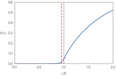
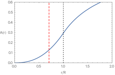
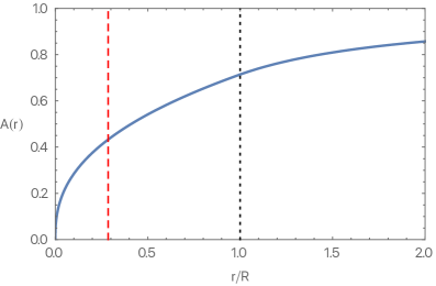
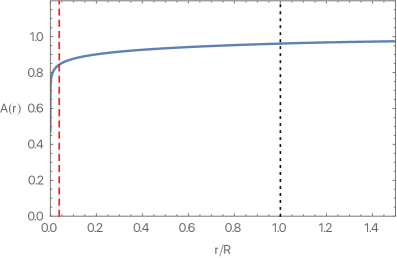
Figure 1: The time-time metric component $A(r)$ (see our metric Ansatz in eq (2.3)) both in the interior and exterior of the star. We make the following choices (from left-to-right and top-to-bottom) of the exponent $\gamma$: $\gamma=10.2,\,1.2,\,0.2,\,0.02$. Red dashed line: the Schwarzschild radius $r=2M$. Black dashed line: the position of the star surface $r=R$.

We turn off possible additional contributions associated with parameters $\sigma-1$, $\gamma$ in eq (2.13) in the exterior region of the geometry, since we find that only the Schwarzschild profile in eq (2.23) allows us to consistently satisfy the matching conditions at the sphere radius $R$. We interpret this fact as a manifestation of a no-hair condition for this set-up, so that in the spherically symmetric case the exterior geometry is only characterised by the mass $M$, while it is independent from the charge $Q_{E}$. We will learn in section 4 that the story is more complex (and interesting) when breaking spherical symmetry, since then the geometry depends on magnetic and electric charges.

The vector star compactness

We find the inequality

$$r_{\rm Schw}\equiv 2M\,=\,\frac{2\,\gamma\,R}{1+2\,\gamma}\,\leq\,R\,,$$ (2.28)

showing that the Schwarzschild radius $r_{\rm Schw}$ is inside the star radius $R$. We conclude that our configuration has no horizons. Hence the non-negative parameter $\gamma$ has a transparent physical interpretation. It controls the compactness

$${\cal C}\,\equiv\,M/R$$ (2.29)

of the object we are examining. We find

$$0\,\leq\,{\cal C}\,=\,\frac{\gamma}{1+2\gamma}\,<\,\frac{1}{2}\,.$$ (2.30)

Hence this quantity spans from $0$ for $\gamma=0$ (flat space) to $1/2$ for $\gamma=\infty$, which is the same compactness of a Schwarzschild black hole. As anticipated above, the vector star can violate the Buchdahl bound ${\cal C}\leq 4/9$, thanks to a sizeable anisotropic stress.

We represent in Fig 1 the time-time metric component $A(r)$, together with the position of the would-be Schwarzschild radius, for different choices of $\gamma$. As $\gamma$ becomes smaller and smaller, the geometry approaches flat space. In the opposite case, the larger the $\gamma$ is, the nearer the Schwarzschild radius approaches from inside the surface of the star. In the limit $\gamma\to\infty$ the interior geometry is not well defined, at least in Boyer-Lindquist coordinates, since the metric profile for $A$ becomes flatter and flatter (see Fig 1, upper left panel). However, as will discuss in what comes next, this limit can be meaningful in specific contexts and applications.

2.3 Resolving the singularity in the star interior

The singularity at the star origin $r\,=\,0$ can be resolved by switching on the parameter $\sigma$ within the interval $0\leq\sigma\leq 1$ in eqs (2.13), at least for large enough values of $\gamma$. In order to obtain a configuration with a smooth matching at the star surface, the interior geometry and vector field solutions are given by (the cumbersome expression for $\Pi(r)$ can be determined plugging the next formulas in eq (2.10)):

$$\alpha_{0}(r) = \frac{2\,Q_{I}\,R}{r}+2\sigma+\frac{2\,\left(1-\sigma\right)}{1+\gamma}\,\left(\frac{r}{R}\right)^{\gamma}\,,$$ (2.31)

$$A(r) = \sigma^{2}+\frac{2\,\sigma\,\left(1-\sigma\right)}{(1+\gamma)}\,\left(\frac{r}{R}\right)^{\gamma}+\frac{\left(1-\sigma\right)^{2}}{(1+2\gamma)}\,\left(\frac{r}{R}\right)^{2\gamma}\,,$$ (2.32)

$$B(r) = \frac{A(r)}{\left[\sigma+\left(1-\sigma\right)(r/R)^{\gamma}\right]^{2}}\,.$$ (2.33)

The exterior geometry is again given by the Schwarzschild expressions (2.23), but this time the mass and the outside vector charge are given by

$$M = \frac{(1-\sigma)\,\gamma\,(1+\gamma+\sigma\,\gamma)}{(1+\gamma)(1+2\gamma)}\,R\,,$$ (2.34)

$$Q_{\rm E} = {Q}_{I}-\frac{\gamma(1-\sigma)}{1+\gamma}\,,$$ (2.35)

in order to continuously match the interior with the exterior. This configuration is typically less compact than the one of section 2.2, since now the compactness parameter ${\cal C}$ spans between ${\cal C}=0$ for $\gamma=0$, to ${\cal C}\,=\,(1-\sigma^{2})/2$ for $\gamma\to\infty$ (recall that $0\leq\sigma\leq 1$).

The curvature invariants are now no more necessarily singular for $r\to 0$. In fact, computing for example the Ricci scalar by means of eq (2.11) we find

$$\hskip-17.07182pt{\text{Ricci scalar}}\,=\,\frac{2\,r^{\gamma-2}\,\gamma\,(1-\sigma)}{\left[\sigma+(1-\sigma)\,r^{\gamma}\right]^{3}}\,\left[\sigma^{2}+\frac{\sigma\,(2-\gamma)\,(1-\sigma)}{1+\gamma}\,r^{\gamma}+\frac{(1-\gamma)\,(1-\sigma)^{2}}{1+2\gamma}\,r^{2\gamma}\right]\,.$$ (2.36)

Hence, if $\gamma\geq 2$, the Ricci scalar can be non-singular at the origin, when turning on any positive value for $\sigma$. The other curvature invariants built in terms of the Riemann and Ricci tensors show a similar behaviour.

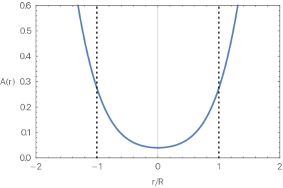
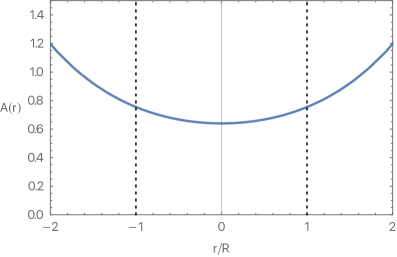
Figure 2: The time-time metric profile $A(r)$ of eq (2.32) evaluated nearby the origin, choosing $\gamma=2$ and $\sigma=0.2$ (left panel) and $\sigma=0.8$ (right panel).

We represent in Fig 2 the profile for $A(r)$, which makes manifest that this function is non-vanishing at the origin and can be continued for negative $r$. One might explore these configurations as possible wormhole solutions [55, 56], and study their properties and their stability. Notice that the parameter $\sigma$ here is free in the interval $0\,\leq\,\sigma\,\leq\,1$: it would be interesting to determine physical motivations for its size and how to relate it with observable properties, as for some wormhole configurations [57]. We postpone these questions to future work.

3 Geodesics

We learned in the previous section that – when considering spherically symmetric configurations – the exterior geometry of our vector star solutions corresponds to a Schwarzschild space-time. In this and the next section we discuss possible methods for distinguishing our system from GR configurations, and for probing the interior properties of the star.

We start studying time-like and null-like geodesics, as a probe of the internal geometry of the star. The behaviour of geodesics around our configuration can be richer  than what occurs in a Schwarzschild geometry within GR, also thanks to the possibility of having geodesics crossing the star surface in both directions, probing its interior.

In fact, the analytic study of geodesics is important for understanding the global and causal properties of the geometry under consideration. For time-like geodesics, we show that there can be additional stable circular orbits with respect to Schwarzschild black holes. Geodesics can cross the star surface in both directions, probing its compactness. For null-like geodesics, we study the connections between the compactness of the configuration, and the existence of unstable circular orbits, the light rings associated with a photosphere [51]. We assume that the probe particle experiencing the geometry is uncharged under the vector field $V_{\mu}$.

We explore the case $\sigma=0$ and focus on the configurations of section 2.2. Using standard textbook methods it is straightforward to obtain the relevant geodesic equations. We study the trajectory of a probe particle at radial position $r(\tau)$, with $\tau$ indicating the particle proper time. We introduce the dimensionless combination

$$y(\tau)\,\equiv\,\frac{r(\tau)}{R}\,,$$ (3.1)

with $R$ indicating the radius of the star.

For the case of time-like geodesics, when $y>1$ the particle is outside the star, and experiences a Schwarzschild space-time characterised by a mass $M$ related with $\gamma$ by eq (2.27). The particle geodesics is controlled by the equation

$$\frac{1}{2}\left(\frac{dy}{d\tau}\right)^{2}+U_{\rm ext}(y)\,=\,\frac{\cal E}{R^{2}}\,\,\,,\hskip 28.45274pt{\text{for $y\geq 1$.}}$$ (3.2)

The geodesic potential is

$$U_{\rm ext}(y) = \frac{1}{R^{2}}\,\left[-\frac{M}{R\,y}+\frac{\ell^{2}}{2\,y^{2}}-\frac{M\,\ell^{2}}{R\,y^{3}}\right]\,,$$ (3.3)

$$= \frac{1}{(1+2\gamma)\,R^{2}}\,\left[-\frac{\gamma}{y}+\frac{\ell^{2}\,(1+2\gamma)}{2\,y^{2}}-\frac{\gamma\,\ell^{2}}{y^{3}}\right]\,.$$

In eqs (3.2)-(3.3) the quantity ${\cal E}$ is a parameter associated with the conserved energy of the probe particle, and $\ell\,=\,L/R$ is a convenient dimensionless combination, with $L$ indicating the conserved angular momentum of the particle.

The particle trajectory in the interior of the star, $y\leq 1$, is instead described by the equation

$$\frac{1}{2}\left(\frac{dy}{d\tau}\right)^{2}+U_{\rm int}(y)\,=\,\frac{\cal E}{R^{2}}\,\,,\hskip 28.45274pt{\text{for $y\leq 1$.}}$$ (3.4)

The interior potential is

$$U_{\rm int}(y) = \frac{\left(1+\gamma\right)^{2}}{2\,R^{2}\,(1+2\gamma)}\times$$ (3.5)

$$\hskip-8.5359pt\,\left[y^{\frac{2\gamma}{(1+\gamma)}}+\left(\frac{\ell^{2}}{\left(1+\gamma\right)}+\frac{\gamma^{2}}{1-\gamma^{2}}\right)\,{y^{-\frac{2(1-\gamma)}{1+\gamma}}}-\frac{1+\gamma\left(3+\ell^{2}-\gamma(2+\ell^{2})\right)}{\left(1-\gamma^{2}\right)\,\left(1+\gamma\right)}\right]\,.$$

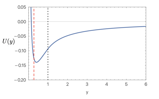
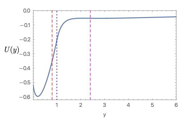
Figure 3: Particle potential for time-like geodesics. Left panel: $\gamma=\ell=1/8$. Right panel $\gamma=2$, $\ell=1.4$. Black dashed line: star surface. Red dashed line: Schwarzschild radius. On the right we include in magenta dashed line the innermost stable circular orbit position calculated within GR, and located at $y\,=\,6\,M\,R$. Both panels makes manifest that there are extrema of the geodesic potential located within the star radius.

The integration constants characterising the interior potential (3.5) have been chosen so to ensure that the potential $U_{\rm int}(y)$, together with its first derivative , is continuously connected with the potential $U_{\rm ext}(y)$ at the star surface $y=1$. When $\gamma<1$ the interior potential is unbounded and diverges at plus infinity at the origin. This implies that a time-like geodesics entering the star can not reach the singularity, and bounces back to the exterior (more on this later). We represent in Fig 3 the entire profile of the geodesic time-like potential, for two representative values of $\gamma$.

We can now study more quantitatively the main features of time-like geodesics, using our expressions (3.3) and (3.5) for the potentials. In the exterior part of the geometry $y\geq 1$ (or $r\geq R$), the potential has extrema if the following condition is realised

$$\ell\,>\,\sqrt{12}\,\frac{\gamma}{1+2\gamma}\,.$$ (3.6)

When this inequality is satisfied, the extrema are located at the positions

$$y_{0}\,=\,\frac{\ell^{2}\,(1+2\gamma)}{2\,\gamma}\left[1\,\pm\,\sqrt{1-\frac{12\gamma^{2}}{\ell^{2}(1+2\gamma)^{2}}}\right]\,.$$ (3.7)

The plus choice corresponds a maximum of the potential (always located in the star exterior), the minus choice is a minimum of the potential. The innermost stable circular orbit (ISCO) in the star exterior is at

$$y_{\rm isco}\,=\,\frac{6\gamma}{1+2\,\gamma}\,,$$ (3.8)

and is outside the star if we choose $\gamma>1/4$.

Considering now the interior geometry, we find that the potential (3.5) admits an extremal point at

$$y_{0}^{\frac{2}{1+\gamma}}\,=\,\frac{\gamma^{2}+(1-\gamma)\,\ell^{2}}{\gamma(1+\gamma)}\,.$$ (3.9)

The position $y_{0}$ lies within the star interior if the following condition on $\ell$ is satisfied

$$\ell^{2} < \frac{\gamma}{1-\gamma}\hskip 28.45274pt{\text{for $\gamma<1$}}\,,$$ (3.10)

$$\ell^{2} < \frac{\gamma^{2}}{\gamma-1}\hskip 28.45274pt{\text{for $\gamma>1$}}\,.$$ (3.11)

The value $\gamma=1$ is special case, since the extremum is always at $y=1/2$ (regardless of the value of $\ell$). When $\gamma>1/4$, by tuning $\ell$, we can have local stable minima for the time-like geodesic potential both in the star interior and the star exterior, as shown in Figure 3 (right panel).

It is interesting to study time-like geodesics which cross the star surface in both directions: we can use them for probing the star interior. In this case, the analysis of the particle trajectories can help in determining the properties of the internal geometry. The simplest option are radial plunge orbits, that start at rest from plus infinity with zero angular momentum, and enter inside the star radius. Let us then choose ${\cal E}=\ell=0$ in the geodesic evolution equations. If we further choose $\gamma<1$, the interior potential (see eq (3.5)) has an infinite barrier at the origin, which prevents the trajectory from falling into the singularity. A massive particle arriving from infinitely far away enters into the star region with finite velocity at the star radius, and changes the direction of its speed at the zero of the internal potential $U_{\rm int}$. Then it bounces, crossing the star surface with the same velocity (in opposite direction) as it enters, and then travels back to infinite distance from the star. In such a situation, the propert time $\tau_{\rm int}$ spent within the star in the ‘bouncing process’ depends only on $\gamma$, and on the star radius. An observer far away from the star, who measures the time for radial plunge orbits to reach the star and bounce back, can then infer the star compactness.

The proper time $\tau_{\rm int}$ spent within the star interior is given by the integral

$$\frac{\tau_{\rm int}(\gamma,R)}{R} = \frac{\sqrt{2}}{R}\,\int_{y_{\star}}^{1}\,\frac{dy}{\sqrt{-U_{\rm int}(y)}}\,,$$ (3.12)

$$= \frac{\sqrt{4+8\gamma}}{1+\gamma}\,\int_{y_{\star}}^{1}\,\frac{dy}{y^{\frac{\gamma-1}{\gamma+1}}}\,\left[\frac{\left(1+3\gamma-2\gamma^{2}\right)\,y^{\frac{2(1-\gamma)}{(1+\gamma)}}}{(1-\gamma)(1+\gamma)^{2}}-y^{\frac{2}{(1+\gamma)}}-\frac{\gamma^{2}}{1-\gamma^{2}}\right]^{-1/2}\,,$$ (3.13)

where $y_{\star}$ is the zero of the potential in the interior – i.e. the zero of the integrand function within square parenthesis in eq (3.13). In general, this expression needs to be integrated numerically, although for some special values of $\gamma$ an analytical integration is possible.

For example, for $\gamma=1/2$ we get

$$T_{\rm int}(1/2,R) = -\frac{4\,\sqrt{2}}{3}\,\left(1+\frac{4}{3}\,\arccos\left[-\frac{1}{\sqrt{37}}\right]\right)\,R\,,$$ (3.14)

$$\simeq 2.48\,R\,.$$ (3.15)

Given its dependence on the value of $\gamma$, the time spent by a particle travelling along the geodesics in the interior geometry of the star configuration can be used as a tool for studying the star properties, as its compactness that depends on $\gamma$ and $R$ through relation (2.30).

The equation for null-like geodesics results

$$\frac{1}{2}y^{\prime 2}+\frac{1}{R^{2}}\,\frac{\ell^{2}}{2\,y^{2}}\left(1-\frac{2\gamma}{(1+2\gamma)\,y}\right)\,=\,\frac{{\cal E}^{2}}{R^{2}}\,,$$ (3.16)

in the exterior. (The various quantities have the same meanings as in the previous time-like case.) Imposing continuity of the function $y(\tau)$ and its first derivatives at the star surface, we find the following equation for null-like geodesics in the interior

$$\frac{1}{2}y^{\prime 2}+\frac{1}{R^{2}}\,\frac{\ell^{2}}{2\,(1+2\gamma)}\left(-\gamma+(1+\gamma)\,y^{-\frac{2(1-\gamma)}{(1+\gamma)}}\right)\,=\,\frac{{\cal E}^{2}}{R^{2}}\,.$$ (3.17)

These results indicate that the interior geometry has no extremal points for null-like geodesics. The exterior potential admits one maximum at

$$y_{\rm ext}\,=\,\frac{3\gamma}{1+2\gamma}$$ (3.18)

If $\gamma>1$, $y_{\rm ext}$ is located in the exterior region of the star. Hence, if this condition is satisfied, the null-like geodesic potential have a maximum which can be associated with a light-ring and the photosphere: the situation is then very similar to GR. For $\gamma<1$ there is no local maximum instead, and there instead is an infinite barrier for light rays: the situation is then similar to what we discussed in the case of time-like geodesics. The value $\gamma=1$ is special because the potential is constant. The condition for having a photosphere, $\gamma>1$, corresponds to the condition of considering ultracompact objects, ${\cal C}>1/3$, in agreement with the general analysis of [51].

4 Beyond spherical symmetry

We have seen that the behaviour of geodesics can be richer with respect to what occurs in a Schwarzschild geometry, since geodesics can probe the star interior. In this section we go beyond spherical symmetry, considering the dynamics of fluctuations of the vector field and of the metric tensor, both outside and inside the star. We will learn that their properties are sensitive to vector charges (both electric and magnetic-type ones) as well as the star compactness. They can then offer probes for distinguishing a vector star from a black hole, as well as to investigate applications of no-hair arguments in this context.

We focus on parity-odd, spin-1 stationary fluctuations: they are easier to deal with analytically, and can lead to distinctive effects in systems (like ours) with a pronounced anisotropic stress in the internal stress-tensor of the star. Our aims are as follows:

1. First, in section 4.1 we analytically investigate the response of the vector-field profile $V_{\mu}$ to magnetic-type, spin-1 perturbations, which add magnetic-type charges to the vector star solution. We determine the structure of the dipolar magnetic field which can be sourced by the star configuration, as well as the vector magnetic susceptibility to the application of an external field. The characteristic response of the vector can be used as a probe of the star properties, playing a role analog to neutron star Love numbers [58, 59, 60] for distinguishing exotic compact objects from black holes [61].

2. Then, in section 4.2 we focus on metric fluctuations, and study the behaviour of the corresponding parity-odd spin-1 deformations. They break spherical symmetry, and can be sourced by magnetic-type deformations of the vector profile studied in section 4.1. Their properties depend on the electric and magnetic charges, showing that – when breaking spherical symmetry – the exterior geometry becomes sensitive to the properties of the vector configuration. We are also able to characterize the properties of fluctuations in the interior of the star, and their dependence on the vector charge.

4.1 Magnetic charge, and the vector magnetic susceptibility

We start studying the dynamics of parity-odd, magnetic fluctuations of the vector field profile $V_{\mu}$, that contribute to the total combination

$$V_{\mu}\,dx^{\mu}+\delta V_{\mu}\,dx^{\mu}\,,$$ (4.1)

defining the total vector field background$+$fluctuations. We focus on this section on the vector fluctuations $\delta V_{\mu}$ only: we study their backreaction on the metric in section 4.2. The first part of eq (4.1), $V_{\mu}\,dx^{\mu}$, contains the background electric-type components, as in eq (2.4). Its profile in the internal and external regions of space-time are given in eqs (2.16) and (2.24) (we focus on the case of singular internal geometry of section 2.2). On top, we have the second contribution to eq (4.1). Parity-odd, spin-1 stationary fluctuations are parameterised by

$$\delta V_{\mu}\,dx^{\mu}\,\equiv\,\,\frac{a_{\varphi}(r)}{\sin\theta}\,\left(\partial_{\varphi}Y_{\ell m}(\theta,\varphi)\right)\,d\theta-\,{a_{\varphi}(r)}\,{\sin\theta}\,\left(\partial_{\theta}Y_{\ell m}(\theta,\varphi)\right)\,d\varphi\,,$$ (4.2)

in terms of a function $a_{\varphi}(r)$. In this formula the $Y_{\ell m}$ are the scalar spherical harmonics, and their gradients are associated with the spin-1 spherical harmonics (see e.g. [62, 63]) we are interested in. They are characterised by a multipole index $\ell$ ($\ell\geq 1$) and an azymuthal index $m$: in our study of fluctuations around spherically symmetric configurations, there is no dependence on the index $m$ hence we understand it from now on. We assume that the quantities $a_{\varphi}(r)$ are small. We obtain the linearised equations in the exterior ($r\geq R$) and interior $(r\leq R)$ of the star as

$$0 = a_{\varphi}^{\prime\prime}+\frac{2Q_{E}\,R}{r(Q_{E}\,R+r)}\,a_{\varphi}^{\prime}-\frac{2Q_{E}R+\ell(\ell+1)\,r}{r(Q_{E}\,R+r)^{2}}\,a_{\varphi}\,=\,0\hskip 28.45274pt,\,\,$$ (4.3)

$$0 = a_{\varphi}^{\prime\prime}+\frac{Q_{I}(2+\gamma-\gamma^{2})-3\gamma(r/R)^{1+\gamma}}{r\left(Q_{I}(1+\gamma)+(r/R)^{1+\gamma}\right)}\,a_{\varphi}^{\prime}+$$

$$+ \hskip-2.84544pt\frac{2\,Q_{I}^{2}\,\gamma\,\left(1+\gamma\right)+Q_{I}(r/R)^{1+\gamma}\left(1+\gamma\right)\left(1+2\gamma\right)-2(r/R)^{2+2\gamma}\left(\ell+\gamma(\ell-1)\right)\left(1+\ell+(\ell+2)\gamma\right)}{2\,r^{2}\left(Q_{I}(1+\gamma)+(r/R)^{1+\gamma}\right)^{2}}\,a_{\varphi}$$

The internal electric charge $Q_{I}$ is related with the external one $Q_{E}$ by the relation (2.26). Interestingly, in both the exterior and interior regions the equations governing the vector fluctuations $a_{\varphi}$ are decoupled from the parity-odd metric perturbations . However, as we will learn, the vector modes $a_{\varphi}$ backreact on the metric at the linearised level, breaking spherical symmetry. Notice that also the exterior equation (4.3) depends on the star electric charge, indicating that the behaviour of the external magnetic deformation is controlled by $Q_{E}$.

The two equations (4.3) and (4.1) admit two distinct exact solutions, each depending on two integration constants. Fixing the integration constants in the interior so that the solutions continuously match – together with their derivative – at the star surface $r\,=\,R$, we get

$$a_{\varphi}(r) = \frac{P_{\varphi}\,R}{r}\,\left(Q_{E}+r/R\right)^{1-\ell}+\frac{S_{\varphi}\,R}{r}\,\left(Q_{E}+r/R\right)^{2+\ell}\,,$$ (4.5)

$$a_{\varphi}(r) = \frac{P_{\varphi}\,R}{r}\,\left(\frac{Q_{E}(1+\gamma)+\gamma+(r/R)^{1+\gamma}}{1+\gamma}\right)^{1-\ell}$$ (4.6)

$$+\frac{S_{\varphi}\,R}{r}\,\left(\frac{Q_{E}(1+\gamma)+\gamma+(r/R)^{1+\gamma}}{1+\gamma}\right)^{2+\ell}\,,$$

for two constants $P_{\varphi}$, $S_{\varphi}$, respectively in the exterior – eq (4.5) – and in the interior – eq (4.6) – of the star configuration.

We now study two applications of the previous general solutions. In the first case, we interpret the solutions (4.5)-(4.6) as controlling a magnetic dipolar potential of the star configuration, with a magnetic field strength decaying at infinity. Hence, we select $\ell=1$ and $S_{\varphi}\,=\,0$: the vector potential component $\delta V_{\varphi}$ becomes

$$\delta V_{\varphi} = -a_{\varphi}(r)\,\sin\theta\,\left(\partial_{\theta}Y_{10}(\theta)\right)\,,$$ (4.7)

$$= \sqrt{\frac{3}{4\pi}}\,P_{\varphi}\,\frac{R}{r}\,\sin^{2}\theta\,,$$

for any $r>0$. This leads to a dipolar, parity-odd magnetic field deformation $B_{\hat{r}}$ along the radial direction, which can be computed through the vector field strength using standard formulas

$$B_{\hat{r}}\,=\,\frac{\partial_{\theta}\,V_{\varphi}}{r^{2}\,\sin\theta}\,=\,P_{\varphi}\,\sqrt{\frac{3}{\pi}}\,\frac{R}{r^{3}}\,\cos\theta\,.$$ (4.8)

The dipolar magnetic field of the star is then controlled by the magnetic dipolar charge $P_{\varphi}$.

In the second case, we study the response of the system to an external constant dipolar magnetic field, whose radial component behaves at large distances ($r\to\infty$) as

$$B_{\hat{r}}^{\rm(ext)}(r\to\infty)\,=\,C_{0}\,\cos\theta\hskip 14.22636pt\Rightarrow\hskip 14.22636pta_{\varphi}^{\rm(ext)}(r\to\infty)\,=\,C_{0}\,\sqrt{\frac{\pi}{3}}\,r^{2}\,,$$ (4.9)

for a small constant $C_{0}$. In passing from the left to the right of the arrow in eq (4.9), we made use of the definitions in eqs (4.7)-(4.8).

In studying the star vector response to the external field (4.9) – a phenomenon that we call vector magnetic susceptibility – we impose for definiteness that the magnetic-type fluctuations $a_{\varphi}$ do not blow-up at the origin $r=0$, so to fix the last of the integration constants in eq (4.6). The regularity condition requires that $P_{\varphi}$ and $S_{\varphi}$ in eq (4.6) are related by the condition

$$\frac{S_{\varphi}}{P_{\varphi}}\,=\,-\frac{\left(1+\gamma\right)^{1+2\ell}}{\left(Q_{E}(1+\gamma)+\gamma\right)^{1+2\ell}}\,.$$ (4.10)

Requiring to match the asymptotic value of the magnetic field as in eq (4.9), we fix the last of the integration constants, and find the following solution for $a_{\varphi}$:

$$a_{\varphi}(r) = C_{0}\,\sqrt{\frac{\pi}{3}}\,\frac{R^{3}}{r}\,\left(Q_{E}+r/R\right)^{3}\left[1-\left(\frac{R}{r}\right)^{3}\frac{\left(Q_{E}+\gamma/(1+\gamma)\right)^{3}}{\left(Q_{E}\,R/r+1\right)^{3}}\,\right]\,.$$ (4.11)

While the part outside the squared parenthesis matches the boundary condition at spatial infinity, the part inside the parenthesis controls to the dipolar susceptibility of the external magnetic field. Interestingly, such vector magnetic susceptibility depends both on the electric charge $Q_{E}$ and the parameter $\gamma$ controlling the star compactness. This quantity is analogous, although not identical, to the gravitational magnetic susceptibility as studied in various works in the context of studies of tidal deformability for black holes – see e.g. [64, 65, 66, 63].

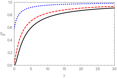
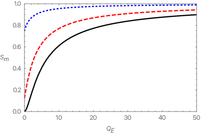
Figure 4: Plots of the vector magnetic susceptibility of eq (4.12), as function of $\gamma$ (left panel) and $Q_{E}$ (right panel). Left: $Q_{E}=1/10$ (black); $Q_{E}=1$ (red dashed); $Q_{E}=10$ (blue dotted). Right: $\gamma=1/10$ (black); $\gamma=1$ (red dashed); $\gamma=10$ (blue dotted).

Defining the vector magnetic susceptibility ${\cal S}_{m}$ as the opposite of the second term in the squared parenthesis of eq (4.11), evaluated at the star surface $r=R$, we get

$${\cal S}_{m}\equiv\frac{\left(Q_{E}+\gamma/(1+\gamma)\right)^{3}}{\left(Q_{E}\,+1\right)^{3}}\,.$$ (4.12)

Interestingly, this quantity approaches the value ${\cal S}_{m}=1$ for very large $\gamma$, showing that in the limit of ultracompact objects approaching the compactness of a black hole, the susceptibility behaves as the one of a conducting sphere.

We plot in Fig 4 examples of the dependence of ${\cal S}_{m}$ on $Q_{E}$ and $\gamma$, for some representative cases. It would be interesting to find measurable observables sensitive to the value of ${\cal S}_{m}$, which can represent distinctive probes of the properties of the star – its charges and compactness.

4.2 Parity-odd stationary deformations of the metric, and star rotation

After discussing the perturbations in the vector field, we now focus on parity-odd, stationary fluctuations of the metric, along the lines of the classical analysis of [67]. To slightly reduce the length of our formulas, in this section we set the star radius $R=1$.

We decompose the metric in a background part and perturbations:

$$g_{\mu\nu}dx^{\mu}dx^{\nu}+h_{\mu\nu}dx^{\mu}dx^{\nu}\,.$$ (4.13)

In this equation, $g_{\mu\nu}dx^{\mu}dx^{\nu}$ corresponds to the spherically symmetric background solution with Ansatz (2.3), with exterior and interior metric components studied in section 2. The quantity $h_{\mu\nu}dx^{\mu}dx^{\nu}$ controls the parity-odd, spin-1 stationary metric fluctuations in Regge-Wheeler gauge:

$$\small{h_{\mu\nu}=\begin{pmatrix}0&0&-h_{0}(r)\sin\theta^{-1}\,\partial_{\varphi}&h_{0}(r)\sin\theta\,\partial_{\theta}\\ 0&0&-h_{1}(r)\sin\theta^{-1}\,\partial_{\varphi}&h_{1}(r)\sin\theta\,\partial_{\theta}\\ -h_{0}(r)\sin\theta^{-1}\,\partial_{\varphi}&-h_{1}(r)\sin\theta^{-1}\,\partial_{\varphi}&0&0\\ h_{0}(r)\sin\theta\,\partial_{\theta}&h_{1}(r)\sin\theta\,\partial_{\theta}&0&0\\ \end{pmatrix}}Y(\theta,\varphi).$$ (4.14)

The metric fluctuations break the spherical symmetry of the system. The angular dependence of the solution is controlled by derivatives of the scalar spherical harmonics $Y_{\ell m}(\theta,\varphi)$ ($\ell\geq 1$) which define spin-1 spherical harmonics as in the previous section. It is straightforward to determine the expression for the linearized equations controlling the radial profiles of the metric components $h_{0}(r)$ and $h_{1}(r)$, and how they are sourced by the magnetic-type vector fluctuations studied in section 4.1. For the case $\ell=1$, the function $h_{1}(r)$ is a gauge mode and can be set to zero; for $\ell\geq 2$, the equation of $h_{1}$ is algebraic, and can be solved as a function of $h_{0}$ and $a_{\varphi}$, both in the exterior and the interior of the star. For example, in the star exterior we find

$$h_{1}(r)\,=\,\frac{r}{r-2M}\,\frac{\sqrt{Q_{E}^{2}+2Mr+Q_{E}r}}{Q_{E}+r}\,h_{0}(r)-\frac{r\,\sqrt{Q_{E}^{2}+2\,M\,r+Q_{E}\,r}}{2(Q_{E}+r)^{2}}\,a_{\varphi}(r)\,.$$ (4.15)

Plugging this expression into the equation for $a_{\varphi}$ we find equation (4.3), that – as explained in section 4.1 – is decoupled from metric fluctuations. The quantity $h_{0}(r)$ is controlled by the following equation in the star exterior, valid for any $\ell\geq 1$ (we understand the dependence on $r$):

$$0 = h_{0}^{\prime\prime}-\frac{4Q_{E}}{r\,(Q_{E}+r)}\,h_{0}^{\prime}+\frac{\left(6Q_{E}^{2}+4\,Q_{E}\,r-\ell(\ell+1)r^{2}\right)}{r^{2}\,\left(Q_{E}+r\right)^{2}}\,h_{0}+\frac{4M-2r}{Q_{E}+r}\,a_{\varphi}^{\prime\prime}-\frac{4M}{r}\,\frac{a_{\varphi}^{\prime}}{Q_{E}+r}$$

$$+ \frac{a_{\varphi}}{r\,(Q_{E}+r)^{3}}\left[Q_{E}^{2}\left(1+\frac{3}{2}\ell(\ell+1)\right)+2Mr+\left(1+\frac{3}{2}\ell(\ell+1)\right)Q_{E}r-\ell(\ell+1)(M-2r)\,r\right]\,.$$

Notice that the metric component $h_{0}(r)$ is sourced by the magnetic-type vector perturbation $a_{\varphi}(r)$. The equation for $h_{0}$ in the star interior can also be derived quite easily, but is longer and we do not write it explicitly.

Let us study explicit examples of solutions. Focus on the dipolar case $\ell=1$, $m=0$ (and $h_{1}=0$), and on perturbations that decay at infinity. As first noticed in [67], the metric then describes a slowly rotating configuration, with $h_{0}(r)$ controlling the stationary rotation of the geometry through an off-diagonal metric component

$$g_{t\varphi}\,dt\,d\varphi\,=\,-2\,\left(\sqrt{\frac{3}{4\pi}}\,\frac{h_{0}(r)}{r^{2}}\right)\,r^{2}\,\sin^{2}\theta\,dt\,d\varphi\,.$$ (4.17)

It is straightforward to solve eq (LABEL:eqh0stext) for $h_{0}(r)$ in the star exterior, taking as source the magnetic-type solution we found in eq (4.5) with $\ell=1$ and $S_{\varphi}=0$. We find for $r\geq 1$

$$-\sqrt{\frac{3}{4\pi}}\,\frac{h_{0}(r)}{r^{2}}\,=\,\frac{a\,M}{(Q_{E}+r)^{3}}+\sqrt{\frac{3}{\pi}}\,\frac{P_{\varphi}\,M}{Q_{E}\,r^{3}}\,,$$ (4.18)

with $a$ an integration constant associated with the rotation of the geometry (the Kerr parameter), and $P_{\varphi}$ the intrinsic magnetic dipolar charge as given in eq (4.7) above. This metric coefficient should be compared with the one found in the slowly-rotating limit of the Kerr solution in GR:

$$-\sqrt{\frac{3}{4\pi}}\,\frac{h^{\rm GR}_{0}(r)}{r^{2}}\,=\,\frac{a\,M}{r^{3}}\,.$$ (4.19)

Comparing (4.18) with (4.19), we find that the magnetic charges $P_{\varphi}$ and $Q_{E}$ influence the geometry as vector hairs, and contribute in breaking the spherical symmetry of the configuration to an axial one. Interestingly, $Q_{E}$ appears at the denominators: we interpret this fact as a consequence of the specific non-minimal couplings of the vector to gravity. The quantity $Q_{E}$ contributes to modulate the $1/r^{3}$ decay at large distances of the angular momentum contribution proportional to $a$. Instead, $P_{\varphi}/Q_{E}$ adds a new contribution to $h_{0}$, absent in the vacuum GR case, being induced by the magnetic dipolar charge of the star configuration.

The peculiar dependence on the radial coordinate $r$ in eq (4.18) can lead to interesting effects, distinctive of the vector-tensor system under consideration. Let us suppose that $a$ and $P_{\varphi}$ have opposite sign (say $a$ is positive) and call

$$\nu^{3}\,\equiv\,-\sqrt{{3}/{\pi}}\,{|P_{\varphi}|\,M}/{(Q_{E}\,a)}$$ (4.20)

We assume $0\,\leq\,\nu\,<\,1$. We can rewrite eq (4.18) as

$$-\sqrt{\frac{3}{4\pi}}\,\frac{h_{0}(r)}{r^{2}}\,=\,\frac{a\,M}{r^{3}}\left(\frac{r^{3}}{(Q_{E}+r)^{3}}-{\nu^{3}}\right)\,.$$ (4.21)

While for large values of $r$ the right hand side of (4.21) is positive, as we approach the star the sign of $h_{0}(r)$ changes. This occurs at

$$r_{\star}\,=\,\frac{\nu\,Q_{E}}{1-\nu}$$ (4.22)

which is larger than the star radius $R=1$ by choosing a large enough $Q_{E}$. This fact implies that the direction of rotation of the space-time changes as we approach the star, due to to the opposite contributions to rotation of the Kerr parameter $a$ and the magnetic charge $P_{\varphi}$. It would be interesting to further explore the consequences of this phenomenon, and whether can be used to find distinctive probes of this system.

The discussion of the interior part of the geometry is particularly simple in the case $P_{\varphi}\,=\,0$: let us focus for simplicity on this case for the rest of the section, although analytic expressions for $P_{\varphi}\,\neq\,0$ can also be found. This limit implies that the exterior dipolar configuration is described by eq (4.18) with no magnetic-charge contribution. The interior solution $r\leq 1$ of the field equations for $h_{0}$ that continuously match with the exterior for $r\geq 1$ is

$$-\sqrt{\frac{3}{4\pi}}\,\frac{h_{0}(r)}{r^{2}} = \frac{a\,M\,(1+\gamma)^{3}}{\left[Q_{E}(1+\gamma)+\gamma(1-\sigma)+\,r^{1+\gamma}(1-\sigma)+\,r\,\sigma\,(1+\gamma)\right]^{3}}\,,$$ (4.23)

where we selected as interior background configuration the solution described in section 2.3. The interior part of the star is dragged by the rotation of the configuration: the dragging effects are also modulated by the electric charge $Q_{E}$ and depend on the star compactness through the parameter $\gamma$. While in this example we focussed on the case $\ell=1$, the cases $\ell\geq 2$ can also be straightforwardly analysed, at least in absence of intrinsic magnetic charge, and the previous formulas generalise by changing the exponents from $3$ to $\ell+2$.

In summary, the study of properties of parity-odd stationary metric fluctuations reveal a very rich structure that goes beyond what found in solutions of GR in empty space, even if the exterior star geometry is given by Schwarzschild space-time. Both the exterior and the interior metric elements are indeed sensitive to the vector properties. A detailed analysis of time-dependent perturbations, as well as parity-even modes, is left for future studies.

5 Outlook

In this work we presented and investigated new analytic solutions describing a family of horizonless compact objects in vector-tensor theories of gravity, dubbed ultracompact vector stars. They are sourced by a vector condensate, induced by a non-minimal coupling with gravity. They can be as compact as black holes, thanks to their internal anisotropic stress. In the spherically symmetric case, their external geometry corresponds to the Schwarzschild solution as in GR, even if they can be characterised by an electric-type charge. The interior part of the solution resembles a singular isothermal sphere, and the singularity at the star centre can be resolved by tuning some of the available integration constants. The interior configuration is smoothly matched to the exterior geometry of the star, with no need of extra stress-tensor on the star surface.

We investigated features of our systems that allow one to distinguish vector star objects from GR black hole solutions. We analytically studied the behaviour of geodesics trajectories within the star interior – where new stable circular orbits are allowed – as well as geodesics crossing in both ways the star surface. We analytically investigated parity-odd stationary fluctuations that break spherical symmetry and can assign a magnetic charge to our vector star configurations.

It would be interesting to further develop our analysis along the following directions:

• Study time-dependent fluctuations – both odd and even parity – and investigate the stability the horizonless vector star objects. This topic is particularly interesting since black hole configurations in vector-tensor theories of gravity have been shown to have instabilities [68, 69] which might be cured (or not) in more general configurations like ours.

• Study mechanisms of formation of vector stars from a process of gravitational collapse, including further sources of energy momentum tensor in the form of standard matter. Gravitationally bound solitons made of dark-matter vector bosons – in a Proca theory – have been recently numerically investigated in [70, 71, 72, 73], and would be interesting to pursue similar studies in our context. In fact, non-minimal couplings of the vector with gravity are allowed (and expected) once the vector Abelian symmetry is broken.

• Determine solutions with a large rotation parameter in the exterior geometry – the analog of Kerr – and large magnetic charge. Investigate the properties and phenomenology of the resulting magnetically-charged configurations, for example taking inspiration from [74].

• Determine additional field-theory and cosmological motivations for the vector-tensor theories we consider and their possible extensions for dark matter and dark energy.

We leave these points to future investigations.

References

- [1] J. D. Bekenstein, “Black hole hair: 25 - years after,” in 2nd International Sakharov Conference on Physics, pp. 216–219. 5, 1996. arXiv:gr-qc/9605059.
- [2] R. M. Wald, “Gravitational collapse and cosmic censorship,” pp. 69–85. 10, 1997. arXiv:gr-qc/9710068.
- [3] S. L. Shapiro and S. A. Teukolsky, Black holes, white dwarfs, and neutron stars: The physics of compact objects. 1983.
- [4] N. Yunes, K. Yagi, and F. Pretorius, “Theoretical Physics Implications of the Binary Black-Hole Mergers GW150914 and GW151226,” Phys. Rev. D 94 no. 8, (2016) 084002, arXiv:1603.08955 [gr-qc].
- [5] L. Barack et al., “Black holes, gravitational waves and fundamental physics: a roadmap,” Class. Quant. Grav. 36 no. 14, (2019) 143001, arXiv:1806.05195 [gr-qc].
- [6] D. J. Kaup, “Klein-Gordon Geon,” Phys. Rev. 172 (1968) 1331–1342.
- [7] D. A. Feinblum and W. A. McKinley, “Stable States of a Scalar Particle in Its Own Gravitational Field,” Phys. Rev. 168 no. 5, (1968) 1445.
- [8] R. Ruffini and S. Bonazzola, “Systems of selfgravitating particles in general relativity and the concept of an equation of state,” Phys. Rev. 187 (1969) 1767–1783.
- [9] S. L. Liebling and C. Palenzuela, “Dynamical Boson Stars,” Living Rev. Rel. 15 (2012) 6, arXiv:1202.5809 [gr-qc].
- [10] L. Visinelli, “Boson stars and oscillatons: A review,” Int. J. Mod. Phys. D 30 no. 15, (2021) 2130006, arXiv:2109.05481 [gr-qc].
- [11] R. Brito, V. Cardoso, C. A. R. Herdeiro, and E. Radu, “Proca stars: Gravitating Bose–Einstein condensates of massive spin 1 particles,” Phys. Lett. B 752 (2016) 291–295, arXiv:1508.05395 [gr-qc].
- [12] I. Salazar Landea and F. García, “Charged Proca Stars,” Phys. Rev. D 94 no. 10, (2016) 104006, arXiv:1608.00011 [hep-th].
- [13] M. Minamitsuji, “Proca stars with nonminimal coupling to the Einstein tensor,” Phys. Rev. D 96 no. 4, (2017) 044017, arXiv:1708.05358 [gr-qc].
- [14] P. O. Mazur and E. Mottola, “Gravitational condensate stars: An alternative to black holes,” arXiv:gr-qc/0109035.
- [15] P. O. Mazur and E. Mottola, “Surface tension and negative pressure interior of a non-singular ‘black hole’,” Class. Quant. Grav. 32 no. 21, (2015) 215024, arXiv:1501.03806 [gr-qc].
- [16] C. Cattoen, T. Faber, and M. Visser, “Gravastars must have anisotropic pressures,” Class. Quant. Grav. 22 (2005) 4189–4202, arXiv:gr-qc/0505137.
- [17] C. B. M. H. Chirenti and L. Rezzolla, “How to tell a gravastar from a black hole,” Class. Quant. Grav. 24 (2007) 4191–4206, arXiv:0706.1513 [gr-qc].
- [18] V. Cardoso and P. Pani, “Testing the nature of dark compact objects: a status report,” Living Rev. Rel. 22 no. 1, (2019) 4, arXiv:1904.05363 [gr-qc].
- [19] R. C. Tolman, “Static solutions of Einstein’s field equations for spheres of fluid,” Phys. Rev. 55 (1939) 364–373.
- [20] J. R. Oppenheimer and G. M. Volkoff, “On massive neutron cores,” Phys. Rev. 55 (1939) 374–381.
- [21] F. H. Shu, “Selfsimilar collapse of isothermal spheres and star formation,” Astrophys. J. 214 (1977) 488.
- [22] D. Christodoulou, “Violation of cosmic censorship in the gravitational collapse of a dust cloud,” Commun. Math. Phys. 93 (1984) 171–195.
- [23] G. N. Remmen, “Exploration of a singular fluid spacetime,” Gen. Rel. Grav. 53 no. 11, (2021) 101, arXiv:2111.08713 [gr-qc].
- [24] A. Ori and T. Piran, “Naked Singularities and Other Features of Selfsimilar General Relativistic Gravitational Collapse,” Phys. Rev. D 42 (1990) 1068–1090.
- [25] P. S. Joshi and D. Malafarina, “Recent developments in gravitational collapse and spacetime singularities,” Int. J. Mod. Phys. D 20 (2011) 2641–2729, arXiv:1201.3660 [gr-qc].
- [26] G. Tasinato, “Cosmic Acceleration from Abelian Symmetry Breaking,” JHEP 04 (2014) 067, arXiv:1402.6450 [hep-th].
- [27] L. Heisenberg, “Generalization of the Proca Action,” JCAP 05 (2014) 015, arXiv:1402.7026 [hep-th].
- [28] B. M. Gripaios, “Modified gravity via spontaneous symmetry breaking,” JHEP 10 (2004) 069, arXiv:hep-th/0408127.
- [29] M. Hull, K. Koyama, and G. Tasinato, “A Higgs Mechanism for Vector Galileons,” JHEP 03 (2015) 154, arXiv:1408.6871 [hep-th].
- [30] E. Allys, P. Peter, and Y. Rodriguez, “Generalized Proca action for an Abelian vector field,” JCAP 02 (2016) 004, arXiv:1511.03101 [hep-th].
- [31] G. Tasinato, “A small cosmological constant from Abelian symmetry breaking,” Class. Quant. Grav. 31 (2014) 225004, arXiv:1404.4883 [hep-th].
- [32] A. De Felice, L. Heisenberg, R. Kase, S. Mukohyama, S. Tsujikawa, and Y.-l. Zhang, “Cosmology in generalized Proca theories,” JCAP 06 (2016) 048, arXiv:1603.05806 [gr-qc].
- [33] P. W. Graham, J. Mardon, and S. Rajendran, “Vector Dark Matter from Inflationary Fluctuations,” Phys. Rev. D 93 no. 10, (2016) 103520, arXiv:1504.02102 [hep-ph].
- [34] P. Agrawal, N. Kitajima, M. Reece, T. Sekiguchi, and F. Takahashi, “Relic Abundance of Dark Photon Dark Matter,” Phys. Lett. B 801 (2020) 135136, arXiv:1810.07188 [hep-ph].
- [35] J. A. Dror, K. Harigaya, and V. Narayan, “Parametric Resonance Production of Ultralight Vector Dark Matter,” Phys. Rev. D 99 no. 3, (2019) 035036, arXiv:1810.07195 [hep-ph].
- [36] R. T. Co, A. Pierce, Z. Zhang, and Y. Zhao, “Dark Photon Dark Matter Produced by Axion Oscillations,” Phys. Rev. D 99 no. 7, (2019) 075002, arXiv:1810.07196 [hep-ph].
- [37] M. Bastero-Gil, J. Santiago, L. Ubaldi, and R. Vega-Morales, “Vector dark matter production at the end of inflation,” JCAP 04 (2019) 015, arXiv:1810.07208 [hep-ph].
- [38] D. Antypas et al., “New Horizons: Scalar and Vector Ultralight Dark Matter,” arXiv:2203.14915 [hep-ex].
- [39] M. Fabbrichesi, E. Gabrielli, and G. Lanfranchi, “The Dark Photon,” arXiv:2005.01515 [hep-ph].
- [40] A. Caputo, A. J. Millar, C. A. J. O’Hare, and E. Vitagliano, “Dark photon limits: A handbook,” Phys. Rev. D 104 no. 9, (2021) 095029, arXiv:2105.04565 [hep-ph].
- [41] J. Chagoya, G. Niz, and G. Tasinato, “Black Holes and Abelian Symmetry Breaking,” Class. Quant. Grav. 33 no. 17, (2016) 175007, arXiv:1602.08697 [hep-th].
- [42] J. Chagoya, G. Niz, and G. Tasinato, “Black Holes and Neutron Stars in Vector Galileons,” Class. Quant. Grav. 34 no. 16, (2017) 165002, arXiv:1703.09555 [gr-qc].
- [43] M. Minamitsuji, “Solutions in the generalized Proca theory with the nonminimal coupling to the Einstein tensor,” Phys. Rev. D 94 no. 8, (2016) 084039, arXiv:1607.06278 [gr-qc].
- [44] E. Babichev, C. Charmousis, and M. Hassaine, “Black holes and solitons in an extended Proca theory,” JHEP 05 (2017) 114, arXiv:1703.07676 [gr-qc].
- [45] L. Heisenberg, R. Kase, M. Minamitsuji, and S. Tsujikawa, “Hairy black-hole solutions in generalized Proca theories,” Phys. Rev. D 96 no. 8, (2017) 084049, arXiv:1705.09662 [gr-qc].
- [46] L. Heisenberg, R. Kase, M. Minamitsuji, and S. Tsujikawa, “Black holes in vector-tensor theories,” JCAP 08 (2017) 024, arXiv:1706.05115 [gr-qc].
- [47] F. Filippini and G. Tasinato, “An exact solution for a rotating black hole in modified gravity,” JCAP 01 (2018) 033, arXiv:1709.02147 [hep-th].
- [48] R. Kase, M. Minamitsuji, and S. Tsujikawa, “Relativistic stars in vector-tensor theories,” Phys. Rev. D 97 no. 8, (2018) 084009, arXiv:1711.08713 [gr-qc].
- [49] J. Chagoya and G. Tasinato, “Stealth configurations in vector-tensor theories of gravity,” JCAP 01 (2018) 046, arXiv:1707.07951 [hep-th].
- [50] R. Kase, M. Minamitsuji, and S. Tsujikawa, “Black holes in quartic-order beyond-generalized Proca theories,” Phys. Lett. B 782 (2018) 541–550, arXiv:1803.06335 [gr-qc].
- [51] V. Cardoso and P. Pani, “Tests for the existence of black holes through gravitational wave echoes,” Nature Astron. 1 no. 9, (2017) 586–591, arXiv:1709.01525 [gr-qc].
- [52] G. Tasinato, “Symmetries for scalarless scalar theories,” Phys. Rev. D 102 no. 8, (2020) 084009, arXiv:2009.02157 [hep-th].
- [53] H. A. Buchdahl, “General Relativistic Fluid Spheres,” Phys. Rev. 116 (1959) 1027.
- [54] G. Raposo, P. Pani, M. Bezares, C. Palenzuela, and V. Cardoso, “Anisotropic stars as ultracompact objects in General Relativity,” Phys. Rev. D 99 no. 10, (2019) 104072, arXiv:1811.07917 [gr-qc].
- [55] M. S. Morris and K. S. Thorne, “Wormholes in space-time and their use for interstellar travel: A tool for teaching general relativity,” Am. J. Phys. 56 (1988) 395–412.
- [56] M. Visser, Lorentzian wormholes: From Einstein to Hawking. 1995.
- [57] T. Damour and S. N. Solodukhin, “Wormholes as black hole foils,” Phys. Rev. D 76 (2007) 024016, arXiv:0704.2667 [gr-qc].
- [58] E. E. Flanagan and T. Hinderer, “Constraining neutron star tidal Love numbers with gravitational wave detectors,” Phys. Rev. D 77 (2008) 021502, arXiv:0709.1915 [astro-ph].
- [59] T. Hinderer, “Tidal Love numbers of neutron stars,” Astrophys. J. 677 (2008) 1216–1220, arXiv:0711.2420 [astro-ph].
- [60] T. Damour and A. Nagar, “Relativistic tidal properties of neutron stars,” Phys. Rev. D 80 (2009) 084035, arXiv:0906.0096 [gr-qc].
- [61] V. Cardoso, E. Franzin, A. Maselli, P. Pani, and G. Raposo, “Testing strong-field gravity with tidal Love numbers,” Phys. Rev. D 95 no. 8, (2017) 084014, arXiv:1701.01116 [gr-qc]. [Addendum: Phys.Rev.D 95, 089901 (2017)].
- [62] M. Maggiore, Gravitational Waves. Vol. 1: Theory and Experiments. Oxford Master Series in Physics. Oxford University Press, 2007.
- [63] L. Hui, A. Joyce, R. Penco, L. Santoni, and A. R. Solomon, “Static response and Love numbers of Schwarzschild black holes,” JCAP 04 (2021) 052, arXiv:2010.00593 [hep-th].
- [64] T. Damour and O. M. Lecian, “On the gravitational polarizability of black holes,” Phys. Rev. D 80 (2009) 044017, arXiv:0906.3003 [gr-qc].
- [65] B. Kol and M. Smolkin, “Black hole stereotyping: Induced gravito-static polarization,” JHEP 02 (2012) 010, arXiv:1110.3764 [hep-th].
- [66] P. Landry and E. Poisson, “Gravitomagnetic response of an irrotational body to an applied tidal field,” Phys. Rev. D 91 no. 10, (2015) 104026, arXiv:1504.06606 [gr-qc].
- [67] T. Regge and J. A. Wheeler, “Stability of a Schwarzschild singularity,” Phys. Rev. 108 (1957) 1063–1069.
- [68] R. Kase, M. Minamitsuji, S. Tsujikawa, and Y.-L. Zhang, “Black hole perturbations in vector-tensor theories: The odd-mode analysis,” JCAP 02 (2018) 048, arXiv:1801.01787 [gr-qc].
- [69] S. Garcia-Saenz, A. Held, and J. Zhang, “Destabilization of Black Holes and Stars by Generalized Proca Fields,” Phys. Rev. Lett. 127 no. 13, (2021) 131104, arXiv:2104.08049 [gr-qc].
- [70] P. Adshead and K. D. Lozanov, “Self-gravitating Vector Dark Matter,” Phys. Rev. D 103 no. 10, (2021) 103501, arXiv:2101.07265 [gr-qc].
- [71] M. Jain and M. A. Amin, “Polarized solitons in higher-spin wave dark matter,” Phys. Rev. D 105 no. 5, (2022) 056019, arXiv:2109.04892 [hep-th].
- [72] M. Gorghetto, E. Hardy, J. March-Russell, N. Song, and S. M. West, “Dark Photon Stars: Formation and Role as Dark Matter Substructure,” arXiv:2203.10100 [hep-ph].
- [73] M. A. Amin, M. Jain, R. Karur, and P. Mocz, “Small-scale structure in vector dark matter,” arXiv:2203.11935 [astro-ph.CO].
- [74] J. Maldacena, “Comments on magnetic black holes,” JHEP 04 (2021) 079, arXiv:2004.06084 [hep-th].