A Unified Theory of Adaptive Subspace Detection. Part II: Numerical Examples

Abstract

This paper is devoted to the performance analysis of the detectors proposed in the companion paper [1] where a comprehensive design framework is presented for the adaptive detection of subspace signals. The framework addresses four variations on subspace detection: the subspace may be known or known only by its dimension; consecutive visits to the subspace may be unconstrained or they may be constrained by a prior probability distribution. In this paper, Monte Carlo simulations are used to compare the generalized likelihood ratio (GLR) detectors derived in [1] with estimate-and-plug (EP) approximations of the GLR detectors. Remarkably, the EP approximations appear here for the first time (at least to the best of the authors’ knowledge). The numerical examples indicate that GLR detectors are effective for the detection of partially-known signals affected by inherent uncertainties due to the system or the operating environment. In particular, if the signal subspace is known, GLR detectors tend to ouperform EP detectors. If, instead, the signal subspace is known only by its dimension, the performance of GLR and EP detectors is very similar.

I Introduction and Problem Formulation

Adaptive detection of targets modeled as belonging to suitable subspaces has been widely investigated by the signal processing community with applications ranging from radar and sonar to communications and hyperspectral imaging [2, 3, 4, 5, 6, 7, 8, 9]. In the context of radar signal processing, the general framework devised in [10] for homogeneous environments where test and training samples share the same Gaussian distribution has been extended over the years by including unknown scaling differences between test and training samples [11], structured interference components as well as non-Gaussian disturbances [12, 13].

As stated in the companion paper [1], most of these works deal with deterministic targets embedded in random disturbance with unknown covariance matrix. The term deterministic means that target signatures do not obey any prior distribution and, hence, target coordinates within the subspace are not random variables. Generally speaking, this design assumption is referred to as first-order (signal) model. On the contrary in a second-order (signal) model, the signal coordinates in the subspace are random variables and parameters of the signal signature appear in second-order statistics such as the covariance matrix. The first application of the second-order model to target detection in partially-homogeneous Gaussian environment can be found in [14], where the estimate-and-plug (EP) approximation to the generalized likelihood ratio test (GLRT) has been used [15]. This approach consists in computing the GLRT assuming that a subset of parameters is known. Then, in order to make the detector fully adaptive, the known parameters are replaced with suitable estimates. The main advantage of the estimate-and-plug approximation is that the resulting detectors have lower computational complexity than their GLR counterparts. But there is generally a loss in performance, and it is this loss that we aim to quantify in this paper.

The second-order model has been further investigated in the companion paper [1], where a unified theoretical framework for subspace adaptive detection (including the first-order model) in Gaussian disturbance has been devised. More importantly, the exact GLRT or suitable approximations of it have been therein derived for the first time (at least to the best of authors’ knowledge). These approximations rely on cyclic estimation procedures [16] where, at each step, closed-form updates of the parameter estimates are computed.

Following the conventions of [1], let us consider a detection system that collects data from a primary and a secondary channel. Data under test are those from the primary channel and are denoted by ${\mbox{\boldmath$Z$}}_{P}=[{\mbox{\boldmath$z$}}_{1}\cdots{\mbox{\boldmath$z$}}_{K_{P}}]\in{\mathds{C}}^{N\times K_{P}}$, whereas data from the secondary channel, used for the estimation of the disturbance parameters, are indicated by ${\mbox{\boldmath$Z$}}_{S}=[{\mbox{\boldmath$z$}}_{K_{P}+1}\cdots{\mbox{\boldmath$z$}}_{K_{P}+K_{S}}]\in{\mathds{C}}^{N\times K_{S}}$. In the case of first-order models, the detection problem at hand can be formulated as [1]

$$\left\{\begin{array}[]{ll}H_{0}:&\left\{\begin{array}[]{l}{\mbox{\boldmath$Z$}}_{P}\sim\mbox{$\mathcal{C}$}\mbox{$\mathcal{N}$}_{NK_{P}}({\mbox{\boldmath$0$}}_{N,K_{P}},{\mbox{\boldmath$I$}}_{K_{P}}\otimes{\mbox{\boldmath$R$}})\\ {\mbox{\boldmath$Z$}}_{S}\sim\mbox{$\mathcal{C}$}\mbox{$\mathcal{N}$}_{NK_{S}}({\mbox{\boldmath$0$}}_{N,K_{S}},{\mbox{\boldmath$I$}}_{K_{S}}\otimes\gamma{\mbox{\boldmath$R$}})\end{array}\right.\\ \\ H_{1}:&\left\{\begin{array}[]{l}{\mbox{\boldmath$Z$}}_{P}\sim\mbox{$\mathcal{C}$}\mbox{$\mathcal{N}$}_{NK_{P}}({\mbox{\boldmath$H$}}{\mbox{\boldmath$X$}},{\mbox{\boldmath$I$}}_{K_{P}}\otimes{\mbox{\boldmath$R$}})\\ {\mbox{\boldmath$Z$}}_{S}\sim{\mbox{$\mathcal{C}$}\mbox{$\mathcal{N}$}}_{NK_{S}}({\mbox{\boldmath$0$}}_{N,K_{S}},{\mbox{\boldmath$I$}}_{K_{S}}\otimes\gamma{\mbox{\boldmath$R$}})\end{array}\right.\end{array}\right.$$ (1)

where ${\mbox{\boldmath$H$}}\in{\mathds{C}}^{N\times r}$ is either a known matrix or an unknown matrix with known rank $r$, $r\leq N$, ${\mbox{\boldmath$X$}}=[{\mbox{\boldmath$x$}}_{1}\cdots{\mbox{\boldmath$x$}}_{K_{P}}]\in{\mathds{C}}^{r\times K_{P}}$ is the matrix of the unknown signal coordinates, ${\mbox{\boldmath$R$}}\in{\mathds{C}}^{N\times N}$ is an unknown positive definite covariance matrix while $\gamma>0$ is either a known or an unknown parameter. In the following, we suppose that $K_{S}\geq N$. Without loss of generality, we assume that $H$ is an arbitrary unitary basis for a subspace that is either known or known only by its dimension.

The hypothesis test based upon the second-order model is formulated as

$$\left\{\!\!\!\begin{array}[]{ll}H_{0}:&\!\!\!\!\!\left\{\!\begin{array}[]{l}{\mbox{\boldmath$Z$}}_{P}\sim\mbox{$\mathcal{C}$}\mbox{$\mathcal{N}$}_{NK_{P}}({\mbox{\boldmath$0$}}_{N,K_{P}},{\mbox{\boldmath$I$}}_{K_{P}}\otimes{\mbox{\boldmath$R$}})\\ {\mbox{\boldmath$Z$}}_{S}\sim\mbox{$\mathcal{C}$}\mbox{$\mathcal{N}$}_{NK_{S}}({\mbox{\boldmath$0$}}_{N,K_{S}},{\mbox{\boldmath$I$}}_{K_{S}}\otimes\gamma{\mbox{\boldmath$R$}})\end{array}\right.\\ \\ H_{1}:&\!\!\!\!\!\left\{\!\begin{array}[]{l}{\mbox{\boldmath$Z$}}_{P}\sim\mbox{$\mathcal{C}$}\mbox{$\mathcal{N}$}_{NK_{P}}({\mbox{\boldmath$0$}}_{N,K_{P}},{\mbox{\boldmath$I$}}_{K_{P}}\otimes({\mbox{\boldmath$H$}}{\mbox{\boldmath$R$}}_{xx}{\mbox{\boldmath$H$}}^{{\dagger}}+{\mbox{\boldmath$R$}}))\\ {\mbox{\boldmath$Z$}}_{S}\sim{\mbox{$\mathcal{C}$}\mbox{$\mathcal{N}$}}_{NK_{S}}({\mbox{\boldmath$0$}}_{N,K_{S}},{\mbox{\boldmath$I$}}_{K_{S}}\otimes\gamma{\mbox{\boldmath$R$}})\end{array}\right.\end{array}\right.$$ (2)

where ${\mbox{\boldmath$R$}}_{xx}\in{\mathds{C}}^{r\times r}$ is an unknown positive semidefinite matrix (in order to account for possible correlated sources [17, and references therein]). It is important to observe that when the scaling factor $\gamma$ is known, both (1) and (2) account for a homogeneous environment where primary and secondary data share the same statistical characterization of the disturbance. In fact, secondary data can be equalized, so it is as if $\gamma=1$. On the other hand, when such a parameter is unknown, the corresponding operating scenario is referred to as partially-homogeneous [11]. The latter model is an extension of the homogeneous environment and, though keeping a relative mathematical tractability, it leads to an increased robustness to inhomogeneities since the assumed difference in power level accounts for terrain type variations, height profile, and shadowing which may appear in practice [18].

In this paper, we assess the performance of the GLR detectors derived in the first part [1] by analyzing probability of detection and false alarm rate. In addition, we compare these performance metrics with those returned by the estimate-and-plug approximations (that are devised in the next subsections). Even though these competitors can be obtained by exploiting existing derivations [2, 19, 14], some of them appear here for the first time.

The remainder of this paper is organized as follows. In the next section, the detection architectures devised in the first part [1] are summarized and the expressions of the estimate-and-plug competitors are given. In Section III, the performance of the GLR and EP detectors are investigated and discussed through numerical examples. Section IV contains concluding remarks and future research tracks.

II Detection Architectures

The aim of this section is twofold. First, in order to make this second part self-contained, we briefly summarize the decision schemes developed in the companion paper. Second, we provide the expressions of the competitors that are based upon the estimate-and-plug paradigm [15, 20]. Recall that this approach consists in computing the GLRT under the assumption that some parameters are known and in replacing them with suitable estimates. For the case at hand, the covariance matrix of the disturbance is initially supposed known and in the final decision statistic it is replaced by the sample covariance matrix (SCM) computed from secondary data only.

II-A GLRT-based Detectors Summary

The detectors described in this subsection are those derived in the first part of this work [1]. Throughout, the log-likelihood function under $H_{i}$ is denoted by $L_{i}(\cdot)$, $i=0,1$.

II-A1 First-order models

Consider problem (1), the related four cases are listed below.

• Known subspace $\langle{\mbox{\boldmath$H$}}\rangle$, known $\gamma$: the GLRT for problem (1) with $\gamma=1$ is referred to as a first-order detector for a signal in a known subspace in a homogeneous environment (FO-KS-HE) and is given by

  $$\frac{{\det}\left[{\mbox{\boldmath$I$}}_{K_{P}}+{\mbox{\boldmath$Z$}}_{P}^{{\dagger}}{\mbox{\boldmath$S$}}_{S}^{-1}{\mbox{\boldmath$Z$}}_{P}\right]}{{\det}\left[{\mbox{\boldmath$I$}}_{K_{P}}+\left({\mbox{\boldmath$S$}}_{S}^{-1/2}{\mbox{\boldmath$Z$}}_{P}\right)^{{\dagger}}{\mbox{\boldmath$P$}}_{G}^{\perp}\left({\mbox{\boldmath$S$}}_{S}^{-1/2}{\mbox{\boldmath$Z$}}_{P}\right)\right]}\mbox{$\begin{array}[]{c}\stackrel{{\scriptstyle\stackrel{{\scriptstyle\textstyle H_{1}}}{{\textstyle>}}}}{{\stackrel{{\scriptstyle\textstyle<}}{{\textstyle H_{0}}}}}\par\end{array}$}\eta$$ (3)

  where ${\mbox{\boldmath$S$}}_{S}={\mbox{\boldmath$Z$}}_{S}{\mbox{\boldmath$Z$}}_{S}^{\dagger}$ and ${\mbox{\boldmath$P$}}_{G}^{\perp}={\mbox{\boldmath$I$}}_{N}-{\mbox{\boldmath$P$}}_{G}$ with ${\mbox{\boldmath$P$}}_{G}={\mbox{\boldmath$G$}}({\mbox{\boldmath$G$}}^{\dagger}{\mbox{\boldmath$G$}})^{-1}{\mbox{\boldmath$G$}}^{\dagger}$ and ${\mbox{\boldmath$G$}}={\mbox{\boldmath$S$}}_{S}^{-1/2}{\mbox{\boldmath$H$}}$.

• Known subspace $\langle{\mbox{\boldmath$H$}}\rangle$, unknown $\gamma$: under the assumption $r<N$ and $\min(K_{P},N-r)>\frac{NK_{P}}{K}$, the GLRT for problem (1) with $\gamma>0$ is referred to as a first-order detector for a signal in a known subspace in a partially-homogeneous environment (FO-KS-PHE), and is given by

  $$\frac{\widehat{\gamma}_{0}^{\frac{K_{P}(K-N)}{K}}{\det}\left[\frac{1}{\widehat{\gamma}_{0}}{\mbox{\boldmath$I$}}_{K_{P}}+{\mbox{\boldmath$M$}}_{0}\right]}{\widehat{\gamma}_{1}^{\frac{K_{P}(K-N)}{K}}{\det}\left[\frac{1}{\widehat{\gamma}_{1}}{\mbox{\boldmath$I$}}_{K_{P}}+{\mbox{\boldmath$M$}}_{1}\right]}\mbox{$\begin{array}[]{c}\stackrel{{\scriptstyle\stackrel{{\scriptstyle\textstyle H_{1}}}{{\textstyle>}}}}{{\stackrel{{\scriptstyle\textstyle<}}{{\textstyle H_{0}}}}}\par\end{array}$}\eta$$ (4)

  where ${\mbox{\boldmath$M$}}_{0}={\mbox{\boldmath$Z$}}_{P}^{{\dagger}}{\mbox{\boldmath$S$}}_{S}^{-1}{\mbox{\boldmath$Z$}}_{P}$, ${\mbox{\boldmath$M$}}_{1}=\left({\mbox{\boldmath$S$}}_{S}^{-1/2}{\mbox{\boldmath$Z$}}_{P}\right)^{{\dagger}}{\mbox{\boldmath$P$}}_{G}^{\perp}\left({\mbox{\boldmath$S$}}_{S}^{-1/2}{\mbox{\boldmath$Z$}}_{P}\right)$, and $\widehat{\gamma}_{i}$, $i=0,1,$ can be computed using Theorem 1 of [1].

• Unknown subspace $\langle{\mbox{\boldmath$H$}}\rangle$, known $\gamma$: in this case, if $\min(N,K_{P})\geq r+1$, the GLRT for problem (1) with $\gamma=1$ is referred to as a first-order detector for a signal in an unknown subspace in a homogeneous environment (FO-US-HE), and is given by

  $$\prod_{i=N-r+1}^{N}\left(1+\sigma^{2}_{i}\right)\mbox{$\begin{array}[]{c}\stackrel{{\scriptstyle\stackrel{{\scriptstyle\textstyle H_{1}}}{{\textstyle>}}}}{{\stackrel{{\scriptstyle\textstyle<}}{{\textstyle H_{0}}}}}\par\end{array}$}\eta$$ (5)

  where $\sigma^{2}_{1}\leq\ldots\leq\sigma^{2}_{N}$ are the eigenvalues of ${\mbox{\boldmath$S$}}_{S}^{-1/2}{\mbox{\boldmath$Z$}}_{P}{\mbox{\boldmath$Z$}}_{P}^{\dagger}{\mbox{\boldmath$S$}}_{S}^{-1/2}$. When $\min(N,K_{P})<r+1$, the GLRT reduces to

  $${\det}\left({\mbox{\boldmath$I$}}_{N}+{\mbox{\boldmath$S$}}_{S}^{-1/2}{\mbox{\boldmath$Z$}}_{P}{\mbox{\boldmath$Z$}}_{P}^{{\dagger}}{\mbox{\boldmath$S$}}_{S}^{-1/2}\right)\mbox{$\begin{array}[]{c}\stackrel{{\scriptstyle\stackrel{{\scriptstyle\textstyle H_{1}}}{{\textstyle>}}}}{{\stackrel{{\scriptstyle\textstyle<}}{{\textstyle H_{0}}}}}\par\end{array}$}\eta.$$ (6)

• Unknown subspace $\langle{\mbox{\boldmath$H$}}\rangle$, unknown $\gamma$: under the conditions $\min(N,K_{P})\geq r+1$ and $\min(N,K_{P})>{NK_{P}}/{K}+r$, the GLRT for problem (1) is referred to as a first-order detector for a signal in an unknown subspace in a partially-homogeneous environment (FO-US-PHE), and is given by

  $$\frac{\widehat{\gamma}_{0}^{N\left(1-\frac{K_{P}}{K}\right)}\prod_{i=1}^{N}\left(\frac{1}{\widehat{\gamma}_{0}}+\sigma^{2}_{i}\right)}{\widehat{\gamma}_{1}^{N\left(1-\frac{K_{P}}{K}\right)-r}\prod_{i=1}^{N-r}\left(\frac{1}{\widehat{\gamma}_{1}}+\sigma^{2}_{i}\right)}\mbox{$\begin{array}[]{c}\stackrel{{\scriptstyle\stackrel{{\scriptstyle\textstyle H_{1}}}{{\textstyle>}}}}{{\stackrel{{\scriptstyle\textstyle<}}{{\textstyle H_{0}}}}}\par\end{array}$}\eta$$ (7)

  where $\widehat{\gamma}_{0}$ and $\widehat{\gamma}_{1}$ are computed using Corollary 2 and 1 of [1], respectively.

II-A2 Second-order models

As for problem (2), the expressions of the related decision rules are summarized below.

• Known subspace $\langle{\mbox{\boldmath$H$}}\rangle$, known $\gamma$: the approximate GLRT for problem (2) is referred to as a second-order detector for a signal in a known subspace in a homogeneous environment (SO-KS-HE), and is given by

  $$L_{1}(\widehat{{\mbox{\boldmath$R$}}}_{1},\widehat{{{\mbox{\boldmath$R$}}}}_{xx},{\mbox{\boldmath$H$}},1;{\mbox{\boldmath$Z$}})-L_{0}(\widehat{{\mbox{\boldmath$R$}}}_{0},1;{\mbox{\boldmath$Z$}})\mbox{$\begin{array}[]{c}\stackrel{{\scriptstyle\stackrel{{\scriptstyle\textstyle H_{1}}}{{\textstyle>}}}}{{\stackrel{{\scriptstyle\textstyle<}}{{\textstyle H_{0}}}}}\par\end{array}$}\eta$$ (8)

  where $L_{0}(\widehat{{\mbox{\boldmath$R$}}}_{0},1;{\mbox{\boldmath$Z$}})$ is the logarithm of (5) in [1] with $\gamma=1$, while $L_{1}(\widehat{{\mbox{\boldmath$R$}}}_{1},\widehat{{{\mbox{\boldmath$R$}}}}_{xx},{\mbox{\boldmath$H$}},1;{\mbox{\boldmath$Z$}})$ is given by eq. (36) of [1], with $\widehat{{\mbox{\boldmath$R$}}}_{xx}$ and $\widehat{{\mbox{\boldmath$R$}}}_{1}$ obtained by iterating equations (39) and (40) of [1] (the procedure is summarized in Algorithm 1) until the following convergence criterion is not satisfied: $\Delta L_{1}=|L_{1}({\mbox{\boldmath$R$}}^{(n)},{{\mbox{\boldmath$R$}}}_{xx}^{(n)},{\mbox{\boldmath$H$}},1;{\mbox{\boldmath$Z$}})-L_{1}({\mbox{\boldmath$R$}}^{(n-1)}\!\!\!\!,{{\mbox{\boldmath$R$}}}_{xx}^{(n-1)}\!\!\!\!,{\mbox{\boldmath$H$}},1;{\mbox{\boldmath$Z$}})|/|L_{1}({\mbox{\boldmath$R$}}^{(n-1)}\!\!\!\!,{{\mbox{\boldmath$R$}}}_{xx}^{(n-1)}\!\!\!\!,{\mbox{\boldmath$H$}},1;{\mbox{\boldmath$Z$}})|$ $\leq\epsilon_{1}$ with $\epsilon_{1}>0$.

• Known subspace $\langle{\mbox{\boldmath$H$}}\rangle$, unknown $\gamma$: in this case, an approximation of the GLRT for problem (2) is referred to as a second-order detector for a signal in a known subspace in a partially-homogeneous environment (SO-KS-PHE), and is given by

  $$L_{1}(\widehat{{\mbox{\boldmath$R$}}}_{1},\widehat{{\mbox{\boldmath$R$}}}_{xx},{\mbox{\boldmath$H$}},\widehat{\gamma}_{1};{\mbox{\boldmath$Z$}})-L_{0}(\widehat{{\mbox{\boldmath$R$}}}_{0},\widehat{\gamma}_{0};{\mbox{\boldmath$Z$}})\mbox{$\begin{array}[]{c}\stackrel{{\scriptstyle\stackrel{{\scriptstyle\textstyle H_{1}}}{{\textstyle>}}}}{{\stackrel{{\scriptstyle\textstyle<}}{{\textstyle H_{0}}}}}\par\end{array}$}\eta$$ (9)

  where $L_{0}(\widehat{{\mbox{\boldmath$R$}}}_{0},\widehat{\gamma}_{0};{\mbox{\boldmath$Z$}})$ is the logarithm of the maximum of (5) in [1] with respect to $\gamma$ obtained by using Theorem 1 of [1], while $\widehat{{\mbox{\boldmath$R$}}}_{1}$, $\widehat{{\mbox{\boldmath$R$}}}_{xx}$, and $\widehat{\gamma}_{1}$ are computed through the alternating estimation procedure exploiting (40) and (39) of [1] in conjunction with Theorem 6 of [1]. Again, the procedure, summarized in Algorithm 2, terminates when the following condition is true: $\Delta L_{2}=|L_{1}({\mbox{\boldmath$R$}}^{(n)},{{\mbox{\boldmath$R$}}}_{xx}^{(n)},{\mbox{\boldmath$H$}},\gamma^{(n)};{\mbox{\boldmath$Z$}})-L_{1}({\mbox{\boldmath$R$}}^{(n-1)}\!\!\!\!,{{\mbox{\boldmath$R$}}}_{xx}^{(n-1)}\!\!\!\!,{\mbox{\boldmath$H$}},\gamma^{(n-1)};{\mbox{\boldmath$Z$}})|/|L_{1}({\mbox{\boldmath$R$}}^{(n-1)}\!\!\!\!,{{\mbox{\boldmath$R$}}}_{xx}^{(n-1)}\!\!\!\!,{\mbox{\boldmath$H$}},$ $\gamma^{(n-1)};{\mbox{\boldmath$Z$}})|\leq\epsilon_{2}$ with $\epsilon_{2}>0$.

• Unknown subspace $\langle{\mbox{\boldmath$H$}}\rangle$, known $\gamma$: let $\tilde{{\mbox{\boldmath$R$}}}_{xx}={\mbox{\boldmath$H$}}{\mbox{\boldmath$R$}}_{xx}{\mbox{\boldmath$H$}}^{\dagger}$, then, the GLRT for problem (2) is referred to as a second-order detector for a signal in an unknown subspace in a homogeneous environment (SO-US-HE), and is given by

  $$L_{1}(\widehat{{\mbox{\boldmath$R$}}}_{1},\widehat{\tilde{{\mbox{\boldmath$R$}}}}_{xx},1;{\mbox{\boldmath$Z$}})-L_{0}(\widehat{{\mbox{\boldmath$R$}}}_{0},1;{\mbox{\boldmath$Z$}})\mbox{$\begin{array}[]{c}\stackrel{{\scriptstyle\stackrel{{\scriptstyle\textstyle H_{1}}}{{\textstyle>}}}}{{\stackrel{{\scriptstyle\textstyle<}}{{\textstyle H_{0}}}}}\par\end{array}$}\eta$$ (10)

  where $L_{0}(\widehat{{\mbox{\boldmath$R$}}}_{0},1;{\mbox{\boldmath$Z$}})$ is given by the logarithm of (5) in [1] and the expression of $L_{1}(\widehat{{\mbox{\boldmath$R$}}}_{1},\widehat{\tilde{{\mbox{\boldmath$R$}}}}_{xx},1;{\mbox{\boldmath$Z$}})$ can be found exploiting Theorem 3 of [1] with $\gamma=1$.

• Unknown subspace $\langle{\mbox{\boldmath$H$}}\rangle$, unknown $\gamma$: the GLRT for problem (2) is referred to as a second-order detector for a signal in an unknown subspace in a partially-homogeneous environment (SO-US-PHE), and is given by

  $$L_{1}(\widehat{{\mbox{\boldmath$R$}}}_{1},\widehat{\tilde{{\mbox{\boldmath$R$}}}}_{xx},\widehat{\gamma}_{1};{\mbox{\boldmath$Z$}})-L_{0}(\widehat{{\mbox{\boldmath$R$}}}_{0},\widehat{\gamma}_{0};{\mbox{\boldmath$Z$}})\mbox{$\begin{array}[]{c}\stackrel{{\scriptstyle\stackrel{{\scriptstyle\textstyle H_{1}}}{{\textstyle>}}}}{{\stackrel{{\scriptstyle\textstyle<}}{{\textstyle H_{0}}}}}\par\end{array}$}\eta$$ (11)

  where $L_{0}(\widehat{{\mbox{\boldmath$R$}}},\widehat{\gamma}_{0};{\mbox{\boldmath$Z$}})$ is the logarithm of the maximum of (5) in [1] with respect to $\gamma$ obtained by using Theorem 1 of [1] and $L_{1}(\widehat{{\mbox{\boldmath$R$}}}_{1},\widehat{\tilde{{\mbox{\boldmath$R$}}}}_{xx},\widehat{\gamma}_{1};{\mbox{\boldmath$Z$}})$ is computed by jointly exploiting Theorems 3 and 5 of [1].

Algorithm 1 Alternating procedure for SO-KS-HE

0:  $\epsilon_{1}$, ${\mbox{\boldmath$\beta$}}^{(0)}$

0:  $\widehat{{\mbox{\boldmath$R$}}}_{xx}$, $\widehat{{\mbox{\boldmath$R$}}}_{1}$

1:  Set $n=0$

2:  Estimate $\tilde{{\mbox{\boldmath$R$}}}_{1.2}^{(n+1)}$ and ${\mbox{\boldmath$R$}}_{xx}^{(n+1)}$, given ${\mbox{\boldmath$\beta$}}^{(n)}$ using eq. (39) of [1]

3:  Estimate ${\mbox{\boldmath$\beta$}}^{(n+1)}$ given $\tilde{{\mbox{\boldmath$R$}}}_{1.2}^{(n+1)}$ and ${\mbox{\boldmath$R$}}_{xx}^{(n+1)}$ by eq. (40) of [1]

4:  Set $n=n+1$

5:  If $\Delta L_{1}\leq\epsilon_{1}$ go to step 6 else go to step 2

6:  Output: $\widehat{{\mbox{\boldmath$R$}}}_{xx}$, $\widehat{{\mbox{\boldmath$R$}}}_{1}$ computed using ${\mbox{\boldmath$\beta$}}^{(n)}$, $\tilde{{\mbox{\boldmath$R$}}}_{1.2}^{(n)}$ and ${\mbox{\boldmath$R$}}_{xx}^{(n)}$

Algorithm 2 Alternating procedure for SO-KS-PHE

0:  $\epsilon_{2}$, ${\mbox{\boldmath$\beta$}}^{(0)}$

0:  $\widehat{{\mbox{\boldmath$R$}}}_{xx}$, $\widehat{{\mbox{\boldmath$R$}}}_{1}$, $\widehat{\gamma}_{1}$

1:  Set $n=0$

2:  Estimate $\tilde{{\mbox{\boldmath$R$}}}_{1.2}^{(n+1)}$, ${\mbox{\boldmath$R$}}_{xx}^{(n+1)}$, and $\gamma^{(n+1)}$, given ${\mbox{\boldmath$\beta$}}^{(n)}$ using eq. (39) and Theorem 6 of [1]

3:  Estimate ${\mbox{\boldmath$\beta$}}^{(n+1)}$ given $\tilde{{\mbox{\boldmath$R$}}}_{1.2}^{(n+1)}$, ${\mbox{\boldmath$R$}}_{xx}^{(n+1)}$, and $\gamma^{(n+1)}$ by eq. (40) of [1]

4:  Set $n=n+1$

5:  If $\Delta L_{2}\leq\epsilon_{2}$ go to step 6 else go to step 2

6:  Output: $\widehat{{\mbox{\boldmath$R$}}}_{xx}$, $\widehat{{\mbox{\boldmath$R$}}}_{1}$, and $\widehat{\gamma}_{1}$ computed using ${\mbox{\boldmath$\beta$}}^{(n)}$, $\tilde{{\mbox{\boldmath$R$}}}_{1.2}^{(n)}$, ${\mbox{\boldmath$R$}}_{xx}^{(n)}$, and $\gamma^{(n)}$

For the reader ease, we summarize the steps required to compute the GLRs of all of these detectors in Algorithms 3-10.

Algorithm 3 FO-KS-HE

0:  ${\mbox{\boldmath$Z$}}_{P},{\mbox{\boldmath$Z$}}_{S},{\mbox{\boldmath$H$}}$

0:  Decision statistic of FO-KS-HE

1:  Compute ${\mbox{\boldmath$S$}}_{S}^{-1/2}=({\mbox{\boldmath$Z$}}_{S}{\mbox{\boldmath$Z$}}_{S}^{\dagger})^{-1/2}$

2:  Compute ${\mbox{\boldmath$G$}}={\mbox{\boldmath$S$}}_{S}^{-1/2}{\mbox{\boldmath$H$}}$

3:  Compute ${\mbox{\boldmath$P$}}_{G}^{\perp}={\mbox{\boldmath$I$}}_{N}-{\mbox{\boldmath$G$}}({\mbox{\boldmath$G$}}^{\dagger}{\mbox{\boldmath$G$}})^{-1}{\mbox{\boldmath$G$}}^{\dagger}$

4:  Output: $\frac{{\det}\left[{\mbox{\boldmath$I$}}_{K_{P}}+{\mbox{\boldmath$Z$}}_{P}^{{\dagger}}{\mbox{\boldmath$S$}}_{S}^{-1}{\mbox{\boldmath$Z$}}_{P}\right]}{{\det}\left[{\mbox{\boldmath$I$}}_{K_{P}}+\left({\mbox{\boldmath$S$}}_{S}^{-1/2}{\mbox{\boldmath$Z$}}_{P}\right)^{{\dagger}}{\mbox{\boldmath$P$}}_{G}^{\perp}\left({\mbox{\boldmath$S$}}_{S}^{-1/2}{\mbox{\boldmath$Z$}}_{P}\right)\right]}$

Algorithm 4 FO-KS-PHE

0:  ${\mbox{\boldmath$Z$}}_{P},{\mbox{\boldmath$Z$}}_{S},{\mbox{\boldmath$H$}}$

0:  Decision statistic of FO-KS-PHE

1:  If $\min(K_{P},N-r)>\frac{NK_{P}}{K}$ go to step 2 else end

2:  Compute ${\mbox{\boldmath$S$}}_{S}^{-1/2}=({\mbox{\boldmath$Z$}}_{S}{\mbox{\boldmath$Z$}}_{S}^{\dagger})^{-1/2}$

3:  Compute ${\mbox{\boldmath$S$}}_{S}^{-1/2}{\mbox{\boldmath$Z$}}_{P}$

4:  Compute ${\mbox{\boldmath$M$}}_{0}={\mbox{\boldmath$Z$}}_{P}^{{\dagger}}{\mbox{\boldmath$S$}}_{S}^{-1}{\mbox{\boldmath$Z$}}_{P}$

5:  Compute $\widehat{\gamma}_{0}$, using Theorem 1 of [1]

6:  Compute ${\mbox{\boldmath$G$}}={\mbox{\boldmath$S$}}_{S}^{-1/2}{\mbox{\boldmath$H$}}$

7:  Compute ${\mbox{\boldmath$P$}}_{G}^{\perp}={\mbox{\boldmath$I$}}_{N}-{\mbox{\boldmath$G$}}({\mbox{\boldmath$G$}}^{\dagger}{\mbox{\boldmath$G$}})^{-1}{\mbox{\boldmath$G$}}^{\dagger}$

8:  Compute ${\mbox{\boldmath$M$}}_{1}=\left({\mbox{\boldmath$S$}}_{S}^{-1/2}{\mbox{\boldmath$Z$}}_{P}\right)^{{\dagger}}{\mbox{\boldmath$P$}}_{G}^{\perp}\left({\mbox{\boldmath$S$}}_{S}^{-1/2}{\mbox{\boldmath$Z$}}_{P}\right)$

9:  Compute $\widehat{\gamma}_{1}$, using Theorem 1 of [1]

10:  Output: $\frac{\widehat{\gamma}_{0}^{\frac{K_{P}(K-N)}{K}}{\det}\left[\frac{1}{\widehat{\gamma}_{0}}{\mbox{\boldmath$I$}}_{K_{P}}+{\mbox{\boldmath$M$}}_{0}\right]}{\widehat{\gamma}_{1}^{\frac{K_{P}(K-N)}{K}}{\det}\left[\frac{1}{\widehat{\gamma}_{1}}{\mbox{\boldmath$I$}}_{K_{P}}+{\mbox{\boldmath$M$}}_{1}\right]}$

Algorithm 5 FO-US-HE

0:  ${\mbox{\boldmath$Z$}}_{P},{\mbox{\boldmath$Z$}}_{S},r$

0:  Decision statistic of FO-US-HE

1:  Compute ${\mbox{\boldmath$S$}}_{S}^{-1/2}=({\mbox{\boldmath$Z$}}_{S}{\mbox{\boldmath$Z$}}_{S}^{\dagger})^{-1/2}$

2:  Compute ${\mbox{\boldmath$T$}}_{P}={\mbox{\boldmath$S$}}_{S}^{-1/2}{\mbox{\boldmath$Z$}}_{P}{\mbox{\boldmath$Z$}}_{P}^{\dagger}{\mbox{\boldmath$S$}}_{S}^{-1/2}$

3:  Compute the eigenvalues $\sigma^{2}_{1}\leq\ldots\leq\sigma^{2}_{N}$ of ${\mbox{\boldmath$T$}}_{P}$

4:  If $\min(N,K_{P})>r+1$ go to step 5 else go to step 6

5:  Output: $\prod\limits_{i=N-r+1}^{N}\left(1+\sigma^{2}_{i}\right)$

6:  Output: ${\det}\left({\mbox{\boldmath$I$}}_{N}+{\mbox{\boldmath$S$}}_{S}^{-1/2}{\mbox{\boldmath$Z$}}_{P}{\mbox{\boldmath$Z$}}_{P}^{{\dagger}}{\mbox{\boldmath$S$}}_{S}^{-1/2}\right)$

Algorithm 6 FO-US-PHE

0:  ${\mbox{\boldmath$Z$}}_{P},{\mbox{\boldmath$Z$}}_{S},r$

0:  Decision statistic of FO-US-PHE

1:  If $\min(K_{P},N)\geq r+1$ and $\min(K_{P},N)>\frac{NK_{P}}{K}+r$ go to step 2 else end

2:  Compute ${\mbox{\boldmath$S$}}_{S}^{-1/2}=({\mbox{\boldmath$Z$}}_{S}{\mbox{\boldmath$Z$}}_{S}^{\dagger})^{-1/2}$

3:  Compute ${\mbox{\boldmath$T$}}_{P}={\mbox{\boldmath$S$}}_{S}^{-1/2}{\mbox{\boldmath$Z$}}_{P}{\mbox{\boldmath$Z$}}_{P}^{\dagger}{\mbox{\boldmath$S$}}_{S}^{-1/2}$

4:  Compute the eigenvalues $\sigma^{2}_{1}\leq\ldots\leq\sigma^{2}_{N}$ of ${\mbox{\boldmath$T$}}_{P}$

5:  Compute $\widehat{\gamma}_{0}$ using Corollary 2 of [1]

6:  Compute $\widehat{\gamma}_{1}$ using Corollary 1 of [1]

7:  Output: $\frac{\widehat{\gamma}_{0}^{N\left(1-\frac{K_{P}}{K}\right)}\prod\limits_{i=1}^{N}\left(\frac{1}{\widehat{\gamma}_{0}}+\sigma^{2}_{i}\right)}{\widehat{\gamma}_{1}^{N\left(1-\frac{K_{P}}{K}\right)-r}\prod\limits_{i=1}^{N-r}\left(\frac{1}{\widehat{\gamma}_{1}}+\sigma^{2}_{i}\right)}$

Algorithm 7 SO-KS-HE

0:  ${\mbox{\boldmath$Z$}}_{P},{\mbox{\boldmath$Z$}}_{S},{\mbox{\boldmath$H$}}$

0:  Decision statistic of SO-KS-HE

1:  Compute $L_{0}(\widehat{{\mbox{\boldmath$R$}}}_{0},1;{\mbox{\boldmath$Z$}})$ as the logarithm of (5), with $\gamma=1$, in [1]

2:  Compute $\widehat{{\mbox{\boldmath$R$}}}_{xx}$ and $\widehat{{\mbox{\boldmath$R$}}}_{1}$ using Algorithm 1

3:  Compute $L_{1}(\widehat{{\mbox{\boldmath$R$}}}_{1},\widehat{{{\mbox{\boldmath$R$}}}}_{xx},{\mbox{\boldmath$H$}},1;{\mbox{\boldmath$Z$}})$

4:  Output: $L_{1}(\widehat{{\mbox{\boldmath$R$}}}_{1},\widehat{{{\mbox{\boldmath$R$}}}}_{xx},{\mbox{\boldmath$H$}},1;{\mbox{\boldmath$Z$}})-L_{0}(\widehat{{\mbox{\boldmath$R$}}}_{0},1;{\mbox{\boldmath$Z$}})$

Algorithm 8 SO-KS-PHE

0:  ${\mbox{\boldmath$Z$}}_{P},{\mbox{\boldmath$Z$}}_{S},{\mbox{\boldmath$H$}}$

0:  Decision statistic of SO-KS-PHE

1:  Compute ${\mbox{\boldmath$S$}}_{S}={\mbox{\boldmath$Z$}}_{S}{\mbox{\boldmath$Z$}}_{S}^{\dagger}$

2:  Compute ${\mbox{\boldmath$M$}}_{0}={\mbox{\boldmath$Z$}}_{P}^{{\dagger}}{\mbox{\boldmath$S$}}_{S}^{-1}{\mbox{\boldmath$Z$}}_{P}$

3:  Compute $\widehat{\gamma}_{0}$, using Theorem 1 of [1]

4:  Compute $L_{0}(\widehat{{\mbox{\boldmath$R$}}}_{0},\widehat{\gamma}_{0};{\mbox{\boldmath$Z$}})$ using the logarithm of (5) in [1]

5:  Compute $\widehat{\gamma}_{1}$, $\widehat{{\mbox{\boldmath$R$}}}_{xx}$, and $\widehat{{\mbox{\boldmath$R$}}}_{1}$ by means of Algorithm 2

6:  Compute $L_{1}(\widehat{{\mbox{\boldmath$R$}}}_{1},\widehat{{{\mbox{\boldmath$R$}}}}_{xx},{\mbox{\boldmath$H$}},\widehat{\gamma}_{1};{\mbox{\boldmath$Z$}})$

7:  Output: $L_{1}(\widehat{{\mbox{\boldmath$R$}}}_{1},\widehat{{{\mbox{\boldmath$R$}}}}_{xx},{\mbox{\boldmath$H$}},\widehat{\gamma}_{1};{\mbox{\boldmath$Z$}})-L_{0}(\widehat{{\mbox{\boldmath$R$}}}_{0},\widehat{\gamma}_{0};{\mbox{\boldmath$Z$}})$

Algorithm 9 SO-US-HE

0:  ${\mbox{\boldmath$Z$}}_{P},{\mbox{\boldmath$Z$}}_{S},r$

0:  Decision statistic of SO-US-HE

1:  Compute $L_{0}(\widehat{{\mbox{\boldmath$R$}}}_{0},1;{\mbox{\boldmath$Z$}})$ given by the logarithm of (5) in [1] with $\gamma=1$

2:  Compute $L_{1}(\widehat{{\mbox{\boldmath$R$}}}_{1},\widehat{\tilde{{\mbox{\boldmath$R$}}}}_{xx},1;{\mbox{\boldmath$Z$}})$ exploiting Theorem 3 of [1] with $\gamma=1$

3:  Output: $L_{1}(\widehat{{\mbox{\boldmath$R$}}}_{1},\widehat{\tilde{{\mbox{\boldmath$R$}}}}_{xx},1;{\mbox{\boldmath$Z$}})-L_{0}(\widehat{{\mbox{\boldmath$R$}}}_{0},1;{\mbox{\boldmath$Z$}})$

Algorithm 10 SO-US-PHE

0:  ${\mbox{\boldmath$Z$}}_{P},{\mbox{\boldmath$Z$}}_{S},r$

0:  Decision statistic of SO-US-PHE

1:  Compute $\widehat{\gamma}_{0}$, using Theorem 1 of [1]

2:  Compute $L_{0}(\widehat{{\mbox{\boldmath$R$}}}_{0},\widehat{\gamma}_{0};{\mbox{\boldmath$Z$}})$ as the logarithm of (5) in [1]

3:  Compute $L_{1}(\widehat{{\mbox{\boldmath$R$}}}_{1},\widehat{\tilde{{\mbox{\boldmath$R$}}}}_{xx},\widehat{\gamma}_{1};{\mbox{\boldmath$Z$}})$ by jointly exploiting Theorems 3 and 5 of [1]

4:  Output: $L_{1}(\widehat{{\mbox{\boldmath$R$}}}_{1},\widehat{\tilde{{\mbox{\boldmath$R$}}}}_{xx},\widehat{\gamma}_{1};{\mbox{\boldmath$Z$}})-L_{0}(\widehat{{\mbox{\boldmath$R$}}}_{0},\widehat{\gamma}_{0};{\mbox{\boldmath$Z$}})$

II-B Estimate-and-Plug Approximations

Let us recall that the EP detectors presented in what follows are obtained by applying the GLRT under the perfect knowledge of the disturbance covariance matrix and replacing the latter in the final decision statistic with the SCM of the secondary data denoted by ${\mbox{\boldmath$S$}}_{K_{S}}=(1/K_{S}){\mbox{\boldmath$Z$}}_{S}{\mbox{\boldmath$Z$}}_{S}^{\dagger}$. Moreover, without loss of generality, we resort to a different formulation where the scaling factor $\gamma$ is present in the second-order characterization of the primary data. Otherwise stated, the covariance matrix of primary data is $\gamma{\mbox{\boldmath$R$}}$ whereas that of secondary data is $R$.

II-B1 First-order models

The hypothesis test to be solved in this case is given by (1). Thus, exploiting the derivations in [2, 3, 4], it is possible to prove the following results.

• Known subspace $\langle{\mbox{\boldmath$H$}}\rangle$, known $\gamma$: assuming $\gamma=1$, the EP approximation to the GLRT is

  $$\mbox{\rm Tr}\,[{\mbox{\boldmath$Z$}}_{P}^{\dagger}{\mbox{\boldmath$S$}}_{K_{S}}^{-1/2}{\mbox{\boldmath$P$}}_{H_{S}}{\mbox{\boldmath$S$}}_{K_{S}}^{-1/2}{\mbox{\boldmath$Z$}}_{P}]\mbox{$\begin{array}[]{c}\stackrel{{\scriptstyle\stackrel{{\scriptstyle\textstyle H_{1}}}{{\textstyle>}}}}{{\stackrel{{\scriptstyle\textstyle<}}{{\textstyle H_{0}}}}}\par\end{array}$}\eta,$$ (12)

  where ${\mbox{\boldmath$P$}}_{H_{S}}={\mbox{\boldmath$H$}}_{S}({\mbox{\boldmath$H$}}_{S}^{\dagger}{\mbox{\boldmath$H$}}_{S})^{-1}{\mbox{\boldmath$H$}}_{S}^{\dagger}$ with ${\mbox{\boldmath$H$}}_{S}={\mbox{\boldmath$S$}}_{K_{S}}^{-1/2}{\mbox{\boldmath$H$}}$. This detector will be referred to as the EP approximation to the first-order detector for a signal in a known subspace in a homogeneous environment (EP-FO-KS-HE).

• Known subspace $\langle{\mbox{\boldmath$H$}}\rangle$, unknown $\gamma$: in this case, the EP approximation to the GLRT is

  $$\frac{\mbox{\rm Tr}\,[{\mbox{\boldmath$Z$}}_{P}^{\dagger}{\mbox{\boldmath$S$}}_{K_{S}}^{-1}{\mbox{\boldmath$Z$}}_{P}]}{\mbox{\rm Tr}\,[{\mbox{\boldmath$Z$}}_{P}^{\dagger}{\mbox{\boldmath$S$}}_{K_{S}}^{-1/2}{\mbox{\boldmath$P$}}^{\perp}_{H_{S}}{\mbox{\boldmath$S$}}_{K_{S}}^{-1/2}{\mbox{\boldmath$Z$}}_{P}]}\mbox{$\begin{array}[]{c}\stackrel{{\scriptstyle\stackrel{{\scriptstyle\textstyle H_{1}}}{{\textstyle>}}}}{{\stackrel{{\scriptstyle\textstyle<}}{{\textstyle H_{0}}}}}\par\end{array}$}\eta,$$ (13)

  where ${\mbox{\boldmath$P$}}^{\perp}_{H_{S}}={\mbox{\boldmath$I$}}_{N}-{\mbox{\boldmath$P$}}_{H_{S}}$. This detector will be referred to as the EP approximation to the first-order detector for a signal in a known subspace in a partially-homogeneous environment (EP-FO-KS-PHE).

• Unknown subspace $\langle{\mbox{\boldmath$H$}}\rangle$, known $\gamma$: in this case, the EP approximation to the GLRT is

  $$\sum_{i=1}^{\min\{r,K_{P}\}}\sigma^{2}_{i}\mbox{$\begin{array}[]{c}\stackrel{{\scriptstyle\stackrel{{\scriptstyle\textstyle H_{1}}}{{\textstyle>}}}}{{\stackrel{{\scriptstyle\textstyle<}}{{\textstyle H_{0}}}}}\par\end{array}$}\eta,$$ (14)

  where $\sigma^{2}_{1}\geq\ldots\geq\sigma^{2}_{N}\geq 0$ are the eigenvalues of ${\mbox{\boldmath$S$}}_{K_{S}}^{-1/2}{\mbox{\boldmath$Z$}}_{P}{\mbox{\boldmath$Z$}}_{P}^{\dagger}{\mbox{\boldmath$S$}}_{K_{S}}^{-1/2}$. This detector will be referred to as the EP approximation to the first-order detector for a signal in an unknown subspace in a homogeneous environment (EP-FO-US-HE).

• Unknown subspace $\langle{\mbox{\boldmath$H$}}\rangle$, unknown $\gamma$: in this case, the EP approximation to the GLRT is

  $$\frac{\displaystyle\sum_{i=1}^{\min\{r,K_{P}\}}\sigma^{2}_{i}}{\mbox{\rm Tr}\,[{\mbox{\boldmath$Z$}}_{P}^{\dagger}{\mbox{\boldmath$S$}}_{K_{S}}^{-1}{\mbox{\boldmath$Z$}}_{P}]}\mbox{$\begin{array}[]{c}\stackrel{{\scriptstyle\stackrel{{\scriptstyle\textstyle H_{1}}}{{\textstyle>}}}}{{\stackrel{{\scriptstyle\textstyle<}}{{\textstyle H_{0}}}}}\par\end{array}$}\eta.$$ (15)

  This detector will be referred to as the EP approximation to the first-order detector for a signal in an unknown subspace in a partially-homogeneous environment (EP-FO-US-PHE).

II-B2 Second-order models

The hypothesis test under consideration is now problem (2). As in the previous subsection, we distinguish four cases.

• Known subspace $\langle{\mbox{\boldmath$H$}}\rangle$, known $\gamma$: without loss of generality $\gamma=1$ and the EP approximation to the GLRT is [19, 14]

  $$\mbox{\rm Tr}\,[{\mbox{\boldmath$B$}}]-K_{P}\sum_{i=1}^{r_{B}}\log(1+\widehat{\lambda}_{i})-\sum_{i=1}^{r_{B}}\frac{\gamma_{i}}{1+\widehat{\lambda}_{i}}\mbox{$\begin{array}[]{c}\stackrel{{\scriptstyle\stackrel{{\scriptstyle\textstyle H_{1}}}{{\textstyle>}}}}{{\stackrel{{\scriptstyle\textstyle<}}{{\textstyle H_{0}}}}}\par\end{array}$}\eta,$$ (16)

  where ${\mbox{\boldmath$B$}}={\mbox{\boldmath$L$}}^{-1}{\mbox{\boldmath$G$}}^{\dagger}{\mbox{\boldmath$S$}}_{K_{S}}^{-1/2}{\mbox{\boldmath$Z$}}_{P}{\mbox{\boldmath$Z$}}_{P}^{\dagger}{\mbox{\boldmath$S$}}_{K_{S}}^{-1/2}{\mbox{\boldmath$G$}}{\mbox{\boldmath$L$}}^{-{\dagger}}\in{\mathds{C}}^{r\times r}$ with rank $r_{B}\leq r$, ${\mbox{\boldmath$L$}}\in{\mathds{C}}^{r\times r}$ is such that ${\mbox{\boldmath$L$}}{\mbox{\boldmath$L$}}^{\dagger}={\mbox{\boldmath$G$}}^{\dagger}{\mbox{\boldmath$G$}}$, and $\widehat{\lambda}_{i}=\max(\gamma_{i}/K_{P}-1,0)$, $i=1,\ldots,r_{B}$, with $\gamma_{i}$, $i=1,\ldots,r_{B}$, the eigenvalues of $B$; $\mbox{\rm Tr}\,[{\mbox{\boldmath$B$}}]=\mbox{\rm Tr}\,[{\mbox{\boldmath$Z$}}_{P}^{\dagger}{\mbox{\boldmath$S$}}_{K_{S}}^{-1/2}{\mbox{\boldmath$P$}}_{G}{\mbox{\boldmath$S$}}_{K_{S}}^{-1/2}{\mbox{\boldmath$Z$}}_{P}]$. This detector will be referred to as the EP approximation to the second-order detector for a signal in a known subspace in a homogeneous environment (EP-SO-KS-HE).

• Known subspace $\langle{\mbox{\boldmath$H$}}\rangle$, unknown $\gamma$: the EP approximation to the GLR is [19, 14]

  $$K_{P}N\log\mbox{\rm Tr}\,[{\mbox{\boldmath$Z$}}_{P}^{\dagger}{\mbox{\boldmath$S$}}_{K_{S}}^{-1}{\mbox{\boldmath$Z$}}_{P}]-K_{P}N\log\widehat{\gamma}\\ -\frac{1}{\widehat{\gamma}}\mbox{\rm Tr}\,\left({\mbox{\boldmath$Z$}}_{P}^{\dagger}{\mbox{\boldmath$S$}}_{K_{S}}^{-1/2}{\mbox{\boldmath$P$}}^{\perp}_{G}{\mbox{\boldmath$S$}}_{K_{S}}^{-1/2}{\mbox{\boldmath$Z$}}_{P}\right)\\ -K_{P}\sum_{i=1}^{r_{B}}\log(1+\widehat{\delta}_{i})-\sum_{i=1}^{r_{B}}\frac{\gamma_{i}/\widehat{\gamma}}{1+\widehat{\delta}_{i}},$$ (17)

  where $\widehat{\delta}_{i}=\max(\gamma_{i}/(K_{P}\widehat{\gamma})-1,0)$, $i=1,\ldots,r_{B}$, and $\widehat{\gamma}$ is the solution of

  $$-\frac{K_{P}N}{\gamma}+\frac{\mbox{\rm Tr}\,\left({\mbox{\boldmath$Z$}}_{P}^{\dagger}{\mbox{\boldmath$S$}}_{K_{S}}^{-1/2}{\mbox{\boldmath$P$}}^{\perp}_{G}{\mbox{\boldmath$S$}}_{K_{S}}^{-1/2}{\mbox{\boldmath$Z$}}_{P}\right)}{\gamma^{2}}+h(\gamma)=0$$ (18)

  with

  $$h(\gamma)=\begin{cases}\frac{K_{P}r_{B}}{\gamma},&\mbox{if }\gamma<\frac{\gamma_{r_{B}}}{K_{P}},\\ \frac{K_{P}(i-1)}{\gamma}+\frac{\sum_{j=i}^{r_{B}}\gamma_{j}}{\gamma 2},&\mbox{if }{\frac{\gamma_{i}}{K_{P}}\leq\gamma<\frac{\gamma_{i-1}}{K_{P}}\atop\ i=2,\ldots,r_{B}},\\ \frac{\sum_{i=1}^{r_{B}}\gamma_{i}}{\gamma^{2}},&\mbox{if }\frac{\gamma_{1}}{K_{P}}\leq\gamma,\end{cases}$$ (19)

  that maximizes the likelihood function. This detector will be referred to as the EP approximation to the second-order detector for a signal in a known subspace in a partially-homogeneous environment (EP-SO-KS-PHE).

• Unknown subspace $\langle{\mbox{\boldmath$H$}}\rangle$, known $\gamma$: since $H$ is unknown, then $\tilde{{\mbox{\boldmath$R$}}}_{xx}={\mbox{\boldmath$H$}}{\mbox{\boldmath$R$}}_{xx}{\mbox{\boldmath$H$}}^{\dagger}$ is an unknown positive semidefinite matrix with rank less than or equal to $r$. Thus, reasoning in terms of $\tilde{{\mbox{\boldmath$R$}}}_{xx}$ and following the lead of [21, 22], the EP approximation to the GLRT is

  $$\mbox{\rm Tr}\,[{\mbox{\boldmath$Z$}}_{P}^{\dagger}{\mbox{\boldmath$S$}}_{K_{S}}^{-1}{\mbox{\boldmath$Z$}}_{P}]-K_{P}\sum_{i=1}^{r}\log(1+\widehat{q}_{i})-\sum_{i=1}^{N}\frac{\sigma^{2}_{i}}{1+\widehat{q}_{i}}\mbox{$\begin{array}[]{c}\stackrel{{\scriptstyle\stackrel{{\scriptstyle\textstyle H_{1}}}{{\textstyle>}}}}{{\stackrel{{\scriptstyle\textstyle<}}{{\textstyle H_{0}}}}}\par\end{array}$}\eta,$$ (20)

  where $\widehat{q}_{i}=\max(\sigma^{2}_{i}/K_{P}-1,0)$, $i=1,\ldots,r$, $\widehat{q}_{i}=0$, $i=r+1,\ldots,N$, and $\sigma^{2}_{i}$ are sorted in descending order. This detector will be referred to as the EP approximation to the second-order detector for a signal in an unknown subspace in a homogeneous environment (EP-SO-US-HE).

• Unknown subspace $\langle{\mbox{\boldmath$H$}}\rangle$, unknown $\gamma$: denote by $r_{0}$ the rank of ${\mbox{\boldmath$S$}}_{K_{S}}^{-1/2}{\mbox{\boldmath$Z$}}_{P}{\mbox{\boldmath$Z$}}_{P}^{\dagger}{\mbox{\boldmath$S$}}_{K_{S}}^{-1/2}$; then, if $r_{0}\leq r$, the EP approximation to the GLRT is

  $$K_{P}N\log\mbox{\rm Tr}\,[{\mbox{\boldmath$Z$}}_{P}^{\dagger}{\mbox{\boldmath$S$}}_{K_{S}}^{-1}{\mbox{\boldmath$Z$}}_{P}]-K_{P}\sum_{i=1}^{r_{0}}\log(\widehat{\gamma}+\widehat{q}_{i})\\ -K_{P}\sum_{i=r_{0}+1}^{N}\log\widehat{\gamma}-\sum_{i=1}^{r_{0}}\frac{\sigma^{2}_{i}}{\widehat{\gamma}+\widehat{q}_{i}}\mbox{$\begin{array}[]{c}\stackrel{{\scriptstyle\stackrel{{\scriptstyle\textstyle H_{1}}}{{\textstyle>}}}}{{\stackrel{{\scriptstyle\textstyle<}}{{\textstyle H_{0}}}}}\par\end{array}$}\eta,$$ (21)

  where $\widehat{q}_{i}=\max(\sigma^{2}_{i}/K_{P}-\widehat{\gamma},0)$, $i=1,\ldots,r_{0}$, $\widehat{q}_{i}=0$, $i=r_{0}+1,\ldots,r$, and $\widehat{\gamma}$ is the solution of the equation

  $$\begin{cases}-\frac{K_{P}(N-r_{0})}{\gamma}=0,\mbox{ if }\frac{\sigma^{2}_{r_{0}}}{K_{P}}>\gamma,\\ -\frac{K_{P}(N-i+1)}{\gamma}+\frac{\sum_{j=i}^{r_{0}}\sigma^{2}_{j}}{\gamma^{2}}=0,\mbox{ if }{\frac{\sigma^{2}_{i}}{K_{P}}\leq\gamma<\frac{\sigma^{2}_{i-1}}{K_{P}}\atop i=2,\ldots,r_{0}},\\ -\frac{K_{P}N}{\gamma}+\frac{\sum_{i=1}^{r_{0}}\sigma^{2}_{i}}{\gamma^{2}}=0,\mbox{ if }\frac{\sigma^{2}_{1}}{K_{P}}\leq\gamma,\end{cases}$$ (22)

  that maximizes the likelihood function. On the other hand, when $r_{0}>r$

  $$K_{P}N\log\mbox{\rm Tr}\,[{\mbox{\boldmath$Z$}}_{P}^{\dagger}{\mbox{\boldmath$S$}}_{K_{S}}^{-1}{\mbox{\boldmath$Z$}}_{P}]-K_{P}\sum_{i=1}^{r}\log(\widehat{\gamma}+\widehat{q}_{i})\\ -K_{P}\sum_{i=r+1}^{N}\log\widehat{\gamma}-\sum_{i=1}^{r}\frac{\sigma^{2}_{i}}{\widehat{\gamma}+\widehat{q}_{i}}-\sum_{i=r+1}^{r_{0}}\frac{\sigma^{2}_{i}}{\widehat{\gamma}}\mbox{$\begin{array}[]{c}\stackrel{{\scriptstyle\stackrel{{\scriptstyle\textstyle H_{1}}}{{\textstyle>}}}}{{\stackrel{{\scriptstyle\textstyle<}}{{\textstyle H_{0}}}}}\par\end{array}$}\eta,$$ (23)

  where $\widehat{q}_{i}=\max(\sigma^{2}_{i}/K_{P}-\widehat{\gamma},0)$, $i=1,\ldots,r$, and $\widehat{\gamma}$ is the solution of the equation

  $$\begin{cases}-\frac{K_{P}(N-r)}{\gamma}+\frac{\sum_{i=r+1}^{r_{0}}\sigma^{2}_{i}}{\gamma^{2}}=0,\mbox{ if }\frac{\sigma^{2}_{r}}{K_{P}}>\gamma,\\ -\frac{K_{P}(N-i+1)}{\gamma}+\frac{\sum_{j=i}^{r_{0}}\sigma^{2}_{j}}{\gamma^{2}}=0,\mbox{ if }{\frac{\sigma^{2}_{i}}{K_{P}}\leq\gamma<\frac{\sigma^{2}_{i-1}}{K_{P}}\atop i=2,\ldots,r},\\ -\frac{K_{P}N}{\gamma}+\frac{\sum_{i=1}^{r_{0}}\sigma^{2}_{i}}{\gamma^{2}}=0,\mbox{ if }\frac{\sigma^{2}_{1}}{K_{P}}\leq\gamma,\end{cases}$$ (24)

  that maximizes the likelihood function. This detector will be referred to as the EP approximation to the second-order detector for a signal in an unknown subspace in a partially-homogeneous environment (EP-SO-US-PHE).

III Illustrative Examples and Discussion

In this section, Monte Carlo (MC) counting techniques are used to evaluate the performances of the GLR detectors derived in [1], and these are compared to the performances of their EP approximations.

The probability of detection ($P_{d}$) and the thresholds to guarantee a given probability of false alarm ($P_{fa}$) are estimated over $10^{3}$ and $100/P_{fa}$ independent MC trials, respectively. In all the illustrative examples we assume $N=16$, $r=2$, and $P_{fa}=10^{-3}$ while $K_{S}\in\{32,64\}$. The covariance matrix, $R$, is ${\mbox{\boldmath$R$}}={\mbox{\boldmath$I$}}_{N}+\sigma_{c}^{2}{\mbox{\boldmath$M$}}_{c}$, with $\sigma_{c}^{2}$ accounting for a clutter-to-noise ratio of 30 dB assuming unit noise power. The $(i,j)$th entry of the clutter component ${\mbox{\boldmath$M$}}_{c}$ is $\rho_{c}^{|i-j|}$ with $\rho_{c}=0.95$. The value of $\gamma$ for the partially-homogeneous environment is set to 2 (3 dB).

In the simulated scenario the signal component in the $i$th vector ${\mbox{\boldmath$z$}}_{i}$, $i=1,\ldots,K_{P}$, is given by $\alpha_{i}\mathbf{v}(\phi_{i})$, with $\mathbf{v}(\phi_{i})=\frac{1}{\sqrt{N}}\left[1\ e^{j\phi_{i}}\ \cdots\ e^{j(N-1)\phi_{i}}\right]^{T}$; the electrical angles $\phi_{i}$ are independent random variables uniformly distributed on $\Phi=\left[-\pi\beta,\pi\beta\right]$, where $\beta=\sin\theta$ and $\theta$ equals $2\pi(2/360)$ radians (corresponding to $2^{\circ}$). The interval $\Phi$ is discretized using a step of 0.02 radians. Accordingly, we choose the signal subspace by computing the matrix ${\mbox{\boldmath$R$}}_{\beta}\in{\mathds{C}}^{N\times N}$, whose $(m,n)$th entry is given by [23]

$${\mbox{\boldmath$R$}}_{\beta}(m,n)=2\beta\pi\operatorname{sinc}((n-m)\beta).$$

The signal subspace is chosen to be $<{\mbox{\boldmath$U$}}_{r}>$ where the matrix ${\mbox{\boldmath$U$}}_{r}\in{\mathds{C}}^{N\times r}$ is composed of the first $r$ columns of ${\mbox{\boldmath$U$}}\in{\mathds{C}}^{N\times N}$ that in turn consists of the normalized eigenvectors of ${\mbox{\boldmath$R$}}_{\beta}$ corresponding to its eigenvalues sorted in descending order.

III-A First-order models

In this case, we define ${\mbox{\boldmath$V$}}_{P}=\left[\mathbf{v}(\phi_{1})\cdots\mathbf{v}(\phi_{K_{P}})\right]$ and set the magnitude of $\alpha_{i}$, say $|{\alpha}|$, according to the signal-to-interference-plus-noise ratio (SINR) defined as

$$\text{SINR}=|{\alpha}|^{2}\mbox{\rm Tr}\,({\mbox{\boldmath$V$}}_{P}^{\dagger}{\mbox{\boldmath$R$}}^{-1}{\mbox{\boldmath$V$}}_{P}).$$ (25)

The phases of the $\alpha_{i}$s are independent and uniformly distributed in $[0,2\pi)$.

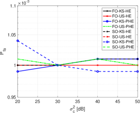
(a) $P_{fa}$ versus $\sigma_{c}^{2}$.

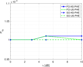
(b) $P_{fa}$ versus $\gamma$.

Figure 1: Estimated $P_{fa}$ versus $\sigma_{c}^{2}$ (a) and $\gamma$ (b) for $N=16$, $K_{P}=16$, $K_{S}=32$, and $r=2$. The maximum number of iterations for the alternating procedure is 5. The nominal values of $\sigma_{c}^{2}$, $\gamma$, and $P_{fa}$ are $30$ dB, $3$ dB, and $10^{-3}$, respectively.

The analysis starts by assessing to what extent the detection thresholds are sensitive to the variations of $\sigma_{c}^{2}$ and $\gamma$. The results are shown in Figure 1, where we plot the estimated $P_{fa}$ over $100/P_{fa}$ MC trials assuming a nominal value of $10^{-3}$. These results indicate that $P_{fa}$ for all the derived detectors is relatively invariant to $\sigma_{c}^{2}$ and $\gamma$, at least for the considered parameter settings.

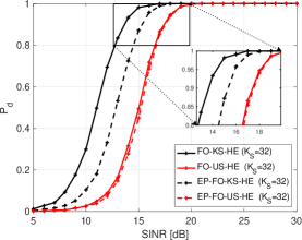
Figure 2: First-order detectors for homogeneous environment: $N=16,K_{P}=16,r=2$, and $K_{S}=32$.

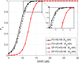
Figure 3: First-order detectors for homogeneous environment: $N=16,K_{P}=16,r=2$, and $K_{S}=64$.

Figures 2-5 are plots of $P_{d}$ vs SINR for the first-order GLR detectors and their EP approximations. Figures 2 and 3 assume a homogeneous environment and 4 and 5 assume a partially-homogeneous environment. The GLR detectors of [1] are represented by solid lines and the EP approximations are represented by dashed lines. Curves of detectors for a known signal subspace are black and curves of detectors for an unknown subspace are red. A zoom box on high values of $P_{d}$ demonstrates the gains/losses at $P_{d}=0.9$. Inspection of the figures shows that detectors for a known signal subspace outperform detectors for an unknown subspace, as could be expected. More importantly, GLR detectors for a known signal subspace outperform their EP approximations. The GLR and EP detectors are more or less equivalent under the assumption that the signal subspace is unknown.

To show the influence of $K_{S}$ on the detection performance, one can compare Figures 2 and 3 for the homogeneous environment and, similarly, Figures 4 and 5 for the partially-homogeneous environment. The comparisons highlight the better performance obtained for the greater value of $K_{S}$ for all detectors, with the EP detectors filling the performance gap at $K_{S}=64$ due to an enhanced fidelity of the SCM estimate. Additional numerical examples not reported here for brevity confirm the observed behavior for $r=4$.

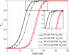
Figure 4: First-order detectors for partially-homogeneous environment: $N=16,K_{P}=16,r=2$, and $K_{S}=32$.

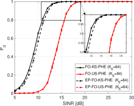
Figure 5: First-order detectors for partially-homogeneous environment: $N=16,K_{P}=16,r=2$, and $K_{S}=64$.

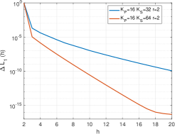
(a) Homogeneous Environment ($H_{0}$).

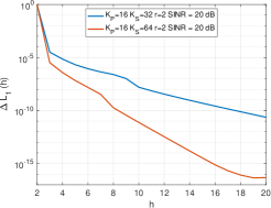
(b) Homogeneous Environment ($H_{1}$).

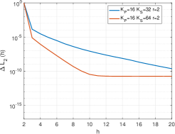
(c) Partially-Homogeneous Environment ($H_{0}$).

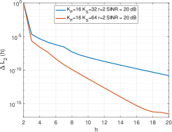
(d) Partially-Homogeneous Environment ($H_{1}$).

Figure 6: Log-likelihood variation versus the iteration number of the alternating procedures.

III-B Second order models

Under the second-order model, $\bm{\alpha}=[\alpha_{1},\dots,\alpha_{K_{P}}]^{T}$ is a complex Gaussian vector with covariance matrix $\sigma_{\alpha}^{2}{\mbox{\boldmath$I$}}_{K_{P}}$, with $\sigma^{2}_{\alpha}>0$ varying according to the SINR defined in (25) with $\sigma_{\alpha}^{2}$ replacing $|\alpha|^{2}$.

As a preliminary step, we analyze the proposed alternating procedures for iterations $h$, ranging from 2 to 20. To this end, we plot the average values of $\Delta L_{i}$, $i=1,2$, over 100 MC trials versus $h$, in Figures 6(a)-6(d), for both the homogeneous and the partially-homogeneous environments and simulating the null and the alternative hypotheses. All the parameter values used for this analysis are shown in the figures; under $H_{1}$ the SINR value is set to $20$ dB. It turns out that, for the considered parameters, 5 iterations are sufficient to achieve a relative variation approximately lower than $10^{-5}$ and this value is also used in what follows.

Figures 7-10 are plots of $P_{d}$ vs SINR for the second-order GLR detectors and their EP approximations. Figures 7 and 8 assume a homogeneous environment and 9 and 10 assume a partially-homogeneous environment. The GLR detectors proposed in [1] are represented by solid lines and the EP approximations are represented by dashed lines. Curves of detectors for a known signal subspace are blue and curves of detectors for an unknown subspace are green. Again a zoom box on high values of $P_{d}$ is reported. The second-order detectors for a known signal subspace outperform detectors for an unknown signal subspace and GLR detectors for a known signal subspace are better than the corresponding EP detectors for $K_{S}=32$. However, this time the gain of the GLR detector over the corresponding EP detector is much more pronounced in a partially-homogeneous environment and, in the case of detectors for a known subspace, is still remarkable for $K_{S}=64$.

IV Conclusions

In this paper, we have assessed the performance of the GLR detectors derived in the companion paper [1] and compared the performance of these detectors to the performance of EP approximations. It is worth noticing that most of the EP approximations have been derived here for the first time (at least to the best of authors’ knowledge). As in [1], we have considered two operating situations: a homogeneous environment where training samples and testing samples share the same statistical characterization of the interference, and a partially-homogeneous environment where training and testing samples differ in scale. The analysis starts by investigating to what extent the $P_{fa}$ is sensitive to variations of the clutter parameters showing that all the GLR detectors maintain a rather constant false alarm rate over the considered parameter ranges. When the signal subspace is known, performance is better than when it is known only by its dimension. The GLR detectors outperform their EP approximants in case the signal subspace is known and the number of secondary data is not too large. Finally, the performance of the detectors for an unknown signal subspace are close to each other. Summarizing, the analysis has shown that the design framework proposed in [1] leads to effective solutions for signals with inherent uncertainty that, for a specific radar application, can be related to the angles of arrival, Doppler frequency, and/or phase/amplitude calibration errors. Future research might analyze these detectors on real data and under a mismatch between the actual and the nominal signal subspace.

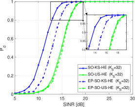
Figure 7: Second-order detectors for homogeneous environment: $N=16,K_{P}=16,r=2$, and $K_{S}=32$.

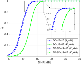
Figure 8: Second-order detectors for homogeneous environment: $N=16,K_{P}=16,r=2$, and $K_{S}=64$.

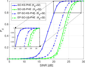
Figure 9: Second-order detectors for partially-homogeneous environment: $N=16,K_{P}=16,r=2$, and $K_{S}=32$.

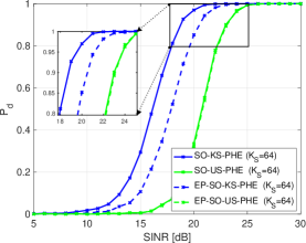
Figure 10: Second-order detectors for partially-homogeneous environment: $N=16,K_{P}=16,r=2$, and $K_{S}=64$.

References

• [1] D. Orlando, G. Ricci, and L. L. Scharf, “A Unified Theory of Adaptive Subspace Detection - Part I: Detector Designs,” IEEE Transactions on Signal Processing, 2021, under review.
• [2] F. Bandiera, A. De Maio, A. S. Greco, and G. Ricci, “Adaptive Radar Detection of Distributed Targets in Homogeneous and Partially Homogeneous Noise Plus Subspace Interference,” IEEE Transactions on Signal Processing, vol. 55, no. 4, pp. 1223–1237, 2007.
• [3] F. Bandiera, O. Besson, D. Orlando, G. Ricci, and L. L. Scharf, “GLRT-based direction detectors in homogeneous noise and subspace interference,” IEEE Transactions on Signal Processing, vol. 55, no. 6, pp. 2386–2394, 2007.
• [4] L. L. Scharf and B. Friedlander, “Matched subspace detectors,” IEEE Transactions on Signal Processing, vol. 42, no. 8, pp. 2146–2157, 1994.
• [5] L. Scharf, S. Kraut, and M. McCloud, “A review of matched and adaptive subspace detectors,” in Proceedings of the IEEE 2000 Adaptive Systems for Signal Processing, Communications, and Control Symposium (Cat. No.00EX373), 2000, pp. 82–86.
• [6] Y. Hou, W. Zhu, E. Wang, and Y. Zhang, “A Hyperspectral Subspace Target Detection Method Based on AMUSE,” International Journal of Pattern Recognition and Artificial Intelligence, vol. 33, no. 12, 2019.
• [7] N. Acito, M. Moscadelli, M. Diani, and G. Corsini, “Subspace-based target detection in LWIR hyperspectral imaging,” IEEE Geoscience and Remote Sensing Letters, vol. 17, no. 6, pp. 1047–1051, 2020.
• [8] C.-I. Chang, H. Cao, and M. Song, “Orthogonal subspace projection target detector for hyperspectral anomaly detection,” IEEE Journal of Selected Topics in Applied Earth Observations and Remote Sensing, vol. 14, pp. 4915–4932, 2021.
• [9] O. Besson, A. Coluccia, E. Chaumette, G. Ricci, and F. Vincent, “Generalized likelihood ratio test for detection of gaussian rank-one signals in gaussian noise with unknown statistics,” IEEE Transactions on Signal Processing, vol. 65, no. 4, pp. 1082–1092, February 15 2017.
• [10] E. J. Kelly and K. Forsythe, “Adaptive Detection and Parameter Estimation for Multidimensional Signal Models,” Lincoln Lab, MIT, Lexington, US, Technical Report 848, 1989.
• [11] S. Kraut and L. L. Scharf, “The CFAR adaptive subspace detector is a scale-invariant GLRT,” IEEE Transactions on Signal Processing, vol. 47, no. 9, pp. 2538–2541, 1999.
• [12] M. Desai and R. Mangoubi, “Robust Gaussian and non-Gaussian matched subspace detection,” IEEE Transactions on Signal Processing, vol. 51, no. 12, pp. 3115–3127, 2003.
• [13] F. Gini and A. Farina, “Vector subspace detection in compound-gaussian clutter. Part I: survey and new results,” IEEE Transactions on Aerospace and Electronic Systems, vol. 38, no. 4, pp. 1295–1311, 2002.
• [14] G. Ricci and L. Scharf, “Adaptive radar detection of extended Gaussian targets,” in The Twelfth Annual Workshop on Adaptive Sensor Array Processing ASAP 2004.   Lincoln Laboratory, Massachusetts Institute of Technology, Lexington, Massachusetts (USA), 16-18 March 2004.
• [15] F. Robey, D. Fuhrmann, E. Kelly, and R. Nitzberg, “A CFAR adaptive matched filter detector,” IEEE Transactions on Aerospace and Electronic Systems, vol. 28, no. 1, pp. 208–216, 1992.
• [16] P. Stoica and Y. Selen, “Cyclic minimizers, majorization techniques, and the expectation-maximization algorithm: a refresher,” IEEE Signal Processing Magazine, vol. 21, no. 1, pp. 112–114, 2004.
• [17] S. Han, L. Yan, Y. Zhang, P. Addabbo, C. Hao, and D. Orlando, “Adaptive Radar Detection and Classification Algorithms for Multiple Coherent Signals,” IEEE Transactions on Signal Processing, vol. 69, pp. 560–572, 2021.
• [18] J. Ward, “Space-time adaptive processing for airborne radar,” MIT Lincoln Laboratory, Tech. Rep. 1015, 1994.
• [19] Y. Bresler, “Maximum likelihood estimation of a linearly structured covariance with application to antenna array processing,” in Fourth Annual ASSP Workshop on Spectrum Estimation and Modeling, Minneapolis, MN (USA), August 3-5 1988, pp. 172–175.
• [20] F. Bandiera, D. Orlando, and G. Ricci, Advanced Radar Detection Schemes Under Mismatched Signal Models.   Synthesis Lectures on Signal Processing, Morgan & Claypool Publishers, 2009.
• [21] P. Addabbo, S. Han, D. Orlando, and G. Ricci, “Learning Strategies for Radar Clutter Classification,” IEEE Transactions on Signal Processing, vol. 69, pp. 1070–1082, 2021.
• [22] L. Yan, P. Addabbo, C. Hao, D. Orlando, and A. Farina, “New ECCM Techniques Against Noiselike and/or Coherent Interferers,” IEEE Transactions on Aerospace and Electronic Systems, vol. 56, no. 2, pp. 1172–1188, 2020.
• [23] A. Pezeshki, B. D. Van Veen, L. L. Scharf, H. Cox, and M. Lundberg Nordenvaad, “Eigenvalue beamforming using a multirank mvdr beamformer and subspace selection,” IEEE Transactions on Signal Processing, vol. 56, no. 5, pp. 1954–1967, 2008.