Subspace Learning Machine (SLM):
Methodology and Performance

Abstract

Inspired by the feedforward multilayer perceptron (FF-MLP), decision tree (DT) and extreme learning machine (ELM), a new classification model, called the subspace learning machine (SLM), is proposed in this work. SLM first identifies a discriminant subspace, $S^{0}$, by examining the discriminant power of each input feature. Then, it uses probabilistic projections of features in $S^{0}$ to yield 1D subspaces and finds the optimal partition for each of them. This is equivalent to partitioning $S^{0}$ with hyperplanes. A criterion is developed to choose the best $q$ partitions that yield $2q$ partitioned subspaces among them. We assign $S^{0}$ to the root node of a decision tree and the intersections of $2q$ subspaces to its child nodes of depth one. The partitioning process is recursively applied at each child node to build an SLM tree. When the samples at a child node are sufficiently pure, the partitioning process stops and each leaf node makes a prediction. The idea can be generalized to regression, leading to the subspace learning regressor (SLR). Furthermore, ensembles of SLM/SLR trees can yield a stronger predictor. Extensive experiments are conducted for performance benchmarking among SLM/SLR trees, ensembles and classical classifiers/regressors.

Machine Learning, Classification, Subspace Learning

I Introduction

Feature-based classification models have been well studied for many decades. Feature extraction and classification are treated as two separate modules in the classical setting. Attention has been shifted to deep learning (DL) in recent years. Feature learning and classification are handled jointly in DL models. Although the best performance of classification tasks is broadly achieved by DL through back propagation (BP), DL models suffer from lack of interpretability, high computational cost and high model complexity. Under the classical learning paradigm, we propose new high-performance classification and regression models with features as the input in this work.

Examples of classical classifiers/regressors include support vector machine (SVM) [1], decision tree (DT) [2], multilayer perceptron (MLP) [3], feedforward multilayer perceptron (FF-MLP) [4] and extreme learning machine (ELM) [5]. SVM, DT and FF-MLP share one common idea, i.e., feature space partitioning. Yet, they achieve this objective by different means. SVM partitions the space by leveraging kernel functions and support vectors. DT partitions one space into two subspaces by selecting the most discriminant feature one at a time recursively. DT tends to overfit the training data when the tree depth is high. To avoid it, one can build multiple DTs, each of which is a weak classifier, and their ensemble yields a strong one, e.g., the random forest (RF) classifier [6]. Built upon linear discriminant analysis, FF-MLP uses the Gaussian mixture model (GMM) to capture feature distributions of multiple classes and adopts neuron pairs with weights of opposite signed vectors to represent partitioning hyperplanes.

The complexity of SVM and FF-MLP depends on the sample distribution in the feature space. It is a nontrivial task to determine suitable partitions when the feature dimension is high and/or the sample distribution is complicated. These challenges could limit the effectiveness and efficiency of SVM and FF-MLP. Selecting a partition in DTs is easier since it is conducted on a single feature. Yet, the simplicity is paid by a price. That is, the discriminant power of an individual feature is weak, and a DT results in a weak classifier. As proposed in ELM [5], another idea of subspace partitioning is to randomly project a high-dimensional space to a 1D space and find the optimal split point in the associated 1D space. Although ELM works theoretically, it is not efficient in practice if the feature dimension is high. It takes a large number of trials and errors in finding good projections. A better strategy is needed.

By analyzing pros and cons of SVM, FF-MLP, DT and ELM, we attempt to find a balance between simplicity and effectiveness and propose a new classification-oriented machine learning model in this work. Since it partitions an input feature space into multiple discriminant subspaces in a hierarchical manner, it is named the subspace learning machine (SLM). Its basic idea is sketched below. Let $X$ be the input feature space. First, SLM identifies subspace $S^{0}$ from $X$. If the dimension of $X$ is low, we set $S^{0}=X$. If the dimension of $X$ is high, we remove less discriminant features from $X$ so that the dimension of $S^{0}$ is lower than that of $X$.

Next, SLM uses probabilistic projections of features in $S^{0}$ to yield $p$ 1D subspaces and find the optimal partition for each of them. This is equivalent to partitioning $S^{0}$ with $2p$ hyperplanes. A criterion is developed to choose the best $q$ partitions that yield $2q$ partitioned subspaces among them. We assign $S^{0}$ to the root node of a decision tree and the intersections of $2q$ subspaces to its child nodes of depth one. The partitioning process is recursively applied at each child node to build an SLM tree until stopping criteria are met, then each leaf node makes a prediction. Generally, an SLM tree is wider and shallower than a DT. The prediction capability of an SLM tree is stronger than that of a single DT since it allows multiple decisions at a decision node. Its performance can be further improved by ensembles of multiple SLM trees obtained by bagging and boosting. The idea can be generalized to regression, leading to the subspace learning regressor (SLR). Extensive experiments are conducted for performance benchmarking among individual SLM/SLR trees, multi-tree ensembles and several classical classifiers and regressors. They show that SLM and SLR offer light-weight high-performance classifiers and regressors, respectively.

The rest of this paper is organized as follows. The SLM model is introduced in Sec. II. The ensemble design is proposed in Sec. III. Performance evaluation and benchmarking of SLM and popular classifiers are given in Sec. IV. The generalization to SLR is discussed in Sec. V. The relationship between SLM/SLR and other machine learning methods such as classification and regression tree (CART), MLP, ELM, RF and Gradient Boosting Decision Tree (GBDT) [7] is described in Sec. VI. Finally, concluding remarks are given in Sec. VII.

II Subspace Learning Machine (SLM)

II-A Motivation

Consider an input feature space, $X$, containing $L$ samples, where each sample has a $D$-dimensional feature vectors. A sample is denoted by

$$\bm{x}_{l}=(x_{l,1}\cdots x_{l,d}\cdots,x_{l,D})^{T}\in\mathbb{R}^{D},$$ (1)

where $l=1,\cdots,L$. We use $F_{d}$ to represent the $d$th feature set of $\bm{x}_{l}$, i.e.,

$$F_{d}=\{x_{l,d}\mid 1\leq l\leq L\}.$$ (2)

For a multi-class classification problem with $K$ classes, each training feature vector has an associated class label in form of one-hot vector

$$\bm{y}_{l}=(y_{l,1},\cdots,y_{l,k},\cdots,y_{l,K})^{T}\in\mathbb{R}^{K},$$ (3)

where

$$y_{l,k}=1\mbox{ and }y_{l,k^{\prime}}=0,k^{\prime}\neq k,$$ (4)

if the $l$th sample belongs to class $k$, where $1\leq k,k^{\prime}\leq K$. Our goal is to partition the feature space, $\mathbb{R}^{D}$, into multiple subspaces hierarchically so that samples at leaf nodes are as pure as possible. It means that the majority of samples at a node is from the same class. Then, we can assign all samples in the leaf node to the majority class. This process is adopted by a DT classifier. The root node is the whole sample space, and an intermediate or leaf node corresponds to a partitioned subspace. We use $S^{0}$ to represent the sample space at the root node and $S^{m}$, $m=1,\cdots,M$, to denote subspaces of child nodes of depth $m$ in the tree.

The efficiency of traditional DT methods could be potentially improved by two ideas. They are elaborated below.

1. Partitioning in flexibly chosen 1D subspace:
   We may consider a general projected 1D subspace defined by

   $$F_{\bm{a}}=\{f(\bm{a})\mid f(\bm{a})=\bm{a}^{T}\bm{x}\},$$ (5)

   where

   $$\bm{a}=(a_{1},\cdots,a_{d},\cdots,a_{D})^{T},\hskip 14.22636pt||\bm{a}||=1,$$ (6)

   The DT is a special case of Eq. (5), where $\bm{a}$ is set to the $d$th basis vector, $\bm{e}_{d}$, $1\leq d\leq D$. On one hand, this choice simplifies computational complexity, which is particularly attractive if $D>>1$. On the other hand, if there is no discriminant feature $F_{d}$, the decision tree will not be effective. It is desired to find a discriminant direction, $\bm{a}$, so that the subspace, $F_{\bm{a}}$, has a more discriminant power at a low computational cost.

2. N-ary split at one node:
   One parent node in DT is split into two child nodes. We may allow an n-ary split at the parent. One example is shown in Fig. 1(a) and (b), where space $S^{0}$ is split into four disjoint subspaces. Generally, the n-ary split gives wider and shallower decision trees so that overfitting can be avoided more easily.

The SLM method is motivated by these two ideas. Although the high-level ideas are straightforward, their effective implementations are nontrivial. They will be detailed in the next subsection.

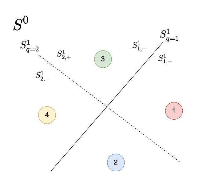
(a)

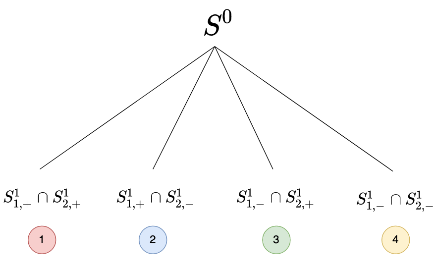
(b)

Figure 1: (a) An illustration of SLM, where space $S^{0}$ is partitioned into 4 subspaces with two splits, and (b) the corresponding SLM tree with a root note and four child nodes.

II-B Methodology

Subspace partitioning in a high-dimensional space plays a fundamental role in the design of powerful machine learning classifiers. Generally, we can categorize the partitioning strategies into two types: 1) search for an optimal split point in a projected 1D space (e.g., DT) and 2) search for an optimal splitting hyperplane in a high-dimensional space (e.g., SVM and FF-MLP). Mathematically, both of them can be expressed in form of

$$\bm{a}^{T}\bm{x}-b=0,$$ (7)

where $-b$ is called the bias and

$$\bm{a}=(a_{1},\cdots,a_{d},\cdots,a_{D})^{T},\hskip 14.22636pt||\bm{a}||=1,$$ (8)

is a unit normal vector that points to the surface normal direction. It is called the projection vector. Then, the full space, $S$, is split into two half subspaces:

$$S_{+}:\,\bm{a}^{T}\bm{x}\geq b,\mbox{ and }S_{-}:\,\bm{a}^{T}\bm{x}<b.$$ (9)

The challenge lies in finding good projection vector $\bm{a}$ so that samples of different classes are better separated. It is related to the distribution of samples of different classes. For the first type of classifiers, they pre-select a set of candidate projection vectors, try them out one by one, and select the best one based on a certain criterion. For the second type of classifiers, they use some criteria to choose good projection vectors. For example, SVM first identifies support vectors and then finds the hyperplane that yields the largest separation (or margin) between two classes. The complexity of the first type is significantly lower than that of the second type.

In SLM, we attempt to find a mid-ground of the two. That is, we generate a new 1D space as given by

$$F_{\bm{a}}=\{f(\bm{a})\mid f(\bm{a})=\bm{a}^{T}\bm{x}\},$$ (10)

where $\bm{a}$ is a vector on the unit hypersphere in $\mathbb{R}^{D}$ as defined in Eq. (8). By following the first type of classifier, we would like to identify a set of candidate projection vectors. Yet, their selection is done in a probabilistic manner. Generally, it is not effective to draw $\bm{a}$ on the unit hypersphere uniformly. The criterion of effective projection vectors and their probalisitic selection will be presented in Secs. II-B1-II-B3. Without loss of generality, we primarily focus on the projection vector selection at the root node in the following discussion. The same idea can be easily generalized to child nodes.

II-B1 Selection Criterion

We use the discriminant feature test (DFT) [8] to evaluate the discriminant quality of the projected 1D subspace as given in Eq. (10). It is summarized below.

For a given projection vector, $\bm{a}$, we find the minimum and the maximum of projected values $f(\bm{a})=\bm{a}^{T}\bm{x}$, which are denoted by $f_{\min}$ and $f_{\max}$, respectively. We partition interval $[f_{\min},f_{\max}]$ into $B$ bins uniformly and use bin boundaries as candidate thresholds. One threshold, $t_{b}$, $b=1,\cdots,B-1$, partitions interval $[f_{\min},f_{\max}]$ into two subintervals that define two sets:

$$F_{\bm{a},t_{b},+} = \{f(\bm{a})\mid\bm{a}^{T}\bm{x}\geq t_{b}\},$$ (11)

$$F_{\bm{a},t_{b},-} = \{f(\bm{a})\mid\bm{a}^{T}\bm{x}<t_{b}\}.$$ (12)

The bin number, $B$, is typically set to 16 [8].

The quality of a split can be evaluated with the weighted sum of loss functions defined on the left and right subintervals:

$$\mathcal{L}_{\bm{a},t_{b}}=\frac{N_{+}}{N_{+}+N_{-}}\mathcal{L}_{\bm{a},t_{b},+}+\frac{N_{-}}{N_{+}+N_{-}}\mathcal{L}_{\bm{a},t_{b},-},$$ (13)

where $N_{+}=\mid F_{\bm{a},t_{b},+}\mid$ and $N_{-}=\mid F_{\bm{a},t_{b},-}\mid$ are sample numbers in the left and right subintervals, respectively. One convenient choice of the cost function is the entropy value as defined by

$$\mathcal{L}=-\sum^{C}_{c=1}p_{c}\log(p_{c}),$$ (14)

where $p_{c}$ is the probability of samples in a certain set belonging to class $c$ and $C$ is the total number of classes. In practice, the probability is estimated using the histogram. Finally, the discriminant power of a certain projection vector is defined as the minimum cost function across all threshold values:

$$\mathcal{L}_{\bm{a},\mbox{opt}}=\min_{t_{b}}\mathcal{L}_{\bm{a},t_{b}}.$$ (15)

We search for projection vectors, $\bm{a}$ that provide small cost values as give by Eq. (15). The smaller, the better.

II-B2 Probabilistic Selection

We adopt a probabilistic mechanism to select one or multiple good projection vectors. To begin with, we express the project vector as

$$\bm{a}=a_{1}\bm{e}_{1}+\cdots,a_{d}\bm{e}_{d}+\cdots+a_{D}\bm{e}_{D},$$ (16)

where $\bm{e}_{d}$, $d=1,\cdots,D$, is the basis vector. We evaluate the discriminant power of $\bm{e}_{d}$ by setting $\bm{a}=\bm{e}_{d}$ and following the procedure in Sec. II-B1. Our probabilistic selection scheme is built upon one observation. The discriminability of $\bm{e}_{d}$ plays an important role in choosing a more discriminant $\bm{a}$. Thus, we rank $\bm{e}_{d}$ according to their discriminant power measured by the cost function in Eq. (15). The newly ordered basis is denoted by $\bm{e^{\prime}}_{d}$, $d=1,\cdots,D$, which satisfies the following:

$$\mathcal{L}_{\bm{e^{\prime}}_{1},\mbox{opt}}\leq\mathcal{L}_{\bm{e^{\prime}}_{2},\mbox{opt}}\leq\cdots\leq\mathcal{L}_{\bm{e^{\prime}}_{D},\mbox{opt}}.$$ (17)

We can rewrite Eq. (16) as

$$\bm{a}=a^{\prime}_{1}\bm{e^{\prime}}_{1}+\cdots,a^{\prime}_{d}\bm{e^{\prime}}_{d}+\cdots+a^{\prime}_{D}\bm{e^{\prime}}_{D}.$$ (18)

We use three hyper-parameters to control the probabilistic selection procedure.

• $P_{d}$: the probability of selecting coefficient $a^{\prime}_{d}$
  Usually, $P_{d}$ is higher for smaller $d$. In the implementation, we adopt the exponential density function in form of

  $$P_{d}=\beta_{0}\exp(-\beta d),$$ (19)

  where $\beta>0$ is a parameter and $\beta_{0}$ is the corresponding normalization factor.

• $A_{d}$: the dynamic range of coefficient $a^{\prime}_{d}$
  To save the computation, we limit the values of $a^{\prime}_{d}$ and consider integer values within the dynamic range; namely,

  $$a^{\prime}_{d}=0,\pm 1,\,\pm 2,\,\cdots,\,\pm\lfloor A_{d}\rfloor,$$ (20)

  where $A_{d}$ is also known as the envelop parameter. Again, we adopt the exponential density function

  $$A_{d}=\alpha_{0}\exp(-\alpha d),$$ (21)

  where $\alpha>0$ is a parameter and $\alpha_{0}$ is the corresponding normalization factor in the implementation. When the search space in Eq. (20) is relatively small with chosen hyperparameters, we exhaustively test all the values. Otherwise, we select a partial set of the orientation vector coefficients probabilistically under the uniform distribution.

• $R$: the number of selected coefficients, $a^{\prime}_{d}$, in Eq (18)
  If $D$ is large, we only select a subset of $R$ coefficients, where $R<<D$ to save computation. The dynamic ranges of the remaining $(D-R)$ coefficients are all set to zero.

By fixing parameters $\beta$, $\alpha$ and $R$ in one round of $\bm{a}$ generation, the total search space of $\bm{a}$ to be tested by DFT lies between

$$\mbox{U.B.}=\Pi_{d=1}^{R}(2A_{d}+1),\quad\mbox{L.B.}=\Pi_{d=D+1-R}^{D}(2A_{d}+1),$$ (22)

where U.B and L.B. mean upper and lower bounds, respectively. To increase the diversity of $\bm{a}$ furthermore, we may use multiple rounds in the generation process with different $\beta$, $\alpha$ and $R$ parameters.

We use Fig. 2 as an example to illustrate the probabilistic selection process. Suppose input feature dimension $D=10$ and $R$ is selected as 5, we may apply $\alpha_{0}$ as 10 and $\alpha$ as 0.5 for bounding the dynamic range of the $a^{\prime}_{d}$ selections. During the probabilistic selection, the $R=5$ coefficients are selected with the candidate integers for the corresponding $a^{\prime}_{d}$ marked as black dots, the unselected $D-R$ coefficients are marked as gray and the actual coefficients are set to zero. The coefficients of the orientation vector $\bm{a}$ are uniformly selected among the candidate integers marked as black dots in Fig. 2.

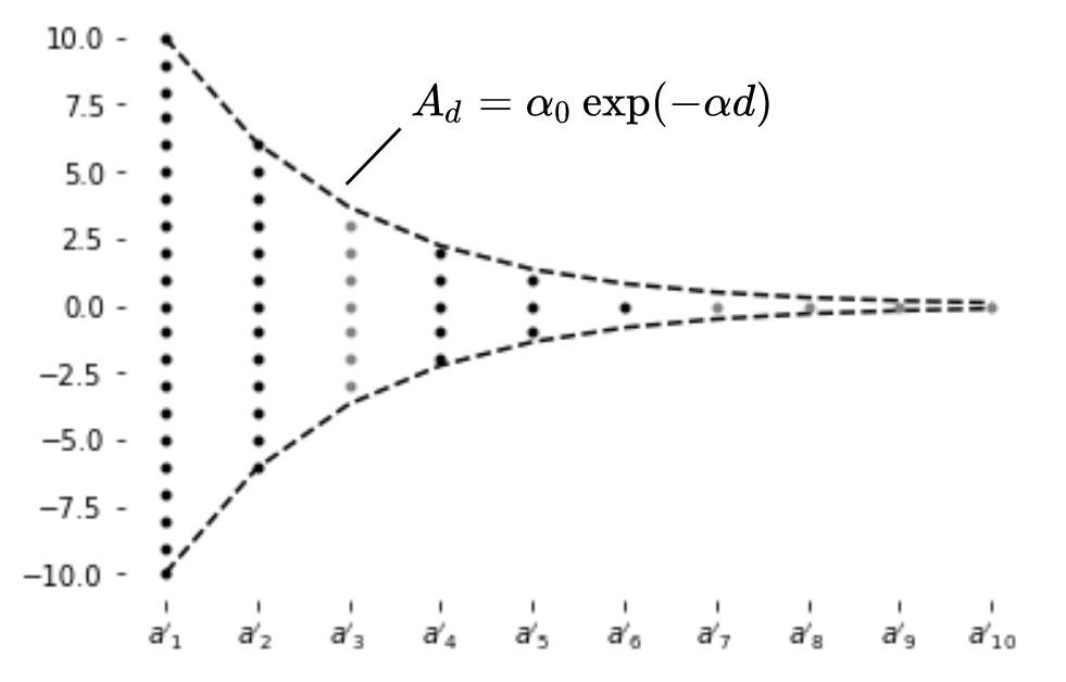
Figure 2: Illustration of the probabilistic selection process, where the envelop function $A_{d}$ that provides a bound on the magnitude of coefficients $a^{\prime}_{d}$ in the orientation vector. The dimensions with black dots are selected dimensions, and dots in one vertical line are integers for selection for each dimension. In this example, the selected dimensions are $a^{\prime}_{1}$, $a^{\prime}_{2}$, $a^{\prime}_{4}$, $a^{\prime}_{5}$ and $a^{\prime}_{6}$. For each trial, we select one black dot per vertical line to form an orientation vector. The search can be done exhaustively or randomly with the uniform distribution.

II-B3 Selection of Multiple Projection Vectors

Based on the search given in Sec. II-B2, we often find multiple effective projection vectors

$$\bm{\tilde{a}}_{j},j=1,\cdots,J,$$ (23)

which yield discriminant 1D subspaces. It is desired to leverage them as much as possible. However, many of them are highly correlated in the sense that their cosine similarity measure is close to unity, i.e.,

$$\bm{\tilde{a}}_{j}^{T}\bm{\tilde{a}}_{j^{\prime}}\approx 1.$$ (24)

As a result, the correspondidg two hyperplanes have a small angle between them. To avoid this, we propose an iterative procedure to select multiple projection vectors. To begin with, we choose the projection vector in Eq. (23) that has the smallest cost as the first one. Next, we choose the second one from Eq. (23) that minimizes its absolute cosine similarity value with the first one. We can repeat the same process by minimizing the maximum cosine similarities with the first two, etc. The iterative mini-max optimization process can be terminated by a pre-defined threshold value, $\theta_{minimax}$.

II-B4 SLM Tree Construction

We illustrate the SLM tree construction process in Fig. 3. It contains the following steps.

1. Check the discriminant power of ${D}$ input dimensions and find discriminant input subspace ${S}^{0}$ with ${D}_{0}$ dimensions among D.

2. Generate $p$ projection vectors that project the selected input subspace to $p$ 1D subspaces. The projected space is denoted by $\tilde{S}$.

3. Select the best $q$ 1D spaces from $p$ candidate subspaces based on discriminability and correlation and split the node accordingly, which is denoted by $S^{1}$.

The node split process is recursively conducted to build nodes of the SLM tree. The following stopping criteria are adopted to avoid overfitting at a node.

1. The depth of the node is greater than user’s pre-selected threshold (i.e. the hyper-parameter for the maximum depth of an SLM tree).

2. The number of samples at the node is less than user’s pre-selected threshold (i.e. the hyper-parameter for the minimum sample number per node).

3. The loss at the node is less than user’s pre-selection threshold (i.e. the hyper-parameter for the minimum loss function per node).

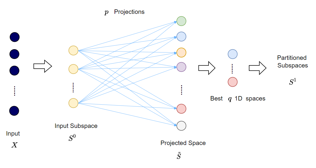
Figure 3: An overview of the SLM system.

III SLM Forest and SLM Boost

Ensemble methods are commonly used in the machine learning field to boost the performance. An ensemble model aims to obtain better performance than each constituent model alone. With DTs as the constituent weak learners, the bootstrap aggregating or bagging method, (e.g., RF) and the boosting method (e.g. GBDT) are the most popular ensemble methods. As compared to other classical machine learning methods, they often achieve better performance when applied to real world applications. In this section, we show how to apply the ensemble idea to one single SLM tree (i.e., SLM Baseline). Inspired by RF, we present a bagging method for SLM and call it the SLM Forest. Similarly, inspired by XGBoost [9, 10], we propose a boosting method and name it SLM Boost. They are detailed in Secs. III-A and III-B, respectively.

III-A SLM Forest

For traditional DTs, RF is the most popular bagging ensemble algorithm. It consists of a set of tree predictors, where each tree is built based on the values of a random vector sampled independently and with the same distribution for all trees in the forest [6]. With the Strong Law of Large Numbers, the performance of RF converges as the tree number increases. As compared to the individual DTs, significant performance improvement is achieved with the combination of many weak decision trees. Motivated by RF, SLM Forest is developed by learning a series of single SLM tree models to enhance the predictive performance of each individual SLM tree. As discussed in Sec. II, SLM is a predictive model stronger than DT. Besides, the probabilistic projection provides diversity between different SLM models. Following RF, SLM Forest takes the majority vote of the individual SLM trees as the ensemble result for classification tasks, and it adopts the mean of each SLM tree prediction as the ensemble result for regression tasks.

It is proved in [11] that the predictive performance of RF depends on two key points: 1) the strength of individual trees, and 2) the weak dependence between them. In other words, a high performance RF model can be obtained through the combination of strong and uncorrelated individual trees. The model diversity of RF is achieved through bagging of the training data and feature randomness. For the former, RF takes advantage of the sensitivity of DTs to the data they are trained on, and allows each individual tree to randomly sample from the dataset with replacement, resulting in different trees. For the latter, each tree can select features only from a random subset of the whole input features space, which forces diversity among trees and ultimately results in lower correlation across trees for better performance.

SLM Forest achieves diversity of SLM trees more effectively through probabilistic selection as discussed in Sec. II-B2. For partitioning at a node, we allow a probabilistic selection of ${D}_{0}$ dimensions from the $D$ input feature dimensions by taking the discriminant ability of each feature into account. In Eq. (19), $\beta$ is a hyper-parameter used to control the probability distribution among input features. A larger $\beta$ value has higher preference on more discriminant features. Furthermore, the envelope vector, $\bm{A}_{d}$ in Eq. (21) gives a bound to each element of the orientation vector. It also attributes to the diversity of SLM trees since the search space of projection vectors are determined by hyper-parameter $\alpha$. Being similar to the replacement idea in RF, all training samples and all feature dimensions are kept as the input at each node splitting to increase the strength of individual SLM trees.

With individual SLM trees stronger than individual DTs and novel design in decorrelating partitioning planes, SLM Forest achieves better performance and faster converge than RF. This claim is supported by experimental results in Sec. IV.

III-B SLM Boost

With standard DTs as weak learners, GBDT [7] and XGBoost [9, 10] can deal with a large amount of data efficiently and achieve the state-of-the-art performance in many machine learning problems. They take the ensemble of standard DTs with boosting, i.e. by defining an objective function and optimizing it with learning a sequence of DTs. By following the gradient boosting process, we propose SLM Boost to ensemble a sequence of SLM trees.

Mathematically, we aim at learning a sequence of SLM trees, where the $t$th tree is denoted by $f_{t}({\bf x})$. Suppose that we have $T$ trees at the end. Then, the prediction of the ensemble is the sum of all trees, i.e. each of the $L$ samples is predicted as

$$\hat{y}_{l} = \sum^{T}_{t=1}f_{t}({\bf x}_{l})\quad l=1,2,\cdots,L.$$ (25)

The objective function for the first $t$ trees is defined as

$$\Omega=\sum^{L}_{l=1}\gamma({y}_{l},\hat{y}_{l}^{(t)}),$$ (26)

where $\hat{y}_{l}^{(t)}$ is the prediction of sample $l$ with all $t$ trees and $\gamma({y}_{l},\hat{y}_{l}^{(t)})$ denotes the training loss for the model with a sequence of $t$ trees. The log loss and the mean squared error are commonly utilized for classification and regression tasks as the training loss, respectively. It is intractable to learn all trees at once. To design SLM Boost, we follow the GBDT process and use the additive strategy. That is, by fixing what have been learned with all previous trees, SLM Boost learns a new tree at each time. Without loss of generality, we initialize the model prediction as 0. Then, the learning process is

$$\hat{y}_{l}^{(0)} = 0$$ (27)

$$\hat{y}_{l}^{(1)} = f_{1}({\bf x}_{l})=\hat{y}_{l}^{(0)}+f_{1}(\bf{x}_{l})$$ (28)

$$\cdots$$ (29)

$$\hat{y}_{l}^{(t)} = \sum^{t}_{i=1}f_{i}({\bf x}_{l})=\hat{y}_{l}^{(t-1)}+f_{t}(x_{l})$$ (30)

Then, the objective function to learn the $t$th tree can be written as

$$\Psi(t)=\sum^{L}_{l=1}\gamma({y}_{l},\hat{y}_{l}^{(t-1)}+f_{t}({\bf x}_{l})).$$ (31)

Furthermore, we follow the XGBoost process and take the Taylor Expansion of the loss function up to the second order to approximate the loss function in general cases. Then, the objective function can be approximated as

$$\Psi^{(t)}\approx\sum^{L}_{l=1}(\gamma({y}_{l},\hat{y}_{l}^{(t-1)})+g_{l}f_{t}({\bf x}_{l})+\frac{1}{2}h_{l}f^{2}_{t}({\bf x}_{l}))+C,$$ (32)

where $g_{l}$ and $h_{l}$ are defined as

$$g_{l} = \partial_{\hat{y}_{l}^{(t-1)}}\gamma({y}_{l},\hat{y}_{l}^{(t-1)})$$ (33)

$$h_{l} = \partial^{2}_{\hat{y}_{l}^{(t-1)}}\gamma({y}_{l},\hat{y}_{l}^{(t-1)})$$ (34)

After removing all constants, the objective function for the $t$th SLM tree becomes

$$\sum^{L}_{l=1}[g_{l}f_{t}({\bf x}_{l})+\frac{1}{2}h_{l}f^{2}_{t}({\bf x}_{l})]$$ (35)

With individual SLM trees stronger than individual DTs, SLM Boost achieves better performance and faster convergence than XGBoost as illustrated by experimental results in Sec. IV.

IV Performance Evalution of SLM

TABLE I: Classification accuracy comparison of 10 benchmarking methods on nine datasets.

Datasets	circle-and-ring	2-new-moons	4-new-moons	Iris	Wine	B.C.W.	Pima	Ionosphere	Banknote
FF-MLP	87.25	91.25	95.38	98.33	94.44	94.30	73.89	89.36	98.18
BP-MLP	88.00	91.25	87.00	64.67	79.72	97.02	75.54	84.11	88.38
LSVM	48.50	85.25	85.00	96.67	98.61	96.49	76.43	86.52	99.09
SVM/RBF	88.25	89.75	88.38	98.33	98.61	97.36	75.15	93.62	100.00
DT	85.00	87.25	94.63	98.33	95.83	94.74	77.07	89.36	98.00
SLM Baseline	88.25	91.50	95.63	98.33	98.61	97.23	77.71	90.07	99.09
RF	87.00	90.50	96.00	98.33	100.00	95.61	79.00	94.33	98.91
XGBoost	87.50	91.25	96.00	98.33	100.00	98.25	75.80	91.49	99.82
SLM Forest	88.25	91.50	96.00	98.33	100.00	97.36	79.00	95.71	100.00
SLM Boost	88.25	91.50	96.00	98.33	100.00	98.83	77.71	94.33	100.00

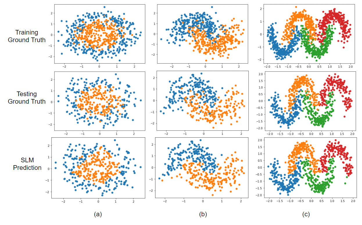
Figure 4: Visualization of 2D feature datasets: (a) Circle & Ring (b) 2-new-moon, (c) 4-new-moon. One ground truth sample of the training data, the ground truth of the test data and the SLM predicted results are shown in the first, second and third rows, respectively.

Datasets. To evaluate the performance of SLM, we conduct experiments on the following nine datasets.

1. Circle-and-Ring. It contains an inner circle as one class and an outer ring as the other class as shown in Fig. 4(a) [12].

2. 2-New-Moons. It contains two interleaving new moons as shown in Fig. 4(b) [12]. Each new moon corresponds to one class.

3. 4-New-Moons. It contains four interleaving new moons as shown in Fig. 4(c) [12], where each moon is a class.

4. Iris Dataset. The Iris plants dataset [12, 13] has 3 classes, 4D features and 150 samples.

5. Wine Dataset. The Wine recognition dataset [12, 14] has 3 classes, 13D features, and 178 samples.

6. B.C.W. Dataset. The breast cancer Wisconsin (B.C.W.) dataset [12, 14] has 2 classes, 30D features and 569 samples.

7. Diabetes Dataset. The Pima Indians diabetes dataset [15] is for diabetes prediction. It has 2 classes, 8D features and 768 samples. By following [4], we removed samples with the physically impossible zero value for glucose, diastolic blood pressure, triceps skin fold thickness, insulin, or BMI and used the remaining 392 samples for consistent experimental settings.

8. Ionosphere Dataset. The Ionosphere binary classification dataset [16, 14] is used to predict whether the radar return is good or bad. It has 2 classes, 34D features and 351 instances. For consistency with [4], we remove the feature dimension that has the zero variance from the data.

9. Banknote Dataset. The banknote authentication dataset [14] classifies whether a banknote is genuine or forged based on the features extracted from the wavelet transform of banknote images. It has 2 classes, 4D features and 1372 samples.

The feature dimension of the first three datasets is two while that of the last six datasets is higher than two. The first three are synthetic ones, where 500 samples per class are generated with 30% noisy samples in the decision boundary for 2-New-Moons and 20% noisy samples in the decision boundary of Circle-and-Ring and 4-New-Moons. The last six are real-world datasets. Samples in all datasets are randomly split into training and test sets with 60% and 40%, respectively.

Benchmarking Classifiers and Their Implementations. We compare the performance of 10 classifiers in Table I. They include seven traditional classifiers and three proposed SLM variants. The seven classifiers are: 1) MLP designed in a feedforward manner (denoted by FF-MLP) [4], 2) MLP trained by backpropagation (denoted by BP-MLP), 3) linear SVM (LSVM), 4) SVM with thee radial basis function (SVM/RBF) kernel, and 5) Decision Tree (DT) 6) Random Forest (RF) and 7) XGBoost. The three SLM variants are: 1) SLM Baseline using only one SLM tree, 2) SLM Forest, and 3) SLM Boost.

For the two MLP models, the network architectures of FF-MLP and BP-MLP and their performance results are taken from [4]. FF-MLP has a four-layer network architecture; namely, one input layer, two hidden layers and one output layer. The neuron numbers of its input and output layers are equal to the feature dimension and the class number, respectively. The neuron numbers at each hidden layer are hyper-parameters determined adaptively by a dataset. BP-MLP has the same architecture as FF-MLP against the same dataset. Its model parameters are initialized by those of FF-MLP and trained for 50 epochs. For the two SVM models, we conduct grid search for hyper-parameter $C$ in LSVM and hyper-parameters $C$ and $\gamma$ in SVM/RBF for each of the nine datasets to yield the optimal performance. For the DT model, the weighted entropy is used as the loss function in node splitting. We do not set the maximum depth limit of a tree, the minimum sample number and the minimum loss decrease required as the stopping criteria. Instead, we allow the DT for each dataset to split until the purest nodes are reached in the training. For the ensemble of DT models (i.e., RF and XGBoost), we conduct grid search for the optimal tree depth and the learning rate of XGBoost to ensure that they reach the optimal performance for each dataset. The number of trees is set to 100 to ensure convergence. The hyper-parameters of SLM Baseline (i.e., with one SLM tree) include $D_{0}$, $p$, $A_{int}$, $\alpha$, $\beta$ and the minimum number of samples used in the stopping criterion. They are searched to achieve the performance as shown in I. The number of trees in SLM Forest is set to 20 due to the faster convergence of stronger individual SLM trees. The number of trees in SLM Boost is the same as that of XGBoost for fair comparison of learning curves.

Comparison of Classification Performance. The classification accuracy results of 10 classifiers are shown in Table I. We divide the 10 classifiers into two groups. The first group includes 6 basic methods: FF-MLP, BP-MLP, LSVM, SVM/RBF, DT and SLM Baseline. The second group includes 4 ensemble methods: RF, XGBoost, SLM Forest and SLM Boost. The best results for each group are shown in bold. For the first group, SLM Baseline and SVM/RBF often outperform FF-MLP, BP-MLP, LSVM and DT and give the best results. For the three synthetic 2D datasets (i.e. circle-and-ring, 2-new-moons and 4-new-moons), the gain of SLM over MLP is relatively small due to noisy samples. The difference in sample distributions of training and test data plays a role in the performance upper bound. To demonstrate this point, we show sample distributions of their training and testing data in Fig. 4. For the datasets with high dimensional input features, the SLM methods achieve better performance over the classical methods with bigger margins. The ensemble methods in the second group have better performance than the basic methods in the first group. The ensembles of SLM are generally more powerful than those of DT. They give the best performance among all benchmarking methods.

TABLE II: Model size comparison of five machine learning models models against 9 datasets, where the smallest model size for each dataset is highlighted in bold.

Datasets	FF/BP-MLP	LSVM	SVM/RBF	DT	SLM Baseline	DT depth	SLM tree depth
Circle-and-Ring	125	2,965	1,425	350	39	14	4
2-new-moons	114	1,453	1,305	286	42	15	4
4-new-moons	702	2,853	2,869	298	93	11	5
Iris	47	235	343	34	20	6	3
Wine	147	453	963	26	99	4	2
B.C.W.	74	1,462	3,254	54	126	7	4
Pima	2,012	1,532	1,802	130	55	8	3
Ionosphere	278	1,017	2,207	50	78	10	2
Banknode	22	1,160	1,322	78	40	7	3

Comparison of Model Sizes. The model size is defined by the number of model parameters. The model sizes of FF/BP-MLP, LSVM, SVM/RBF, DT and SLM Baseline are compared in Table II. Since FF-MLP and BP-MLP share the same architecture, their model sizes are the same. It is calculated by summing up the weight and bias numbers of all neurons.

The model parameters of LSVM and SVM/RBF can be computed as

$$\mbox{SVM Parameter \#}=L+1+(D+2)N_{SV},$$ (36)

where $L$, $D$ and $N_{SV}$ denote the number of training samples, the feature dimension and the number of support vectors, respectively. The first term in Eq. (36) is the slack variable for each training sample. The second term denotes the bias. The last term comes from the fact that each support vector has $D$ feature dimensions, one Lagrange dual coefficient, and one class label.

The model sizes of DTs depend on the number of splits learned during the training process, and there are two parameters learned during each split for feature selection and split value respectively, the sizes of DTs are calculated as two times of the number of splits.

The size of an SLM baseline model depends on the number of partitioning hyper-planes which are determined by the training stage. For given hyper-parameter $\bm{D}_{0}$, each partitioning hyper-plane involves one weight matrix and a selected splitting threshold, with $\bm{q}_{i}$ decorrelated partitioning learned for partitioning each parent node. Then, the model size of the corresponding SLM can be calculated as

$$\mbox{SLM Parameter \#}=\sum^{M}_{i=1}\bm{q}_{i}(\bm{D}_{0}+1),$$ (37)

where $M$ is the number of partitioning hyperplanes.

Details on the model and computation of each method against each dataset are given in the appendix. It is worthwhile to comment on the tradeoff between the classification performance and the model size. For SVM, since its training involves learning the dual coefficients and slack variables for each training sample and memorization of support vectors, the model size is increasing linearly with the number of training samples and the number of support vectors. When achieving similar classification accuracy, the SVM model is heavier for more training samples. For MLPs, with high-dimension classification tasks, SLM methods outperforms the MLP models in all benchmarking datasets. For the datasets with saturated performance such as Iris, Banknote, and Ionosphere, SLM achievs better or comparable performance with less than half of the parameters of MLP. As compared to DTs, the SLM models tend to achieve wider and shallower trees, as shown in Table II. The depth of SLM trees are overall smaller than the DT models, while the number of splittings can be comparable for the small datasets, like Wine. The SLM trees tend to make more splits at reach pure leaf nodes at shallower depth. With outperforming the DTs in all the datasets, the SLM model sizes are generally smaller than the DTs as well with benefiting from the subspace partitioning process.

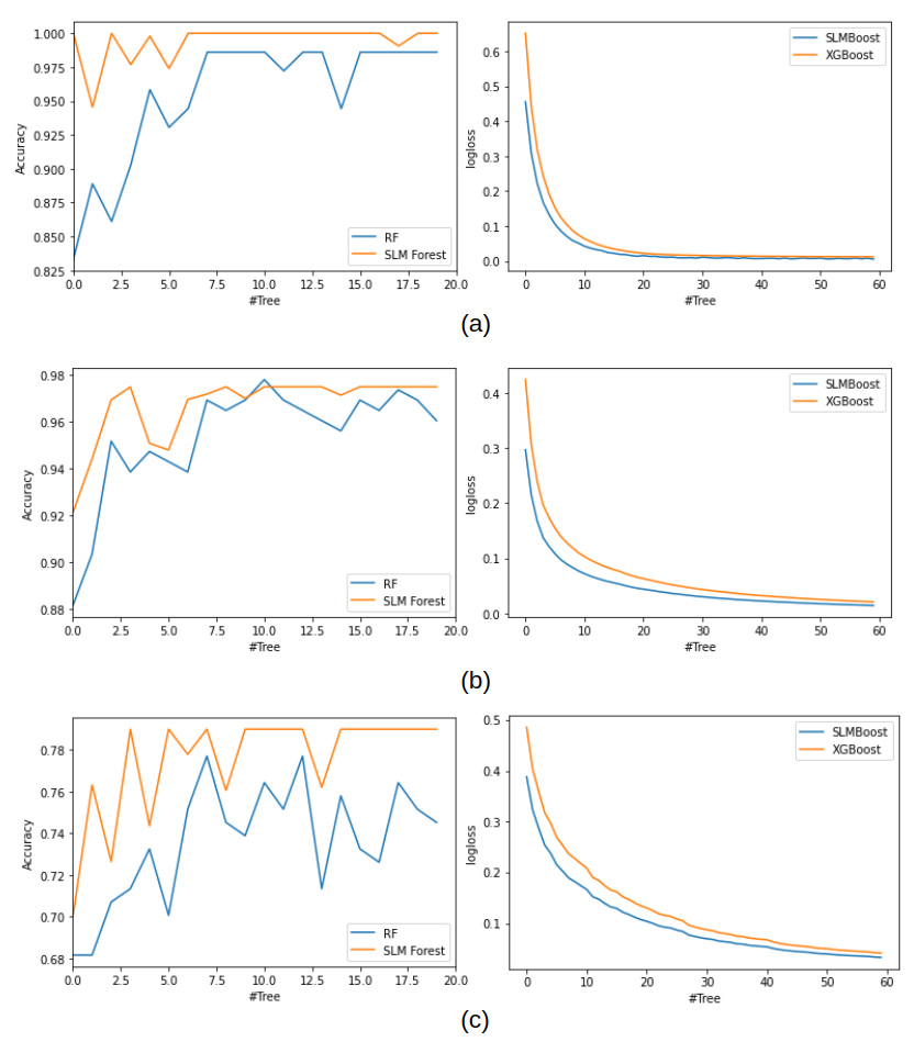
Figure 5: Comparison of SLM and DT ensembles for three datasets (a) Wine, (b) B.C.W., and (c) Pima. Each left subfigure compares the accuracy curves of SLM Forest and RF as a function of the tree number. Each right subfigure compares the logloss curves of SLM Boost and XGBoost as a function of the tree number.

TABLE III: Comparison of regression performance of eight regressors on six datasets.

Datasets	Make Friedman1	Make Friedman2	Make Friedman3	Boston	California_housing	Diabetes
LSVR	2.49	138.43	0.22	4.90	0.76	53.78
SVR/RBF	1.17	6.74	0.11	3.28	0.58	53.71
DT	3.10	33.57	0.11	4.75	0.74	76.56
SLR Baseline	2.89	31.28	0.11	4.42	0.69	56.05
RF	2.01	22.32	0.08	3.24	0.52	54.34
XGBoost	1.17	32.34	0.07	2.67	0.48	53.99
SLR Forest	1.88	20.79	0.08	3.01	0.48	52.52
SLR Boost	1.07	18.07	0.06	2.39	0.45	51.27

Convergence Performance Comparison of DT Ensembles and SLM Ensembles. We compare the convergence performance of the ensemble and the boosting methods of DT and SLM for Wine, B.C.W. and Pima three datas in Figs. 5(a)-(c). For RF and SLM Forest, which are ensembles of DT and SLM, respectively, we set their maximum tree depth and learning rate to the same. We show their accuracy curves as a function of the tree number in the left subfigure. We see that SLM Forest converges faster than RF. For XGBoost and SLM Boost, which are boosting methods of DT and SLM, respectively, we show the logloss value as a function of the tree number in the right subfigure. Again, we see that SLM Boost converges faster than XGBoost.

V Subspace Learning Regressor (SLR)

V-A Method

A different loss function can be adopted in the subspace partitioning process for a different task. For example, to solve a regression problem, we can follow the same methodology as described in Sec. II but adopt the mean-squrared-error (MSE) as the loss function. The resulting method is called subspace learning regression, and the corresponding regressor is the subspace learning regressor (SLR).

Mathematically, each training sample has a pair of input ${\bf x}$ and output $y$, where ${\bf x}$ is a $D$-dimensional feature vector and $y$ is a scalar that denotes the the regression target. Then, we build an SLR tree that partitions the $D$-dimensional feature space hierarchically into a set of leaf nodes. Each of them corresponds to a subspace. The mean of sample targets in a leaf node is set as the predicted regression value of these samples. The partition objective is to reduce the total MSE of sample targets as much as possible. In the partitioning process, the total MSE of all leaf nodes decreases gradually and saturates at a certain level.

The ensemble and boosting methods are applicable to SLR. The SLR Forest consists of multiple SLR trees through ensembles. Its final prediction is the mean of predictions from SLR trees in the forest. To derive SLR Boost, we apply the GBDT process and train a series of additive SLR trees to achieve gradient boosting, leading to further performance improvement. As compared with a decision tree, an SLR tree is wider, shallower and more effective. As a result, SLR Forest and SLR Boost are more powerful than their counter parts as demonstrated in the next subsection.

V-B Performance Evaluation

To evaluate the performance of SLR, we compare the root mean squared error (RMSE) performance of eight regressors on six datasets in Table III. The five benchmarking regressors are: linear SVR (LSVR), SVR with RBF kernel, DT, RF and XGBoost. There are three variants of SLR: SLR Baseline (with one SLR tree), SLR Forest and SLR Boost. The first three datasets are synthesized datasets as described in [17]. We generate 1000 samples for each of them. The last three datasets are real world datasets. Samples in all six datasets are randomly split into 60% training samples and 40% test samples.

1. Make Friedman 1. Its input vector, ${\bf x}$, contains $P$ (with $P>5$) elements, which are independent and uniformly distributed on interval $[0,1]$. Its output, $y$, is generated by the first five elements of the input. The remaining $(P-5)$ elements are irrelevant features and can be treated as noise. We refer to [17] for details. We choose $P=10$ in the experiment.

2. Make Friedman 2-3. Their input vector, ${\bf x}$, has 4 elements. They are independent and uniformly distributed on interval $[0,1]$. Their associated output, $y$, can be calculated by all four input elements via mathematical formulas as described in [17].

3. Boston. It contains 506 samples, each of which has a 13-D feature vector as the input. An element of the feature vector is a real positive number. Its output is a real number within interval $[5,50]$.

4. California Housing. It contains 20640 samples, each of which has an 8-D feature vector. The regression target (or output) is a real number within interval $[0.15,5]$.

5. Diabetes. It contains 442 samples, each of which has a 10-D feature vector. Its regression target is a real number within interval $[25,346]$.

As shown in Table III, SLR Baseline outperforms DT in all datasets. Also, SLR Forest and SLR Boosting outperform RF and XGBoost, respectively. For Make Friedman1, Make Friedman3, california-housing, Boston, and diabetes, SLR Boost achieves the best performance. For Make Friedman2, SVR/RBF achieves the best performance benefiting from the RBF on its specific data distribution. However, it is worthwhile to emphasize that, to achieve the optimal performance, SVR/RBF needs to overfit to the training data by finetuning the soft margin with a large regularization parameter (i.e., $C=1000$). This leads to much higher computational complexity. With stronger individual SLR trees and effective uncorrelated models, the ensemble of SLR can achieve better performance than DTs with efficiency.

VI Comments on Related Work

In this section, related prior work is reviewed and the relation between various classifers/regressors and SLM/SLR are commented.

VI-A Classification and Regression Tree (CART)

DT has been well studied for decades, and is broadly applied for general classification and regression problems. Classical decision tree algorithms, e.g. ID3 [18] and CART [2], are devised to learn a sequence of binary decisions. One tree is typically a weak classifier, and multiple trees are built to achieve higher performance in practice such as bootstrap aggregation [6] and boosting methods [19]. DT and its ensembles work well most of the time. Yet, they may fail due to poor training and test data splitting and training data overfit. As compared to classic DT, one SLM tree (i.e., SLM Baseline) can exploit discriminant features obtained by probabilistic projections and achieve multiple splits at one node. SLM generally yields wider and shallower trees.

VI-B Random Forest (RF)

RF consists of multiple decisions trees. It is proved in [11] that the predictive performance of RF depends on the strength of individual trees and a measure of their dependence. For the latter, the lower the better. To achieve higher diversity, RF training takes only a fraction of training samples and features in building a tree, which trades the strength of each DT for the general ensemble performance. In practice, several effective designs are proposed to achieve uncorrelated individual trees. For example, bagging [20] builds each tree through random selection with replacement in the training set. Random split selection [21] selects a split at a node among the best splits at random. In [22], a random subset of features is selected to grow each tree. Generally speaking, RF uses bagging and feature randomness to create uncorrelated trees in a forest, and their combined prediction is more accurate than that of an individual tree. In contrast, the tree building process in SLM Forest always takes all training samples and the whole feature space into account. Yet, it utilizes feature randomness to achieve the diversity of each SLM tree as described in Sec. III-A. Besides effective diversity of SLM trees, the strength of each SLM tree is not affected in SLM Forest. With stronger individual learners and effective diversity, SLM Forest achieves better predictive performance and faster convergence in terms of the tree number.

VI-C Gradient Boosting Decision Tree (GBDT)

Gradient boosting is another ensemble method of weak learners. It builds a sequence of weak prediction models. Each new model attempts to compensate the prediction residual left in previous models. The gradient boosting decision tree (GBDT) methods includes [7], which performs the standard gradient boosting, and XGBoost [9, 10], which takes the Taylor series expansion of a general loss function and defines a gain so as to perform more effective node splittings than standard DTs. SLM Boost mimics the boosting process of XGBoost but replaces DTs with SLM trees. As compared with standard GBDT methods, SLM Boost achieves faster convergence and better performance as a consequence of stronger performance of an SLM tree.

VI-D Multilayer Perceptron (MLP)

Since its introduction in 1958 [3], MLP has been well studied and broadly applied to many classification and regression tasks [23, 24, 25]. Its universal approximation capability is studied in [26, 27, 28, 29]. The design of a practical MLP solution can be categorized into two approaches. First, one can propose an architecture and fine tune parameters at each layer through back propagation. For the MLP architecture, it is often to evaluate different networks through trials and errors. Design strategies include tabu search [30] and simulated annealing [31]. There are quite a few MLP variants. In convolutional neural networks (CNNs) [32, 33, 34, 35], convolutional layers share neurons’ weights and biases across different spatial locations while fully-connected layers are the same as traditional MLPs. MLP also serves as the building blocks in transformer models [36, 37]. Second, one can design an MLP by constructing its model layer after layer, e.g., [38, 39, 40, 41]. To incrementally add new layers, some suggest an optimization method which is similar to the first approach, e.g. [42, 43, 44]. They adjust the parameters of the newly added hidden layer and determine the parameters without back propagation, e.g. [45, 46, 47].

The convolution operation in neural networks changes the input feature space to an output feature space, which serves as the input to the next layer. Nonlinear activation in a neuron serves as a partition of the output feature space and only one half subspace is selected to resolve the sign confusion problem caused by the cascade of convolution operations [48, 4]. In contrast, SLM does not change the feature space at all. The probabilistic projection in SLM is simply used for feature space partitioning without generating new features. Each tree node splitting corresponds to a hyperplane partitioning through weights and bias learning. As a result, both half subspaces can be preserved. SLM learns partitioning parameters in a feedforward and probabilistic approach, which is efficient and transparent.

VI-E Extreme Learning Machine (ELM)

ELM [5] adopts random weights for the training of feedforward neural networks. Theory of random projection learning models and their properties (e.g., interpolation and universal approximation) have been investigated in [49, 50, 51, 52]. To build MLP with ELM, one can add new layers with randomly generated weights. However, the long training time and the large model size due to a large search space imposes their constraints in practical applications. SLM Baseline does take the efficiency into account. It builds a general decision tree through probabilistic projections, which reduces the search space by leveraging most discriminant features with several hyper-parameters. We use the term “probabilistic projection” rather than “random projection” to emphasize their difference.

VII Conclusion and Future Work

In this paper, we proposed a novel machine learning model called the subspace learning machine (SLM). SLM combines feedforward multilayer perceptron design and decision tree to learn discriminate subspace and make predictions. At each subspace learning step, SLM utilizes hyperplane partitioning to evaluate each feature dimension, and probabilistic projection to learn parameters for perceptrons for feature learning, the most discriminant subspace is learned to partition the data into child SLM nodes, and the subspace learning process is conducted iteratively, final predictions are made with pure SLM child nodes. SLM is light-weight, mathematically transparent, adaptive to high dimensional data, and achieves state-of-the-art benchmarking performance. SLM tree can serve as weak classifier in general boosted and bootstrap aggregation methods as a more generalized model.

Recently, research on unsupervised representation learning for images has been intensively studied, e.g., [53, 54, 55, 56, 57]. The features associated with their labels can be fed into a classifier for supervised classification. Such a system adopts the traditional pattern recognition paradigm with feature extraction and classification modules in cascade. The feature dimension for these problems are in the order of hundreds. It will be interesting to investigate the effectiveness of SLM for problems of the high-dimensional input feature space.

Appendix

The sizes of the classification models in Table 2 are computed below.

• Circle-and-Ring.
  FF-MLP has four Gaussian components for the ring and one Gaussian blob for the circle. As a result, there are 8 and 9 neurons in the two hidden layers with 125 parameters in total. LSVM has 600 slack variables, 591 support vectors and one bias, resulting in 2,965 parameters. SVM/RBF kernel has 600 slack variables, 206 support vectors and one bias, resulting in 1,425 parameters. DT has 175 splits to generate a tree of depth 14, resulting in 350 parameters. SLM utilizes two input features to build a tree of depth 4. The node numbers at each level are 1, 4, 4, 10 and 8, respectively. It has 13 partitions and 39 parameters.

• 2-New-Moons.
  FF-MLP has 2 Gaussian components for each class, 8 neurons in each of two hidden layers, and 114 parameters in total. LSVM has 600 slack variables, 213 support vectors and one bias, resulting in 1,453 parameters. SVM/RBF kernel has 600 slack variables, 176 support vectors and one bias, resulting in 1,305 parameters. DT has 143 splits to generate a tree of depth 15, resulting in 286 parameters. SLM has a tree of depth 4 and the node numbers at each level are 1, 4, 8, 12 and 4, respectively. It has 14 partitions and 42 parameters.

• 4-New-Moons.
  FF-MLP has three Gaussian components for each class, 18 and 28 neurons in two hidden layers, respectively, and 702 parameters in total. LSVM has 1200 slack variables, 413 support vectors and one bias, resulting in 2,853 parameters. SVM/RBF has 1200 slack variables, 417 support vectors and one bias, resulting in 2,869 parameters. DT for this dataset made 149 splits with max depth of the tree as 11, results in 298 parameters. SLM has a tree is of depth 5 and the node numbers at each level are 1, 4, 16, 22, 16 and 4, respectively. It has 31 partitions and 93 parameters.

• Iris Dataset.
  FF-MLP has two Gaussian components for each class and two partitioning hyper-planes. It has 4 and 3 neurons at hidden layers 1 and 2, respectively, and 47 parameters in total. LSVM has 90 slack variables, 24 support vectors and one bias, resulting in 235 parameters. SVM/RBF has 90 slack variables, 42 support vectors and one bias, resulting in 343 parameters. DT has 17 splits with a tree of max depth 6, results in 34 parameters. SLM uses all 4 input dimensions and has a tree of depth 3. The node numbers at each level are 1, 2, 2 and 4, respectively. It has 4 partitions and 20 parameters.

• Wine Dataset.
  FF-MLP assigns two Gaussian components to each class. There are 6 neurons at each of two hidden layers. It has 147 parameters. LSVM has 107 slack variables, 23 support vectors and one bias, resulting in 453 parameters. SVM/RBF has 107 slack variables, 57 support vectors and one bias, resulting in 963 parameters. DT has 13 splits with a tree of max depth 4, results in 26 parameters. SLM sets $\bm{D}_{0}=8$ and has a tree of depth 2. There are 1, 8 and 256 nodes at each level, respectively. It has 11 partitions and 99 parameters.

• B.C.W. Dataset.
  FF-MLP assigns two Gaussian components to each class. There are two neurons at each of the two hidden layers. The model has 74 parameters. LSVM has 341 slack variables, 35 support vectors and one bias, resulting in 1,462 parameters. SVM with RBF kernel has 341 slack variables, 91 support vectors and 1 bias, resulting in 3,254 parameters. DT has 27 splits with a tree of max depth 7, results in 54 parameters. SLM sets $\bm{D}_{0}=5$ and has a tree of depth 4 with 1, 8, 16, 8 and 32 nodes at each level, respectively. It has 21 partitions and 126 parameters.

• Diabetes Dataset.
  FF-MLP has 18 and 88 neurons at two hidden layers, respectively. The model has 2,012 parameters. LSVM has 461 slack variables, 107 support vectors and one bias, resulting in 1,532 parameters. SVM/RBF has 461 slack variables, 134 support vectors and one bias, resulting in 1,802 parameters. DT has 65 splits with a tree of max depth 8, results in 130 parameters. SLM sets $\bm{D}_{0}=4$ and has a tree of depth 3 with 1, 2, 16 and 20 nodes at each level, respectively. It has 11 partitions and 55 parameters.

• Ionosphere Dataset.
  FF-MLP has 6 and 8 neurons in hidden layers 1 and 2, respectively. It has 278 parameters. LSVM has 211 slack variables, 23 support vectors and one bias, resulting in 1017 parameters. SVM/RBF has 211 slack variables, 57 support vectors and one bias, resulting in 2,207 parameters. DT has 25 splits with a tree of max depth 10, resulting in 50 parameters. SLM sets $\bm{D}_{0}=5$ and has a tree of depth 2 with 1, 4 and 20 nodes at each level, respectively. It has 13 partitions and 78 parameters.

• Banknote Dataset.
  FF-MLP has two neurons at each of the two hidden layers. It has 22 parameters. LSVM has 823 slack variables, 56 support vectors and one bias, resulting in 1,160 parameters. SVM/RBF has 823 slack variables, 83 support vectors and one bias, resulting in 1,322 parameters. DT has 39 splits with a tree of max depth 7, resulting in 78 parameters. SLM uses all input features and has a tree of depth 3 with 1, 2, 8 and 16 nodes at each level, respectively. It has 8 partitions and 40 parameters.

References

- [1] C. Cortes and V. Vapnik, “Support-vector networks,” Machine learning, vol. 20, no. 3, pp. 273–297, 1995.
- [2] L. Breiman, J. Friedman, C. Stone, and R. Olshen, “Classification and regression trees (crc, boca raton, fl),” 1984.
- [3] F. Rosenblatt, “The perceptron: a probabilistic model for information storage and organization in the brain.” Psychological review, vol. 65, no. 6, p. 386, 1958.
- [4] R. Lin, Z. Zhou, S. You, R. Rao, and C.-C. J. Kuo, “From two-class linear discriminant analysis to interpretable multilayer perceptron design,” arXiv preprint arXiv:2009.04442, 2020.
- [5] G.-B. Huang, Q.-Y. Zhu, and C.-K. Siew, “Extreme learning machine: theory and applications,” Neurocomputing, vol. 70, no. 1-3, pp. 489–501, 2006.
- [6] L. Breiman, “Random forests,” Machine learning, vol. 45, no. 1, pp. 5–32, 2001.
- [7] J. H. Friedman, “Greedy function approximation: a gradient boosting machine,” Annals of statistics, pp. 1189–1232, 2001.
- [8] Y. Yang, W. Wang, H. Fu, and C.-C. J. Kuo, “On supervised feature selection from high dimensional feature spaces,” arXiv preprint arXiv:2203.11924, 2022.
- [9] T. Chen, T. He, M. Benesty, V. Khotilovich, Y. Tang, H. Cho, K. Chen et al., “Xgboost: extreme gradient boosting,” R package version 0.4-2, vol. 1, no. 4, pp. 1–4, 2015.
- [10] T. Chen and C. Guestrin, “Xgboost: A scalable tree boosting system,” in Proceedings of the 22nd acm sigkdd international conference on knowledge discovery and data mining, 2016, pp. 785–794.
- [11] Y. Amit and D. Geman, “Shape quantization and recognition with randomized trees,” Neural computation, vol. 9, no. 7, pp. 1545–1588, 1997.
- [12] F. Pedregosa, G. Varoquaux, A. Gramfort, V. Michel, B. Thirion, O. Grisel, M. Blondel, P. Prettenhofer, R. Weiss, V. Dubourg et al., “Scikit-learn: Machine learning in python,” the Journal of machine Learning research, vol. 12, pp. 2825–2830, 2011.
- [13] R. A. Fisher, “The use of multiple measurements in taxonomic problems,” Annals of eugenics, vol. 7, no. 2, pp. 179–188, 1936.
- [14] A. Asuncion and D. Newman, “Uci machine learning repository,” 2007.
- [15] J. W. Smith, J. E. Everhart, W. Dickson, W. C. Knowler, and R. S. Johannes, “Using the adap learning algorithm to forecast the onset of diabetes mellitus,” in Proceedings of the annual symposium on computer application in medical care. American Medical Informatics Association, 1988, p. 261.
- [16] J. P. Göpfert, H. Wersing, and B. Hammer, “Interpretable locally adaptive nearest neighbors,” Neurocomputing, vol. 470, pp. 344–351, 2022.
- [17] J. H. Friedman, “Multivariate adaptive regression splines,” The annals of statistics, vol. 19, no. 1, pp. 1–67, 1991.
- [18] J. R. Quinlan, “Induction of decision trees,” Machine learning, vol. 1, no. 1, pp. 81–106, 1986.
- [19] T. Chen and C. Guestrin, “Xgboost: A scalable tree boosting system,” in Proceedings of the 22nd acm sigkdd international conference on knowledge discovery and data mining, 2016, pp. 785–794.
- [20] L. Breiman, “Bagging predictors,” Machine learning, vol. 24, no. 2, pp. 123–140, 1996.
- [21] T. G. Dietterich, “An experimental comparison of three methods for constructing ensembles of decision trees: Bagging, boosting, and randomization,” Machine learning, vol. 40, no. 2, pp. 139–157, 2000.
- [22] T. K. Ho, “The random subspace method for constructing decision forests,” IEEE transactions on pattern analysis and machine intelligence, vol. 20, no. 8, pp. 832–844, 1998.
- [23] A. Ahad, A. Fayyaz, and T. Mehmood, “Speech recognition using multilayer perceptron,” in IEEE Students Conference, ISCON’02. Proceedings., vol. 1. IEEE, 2002, pp. 103–109.
- [24] A. V. Devadoss and T. A. A. Ligori, “Forecasting of stock prices using multi layer perceptron,” International journal of computing algorithm, vol. 2, no. 1, pp. 440–449, 2013.
- [25] K. Sivakumar and U. B. Desai, “Image restoration using a multilayer perceptron with a multilevel sigmoidal function,” IEEE transactions on signal processing, vol. 41, no. 5, pp. 2018–2022, 1993.
- [26] G. Cybenko, “Approximation by superpositions of a sigmoidal function,” Mathematics of control, signals and systems, vol. 2, no. 4, pp. 303–314, 1989.
- [27] K. Hornik, M. Stinchcombe, and H. White, “Multilayer feedforward networks are universal approximators,” Neural networks, vol. 2, no. 5, pp. 359–366, 1989.
- [28] M. Stinchombe, “Universal approximation using feed-forward networks with nonsigmoid hidden layer activation functions,” Proc. IJCNN, Washington, DC, 1989, pp. 161–166, 1989.
- [29] M. Leshno, V. Y. Lin, A. Pinkus, and S. Schocken, “Multilayer feedforward networks with a nonpolynomial activation function can approximate any function,” Neural networks, vol. 6, no. 6, pp. 861–867, 1993.
- [30] F. Glover, “Future paths for integer programming and links to artificial intelligence,” Computers & operations research, vol. 13, no. 5, pp. 533–549, 1986.
- [31] S. Kirkpatrick, C. D. Gelatt Jr, and M. P. Vecchi, “Optimization by simulated annealing,” science, vol. 220, no. 4598, pp. 671–680, 1983.
- [32] Y. LeCun, L. Bottou, Y. Bengio, and P. Haffner, “Gradient-based learning applied to document recognition,” Proceedings of the IEEE, vol. 86, no. 11, pp. 2278–2324, 1998.
- [33] Y. LeCun, B. Boser, J. S. Denker, D. Henderson, R. E. Howard, W. Hubbard, and L. D. Jackel, “Backpropagation applied to handwritten zip code recognition,” Neural computation, vol. 1, no. 4, pp. 541–551, 1989.
- [34] A. Krizhevsky, I. Sutskever, and G. E. Hinton, “Imagenet classification with deep convolutional neural networks,” Advances in neural information processing systems, vol. 25, 2012.
- [35] Y. LeCun, Y. Bengio, and G. Hinton, “Deep learning,” nature, vol. 521, no. 7553, pp. 436–444, 2015.
- [36] A. Vaswani, N. Shazeer, N. Parmar, J. Uszkoreit, L. Jones, A. N. Gomez, Ł. Kaiser, and I. Polosukhin, “Attention is all you need,” Advances in neural information processing systems, vol. 30, 2017.
- [37] A. Dosovitskiy, L. Beyer, A. Kolesnikov, D. Weissenborn, X. Zhai, T. Unterthiner, M. Dehghani, M. Minderer, G. Heigold, S. Gelly et al., “An image is worth 16x16 words: Transformers for image recognition at scale,” arXiv preprint arXiv:2010.11929, 2020.
- [38] R. Parekh, J. Yang, and V. Honavar, “Constructive neural network learning algorithms for multi-category real-valued pattern classification,” Dept. Comput. Sci., Iowa State Univ., Tech. Rep. ISU-CS-TR97-06, 1997.
- [39] M. Mézard and J.-P. Nadal, “Learning in feedforward layered networks: The tiling algorithm,” Journal of Physics A: Mathematical and General, vol. 22, no. 12, p. 2191, 1989.
- [40] M. Frean, “The upstart algorithm: A method for constructing and training feedforward neural networks,” Neural computation, vol. 2, no. 2, pp. 198–209, 1990.
- [41] R. Parekh, J. Yang, and V. Honavar, “Constructive neural-network learning algorithms for pattern classification,” IEEE Transactions on neural networks, vol. 11, no. 2, pp. 436–451, 2000.
- [42] T.-Y. Kwok and D.-Y. Yeung, “Objective functions for training new hidden units in constructive neural networks,” IEEE Transactions on neural networks, vol. 8, no. 5, pp. 1131–1148, 1997.
- [43] S. I. Gallant et al., “Perceptron-based learning algorithms,” IEEE Transactions on neural networks, vol. 1, no. 2, pp. 179–191, 1990.
- [44] F. F. Mascioli and G. Martinelli, “A constructive algorithm for binary neural networks: The oil-spot algorithm,” IEEE Transactions on Neural Networks, vol. 6, no. 3, pp. 794–797, 1995.
- [45] R. Parekh, J. Yang, and V. Honavar, “Constructive neural-network learning algorithms for pattern classification,” IEEE Transactions on neural networks, vol. 11, no. 2, pp. 436–451, 2000.
- [46] J. Yang, R. Parekh, and V. Honavar, “Distal: An inter-pattern distance-based constructive learning algorithm,” Intelligent Data Analysis, vol. 3, no. 1, pp. 55–73, 1999.
- [47] M. Marchand, “Learning by minimizing resources in neural networks,” Complex Systems, vol. 3, pp. 229–241, 1989.
- [48] C.-C. J. Kuo, “Understanding convolutional neural networks with a mathematical model,” Journal of Visual Communication and Image Representation, vol. 41, pp. 406–413, 2016.
- [49] G.-B. Huang, Q.-Y. Zhu, and C.-K. Siew, “Extreme learning machine: theory and applications,” Neurocomputing, vol. 70, no. 1-3, pp. 489–501, 2006.
- [50] G.-B. Huang, L. Chen, C. K. Siew et al., “Universal approximation using incremental constructive feedforward networks with random hidden nodes,” IEEE Trans. Neural Networks, vol. 17, no. 4, pp. 879–892, 2006.
- [51] G.-B. Huang and L. Chen, “Convex incremental extreme learning machine,” Neurocomputing, vol. 70, no. 16-18, pp. 3056–3062, 2007.
- [52] ——, “Enhanced random search based incremental extreme learning machine,” Neurocomputing, vol. 71, no. 16-18, pp. 3460–3468, 2008.
- [53] Y. Chen, Z. Xu, S. Cai, Y. Lang, and C.-C. J. Kuo, “A saak transform approach to efficient, scalable and robust handwritten digits recognition,” in 2018 Picture Coding Symposium (PCS). IEEE, 2018, pp. 174–178.
- [54] Y. Chen and C.-C. J. Kuo, “Pixelhop: A successive subspace learning (ssl) method for object recognition,” Journal of Visual Communication and Image Representation, vol. 70, p. 102749, 2020.
- [55] Y. Chen, M. Rouhsedaghat, S. You, R. Rao, and C.-C. J. Kuo, “Pixelhop++: A small successive-subspace-learning-based (ssl-based) model for image classification,” in 2020 IEEE International Conference on Image Processing (ICIP). IEEE, 2020, pp. 3294–3298.
- [56] C.-C. J. Kuo and Y. Chen, “On data-driven saak transform,” Journal of Visual Communication and Image Representation, vol. 50, pp. 237–246, 2018.
- [57] C.-C. J. Kuo, M. Zhang, S. Li, J. Duan, and Y. Chen, “Interpretable convolutional neural networks via feedforward design,” Journal of Visual Communication and Image Representation, 2019.