Gradient-based reconstruction of molecular Hamiltonians and density matrices
from time-dependent quantum observables

Abstract

We consider a quantum system with a time-independent Hamiltonian parametrized by a set of unknown parameters $\alpha$. The system is prepared in a general quantum state by an evolution operator that depends on a set of unknown parameters $P$. After the preparation, the system evolves in time, and it is characterized by a time-dependent observable ${\cal O}(t)$. We show that it is possible to obtain closed-form expressions for the gradients of the distance between ${\cal O}(t)$ and a calculated observable with respect to $\alpha$, $P$ and all elements of the system density matrix, whether for pure or mixed states. These gradients can be used in projected gradient descent to infer $\alpha$, $P$ and the relevant density matrix from dynamical observables. We combine this approach with random phase wave function approximation to obtain closed-form expressions for gradients that can be used to infer population distributions from averaged time-dependent observables in problems with a large number of quantum states participating in dynamics. The approach is illustrated by determining the temperature of molecular gas (initially, in thermal equilibrium at room temperature) from the laser-induced time-dependent molecular alignment.

I Introduction

Imaging molecular wave packets using quantum measurements represents a major challenge, since molecules have complex energy levels structure, requiring large basis sets to describe dynamics. While several approaches, whether equivalent to quantum state tomography Mouritzen and Mølmer (2006); Mandelshtam and Taylor (1997a); Avisar and Tannor (2011) or least-squares fitting Hasegawa and Ohshima (2008); He et al. (2019); Karamatskos et al. (2019); Ueno et al. (2021), have been demonstrated, they either require sophisticated measurements of angle-resolved observables He et al. (2019); Karamatskos et al. (2019); Ueno et al. (2021), probe a restricted range of molecular states participating in dynamics Hasegawa and Ohshima (2008) or can only accommodate a single observable Mouritzen and Mølmer (2006); Mandelshtam and Taylor (1997a); Avisar and Tannor (2011). A molecular imaging experiment is further complicated by experimental uncertainties in parameters of the fields used for initial state preparation and/or for probing. It is vital to develop approaches for obtaining simultaneously the preparation/probing field parameters, the Hamiltonian parameters and quantum states that correspond precisely to experimental observables. This problem can, in principle, be addressed with a combination of quantum state and quantum process tomography (QT) aiming to determine the density matrix and the transformations it undergoes. However, extensions of QT approaches to molecular dynamics are challenging. Filter-diagonalization techniques have been applied to extract the spectral function from time-dependent signals Mandelshtam and Taylor (1997a, b, c). An alternative approach is based on optimization of feedback loops widely employed in optimal control applications He et al. (2019); Judson and Rabitz (1992); Peirce et al. (1988). Optimal control is generally concerned with the problem of tuning field parameters to achieve results equivalent to those of quantum inverse problems N. Zakhariev and M. Chabanov (1997); Leroy and Bernstein (1970); Pashov et al. (2000); Kirschner and Watson (1973). The convergence of feedback loops can be accelerated with machine learning algorithms such as Bayesian optimization, which has been exploited to obtain molecule–molecule interaction potentials in quantum reaction dynamics Vargas-Hernández et al. (2019) and dipole polarizability tensors from molecular orientation measurements Deng et al. (2020). However, an extension of these approaches to quantum state reconstruction requires the feedback parameters to describe the entire density matrix. In this case, the number of feedback parameters grows exponentially with the number of molecular states.

In the present work, we demonstrate an efficient and scalable approach to obtain the density matrix and the parameters of Hamiltonian and state-preparation fields from averaged time-dependent observables, such as molecular alignment or a combination of alignment and orientation. The problem is formulated as estimation of a target vector, representing the observable at discretized time instances, by vectors parametrized by density matrix elements. We show that the gradient of the norm of the difference between the target observables and estimators with respect to the density matrix elements and Hamiltonian parameters can be evaluated analytically. Since density matrix evolution preserves normalization and respects selection rules, we use the gradients thus obtained in a projected gradient descent calculation, where each gradient-driven update is projected to the nearest point in the constrained domain. While the formalism introduced in the next section is general, our numerical examples treat the rotatinal motion of linear molecules (under rigid rotor approximation) excited by non-resonant laser pulses. We demonstrate the approach by reconstructing the field parameters and the density matrix of a molecular gas from noisy alignment/orientation signals. We show that this technique allows reconstructing the density matrix, either before or after the laser excitation. For molecules at thermal equilibrium, we show that this approach can be used to determine the temperature by measuring molecular alignment as a function of time.

The present work assumes that measured time-dependent observables contain sufficient information to reconstruct the entire density matrix. Care must be taken to ensure this. To illustrate this point, we consider molecules excited by two delayed cross-polarized laser pulses. We find that one requires three different observables to reconstruct the resulting density matrix. Extensions of the present approach to include vibrational and electronic degrees of freedom may require more observables. Whether there exist molecular density matrices that cannot – in principle – be uniquely reconstructed from a set of time-dependent observables remains an open question that we leave for future work.

II Theory

II.1 Gradient Evaluation

We consider a quantum system with the density operator $\hat{\rho}(t)$ and the time-independent Hamiltonian $\hat{H}({\alpha})$ yielding the propagator $\hat{U}(t)$ so that $\hat{\rho}(t)=\hat{U}(t)\hat{\rho}(t=0)\hat{U}^{\dagger}(t)$. Here, $\alpha$ is a set of parameters determining the eigenspectrum of $\hat{H}$. Before interaction with an external field, the system is in an unknown mixture of quantum states

$$\hat{\rho}_{\rm ini}=\sum_{j}p_{j}\ket{\chi_{j}}\bra{\chi_{j}},$$ (1)

where $\ket{\chi_{j}}$ is either an eigenstate of $\hat{H}$ or a coherent superposition of eigenstates of $\hat{H}$. The interaction with the laser field is assumed to be in the impulsive limit, yielding

$$\begin{aligned} \hat{\rho}(t=0)&=\hat{V}(P)\hat{\rho}_{\rm ini}\hat{V}^{\dagger}(P)\\ &=\sum_{j}p_{j}\ket{\psi_{j}}\bra{\psi_{j}}=\sum_{j}p_{j}\hat{\rho}_{j},\end{aligned}$$ (2)

where $\hat{V}(P)$ is the interaction-induced transformation, $P$ is a set of unknown interaction parameters, $|\psi_{j}\rangle=\hat{V}(P)|\chi_{j}\rangle$, and $\hat{\rho}_{j}=\ket{\psi_{j}}\bra{\psi_{j}}$. The goal is to infer $\alpha$, $p_{j}$, $P$ and $\hat{\rho}_{j}$ given an observable or a set of observables. Once $p_{j}$, $P$ and $\hat{\rho}_{j}$ are inferred, $\hat{\rho}_{\rm ini}$ is fully determined.

We write

$$\hat{\rho}_{j}=\sum_{n}\sum_{m}c_{n,j}c_{m,j}^{\ast}\ket{\phi_{n}}\bra{\phi_{m}},$$ (3)

where $\ket{\phi_{n}}$ are the eigenstates of $\hat{H}$, and aim to determine the complex valued coefficients $c_{n,j}~{}\forall~{}n$ and $j$. For a given $j$, we arrange the coefficients $c_{n,j}$ in a column vector $\bm{\psi}_{j}$ and introduce $\bm{a}={\rm Re}(\bm{\psi}_{j})$ and $\bm{b}={\rm Im}(\bm{\psi}_{j})$, which was also used in Palao and Kosloff (2003).

The time dependence of an observable is given by

$${\cal O}(t)=\sum_{j}p_{j}{\rm Tr}\left[\hat{\rho}_{j}(t)\hat{{\cal O}}\right]=\sum_{j}p_{j}{\cal O}_{j}(t).$$ (4)

We discretize time $t$ into $K$ values and aim to minimize

$$E=\sum_{c=1}^{K}|{\cal O}(t_{c})-{\cal O}_{\rm ref}(t_{c})|^{2},$$ (5)

where ${\cal O}(t_{c})$ is the observable at time $t_{c}$ calculated for a trial set of parameters and ${\cal O}_{\rm ref}(t_{c})$ is an experimental measurement of ${\cal O}$ at $t=t_{c}$. For the numerical examples in this work, we generate ${\cal O}_{\rm ref}(t_{c})$ by rigorous quantum calculations with known parameters. These parameters are then inferred using the proposed method, relying on no other information than the reference signal.

The gradients of $E$ with respect to $p_{j}$, ${\bm{a}}$, $\bm{b}$ and $P$ can be written as follows:

$$\frac{\partial E}{\partial p_{j}}=\sum_{c=1}^{K}2\left[{\cal O}(t_{c})-{\cal O}_{\rm ref}(t_{c})\right]{\cal O}_{j}(t_{c}),$$ (6)

$$\frac{\partial E}{\partial{\bm{a}}}=\sum_{c=1}^{K}2\left[{\cal O}(t_{c})-{\cal O}_{\rm ref}(t_{c})\right]\sum_{j}p_{j}\nabla_{\bm{a}}{\cal O}_{j},$$ (7)

$$\frac{\partial E}{\partial{\bm{b}}}=\sum_{c=1}^{K}2\left[{\cal O}(t_{c})-{\cal O}_{\rm ref}(t_{c})\right]\sum_{j}p_{j}\nabla_{\bm{b}}{\cal O}_{j},$$ (8)

and

$$\frac{\partial E}{\partial P}=\frac{\partial E}{\partial\boldsymbol{a}}\mathrm{Re}\left(\frac{\partial{{\bm{\psi}}_{j}}}{\partial P}\right)+\frac{\partial E}{\partial\boldsymbol{b}}\mathrm{Im}\left(\frac{\partial{{\bm{\psi}}_{j}}}{\partial P}\right),$$ (9)

where, for simplicity, we assume that $P$ is a single parameter characterizing the strength of the excitation. Generalization to the case when $P$ is a set containing more than one parameter is straightforward. To evaluate $\partial{\cal O}_{j}(t_{c})/\partial{\bm{a}}$ and $\partial{\cal O}_{j}(t_{c})/\partial{\bm{b}}$, we apply the results of Appendix to ${\cal O}_{j}=\braket{\psi_{j}}{\hat{U}^{\dagger}\hat{{\cal O}}\hat{U}}{\psi_{j}}$ and arrive at:

$$\nabla_{\bm{a}}{\cal O}_{j} = \bm{U}^{\dagger}\bm{{\cal O}}\bm{U}{\bm{\psi}_{j}}+\left(\bm{U}^{\dagger}\bm{{\cal O}}\bm{U}\right)^{T}{\bm{\psi}_{j}}^{*},$$ (10)

$$\nabla_{\bm{b}}{\cal O}_{j} = i\left(\bm{U}^{\dagger}\bm{{\cal O}}\bm{U}\right)^{T}{\bm{\psi}_{j}}^{*}-i\bm{U}^{\dagger}\bm{{\cal O}}\bm{U}{\bm{\psi}_{j}},$$ (11)

where all operators are represented by matrices in the basis $|\phi_{n}\rangle$.

We thus obtain analytic gradients with respect to the probabilities of the mixed states $p_{j}$, the parameters of the state preparation fields $P$ and the real and imaginary parts of the expansion coefficients $c_{n,j}$. To ensure proper solutions, these gradients are used in constrained optimization that projects each gradient-informed update to the nearest point in the domain that respects: (i) the normalization of $p_{j}$ and $c_{n,j}$; (ii) selection rules; (iii) conservation of corresponding quantum numbers.

II.2 Projected Gradient Descent

The gradients derived in the previous section can be used in gradient descent optimization. However, because the variables of the optimization are physical parameters, it is necessary to constrain the optimization to ensure that the parameters satisfy physical conditions. For example, the coefficients $c_{n,j}$ or the probabilities $p_{j}$ must always remain properly normalized. This can be achieved by means of the projected gradient descent method.

We consider a parameter space $\mathbb{R}^{n}$ with parameters constrained in the domain $S\subset\mathbb{R}^{n}$. For example, in the case of probabilities, $S$ is the hyperplane $\sum_{j}p_{j}=1$. The projected gradient descent method enables the optimization of $f(\boldsymbol{x})$ under the constrain $\boldsymbol{x}\in S$ Beck (2014). The algorithm can be summarized as follows:

1. Start randomly at $\boldsymbol{x}_{0}$.

2. For $k\in\mathbb{Z}\cap[0,\infty)$ and until convergence is reached:

   1. Evaluate the gradient $\nabla f(\boldsymbol{x}_{k})$.

   2. Update $\tilde{\boldsymbol{x}}_{k+1}=\boldsymbol{x}_{k}-\alpha_{k}\nabla f(\boldsymbol{x}_{k})$ with step size $\alpha_{k}$.

   3. Project $\tilde{\boldsymbol{x}}_{k+1}$ to the constrained domain by finding $\boldsymbol{x}_{k+1}=\mathrm{argmin}_{\boldsymbol{x}\in S}|\boldsymbol{x}-\tilde{\boldsymbol{x}}_{k+1}|$.

II.3 Random Phase Wave Function

To construct the full quantum state at time $t$, the time propagators should be applied to each of the Hamiltonian eigenstates participating in dynamics. However, at high temperature, the number of populated energy states becomes very large, making this approach computationally expensive. For such problems, we combine the gradients derived above with the random phase wave function (RPWF) approach Gelman and Kosloff (2003); Nest and Kosloff (2007); Kallush and Fleischer (2015). For a system with a large number of $\ket{\chi_{n}}$ and associated population probabilities, one can introduce a RPWF:

$$\ket{\alpha_{k}}=\sum_{n}e^{-i\alpha^{n}_{k}}\ket{\chi_{n}}\sqrt{p_{n}},$$ (12)

where the phase $\alpha^{n}_{k}$ is randomly sampled from an interval $[0,2\pi]$. The state preparation field is then assumed to apply to $\ket{\alpha_{k}}$ to produce the density operator $\hat{\rho}_{k}$ and the observable ${\cal O}_{k}(t)={\rm Tr}\left[\hat{\rho}_{k}(t)\hat{{\cal O}}\right]$. The average

$$\braket{\hat{{\cal O}}}_{\rm RPWF}(t)=\frac{1}{N}\sum_{k=1}^{N}{\cal O}_{k}(t)$$ (13)

is known to converge to the exact result in the limit of large $N$ Kallush and Fleischer (2015). By linearity,

$$\braket{\hat{{\cal O}}}_{\text{RPWF}}(t)= \braket{p}{\hat{M}}{p},$$ (14)

where ${\bm{M}}=N^{-1}\sum_{k=1}^{N}{\bm{\Theta}}^{\dagger}_{k}{\bm{\Pi}}^{\dagger}{\bm{V}}^{\dagger}{\bm{U}}^{\dagger}(t){{\bm{O}}}\bm{U}(t)\bm{V}\bm{\Pi}\bm{\Theta}_{k}$, with $\bm{\Theta}_{k}$ being a diagonal matrix of $\exp(-i\alpha_{k}^{n})$, the elements of $\bm{\Pi}$ given by $\langle\phi_{m}|\chi_{j}\rangle$, and $\ket{p}=\sum_{j}\sqrt{p_{j}}\ket{\chi_{j}}$. Thus the gradient can be evaluated as

$$\!\frac{\partial E}{\partial\bm{p}}\!=\! \sum_{c=1}^{K}2[\braket{\hat{{\cal O}}}_{\text{RPWF}}(t_{c})\!-\!{\cal O}_{\rm ref}(t_{c})](\bm{M}\!+\!\bm{M}^{\top})\!~{}\bm{p},$$ (15)

where $\bm{p}$ is a column vector of $\sqrt{p_{j}}$.

III Results

We now illustrate the proposed approach by considering several problems of increasing complexity. We consider an ensemble of homonuclear rigid diatomic molecules with $\hat{H}=\hat{J}^{2}/(2I)$, where $\hat{J}$ is the angular momentum operator, and $I$ is the moment of inertia. The spectrum (in atomic units) and eigenstates of $\hat{H}$ are $J(J+1)/(2I)$ and $\ket{J,M}$, where $M$ is the eigenvalue of $\hat{J}_{Z}$, the $Z$ component of $\hat{{J}}$ Zare (1988); V. Krems (2018). We use spherical harmonics $Y_{JM}(\theta,\varphi)$ with $\theta$ and $\varphi$ defined as in Ref. Zare (1988) to represent $|J,M\rangle$.

III.1 Pure State: Excitation by a Single Linearly Polarized Laser Pulse

First, we consider molecules at zero initial temperature in $\ket{J,M}=\ket{0,0}$ excited by a non-resonant femtosecond pulse linearly polarized along the $Z$ axis. The pulse creates coherent superpositions of a large number of $\ket{J,M=0}$ states and induces molecular alignment Stapelfeldt and Seideman (2003); Fleischer et al. (2012); V. Krems (2018); Koch et al. (2019). In the impulsive approximation, $V(P)=\exp[iP\cos^{2}(\theta)]$, where $P$ is the interaction strength parameter Fleischer et al. (2009). The matrix representation of $V(P)$ in the basis $|JM\rangle$ can be evaluated using the expansion of $\exp[iP\cos^{2}(\theta)]$ in spherical harmonics (Leibscher et al., 2004) and applying the Wigner-Eckart theorem Zare (1988). We set $P=8.278$.

We compute a reference time-dependent degree of alignment quantified by $\braket{\cos^{2}(\theta)}(t)$ and modulate it by adding $3\%$ Gaussian noise to simulate an experimental signal ${\cal O}_{\rm ref}(t)$. This reference signal is then used to reconstruct the real and imaginary parts of the probability amplitudes $C_{J}$ for each $\ket{J,M=0}$ state in the wave packet. To account for noise, we regularize the objective function in Eq. (5) by adding the L2 norm $|\boldsymbol{\psi}|$, as is commonly done in ridge regression in machine learning Trevor Hastie (2009). For this problem, we only require the gradients given by Eqs. (10) and (11). Figure 1 illustrates that projected gradient descent steered by these derivatives reconstructs both the norm and the phase of each wave packet component with as few as 10 iterations.

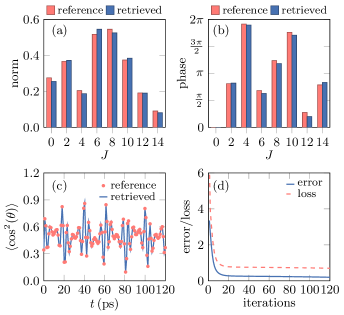
Figure 1: Comparison of reference (red) and reconstructed (blue) values of the norm (a) and phase (b) of $C_{J}$. The reconstruction is based on the $\braket{\cos^{2}(\theta)}(t)$ signal, including $3\%$ Gaussian noise, as shown in (c). Panel (d) illustrates the convergence of the target vector estimation error and the loss function, i.e. error with L2 regularization.

III.2 Thermal Ensembles

We now consider ensembles of molecules initially in mixed states including a large number of molecular rotational states. We consider two cases: (i) an ensemble of 3003 states $\ket{J,M}$ with even $J\leq 76$, where the initial populations are randomly drawn from a uniform distribution; and (ii) a thermal ensemble of molecules at room temperature. The reference signals for these ensembles are computed using the exact time propagation of each molecular state (up to $J=76$) participating in dynamics. The inferred probabilities are obtained using Eq. (15) based on RPWF with $N=30$, which leads to convergent results and is sufficient to recover the probability distribution. Figure 2 illustrates the efficiency of our approach applied to two different initial population distributions. We further illustrate the generality of our approach by the solid line in Fig. 2(b) showing the results for a thermal ensemble obtained without any information about relative population probabilities.

For a thermal ensemble, the population probability gradients [see Eq. (15)] can be extended by the chain rule to obtain the temperature gradient

$$\frac{dE}{dT}=\frac{dE}{d\bm{p}}\frac{d\bm{p}}{dT},$$ (16)

yielding a formalism for determining the temperature directly from an observed laser-induced alignment signal. The bars in Figure 2(b) illustrate the probabilities inferred for a Boltzmann distribution. The difference between the solid curve and the bars shows the improvement of the inference resulting from the inclusion of the temperature gradients. The convergence of inferred temperature for the thermal ensemble in Fig. 2(b) is illustrated in Fig. 3. The slower convergence of $T$ compared to the error is due to the exponential relation $p_{j}\sim\exp[-E/(kT)]$ where the small change in error corresponds to the large change in $T$ near the minimum. A related problem of inferring rotational temperature from an alignment signal was recently considered experimentally in Ref. Oppermann et al. (2012). The rotational temperature of molecules after impulsive excitation was obtained by least-squares fitting, limiting the application to cold gases ($<58$ K), with accuracy of $\approx 2-4\,\mathrm{K}$, likely limited by experimental noise. The present approach applies to a wider range of $T$ and allows for control of inference accuracy through the proper choice of L2 regularization, the number of iterations and $N$.

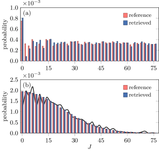
Figure 2: Comparison of reference (red) and reconstructed (blue) probabilities for: (a) – a mixture consisting of 3003 rotational states, $|JM\rangle$ with even $J\leq 76$ with random populations drawn from a uniform distribution; and (b) – a thermal ensemble of molecules with $T=300\,\mathrm{K}$. The reconstruction is based on $\braket{\cos^{2}(\theta)}(t)$ simulated using the RPWF approach. The solid curve in (b) is obtained without temperature gradients or any information on the relative population probabilities.

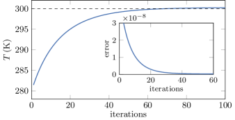
Figure 3: Convergence of the inferred temperature and the target vector estimation error (inset) for the $\braket{\cos^{2}(\theta)}(t)$ signal used for Fig. 2.

III.3 Pure State Excited by Two
Cross-Polarized Laser Pulses

We now consider a molecular ensemble excited by two delayed cross-polarized laser pulses: the first polarized along the $X$ axis and the second in the $XY$ plane at $45^{\circ}$ to the $X$ axis. Such an excitation induces molecular unidirectional rotation Fleischer et al. (2009); Lin et al. (2015); Mizuse et al. (2015), i.e. creates a wave packet with coherences between states with different $J$ and $M$. This significantly enlarges the corresponding density matrices and makes the inverse problem non-unique: a single alignment signal, $\braket{\cos^{2}(\theta)}$, is not sufficient to determine the probability amplitudes $C_{JM}$ for all $\ket{JM}$. The non-uniqueness is resolved by including multiple reference signals into the objective function in Eq. (5). We find that all $C_{JM}$ can be reconstructed if the reference signal includes simultaneously three observables: $\braket{\cos^{2}(\theta)}$, $\braket{\cos^{2}(\phi)}$ and $\braket{\sin^{2}(\theta)\sin(2\phi)}$. All of these observables can be probed either optically or using Coulomb explosion-based methods Renard et al. (2003); Faucher et al. (2011); Damari et al. (2016); Stapelfeldt and Seideman (2003); Koch et al. (2019); Karamatskos et al. (2019). Recently developed experimental techniques, such as the cold target recoil ion momentum spectroscopy (COLTRIMS) Dörner et al. (2000); Lin et al. (2015); Xu et al. (2020), allow one to probe these observables simultaneously. Figure 4 illustrates the norm and phase of each of the coefficients $C_{JM}$ inferred from a combination of these observables. The molecular state number refers to $\ket{JM}$ states ordered as $\ket{0,0},\,\ket{1,-1},\,\ket{1,0},\,\ket{1,1},\dots$

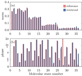
Figure 4: Comparison of reference (red) and reconstructed (blue) values of the norm (a) and phase (b) of $C_{JM}$ for the rotational wave packet produced by excitation of molecules initially in $\ket{J,M}=\ket{0,0}$ with two cross-polarized pulses. The molecular states are arranged in order of increasing $J$ and, for a given $J$, in order of increasing $M$. The wave-packet reconstruction is based on a combination of three signals: $\braket{\cos^{2}(\theta)}$, $\braket{\cos^{2}(\phi)}$ and $\braket{\sin^{2}(\theta)\sin(2\phi)}$ used simultaneously. Notice that the phase difference for molecular state 28 appears to be large as a consequence of constraining the phase to the interval $[0,2\pi)$.

III.4 Simultaneous Reconstruction

Finally, we consider a problem of simultaneous reconstruction of the Hamiltonian parameters ($\alpha$ and $P$) and the populations of a mixed state from a time-dependent alignment signal following a single-pulse excitation. We treat the molecular moment of inertia $I$ and the preparation field parameter $P$ in a linearly polarized (along $Z$ axis) laser pulse as unknown variables and supplement the gradients to include the derivatives with respect to $P$ and $I$. We write the derivatives in Eq. (9) as

$$\frac{\partial\bm{\psi_{j}}}{\partial P}=\frac{\partial\bm{V}(P)}{\partial P}\bm{\chi_{j}},$$ (17)

where $\bm{\chi}_{j}$ is a vector of $\langle\phi_{n}|\chi_{j}\rangle$. In addition, we express

$$\frac{\partial{\mathcal{O}}_{j}}{\partial I}=\frac{\partial{\mathcal{O}}_{j}}{\partial\bm{h}}\frac{\partial\bm{h}}{\partial I},$$ (18)

where $\bm{h}$ is a vector of eigenenergies, $h_{J}=J(J+1)/(2I)$. The first term can be explicitly written as

$$\frac{\partial{{\mathcal{O}}}_{j}}{\partial\bm{h}}=(it)\bm{u}^{\ast\top}\bm{A}_{j}\bm{u}-(it)\bm{u}^{\top}\bm{A}_{j}^{\top}\bm{u}^{\ast},$$ (19)

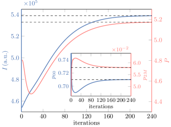
Figure 5: Convergence of the inferred field parameter $P$ and molecular moment of inertia $I$, using $\langle\cos^{2}\theta\rangle(t)$. The inset shows the convergence of the probabilities of $\ket{J=0,M_{J}=0}$, $\ket{2,-2}$, $\ket{2,-1}$, $\ket{2,0}$, $\ket{2,1}$ and $\ket{2,2}$ in the initial mixed state. The dashed lines show the reference values to be inferred.

where $\bm{u}$ is a vector of $\exp(ih_{J}t)$, $\bm{A}_{j}=\bm{S}_{j}^{\dagger}\bm{{\cal O}}\bm{S}_{j}$ and $\bm{S}_{j}$ is a diagonal matrix of $\langle\phi_{n}|\psi_{j}\rangle$. The second term is given by $\partial h_{J}/\partial I=-J(J+1)/(2I^{2})$. We apply Eqs. (9)–(11), and (17)–(19) to evaluate the gradient with respect to $P,\,I,\,p_{j}$, which are used in projected gradient descent. We consider an alignment signal $\braket{\cos^{2}(\theta)}(t)$ produced by exciting molecules with $I=539010\,\mathrm{a.u.}$ in a mixture of $J=0$ and $J=2$ states by linearly polarized pulse with $P=5.174$ yielding wave packets including rotational states with $J\leq 10$. Figure 5 illustrates the convergence of $I$, $P$ and the probabilities in the initial mixed state to the corresponding inferred values. Notice that all $\ket{2,M}$ states are equally populated initially.

IV Conclusion

In summary, we have shown that for a time-independent Hamiltonian $\hat{H}$ with spectrum parametrized by $\alpha$ and quantum states prepared by $\hat{V}(P)$ over finite time, it is possible to obtain closed-form expressions for the gradients of the distance between calculated and observed time-dependent signal with respect to $\alpha$, $P$ and the elements of the system density matrix. These gradients can be used in projected gradient descent to infer $\alpha$, $P$ and the density matrix from dynamical observables, such as molecular alignment or orientation. We have shown that this approach can be combined with random phase wave function approximation, yielding closed-form expressions for gradients that can be used to infer population distributions spanning a large number of molecular states from averaged time-dependent observables. We have illustrated that the temperature of a molecular gas at ambient conditions can be determined optically by probing time-dependence of alignment. This demonstrates a new way of probing molecular distributions in applications requiring remote sensing and opens new possibilities for solving inverse quantum problems with averaged dynamical observables.

We note that several important questions remain unanswered by this study. While our calculations demonstrate that some density matrices can be reconstructed with several simultaneously measured observables, we believe that the minimum number of observables required for the reconstruction of the full density matrix is generally not known. Refs. Jamiołkowski (1983, 2004) provided a formula for the minimum number of observables based on the degeneracy of the time evolution operator. In particular, it was suggested that a non-degenerate system requires $d$ observables, where $d$ is the dimension of the Hilbert space. However, this clearly contradicts our results in Sect. III.1 and the results in Refs. Hasegawa and Ohshima (2008); He et al. (2019); Karamatskos et al. (2019); Ueno et al. (2021). Further examination is required to investigate what determines the minimum amount of observable information, both in terms of the number of observables and the duration of the time-dependent signals, for the reconstruction of molecular density matrices, including the relationship between the number of observables, symmetries and parameters of the state-preparation fields. This question is particularly relevant for extensions of the present approach to include vibrational and electronic degrees of freedom.

Appendix: Derivative of Complex Quadratic Form

Consider $f(\bm{x})=\bm{x}^{\dagger}\bm{U}\bm{x}$, where $\bm{x}$ is a complex valued column vector and $\bm{U}$ is a Hermitian matrix:

$$\!f(\bm{x})=\sum_{i,j=1}^{n}x_{i}u_{ij}x_{j}=\sum_{i=1}^{n}\Big{[}u_{ii}x_{i}^{2}+\sum_{j\neq i}x_{i}u_{ij}x_{j}\Big{]},$$ (20)

where $x_{i}$ are the elements of $x$ and $u_{ij}$ are the elements of $U$. By writing $x_{i}=a_{i}+ib_{i}$, we recast Eq. (20) as

$$\begin{aligned} f(\bm{x})=\sum_{i=1}^{n}&\left[\vphantom{\sum_{i=1}^{n}}u_{ii}(a_{i}^{2}+b_{i}^{2})\right.+\\ &\left.\sum_{j\neq i}u_{ij}(a_{i}a_{j}+b_{i}b_{j}+ia_{i}b_{j}-ib_{i}a_{j})\right].\qquad\qquad\end{aligned}$$ (21)

A partial derivative with respect to $a_{k}$ is

$$\begin{aligned} \frac{\partial f}{\partial a_{k}}=&\quad 2u_{kk}a_{k}+\sum_{j\neq k}u_{kj}(a_{j}+ib_{j})+\sum_{i\neq k}u_{ik}(a_{i}-ib_{i})\\ =&\quad u_{kk}(a_{k}+ib_{k})+u_{kk}(a_{k}-ib_{k})\\ &\quad+\sum_{j\neq k}u_{kj}(a_{j}+ib_{j})+\sum_{i\neq k}u_{ik}(a_{i}-ib_{i})\\ =&\quad\sum_{j=1}^{n}u_{kj}(a_{j}+ib_{j})+\sum_{i=1}^{n}u_{ik}(a_{i}-ib_{i}),\end{aligned}$$ (22)

which yields

$$\nabla_{\bm{a}}f(\bm{x})=\left[\frac{\partial f}{\partial a_{k}}\right]=\bm{U}\bm{x}+\bm{U}^{\top}\bm{x}^{*}.$$ (23)

Similarly,

$$\frac{\partial f}{\partial b_{k}}=-i\sum_{j=1}^{n}u_{kj}(a_{j}+ib_{j})+i\sum_{i=1}^{n}u_{ik}(a_{j}-ib_{j}),$$ (24)

yielding

$$\nabla_{\bm{b}}f(\bm{x})=\left[\frac{\partial f}{\partial b_{k}}\right]=i\bm{U}^{\top}\bm{x}^{*}-i\bm{U}\bm{x}.$$ (25)

References

- Mouritzen and Mølmer (2006) A. S. Mouritzen and K. Mølmer, Quantum state tomography of molecular rotation, J. Chem. Phys. 124, 244311 (2006).
- Mandelshtam and Taylor (1997a) V. A. Mandelshtam and H. S. Taylor, Harmonic inversion of time signals and its applications, J. Chem. Phys. 107, 6756 (1997a).
- Avisar and Tannor (2011) D. Avisar and D. J. Tannor, Complete reconstruction of the wave function of a reacting molecule by four-wave mixing spectroscopy, Phys. Rev. Lett. 106, 170405 (2011).
- Hasegawa and Ohshima (2008) H. Hasegawa and Y. Ohshima, Quantum State Reconstruction of a Rotational Wave Packet Created by a Nonresonant Intense Femtosecond Laser Field, Phys. Rev. Lett. 101, 053002 (2008).
- He et al. (2019) X. He, S. Schmohl, and H.-D. Wiemhöfer, Direct Observation and Suppression Effect of Lithium Dendrite Growth for Polyphosphazene Based Polymer Electrolytes in Lithium Metal Cells, ChemElectroChem 6, 1166 (2019).
- Karamatskos et al. (2019) E. T. Karamatskos, S. Raabe, T. Mullins, A. Trabattoni, P. Stammer, G. Goldsztejn, R. R. Johansen, K. Długołecki, H. Stapelfeldt, M. J. J. Vrakking, S. Trippel, A. Rouzée, and J. Küpper, Molecular movie of ultrafast coherent rotational dynamics of OCS, Nat. Comm. 10, 3364 (2019).
- Ueno et al. (2021) K. Ueno, K. Mizuse, and Y. Ohshima, Quantum-state reconstruction of unidirectional molecular rotations, Phys. Rev. A 103, 053104 (2021).
- Mandelshtam and Taylor (1997b) V. A. Mandelshtam and H. S. Taylor, A low-storage filter diagonalization method for quantum eigenenergy calculation or for spectral analysis of time signals, J. Chem. Phys. 106, 5085 (1997b).
- Mandelshtam and Taylor (1997c) V. A. Mandelshtam and H. S. Taylor, Spectral analysis of time correlation function for a dissipative dynamical system using filter diagonalization: Application to calculation of unimolecular decay rates, Phys. Rev. Lett. 78, 3274 (1997c).
- Judson and Rabitz (1992) R. S. Judson and H. Rabitz, Teaching lasers to control molecules, Phys. Rev. Lett. 68, 1500 (1992).
- Peirce et al. (1988) A. P. Peirce, M. A. Dahleh, and H. Rabitz, Optimal control of quantum-mechanical systems: Existence, numerical approximation, and applications, Phys. Rev. A 37, 4950 (1988).
- N. Zakhariev and M. Chabanov (1997) B. N. Zakhariev and V. M. Chabanov, New situation in quantum mechanics (wonderful potentials from the inverse problem), Inverse Probl. 13, R47 (1997).
- Leroy and Bernstein (1970) R. J. Leroy and R. B. Bernstein, Dissociation Energy and Long‐Range Potential of Diatomic Molecules from Vibrational Spacings of Higher Levels, J. Chem. Phys. 52, 3869 (1970).
- Pashov et al. (2000) A. Pashov, W. Jastrzebski, and P. Kowalczyk, Construction of potential curves for diatomic molecular states by the IPA method, Comp. Phys. Comm. 128, 622 (2000).
- Kirschner and Watson (1973) S. M. Kirschner and J. K. Watson, RKR potentials and semiclassical centrifugal constants of diatomic molecules, J. Mol. Spectrosc. 47, 234 (1973).
- Vargas-Hernández et al. (2019) R. A. Vargas-Hernández, Y. Guan, D. H. Zhang, and R. V. Krems, Bayesian optimization for the inverse scattering problem in quantum reaction dynamics, New J. Phys. 21, 022001 (2019).
- Deng et al. (2020) Z. Deng, I. Tutunnikov, I. Sh. Averbukh, M. Thachuk, and R. V. Krems, Bayesian optimization for inverse problems in time-dependent quantum dynamics, J. Chem. Phys. 153, 164111 (2020).
- Palao and Kosloff (2003) J. P. Palao and R. Kosloff, Optimal control theory for unitary transformations, Phys. Rev. A 68, 062308 (2003).
- Beck (2014) A. Beck, Introduction to nonlinear optimization: Theory, algorithms, and applications with MATLAB (SIAM, 2014).
- Gelman and Kosloff (2003) D. Gelman and R. Kosloff, Simulating dissipative phenomena with a random phase thermal wavefunctions, high temperature application of the Surrogate Hamiltonian approach, Chem. Phys. Lett. 381, 129 (2003).
- Nest and Kosloff (2007) M. Nest and R. Kosloff, Quantum dynamical treatment of inelastic scattering of atoms at a surface at finite temperature: The random phase thermal wave function approach, J. Chem. Phys. 127, 134711 (2007).
- Kallush and Fleischer (2015) S. Kallush and S. Fleischer, Orientation dynamics of asymmetric rotors using random phase wave functions, Phys. Rev. A 91, 063420 (2015).
- Zare (1988) R. Zare, Angular momentum: understanding spatial aspects in chemistry and physics (Wiley, New York, 1988).
- V. Krems (2018) R. V. Krems, Molecules in Electromagnetic Fields: From Ultracold Physics to Controlled Chemistry (John Wiley & Sons, 2018).
- Stapelfeldt and Seideman (2003) H. Stapelfeldt and T. Seideman, Colloquium: Aligning molecules with strong laser pulses, Rev. Mod. Phys. 75, 543 (2003).
- Fleischer et al. (2012) S. Fleischer, Y. Khodorkovsky, E. Gershnabel, Y. Prior, and I. Sh. Averbukh, Molecular Alignment Induced by Ultrashort Laser Pulses and Its Impact on Molecular Motion, Isr. J. Chem. 52, 414 (2012).
- Koch et al. (2019) C. P. Koch, M. Lemeshko, and D. Sugny, Quantum control of molecular rotation, Rev. Mod. Phys. 91, 035005 (2019).
- Fleischer et al. (2009) S. Fleischer, Y. Khodorkovsky, Y. Prior, and I. Sh. Averbukh, Controlling the sense of molecular rotation, New J. Phys. 11, 105039 (2009).
- Leibscher et al. (2004) M. Leibscher, I. Sh. Averbukh, and H. Rabitz, Enhanced molecular alignment by short laser pulses, Phys. Rev. A 69, 013402 (2004).
- Trevor Hastie (2009) J. F. Trevor Hastie, Robert Tibshirani, The Elements of Statistical Learning: Data Mining, Inference, and Prediction (Springer, 2009).
- Oppermann et al. (2012) M. Oppermann, S. J. Weber, and J. P. Marangos, Characterising and optimising impulsive molecular alignment in mixed gas samples, Phys. Chem. Chem. Phys. 14, 9785 (2012).
- Lin et al. (2015) K. Lin, Q. Song, X. Gong, Q. Ji, H. Pan, J. Ding, H. Zeng, and J. Wu, Visualizing molecular unidirectional rotation, Phys. Rev. A 92, 013410 (2015).
- Mizuse et al. (2015) K. Mizuse, K. Kitano, H. Hasegawa, and Y. Ohshima, Quantum unidirectional rotation directly imaged with molecules, Sci. Adv. 1, e1400185 (2015).
- Renard et al. (2003) V. Renard, M. Renard, S. Guérin, Y. T. Pashayan, B. Lavorel, O. Faucher, and H. R. Jauslin, Postpulse Molecular Alignment Measured by a Weak Field Polarization Technique, Phys. Rev. Lett. 90, 153601 (2003).
- Faucher et al. (2011) O. Faucher, B. Lavorel, E. Hertz, and F. Chaussard, Optically Probed Laser-Induced Field-Free Molecular Alignment, in Progress in Ultrafast Intense Laser Science VII, edited by K. Yamanouchi, D. Charalambidis, and D. Normand (Springer Berlin Heidelberg, Berlin, Heidelberg, 2011) pp. 79–108.
- Damari et al. (2016) R. Damari, S. Kallush, and S. Fleischer, Rotational Control of Asymmetric Molecules: Dipole- versus Polarizability-Driven Rotational Dynamics, Phys. Rev. Lett. 117, 103001 (2016).
- Dörner et al. (2000) R. Dörner, V. Mergel, O. Jagutzki, L. Spielberger, J. Ullrich, R. Moshammer, and H. Schmidt-Böcking, Cold Target Recoil Ion Momentum Spectroscopy: a “momentum microscope” to view atomic collision dynamics, Phys. Rep 330, 95 (2000).
- Xu et al. (2020) L. Xu, I. Tutunnikov, L. Zhou, K. Lin, J. Qiang, P. Lu, Y. Prior, I. Sh. Averbukh, and J. Wu, Echoes in unidirectionally rotating molecules, Phys. Rev. A 102, 043116 (2020).
- Jamiołkowski (1983) A. Jamiołkowski, Minimal number of operators for observability of N-level quantum systems, Int. J. Theor. Phys. 22, 369 (1983).
- Jamiołkowski (2004) A. Jamiołkowski, On a stroboscopic approach to quantum tomography of qudits governed by gaussian semigroups, Open Syst. Inf. Dyn. 11, 63 (2004).