Distinguishing Primordial Magnetic Fields from Inflationary Tensor Perturbations in the Cosmic Microwave Background

Abstract

A claimed detection of cosmological tensor perturbations from inflation via B-mode polarization of the cosmic microwave background requires distinguishing other possible B-mode sources. One such potential source of confusion is primordial magnetic fields. For sufficiently low-amplitude B-mode signals, the microwave background temperature and polarization power spectra from power-law tensor perturbations and from a power-law primordial magnetic field are indistinguishable. However, we show that such a magnetic field will induce a small-scale Faraday rotation which is detectable using four-point statistics analogous to gravitational lensing of the microwave background. The Faraday rotation signal will distinguish a magnetic-field induced B-mode polarization signal from tensor perturbations for effective tensor-scalar ratios larger than 0.001, detectable in upcoming polarization experiments.

I Introduction

One of the primary goals of the next-generation of cosmic microwave background (CMB) experiments is to detect the primordial B-mode polarization signal from the tensor perturbations generated by inflation. A detection of this signal would be compelling evidence of inflation and help determine the physical mechanism of inflation. While early-universe inflation generically predicts the production of metric tensor perturbations with a nearly scale-invariant spectrum via quantum fluctuations in the gravitational field, the amplitude of the tensor spectrum can vary greatly between plausible inflation models.

The current best constraint on the tensor-to-scalar ratio is $r<0.056$ at $95\%$ confidence level through a combined analysis of Planck and BICEP2 (Hansen et al., 2018). The next generation of large-angle CMB polarization experiments. including the Simons Observertory (Ade et al., 2019), BICEP3 (Grayson et al., 2016), LiteBIRD (Hazumi et al., 2019), and CMB-S4 (Abazajian et al., 2016) will have the sensitivity and frequency range to reduce this bound to $r=10^{-3}$ or below. However, the tensor perturbations from inflation are not the only source of B-mode polarization in the CMB. Foregrounds and lensing, in particular, both are known to contribute to B-mode polarization. Even regions of the sky with expected low galactic foregrounds still have polarized foregrounds which are substantially larger than current upper limits on any primordial B-mode polarization component (Ade et al., 2015; Planck Collaboration et al., 2016; Ade et al., 2018). In order to separate foregrounds from cosmological polarization signals, the coming generation of large-angle B-mode experiments (BICEP3, Simons Observatory, LiteBIRD) will measure in many frequency bands, and test the spatial isotropy and gaussianity of any signal.

We also have known for a long time that the lensing B-mode signal has a low-$\ell$ contribution whose power spectrum can be mistaken for or confused with a low-amplitude primordial signal (Knox and Song, 2002). B-mode polarization from lensing has been detected in cross-correlation by SPT (Hanson et al., 2013) and ACT (van Engelen et al., 2015). We have made great progress at measuring lensing signals through their non-Gaussian 4-point signature (see, e.g., (Hu and Okamoto, 2002)), and now reconstruct maps of the lensing deflection potential with data from ACT (Darwish et al., 2020), SPT (SPT Collaboration (2013), Holder, G. P. et al.), and Planck (Planck Collaboration et al., 2020). In principle, this can be done with very high precision, given clean enough maps with low enough noise (see, e.g., (Simard et al., 2015; Seljak and Hirata, 2004)). But in practice there is a limit to how well low-$\ell$ lensing can be reconstructed due to having imperfect data with non-zero noise. For example, although detecting a signal with $r\sim 10^{-6}$ is theoretically achievable in the absence of any systematic errors, sky cuts, and foregrounds Seljak and Hirata (2004), realistic forecasts that include such effects generally predict a much lower sensitivity at the level of $\sigma(r)\sim 10^{-3}$ (Alonso et al., 2017).

Foregrounds and lensing are the two most important confusion signals for primordial B-mode polarization, and detailed studies and modeling of those are well in hand (see (Kamionkowski and Kovetz, 2016) for a review). What else could confuse us? Perhaps the next most-likely signal would be from a primordial magnetic field. Such concern has previously been brought up in, e.g., Refs. (Brown, 2010; Pogosian and Zucca, 2018), and discussed in Ref. (Renzi et al., 2018). The extent to which we can distinguish the two signals, given imperfect data with non-zero noise, motivates this paper.

Magnetic fields are ubiquitous in the universe today, with typical strengths of a few microgauss in galaxies and galaxy clusters (see, e.g., Ref. (Widrow, 2002; Durrer and Neronov, 2013; Kahniashvili et al., 2018) for reviews). Furthermore, evidence from the non-observation of the inverse Compton cascade $\gamma$-rays from the TeV blazars (Neronov and Vovk, 2010) suggests that magnetic fields are present in the intergalactic medium, with a lower limit of around $10^{-7}$ nG on megaparsec scales. However, the physical origin of the cosmic magnetic field remains poorly understood. One intriguing possibility is that cosmic magnetic fields are present before structure formation and are produced in the very early universe such as during inflation (Turner and Widrow, 1988) or during a phase transition (Vachaspati, 1991). Magnetic fields that are present before the decoupling of CMB photons are generally known as primordial magnetic fields.

If present, a primordial magnetic field impacts both the ionization history of the universe and structure formation, leaving imprints on the CMB and the matter power spectrum (Shaw and Lewis, 2010). In particular, primordial magnetic fields source scalar, vector, and tensor metric perturbations, and influence baryon physics through the Lorentz force. In addition, primordial magnetic field also introduces a net rotation of the linear polarization of the CMB photons through an effect known as Faraday rotation, which leaves an observable frequency-dependent signal in the CMB polarization pattern (Kosowsky and Loeb, 1996; Kosowsky et al., 2005).

The amplitude of the comoving magnetic field $B_{0}$ present today is constrained to be no more than a few nG (see, e.g., (Zucca et al., 2017; Ade et al., 2016)). However, it has been previously shown that a magnetic field with mean amplitude of around 1 nG and a power-law power spectrum can generate a CMB B-mode power spectrum similar to that of an inflationary tensor-mode signal with tensor-scalar ratio $r\simeq 0.004$ (Renzi et al., 2018). This is roughly the limiting tensor amplitude which will be detected by upcoming CMB experiments. Hence, a lack of knowledge of the primordial magnetic field may potentially lead us to a wrong conclusion if a B-mode polarization signal were to be detected by upcoming CMB experiments.

In this work we aim to review and re-evaluate, with particular focus on the upcoming CMB experiments, the potential degeneracy between a B-mode signal from a primordial magnetic field model and that from primordial gravitational waves. In particular, we evaluate the degeneracy for different tensor-to-scalar ratios $r$, in the context of experimental configurations that model the capabilities of upcoming CMB experiments. We also investigate the extent to which we can break the degeneracy with Faraday rotation from the magnetic field, at both the power spectrum level and the map level. In particular, as we shall show in Sec. V, quadratic estimation of Faraday rotation at 90 GHz gives a much more significant detection of magnetic fields than the power spectrum for a given map noise and resolution; for a tensor-mode signal at the level of $r=10^{-3}$, Faraday rotation clearly breaks the power spectrum degeneracy between tensor perturbations and magnetic fields.

This paper is organized as follows. In Sec. II, we review the basics of the primordial magnetic field. In Sec. III, we summarize the primordial magnetic field contributions to the CMB power spectrum and evaluate the potential confusion with the tensor-mode signal from inflation. In Sec. IV, we briefly review the physics of Faraday rotation from primordial magnetic field and discuss to what extent this effect allows us to break the degeneracy between primordial magnetic field and primordial tensor-mode signals. In Sec. V, we summarize the reconstruction of Faraday rotation through quadratic estimators and then discuss to what extent it helps us break the degeneracy. Finally, we discuss our results and conclude in Sec. VI.

II Primordial Magnetic Field

II.1 Statistics of stochastic magnetic fields

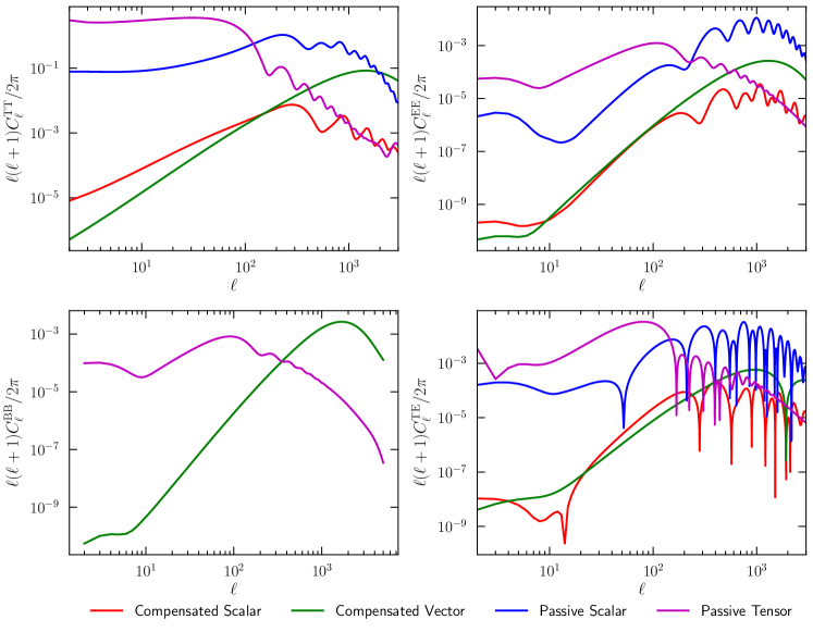
Figure 1: Contributions of different magnetic modes on the CMB power spectra (in units of $\mu$K²) from a stochastic background of primordial magnetic field with $\rm B_{1{\rm Mpc}}=1~{}{\rm nG}$, $\log_{10}\tau_{B}/\tau_{\nu}=17$, and $n_{B}=-2.9$ (nearly scale-invariant) generated using MagCAMB.

We consider a stochastic background of magnetic fields generated prior to recombination and shall assume that the magnetic field is weak enough to be treated as a perturbation to the mean energy density of the universe. As the universe is highly conductive prior to recombination, so any electric field quickly dissipates. On scales larger than the horizon, the magnetic field is effectively “frozen in” due to the negligible magnetic diffusion on cosmological scales. Hence, the conservation of magnetic flux gives the scaling relation $B^{i}(x^{j},\tau)=B^{i}(x^{j})/a(\tau)^{2}$, with $a$ the scale factor, $\tau$ the conformal time, and $x^{j}$ the comoving coordinates. We shall also assume that the stochastic background of magnetic fields follows the statistics of a Gaussian random field, and the energy density of magnetic fields, which scales quadratically with the magnetic field strength ($\propto B^{2}$), follows chi-square statistics. In Fourier space, the statistics of the magnetic field can be completely described by its 2-point correlations

$$\langle B_{i}^{*}(\mathbf{k})B_{j}(\mathbf{k}^{\prime})\rangle=(2\pi)^{3}\delta^{(3)}(\mathbf{k}-\mathbf{k}^{\prime})[P_{ij}P_{B}(k)+i\epsilon_{ijl}\hat{k}_{l}P_{H}(k)],$$ (1)

where $P_{ij}\equiv\delta_{ij}-\hat{k}_{i}\hat{k}_{j}$ is a projection operator onto the transverse plane to $\hat{k}$ such that $P_{ij}k^{j}=0$, and $\epsilon_{ijl}$ is the total anti-symmetric tensor. Here $P_{H}$ and $P_{B}$ refer to the helical and non-helical part of the magnetic field power spectrum, respectively. For the interests of simplicity we shall assume that the helical magnetic field component vanishes, though we should note that helical magnetic field is predicted by some proposed magnetogenesis scenarios (see, e.g., (Semikoz and Sokoloff, 2005; Campanelli and Giannotti, 2005)).

We assume that the power spectrum of magnetic field follows a power law with a cut-off scale $k_{D}$, given by

$$P_{B}=A_{B}k^{n_{B}},\>\>\>k\leq k_{D},$$ (2)

which vanishes for $k>k_{D}$. The dissipation scale $k_{D}$ reflects the suppression of magnetic field due to radiation viscosity on small scales. $A_{B}$ and $n_{B}$ denote the amplitude and spectral index of magnetic field power spectrum, respectively, both of which depend on the specific magnetogensis scenerio. In particular, an inflationary magnetogenesis model prefers a scale-invariant spectrum with a spectral index $n_{B}\approx 3$, while a causally-generated magnetic field in the post-inflationary epoch prefers a spectrum with $n_{B}\geq 2$ (Pogosian and Zucca, 2018).

The assumption that the magnetic field is “frozen-in” and follows a power law with a cut-off scale $k_{D}$ is only an approximation. Magnetohydrodynamic simulations (e.g., (Brandenburg et al., 1996; Banerjee and Jedamzik, 2003; Kahniashvili et al., 2016)) have shown that magnetic fields tend to source turbulence on scales smaller than the horizon. However, such an effect is expected to have negligible impact on the results in this paper as it affects mostly the small-scale magnetic fields, whereas, as we shall discuss in Sec. III, only the large-scale magnetic modes are degenerate with a primordial tensor mode signal. Thus we neglect subhorizon plasma dynamics.

In addition, following a common convention in the literature, we smooth the magnetic field with a Gaussian kernel $f_{\lambda}(x)=N\exp{(-x^{2}/2\lambda^{2})}$ on a comoving scale $\lambda$. The magnetic field fluctuation on the comoving scale $\lambda$ can then be characterized by

$$B_{\lambda}^{2}\equiv\langle\mathbf{B}_{\lambda}(\mathbf{x})\cdot\mathbf{B}_{\lambda}(\mathbf{x})\rangle=\frac{1}{\pi^{2}}\int_{0}^{\infty}dk~{}k^{2}e^{-k^{2}\lambda^{2}}P_{B}(k),$$ (3)

which relates to the power spectrum amplitude $A_{B}$ by

$$A_{B}=\frac{(2\pi)^{n_{B}+5}B_{\lambda}^{2}}{2\Gamma(\frac{n_{B}+3}{2})k_{\lambda}^{n_{B}+3}}.$$ (4)

The damping scale $k_{D}$ can also be approximated as (Mack et al., 2002),

$$\begin{split}k_{D}&=(5.5\times 10^{4})^{\frac{1}{n_{B}+5}}\left(\frac{B_{\lambda}}{1\,{\rm nG}}\right)^{-\frac{2}{n_{B}+5}}\left(\frac{2\pi}{\lambda/{\rm Mpc}}\right)^{\frac{n_{B}+3}{n_{B}+5}}\\ &\times h^{\frac{1}{n_{B}+5}}\left(\frac{\Omega_{b}h^{2}}{0.022}\right)^{\frac{1}{n_{B}+5}}|_{\lambda=1{\rm Mpc}}~{}{\rm Mpc}^{-1},\end{split}$$ (5)

with $h$ the reduced Hubble parameter defined as $h\equiv H_{0}/100$ km s^-1 Mpc^-1.

II.2 Magnetic Perturbations

Consider a particular realization of a stochastic magnetic field, with the magnitude of the field at $x$ and conformal time $\tau$ given by $B^{i}({\mathbf{x}},\tau)$. Its energy-momentum tensor can be written as

$$\begin{split}T^{0}{}_{0}&=-\frac{1}{8\pi a^{4}}B^{2}(\mathbf{x}),\\ T^{0}{}_{i}&=T^{i}{}_{0}=0,\\ T^{i}{}_{j}&=\frac{1}{4\pi a^{4}}\left[\frac{1}{2}B^{2}(\mathbf{x})\delta^{i}{}_{j}-B^{i}(\mathbf{x})B_{j}(\mathbf{x})\right],\end{split}$$ (6)

where we have used the “freeze-in” condition $B^{i}(\mathbf{x},\tau)=B^{i}(\mathbf{x})/a(\tau)^{2}$. Since $\rho_{B}\equiv T^{0}{}_{0}\propto a^{-4}$ scales the same way as photon energy density, one can reparametrize the magnetic field perturbation relative to the photon density $\rho_{\gamma}$ and pressure $p_{\gamma}$ as (Shaw and Lewis, 2010)

$$\begin{split}T^{0}{}_{0}&=-\rho_{\gamma}\Delta_{B},\\ T^{i}{}_{j}&=p_{\gamma}(\Delta_{B}\delta^{i}_{j}+\Pi^{i}{}_{Bj}),\\ \end{split}$$ (7)

where $\Delta_{B}$ denotes the scalar perturbations sourced by magnetic fields relative to the radiation energy density, and $\Pi^{i}{}_{Bj}$ denotes the anisotropic stress from magnetic fields which can be further decomposed into scalar, vector, and tensor type perturbations.

Initial conditions of magnetically-induced perturbation modes can be decomposed into three types: (1) compensated (Giovannini, 2004; Finelli et al., 2008), (2) passive (Lewis, 2004; Shaw and Lewis, 2010), and (3) inflationary (Bonvin et al., 2013). In particular, compensated magnetic modes arise when the magnetic contributions to the metric perturbations are compensated by fluid modes to the leading order on super-horizon scales. It includes the contributions from magnetic field after neutrino decoupling, and is finite in the $\tau\rightarrow 0$ limit. The passive magnetic modes, on the other hand, account for the magnetic contribution prior to neutrino decoupling. In this period, the universe is dominated by a tightly-coupled radiative fluid which prevents any anisotropic stress from developing. Without neutrino free-streaming, the magnetic field acts as the only source of anisotropic stress, leading to a logarithmically growing mode (Lewis, 2004). This mode survives neutrino decoupling as a constant offset on the amplitude of the non-magnetic mode. Inflationary magnetic modes, as another type of initial condition, depend on the specific generation mechanism (Bonvin et al., 2013), and is therefore not considered in this paper in order to maintain generality of our results to different magnetic field models.

From this physical picture it is apparent that the size of the perturbations from magnetic fields depends on the epoch of their generation relative to the epoch of neutrino decoupling, as can be parametrized by $\log_{10}(\tau_{\nu}/\tau_{B})$, with $\tau_{\nu}$ the neutrino decoupling time and $\tau_{B}$ the magnetic field generation time. Though the exact number for this quantity remains unknown and can be model-dependent, we shall assume $\log_{10}(\tau_{\nu}/\tau_{B})=17$ for simplicity, following Ref. (Ade et al., 2016). This is, nevertheless, without a loss of generality, as $\tau_{\nu}/\tau_{B}$ can be degenerate with the amplitude of the perturbations (e.g., $B_{\lambda}$ or $A_{B}$) (Shaw and Lewis, 2010). In addition, the magnetic field also introduces a Lorentz force acting on the baryons in the primordial plasma. It effectively augments the pressure perturbations of the baryon-photon fluid which prevent photons and baryons from falling into their gravitational wells. This effect is analogous to a change in baryon energy density which affects the sound speed of the baryon-photon fluid and changes their acoustic oscillations (Adams et al., 1996; Kahniashvili and Ratra, 2006; Kunze, 2011).

III Impacts on CMB power spectra

A primordial magnetic field influences CMB anisotropies through both its metric perturbations and the Lorentz force, and generates perturbations of scalar, vector, and tensor types. We make use of the publicly available code MagCAMB (Zucca et al., 2017) which extends the Boltzmann code CAMB (Lewis et al., 2000) to include the effects of a primordial magnetic field discussed in Sec. II. In Fig. 1 we show an example set of CMB power spectra that are sourced by a stochastic primordial magnetic field with $B_{1{\rm Mpc}}=1$ nG and a nearly scale-invariant spectrum ($n_{B}=-2.9$). Contributions from different magnetic modes are plotted in different colors, from which one observes that the passive tensor-mode signal in $C_{\ell}^{\rm BB}$ has significant power at $\ell\lesssim 100$ resembling that of an inflationary tensor-mode signal and hence may pose a possible source of confusion. On the other hand, the compensated vector-mode contribution dominates at $\ell\gtrsim 1000$ in both $C_{\ell}^{\rm TT}$ and $C_{\ell}^{\rm BB}$ which is not degenerate with the inflationary tensor-mode signal. Hence, this vector-mode perturbation from primordial magnetic field gives us a potential handle to break the degeneracy.

To evaluate the extent of the confusion for upcoming CMB experiments, we simulate different sets of CMB power spectra using CAMB with the standard $\Lambda$CDM model and the Planck best-fit cosmological parameters as our fiducial model Planck Collaboration et al. (2018), while varying the tensor-to-scalar ratio $r$ to reflect different science targets, with the spectral index $n_{T}$ fixed by the slow-roll inflation consistency relation $n_{T}=-r/8$. We consider several toy-model full-sky microwave background experiments specified by angular resolution and map sensitivity. In addition, we simulate the observed power spectra for each experiment with an idealized noise model given by

$$N_{\ell}=w^{-1}\exp\left(\ell(\ell+1)\theta^{2}/8\ln 2\right),$$ (8)

where $w^{-1/2}\equiv\sqrt{4\pi\sigma_{\rm pix}^{2}/N_{\rm pix}}$ denotes the expected noise level of an experiment, with $\sigma_{\rm pix}$ the per-pixel noise level, $N_{\rm pix}$ the total number of pixels, and $\theta$ the full-width-half-minimum (FWHM) size of a Gaussian telescope beam. We also assume that the polarization and temperature noise are related simply by $(\sigma^{\rm P}_{\rm pix})^{2}=2(\sigma^{\rm T}_{\rm pix})^{2}$.

In Tab. 1 we list the toy-model experiments considered in this work. In particular, Expt A and B approximate the capabilities of the Simons Observatory Large Aperture Telescope (SO LAT) and Small Aperture Telescope (SO SAT), respectively. Expt C1 represents a combined constraint with both of these experiments. Expt C2 represents the capability of the anticipated CMB-S4 experiment, while C3 is the limit of a noiseless CMB map so that the power spectrum uncertainty is due entirely to cosmic variance.

Name	Beam [arcmin]	Noise [$\mu$K arcmin]	$\ell_{\rm min}$	$\ell_{\rm max}$	$f_{\rm sky}$
A	17	2	30	1000	0.1
B	1.4	6	30	3000	0.4
C1	17	2	30	1000	0.1
	1.4	6	30	3000	0.4
C2	17	1	30	1000	0.1
	1.4	2	30	3000	0.4
C3	17	0	30	1000	0.1
	1.4	0	30	3000	0.4

Table 1: Different sets of experimental parameters considered in this paper. Expt A represents a ground-based small-aperture telescope, while Expt B represents a ground-based large-aperture telescope. C1, C2, and C3 represent a combination of Expt A and B at various noise levels.

We compute Markov Chain Monte Carlo (MCMC) model fitting to find the best-fit cosmologies for two competing models: (1) a model with a non-zero tensor-to-scalar ratio $r$ but no primordial magnetic field contribution ($\Lambda$CDM+r hereafter); (2) a model with $r=0$ but non-zero primordial magnetic field contribution ($\Lambda$CDM+PMF hereafter). The Markov Chain varies the standard cosmological parameters, plus either the tensor-scalar ratio or the primordial magnetic field amplitude and power spectrum index (see Appendix A for more details on the MCMC model fitting and example results from the Markov Chains). The log-likelihood for a given model is taken as (Hamimeche and Lewis, 2008)

$$\begin{split}-2\ln\mathcal{L}\left(\left\{\widehat{\mathbf{C}}_{\ell}\right\}|\{\mathbf{C}_{\ell}\}\right)=&\sum_{l}(2l+1)\bigg{\{}{\rm Tr}\left[\widehat{\mathbf{C}}_{\ell}\mathbf{C}_{\ell}^{-1}\right]\\ &-\ln\left|\widehat{\mathbf{C}}_{\ell}\mathbf{C}_{\ell}^{-1}\right|-3\bigg{\}},\end{split}$$ (9)

where $\mathbf{C}_{\ell}$ contains the theory power spectra given by

$$\mathbf{C}_{\ell}\equiv\begin{pmatrix}C_{\ell}^{\rm TT}&C_{\ell}^{\rm TE}&0\\ C_{\ell}^{\rm TE}&C_{\ell}^{\rm EE}&0\\ 0&0&C_{\ell}^{\rm BB}\\ \end{pmatrix},$$ (10)

and $\widehat{\mathbf{C}}_{\ell}$ contains the observed power spectra given by

$$\widehat{\mathbf{C}}_{\ell}\equiv\frac{1}{2\ell+1}\sum_{m}{\bm{a}}_{\ell m}{\bm{a}}_{\ell m}^{\dagger},$$ (11)

with ${\bm{a}}_{\ell m}\equiv(a_{\ell m}^{\rm T}~{}~{}a_{\ell m}^{\rm E}~{}~{}a_{\ell m}^{\rm B})^{T}$. Note that the full set of power spectra, $C_{\ell}^{\rm TT}$, $C_{\ell}^{\rm EE}$, $C_{\ell}^{\rm BB}$, and $C_{\ell}^{\rm TE}$ are used in the model-fitting.

Specifically, the simulated power spectrum is generated with the $\Lambda$CDM+r model, which we then fit with a $\Lambda$CDM+PMF model to find degenerate magnetic field models in terms of CMB power spectra. Although in theory the expected power spectra from the two competing models are not completely degenerate due to, for instance, the vector-mode signal from the primordial magnetic field, in practice the difference may not be detectable at a given experimental noise level, especially when $\rm B_{1{\rm Mpc}}\lesssim 1$ nG. By computing the $\Delta\chi^{2}$ between the two best-fit models, we evaluate the extent of the degeneracy between the $\Lambda$CDM+r model and the $\Lambda$CDM+PMF model at various $r$ targets and experiment sensitivities as listed in Tab. 1.

III.1 Fiducial cosmology with $r=0.01$

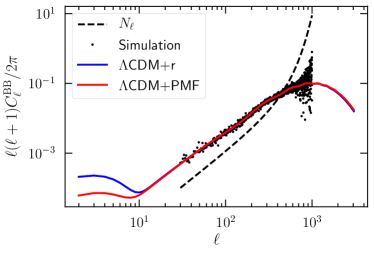
Figure 2: Best-fit $C_{\ell}^{\rm BB}$ power spectra (in units of $\mu$K²) for the $\Lambda$CDM+r (blue) and $\Lambda$CDM+PMF (red) models, to an underlying tensor cosmology with $r=0.01$ and map noise Expt A in Tab. 1. The black dots represent the simulated data after removing noise model UNCLEAR, and the black dashed line represents the noise model.

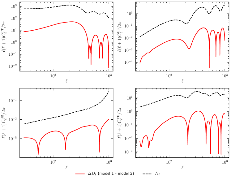
Figure 3: Difference of the two best-fit CMB power spectra in Fig. 2 is shown by the red solid line. The black dashed line shows the analytic covariance of the simulated power spectrum.

We first consider a target of $r=0.01$ which is one of the primary goals of the upcoming CMB experiments such as the Simons Observatory (SO) Ade et al. (2019). In particular, SO will have two separate instruments for measuring different angular scales of the CMB power spectrum: a large-aperture telescope (LAT) which mainly focuses on small-angle CMB anisotropies, and a small-aperture telescope (SAT) which mainly focuses on the large-angle CMB anisotropies. As the tensor-mode signal from inflation is expected to show up predominantly in the large angular scales, it is the main target of the SO SAT experiment.

Suppose that we live in a universe well described by a $\Lambda$CDM+r model with $r=0.01$, and we measure the CMB power spectrum with an SO SAT-like experiment, specified as Expt A in Tab. 1. We simulate the observed CMB power spectra for Expt A between angular scales of $\ell_{\rm min}=30$ and $\ell_{\rm max}=3000$, with a sky fraction of $f_{\rm sky}=0.3$, to account for the effect of partial sky coverage from a ground-based experiment.

We then fit the simulated data with both the $\Lambda$CDM+r and the $\Lambda$CDM+PMF models. The resulting B-mode polariation power spectra $C_{\ell}^{\rm BB}$ for the two best-fit models are shown in Fig. 2, compared to the simulated data. It shows that the two competing models can be highly degenerate over the angular scales probed by the simulated experiment (Expt A; $30\lesssim\ell\lesssim 3000$), with a difference much smaller than the variance of the observed data. To be more specific, one can model the variance of the observed data as Kamionkowski et al. (1997)

$$\sigma^{2}\left(C_{\ell}\right)=\frac{2}{(2\ell+1)f_{\mathrm{sky}}}\left(C_{\ell}+N_{\ell}\right)^{2},$$ (12)

and compare it to the difference between the two sets of best-fit power spectra, as shown in Fig. 3. The difference in the best-fit power spectra is around $2$ orders of magnitude below the expected variance of the observed power spectrum, indicating that breaking the degeneracy between the two models is impossible without additional information. The corresponding difference in $\chi^{2}$ between these two best-fit models is $\Delta\chi^{2}\simeq 0.1$

The degeneracy between the two models is not too surprising because on large angular scales ($\ell\lesssim 100$) the passive tensor mode dominates over the other contributions from the primordial magnetic field, and the passive tensor mode is mathematically equivalent to the inflationary tensor-mode signal; the degeneracy is unavoidable if one observes only at the large angular scales. On the other hand, one does see noticeable difference between the two models at $\ell\lesssim 10$, indicating that the two models are not completely degenerate on all angular scales. This is expected because in the small angular scales ($\ell\gtrsim 1000$), the compensated vector mode signal from a primordial magnetic field starts to dominate over the other magnetic modes in the $C_{\ell}^{\rm BB}$ power spectrum. This difference in the small scales gets minimized by the best-fit model, leading to the difference seen at $\ell\lesssim 10$. This also implies that the small-scale CMB anisotropies contain crucial information that helps break the degeneracy between $r=0.01$ in tensor perturbations and a primordial magnetic field.

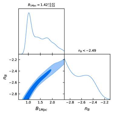
Figure 4: Joint posterior distributions for the $\Lambda$CDM+PMF model parameters after fitting the simulated data (generated with a $\Lambda$CDM+r model with $r=0.01$) to a $\Lambda$CDM+PMF model.

In Fig. 4 we show the posterior distributions of the magnetic field parameters ($\rm B_{1{\rm Mpc}}$ and $n_{B}$) from the $\Lambda$CDM+PMF model fitting an inflationary tensor perturbation at $r=0.01$. Specifically, we obtain a best-fit primordial magnetic field model with $\rm B_{1{\rm Mpc}}=1.42^{+0.42}_{-0.54}$ nG at 68% confidence level, on par with the observational constraints set by Planck in 2015 Ade et al. (2016). We also note that a nearly scale-invariant spectrum, with a spectral index of $n_{B}<-2.49$, is preferred by the simulated data, which we find a generic feature of the $\Lambda$CDM+PMF models degenerate to $\Lambda$CDM+r. An apparent degeneracy between the amplitude of the magnetic field $\rm B_{1{\rm Mpc}}$ and the magnetic spectral index $n_{B}$ can also be seen. This is because as $n_{B}$ increases, the power spectrum of primordial magnetic field tilts toward the smaller scales, leading to less power in the large scale modes which Expt A (or an SO SAT-like experiment) is sensitive to, and thus the loss of power gets compensated by a stronger magnetic field.

Now suppose that one obtains additional observations from a large-aperture telescope like the SO LAT, specified as Expt B in Tab. 1, which strongly constrains the small-scale CMB anisotropies. One can then combine its constraining power with Expt A to jointly constrain the primordial magnetic field on both small and large angular scales. For simplicity, we simulate the observed power spectra of the combined constraint by simulating two separate experiments with the same underlying CMB realization and combining them trivially by using the experiment that gives the lowest variance at each $\ell$ to avoid mode double counting.

In Fig. 5, we show how the joint posterior distribution of the magnetic field parameters ($B_{1{\rm Mpc}}$ and $n_{B}$) changes after we include the data from Expt B to the constraint. The degeneracy between $n_{B}$ and $\rm B_{1{\rm Mpc}}$ is broken when the additional observations from Expt B (or an SO LAT-like experiment) are included which tightly constrains the small scale modes of the primordial magnetic field. The joint constraint leads to a much tighter allowed parameter space, shown as the red contour, favoring a primordial magnetic field with $\rm B_{1{\rm Mpc}}\sim 1$ nG and a scale-invariant spectrum. We find a $\Delta\chi^{2}\simeq-2.5$ between the best-fit $\Lambda$CDM+r model and the $\Lambda$CDM+PMF model, showing a stronger preference to the $\Lambda$CDM+r model. This improvement in $\Delta\chi^{2}$ is driven by the stronger constraining power in the small angular scales on the compensated vector-mode signal from primordial magnetic field which dominates at small angular scales ($\ell\gtrsim 1000$) and has no degenerate signal in $\Lambda$CDM+r. This indicates that if an apparent primordial B-mode signal is detected at an amplitude of around $r=0.01$, a joint constraint using both large and small angular scale measurements is a promising approach to rule out a degenerate $\Lambda$CDM+PMF model.

Figure 5: Joint posterior distributions of the magnetic field parameters after fitting a $\Lambda$CDM+PMF model to the simulated CMB power spectra with a fiducial model of inflationary tensor modes with $r=0.01$. The red contour shows the posterior distribution obtained from Expt A only, while the blue contour shows the posterior distribution as a result of a joint constraint from Expt A and Expt B, as specified in Tab. 1. The levels indicate the 68% and 95% confidence levels, respectively.

III.2 Lower $r$ targets

In addition to the fiducial model with $r=0.01$ discussed in the preceding section, we also repeat the study in Sec. III.1 for different targets of $r$ ranging from $0.001$ to $0.010$, and compute $\Delta\chi^{2}$ between the two best-fit models for each set of the simulations of a given $r$. In particular, we consider three sets of combined observations specified as C1, C2, C3 in Tab. 1. C1 represents the set of observations considered in Sec. III.1 as a joint constraint of Experiment A and B, C2 represents a similar set of experiments with lower noise levels, and C3 represents the same set of experiments in a noise-less limit.

The results of model-fitting show that the degenerate $\Lambda$CDM+PMF models generally favor a nearly scale-invariant spectrum ($n_{B}\simeq-2.9$) with $\rm B_{1{\rm Mpc}}\lesssim 0.8$ nG, which is below the current observational limits. Fig. 6 shows how the amplitude of the magnetic field in the degenerate $\Lambda$CDM+PMF model varies with $r$. This is useful as it gives us a reference to what range of the primordial magnetic field parameter space is of interests to a particular $r$ target. It shows that, in general, one needs only worry about scale-invariant primordial magnetic field models with $\rm B_{1{\rm Mpc}}\gtrsim 0.5$ nG when targetting $r\gtrsim 0.001$. The results also show that, as the noise level of the experiment improves, more magnetic field parameter space will be strongly constrained, thus reducing the allowed amplitude of the degenerate primordial magnetic field model.

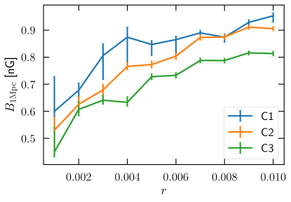
Figure 6: The magnitudes of magnetic field ($\rm B_{1{\rm Mpc}}$) that fits the simulated data at different target $r$ for Expt C1, C2, C3 specified in Tab. 1. The error bars indicate the 68% confidence interval for the marginal posterior distribution.

In Fig. 7 we show how $\Delta\chi^{2}$ between the two best-fit models changes as we vary $r$ for each of the three sets of simulated observations. As a reference, we compare the $\Delta\chi^{2}$ with a 95% confidence level of a $\chi^{2}$ distribution with one degree of freedom ($\Delta\chi^{2}=-3.841$) since the two competing models differ by one degree of freedom. We note that the results feature an apparent trend particularly for Expt C2, and also some fluctuations particularly at $r\lesssim 0.004$. This is likely due to a combination of realization-induced randomness and a poor convergence of some of the MCMC chains. Nevertheless, combined with Fig. 6, one sees a generic trend in the reduction of $\rm B_{1{\rm Mpc}}$ and the increasing of $\Delta\chi^{2}$ as noise level reduces or as $r$ is lowered, which matches our expectations. Thus our results are likely sensible approximations of the future performances, which are sufficient for our discussion here. In particular, one can see that the performance of Expt C1 in breaking the degeneracy between the two models quickly degrades as $r\lesssim 0.008$. With Expt C2 which has a much lower noise level similar to the targeting performance of the CMB-S4 experiments Abazajian et al. (2016), the situation is much improved as the degeneracy is effectively broken for any $r\gtrsim 0.004$. In the noise-less limit (C3), the degeneracy limit is pushed further down to $r\lesssim 0.002$. This implies that we will be cosmic variance limited to make a distinction between an inflationary tensor-mode signal and a primordial magnetic field signal below $r\lesssim 0.002$.

Note that our conclusions so far are based entirely on constraining primordial magnetic field through its effects on the CMB power spectra by means of metric perturbations and Lorentz force. However, this is not the only way one can constrain primordial magnetic field signals. In fact, primordial magnetic field also induces a Faraday rotation effect on the polarization of the CMB photons (Kosowsky et al., 2005), thus providing an additional means to constrain primordial magnetic field models. Hence, in the subsequent sections we will examine whether such effect can improve our ability to distinguish the two models.

IV B-Mode Polarization from Faraday Rotation

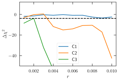
Figure 7: How $\Delta\chi^{2}$ varies with different targets of $r$. The three lines represent the three simulated set of observations specified in Tab. 1. The black dashed line shows a reference level of $\Delta\chi^{2}=-3.841$ which corresponds to the 95% confidence level for a $\chi^{2}$ distribution with one degree of freedom.

Another probe of primordial magnetic field is through the effect of Faraday rotation, in which the presence of magnetic field causes a net rotation of the linear polarization directions of the CMB photons along their path. The rotation angle $\alpha$ depends on the frequency of observation and the integrated electron density along the line of sight,

$$\alpha=\frac{3}{16\pi^{2}e}\lambda_{0}^{2}\int\dot{\tau}\tilde{\mathbf{B}}(\mathbf{x})\cdot d{\bm{l}},$$ (13)

where $\lambda_{0}$ is the observed wavelength, $\dot{\tau}\equiv n_{e}\sigma_{T}a$ is the differential optical depth proportional to the electron number density $n_{e}$, and $\tilde{\mathbf{B}}\equiv\mathbf{B}a^{2}$ is the comoving magnetic field. For a homogeneous magnetic field with a present amplitude of $\sim 1$ nG, the net rotation of the polarization angle is about a degree at 30 GHz, with the size of the effect scaling with frequency as $\alpha\propto v^{-2}$ (Kosowsky and Loeb, 1996). For a stochastic magnetic field with a power spectrum $P_{B}(k)$, the rotation field $\alpha(\mathbf{\hat{n}})$ is anisotropic with a 2-point correlation function given by Pogosian et al. (2011)

$$\begin{split}\langle\alpha(\hat{n})&\alpha(\hat{n}^{\prime})\rangle=\left(\frac{3\lambda_{0}^{2}}{16\pi^{2}e}\right)^{2}\int\frac{d^{3}k}{(2\pi)^{3}}P_{B}(k)\int d\eta\int d\eta^{\prime}\\ &\times\dot{\tau}(\eta)\dot{\tau}(\eta^{\prime})e^{-i\mathbf{k}\cdot\hat{n}\eta}e^{i\mathbf{k}\cdot\hat{n}^{\prime}\eta^{\prime}}[\hat{n}\cdot\hat{n}^{\prime}-(\hat{k}\cdot\hat{n})(\hat{k}\cdot\hat{n}^{\prime})],\end{split}$$ (14)

which can also be written as

$$\langle\alpha(\hat{n})\alpha(\hat{n}^{\prime})\rangle=\sum_{L}\frac{2L+1}{4\pi}C_{L}^{\alpha\alpha}P_{L}(\hat{n}\cdot\hat{n}^{\prime}),$$ (15)

with $P_{L}(x)$ the Legendre polynomials and $C_{L}^{\alpha\alpha}$ the rotational power spectrum. The rotational power spectrum follows as

$$C_{L}^{\alpha\alpha}=\left(\frac{3\lambda_{0}^{2}}{16\pi^{2}e}\right)^{2}\frac{2L(L+1)}{\pi}\int_{0}^{\infty}\frac{dk}{k}k^{3}P_{B}(k)T_{L}^{2}(k),$$ (16)

where we have defined a transfer function $T_{L}(k)$ as

$$T_{L}(k)\equiv\int_{0}^{k\Delta\eta}\frac{dx}{x}~{}\dot{\tau}(\eta_{0}-x/k)j_{L}(x).$$ (17)

Here $\eta_{0}$ is the conformal time today, $j_{L}(x)$ is the Spherical Bessel function, and $\Delta\eta\equiv\eta_{0}-\eta_{*}$ with $\eta_{*}$ corresponding to the conformal time at the maximum visibility. Eq. 16 provides the general expression for the rotational power spectrum generated by a primordial magnetic field model with a given $P_{B}(k)$.

The rotation field effectively turns E-mode polarization into B-mode polarization, leading to a B-mode power spectrum $C_{\ell}^{\rm BB}$ given by Pogosian et al. (2011)

$$\begin{split}C_{\ell}^{\rm BB}=&\sum_{\ell_{2}L}\frac{(2L+1)(2\ell_{2}+1)}{2\pi}C_{L}^{\rm\alpha\alpha}C_{\ell_{2}}^{\rm EE}\left(H_{\ell\ell_{2}}^{L}\right)^{2}\\ &~{}~{}~{}\times\left(1+(-1)^{L+\ell+\ell_{2}}\right),\end{split}$$ (18)

where $H_{\ell\ell_{2}}^{L}$ is defined through the Wigner 3j symbol (Wigner, 1993) as

$$H_{\ell\ell_{2}}^{L}\equiv\begin{pmatrix}\ell&L&\ell_{2}\\ 2&0&-2\end{pmatrix}.$$ (19)

Eq. 18 gives the expected signal in $C_{\ell}^{\rm BB}$ from an anisotropic rotation field $\alpha(\mathbf{\hat{n}})$ with a power spectrum $C_{L}^{\alpha\alpha}$, giving us an additional means to probe the primordial magnetic field model through the Faraday rotation effect.

IV.1 Faraday rotation from a scale-invariant primordial magnetic field

As discussed in Sec. III.1, primordial magnetic field models that generate potentially degenerate B-mode signals to the primordial gravitational wave are approximately scale-invariant. Hence we focus exclusively on the this class of primordial magnetic field models (with $n_{B}\simeq-2.9$) in this section. In addition, we make another simplifying assumption that the magnetic modes with scales smaller than the thickness of the last scattering surface contribute negligibly to the total Faraday rotation, so we only consider magnetic modes for $k\lesssim k_{D}$ with $k_{D}\simeq 2$ Mpc^-1. This assumption is motivated by the fact that the total Faraday rotation is dominated by the large-scale modes, as the rotation generated by magnetic modes with scales smaller than the thickness of the last scattering surface tends to cancel due to the Faraday depolarization effect Sokoloff et al. (1998).

With the assumptions above, the transfer function $T_{L}(k)$ defined in Eq. 17 can then be approximated as

$$T_{L}(k)\simeq\frac{j_{L}(k\eta_{0})}{k\eta_{0}},$$ (20)

where we have used the approximation that $\Delta\eta\approx\eta_{0}$ and the fact that the differential optical depth $\dot{\tau}$ is sharply peaked relative to the slowly varying magnetic field (as we have ignored the fast varying modes with scales smaller than the thickness of the last scattering surface) and integrates to $\simeq 1$ near the last scattering surface. The rotation power spectrum $C_{L}^{\rm\alpha\alpha}$ then becomes

$$\begin{split}C_{L}^{\alpha\alpha}&=\frac{9L(L+1)\lambda_{0}^{4}}{4(2\pi)^{5}e^{2}\eta_{0}^{3}}\int_{0}^{k_{D}}\mathrm{d}k~{}P_{B}(k)j_{L}^{2}(x)\\ &=\frac{9L(L+1)B_{\lambda}^{2}\nu_{0}^{-4}}{(4\pi)^{3}\Gamma\left(\frac{n_{B}+3}{2}\right)e^{2}}\left(\frac{\lambda}{\eta_{0}}\right)^{n_{B}+3}\int_{0}^{x_{D}}dx~{}x^{n_{B}}j_{L}^{2}(x),\end{split}$$ (21)

where $x_{D}\equiv k_{D}\eta_{0}$, $\nu_{0}$ is the observing frequency, and $\lambda=1$ Mpc is the length of the smoothing kernel. This result is consistent with that given in Ref. (Kosowsky et al., 2005). Specifically, we follow the same approximation as in Ref. (Kosowsky et al., 2005) that replaces $j_{L}^{2}(x)$ with $1/2x^{2}$ after the second zero of $j_{L}(x)$ in Eq. 21 to simplify the numerical integration of the fast oscillating functions. In Fig. 8 we show the rotation power spectrum of a primordial magnetic field with $\rm B_{1{\rm Mpc}}=1$ nG for different $n_{B}$, as calculated from Eq. 21. The results show that as the spectral index approaches $n_{B}\simeq-3$, the rotation spectrum approaches a scale-invariant limit as expected. The above derivations assume the CMB polarization is generated instantaneously in the beginning of recombination, which is not true. A full calculation also needs to consider that Faraday rotation occurs alongside with the generation of CMB polarization. This effect has been calculated in Ref. (Pogosian et al., 2011) and shown to result in difference small compared to our order of magnitude estimate here.

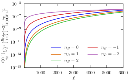
Figure 8: Rotation power spectrum for different magnetic spectral indices $n_{B}$ calculated using Eq. 21 with the Planck 2018 best-fit cosmology Planck Collaboration et al. (2018), $\nu_{0}=100$ GHz, and $\rm B_{1{\rm Mpc}}=1$ nG. The amplitude of the power spectrum scales with $\rm B_{1{\rm Mpc}}^{2}$ and $\nu_{0}^{-4}$.

With the rotational power spectrum $C_{\ell}^{\alpha\alpha}$, one can then estimate the expected $C_{\ell}^{\rm BB}$ power spectrum sourced by the rotation field using Eq. 18. In Fig. 9, we show the expected B-mode power spectrum sourced by a nearly scale-invariant primordial magnetic field with $n_{B}=-2.9$ and $\rm B_{1{\rm Mpc}}=1$ nG, observed at 100 GHz. The result shows two noticeable features: (1) Faraday rotation signal in $C_{\ell}^{\rm BB}$ peaks at small angular scales (at $\ell\sim 1000$), similar to the CMB lensing signal, with a significantly lower amplitude than CMB lensing; (2) Unlike the CMB lensing signal, the B-mode signal from the rotation field displays acoustic oscillations similar to those in CMB E-mode power spectrum. This is expected since, according to Eq. 18, the B-mode signal from the rotation field is effectively a convolution of the E-mode power spectrum $C_{\ell}^{\rm EE}$ with the rotation power spectrum $C_{\ell}^{\rm\alpha\alpha}$ in $\ell$-space. $C_{\ell}^{\rm\alpha\alpha}$ is scale invariant, so the variation with $\ell$ in the resulting $C_{\ell}^{\rm BB}$ is determined by that of $C_{\ell}^{\rm EE}$, thus reflecting the acoustic oscillations. This is a unique feature that allows distinguishing the rotation signal from the lensing signal in the $C_{\ell}^{\rm BB}$.

To project the performance of future CMB experiments in constraining the primordial magnetic field by measuring the Faraday rotation signal, we define the signal-to-noise ratio (SNR) as

$$\left(\frac{S}{N}\right)^{2}=\sum_{\ell}\frac{(2\ell+1)f_{\rm sky}\left(C_{\ell}^{\rm BB,FR}\right)^{2}}{2\left(C_{\ell}^{\rm BB,tot}+N_{\ell}^{\rm BB}\right)^{2}},$$ (22)

with $C_{\ell}^{\rm BB,FR}$ the expected B-mode signal from the Faraday rotation, and $C_{\ell}^{\rm BB,tot}$ the total B-mode signal that includes the contributions both the Faraday rotation signal and the CMB lensing signal. $N_{\ell}^{\rm BB}$ refers to the expected B-mode noise power spectrum from a given experiment as approximated by Eq. 8. The factor $f_{\rm sky}$ is added to approximate the effect of the partial sky coverage of a realistic experiment, in the form of a reduction in the number of available measurements and thus a reduction in the total SNR. In addition, we assume an observing frequency of 100 GHz for the subsequent discussion. Lower frequencies increase the rotation signal for a given magnetic field, but are also technically more difficult to attain comparable map sensitivity and resolution.

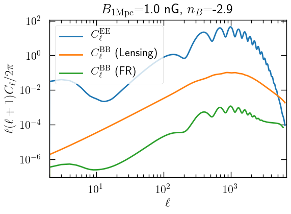
Figure 9: The green curve shows the B-mode signal (in units of $\mu$K²) generated by the Faraday rotation of a primordial magnetic field with $n_{B}=-2.9$ and $\rm B_{1{\rm Mpc}}=1$ nG at $\nu_{0}=100$ GHz. The orange curve shows the expected lensing signal and the blue curve shows the $C_{\ell}^{\rm EE}$ signal. Note that “FR” denotes Faraday rotation.

As the Faraday rotation signal is significant mainly on small angular scales, large-aperture experiments are most relevant to detecting such signal. Specifically, we consider Expt B as specified in Tab. 1 with different noise levels (6 $\mu$K arcmin, 2 $\mu$K arcmin, and 0 $\mu$K arcmin), and compute the SNR for each experiment for a scale-invariant primordial magnetic field with the amplitude $\rm B_{1{\rm Mpc}}$ varying from 0.1 nG to 1 nG. The resulting SNRs are presented in Fig. 10, which shows that for an SO LAT-like experiment with a noise level of 6 $\mu$K arcmin, the Faraday rotation signal is not detectable in the power spectrum, hence contributing negligible constraining power on the primordial magnetic field. In comparison, a CMB S4-like experiment with a noise level of 2 $\mu$K arcmin barely detects a primordial magnetic field with $\rm B_{1{\rm Mpc}}\gtrsim 0.9$ nG at SNR $\gtrsim 1$, while at the noiseless limit, one can detect a primordial magnetic field with $\rm B_{1{\rm Mpc}}\gtrsim 0.5$ nG with SNR $\gtrsim 1$, and $\rm B_{1{\rm Mpc}}\gtrsim 0.8$ nG with SNR $\gtrsim 3$. As concluded from Fig. 6, degenerate primordial magnetic field models of interest to the upcoming experiments generally have amplitudes $\rm B_{1{\rm Mpc}}$ ranging from $\sim 0.5-1$ nG, comparable to the detection limit of the noiseless case. This suggests that Faraday rotation in the B-mode power spectrum is unlikely a competitive constraint on the primordial magnetic field.

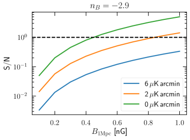
Figure 10: Signal-to-noise ratio for various $\rm B_{1{\rm Mpc}}$. The three different solid curves show the S/N curve for three experiments with various noise levels. The dashed curve indicates the threshold of $S/N=1$.

On the other hand, the above SNR estimates neglect the effect of delensing, which is a procedure to remove the CMB lensing signal from the B-mode power spectrum (see, e.g., (Smith et al., 2012)). As the CMB lensing signal is generally much larger than the Faraday rotation signal in $C_{\ell}^{\rm BB}$, being able to remove a significant portion of the lensing signal significantly reduces the total variance in the B-mode power spectrum, thus improving the SNR. To be more specific, we can denote the $C_{\ell}^{\rm BB,tot}$ in Eq. 22 as

$$C_{l}^{\rm BB,tot}=C_{l}^{\rm BB,CMB}+C_{l}^{\rm BB,FR}+A_{\rm delens}C_{\ell}^{\rm BB,lensing},$$ (23)

where $C_{l}^{\rm BB,CMB}$, $C_{\ell}^{\rm BB,FR}$, and $C_{\ell}^{\rm BB,lensing}$ denote the B-mode signal from the CMB, primordial magnetic field, and lensing, respectively, and $A_{\rm delens}$ denotes the residual fraction of delensing which characterizes the delensing efficiency. Optimistic estimates suggest that an SO-like experiment can achieve $A_{\rm delens}\sim 0.5$ with inputs from external datasets (Ade et al., 2019), and a CMB S4-like experiment with a noise level around 2 $\mu$K arcmin can achieve $A_{\rm delens}\sim 0.4$ Abazajian et al. (2016). If the B-mode power spectrum is signal dominated, delensing can improve the signal-to-noise ratio by a factor of $A_{\rm delens}^{-1}$, thus lowering the primordial magnetic field detection limit by a factor of $A_{\rm delens}^{-1/2}$.

V Rotational field reconstruction from primordial magnetic field

Faraday rotation acts as an effective rotation field $\alpha(\mathbf{\hat{n}})$ that rotates the CMB polarization field:

$${}_{\pm 2}A(\hat{\mathbf{n}})\equiv(Q\pm iU)(\hat{\mathbf{n}})=e^{\pm 2i\alpha(\hat{\mathbf{n}})}(\tilde{Q}\pm i\tilde{U})(\hat{\mathbf{n}}),$$ (24)

where $Q$ and $U$ refer to the Stoke parameters for the rotated polarization field and we use tilde to denote the unrotated polarization field. In the limit that $\alpha(\hat{\mathbf{n}})\ll 1$, $\delta_{\pm 2}A(\mathbf{\hat{n}})\simeq\pm 2i\alpha(\mathbf{\hat{n}}){}_{\pm 2}\tilde{A}(\mathbf{\hat{n}})$. Such rotation induces off-diagonal correlations between E-mode and B-mode polarization maps (Kamionkowski, 2009; Yadav et al., 2009) (see Appendix B for a derivation), given by

$$\langle E_{lm}B_{l^{\prime}m^{\prime}}^{*}\rangle_{\rm CMB}=~{}\sum_{LM}\alpha_{LM}\xi_{lml^{\prime}m^{\prime}}^{LM}f_{lLl^{\prime}}^{\rm EB},$$ (25)

with

$$f_{lLl^{\prime}}^{\rm EB}=2\epsilon_{lLl^{\prime}}[H_{l^{\prime}l}^{L}\tilde{C}_{l}^{\rm EE}-H_{ll^{\prime}}^{L}\tilde{C}_{l}^{\rm BB}],$$ (26)

$$\begin{split}\xi_{lml_{2}m_{2}}^{LM}\equiv(-1)^{m}&\sqrt{\frac{(2L+1)(2l_{2}+1)(2l+1)}{4\pi}}\\ &\qquad\times\begin{pmatrix}l&L&l_{2}\\ -m&M&m_{2}\end{pmatrix},\end{split}$$ (27)

and

$$\epsilon_{lLl_{2}}\equiv\frac{1+(-1)^{l+L+l_{2}}}{2}.$$ (28)

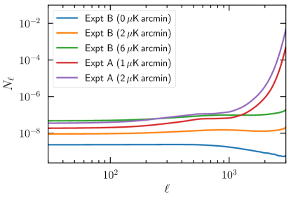
Figure 11: Gaussian noise covariance $N_{L}^{\rm EB}$ for experiments specified in Tab. 1 with varying noise levels.

The $\langle...\rangle_{\rm CMB}$ denotes that the average is to be taken over CMB realisations only. The coupling also allows one to reconstruct the rotation field $\alpha_{LM}$ with a quadratic estimator similar to the reconstruction of CMB lensing Hu and Okamoto (2002):

$$\hat{\alpha}_{LM}=A_{L}^{\rm EB}\sum_{ll^{\prime}}\sum_{mm^{\prime}}\xi_{lml^{\prime}m^{\prime}}^{LM}g_{ll^{\prime}}^{\rm EB}E_{lm}B_{l^{\prime}m^{\prime}}^{*},$$ (29)

with normalization factor $A_{L}$ defined as

$$\left(A_{L}^{\rm EB}\right)^{-1}=\sum_{ll^{\prime}}\frac{(2l+1)(2l^{\prime}+1)}{4\pi}g_{ll^{\prime}}^{\rm EB}f_{lLl^{\prime}}^{\rm EB},$$ (30)

ensuring the quadratic estimator is unbiased. The weights $g_{ll^{\prime}}^{\rm EB}$ can be chosen to minimize the total variance of the estimator $\langle\alpha_{LM}^{*}\alpha_{LM}\rangle$ with

$$g_{ll^{\prime}}^{\rm EB}=\frac{f_{lLl^{\prime}}^{\rm EB}}{C_{l}^{\rm EE}C_{l^{\prime}}^{\rm BB}},$$ (31)

The minimized variance of estimator, denoted as $N_{L}^{\rm EB}$, is related to the normalization factor as

$$N_{L}^{\rm EB}=A_{L}^{\rm EB}=\sum_{ll^{\prime}}\frac{(2l+1)(2l^{\prime}+1)}{4\pi}\frac{(f_{lLl^{\prime}}^{\rm EB})^{2}}{C_{l}^{\rm EE}C_{l^{\prime}}^{\rm BB}},$$ (32)

with $C_{l}^{\rm EE}$ and $C_{l^{\prime}}^{\rm BB}$ the observed E- and B-mode power spectrum, respectively. Here $N_{L}^{\rm EB}$ is a dimensionless quantity that characterizes the variance of the reconstructed rotation angle at each $L$.

In Fig. 11, we show the expected reconstruction noise $N_{L}^{EB}$ calculated using Eq. 32 for experiments considered previously in Tab. 1, and for a nearly scale invariant primordial magnetic field with varying amplitudes of $\rm B_{1{\rm Mpc}}$ and $n_{B}=-2.9$. In particular, we consider Expt A with noise levels of 2 $\mu$K arcmin and 1 $\mu$K arcmin, and Expt B with noise levels of 6 $\mu$K arcmin, 2 $\mu$K arcmin, and 0 $\mu$K arcmin. The results show that the large-aperture experiments have orders of magnitude lower reconstruction noise at $\ell\gtrsim 1000$, confirming our expectation that the small-scale CMB anisotropies have stronger constraining power on the Faraday rotation signal.

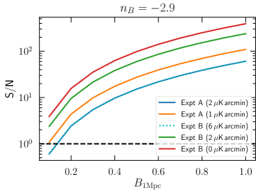
Figure 12: Signal-to-noise ratio expected for the quadratic estimator in a variety of experimental settings. The black dashed line represents S/N=1.

To forecast the expected performance of the quadratic estimator for future CMB experiments, we define the SNR as

$$(S/N)^{2}=\sum_{L=L_{\rm min}}^{L_{\rm max}}f_{\rm sky}\frac{2L+1}{2}\left(\frac{C_{L}^{\alpha\alpha}}{N_{L}^{EB}}\right)^{2},$$ (33)

where, similar to Sec. IV, we use $f_{\rm sky}$ to approximate the partial sky coverage. We also assume the observations are made at 100 GHz, which is the frequency channel expected to contribute the highest SNR.

In Fig. 12 we show the expected SNR for the same set of experiments considered previously. It shows that reconstructing a rotation field using the quadratic estimator approach results in an order of magnitude improvement in the SNR as compared to constraining its effects on the CMB B-mode power spectrum. This is consistent with the claims in (Mandal et al., 2022) and is unsurprising as the effect of a rotation field $\alpha$ on $C_{\ell}^{\rm BB}$ scales as $\alpha^{2}$, which is a second order effect, whereas its effect on the cross-correlation $\langle EB\rangle$ scales with $\alpha$ (see Eq. 25), which is a first order effect, thus giving a significantly improved SNR. The results also show that large-aperture experiments (Expt B) have better SNR in general as a result of the significantly lower reconstruction noise (as shown in Fig. 11). Specifically, a SO SAT-like experiment with a noise level of 2 $\mu$K arcmin gives comparable SNR to an SO LAT-like experiment with a noise level of 6 $\mu$K arcmin, both of which are capable of constraining primordial magnetic field models down to $\rm B_{1{\rm Mpc}}\gtrsim 0.3$ nG with $S/N\gtrsim 3$. CMB S4-like noise levels push down this limit to $\rm B_{1{\rm Mpc}}\gtrsim 0.1$ nG.

These calculations demonstrate that primordial magnetic field models which have B-mode power spectra degenerate with primordial tensor modes with $r>0.001$ will be strongly constrained by the rotation signal in small-scale anisotropies. As in Sec. IV, we have neglected the effect of delensing, which may further improve the primordial magnetic field constraint.

VI Discussion

We have investigated the following question: can primordial magnetic fields be distinguished from primordial gravitational waves as a source of B-mode polarization in the CMB power spectrum? Concerns over a possible degeneracy in the B-mode power spectrum signal have previously been raised (see, e.g., (Pogosian and Zucca, 2018; Renzi et al., 2018)). In this work we have confirmed with simulations that the answer is likely “no” if one utilizes only the information in the large-scale CMB anisotropies ($\ell\lesssim 1000$), as a primordial magnetic field also introduces large-scale B-mode signals by sourcing tensor-mode metric perturbations in a mathematically equivalent form to that of the primordial gravitational waves, thus generating a completely degenerate signal on large angular scales. However, as we have further demonstrated, after including small-scale CMB polarization anisotropies ($\ell\gtrsim 1000$), the answer becomes “yes” because of both the magnetic field’s vector-mode contribution to B-mode polarization on small scales, and especially due to Faraday rotation of E-mode polarization into B-mode. Upcoming high-sensitivity measurements of polarization at small scales will enable this distinction for any magnetic field which might be mistaken for a primordial tensor mode signal when using only large-angle B-mode polarization data. We have demonstrated this explicitly for tensor-mode amplitudes down to $r=10^{-3}$. For even smaller tensor-mode signals, at some point sufficient delensing techniques must be demonstrated. The amplitude at which lensing signals become an important consideration remains to be seen Cai et al. (in prep.).

Our analysis extends previous work (e.g., Refs. (Renzi et al., 2018)) in considering a wider class of magnetic field models and tensor-to-scalar ratio targets, and more importantly, also in explicitly identifying degenerate magnetic field models to a given tensor-mode signal using simulations and MCMC-based model-fitting. We also for the first time consider map-based Faraday rotation estimation as a way to break the degeneracy between tensor modes and magnetic fields. Our result provides a practical recipe to follow: should a potential tensor-mode signal be detected in the CMB B-mode power spectrum, one can identify degenerate magnetic field models from our analysis and look for its Faraday rotation signal. Upper limits on such a signal provides a clear route to ruling out a plausible contaminant to a tensor B-mode signal. Magnetic fields thus join gravitational lensing and galactic foregrounds as known B-mode contributors for which we possess clear methods of discriminating them from the hallmark signature of early-universe inflation.

VII Acknowledgments

We thank Daniel Boyanovsky for helpful comments on the manuscript. YG acknowledges the partial support of PITT PACC in the duration of this work. This research was supported in part by the University of Pittsburgh Center for Research Computing through the resources provided.

Appendix A MCMC

We perform MCMC-based model fitting using an ensemble sampler from emcee [Foreman-Mackey et al., 2013] with 50 walkers. We use with a mixed proposal function that makes stretch moves 95% of the time and Gaussian moves based on the fisher matrix 5% of the time. We find that the resulting MCMC chains generally converge well after 400 steps based on autocorrelation tests and adopt a fixed number of 400 steps for all subsequent MCMC runs. Specifically, for $\Lambda$CDM+r model, we adopt flat priors on $\omega_{b}$, $\omega_{\rm CDM}$, $H_{0}$, $n_{s}$, $A_{s}$, $r$, and a Gaussian prior on $\tau_{\rm reio}$ with $\tau_{\rm reio}=0.065\pm 0.015$. For the $\Lambda$CDM+PMF model, we use a flat prior on $\rm B_{1{\rm Mpc}}$ with $0\leq\rm B_{1{\rm Mpc}}\leq 2.5$ nG, and a flat prior on $n_{B}$ restricted to $-2.9\leq n_{B}\leq 0$.

In Fig. 13 and Fig. 14, we show the full set of posterior distributions for the $\Lambda$CDM+r and $\Lambda$CDM+PMF models respectively, when fitting the simulated observations from Expt A with a fiducial cosmology with non-zero tensor-to-scalar ratio, $r=0.01$. A burn-in ratio of 70% has been applied to obtain the posterior distributions.

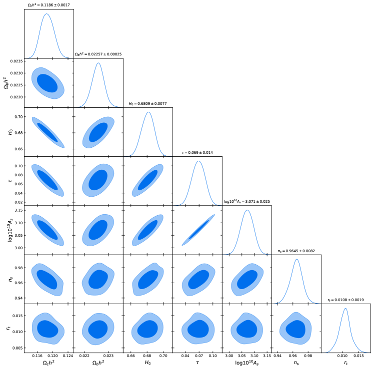
Figure 13: Best-fit $\Lambda$CDM+r cosmological parameters obtained for simulated data for Expt A with a fiducial cosmology with $r=0.010$.

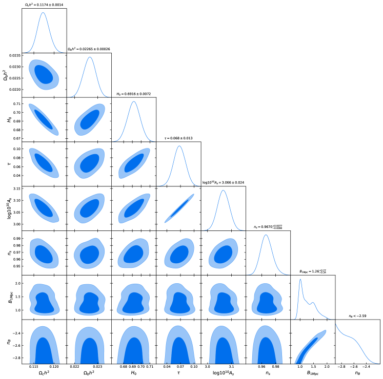
Figure 14: Best-fit $\Lambda$CDM+PMF cosmological parameters obtained for simulated data for Expt A with a fiducial cosmology with $r=0.010$.

Appendix B Quadratic estimator for polarization rotation

Faraday rotation acts as an effective rotation field $\alpha(\mathbf{\hat{n}})$ which rotates the CMB polarization maps, given by

$${}_{\pm 2}A(\hat{\mathbf{n}})\equiv(Q\pm iU)(\hat{\mathbf{n}})=e^{\pm 2i\alpha(\hat{\mathbf{n}})}(\tilde{Q}\pm i\tilde{U})(\hat{\mathbf{n}}),$$ (34)

where $Q$ and $U$ refer to the Stoke parameters for the rotated CMB photons. Approximating $\alpha$ as a small angle, the change in the polarization field due to rotation can be approximated as $\delta({}_{\pm 2}A(\mathbf{\hat{n}}))\simeq\pm 2i\alpha(\mathbf{\hat{n}}){}_{\pm 2}\tilde{A}(\mathbf{\hat{n}})$. In $lm$ space, the change in ${}_{\pm 2}A_{lm}$ is

$$\begin{split}\delta({}_{\pm 2}A_{lm})\simeq&\pm 2i\sum_{\rm LM}\sum_{l_{2}m_{2}}\alpha_{LM}{}_{\pm 2}A_{l_{2}m_{2}}\\ &\times\int d\hat{\mathbf{n}}~{}{}_{\pm 2}Y_{lm}^{*}(\hat{\mathbf{n}})Y_{LM}(\hat{\mathbf{n}}){}_{\pm 2}Y_{l_{2}m_{2}}(\hat{\mathbf{n}}),\end{split}$$ (35)

where ${}_{s}Y_{lm}$ denotes the spin-weighted spherical harmonics [Goldberg et al., 1967]. The integral can be performed with the formula

$$\begin{split}\int&d\hat{\mathbf{n}}_{s_{1}}Y_{l_{1}m_{1}}(\hat{\mathbf{n}})_{s_{2}}Y_{l_{2}m_{2}}(\hat{\mathbf{n}})_{s_{3}}Y_{l_{3}m_{3}}(\hat{\mathbf{n}})=\left[\frac{\prod_{i=1}^{3}2l_{i}+1}{4\pi}\right]^{1/2}\\ &\times\left(\begin{array}[]{ccc}j_{1}&j_{2}&j_{3}\\ m_{1}&m_{2}&m_{3}\end{array}\right)\left(\begin{array}[]{ccc}j_{1}&j_{2}&j_{3}\\ -s_{1}&-s_{2}&-s_{3}\end{array}\right),\end{split}$$ (36)

which gives

$$\delta({}_{\pm 2}A_{lm})\simeq\pm 2i\sum_{\rm LM}\sum_{l_{2}m_{2}}\alpha_{LM}{}_{\pm 2}A_{l_{2}m_{2}}\xi_{lml_{2}m_{2}}^{LM}{}_{\pm}H_{ll_{2}}^{L},$$ (37)

with

$$\xi_{lml_{2}m_{2}}^{LM}\equiv(-1)^{m}\sqrt{\frac{(2L+1)(2l_{2}+1)(2l+1)}{4\pi}}\begin{pmatrix}l&L&l_{2}\\ -m&M&m_{2}\end{pmatrix},$$ (38)

and

$${}_{\pm}H_{ll_{2}}^{L}\equiv\begin{pmatrix}l&L&l_{2}\\ \pm 2&0&\mp 2\end{pmatrix}=(-1)^{l+L+l_{2}}{}_{\mp}H_{ll_{2}}^{L}.$$ (39)

On the other hand, the polarization field ${}_{\pm 2}A_{lm}$ can be decomposed into the curl-free (E-mode) and the gradient-free (B-mode) components with

$$\begin{split}E_{lm}&=\frac{1}{2}\left({}_{+2}A_{lm}+{}_{-2}A_{lm}\right),\\ B_{lm}&=\frac{1}{2i}\left({}_{+2}A_{lm}-{}_{-2}A_{lm}\right).\\ \end{split}$$ (40)

This gives

$$\delta E_{lm}=-2i\sum_{LM}\sum_{l_{2}m_{2}}\alpha_{LM}\xi_{lml_{2}m_{2}}^{LM}H_{ll_{2}}^{L}\left(\beta_{lLl_{2}}\tilde{E}_{l_{2}m_{2}}+\epsilon_{lLl_{2}}\tilde{B}_{l_{2}m_{2}}\right),$$ (41)

and

$$\delta B_{lm}=2\sum_{LM}\sum_{l_{2}m_{2}}\alpha_{LM}\xi_{lml_{2}m_{2}}^{LM}H_{ll_{2}}^{L}\left(\epsilon_{lLl_{2}}\tilde{E}_{l_{2}m_{2}}-\beta_{lLl_{2}}\tilde{B}_{l_{2}m_{2}}\right),$$ (42)

where we have defined $H_{ll_{2}}^{L}\equiv{}_{+}H_{ll_{2}}^{L}$ and defined

$$\epsilon_{lLl_{2}} \equiv\frac{1+(-1)^{l+L+l_{2}}}{2},$$ (43)

$$\beta_{lLl_{2}} \equiv\frac{1-(-1)^{l+L+l_{2}}}{2}.$$

Eq. 41 and Eq. 42 describe the effect of Faraday rotation on the CMB E-mode and B-mode polarization maps, respectively, which effectively mixes the multipole moments of the two maps through rotation. This introduces couplings between the E-mode and B-mode maps at different $l$ which otherwise do not exist, given by

$$\langle E_{lm}B_{l^{\prime}m^{\prime}}^{*}\rangle_{\rm CMB}=~{}\sum_{LM}\alpha_{LM}\xi_{lml^{\prime}m^{\prime}}^{LM}f_{lLl^{\prime}}^{\rm EB},$$ (44)

with

$$f_{lLl^{\prime}}^{\rm EB}=2\epsilon_{lLl^{\prime}}[H_{l^{\prime}l}^{L}\tilde{C}_{l}^{\rm EE}-H_{ll^{\prime}}^{L}\tilde{C}_{l}^{\rm BB}].$$ (45)

The $\langle...\rangle_{\rm CMB}$ denotes that the average is to be taken over CMB realisations only. One can then define an unbiased quadratic estimator for rotation field as

$$\hat{\alpha}_{LM}=A_{L}^{\rm EB}\sum_{ll^{\prime}}\sum_{mm^{\prime}}\xi_{lml^{\prime}m^{\prime}}^{LM}g_{ll^{\prime}}^{\rm EB}E_{lm}B_{l^{\prime}m^{\prime}}^{*},$$ (46)

with the normalization factor to ensure the estimator is unbiased, given by

$$\left(A_{L}^{\rm EB}\right)^{-1}=\sum_{ll^{\prime}}\frac{(2l+1)(2l^{\prime}+1)}{4\pi}g_{ll^{\prime}}^{\rm EB}f_{lLl^{\prime}}^{\rm EB},$$ (47)

in doing so we have used

$$\sum_{mm^{\prime}}\xi_{lml^{\prime}m^{\prime}}^{LM}\xi_{lml^{\prime}m^{\prime}}^{L^{\prime}M^{\prime}}=\frac{(2l+1)(2l^{\prime}+1)}{4\pi}\delta_{LL^{\prime}}\delta_{MM^{\prime}}.$$ (48)

References

- Hansen et al. [2018] F K Hansen, D Herranz, E Hivon, D C Hooper, Z Huang, A H Jaffe, W C Jones, E Keihänen, R Keskitalo, K Kiiveri, J Kim, T S Kisner, N Krachmalnicoff, M Kunz, H Kurki-Suonio, G Lagache, J.-M Lamarre, A Lasenby, M Lattanzi, C R Lawrence, M Le Jeune, J Lesgourgues, F Levrier, A Lewis, M Liguori, D M White, A Zacchei, J P Zibin, A Zonca, and Fabio Finelli. Planck 2018 results. X. Constraints on inflation arXiv:1807.06211v1. J. A. Rubiño-Martín, 60:61, 2018.
- Ade et al. [2019] Peter Ade, James Aguirre, Zeeshan Ahmed, Simone Aiola, Aamir Ali, et al. The Simons Observatory: Science goals and forecasts. Journal of Cosmology and Astroparticle Physics, 2019(2), 2019. ISSN 14757516. doi: 10.1088/1475-7516/2019/02/056.
- Grayson et al. [2016] J. A. Grayson, P. A. R. Ade, Z. Ahmed, K. D. Alexander, M. Amiri, et al. BICEP3 performance overview and planned Keck Array upgrade. jul 2016. doi: 10.1117/12.2233894.
- Hazumi et al. [2019] M. Hazumi, P. A. R. Ade, Y. Akiba, D. Alonso, K. Arnold, et al. LiteBIRD: A Satellite for the Studies of B-Mode Polarization and Inflation from Cosmic Background Radiation Detection. Journal of Low Temperature Physics, 194(5-6):443–452, mar 2019. ISSN 0022-2291. doi: 10.1007/s10909-019-02150-5.
- Abazajian et al. [2016] Kevork N. Abazajian, Peter Adshead, Zeeshan Ahmed, Steven W. Allen, David Alonso, et al. CMB-S4 Science Book, First Edition. oct 2016.
- Ade et al. [2015] P.A.R. Ade, Z. Ahmed, R. W. Aikin, K. D. Alexander, D. Barkats, et al. BICEP2 / Keck Array V: Measurements of B-mode polarization at degree angular scales and 150 GHz by the Keck Array. Astrophysical Journal, 811(2), 2015. ISSN 15384357. doi: 10.1088/0004-637X/811/2/126.
- Planck Collaboration et al. [2016] Planck Collaboration, R. Adam, P. A. R. Ade, N. Aghanim, M. Arnaud, J. Aumont, C. Baccigalupi, A. J. Banday, R. B. Barreiro, J. G. Bartlett, and et al. Planck intermediate results. XXX. The angular power spectrum of polarized dust emission at intermediate and high Galactic latitudes. A&A, 586:A133, February 2016. doi: 10.1051/0004-6361/201425034.
- Ade et al. [2018] P. A. R. Ade, Z. Ahmed, R. W. Aikin, K. D. Alexander, et al. Constraints on primordial gravitational waves using , wmap, and new bicep2/ observations through the 2015 season. Phys. Rev. Lett., 121:221301, Nov 2018. doi: 10.1103/PhysRevLett.121.221301.
- Knox and Song [2002] Lloyd Knox and Yong-Seon Song. Limit on the Detectability of the Energy Scale of Inflation. Phys. Rev. Lett. , 89(1):011303, July 2002. doi: 10.1103/PhysRevLett.89.011303.
- Hanson et al. [2013] D. Hanson, S. Hoover, A. Crites, P. A. R. Ade, K. A. Aird, et al. Detection of B-Mode Polarization in the Cosmic Microwave Background with Data from the South Pole Telescope. Phys. Rev. Lett. , 111(14):141301, October 2013. doi: 10.1103/PhysRevLett.111.141301.
- van Engelen et al. [2015] Alexander van Engelen, Blake D. Sherwin, Neelima Sehgal, Graeme E. Addison, Rupert Allison, et al. The Atacama Cosmology Telescope: Lensing of CMB Temperature and Polarization Derived from Cosmic Infrared Background Cross-correlation. Astrophys. J. , 808(1):7, July 2015. doi: 10.1088/0004-637X/808/1/7.
- Hu and Okamoto [2002] Wayne Hu and Takemi Okamoto. Mass Reconstruction with Cosmic Microwave Background Polarization. The Astrophysical Journal, 574(2):566–574, 2002. ISSN 0004-637X. doi: 10.1086/341110.
- Darwish et al. [2020] Omar Darwish, Mathew S Madhavacheril, Blake Sherwin, et al. The Atacama Cosmology Telescope : A CMB lensing mass map over 2100 square degrees of sky and its cross-correlation with BOSS-CMASS galaxies. (January), 2020.
- SPT Collaboration (2013) [Holder, G. P. et al.] SPT Collaboration (Holder, G. P. et al.). A cosmic microwave background lensing mass map and its correlation with the cosmic infrared background. Astrophys. J. , 771:L16, 2013.
- Planck Collaboration et al. [2020] Planck Collaboration, N Aghanim, Y Akrami, M Ashdown, J Aumont, et al. Planck 2018 results. VIII. Gravitational lensing. 641:A8, sep 2020. doi: 10.1051/0004-6361/201833886.
- Simard et al. [2015] Gabrielle Simard, Duncan Hanson, and Gil Holder. Prospects for Delensing the Cosmic Microwave Background for Studying Inflation. Astrophys. J. , 807(2):166, July 2015. doi: 10.1088/0004-637X/807/2/166.
- Seljak and Hirata [2004] Uroš Seljak and Christopher M. Hirata. Gravitational lensing as a contaminant of the gravity wave signal in the CMB. Phys. Rev. D, 69(4):043005, February 2004. doi: 10.1103/PhysRevD.69.043005.
- Alonso et al. [2017] David Alonso, Joanna Dunkley, Ben Thorne, and Sigurd Næss. Simulated forecasts for primordial B -mode searches in ground-based experiments. Phys. Rev. D, 95(4):043504, February 2017. doi: 10.1103/PhysRevD.95.043504.
- Kamionkowski and Kovetz [2016] Marc Kamionkowski and Ely D. Kovetz. The Quest for B Modes from Inflationary Gravitational Waves. ARA&A, 54:227–269, September 2016. doi: 10.1146/annurev-astro-081915-023433.
- Brown [2010] Iain A. Brown. Concerning the statistics of cosmic magnetism. arXiv e-prints, art. arXiv:1005.2982, May 2010.
- Pogosian and Zucca [2018] Levon Pogosian and Alex Zucca. Searching for primordial magnetic fields with CMB B-modes, 2018. ISSN 13616382.
- Renzi et al. [2018] Fabrizio Renzi, Giovanni Cabass, Eleonora Di Valentino, Alessandro Melchiorri, and Luca Pagano. The impact of primordial magnetic fields on future cmb bounds on inflationary gravitational waves. Journal of Cosmology and Astroparticle Physics, 2018(08):038–038, Aug 2018. ISSN 1475-7516. doi: 10.1088/1475-7516/2018/08/038.
- Widrow [2002] Lawrence M. Widrow. Origin of galactic and extragalactic magnetic fields. Reviews of Modern Physics, 74(3):775–823, 2002. ISSN 00346861. doi: 10.1103/RevModPhys.74.775.
- Durrer and Neronov [2013] Ruth Durrer and Andrii Neronov. Cosmological magnetic fields: their generation, evolution and observation. A&A Rv, 21:62, June 2013. doi: 10.1007/s00159-013-0062-7.
- Kahniashvili et al. [2018] Tina Kahniashvili, Axel Brandenburg, Arthur Kosowsky, Sayan Mandal, and Alberto Roper Pol. Magnetism in the Early Universe, 2018.
- Neronov and Vovk [2010] Andrii Neronov and Ievgen Vovk. Evidence for Strong Extragalactic Magnetic Fields from Fermi Observations of TeV Blazars. Science, 328(5974):73, Apr 2010. doi: 10.1126/science.1184192.
- Turner and Widrow [1988] Michael S. Turner and Lawrence M. Widrow. Inflation-produced, large-scale magnetic fields. Phys. Rev. D, 37:2743–2754, May 1988. doi: 10.1103/PhysRevD.37.2743.
- Vachaspati [1991] T. Vachaspati. Magnetic fields from cosmological phase transitions. Phys. Lett., B265:258–261, 1991. doi: 10.1016/0370-2693(91)90051-Q.
- Shaw and Lewis [2010] J. Richard Shaw and Antony Lewis. Massive neutrinos and magnetic fields in the early universe. Phys. Rev. D, 81:043517, 2010.
- Kosowsky and Loeb [1996] Arthur Kosowsky and Abraham Loeb. Faraday Rotation of Microwave Background Polarization by a Primordial Magnetic Field. The Astrophysical Journal, 469:1, 1996. ISSN 0004-637X. doi: 10.1086/177751.
- Kosowsky et al. [2005] Arthur Kosowsky, Tina Kahniashvili, George Lavrelashvili, and Bharat Ratra. Faraday rotation of the cosmic microwave background polarization by a stochastic magnetic field. Physical Review D, 71(4), Feb 2005. ISSN 1550-2368. doi: 10.1103/physrevd.71.043006.
- Zucca et al. [2017] Alex Zucca, Yun Li, and Levon Pogosian. Constraints on primordial magnetic fields from planck data combined with the south pole telescope cmb b -mode polarization measurements. Physical Review D, 95(6):063506, 2017. doi: 10.1103/physrevd.95.063506.
- Ade et al. [2016] P. A.R. Ade, N. Aghanim, M. Arnaud, F. Arroja, M. Ashdown, et al. Planck 2015 results. XIX. Constraints on primordial magnetic fields. Astronomy and Astrophysics, 594, oct 2016. ISSN 14320746. doi: 10.1051/0004-6361/201525821.
- Semikoz and Sokoloff [2005] V. B. Semikoz and D. Sokoloff. Magnetic helicity and cosmological magnetic field. A&A, 433(3):L53–L56, April 2005. doi: 10.1051/0004-6361:200500094.
- Campanelli and Giannotti [2005] L. Campanelli and M. Giannotti. Magnetic helicity generation from the cosmic axion field. Phys. Rev. D, 72(12):123001, December 2005. doi: 10.1103/PhysRevD.72.123001.
- Brandenburg et al. [1996] Axel Brandenburg, Kari Enqvist, and Poul Olesen. Large-scale magnetic fields from hydromagnetic turbulence in the very early universe. Phys. Rev. D, 54(2):1291–1300, July 1996. doi: 10.1103/PhysRevD.54.1291.
- Banerjee and Jedamzik [2003] Robi Banerjee and Karsten Jedamzik. Are cluster magnetic fields primordial? Physical Review Letters, 91(25):8–11, 2003. ISSN 10797114. doi: 10.1103/PhysRevLett.91.251301.
- Kahniashvili et al. [2016] Tina Kahniashvili, Axel Brandenburg, and Alexander G. Tevzadze. The evolution of primordial magnetic fields since their generation. PhyS, 91(10):104008, October 2016. doi: 10.1088/0031-8949/91/10/104008.
- Mack et al. [2002] Andrew Mack, Tina Kahniashvili, and Arthur Kosowsky. Microwave background signatures of a primordial stochastic magnetic field. Physical Review D, 65(12), Jun 2002. ISSN 1089-4918. doi: 10.1103/physrevd.65.123004.
- Giovannini [2004] Massimo Giovannini. Magnetized initial conditions for CMB anisotropies. Phys. Rev. D, 70(12):123507, December 2004. doi: 10.1103/PhysRevD.70.123507.
- Finelli et al. [2008] Fabio Finelli, Francesco Paci, and Daniela Paoletti. Impact of stochastic primordial magnetic fields on the scalar contribution to cosmic microwave background anisotropies. Phys. Rev. D, 78(2):023510, July 2008. doi: 10.1103/PhysRevD.78.023510.
- Lewis [2004] Antony Lewis. CMB anisotropies from primordial inhomogeneous magnetic fields. Phys. Rev., D70:043011, 2004. doi: 10.1103/PhysRevD.70.043011.
- Bonvin et al. [2013] Camille Bonvin, Chiara Caprini, and Ruth Durrer. Magnetic fields from inflation: The CMB temperature anisotropies. Phys. Rev. D, 88(8):083515, October 2013. doi: 10.1103/PhysRevD.88.083515.
- Adams et al. [1996] Jenni Adams, Ulf H. Danielsson, Dario Grasso, and Héctor Rubinstein. Distortion of the acoustic peaks in the CMBR due to a primordial magnetic field. Physics Letters, Section B: Nuclear, Elementary Particle and High-Energy Physics, 388(2):253–258, 1996. ISSN 03702693. doi: 10.1016/S0370-2693(96)01171-9.
- Kahniashvili and Ratra [2006] Tina Kahniashvili and Bharat Ratra. CMB anisotropies due to cosmological magnetosonic waves. Physical Review D - Particles, Fields, Gravitation and Cosmology, 75(2):1–17, nov 2006. ISSN 15507998. doi: 10.1103/PhysRevD.75.023002.
- Kunze [2011] Kerstin E. Kunze. CMB anisotropies in the presence of a stochastic magnetic field. Physical Review D - Particles, Fields, Gravitation and Cosmology, 83(2):1–26, 2011. ISSN 15507998. doi: 10.1103/PhysRevD.83.023006.
- Lewis et al. [2000] Antony Lewis, Anthony Challinor, and Anthony Lasenby. Efficient computation of cosmic microwave background anisotropies in closed friedmann‐robertson‐walker models. The Astrophysical Journal, 538(2):473–476, Aug 2000. ISSN 1538-4357. doi: 10.1086/309179.
- Planck Collaboration et al. [2018] Planck Collaboration, N. Aghanim, Y. Akrami, M. Ashdown, J. Aumont, et al. Planck 2018 results. VI. Cosmological parameters. 2018.
- Hamimeche and Lewis [2008] Samira Hamimeche and Antony Lewis. Likelihood analysis of CMB temperature and polarization power spectra. Physical Review D - Particles, Fields, Gravitation and Cosmology, 77(10):1–35, 2008. ISSN 15507998. doi: 10.1103/PhysRevD.77.103013.
- Kamionkowski et al. [1997] Marc Kamionkowski, Arthur Kosowsky, and Albert Stebbins. Statistics of cosmic microwave background polarization. Physical Review D, 55(12):7368–7388, Jun 1997. ISSN 1089-4918. doi: 10.1103/physrevd.55.7368.
- Pogosian et al. [2011] Levon Pogosian, Amit P. S. Yadav, Yi-Fung Ng, and Tanmay Vachaspati. Primordial magnetism in the cmb: Exact treatment of faraday rotation and wmap7 bounds. Physical Review D, 84(4), Aug 2011. ISSN 1550-2368. doi: 10.1103/physrevd.84.043530.
- Wigner [1993] E P Wigner. On the Matrices Which Reduce the Kronecker Products of Representations of S. R. Groups, pages 608–654. Springer Berlin Heidelberg, Berlin, Heidelberg, 1993. ISBN 978-3-662-02781-3. doi: 10.1007/978-3-662-02781-3˙42.
- Sokoloff et al. [1998] D. D. Sokoloff, A. A. Bykov, A. Shukurov, E. M. Berkhuijsen, R. Beck, and A. D. Poezd. Depolarization and Faraday effects in galaxies. MNRAS, 299(1):189–206, August 1998. doi: 10.1046/j.1365-8711.1998.01782.x.
- Smith et al. [2012] Kendrick M. Smith, Duncan Hanson, Marilena Loverde, Christopher M. Hirata, and Oliver Zahn. Delensing CMB polarization with external datasets. Journal of Cosmology and Astroparticle Physics, 2012(6), 2012. ISSN 14757516. doi: 10.1088/1475-7516/2012/06/014.
- Kamionkowski [2009] Marc Kamionkowski. How to derotate the cosmic microwave background polarization. Physical Review Letters, 102(11), Mar 2009. ISSN 1079-7114. doi: 10.1103/physrevlett.102.111302.
- Yadav et al. [2009] Amit P. S. Yadav, Rahul Biswas, Meng Su, and Matias Zaldarriaga. Constraining a spatially dependent rotation of the cosmic microwave background polarization. Phys. Rev. D, 79(12):123009, Jun 2009. doi: 10.1103/PhysRevD.79.123009.
- Mandal et al. [2022] Sayan Mandal, Neelima Sehgal, and Toshiya Namikawa. Finding evidence for inflation and the origin of galactic magnetic fields with CMB surveys. Phys. Rev. D, 105(6):063537, March 2022. doi: 10.1103/PhysRevD.105.063537.
- Cai et al. [in prep.] Hongbo Cai, Yilun Guan, Toshiya Namikawa, and Arthur Kosowsky. Bias from rotation-induced non-gaussianity on lensing reconstruction. in prep.
- Foreman-Mackey et al. [2013] Daniel Foreman-Mackey, David W. Hogg, Dustin Lang, and Jonathan Goodman. emcee: The mcmc hammer. Publications of the Astronomical Society of the Pacific, 125(925):306–312, Mar 2013. ISSN 1538-3873. doi: 10.1086/670067.
- Goldberg et al. [1967] J. N. Goldberg, A. J. Macfarlane, E. T. Newman, F. Rohrlich, and E. C.G. Sudarshan. Spin-s spherical harmonics and O. Journal of Mathematical Physics, 8(11):2155–2161, nov 1967. ISSN 00222488. doi: 10.1063/1.1705135.