Reconnecting the Estranged Relationships: Optimizing the Influence Propagation in Evolving Networks

Abstract.

Influence Maximization (IM), which aims to select a set of users from a social network to maximize the expected number of influenced users, has recently received significant attention for mass communication and commercial marketing. Existing research efforts dedicated to the IM problem depend on a strong assumption: the selected seed users are willing to spread the information after receiving benefits from a company or organization. In reality, however, some seed users may be reluctant to spread the information, or need to be paid higher to be motivated. Furthermore, the existing IM works pay little attention to capture user’s influence propagation in the future period. In this paper, we target a new research problem, named Reconnecting Top-$l$ Relationships (RT$l$R) query, which aims to find $l$ number of previous existing relationships but being estranged later, such that reconnecting these relationships will maximize the expected number of influenced users by the given group in a future period. We prove that the RT$l$R problem is NP-hard. An efficient greedy algorithm is proposed to answer the RT$l$R queries with the influence estimation technique and the well-chosen link prediction method to predict the near future network structure. We also design a pruning method to reduce unnecessary probing from candidate edges. Further, a carefully designed order-based algorithm is proposed to accelerate the RT$l$R queries. Finally, we conduct extensive experiments on real-world datasets to demonstrate the effectiveness and efficiency of our proposed methods.

1. Introduction

Over the past few decades, the rise of online social networks has brought a transformative effect on the communication and information spread among human beings. Through social media platforms (e.g., Twitter), business companies can spread their products information and brand stories to their customers, politicians can deliver their administrative ideas and policies to the public, and researchers can post their upcoming academic seminars information to attract their peers around the world to attend. Motivated by real substantial applications of online social networks, researchers start to keep a watchful eye on information diffusion (Brown and Reingen, 1987; Kempe et al., 2003), as the information could quickly become pervasive through the ”word-of-mouth” propagation among friends in social networks.

Influence Maximization (IM) is the key algorithmic problem in information diffusion research, which has been extensively studied in recent years. IM aims to find a small set of highly influential users such that they will cause the maximum influence spread in a social network (Kempe et al., 2003; Borgs et al., 2014; Tang et al., 2014a; Ou et al., 2022). To fit with different real application scenarios, many variants of the IM problem have been investigated recently, such as Topic-aware IM (Guo et al., 2013; Li et al., 2015; Li et al., 2017; Cai et al., 2022), Time-aware IM (Feng et al., 2014; Xie et al., 2015; Huang et al., 2019; Singh and Kailasam, 2021), Community-aware IM (Wang et al., 2010; Yadav et al., 2018; Tsang et al., 2019; Li et al., 2020), Competitive IM (Lu et al., 2015; Ou et al., 2016; Tsaras et al., 2021; Becker et al., 2020), Multi-strategies IM (Kempe et al., 2015; Chen et al., 2020), and Out-of-Home IM (Zhang et al., 2020a, 2021a). However, some critical characteristics of the IM study fail to be fully discussed in existing IM works. We explain these characteristics using the two observations below.

Observation 1.

Some business companies wish their product information would be spread to most of their customers in the period after they spent their budgets on their selected seed users (e.g., Apple releases its new iPhone every September. They want to find optimal influencers in social networks to appeal to as many users as possible to purchase the new iPhone in the year ahead). However, most of the existing IM works modelled the social networks as static graphs, while the topology of social networks often evolves over time in the real world (Chen et al., 2015; Leskovec et al., 2008). Therefore, the seed users selected currently may not give good performance for influence spread in the following time period due to the evolution of the network. To satisfy Apple’s requirement, we would better predict the topology evolution of social networks in the following period and select seed users from the predicted network.

Observation 2.

Existing IM studies dedicated to the influence maximization problem depend on a strong assumption – the selected seed users will spread the information. However, some of the chosen individual seed users may be unwilling to promote the product information for various reasons. Moreover, most startups and academic groups may not have the budget to motivate the seed users to spread their product or academic activities information.

Our Problem. The aforementioned observations motivate us to propose and study a novel research problem, namely Reconnecting Top-$l$ Relationships (RT$l$R). Given a directed evolving graph $\mathcal{G}=\{G_{i}\}_{0}^{t-1}$, a parameter $l$, and an institute $\mathcal{U}$ contains a group of users, RT$l$R asks for reconnecting a set of $l$ estranged relationships (e.g., edges that have ever existed in $\mathcal{G}$ while disappearing in the near future snapshot graph $G_{t}$). Reconnecting the selected edges in RT$l$R query to $G_{t}$ will maximize the number of influenced users in $G_{t}$ that are influenced by the members of $\mathcal{U}$.

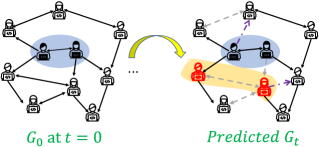
Figure 1. An example of RT$l$R query.

Note: the given users’ group $\mathcal{U}$ are marked as black icons and covered by blue color, $G_{0}$ is the snapshot of the directed evolving graph $\mathcal{G}=\{G\}_{0}^{t-1}$ at time 0, and $G_{t}$ is the predicted graph snapshot of $\mathcal{G}$ at time $t$; the greyish dotted edges in $G_{t}$ represent the relationship between users exists in $\mathcal{G}$ while disappearing in $G_{t}$; the purple dotted lines represent the new adding edges in $G_{t}$; the edge of two red icons which covered by yellow color is the query result of RT$l$R problem.

Example 1.0 (Motivation).

LinkedIn is a business and employment oriented online social network. It provides a social network platform to allow members to create their profiles and ”connect” to each other, representing real-world professional relationships. Members can also post their activity information (e.g., employment Ads) on LinkedIn. The study of RT$l$R can significantly enhance the stickiness of members in LinkedIn without any budgets paid by members or LinkedIn itself.

Figure 1 presents an evolving social network with ten members and their relationships. Suppose a research group (e.g., black icons) will host an online virtual academic seminar next month. They post the seminar information on LinkedIn because they wish to attract as many researchers as possible to join their seminar in the month ahead (e.g., $G_{t}$). By answering the RT$l$R query, LinkedIn can find out the optimal estranged relationships (e.g., among the greyish dotted edges), in which reconnecting them (e.g., red icons) will maximize the spread of seminar information in the coming month. To reconnect the estranged relationships, a possible way is to send an email to the related users’ platform Inbox and notify them of the recent news of their old friends. Therefore, the study of RT$l$R query will benefit both users and the social media platform. The members will be more willing to keep active in the network platforms, which provide them a free and efficient information post service.

To the best of our knowledge, this is the first IM study that draws the inspiration from the intersection of (1) topology evolving prediction of social networks, and (2) no additional cost. As a result, the following challenges are important to be addressed.

Challenges. The first challenge is how to predict the topology of social networks in a specified future period. To deal with this challenge, we adopt the link prediction method (Zhang et al., 2021b) to predict the network structure evolution in evolving networks. The other challenge is the complexity of RT$l$R query problem. Unlike traditional IM studies that aim to find Top-$k$ influential users, our RT$l$R focuses on the edges discovery. The existing IM algorithms are not applicable to address the RT$l$R query, and a more detailed analysis is presented in Section 4.1. Thirdly, our RT$l$R query may return different results for different given user groups, while the IM problem only needs to be queried one time to get the most influential users.

To address these algorithmic challenges, we first propose a sketched-based greedy (SBG) algorithm to answer the RT$l$R query of a given group. Besides, a candidate edges reducing method has been proposed to boost the SBG algorithm’s efficiency. Furthermore, we carefully designed a novel order-based SBG algorithm to accelerate the RT$l$R query.

Contributions. We state our major contributions as follows:

• We introduce and formally define the problem of Reconnecting Top-$l$ Relationships (RT$l$R) for the first time, and explain the motivation of solving the problem with real applications. We also prove that the RT$l$R query problem is NP-hard.

• We propose a sketch-based greedy (SBG) approach to answer the RT$l$R queries. Besides, we present the pruning method to boost the efficiency of the SBG algorithm by reducing the number of candidate edges’ probing.

• To further accelerate the RT$l$R query, we elaborately design a novel order-based algorithm to answer the RT$l$R query more efficiently.

• We conduct extensive experiments to demonstrate the efficiency and effectiveness of our proposed algorithms using real-world datasets.

Organization. The remainder of this paper is organized as follows. First, we present the preliminaries in Section 2 and formally define the RT$l$R problem in Section 3. Then, we propose the sketch-based greedy approach and the accelerate method in Section 4. We further present a new order-based algorithm to efficiently answer the RT$l$R query in Section 5. After that, the experimental evaluation and results are reported in Section 6. Finally, we review the related works in Section 7 and conclude this work in Section 8.

2. Preliminary

Table 1. Frequently used notations

Notation	Definition and Description
$\mathcal{G}=\{G\}^{t-1}_{0}$	a directed evolving graph
$G_{i}$	the snapshot graph of $\mathcal{G}$ at time point $i$
$V$; $E_{i}$	the vertex set and edge set of $G_{i}$
$G_{t}$	the predict snapshot graph of $\mathcal{G}$ at time point $t$
$\mathcal{U}$	the given users group
$I(\mathcal{U},G)$	the number of activated users in graph $G$ by users in $\mathcal{U}$
$E(I(\mathcal{U},G))$	the expected number of users in graph $G$ that influenced by users set $\mathcal{U}$
$\theta_{1}$	the number of generated RR sets
$S$ ($S_{e}$)	Candidate seed users (edges) set of IM (RT$l$R) query problem
$G_{t}\oplus S_{e}$	Reconnecting the edges in $S_{e}$ of graph $G_{t}$
$OPT$ ($OPT^{*}$)	the maximum expected spread of any size-$k$ seed users (edges) set of IM (RT$l$R) query problem
$\theta_{2}$	the number of generated sketch subgraphs
$G_{sg}=\{G^{j}_{sg}\}^{\theta_{2}}_{1}$	the sketch subgraph set
$\theta_{3}$	the number of generated sketch subgraphs in the SBG method

We define a directed evolving network as a sequence of graph snapshots $\mathcal{G}=\{G_{i}\}_{0}^{t-1}$, and $\{0,,1,..,t-1\}$ is a set of time points. We assume that the network snapshots in $\mathcal{G}$ share the same vertex set. Let $G_{i}$ represent the network snapshot at timestamp $i\in[0,t-1]$, where each vertex $u$ in $V$ is a social user in $G_{i}$, each edge $e=(u,v)$ in $E_{i}$ represents a cyber link or a social relationship between users $u$ and $v$ in $G_{i}$. Similar to (Jia et al., 2021; Das et al., 2019), we can create “dummy” vertices at each time step $i$ to represent the case of vertices joining or leaving the network at time $i$ (e.g., $V=\cup_{i=1}^{t-1}V^{i}$ where $V^{i}$ is the set of vertices truly exist at $i$). Besides, each edge $(u,v)\in E$ in $G$ is associated with a propagation probability $p(u,v)\in[0,1]$. Table 1 summarizes the mathematical notations frequently used throughout this paper.

2.1. Link Prediction

Link prediction is an important network-related problem firstly proposed by Liben-Nowell et al. (Liben-Nowell and Kleinberg, 2003), which aims to infer the existence of new links or still unknown interactions between pairs of nodes based on their properties and the currently observed links.

Given a directed evolving graph $\mathcal{G}={G_{i}}^{t-1}_{0}$ with the time points set $\{0,1,..,t-1\}$, in this paper, we use the recent link prediction method (Zhang and Chen, 2018; Zhang et al., 2021b), named learning from Subgraphs, Embeddings, and Attributes for Link prediction (SEAL) method, to predict the graph structure of snapshot graph $G_{t}$ of $\mathcal{G}$ at the future time point $t$. Specifically, SEAL is a graph neural network (GNN) based link prediction method that transforms the traditional link prediction problem into the subgraph classification problem. It first extracts the $h$-hop enclosing subgraph for each target link, and then applies a labeling trick, called Double Radius Node Labeling (DRNL), to add an integer label for each node relevant to the target link as its additional feature. Next, the above-labeled enclosing subgraphs are fed to GNN to classify the existence of links. Finally, it returns the predicted graph $G_{t}$ of evolving graph $\mathcal{G}$ at time point $t$.

2.2. Influence Maximization (IM) Problem

To better understand the IM problem, we first introduce the influence diffusion evaluation of given users.

The independent cascade (IC) model (Kempe et al., 2003) is the widely adopted stochastic model which is used for modeling the influence propagation in social networks. In the IC model, for each graph snapshot $G_{i}$, the propagation probability $p(u,v)$ of an edge $(u,v)$ is used to measure the social impact from user $u$ to $v$. This probability is generally set as $p(u,v)=\frac{1}{d(v)}$, where $d(v)$ is the degree of $v$. Every user is either in an activated state or inactive state. $S_{0}$ be a set of initial activated users, and generates the active set $S_{t}$ for all time step $t\geq 1$ according to the following randomized rule. At every time step $t\geq 1$, we first set $S_{t}$ to be $S_{t-1}$; Each user $u$ activated in time step $t$ has one chance to activate his or her neighbours $v$ with success probability $p(u,v)$. If successful, we then add $v$ into $S_{t}$ and change the status of $v$ to activated. This process continues until no more possible user activation. Finally, $S_{t}$ is returned as the activated user set of $S_{0}$.

Let $I(S,G_{i})$ be the number of vertices that are activated by $S$ in graph snapshot $G_{i}$ on the above influence propagation process under the IC model. The IM problem aims to find a size-$k$ seed set $S$ with the maximum expected spread $E(I(S,G_{i}))$. We define the IM problem as follows:

Definition 2.0 (IM problem (Kempe et al., 2003)).

Given a directed graph snapshot $G_{i}=(V,E_{i})$, an integer $k$, the IM problem aims to find an optimal seed set $S^{*}$ satisfying,

(1) $$S^{*}=\mathop{\arg\max}_{S\subseteq V,|S|=k}E(I(S,G_{i}))$$

Let $OPT$ be the maximum expected spread of any size-$k$ seed set, then we have $OPT=E(I(S^{*},G_{i}))$.

2.3. Reverse Reachable Sketch

The Reverse Influence Set (RIS) (Borgs et al., 2014) sampling technique is a Reverse Reachable Sketch-based method to solve the IM problem. By reversing the influence diffusion direction and conducting reverse Monte Carlo sampling (Kroese et al., 2014), RIS can significantly improve the theoretical run time bound.

Definition 2.0 (Reverse Reachable Set (Borgs et al., 2014)).

Suppose a user $v$ is randomly selected from $V$. The reverse reachable (RR) set of $v$ is generated by first sampling a graph $g$ from $G_{i}$, and then taking the set of users that can reach to $v$ in $g$.

By generating $\theta_{1}$ RR sets on random users, we can transform the IM problem to find the optimal seed set $S$, while $S$ can cover most RR sets. This is because if a user has a significant influence on other users, this user will have a higher probability of appearing in the RR sets. Besides, Tang et al. (Tang et al., 2014b) proved that when $\theta_{1}$ is sufficiently large, RIS returns near-optimal results with at least $1-|V|^{-1}$ probability. Therefore, the process of using the RIS method to solve the IM query contains the following steps:

• Generate $\theta_{1}$ random RR sets from $G_{i}$.

• Find the optimal user set $S$ which can cover the maximum number of above generated RR sets.

• Return the user set $S$ as the query result of IM query problem.

Theorem 2.3 (Complexity of RIS (Tang et al., 2014a)).

If $\theta_{1}\geq(8+2\varepsilon)\cdot|V|\cdot\dfrac{ln|V|+ln{|V|\choose k}+ln2}{OPT\cdot e^{2}}$, RIS returns an $(1-\frac{1}{e}-\varepsilon)$ approximate solution to the IM problem with at least $1-|V|^{-1}$ probability.

2.4. Forward Influence Sketch

The Forward Influence Sketch (FI-SKETCH) method (Cohen et al., 2014; Cheng et al., 2013; Ohsaka et al., 2014) constructs a sketch by extracting the subgraph induced by an instance of the influence process (e.g., the IC model). Then, it can estimate the influence spread of a seed set $S$ using these subgraphs accurately with theoretical guarantee. The process of using the FI-SKETCH method to solve the IM query contains the following steps:

• Generate $\theta_{2}$ sketch subgraph $G^{j}_{sg}$ by removing each edge $e=(u,v)$ from $G_{i}$ with probability $1-P_{u,v}$.

• Find the optimal user set $S$, while the average number of users reached by $S$ within $\theta_{2}$ constructed sketches graphs is maximum.

• Return the user set $S$ as the query result of IM query problem.

Theorem 2.4 (Complexity of FI-SKETCH (Cheng et al., 2013)).

If $\theta_{2}\geq(8+2\varepsilon)\cdot|V|\cdot\dfrac{ln|V|+ln{|V|\choose k}+ln2}{\varepsilon^{2}}$, FI-SKETCH returns an $(1-\frac{1}{e}-\varepsilon)$ approximate solution to the IM problem with at least $1-|V|^{-1}$ probability.

3. Problem Definition

In this section, we formulate the Reconnecting Top-$l$ Relationships (RT$l$R) query problem and analyze its complexity.

Definition 3.0 (RT$l$R Problem).

Given a directed evolving graph $\mathcal{G}=\{G_{i}\}^{t-1}_{0}$, the parameter $l$, and a group of users $\mathcal{U}$, the problem of Reconnecting Top-$l$ Relationships (RT$l$R) asks for finding an optimal edge set $S$ with size $l$ in predicted graph snapshot $G_{t}$ of $\mathcal{G}$ at time $t$, where the expected spread of $\mathcal{U}$ will be maximized while reconnecting edges of $S_{e}$ in $G_{t}$ (e.g., $\widehat{G_{t}}=G_{t}\oplus S_{e}$). Formally,

(2) $$\widehat{S_{e}}=\mathop{\arg\max}_{S_{e}\subseteq\mathcal{G}\setminus G_{t}}E(I(\mathcal{U},\widehat{G_{t}})\\ \\$$

In the following, we conduct a theoretical analysis on the hardness of the RT$l$R problem.

Theorem 3.2 (Complexity).

The RT$l$R problem is NP-hard.

Proof.

We prove the hardness of RT$l$R problem by a reduction from the decision version of the maximum coverage (MC) problem (Karp, 1972). Given an integer $l$ and several sets where the sets may have some elements in common, the maximum coverage problem aims to select at most $l$ of these sets to cover the maximum number of elements. Furthermore, we need to discuss the existence of a solution that the MC problem is reducible to the RT$l$L problem in polynomial time.

Given a directed evolving graph $\mathcal{G}$, a group of users $\mathcal{U}$, and the predicted snapshot graph $G_{t}$ from $\mathcal{G}$, we reduce the MC problem to RT$l$L with the following process: (1) For a given group $\mathcal{U}$, we compute the influence users set of $\mathcal{U}$ as $I(\mathcal{U},G_{t})$; (2) $\forall e\in\mathcal{G}\setminus G_{t}$, we create a set $S_{e}$ with the elements collected from the influenced users $I(\mathcal{U},\widehat{G_{t}})-I(\mathcal{U},G_{t})$ while $\widehat{G_{t}}=G_{t}\oplus e$; (3) We set the reconnecting edges of RT$l$L as $l$, which is the same as the input of $MC$. The above reduction can be done in polynomial time. Since the Maximum Coverage problem is NP-hard, so is the RT$l$L problem. ∎

Theorem 3.3 (Influence Spread).

The influence spread function $I(.)$ under the RT$l$R problem is monotone and submodular.

Proof.

Given a snapshot graph $G_{t}$, and a group $\mathcal{U}\in V(G_{t})$, $I(\mathcal{U},G_{t})$ represents the influenced user set of $\mathcal{U}$. For two edge sets $S_{e}\subseteq T_{e}$, we have $I(\mathcal{U},G_{t}\oplus S_{e})\leq I(\mathcal{U},G_{t}\oplus T_{e})$. Then, we have verified that $I(.)$ is monotone. Besides, for a new reconnecting edge $e$, the marginal contribution when added to set $S_{e}$ and $T_{e}$ respectively satisfies $I(\mathcal{U},G_{t}\oplus(S_{e}\cup e))-I(\mathcal{U},G_{t}\oplus S_{e})\geq I(\mathcal{U},G_{t}\oplus(T_{e}\cup e))-I(\mathcal{U},G_{t}\oplus T_{e})$. Therefore, we have proved that $I(.)$ is submodular. Thus, we can conclude that the influence spread function $I(.)$ of RT$l$L problem is monotone and submodular. ∎

4. Sketch based Greedy Algorithm

To answer the RT$l$R query problem, we first predict the graph structure of the given evolving graph $\mathcal{G}$ at $t$ by using the link prediction method (Zhang et al., 2021b). According to Theorem 3.3, the influence spread function of RT$l$R is submodularity and monotonicity. Therefore, one possible solution of the RT$l$L problem is to use the greedy approach to iteratively find out the most influential edge $e$, in which reconnecting $e$ in predicted snapshot graph $G_{t}$ will maximize the influence spread of given users group $\mathcal{U}$ in $\widehat{G_{t}}$ (e.g., $\widehat{G_{t}}=G_{t}\oplus e$). So far, the remaining challenge of RT$l$R query is to evaluate the effect of a reconnected edge $e$ on the influence spread of $\mathcal{U}$ in $G_{t}$.

4.1. Existing IM Approaches Analysis

As mentioned in (Kempe et al., 2003), we can estimate the influence spread of given users by using the Monte Carlo simulation. Specifically, given users group $\mathcal{U}$, we simulate the randomized diffusion process with $\mathcal{U}$ in $G_{t}$ for $\mathcal{R}$ times. Each time we count the number of active users after the diffusion ends, and then we take the average of these counts over the $\mathcal{R}$ times as the estimated number of influenced users of $\mathcal{U}$. However, the Monte Carlo simulation method is much time-consuming and cannot be used in the large graph. Later on, Borgs et al. (Borgs et al., 2014) proposed a Reverse Reachable Sketch-based method to the IM problem, named Reverse Influence Set (RIS) sampling, and the extended versions of the RIS method (Tang et al., 2014a; Nguyen et al., 2016, 2017) were widely used to answer the IM problem as the state-of-the-art IM query methods. The Reverse Influence Set (RIS) sampling technique is a Reverse Reachable Sketch-based method to the IM problem. By reversing the influence diffusion direction and conducting reverse Monte Carlo sampling, RIS can significantly improve the theoretical run time bound of the IM problem.

Unfortunately, the RIS sampling method is not suitable for answering our RT$l$R query. That is because the RIS sampling is designed to find the Top-$k$ most influential users in a graph, but our RT$l$R query focuses on reconnecting several optimal edges to enhance a given user group’s influence spread. In particular, the RIS sampling method transforms the IM problem to find the optimal seed set $S$ by generating $\theta_{1}$ RR sets, while $S$ can cover most RR sets. The RR sets only contain the user’s information while discarding the graph sketch (e.g., the edge’s information). Therefore, if we use the RIS sampling to answer the RT$l$R query, we have to recompute the RR sets for each edge insertion during the RT$l$R query process, which is time-consuming and unrealistic in large graphs.

4.2. FI-Sketch based Greedy Algorithm

Facing the challenges mentioned above, we propose a sketch-based greedy (SBG) method to answer the RT$l$R query. Precisely, we first set $\theta_{3}$ as a sufficient number of generated sketch subgraphs in our SBG method to theoretically ensure the quality of the returned results for the RT$l$R query (i.e., the details of how $\theta_{3}$ should be set will further discuss in Section 4.3). Then, we use the FI-SKETCH to evaluate the effect of a new adding edge $e$ on the influence spread of a given users group $\mathcal{U}$ based on the $\theta_{3}$ generated sketch subgraphs. Compared with the RIS approach, the graph structure information was contained in the generated $\theta_{3}$ sketch subgraphs during the process of the FI-SKETCH approach (refer to Section 2.4), so that we do not need to recompute the sketches while the edges update.

Input: $\mathcal{G}=\{G_{i}\}^{t-1}_{0}:$ an evolving graph, $l$: the number of selected edges, and $\mathcal{U}$: a group of users

Output: $\widehat{S_{e}}:$ the optimal reconnecting edge set

1 Predict the snapshot graph $G_{t}$ from $\mathcal{G}$ (Zhang et al., 2021b);

2 Generate $\theta_{3}$ sketch subgraph $G_{sg}=\{G^{j}_{sg}\}_{1}^{\theta_{3}}$;

3 Initialize $\widehat{S_{e}}\leftarrow\emptyset$, Candidate edges set $CE\in\{\mathcal{G}\setminus G_{t}\}$;

4 for $i=1$ to $l$ do

5       $\widehat{e}\leftarrow\mathop{\arg\max}_{e\in CE}$ FI-SKETCH$(\mathcal{U},e)$;

6       $\widehat{S_{e}}\leftarrow\widehat{S_{e}}\cup\widehat{e}$;

7      

8return $\widehat{S_{e}}$

9 Function FI-SKETCH($\mathcal{U},e$):

10       $count\leftarrow 0$;

11       for $j=1$ to $\theta_{3}$ do

12             $\widehat{G^{j}_{sg}}\leftarrow G^{j}_{sg}\oplus\{\widehat{S_{e}}\cup e\}$;

13             $n_{a}\leftarrow$ the number of vertexes reached by $\mathcal{U}$ in $\widehat{G^{j}_{sg}}$;

14             $count\leftarrow count+n_{a}$;

15            

16      return $\dfrac{count}{\theta_{3}}$

End Function

Algorithm 1 RT$l$R: SBG

The details of the SBG method are described in Algorithm 1. In the pre-computing phase (Lines 1-1), we predict the snapshot graph $G_{t}$ using the link prediction method (Zhang et al., 2021b), and then generate $\theta_{3}$ random sketch graphs by removing each edge $e=(u,v)$ from $G_{t}$ with probability $1-P_{u,v}$. Besides, based on Definition 3.1, we initialize $CE\in\{\mathcal{G}\setminus G_{t}\}$ as the candidate edges set of the RT$l$R query. In the main body of SBG (Lines 1-1), we use the greedy method to iteratively find the $l$ number of optimal reconnecting edges. Specifically, in each iterative, we call the FI-SKETCH Function to find out the optimal edge $\widehat{e}$ from the candidate edge set $CE$ and add $\widehat{e}$ into set $\widehat{S_{e}}$ , while reconnecting the selected edge can maximize the influence diffusion of given users group $\mathcal{U}$. Meanwhile, given an edge $e$, the FI-SKETCH Function returns back the influenced users evaluation results by using the Forward Influence Sketch method mentioned in Section 2.4 (Lines 1-1). Finally, we return edges set $\widehat{S_{e}}$ as the result of RT$l$R query (Line 1).

Complexity. The time complexity of calling the FI-SKETCH function for each candidate edges is $\mathcal{O}(\theta_{3}\cdot|E_{t}|)$, while the space complexity is $\mathcal{O}(\theta_{3}\cdot(|V|+|E_{t}|))$. Hence, the time complexity and space complexity of SBG algorithm are $\mathcal{O}(l\cdot|CE|\cdot\theta_{3}\cdot|E_{t}|$) and $\mathcal{O}(\theta_{3}\cdot(|V|+|E_{t}|))$, respectively.

4.3. Theoretical Analysis of SBG

In this part, we will establish our theoretical claims for SBG. Specifically, we analyze how $\theta_{3}$ should be set to ensure our SBG method returns near-optimal results to RT$l$R query with high probability. Our analysis highly relies on the Chernoff bounds (Hoeffding, 1963).

Lemma 4.0.

Let $X_{1}$,…,$X_{r}$ be $r$ number of independent random variables in $[0,1]$ and $X=$ with a mean $\mu$. For any $\sigma>0$, we have

(3) $$\begin{split}&Pr[X-r\mu\geq\sigma\cdot r\mu]\leq exp(-\frac{\sigma^{2}}{2+\sigma}r\mu),\\ &Pr[X-r\mu\leq-\sigma\cdot r\mu]\leq exp(-\frac{\sigma^{2}}{2}r\mu).\end{split}$$

Let $\mathcal{U}$ be a group of users, $S_{e}$ be the selected reconnecting edges, $\mathcal{R}_{2}$ be the number of generated sketch subgraphs in the SBG algorithm (Algorithm 1), and $F_{R}(\mathcal{U},S_{e})$ be the total number of additional reached users by $\mathcal{U}$ in each sketch subgraph after reconnecting edges in $S_{e}$. From (Ohsaka et al., 2014), the expected value of $\frac{F_{R}(\mathcal{U},S_{e})}{\mathcal{R}_{2}}$ equals the expected influence diffusion enhance by reconnecting edges of $S_{e}$ in $G_{t}$. Then, we have the following lemma.

Lemma 4.0.

$E[\frac{F_{R}(\mathcal{U},S_{e})}{\mathcal{R}_{2}}]=E[I(\mathcal{U},G_{t}\oplus S_{e})-I(\mathcal{U},G_{t})]$

Proof.

Each sketch subgraph in the SBG algorithm is generated by removing each edge $e$ with $1-p(e)$ probability. From (Ohsaka et al., 2014), we can observe that the expected value of the average number of reached users to $\mathcal{U}$ in all sketch subgraphs is equal to the expected spread of $\mathcal{U}$ in $G_{t}$. From the above relation of equality, we can easily deduce that $E[\frac{F_{R}(\mathcal{U},S_{e})}{\mathcal{R}_{2}}]=E[I(\mathcal{U},G_{t}\oplus S_{e})-I(\mathcal{U},G_{t})]$. ∎

Theorem 4.3 (Approximate ratio).

By generating $\theta_{3}$ sketch subgraphs with $\theta_{3}\geq(8+2\varepsilon)\cdot|V|\cdot\dfrac{ln|V|+ln{|V|\choose l}+ln2}{\varepsilon^{2}}$, we have $|\frac{F(\mathcal{U},S_{e})}{\theta_{3}}-(E[I(\mathcal{U},G_{t}\oplus S_{e})-I(\mathcal{U},G_{t})])|<\frac{\varepsilon}{2}$ holds with probability $1-|V|^{-l}$ simultaneously for all selected edges set $S$ (i.e., $|S|=l$).

Proof.

We can prove Theorem 4.3 by tweaking the proof in Theorem 2.3 of (Tang et al., 2014a). Let $\rho$ be the probability of $\mathcal{U}$ can activate a fixed user $v$ after reconnecting edges in $S_{e}$ in $G_{t}$. Based on Lemma 4.2,

(4) $$\rho=E[\frac{F_{R}(\mathcal{U},S_{e})}{\mathcal{R}_{2}}]/|V|=(E[I(\mathcal{U},G_{t}\oplus S_{e})-I(\mathcal{U},G_{t})])/|V|$$

Then, we have

(5) $$\begin{split}Pr&[|\frac{F_{R}(\mathcal{U},S_{e})}{\theta_{3}}-(E[I(\mathcal{U},G_{t}\oplus S_{e})-I(\mathcal{U},G_{t})])|]\geq\frac{\varepsilon}{2}\\ &=Pr[|\frac{F_{R}(\mathcal{U},S_{e})}{|V|}-\rho\theta_{3}|]\geq\frac{\varepsilon\theta_{3}}{2|V|}\end{split}$$

Let $\sigma=\frac{\varepsilon}{2|V|\rho}$. Based on Lemma 4.1, we have

(6) $$\begin{split}Equation~{}(\ref{eq:prop})<&2\cdot exp(-\frac{\sigma^{2}}{2+\sigma}\cdot\rho\cdot\theta_{3})\\ &=2\cdot exp(\frac{\varepsilon^{2}}{8|V|^{2}\rho+2|V|\varepsilon}\cdot\theta_{3})\\ &\leq 2\cdot exp(-\frac{\varepsilon^{2}}{8|V|+2\varepsilon|V|}\cdot\theta_{3})\\ &\leq\frac{1}{|V|^{l}}.\end{split}$$

Thus, Theorem 4.3 is proved. ∎

Theorem 4.4 (Complexity of SBG).

With a probability of $1-|V|^{-l}$, the SBG method for solving the RT$l$R query problem requires $\theta_{3}\geq(8+2\varepsilon)\cdot|V|\cdot\dfrac{ln|V|+ln{|V|\choose k}+ln2}{\varepsilon^{2}}$ number of sampling sketch subgraphs so that an $(1-\frac{1}{e}-\varepsilon)$ approximation ration is achieved.

Proof.

The proof of Theorem 4.4 is summarized as following three steps. Firstly, based on the property in Theorem 4.3, if the number of generated sampling sketch subgraphs $\theta_{3}\geq(8+2\varepsilon)\cdot|V|\cdot\dfrac{ln|V|+ln{|V|\choose k}+ln2}{\varepsilon^{2}}$, then we have $|\frac{F(\mathcal{U},S_{e})}{\theta_{3}}-(E[I(\mathcal{U},G_{t}\oplus S_{e})-I(\mathcal{U},G_{t})])|<\frac{\varepsilon}{2}$ holds with probability $1-|V|^{-l}$. Secondly, the SBG method we proposed in this paper to solve the RT$l$R problem by utilizing the greedy algorithm of maximum coverage problem (Karp, 1972), which produces a $(1-\frac{1}{e})$ approximation solution (mentioned in Theorem 3.2). Finally, by combining the above two approximation ration $\frac{\varepsilon}{2}$ and $(1-\frac{1}{e})$, we can conclude the final approximation ration of our SBG method for solving RT$l$R query problem is $(1-\frac{1}{e}-\varepsilon)$ with at least $1-|V|^{-l}$ probability. ∎

4.4. Reducing # Candidate Edges

Since the SBG algorithm’s time complexity is cost-prohibitive, which would hardly be used for dealing with the sizeable evolving graph. In this subsection, we present our optimization method by pruning the unnecessary potential edges in candidate edge set $CE$. The core idea behind this optimization strategy is to eliminate the edges in $CE$ which will not have any benefit to expend the influence spread of given users group $\mathcal{U}$ while reconnecting it.

We use the symbol $u\leftsquigarrow\mathcal{U}$ to denote that $u$ can be reached by $\mathcal{U}$. In order to reduce the size of $CE$, we present the below theorem to identify the quality reconnecting edge candidates (denote as $\widehat{CE}$) from $CE$.

Theorem 4.5 (Reachability).

Given a directed snapshot graph $G_{t}$ and a users group $\mathcal{U}$, if an edge $e=(u,v)$ is selected to reconnect, one of its related users (i.e., $u$ or $v$) requires to be reached by $\mathcal{U}$ in $G_{t}$; that is $e\in\widehat{CE}$ implies $u\leftsquigarrow\mathcal{U}$ or $v\leftsquigarrow\mathcal{U}$ in $G_{t}$.

Proof.

We prove the correctness of this theorem by contradiction. The intuition is that at least one pathway exists from a user to all of its influenced users in social networks. For the selected edge $e=(u,v)$, if both the user $u$ and $v$ are not reached by the users group $\mathcal{U}$, then the pathway between $\mathcal{U}$ and $e$ does not exist. Therefore, reconnecting the edge $e$ does not bring any benefits to the expansion of influence spread starting from $\mathcal{U}$, which contradicts with Definition 3.1. Thus, the theorem is proved. ∎

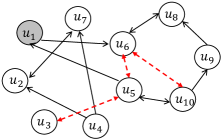
Figure 2. Running Example

Example 4.0.

Figure 2 shows a snapshot graph $G_{t}$ with $10$ nodes and $9$ edges. The candidate edges set of RT$l$R is $CE=\{(u_{3},u_{4}),(u_{5},u_{6}),\\ (u_{6},u_{10})\}$. For a given user group $\mathcal{U}=\{u_{1}\}$, the pruned candidate edge set would be $\widehat{CE}=\{(u_{5},u_{6}),(u_{6},u_{10})\}$ due to $u_{6}\leftsquigarrow\mathcal{U}$.

Based on Theorem 4.5, we present a BFS-based method for pruning the candidate edge set $CE$ in graph $G_{t}$ with a given users group $\mathcal{U}$. The core idea of the BFS-based algorithm is to traverse the graph $G_{t}$ starting from the nodes in $\mathcal{U}$ by performing breadth-first search (BFS). For edges in $CE$, if both of its related nodes are not visited in the above BFS process, then we directly prune it.

In Algorithm 2, we outline the major steps of the BFS-based method for processing the $CE$ pruning. Initially, each user $u$ in graph $G_{t}$ are marked a visiting status as FALSE (Line 2). Then, for the users in a given group $\mathcal{U}$, we update its visiting status as TRUE (Lines 2-2). Further, we process a BFS search starting from root user $v\in\mathcal{U}$, and update the status of each visited users as TRUE (Lines 2-2). Next, based on Theorem 4.5, we reduce all candidate edges $e=(u,v)$ from $CE$ while both $u$ and $v$ have the FALSE visited status (Lines 2-2), and finally, we return the pruned candidate edges set $\widehat{CE}$ (Line 2).

1 Initialize set $\widehat{CE}\leftarrow\emptyset$, an empty Queue $Q$;

2 Initialize visited array $A$ with size $|V|$ as FALSE;

3

4for each $u\in U$ do

5       $A[u]=TRUE$;

6       Enqueue $u$ into $Q$;

7      

8while $Q$ is not empty do

9       Dequeue $v$ from $Q$;

10       for each neighbor $v^{\prime}\in nbr(v,G_{t})$ in $G_{t}$ do

11             if $A[v^{\prime}]=FALSE$ then

12                   $A[v^{\prime}]=TRUE$, Enqueue $v^{\prime}$ into $Q$;

13                  

14            else

15                   Continue;

16                  

17            

18      

19for $e=(u,v)\in CE$ do

20       if $A[u]=TRUE$ or $A[v]=TRUE$ then

21             add $e$ into $\widehat{CE}$

22      else

23             continue;

24      

return $\widehat{CE}$

Algorithm 2 Reducing $CE$ $\#$ BFS $(CE,\mathcal{U})$

Complexity. Obviously, for a given group $\mathcal{U}$, the time complexity of Algorithm 2 is $\mathcal{O}(|V|+|E_{t}|+|CE|)$, and the space complexity is $\mathcal{O}(|V|)$. Furthermore, the occupied space by Algorithm 2 will be released after the pruned candidate edges $\widehat{CE}$ is returned. For each RT$l$R query with a new given users group $\mathcal{U}$ as input, we need to recall the BFS-based pruning method to reduce the size of candidate set $CE$ with time cost $\mathcal{O}(|V|+|E_{t}|+|CE|)$, which is the main drawback of the BFS-based pruning method.

5. The Improvement Algorithm

Although the SBG algorithm and its optimization method can successfully answer the RT$l$R query problem, it is still time-consuming to handle the sizeable social networks. To address this limitation, in this section, we propose an ordered sketch-based greedy algorithm, which can significantly reduce the number of edges influence probing at each iterative of RT$l$R query process, so as to answer the RT$l$R query more efficiently.

5.1. Algorithm Overview

Let $\mathcal{G}=\{G_{0},G_{1},...,G_{t-1}\}$ be an evolving graph. We first use the temporal link prediction method (Zhu et al., 2016) to predict the future snapshot of graph $G_{t}$, and the potential reconnecting edges will be selected from candidate edges set $CE=\{\mathcal{G}\setminus G_{t}\}$. Before introducing the core idea of our Order-based SBG algorithm, we first briefly review using the SBG algorithm to answer the RT$l$R query and analyze the bottleneck of the SBG algorithm.

For each given users group $\mathcal{U}$, the SBG algorithm aims to find $l$ reconnecting edges by iteratively probing each edge in $CE$ to find out the edge $\widehat{e}$ in which reconnecting $\widehat{e}$ will bring the maximum benefits to the influence spread of $\mathcal{U}$. The time complexity of influence spread by reconnection of an edge is $\mathcal{O}(\theta_{3}\cdot|E_{t}|)$, which is the bottleneck of the SBG algorithm.

To deal with the above limitation of the SBG method, we propose an Order-based SBG algorithm, which focuses on reducing the number of edges probing in each iteration by using our elaboratively designed two-step bounds approach together with the order-based probing strategy. Specifically, we first generate a label index (UBL) to store the first step upper bound of influence spread expansion for each candidate edge $e\in CE$ w.r.t $UB_{1}(e)$ (in Section 5.2). Then, we generate the initial second-step upper bound ($UB_{2}$) for $e$ (i.e., $UB_{2}.e$) from $UB_{1}(e)$ of the UBL index. Next, in the influence spread expansion estimation query processing of each given users group $\mathcal{U}$ and probing edge $e$, we narrow the second-step upper bound of $e$ and update the $UB_{1}(e)$ value of UBL index, while the narrowed second-step upper bound will be served the optimal edge finding in the following iterations (in Section 5.3). Finally, we order the candidate edges by their $UB_{2}$ values. The edge probing at the current iteration will be early terminated while the second upper bound of probing edge $e$ is less than the present influence spread expansion estimation value (in Section 5.4).

5.2. Upper Bound Label (UBL) Construction

This section introduces how to build the label index (UBL) for each candidate edge. The UBL index contains two parts, including (1) the $\theta_{3}$ sketch subgraphs $G_{sg}$; (2) the first-step bound $UB_{1}(e)$ of each candidate edge $e$ and its updating status. The details of UBL construction procedure is shown in Algorithm 3.

1 ($\mathcal{L}$, $G_{sg}$) $\leftarrow(\emptyset,\emptyset)$;

2 Generate $\theta_{3}$ sketch subgraph $G_{sg}=\{G^{j}_{sg}\}_{1}^{\theta_{3}}$;

3 for each edge $e=(u,v)\in CE$ do

4       $UB_{1}(e)\leftarrow$ the number of vertices that can be reached from $v$ in $G_{t}$;

5       $flag(e)\leftarrow 0$;

6       add $(UB_{1}(e),flag(e))$ into $\mathcal{L}$;

7      

Store ($\mathcal{L}$, $G_{sg}$)

Algorithm 3 Build UBL($\mathcal{L}$, $G_{sg}$)

From Section 2.4, we first generate $\theta_{3}$ sketch subgraphs from the predicted snapshot graph $G_{t}$ that will be used for the future influence spread estimation (Line 3). Then, for each candidate edge $e$ in $CE$, we initialize its updating mark (i.e., $flag(e)$) as $0$. Meanwhile, we compute the number of vertices in $G_{t}$ that can be reached from $e$ as the first step upper bound of $e$, denoted as $UB_{1}(e)$ (Lines 3 - 3). Finally, we store the Labeling Scheme ($\mathcal{L}$, $G_{sg}$) for RT$l$R query processing (Line 3).

Complexity. The time complexity of sketch subgraphs generation is $\mathcal{O}(\theta_{3}\cdot|E_{t}|)$, and the $UB_{1}$ labeling construction of all candidate edges in $CE$ is $O(|CE|\cdot|E_{t}|)$. Therefore, the time complexity of UBL construction is $\mathcal{O}(\theta_{3}\cdot|E_{t}|+|CE|\cdot|E_{t}|)$. Besides, the space complexity of UBL index construction is $\mathcal{O}(\theta_{3}\cdot(|V|+|E_{t}|)+|CE|)$, while storage sketch subgraphs $G_{sg}$ has space complexity $O(\theta_{3}\cdot(|V|+|E_{t}|))$ and generating $UB_{1}$ labeling of edges in $CE$ has space complexity of $\mathcal{O}(|CE|)$.

5.3. Influence Spread Expanding Estimation

Here, we present the influence spread expansion estimation of given users group $\mathcal{U}$ and edge $e$. Further, we also introduce the strategies of narrowing the two-step upper bounds of $e$ (i.e., $UB_{1}(e)$ and $UB_{2}(e)$) during the above estimation process.

1 Function Sketch-Estimate($\mathcal{U},e$):

2       $count\leftarrow 0$, $count_{R}\leftarrow 0$, $e=(u,v)$;

3       for $k=1$ to $\theta_{3}$ do

4             while $SG[k][u]==1$ $\&\&$ $SG[k][v]==0$ do

5                   $n_{a}\leftarrow|\{u^{\prime}\in V|u^{\prime}\leftsquigarrow e$ in $G^{k}_{sg}\ \wedge$  $SG[k][u^{\prime}]==0\}|$;

6                   $count\leftarrow count+n_{a}$;

7                  

8            if $\mathcal{L}.flag(e)==0$ then

9                   $n_{R}\leftarrow|\{u^{\prime}\in V|u^{\prime}\leftsquigarrow e$ in $G^{k}_{sg}\}|$ ;

10                   $count_{R}\leftarrow count_{R}+n_{R}$;

11                  

12            else

13                   continue;

14                  

15            

16      update $(e,UB_{2}.e)\leftarrow(e,count/\theta_{3})$ of $Q$;

17       if $\mathcal{L}.flag(e)==0$ then

18             update $(UB_{1}(e),flag(e))\leftarrow(count_{R}/R,1)$ of $\mathcal{L}$;

19             $\mathcal{L}.flag(e)\leftarrow 1$;

20            

21      return $count/\theta_{3}$

End Function

Algorithm 4 Sketch-Estimate Function

The details of the influence spread expansion estimation are described in Algorithm 4. For a given users group $\mathcal{U}$ and edge $e=(u,v)$, the Sketch-Estimate Function aims to compute the incremental of $\mathcal{U}$’s influence spread while reconnecting edge $e$ in graph $G_{t}$. It takes sketch subgraphs $G_{sg}$, query edge $e$ and group $\mathcal{U}$, influenced marking array $SG$, two-step bound $UB_{1}$ and $UB_{2}$, and returns the influence spread expansion value of $e$ to $\mathcal{U}$. We initialize two variable $count$ and $count_{R}$ as $0$ (Line 4). Then, an inner loop fetches the total number of the reached nodes $v$ for $e$ in each sketch subgraph $G^{k}_{sg}\in G_{sg}$ but not be reached by $\mathcal{U}$ (i.e., $SG[k][v]==0$), and we use $count$ to record it (Lines 4-4). Meanwhile, if the first step upper bound of $e$ is never updated (i.e., $\mathcal{L}.flag(e)==0$), we further compute the total number of nodes reached by $e$ in each sketch graph of $G_{sg}$, and store the result in $count_{R}$ (Lines 4 - 4). Next, we update the value of $UB_{2}$ as $count/\theta_{3}$, which is also the influence spread expansion value of $e$ (Line 4); we also update $UB_{1}(e)$ and remark $flag(e)=1$ of $\mathcal{L}$ when the original mark $\mathcal{L}.flag(e)=0$ (Line 4 - 4). Finally, the influence spread expansion of $e$ is returned (Line 4). It is remarkable that with the increasing number of RT$l$R queries for different given users group $\mathcal{U}$, the more edges’ first-step upper bound $UB_{1}$ will be narrowed, so as to the performance of the later RT$l$R query with new users group will increase with no additional cost.

Complexity. It is easy for us to derive that the time complexity and space complexity of Algorithm 4 are $\mathcal{O}(\theta_{3}\cdot|E_{t}|)$ and $\mathcal{O}(\theta_{3}\cdot|V|)$, respectively.

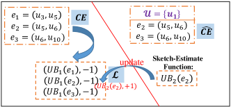
Figure 3. The Two-Step-Bounds Example

Example 5.0.

Figure 3 shows a running example of our two step bounds generation. For a given graph $G_{t}$ in Figure 2, we first identify the candidate edges set $CE=\{(u_{3},u_{5}),(u_{5},u_{6}),(u_{6},u_{10})\}$. Then, we compute the first-step bound of each edge in $CE$ (e.g., $UB_{1}(u_{3},u_{5})$) and set its initial flag as $-1$. During the process of each RT$l$L query with different given users group $\mathcal{U}$, we will prune the candidate edges set from $CE$ to $\widehat{CE}$, and call the Sketch-Estimate Function (e.g., Algorithm 4) to estimate the influence spread expansion of each probing edge (e.g., $e_{2}=(u_{5},u_{6})$) from $\widehat{CE}$. Meanwhile, during the above process, we get a byproduct of $e_{2}$, the second step upper bound $UB_{2}(e_{2})$, which can be used to narrow the first upper bound of $e_{2}$ (e.g., $UB_{1}(e_{2})\leftarrow UB_{2}(e_{2})$). Once $UB_{1}(e_{2})$ is updated, $e_{2}$’s flag also needs to be changed to $+1$.

5.4. Order-based SBG for RT$l$R Query Processing

Input: $l$: the number of selected edges, $\mathcal{U}$: users group, $CE=\mathcal{G}\setminus G_{t}$: candidate edges, and ($\mathcal{L}$, $G_{sg}$): UBL

Output: $\widehat{S}:$ the optimal Reconnecting edge set

1

2Initialize $\widehat{S}\leftarrow\emptyset$, Priority queue $Q$, and Array $SG[\theta_{3}][|V|]$;

3 $\widehat{CE}\leftarrow$ Reducing CE # BFS $($CE$,\mathcal{U})$; /*using Algorithm 2 */

4 for each edge $e=(u,v)\in\widehat{CE}$ do

5       $UB_{2}.e\leftarrow\mathcal{L}.{UB_{1}(e)}$;    push $(e,UB_{2}.e)$ into $Q$;

6      

7for $i=1$ to $\theta_{3}$ do

8       for each $u\leftsquigarrow\mathcal{U}$ in $G^{i}_{sg}$ do

9             $SG[i][u]\leftarrow 1$;

10            

11      

12

13for $j=1$ to $l$ do

14       $(e^{\prime},UB_{2}.{e^{\prime}})\leftarrow Q.front$ ;    $I_{max}\leftarrow 0$;    $\widehat{e}\leftarrow e^{\prime}$;

15       while $I_{max}<UB_{2}.{e^{\prime}}$ do

16             $I_{max}\leftarrow$ Sketch-Estimate$(\mathcal{U},e^{\prime})$;

17             $\widehat{e}\leftarrow e^{\prime}$; $(e^{\prime},UB_{2}.{e^{\prime}})\leftarrow Q.front$ ;

18            

19      $\widehat{S}\leftarrow\widehat{S}\cup\widehat{e}$;

20       for each edge $e_{ce}=(u,v)\in CE\setminus\widehat{CE}$ $\&\&$ $e_{ce}\leftsquigarrow\widehat{e}$ do

21             $\widehat{CE}\leftarrow\widehat{CE}\cup e_{ce}$; $UB_{2}.e_{ce}\leftarrow\mathcal{L}.{UB_{1}(e_{ce})}$;

22             push $(e_{ce},UB_{2}.e_{ce})$ into $Q$;

23            

24      for $m=1$ to $\theta_{3}$ do

25             $\widehat{e}=(\widehat{u},\widehat{v})$;

26             if $SG[m][\widehat{u}]==1$ $\&\&$ $SG[m][\widehat{v}]==0$ then

27                   $SG[m][\widehat{v}]\leftarrow 1$;

28                   for each $u^{\prime}\leftsquigarrow\widehat{e}$ in $G^{m}_{sg}$ do

29                         $SG[m][u^{\prime}]\leftarrow 1$;

30                        

31                  

32            else

33                   continue;

34                  

35            

36      

return $\widehat{S}$

Algorithm 5 RT$l$R: Order-based SBG

In the previous parts of this section, we have overviewed the main idea of our order-based SBG algorithm. We also have introduced the details of two essential blocks of our Order-based SBG algorithm: (i) the UBL construction and (ii) the Sketch-Estimation Function. In the rest of this section, we will discuss the details of the Order-based SBG algorithm.

The details of the Order-based SBG algorithm are described in Algorithm 5. It takes an integer $l$, a users group $\mathcal{U}$, the candidate edges $CE$, and UBL index $(\mathcal{L},G_{sg})$ as inputs, and returns a set $\widehat{S}$ of $l$ optimal reconnecting edges that maximizes the influence spread of $\mathcal{U}$. We initialize a set $\widehat{S}$ as empty, an empty Priority queue $Q$ that will be used to store the $UB_{2}$ information of candidate edges related to $\mathcal{U}$, and an array $SG$ to mark whether a node can be reached by $\mathcal{U}$ or edges in $\widehat{S}$ at each sketch subgraphs $G_{sg}$ (Line 5). Then, we reduce the candidate edges from $CE$ by using Algorithm 2, and record the reduced candidate edges into set $\widehat{CE}$ (Line 5). For each edge $e$ in $\widehat{CE}$, we get $e$’s first-step upper bound $UB_{1}(e)$ from UBL index, and set $UB_{1}(e)$ as the initial second-step upper bound value of $e$ (i.e., $UB_{2}(e)=\mathcal{L}.UB_{1}(e)$), and then push $(e,UB_{2}(e))$ into priority queue $Q$ (Lines 5 - 5). Next, we mark the nodes which are reached by $\mathcal{U}$ in each sketch subgraphs of $G_{sg}$ (Lines 5 - 5). Further, in each iteration, we probe the candidate edges in priority queue $Q$ in order based on their $UB_{2}$ value, and then call Sketch-Estimation Function to compute the influence spread expansion of the probing edge $e$, the edge probing in this iteration will be early terminated once the front edge from Q is less than the currently maximum influence spread expansion value (Line 5). After finding out the optimal edge $\widehat{e}$, we update the mark of nodes reached by $\widehat{e}$ in each sketch subgraphs (Lines 5 -5). Finally, it returns the optimal reconnecting edge set $\widehat{S}$ having maximum influence spread expansion of $\mathcal{U}$ (Line 5).

Complexity. The time complexity of Algorithm 5 is $\mathcal{O}(|\widehat{CE}|+\theta_{3}\cdot|E_{t}|+l\cdot|\widehat{CE}|\cdot\theta_{3}\cdot|E_{t}|)$. Besides, the space complexity is $\mathcal{O}(|CE|+\theta_{3}\cdot|E_{t}|)$. Although the time complexity of Algorithm 5 is not significantly better than the SBG algorithm, it can greatly reduce the number of candidate edges probing for influence spread estimation, which is the bottleneck of the SBG algorithm.

6. Experimental Evaluation

In this section, we present the experimental evaluation of our proposed approaches for the RT$l$L queries: the sketch based greedy algorithm (SBG) in Section 4.2; the candidate edges pruning method to accelerate SBG (CE-SBG) in Section 4.4; and the Order-based SBG solution (O-SBG) in Section 5.4.

6.1. Experimental Setting

We implement the algorithms using Python 3.6 on Windows environment with 2.90GHz Intel Core i7-10700 CPU and 64GB RAM.

Baseline. To the best of our knowledge, no existing work investigates the RT$l$R problem. To further validate, we use our SBG algorithm as the baseline algorithm to compare with CE-SBG and O-SBG. This is because the well-known RIS based IM methods (Tang et al., 2014a; Nguyen et al., 2016) are hardly used in the RT$l$R query (i.e., mentioned in Section 4.1). Meanwhile, our SBG algorithm is extended from the FI-sketch IM method (i.e., SG algorithm (Cohen et al., 2014)), while the SG algorithm performs well within the existing IM efforts, which has been validated in the state-of-the-art IM benchmark study (Arora et al., 2017).

Table 2. The Description of Dataset

Dataset	Nodes	Temporal Edges	$d_{avg}$	Days	Type
eu-core	986	332,334	25.28	803	Directed
CollegeMsg	1,899	59,835	10.69	193	Directed
mathoverflow	21,688	107,581	4.17	2,350	Directed
ask-ubuntu	137,517	280,102	1.91	2,613	Directed
stack-overflow	2,464,606	17,823,525	6.60	2,774	Directed

Datasets. We conduct the experiments using five publicly available datasets from the Large Network Dataset Collection : eu-core, CollegeMsg, mathoverflow, ask-ubuntu, and stack-overflow. The statistics of the datasets are shown in Table 2. We have averagely divided all datasets into $T$ graph snapshots (e.g., $G_{t}=(V,E_{t})$, $t\in[1,T]$), where $V$ is the node and $E_{t}$ is the edges appearing in the time period of $t$ in each dataset.

Parameter Configuration. Table 3 presents the parameter settings. We consider four parameters in our experiments: the number of queries $Q$, the size of given users group $|\mathcal{U}|$, reconnecting edges size $l$, and the number of snapshots $T$. Besides, the near future snapshot $G_{T+1}$ is generated by using the recent link prediction method (Zhang et al., 2021b) In each experiment, if one parameter varies, we use the default values for the other parameters. Besides, we set $\theta_{3}=200$, which is consistent with (Arora et al., 2017).

Table 3. Parameters and their values

Parameter	Values	Default
$Q$	$[20,40,60,80,100]$	80
$|\mathcal{U}|$	$[1,2,4,6,8]$	6
$l$	$[1,10,20,40]$ or $[1,2,3,4]$	10 or 2
$T$	$[20,40,60,80,100]$	100

6.2. Efficiency Evaluation

We study the efficiency of the approaches for the RT$l$L problem regarding running time under different parameter settings.

6.2.1. Varying Reconnecting Edges Set Size $l$

(a) mathoverflow

(b) ask-ubuntu

(c) CollegeMsg

(d) eu-core

Figure 4. Time cost of algorithms with varying $l$

Figure 4 shows the average running time of our proposed methods by varying $l$ between $1$ to $40$. The running time of the algorithms follows similar trends, where SBG consumes maximum time to process an RT$l$R query. On average, O-SBG is $65$ to $99$ times faster than CE-SBG, and 90 to 167 times faster than SBG. Also, CE-SBG is about $3$ to $11$ times faster than SBG in different datasets when $l$ varies from $2$ to $40$. Notably, when $l$ is larger than $30$, the SBG algorithm fails to return the result of the RT$l$R query within one day. As expected, the running time of both three approaches significantly increases when $l$ is varied from $1$ to $40$. Besides, the growth of running time in O-SBG is much slower than the other two algorithms. This is because the probing candidate edges will increase in all three approaches when $l$ increases, and O-SBG has the smallest number of probing candidate edges among the three approaches (refer to Figure 5).

(a) mathoverflow

(b) ask-ubuntu

(c) CollegeMsg

(d) eu-core

Figure 5. Number of probing edges of algorithms

The number of probing candidate edges of SBG, CE-SBG, and O-SBG with varying $l$ are presented in Figure 5(a)-5(d). As can be seen, the probing candidate edges of O-SBG is much less than SBG and CE-SBG for all values of $l$. For example, when $l=20$, the probing candidate edges of SBG, CE-SBG, and O-SBG in mathoverflow are $91,850$, $28,588$, and $547$, respectively. Besides, the number of probing candidate edges increases in all three approaches with the increase of $l$, and O-SBG probing the least number of candidate edges in all three approaches. This result has verified the above explanation about why O-SBG performs better than the other two approaches with varying $l$.

6.2.2. Varying Number of Queries $Q$

(a) mathoverflow

(b) ask-ubuntu

(c) CollegeMsg

(d) eu-core

Figure 6. Time cost of algorithms with varying $Q$

We compare the performance of different approaches by varying the number of RT$l$R queries from $20$ to $100$. Figure 6 shows the average running time of SBG, CE-SBG, and O-SBG on the four datasets. As we can see, O-SBG is significantly efficient than SBG and CE-SBG. Specifically, O-SBG performs two to three orders of magnitude faster than SBG and one to two orders of magnitude faster than CE-SBG in all datasets, respectively.

6.2.3. Varying Users Group Size $|\mathcal{U}|$

(a) mathoverflow

(b) ask-ubuntu

(c) CollegeMsg

(d) eu-core

Figure 7. Time cost of algorithms with varying $|\mathcal{U}|$

Figure 7 shows the running time of the approaches by varying the size of users group $\mathcal{U}$ from $1$ to $8$. The results show similar findings that O-SBG outperforms CE-SBG and SBG as it utilizes the two step bounds to significantly reduce the probing candidate edges. For example, O-SBG can reduce the running time by around $150$ times and $31$ times compared with SBG and CE-SBG respectively under different $|\mathcal{U}|$ settings on the mathoverflow dataset.

6.2.4. Varying Snapshot Size $T$

(a) mathoverflow

(b) ask-ubuntu

(c) CollegeMsg

(d) eu-core

Figure 8. Time cost of algorithms with varying $T$

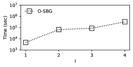
Figure 9. Performance of O-SBG on stack-overflow

We compare the efficiency of our proposed algorithms by varying the graph snapshots size $T$ from $20$ to $100$. Figure 8 presents the running time with varied values of $T$. The results show similar finding that O-SBG outperforms SBG and CE-SBG in all datasets. Besides, we notice a similar running time trend in the proposed three methods when $T$ varies. Note that the running time does not always keep the same correlation with the varies of $T$. This is because the performance of all three proposed approaches highly depends on the graph structure, and the number of snapshots does not show a perceptible effect on the network structure.

6.2.5. Performance in the Hyper Scale Networks.

We further study the performance of different approaches on mathoverflow, which is a huge dataset with $2,464,606$ nodes and $17,823,525$ edges. It is noticed that SBG and CE-SBG cannot get results in a valid time period on mathoverflow, while O-SBG can get the results in a valid period by varying $l$ from $1$ to $4$. Figure 9 reports the average running time of O-SBG on mathoverflow. As we can see, the running time of O-SBG scales linearly with the increase of $l$.

6.3. Effectiveness Evaluation

In this experiment, we evaluate the number of expanding influence users produced by the RT$l$L problem with different datasets and approaches in Figure 10 - Figure 12 by varying one parameter and setting the others as defaults. As can be seen, the average number of influenced users of RT$l$R queries in dense graphs is significantly larger than in sparse graphs for all three approaches. Figure 10 shows the average number of influenced users of all three approaches O-SBG, CE-SBG, and SBG on four datasets with varying $Q$. For example, in Figure 10(a), O-SBG, CE-SBG, and SBG algorithms return back $39$, $23$, $20$ number of influenced users on average when $Q=20$ in mathoverflow (i.e., $nodes=21,688$, temporal edges $=107,581$, average degree $=4.96$), respectively. Meanwhile, in Figure 10(d), O-SBG, CE-SBG, and SBG algorithms return back $102$, $165$, $164$ number of influenced users on average when $Q=20$ in eu-core (i.e., $nodes=986$, temporal edges $=332,334$, average degree $=25.28$), respectively. Similar pattern can also be found in Figure 11 - Figure 12 as more influenced users be returned in dense graphs than in sparse graphs. In addition, Figure 11 reports that the influenced users of all three approaches do not always keep the same correlation with the increases of $\mathcal{U}$. Figure 12 shows that the number of influenced users by all three approaches significantly increases when $l$ changes from $1$ to $40$. For example, the numbers of influenced users by O-SBG, CE-SBG, and SBG when setting $l$ as $40$ are $23$ times, $11$ times, and $15$ times larger than setting $l$ as $1$ in the mathoverflow dataset. From the above experimental results, we can conclude that reconnecting the top-$l$ relationship query is necessary to maximize the benefits of expanding the influenced users of a given group.

(a) mathoverflow

(b) ask-ubuntu

(c) CollegeMsg

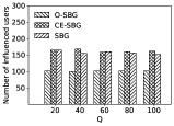
(d) eu-core

Figure 10. Number of influenced users with varying $Q$

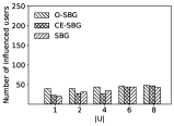
(a) mathoverflow

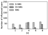
(b) ask-ubuntu

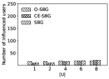
(c) CollegeMsg

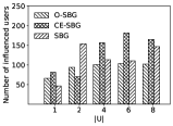
(d) eu-core

Figure 11. Number of influenced users with varying $|\mathcal{U}|$

(a) mathoverflow

(b) ask-ubuntu

(c) CollegeMsg

(d) eu-core

Figure 12. Number of influenced users with varying $l$

7. Related Work

7.1. Influence Maximization

Influence maximization (IM) was first formulated by Domingos et al. (Domingos and Richardson, 2001) as an algorithmic problem in probabilistic methods. Later on, Kempe et al. (Kempe et al., 2003) modeled IM as an algorithmic problem in 2003. As the IM problem is NP-hard, all existing methods focus on approximate solutions, and a keystone of these algorithmic IM studies is the greedy framework. The existing IM algorithms can be categorized into three categories: simulation-based, proxy-based, and sketch-based.

Simulation-based approaches. The key idea of these approaches is to estimate the influence spread $I(S)$ of given users set $S$ by using the Monte Carlo (MC) simulations of the diffusion process (Kempe et al., 2003; Leskovec et al., 2007; Zhou et al., 2015). Specifically, for a given users set $S$, the simulation-based approaches simulate the randomized diffusion process with $S$ for $R$ times. Each time they count the number of active users after the diffusion ends, and then take the average of these counts over the $R$ times. The accuracy of these approaches is positively associated with the number of $R$. The simulation-based approaches have the advantage of diffusion model generality, and these approaches can be incorporated into any classical influence diffusion model. However, the time complexity of these approaches are cost-prohibitive, which would hardly be used for dealing with sizeable networks.

Proxy-based approaches. Instead of running heavy MC simulation, the proxy-based approaches estimate the influence spread of given users by using the proxy models. Intuitively, there are two branches of the proxy-based approaches, including (1) Estimate the influence spread of given users by transforming it to easier problems (e.g., Degree and PageRank) (Chen et al., 2010; Galhotra et al., 2016); and (2) Simplify the typical diffusion model (e.g., IC model) to a deterministic model (e.g., MIA model) (Chen et al., 2010) or restrict the influence propagation range of given users under the typical diffusion model to the local subgraph (Goyal et al., 2011), to precisely compute the influence spread of given users. Compared with the simulation-based approach, a proxy-based approach offers significant performance improvements but lacks theoretical guarantees.

Sketch-based approaches. To avoid running heavy MC simulations and reserve the theoretical guarantee, the sketch-based approaches (Borgs et al., 2014; Tang et al., 2014a; Nguyen et al., 2017; Cohen et al., 2014; Cheng et al., 2013; Ohsaka et al., 2014) pre-compute a number of sketches under a specific diffusion model, and then speed up the influence evaluation based on the constructed sketches. Compared with the simulation-based approaches, the sketch-based approaches have a lower time complexity under a theoretical guarantee. Unfortunately, the sketch-based approaches are not generic to all diffusion models because the generated sketches of the sketch-based approaches are relay on the underlying diffusion models.

7.2. Link Prediction

Link prediction (LP) is an important network-related problem, first proposed by Liben-Nowell et al. (Liben-Nowell and Kleinberg, 2003). The LP problem aims to infer the existence of new links or still unknown interactions between pairs of nodes based on the currently observed links. After decades study, a series of LP methods were proposed, including: similarity approaches (Zhou et al., 2021; He et al., 2015), probabilistic approaches (Das and Das, 2017; Wang et al., 2017), hybrid approaches (Wang et al., 2018; Zhang et al., 2020b), and deep learning approaches (Rahman et al., 2018; Zhang and Chen, 2018; Zhang et al., 2021b).

In this paper, we use the SEAL method (Zhang and Chen, 2018; Zhang et al., 2021b) to predict the structure of the near future (i.e., time point $t$) snapshot graph (i.e., $G_{t}$) for a given evolving graph. Furthermore, for each given users group $\mathcal{U}$, our RT$l$R query problem aims to reconnect a set of edges in $G_{t}$ to maximize the number of influenced users of $\mathcal{U}$ in $G_{t}$, which is quite distinct from all existing IM works.

8. Conclusion

In this paper, we studied the problem of Reconnecting Top-$l$ Relationships (RT$l$R), which aims to find $l$ previous existing relationships but being estranged subsequently, such that reconnecting these relationships would maximize the influence spread of given users group. We have shown that the RT$l$L query problem is NP-hard. We developed a FI-Sketch based greedy (SBG) algorithm to solve this problem. We further devised an edge reducing method to prune the candidate edges that the given users’ group cannot reach. Moreover, an order-based SBG method has been designed by utilizing the submodular characteristic of the RT$l$L query and two well-designed upper bounds. Lastly, the extensive performance evaluations on real datasets also revealed the practical efficiency and effectiveness of our proposed method. In the future, we will focus on developing more efficient approaches to deal with the RT$l$R queries in hyper scale networks.

References

- (1)
- Arora et al. (2017) Akhil Arora, Sainyam Galhotra, and Sayan Ranu. 2017. Debunking the myths of influence maximization: An in-depth benchmarking study. In SIGMOD. 651–666.
- Becker et al. (2020) Ruben Becker, Federico Corò, Gianlorenzo D’Angelo, and Hugo Gilbert. 2020. Balancing spreads of influence in a social network. In AAAI. 3–10.
- Borgs et al. (2014) Christian Borgs, Michael Brautbar, Jennifer T. Chayes, and Brendan Lucier. 2014. Maximizing Social Influence in Nearly Optimal Time. In SODA. 946–957.
- Brown and Reingen (1987) Jacqueline Johnson Brown and Peter H Reingen. 1987. Social ties and word-of-mouth referral behavior. Journal of Consumer research 14, 3 (1987), 350–362.
- Cai et al. (2022) Taotao Cai, Jianxin Li, Ajmal Mian, Rong-Hua Li, Timos Sellis, and Jeffrey Xu Yu. 2022. Target-Aware Holistic Influence Maximization in Spatial Social Networks. IEEE Trans. Knowl. Data Eng. 34, 4 (2022), 1993–2007.
- Chen et al. (2010) Wei Chen, Chi Wang, and Yajun Wang. 2010. Scalable influence maximization for prevalent viral marketing in large-scale social networks. In SIGKDD. 1029–1038.
- Chen et al. (2020) Wei Chen, Weizhong Zhang, and Haoyu Zhao. 2020. Gradient Method for Continuous Influence Maximization with Budget-Saving Considerations. In AAAI. 43–50.
- Chen et al. (2015) Xiaodong Chen, Guojie Song, Xinran He, and Kunqing Xie. 2015. On Influential Nodes Tracking in Dynamic Social Networks. In SIAM, Suresh Venkatasubramanian and Jieping Ye (Eds.). 613–621.
- Cheng et al. (2013) Suqi Cheng, Huawei Shen, Junming Huang, Guoqing Zhang, and Xueqi Cheng. 2013. StaticGreedy: Solving the Scalability-Accuracy Dilemma in Influence Maximization. In CIKM. 509–518.
- Cohen et al. (2014) Edith Cohen, Daniel Delling, Thomas Pajor, and Renato F. Werneck. 2014. Sketch-Based Influence Maximization and Computation: Scaling up with Guarantees. In CIKM. 629–638.
- Das et al. (2019) Apurba Das, Michael Svendsen, and Srikanta Tirthapura. 2019. Incremental maintenance of maximal cliques in a dynamic graph. The VLDB Journal 28, 3 (2019), 351–375.
- Das and Das (2017) Sima Das and Sajal K Das. 2017. A probabilistic link prediction model in time-varying social networks. In 2017 IEEE International Conference on Communications (ICC). 1–6.
- Domingos and Richardson (2001) Pedro Domingos and Matt Richardson. 2001. Mining the network value of customers. In SIGMOD. 57–66.
- Feng et al. (2014) Shanshan Feng, Xuefeng Chen, Gao Cong, Yifeng Zeng, Yeow Meng Chee, and Yanping Xiang. 2014. Influence Maximization with Novelty Decay in Social Networks. In AAAI. 37–43.
- Galhotra et al. (2016) Sainyam Galhotra, Akhil Arora, and Shourya Roy. 2016. Holistic influence maximization: Combining scalability and efficiency with opinion-aware models. In ICDM. 743–758.
- Goyal et al. (2011) Amit Goyal, Wei Lu, and Laks VS Lakshmanan. 2011. Simpath: An efficient algorithm for influence maximization under the linear threshold model. In ICDM. 211–220.
- Guo et al. (2013) Jing Guo, Peng Zhang, Chuan Zhou, Yanan Cao, and Li Guo. 2013. Personalized influence maximization on social networks. In CIKM. 199–208.
- He et al. (2015) Yu-lin He, James NK Liu, Yan-xing Hu, and Xi-zhao Wang. 2015. OWA operator based link prediction ensemble for social network. Expert Systems with Applications 42, 1 (2015), 21–50.
- Hoeffding (1963) Wassily Hoeffding. 1963. Probability Inequalities for Sums of Bounded Random Variables. J. Amer. Statist. Assoc. 58, 301 (1963), 13–30.
- Huang et al. (2019) Shixun Huang, Zhifeng Bao, J Shane Culpepper, and Bang Zhang. 2019. Finding temporal influential users over evolving social networks. In ICDE. 398–409.
- Jia et al. (2021) Xiaowei Jia, Xiaoyi Li, Nan Du, Yuan Zhang, Vishrawas Gopalakrishnan, Guangxu Xun, and Aidong Zhang. 2021. Tracking Community Consistency in Dynamic Networks: An Influence-Based Approach. IEEE Trans. Knowl. Data Eng. 33, 2 (2021), 782–795.
- Karp (1972) Richard M Karp. 1972. Reducibility among combinatorial problems. In Complexity of Computer Computations. 85–103.
- Kempe et al. (2003) David Kempe, Jon M. Kleinberg, and Éva Tardos. 2003. Maximizing the spread of influence through a social network. In SIGKDD. 137–146.
- Kempe et al. (2015) David Kempe, Jon M. Kleinberg, and Éva Tardos. 2015. Maximizing the Spread of Influence through a Social Network. Theory Comput. 11 (2015), 105–147.
- Kroese et al. (2014) Dirk P Kroese, Tim Brereton, Thomas Taimre, and Zdravko I Botev. 2014. Why the Monte Carlo method is so important today. Wiley Interdiscip Rev Comput Stat 6, 6 (2014), 386–392.
- Leskovec et al. (2008) Jure Leskovec, Lars Backstrom, Ravi Kumar, and Andrew Tomkins. 2008. Microscopic evolution of social networks. In SIGKDD. 462–470.
- Leskovec et al. (2007) Jure Leskovec, Andreas Krause, Carlos Guestrin, Christos Faloutsos, Jeanne VanBriesen, and Natalie Glance. 2007. Cost-effective outbreak detection in networks. In SIGKDD. 420–429.
- Li et al. (2020) Jianxin Li, Taotao Cai, Ke Deng, Xinjue Wang, Timos Sellis, and Feng Xia. 2020. Community-diversified influence maximization in social networks. Inf. Syst. 92 (2020), 101522.
- Li et al. (2017) Yuchen Li, Ju Fan, Dongxiang Zhang, and Kian-Lee Tan. 2017. Discovering your selling points: Personalized social influential tags exploration. In ICDM. 619–634.
- Li et al. (2015) Yuchen Li, Dongxiang Zhang, and Kian-Lee Tan. 2015. Real-time Targeted Influence Maximization for Online Advertisements. In PVLDB. 1070–1081.
- Liben-Nowell and Kleinberg (2003) David Liben-Nowell and Jon M. Kleinberg. 2003. The link prediction problem for social networks. In CIKM. 556–559.
- Lu et al. (2015) Wei Lu, Wei Chen, and Laks VS Lakshmanan. 2015. From competition to complementarity: comparative influence diffusion and maximization. arXiv preprint arXiv:1507.00317 (2015).
- Nguyen et al. (2017) Hung T Nguyen, Tri P Nguyen, NhatHai Phan, and Thang N Dinh. 2017. Importance sketching of influence dynamics in billion-scale networks. In ICDM. 337–346.
- Nguyen et al. (2016) Hung T Nguyen, My T Thai, and Thang N Dinh. 2016. Stop-and-stare: Optimal sampling algorithms for viral marketing in billion-scale networks. In SIGMOD. 695–710.
- Ohsaka et al. (2014) Naoto Ohsaka, Takuya Akiba, Yuichi Yoshida, and Ken-ichi Kawarabayashi. 2014. Fast and accurate influence maximization on large networks with pruned monte-carlo simulations. In AAAI.
- Ou et al. (2016) Han-Ching Ou, Chung-Kuang Chou, and Ming-Syan Chen. 2016. Influence maximization for complementary goods: Why parties fail to cooperate?. In CIKM. 1713–1722.
- Ou et al. (2022) Jiamin Ou, Vincent Buskens, Arnout van de Rijt, and Debabrata Panja. 2022. Influence maximization under limited network information: Seeding high-degree neighbors. CoRR abs/2202.03893 (2022).
- Rahman et al. (2018) Mahmudur Rahman, Tanay Kumar Saha, Mohammad Al Hasan, Kevin S Xu, and Chandan K Reddy. 2018. Dylink2vec: Effective feature representation for link prediction in dynamic networks. arXiv preprint arXiv:1804.05755 (2018).
- Singh and Kailasam (2021) Ashwini Kumar Singh and Lakshmanan Kailasam. 2021. Link prediction-based influence maximization in online social networks. Neurocomputing 453 (2021), 151–163.
- Tang et al. (2014a) Youze Tang, Xiaokui Xiao, and Yanchen Shi. 2014a. Influence maximization: Near-optimal time complexity meets practical efficiency. In SIGMOD. 75–86.
- Tang et al. (2014b) Youze Tang, Xiaokui Xiao, and Yanchen Shi. 2014b. Influence maximization: near-optimal time complexity meets practical efficiency. In SIGMOD. 75–86.
- Tsang et al. (2019) Alan Tsang, Bryan Wilder, Eric Rice, Milind Tambe, and Yair Zick. 2019. Group-Fairness in Influence Maximization. In IJCAI. 5997–6005.
- Tsaras et al. (2021) Dimitris Tsaras, George Trimponias, Lefteris Ntaflos, and Dimitris Papadias. 2021. Collective Influence Maximization for Multiple Competing Products with an Awareness-to-Influence Model. Proc. VLDB Endow. 14, 7 (2021), 1124–1136.
- Wang et al. (2017) Tong Wang, Xing-Sheng He, Ming-Yang Zhou, and Zhong-Qian Fu. 2017. Link prediction in evolving networks based on popularity of nodes. Scientific Reports 7, 1 (2017), 1–10.
- Wang et al. (2010) Yu Wang, Gao Cong, Guojie Song, and Kunqing Xie. 2010. Community-based greedy algorithm for mining top-K influential nodes in mobile social networks. In SIGKDD. 1039–1048.
- Wang et al. (2018) Zhiqiang Wang, Jiye Liang, and Ru Li. 2018. A fusion probability matrix factorization framework for link prediction. Knowledge-Based Systems 159 (2018), 72–85.
- Xie et al. (2015) Miao Xie, Qiusong Yang, Qing Wang, Gao Cong, and Gerard De Melo. 2015. Dynadiffuse: A dynamic diffusion model for continuous time constrained influence maximization. In AAAI. 346–352.
- Yadav et al. (2018) Amulya Yadav, Bryan Wilder, Eric Rice, Robin Petering, Jaih Craddock, Amanda Yoshioka-Maxwell, Mary Hemler, Laura Onasch-Vera, Milind Tambe, and Darlene Woo. 2018. Bridging the gap between theory and practice in influence maximization: Raising awareness about HIV among homeless youth.. In IJCAI. 5399–5403.
- Zhang and Chen (2018) Muhan Zhang and Yixin Chen. 2018. Link prediction based on graph neural networks. Advances in Neural Information Processing Systems 31 (2018), 5165–5175.
- Zhang et al. (2021b) Muhan Zhang, Pan Li, Yinglong Xia, Kai Wang, and Long Jin. 2021b. Labeling Trick: A Theory of Using Graph Neural Networks for Multi-Node Representation Learning. Advances in Neural Information Processing Systems 34 (2021).
- Zhang et al. (2020a) Ping Zhang, Zhifeng Bao, Yuchen Li, Guoliang Li, Yipeng Zhang, and Zhiyong Peng. 2020a. Towards an Optimal Outdoor Advertising Placement: When a Budget Constraint Meets Moving Trajectories. ACM Trans. Knowl. Discov. Data 14, 5 (2020), 1–32.
- Zhang et al. (2020b) Qi Zhang, Tingting Tong, and Shunyao Wu. 2020b. Hybrid link prediction via model averaging. Physica A: Statistical Mechanics and its Applications 556 (2020), 124772.
- Zhang et al. (2021a) Yipeng Zhang, Yuchen Li, Zhifeng Bao, Baihua Zheng, and HV Jagadish. 2021a. Minimizing the Regret of an Influence Provider. In SIGMOD. 2115–2127.
- Zhou et al. (2015) Chuan Zhou, Peng Zhang, Wenyu Zang, and Li Guo. 2015. On the upper bounds of spread for greedy algorithms in social network influence maximization. IEEE Trans. Knowl. Data. Eng. 27, 10 (2015), 2770–2783.
- Zhou et al. (2021) Tao Zhou, Yan-Li Lee, and Guannan Wang. 2021. Experimental analyses on 2-hop-based and 3-hop-based link prediction algorithms. Physica A: Statistical Mechanics and Its Applications 564 (2021), 125532.
- Zhu et al. (2016) Linhong Zhu, Dong Guo, Junming Yin, Greg Ver Steeg, and Aram Galstyan. 2016. Scalable Temporal Latent Space Inference for Link Prediction in Dynamic Social Networks. IEEE Trans. Knowl. Data. Eng. 28, 10 (2016), 2765–2777.