Temporally coherent backmapping of molecular trajectories from coarse-grained to atomistic resolution

Abstract

Coarse-graining offers a means to extend the achievable time and length scales of molecular dynamics simulations beyond what is practically possible in the atomistic regime. Sampling molecular configurations of interest can be done efficiently using coarse-grained simulations, from which meaningful physicochemical information can be inferred if the corresponding all-atom configurations are reconstructed. However, this procedure of backmapping to reintroduce the lost atomistic detail into coarse-grain structures has proven a challenging task due to the many feasible atomistic configurations that can be associated with one coarse-grain structure. Existing backmapping methods are strictly frame-based, relying on either heuristics to replace coarse-grain particles with atomic fragments and subsequent relaxation, or parameterized models to propose atomic coordinates separately and independently for each coarse-grain structure. These approaches neglect information from previous trajectory frames that is critical to ensuring temporal coherence of the backmapped trajectory, while also offering information potentially helpful to produce higher-fidelity atomic reconstructions. In this work we present a deep learning-enabled data-driven approach for temporally coherent backmapping that explicitly incorporates information from preceding trajectory structures. Our method trains a conditional variational autoencoder to non-deterministically reconstruct atomistic detail conditioned on both the target coarse-grain configuration and the previously reconstructed atomistic configuration. We demonstrate our backmapping approach on two exemplar biomolecular systems: alanine dipeptide and the miniprotein chignolin. We show that our backmapped trajectories accurately recover the structural, thermodynamic, and kinetic properties of the atomistic trajectory data.

Department of Physics, Freie Universität Berlin, Berlin, Germany

1 Introduction

A central limitation of modelling soft-matter systems with molecular dynamics (MD) simulations are the long characteristic timescales of interesting processes, such as protein folding, compared to the relatively short integration time steps required to accurately propagate the system forward in time. A plethora of strategies strive to overcome this time scale barrier, such as enhanced sampling techniques, ^{1, 2, 3, 4, 5} modern/specialized hardware, ^{6, 7, 8} and hierarchical multiscale modelling ^{9, 10, 11, 12, 13, 14}. Coarse-grained (CG) simulations are one such multiscale approach that enables access to spatiotemporal scales entirely out of reach of conventional atomistic molecular dynamics simulations. The process of coarse-graining typically aggregates groups of atoms into ‘beads’ or ‘superatoms’ intended to preserve important properties of the original atomistic system ^{15, 16, 17}. As such, CG simulations require monitoring fewer particles which allows for the study of larger and more complex systems typically untenable in the atomistic regime at comparable computational cost. A typical consequence of this reduction in resolution is an effective ‘smoothing’ of the underlying free energy surface, which helps expedite large-scale and slowly evolving conformational motions that might otherwise be frustrated or kinetically trapped in the more rugged atomistic landscape ^{18, 19, 12, 20, 21} These advantages have led to the growing popularization and use of CG models particularly for simulations of proteins, polymers, molecular self-assembly, membranes, and high-throughput screening ^{22, 23, 24, 25, 26, 27, 28, 29, 30, 31}.

The primary concession of coarse-graining is the sacrifice of fine-grained, atomistic detail. Restoring this lost detail by converting a CG representation into a corresponding atomistic representation is commonly dubbed “backmapping” and is important for analyses requiring atomistic resolution, for example electronic structure calculations for determining NMR spectra or dipole moments ^{32, 33}. A major difficulty of backmapping is the inherent ambiguity of many atomistic structures that are feasible candidates to a singular CG configuration. Traditional backmapping strategies rely on geometric heuristics to replace beads with their associated atomic fragments. These approaches typically produce quite poor initial structures that must be subsequently subjected to refinement using energy minimization and/or (restrained) molecular dynamics to equilibrate each backmapped frame ^{11, 34, 35, 36, 37}. However, significant computational cost is incurred with the required frame-by-frame intervention in these approaches which hinders the applicability of backmapping larger systems and/or longer trajectories. More recently, data-driven backmapping techniques have been proposed which deploy machine learning (ML) models that learn to reconstruct atomistic details from training examples ^{38, 39, 40, 41, 42, 43}. These approaches offer more scalability with higher throughput as they are typically trained to produce well-equilibrated structures that do not require frame-by-frame energy minimization or relaxation. Coarse-graining is an inherently many-to-one operation, with multiple atomic structures corresponding to each CG representation. A favorable feature of any backmapping procedure is the capacity to recapitulate the conformational diversity of atomic structures corresponding to a particular CG representation. A subset of these data-driven methods  ^{38, 39, 43, 41} that possess this conformational expressibility are therefore capable of non-deterministic backmapping, where a variety of feasible and novel atomistic structures can be generated when backmapping any individual CG configuration.

A commonality between all existing approaches is backmapping each frame individually and separately from one-another. However, leveraging temporal information can improve reconstruction quality and enable the recovery of dynamic properties. In particular, some important dynamic properties rely on time correlations of local atomistic details. For example, the calculation of diffusion constants is related to the integral of the velocity auto-correlation ⁴⁴, infrared absorption spectra is related to the auto-correlation function of the total dipole moment ^{45, 46}, and scattering functions that are related to Fourier transforms of the van Hove correlation function ^{47, 48, 49, 50}. Existing backmapping schemes are not temporally aware and correlations between consecutive frames are only maintained via large-scale characteristics. As a consequence, the reintroduced degrees of freedom between consecutive frames might decorrelate locally, and time correlations based on local, atomistic descriptors are typically not reliable for such backmapped trajectories. Therefore, presently absent from this suite of backmapping methods is a data-driven approach for generatively backmapping CG trajectories that also incorporates temporal information.

We present in this work a new method to perform temporally coherent backmapping of molecular simulation trajectories via a deep learning-based solution for all-atom reconstruction of CG simulation trajectories that aims at both generating well-equilibrated molecular structures for each frame and achieves temporal coherence between frames. To this end, we explicitly incorporate configurational information from previous simulation frames when generating reconstructions. This task is accomplished by training a conditional variational autoencoder (cVAE) that learns to up-scale CG configurations into full atomistic resolution by conditioning on the current coarse- and previous fine-grained structures. Our cVAE learns to model a variety of feasible atomistic structures associated with each CG configuration, which allows us to generatively produce novel backmapped trajectories that are not a simple carbon copy of the training data. We show for two exemplar biomolecular systems alanine dipeptide (ADP) and the miniprotein chignolin (CLN) that our approach generates atomic reconstructions which recover atomistic structural, thermodynamic, and kinetic properties. Furthermore, we show our backmapping model performs well on held out in distribution data and generalizes to CG data originating from unseen and approximate CG force fields.

2 Methods

Our approach utilizes a reference atomistic trajectory (or set of atomistic trajectories) for a molecule we intend to backmap. The trajectory contains $N$ atoms and is composed of a collection of $T$ frames $\mathbf{AA}=\{{\mathrm{AA}}^{0},{\mathrm{AA}}^{1},\ldots,{\mathrm{AA}}^{T-1}\}$, where ${\mathrm{AA}}^{t}\in\mathbb{R}^{N\times 3}$ are the atomistic coordinates for each frame. We assume there exists a coarse-graining function $f_{cg}$ that maps all-atom coordinates to CG coordinates, such that $f_{cg}({\mathrm{AA}}^{t})={\mathrm{CG}}^{t}\in\mathbb{R}^{n\times 3}$, where $n$ is the number CG beads such that $n<N$. This function is then applied frame-by-frame to the atomistic frames $\mathbf{AA}$ yielding the corresponding CG trajectory $\mathbf{CG}=\{{\mathrm{CG}}^{0},{\mathrm{CG}}^{1},\ldots,{\mathrm{CG}}^{T-1}\}$. This pair of atomistic and CG trajectories $(\mathbf{AA},\mathbf{CG})$ compose the data used to train our super-resolution model (Fig. 1a). From this data our model attempts to learn the conditional distribution $P({\mathrm{AA}}^{t}|{\mathrm{CG}}^{t},{\mathrm{AA}}^{t-1})$ implicitly, such that we can reconstruct an atomisitic configuration given the CG structure ${\mathrm{CG}}^{t}$ and a previous atomistic structure ${\mathrm{AA}}^{t-1}$. Each training sample therefore consists of a sequential pair of atomistic configurations and the current CG configuration $({\mathrm{AA}}^{t},{\mathrm{CG}}^{t},{\mathrm{AA}}^{t-1})$. While increasing the number of previous frames to incorporate ${\mathrm{AA}}^{t-2},{\mathrm{AA}}^{t-3},\ldots$ is straight-forward, our experiments show that this simpler Markovian posture already yields accurate temporally coherent reconstructions that reproduce structural, thermodynamic and kinetic properties with remarkable accuracy. A complete PyTorch ⁵¹ implementation of our model with all associated analyses is publically available at DOI:10.18126/tf0h-w0jz ⁵².

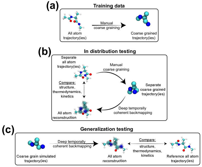
Figure 1: Illustration of training and testing setups.

2.1 Representing molecules as spatially voxelized particle densities

Learning complex and high-order dependencies is a hallmark of computer vision. One of the most successful generative models are convolutional neural networks (CNNs), which have led to groundbreaking successes in image processing ^{53, 54, 55, 56, 57}. In order to take advantage of CNNs for our backmapping task we choose to represent our data as a set of 3D featurized images. To this end, a smooth density representation discretized on a 3D grid is used to encode the positions of atoms and beads. Each particle is placed in a separate tensor channel to avoid overlap of densities that would be difficult to disentangle. More concretely, an atomistic configuration ${\mathrm{AA}}^{t}\in\mathbb{R}^{N\times 3}$ is represented as a 4D tensor ${\mathrm{VOX}}^{{\mathrm{AA}}^{t}}\in\mathbb{R}^{d\times d\times d\times N}$, where the first three dimensions discretize the location of each particle in space and the final dimension represents a channel for each particle:

$${\mathrm{VOX}}^{{\mathrm{AA}}_{t}}_{i}(\mathbf{x})=\exp\left(-\frac{(\mathbf{x}-{\mathrm{AA}}^{t}_{i})^{2}}{2\sigma^{2}}\right).$$ (1)

Here, $i$ is the particle index and $\mathbf{x}\in\mathbb{R}^{3}$ is the Cartesian location of each grid point taken from a regular Cartesian grid of width $r_{grid}$ such that the maximal and minimal values of each spatial dimension are $-\frac{r_{grid}}{2}$ and $\frac{r_{grid}}{2}$. The density of each particle is therefore a 3D Gaussian centered about the position ${\mathrm{AA}}_{i}^{t}\in\mathbb{R}^{3}$ with the width $\sigma$. It is critical to ensure $r_{grid}$ is large enough such that each particle density within the trajectory is fully enclosed by the voxelized grid. The parameter $d$ then controls the resolution of our spatial discretization, such that a larger $d$ leads to more spatial resolution at the cost of higher memory and processing requirements. Furthermore, $\sigma$, which controls the effective size of each particle density, will also impact the mass assigned to each voxel.

From a density profile ${\mathrm{VOX}}^{{\mathrm{AA}}^{t}}_{i}$ we can also recover a set of particle coordinates by performing a weighted average over the voxelized grid,

$$\tilde{{\mathrm{AA}}^{t}_{i}}=\frac{1}{z}\sum_{j=1}^{d}\sum_{k=1}^{d}\sum_{l=1}^{d}x_{j,k,l}{\mathrm{VOX}}^{{\mathrm{AA}}^{t}}_{i}(x_{j,k,l})$$ (2)

where $z=\sum_{j=1}^{d}\sum_{k=1}^{d}\sum_{l=1}^{d}{\mathrm{VOX}}^{{\mathrm{AA}}^{t}}_{i}(x_{j,k,l})$ is a normalization constant, $x_{j,k,l}$ is a particular coordinate value within the three-dimensional spatially voxelized grid and the summations are carried over the three spatial dimensions. Given a predicted density profile ${\mathrm{VOX}}^{\hat{{\mathrm{AA}}}^{t}}$ we can perform this weighted average for each $i$ particle channel ${\mathrm{VOX}}^{\hat{{\mathrm{AA}}}^{t}}_{i}$ to recover the complete set of atomistic coordinates $\hat{{\mathrm{AA}}^{t}}$. We note that transforming these densities into and from Cartesian coordinates constitutes a sequence of differentiable operations and therefore enables us to readily incorporate this particle averaging and voxelization within the computational graph of our model. CG configurations ${\mathrm{CG}}^{t}$ are treated in the same way as their atomistic counter-parts, yielding corresponding voxelized representations ${\mathrm{VOX}}^{{\mathrm{CG}}^{t}}\in\mathbb{R}^{d\times d\times d\times n}$ where $n$ is the number of beads associated with each CG configuration.

2.2 Conditional Variational Autoencoder

To learn a temporally coherent probabilistic mapping from CG to atomistic configurations we train a conditional variational autoencoder (cVAE) ⁵⁸. A typical VAE ⁵⁹ consists of an encoder that compresses high-dimensional inputs into a lower dimensional latent space that captures salient information characterizing the input data. This latent, compressed representation is then inputted to a decoder that aims to reconstruct the original high-dimensional input. The cVAE operates under a similar premise but the decoder is also provided with some partial information about the input along with the latent code when producing reconstructions. Fig. 2a shows a schematic illustration of our cVAE architecture. In our application, the cVAE encoder takes as input the triplet of configurations $({\mathrm{AA}}^{t},{\mathrm{CG}}^{t},{\mathrm{AA}}^{t-1})$, where the subset $({\mathrm{CG}}^{t},{\mathrm{AA}}^{t-1})$ is interpreted as the conditional variable and ${\mathrm{AA}}^{t}$ the intended reconstruction target. The decoder is a function of both the latent code and the conditional variable $({\mathrm{CG}}^{t},{\mathrm{AA}}^{t-1})$ and learns to reconstruct atomistic configurations $\hat{{\mathrm{AA}}^{t}}$ to closely match the data ${\mathrm{AA}}^{t}$. For a fixed condition $({\mathrm{CG}}^{t},{\mathrm{AA}}^{t-1})$ we can learn to meaningfully encode information about the target configuration ${\mathrm{AA}}^{t}$ into a low dimensional latent code, such that the decoder when presented with $({\mathrm{CG}}^{t},{\mathrm{AA}}^{t-1})$ yields slightly different, yet valid, reconstructions $\hat{\AA^{t}}$ for different instantiations of the latent code. This data driven approach enables our model to generatively produce reconstructions ${\mathrm{AA}}^{t}$ in a temporally aware way by conditioning on both the coarse grained configuration and the previous atomistic configuration $({\mathrm{CG}}^{t},{\mathrm{AA}}^{t-1})$ (Fig. 2b).

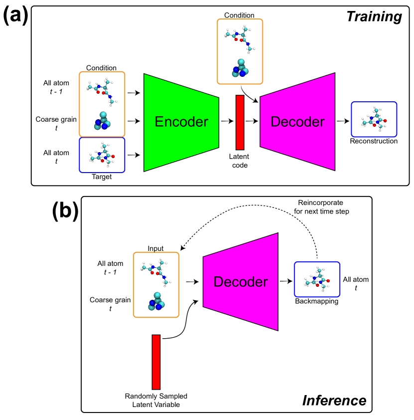
Figure 2: Schematic illustration of our model training and inference setups.

2.2.1 The Encoder

The purpose of the encoder in our cVAE is to distill information from the input configurations $({\mathrm{AA}}^{t},{\mathrm{CG}}^{t},{\mathrm{AA}}^{t-1})$ into a low-dimensional latent space vector that is used in conjunction with the conditional variables $({\mathrm{CG}}^{t},{\mathrm{AA}}^{t-1})$ for the decoder to generate an atomistic reconstruction $\hat{{\mathrm{AA}}}^{t}$. These configurations are passed to the encoder as voxelized grids of particle densities $({\mathrm{VOX}}^{{\mathrm{AA}}^{t}},{\mathrm{VOX}}^{{\mathrm{CG}}^{t}},{\mathrm{VOX}}^{{\mathrm{AA}}^{t-1}})$ which are constructed as a single monolithic tensor concatenated along the particle dimension $\mathbf{x}=[{\mathrm{VOX}}^{{\mathrm{AA}}^{t}}||{\mathrm{VOX}}^{{\mathrm{CG}}^{t}}||{\mathrm{VOX}}^{{\mathrm{AA}}^{t-1}}]\in\mathbb{R}^{d\times d\times d\times(2N+n)}$, where $N$ and $n$ are the number of atoms/beads in each atomistic and CG configuration, respectively. The encoder is composed of 3D residual CNNs with a terminal dense layer to extract a fixed dimensional latent vector. The locality of the CNN kernel provides a strong inductive bias by focusing on proximate spatial profiles from multiple high and low resolution scales and multiple time steps. Processing the input $\mathbf{x}$ using many consecutive CNN modules enables us to hierarchically incorporate progressively more distant features, and ultimately yielding a multiscale, spatially and temporally aware latent representation $\mathbf{z}\in d_{\text{latent}}$ for that slice of the trajectory. This latent representation $\mathbf{z}$ is then passed to the decoder in conjunction with the conditional variable $\mathbf{c}=[{\mathrm{VOX}}^{{\mathrm{CG}}^{t}}||{\mathrm{VOX}}^{{\mathrm{AA}}^{t-1}}]$ to predict the all atom configuration for the subsequent time step $\text{Decoder}(\mathbf{c},\mathbf{z})=\hat{{\mathrm{AA}}^{t}}$.

2.2.2 The Decoder

The purpose of the decoder is to use information provided in the conditional variable $\mathbf{y}=[{\mathrm{VOX}}^{{\mathrm{CG}}^{t}}||{\mathrm{VOX}}^{{\mathrm{AA}}^{t-1}}]$ jointly with the latent code $\mathbf{z}$ produced by the encoder to reconstruct of the current atomistic configuration ${\mathrm{AA}}^{t}$. Upon completing training, we can eschew the encoder and use the decoder as our generative model for backmapping. Using a randomly sampled latent variable $\mathbf{z}$ as a source of noise while specifying the conditional variable as the current CG configuration ${\mathrm{CG}}^{t}$ and the previous atomistic configuration ${\mathrm{AA}}^{t-1}$ we can backmap the atomistic reconstruction $\hat{{\mathrm{AA}}^{t}}$. Similar to the encoder, our decoder is primarily composed of residual 3D CNNs. Unlike the encoder, the neural network backbone of the decoder needs to only output a 4D tensor of equivalent dimensionality to the voxelized atomistic representation ${\mathrm{VOX}}^{{\mathrm{AA}}^{t}}\in\mathbb{R}^{d\times d\times d\times N}$. As the voxelized representation ${\mathrm{VOX}}^{{\mathrm{AA}}^{t}}$ contains separate channels for each atom, we can simply perform an average over of the spatial density profiles within each particle channel to independently localize each atom coordinate (c.f. Sec. 2.1). We control the behavior of our model by defining a training loss that captures relevant aspects we ultimately want reflected in our reconstructions.

2.3 Training routines

Our model is trained end-to-end using the ADAM optimizer ⁶⁰. For a single sample, the complete loss $\mathcal{L}$ is given by

$$\mathcal{L} =\mathcal{L}_{{\mathrm{VOX}}}+\mathcal{L}_{{\mathrm{AA}}}+\mathcal{L}_{\text{CG}}+\mathcal{L}_{\text{EDM}}+\lambda\mathcal{L}_{\text{ENERGY}}+\beta\mathcal{L}_{\text{KLD}}$$ (3)

$$\mathcal{L}_{{\mathrm{VOX}}} =\frac{1}{d^{3}N}\ ||{\mathrm{VOX}}^{{\mathrm{AA}}^{t}}-{\mathrm{VOX}}^{\hat{{\mathrm{AA}}^{t}}}||_{F}^{2}$$

$$\mathcal{L}_{{\mathrm{AA}}} =\frac{1}{3N}\ ||{\mathrm{AA}}^{t}-\hat{{\mathrm{AA}}^{t}}||_{F}^{2}$$

$$\mathcal{L}_{\text{CG}} =\frac{1}{3n}\ ||{\mathrm{CG}}^{t}-\hat{{\mathrm{CG}}^{t}}||_{F}^{2}$$

$$\mathcal{L}_{\text{EDM}} =\frac{1}{2N^{2}}\ ||EDM^{{\mathrm{AA}}^{t}}-EDM^{\hat{{\mathrm{AA}}^{t}}}||_{F}^{2}$$

$$\mathcal{L}_{\text{ENERGY}} =(U^{{\mathrm{AA}}^{t}}-U^{\hat{{\mathrm{AA}}^{t}}})^{2}$$

$$\mathcal{L}_{\text{KLD}} =\mathcal{D}_{KL}(\mathbf{z}||\mathcal{N}(0,\mathbf{I})).$$

The first five terms in Eqn. 3 are components of an effective reconstruction loss and $\mathcal{L}_{\text{KLD}}$ is the standard Kullback–Leibler divergence loss between the latent code $\mathbf{z}$ and a normal distribution typically used in VAE training ⁵⁹. While we ultimately strive to recover all atom coordinates ${\mathrm{AA}}^{t}$, the model primarily operates on spatially voxelized particle densities representations ${\mathrm{VOX}}^{{\mathrm{AA}}^{t}}$. A critical component of learning will therefore involve reconstructing these density profiles to enable accurate and sharp atomic coordinate generation. The $\mathcal{L}_{{\mathrm{VOX}}}$ term is a mean squared error (MSE) between the target ${\mathrm{VOX}}^{{\mathrm{AA}}^{t}}$ and reconstructed ${\mathrm{VOX}}^{\hat{{\mathrm{AA}}^{t}}}$ atomistic voxels, while $\mathcal{L}_{{\mathrm{AA}}}$ is an MSE between the ground truth ${\mathrm{AA}}^{t}$ and reconstructed $\hat{{\mathrm{AA}}^{t}}$ atomic coordinates. $\mathcal{L}_{{\mathrm{VOX}}}$ helps the model learn to reproduce the atomic densities of the intermediate voxelized representations, while $\mathcal{L}_{{\mathrm{AA}}}$ helps ensure sharper coordinate reconstruction when the voxels ${\mathrm{VOX}}^{{\mathrm{AA}}^{t}}$ are ultimately collapsed back into atomic coordinates ${\mathrm{AA}}^{t}$. We also use the coarse graining function $f_{cg}$ to determine the CG representation of an atomistic reconstruction $\hat{{\mathrm{CG}}^{t}}=f_{cg}(\hat{{\mathrm{AA}}^{t}})$, which is used in $\mathcal{L}_{\text{CG}}$ to calculate an MSE with respect to the input CG coordinates ${\mathrm{CG}}^{t}$. The motivation to include $\mathcal{L}_{\text{CG}}$ is that a coarse graining of the atomistic backmapping $\hat{{\mathrm{AA}}^{t}}$ should ultimately match the original CG structure ${\mathrm{CG}}^{t}$ from which the reconstruction is derived. In the $\mathcal{L}_{\text{EDM}}$ term we calculate an MSE between the $N\times N$-dimensional Euclidean Distance Matrix (EDM) of the target $EDM^{{\mathrm{AA}}^{t}}$ and the reconstructed $EDM^{\hat{{\mathrm{AA}}^{t}}}$ atomic coordinates to help our backmapping better preserve bond lengths and other interatomic distances. Lastly, in the $\mathcal{L}_{\text{ENERGY}}$ term we calculate an MSE between the scalar valued total potential energy of the target $U^{{\mathrm{AA}}^{t}}$ and reconstruction $U^{\hat{{\mathrm{AA}}^{t}}}$. $\mathcal{L}_{\text{ENERGY}}$ serves as a regularizer to improve the quality of backmapped structures by penalizing reconstructed configurations that may have suitable geometric contributions but are otherwise energetically unfavorable. As such, it accelerates convergence and helps more precisely match the reconstructed energetics to the ground truth trajectory. During training, before configurations are voxelized, each training configuration is mean centered and we learn covariance with respect to rigid rotations by applying a random Euler rotation $\mathbf{R}\in\mathbb{R}^{3\times 3}$ separately augmenting samples in each forward pass $({\mathrm{AA}}^{t},{\mathrm{CG}}^{t},{\mathrm{AA}}^{t-1})\rightarrow({\mathrm{AA}}^{t}\mathbf{R},{\mathrm{CG}}^{t}\mathbf{R},{\mathrm{AA}}^{t-1}\mathbf{R})$.

A challenge of incorporating $\mathcal{L}_{\text{ENERGY}}$ within the loss function is that the potential energy function $U$ is sensitive to small perturbations of the atomic coordinates, which is most severe for the bonded and non-bonded Lennard-Jones interaction. As such, it can become dominatingly large during the early stages of training before the model learns to stably localize atomic coordinates. To alleviate this issue, we incorporate the prefactor $\lambda$ in Eqn. 3 which we set to $\lambda=0$ for a fixed number of initial training steps after which point $\lambda$ is slowly annealed up to $\lambda=1$ using an exponential annealing schedule. We also include the $\beta$ prefactor alongside $\mathcal{L}_{\text{KLD}}$ for more flexibility in balancing the impact of the KL regularization against the reconstruction losses. For the ADP model we employ a cyclic annealing schedule for $\beta$ to mitigate KL vanishing ⁶¹, while for the CLN model we simply maintain $\beta=1$ throughout training. Complete training settings and hyperparameter details are presented in the Supporting Information.

2.4 Inference

At inference time, we omit the encoder and use the decoder as the primary tool for generatively backmapping a CG trajectory. The decoder thereby reconstructs the atomistic frames in an autoregressive manner, i.e., the previous reconstructed atomistic frame $\hat{{\mathrm{AA}}^{t-1}}$ serves as the input for the reconstruction of the next frame $\hat{{\mathrm{AA}}^{t}}$. More specifically, the input for the decoder consists of a fixed dimensional latent vector $\mathbf{z}$ and the conditional variable $\mathbf{c}=[{\mathrm{VOX}}^{{\mathrm{CG}}^{t}}||{\mathrm{VOX}}^{{\mathrm{AA}}^{t-1}}]$ (Fig. 2b). However, for the first trajectory frame $t=0$ there is no preceding frame for us to ascertain ${\mathrm{AA}}^{-1}$. In this case, an atomistic configuration from the training dataset is chosen as this initial seed configuration ${\mathrm{AA}}^{-1}$. We select this configuration by first determining the trajectory frame $t^{*}$ in the training dataset ${\mathrm{AA}}_{\text{train}}$ that minimizes the RMSD with respect to the first test set CG frame $t^{*}=\underset{i}{\text{min}}\ \text{RMSD}(f_{cg}({\mathrm{AA}}^{i}_{\text{train}}),{\mathrm{CG}}^{0})$, and then simply set the initial seed configuration as the immediately preceding training set trajectory frame ${\mathrm{AA}}^{-1}={\mathrm{AA}}^{t^{*}-1}_{\text{train}}$ and lastly apply a rigid rotation to align ${\mathrm{AA}}^{-1}$ with ${\mathrm{CG}}^{0}$.

At inference time the decoder uses a fixed dimensional latent vector $\mathbf{z}$ to provide a source of variance when generating atomic reconstructions. For a fixed condition $\mathbf{c}$ our model learns to effectively produce valid yet slightly different atomic reconstructions $\hat{{\mathrm{AA}}^{t}}=\text{Decoder}(\mathbf{c},\mathbf{z})$ for different instantiations of the latent code $\mathbf{z}$. Typically, inference is performed for VAEs or cVAEs by simply sampling $\mathbf{z}$ for each inference pass from the prior distribution over $\mathbf{z}$ which is normally taken as an isotropic Gaussian $p(\mathbf{z})\sim\mathcal{N}(\mathbf{0},\mathbf{I})$ ⁵⁹. At training time, however, the decoder is exposed to latent codes produced by the encoder from only the training set $\mathbf{Z}=\{\mathbf{z}=\text{Encoder}(\mathbf{x})\ :\ \mathbf{x}\in\mathbf{X}_{\text{train}}\}$. Therefore, any mismatch between the true aggregated posterior $\mathbf{Z}$ and the assumed prior $p(\mathbf{z})$ can lead to poor generative performance by the decoder when samples are selected from $p(\mathbf{z})$ because this may lead to operating within regions of latent space previously unseen by the decoder during training. We remedy this issue, following Ref. ⁶², by performing ex-post density estimation fitting a 10-component Gaussian Mixture Model (GMM) over the true posterior $\mathbf{Z}$. We then at inference time randomly sample $\mathbf{z}$ from our fit GMM, instead of from the assumed prior $p(\mathbf{z})\sim\mathcal{N}(\mathbf{0},\mathbf{I})$. This process ensures our decoder operates within densely sampled latent space regions, which leads to higher fidelity, and less error-prone, atomic reconstructions.

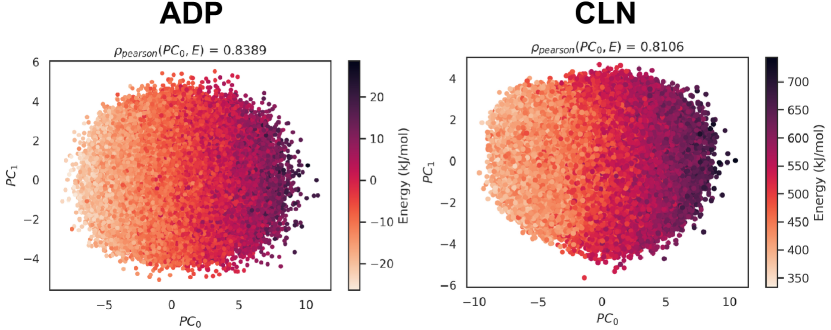
Figure 15: Projection of the full dimensional latent space embedding of all our (a) ADP and (b) CLN training data into the two leading principal components color-coded by the target atomistic configuration internal potential energy.

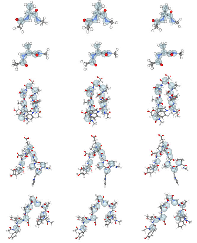
Figure 16: Atomic reconstructions generated from a fixed condition with different latent space instantiations. Each row represents a set of three atomic reconstructions for a fixed CG configuration. Faded blue spheres represent the input CG configuration overlaid on the atomic reconstruction. For ADP along the first three rows, the primary variation in these latent space samples are rotations of the methyl group hydrogens, as the rest of the peptide backbone and side chains are defined by the input CG configuration alone. For CLN along the final three rows, we notice the majority of configurational variation stems from side-chain motions along the C- and N-terminus.

After completing training for both our ADP and CLN models, we can visualize our latent space posterior $\mathbf{Z}$ by projecting our full-dimensional latent space into the first two Principal Components (PCs) of $\mathbf{Z}$ (Fig. 15 in the Supporting Information). Color-coding latent codes by the potential energy of the corresponding target configuration $U_{target}$ in each sample reveals a strong correlation between the leading PC and internal energy for both of our test systems ADP ($\rho_{\text{pearson}}(PC_{0}^{ADP},U_{target})\approx 0.84$) and CLN ($\rho_{\text{pearson}}(PC_{0}^{CLN},U_{target})\approx 0.81$). These strong correlation suggests our encoder effectively extracts features from the input data to encode physically meaningful features, reflected in the internal energy, of the target atomistic configuration within our latent space embedding. We can also interrogate the generative capabilities of our model by using our decoder to produce reconstructions of a fixed CG input under many different latent code instantiations (Fig. 16 in the Supporting Information). The diversity of valid generated structures which still adhere to the CG input suggest that the decoder is attentive to subtle variations in the latent code when reconstructing atomistic configurations. In all, these properties of our cVAE model and latent space embedding validate expected behavior: our encoder effectively distills information to the latent code from the input data, while our decoder purposes the latent code together with the condition to non-deterministically and generatively reconstruct atomistic structures.

2.5 Data curation

Our model learns to backmap a CG trajectory of a molecule by training on a reference atomistic trajectory of that molecule that we coarse-grain after the fact to yield exemplar pairs of atomistic and coarse grained frames (Fig. 1a). When backmapping to predict an atomistic structure ${\mathrm{AA}}^{t}$ we consider both the current CG structure ${\mathrm{CG}}^{t}$ along with the previous atomistic structure ${\mathrm{AA}}^{t-1}$. An important consideration when obtaining training data is the temporal spacing between consecutive frames ${\mathrm{AA}}^{t-1},{\mathrm{AA}}^{t}$, as it may be impossible to accurately recover molecular motions that occur faster than this time. We also find that it is critical to ensure the reference atomistic trajectory is sufficiently sampled and captures the relevant atomistic state transitions that are expected to be reflected in the backmapped atomisitic trajectory.

We train separate models on reference atomistic trajectories of alanine dipeptide (ADP) and the mini protein chignolin (CLN). Separate held-out trajectories for ADP and CLN are used as test sets for evaluating the performance of our model on in distribution data (Fig. 1b). As a more challenging generalization test of our method, we also backmap CG trajectories generated from a bespoke CG force-field, CGSchNet (Fig. 1c). We then evaluate structural, thermodynamic and kinetic statistics of our atomistic reconstructions against reference atomistic trajectories to evaluate performance of our method. In the following sections, we describe the details of the simulations methods used to generate the ADP and CLN trajectories we use to train and test our model.

2.5.1 Alanine dipeptide

Atomistic data

Atomistic trajectories of alanine dipeptide (ADP) used for training are collected by performing molecular dynamics simulations in explicit solvent using OpenMM ⁶³. We closely mimic the simulation procedures outlined Ref. ⁶⁴. Langevin dynamics simulations are performed with a 2 fs time-step in the NVE ensemble using the AMBER ff-99SB-ILDN force field ⁶⁵ within a cubic box containing 651 TIP3P water molecules randomly placed within a volume of (2.7273 nm)³. Electrostatics are treated using the particle-mesh Ewald (PME) method ⁶⁶ using a 1.0 nm cutoff for the direct space interactions. The length of all bonds involving hydrogen atoms are constrained. Steepest descent energy minimization is used to relax the initial system configuration to within an energy of 10 kJ/mol. We then assign initial velocities to the energy minimized configuration by sampling from a Maxwell-Boltzmann distribution at 300 K. A short 100 ps equilibration run is then performed followed by a 500 ns production run. This 500 ns production run comprises our training data. A separate 250 ns production run is performed to generate the in distribution data used for testing. In each case trajectory snapshots are saved every 1 ps, yielding 500,000 simulation frames for the training data and 250,000 simulation frames for the test data.

Coarse-grained data

For the CG representation of ADP, we choose to remove all solvent and represent the molecule using the five backbone carbon and nitrogen atoms (C, N, CA, C, N) and the carbon beta (CB) of the alanine residue, resulting in a total of six coarse grain atoms. A CG trajectory is generated from the above-mentioned all atom trajectory by slicing the coordinates to retain only the specified coarse grain atoms. The same coarse grain mapping is also applied to the all-atom forces to produce an associated set of instantaneous coarse grain forces. Using both the coarse grain coordinates and forces, bespoke CG force fields are recovered using CGSchNet ⁶⁷ neural network models. These ADP CG models are trained using the same data set from Refs.^{68, 67}, and are then used to generate out-of-sample data in the form of CG trajectories as a generalization test for our backmapping method to illustrate performance on real, noisy data. The trajectories used for backmapping consist of 100 separate simulations initalized at random configurations from the reference atomistic data set and containing a total of 4,000 frames each. Sequential CG simulation frames are temporally separated by the same 1 ps spacing as used in the training data trajectory. The training routines and hyperparameters of these CG force field models, as well as the simulation parameters for the out-of-sample CG simulations, are described in the Supporting Information.

2.5.2 Chignolin

Atomistic data

We use reference Chignolin (CLN) trajectories generated from atomistic simulations performed in Ref. ⁶⁸. Briefly recapping the protocols, these simulations are performed using the ACEMD program ⁶⁹ on GPUgrid ⁷⁰ at 350 K mimicking the setup originally used on the Anton supercomputer simulation ⁷¹. To sufficiently sample folding/unfolding transitions in CLN the data is produced through an MSM-based adaptive sampling strategy ⁷² consisting of an aggregated $\sim$187 $\mu$s of molecular dynamics simulation split into 3,744 short trajectories. Simulation snapshots are spaced by 100 ps culminating in a total of 1,868,861 frames. As each of the 3,744 trajectories are independent we simply split-off 3,650 for training and the remaining 94 for testing to comprise our in distribution test set.

Coarse-grained data

For a CG representation of CLN, we choose to remove all solvent and represent the molecule using just the 10 sequential $\alpha$-carbons (CA) atoms along the molecular backbone. Following the same procedure described above for ADP, a set of CG trajectories and associated forces are generated. The same CG coordinates and forces mapped from the atomistic data described in the preceding section are then used to train CGSchNet ⁶⁷ neural network force fields, which in turn are used to generate out-of-sample data for generalization tests of our backmapping model. We produce 1,000 separate trajectories containing 4,000 frames each and, similar to ADP, are initialized at random configurations from the reference atomistic dataset. In this case for CLN each frame is temporally separated by 1 ps, which differs from the 100 ps frame spacing in the training data. While we appreciate this frame spacing represents a different regime than our model is trained to operate in, the inherently accelerated nature of CG dynamics makes direct comparison between CG and atomistic time steps difficult. We appeal to a smaller frame spacing in this work to account for this inherent acceleration of CG dynamics and enable better sampling of short-lived, transient states within these trajectories. As with ADP, the training routines, model hyperparameters, and CG simulation parameters for the CLN coarse grain force fields are detailed in the Supporting Information.

3 Results

We present a data-driven and temporally coherent approach for backmapping coarse grained trajectories into full atomistic resolution. Our approach is based on training a conditional variational autoencoder (cVAE) to generate atomistic coordinates of a coarse grain (CG) configuration while also incorporating information from the previous atomistic configuration within the trajectory. The proposed method is applied to two biomolecular systems: alanine dipeptide (ADP) and the miniprotein Chignolin (CLN). The performance of our model is evaluated by measuring its ability to generate backmapped trajectories that preserve atomistic structural, thermodynamic and kinetic properties. Our model is trained on data consisting of pairs of atomistic and corresponding CG trajectories, that are obtained by mapping the atomistic data to CG resolution (Fig. 1a). For one evaluation test we apply our method to backmap CG trajectories generated from mapping separate held-out atomistic trajectories to CG resolution, which will be referred to as the in-distribution test set, or simply referred to as the test set (Fig. 1b). For a more challenging test of the generalization capabilities of our model, we apply our method to CG trajectories generated using a bespoke CG force-field CGSchNet ⁶⁷, which will be referred to as out-of distribution or generalization set (Fig. 1c). For both molecules ADP and CLN the in-distribution and generalization tests show excellent agreement in measures of structural, thermodynamic and kinetic similarity between our backmapped and atomistic trajectory data.

3.1 Alanine dipeptide

3.1.1 Energetics

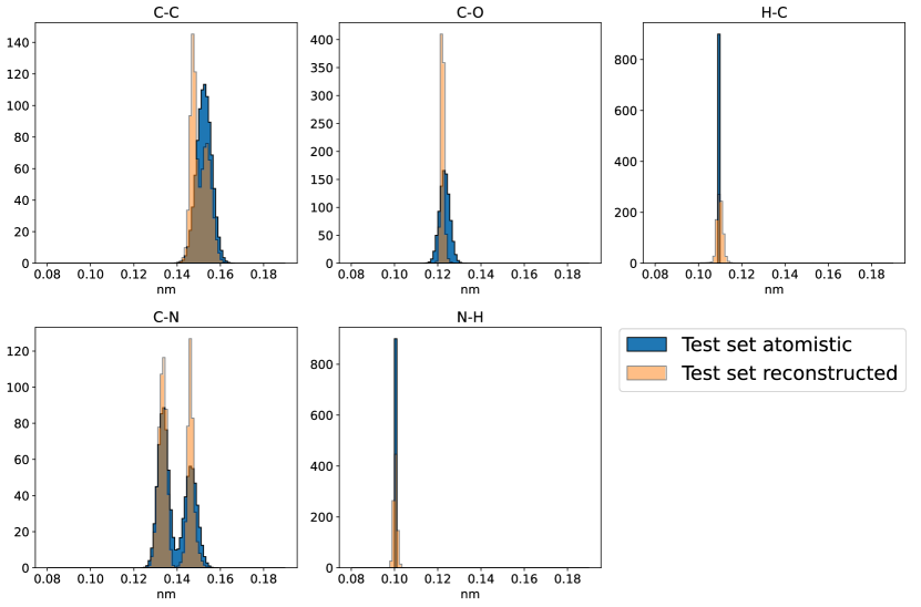
Figure 17: Bond length distributions delineated by element participation for the in distribution test set atomistic and backmapped trajectories for ADP.

As a first example, we apply our backmapping method to the small molecule alanine dipeptide (ADP) composed of 22 atoms from which we consider a coarse-graining into six CG beads along the peptide backbone. We evaluate structural similarity between atomistic and our backmapped trajectories by comparing distributions of the internal potential energy. The internal energy aggregates contributions from bonded and non-bonded interactions. As such, agreement between atomistic and reconstructed energy distributions serves as a good indicator of overall structural similarity. The energy distribution for the in distribution test set shown in Fig. 3a reveals that our model nearly identically reproduces the energy distribution of the original atomistic data. Similarly, the energy distribution for the generalization test set obtained by backmapping a trajectory generated with CGSchNet ⁶⁷ is displayed in Fig. 3b. This out-of distribution test represents a more difficult exercise for our model, as it must generalize to real CG simulated data generated by a different, approximate force field than our model was not exposed to during training. Our model yields backmapped structures that nearly identically match the energetics of the atomistic reference data. The only noticeable deviation for both test sets are small high-energy tails of the backmapped reconstructions (Fig. 3). While these rare high-energy configurations can be attributed to minor deviations in a few bond length and angle distributions, we find overall excellent agreement between distributions of local intramolecular features between backmapped and reference structures (Fig. 17-20 in the Supporting Information). Our backmapping method in general reconstructs atomistic ADP trajectories with high structural and energetic similarity to reference atomistic data while also generalizing well to unseen and real CG force fields, and as a result generates visually identical backmaped structures (Fig. 4e and Fig. 16 in the Supporting Information).

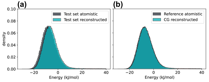
Figure 3: Comparison of the internal potential energy distributions for atomistic and backmapped ADP trajectories. (a) Internal energies for the held out test set trajectory and the atomistic reconstructed trajectory generated by backmapping a manual coarse graining of the original atomistic trajectory. (b) Generalization test comparing reference atomistic trajectories obtained from Ref. ⁷³ to our model-generated backmappings of a real CG simulation conducted using CGSchNet ⁶⁷.

3.1.2 Thermodynamics

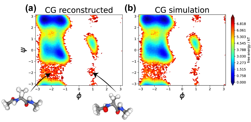
Figure 21: Comparison of MSM-reweighed ADP FES between the (a) the backmapped CG reconstructed trajectory and (b) the original CG simulation performed with CGSchNet. Insets show a superposition of seven configurations within the transition paths between select meta-stable states. Although these configurations are rarely seen in the atomistic training data, our model effectively generalizes to reliably reconstruct these high-energy configurations from the data simulated with CG force fields.

We evaluate thermodynamic similarity by comparing free energy surfaces (FES) of our reconstructed trajectories to reference atomistic data. We construct our FES in the space of the backbone dihedral angles $(\phi,\psi)$ as they have proven to be good collective variables for characterizing the conformational states of ADP ^{74, 75}. In Fig. 4a we present the FES in $(\phi,\psi)$ for the in distribution test set atomistic trajectory compared to the CG backmapped trajectory FES in Fig. 4b. Our atomistic reconstruction here reproduces a nearly identical FES to the ground truth atomisitic data demonstrating that for in distribution data our model accurately captures the ground truth thermodynamics. For the generalization test we also present a FES generated from a reference atomistic trajectory (Fig. 4c) compared to the FES of a CG backmapped trajectory generated from a CG simulation performed with CGSchNet ⁶⁷ (Fig. 4d). Once again our reconstruction is in excellent agreement with the atomistic reference, importantly correctly identifying the five major meta-stable states of ADP. In Fig. 4e we show a superimposed collection of configurations for each of these meta-stable states from the reference, test set reconstructed and CG reconstructed trajectories. For both in distribution and out of distribution data our model reconstructs visually identical configurations with remarkable similarity to the atomistic reference data. Note that the CG model yields configurations throughout the transition paths between meta-stable states, for example ($\phi\approx-2$,$\psi\approx-2$). While those configurations are underrepresented in the atomistic trajectory due to high-energy barriers, the smoothed energy landscape of the CG force field enables broader and more frequent exploration of these regions of phase space. We find our model generalizes well to those sparsely sampled areas and accordingly reconstructs these high-energy configurations (Fig. 21 in the Supporting Information). Overall, our backmapping scheme reproduces the FES for ADP that are in excellent thermodynamic agreement with reference atomistic data for both our in distribution and generalization tests.

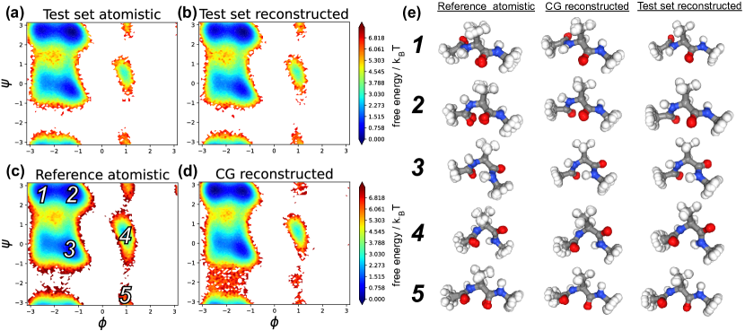
Figure 4: Comparison of atomistic and backmapped MSM-reweighted Free Energy Surfaces (FES) for ADP. Ramanchandran plots for the in distribution test set that includes (a) a held-out atomistic trajectory and (b) our model generated backmapping of the manually coarse grained atomistic trajectory. For a more challenging test of generalizability we compare the Ramachandran plots for (c) a reference atomistic trajectory taken from Ref. ⁷³ and (d) a backmapping of a CG simulation performed using CGSchNet ⁶⁷. Labeled in (c) are phase space locations for the five meta-stable states of ADP. (e) Seven superimposed configurations near each of these five major meta-stable states from (c) the reference atomistic, (d) the CG reconstructed and (b) the test set reconstructed trajectories.

3.1.3 Kinetics

An important aspect of the proposed method is the incorporation of the previous trajectory configuration as a conditional input for our ML model. This provides temporal information required to achieve temporal coherence between consecutive frames, which is typically omitted in traditional backmapping strategies. Here, we test the temporal coherence of our backmapped trajectories by analyzing kinetics in terms of implied process timescales and velocity distributions.

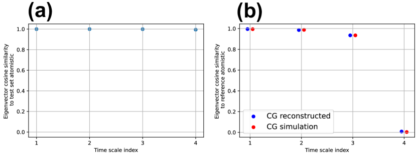
Figure 22: Cosine similarity between recovered MSM eigenvectors of atomistic and backmapped ADP trajectories. (a) The in distribution test set cosine similarity between atomistic and backmapped trajectories. (b) Cosine similarity between MSM eigenvectors of the backmapped data and the original CG data with respect to the reference atomistic data.

We compare kinetic agreement between ground truth atomistic data and our backmapped reconstructions by building Markov State Models (MSMs) ^{76, 77, 78, 79, 80} to characterize and compare the recovered physical processes and timescales. Construction and estimation of MSMs are carried out using the Deeptime ⁸⁰ software library. We construct MSMs in $\phi$,$\psi$ space for ADP and perform state assignment by discretizing the phase space with 100 k-means centroids fit onto the atomistic data. These same 100 centroids are then also used to generate state assignments for the backmapped trajectory to which we compare. Complete validation of the MSM with associated clustering plots and implied timescale analysis for lag time selection is provided in the Supporting Information. Shown in Fig. 5a are the recovered timescales for the test set atomistic and test set backmapped data. Our backmapped trajectory reproduces the atomistic timescales within error for all recoverable processes. A result of using the same state assignments when building the original atomistic and backmapped MSMs is that the elements of the recovered eigenvectors characterize eigenfluxes between the same states. We can therefore measure the cosine similarity between these eigenvectors to quantitatively validate that these timescales correspond to the same physical processes between the original atomistic and the backmapped trajectories. Indeed, shown in Fig. 22a in the Supporting Information we confirm via this cosine similarity measure that the MSM eigenvectors are effectively identically recovered for the backmapped trajectory of in distribution test set.

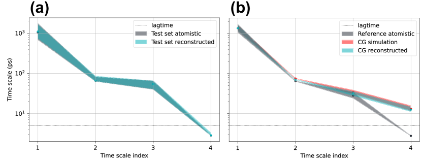
Figure 5: Implied timescales of atomistic and backmapped CG trajectories for ADP. (a) Comparisonon of timescales recovered for the test set atomistic and test set reconstructed trajectories. (b) Implied timescales calculated for the reference atomistic data taken from Ref. ⁷³ compared to the backmapped CG simulation performed with CGSchNet ⁶⁷ along with the original CG simulation. Timescales for the backampped and CG simulated data are normalized such that the dominant processes is the same as the reference atomistic trajectory. Errors are estimated with Bayesian sampling and represent a $95\%$ confidence interval of the timescales of the sampled MSMs.

Shown in Fig. 5b is a comparison of the implied timescales between reference atomistic data, backmapped trajectories generated by our model and the original CGSchNet CG simulation. For both the CG backmapped data and the original CG simulation we normalize the implied timescales such that the dominant (slowest) process matches the reference atomistic data. We perform such a normalization to correct for the fact that CG models typically sample configurational landscapes at an accelerated rate compared to atomistic force fields due to absence of explicit solvent and elimination of atomistic degrees of freedom that can cause the coarse-grained degrees of freedom to be accelerated by different scaling factors ^{18, 19, 81, 20, 21}. This normalization also serves as a visual convenience when comparing deviations of timescales between the accelerated CG dynamics and the atomistic data. An alternative method to this rescaling approach that provides the same information would simply measure timescale ratios instead. We report once again overall excellent agreement of the implied timescales, within error, between our backmapped and reference atomistic trajectories in Fig. 5b, with the exception of the fourth, and subsequent, timescales that are faster than our lag time of 5 ps and therefore below the resolution limit of our MSM. We also validate again in Fig. 22b in the Supporting Information by comparing MSM eigenvector similarity that these first three timescales indeed correspond to the same physical processes between these two data sets. The backmapped CG simulated data ultimately reflects the kinetics produced by the coarse-grained model, evidenced by the nearly identical timescales of the CG simulation and backmapping in Fig. 5b. Nevertheless, upon normalization of the timescales our excellent agreement for these generalization results suggesting the ratio of timescales between processes is preserved upon backmapping with our model.

A result of conditioning our backmappings using previous atomistic configurations we find our model is capable of successfully generating backmapped trajectories that reproduce intra-frame root mean square velocity distributions (Fig. 6). The distribution of velocities is an effective measure of the deviation of atomic coordinates between consecutive frames. Although our model is not explicitly trained to match intra-frame velocities, the temporal coherence built into our network architecture and training procedure enables the trained network to accurately reproduce these velocity distributions. The excellent agreement we observe for the in distribution data is enabled by the known and directly comparable spacing between frames. The temporal spacing between consecutive frames for the in distribution test set is well-defined by the frame spacing of the atomistic reference simulation, i.e., 1 ps. However, the specific temporal spacing is more obscure for the generalization set, as a direct consequence of the CG dynamics. While most CG models target thermodynamic consistency with a yet higher resolution model or experimentally observed properties, kinetic consistency is typically neglected. In general, CG force fields effectively accelerate simulation dynamics as a consequence of smoothing the energy landscape and lowering energy barriers. However, the timescales for transitions between meta-stable states are typically not rescaled uniformly ^{18, 19, 81, 20, 21}. To account for this inherent acceleration due to CG force fields, we rescale the velocity distribution of the backmapped generalization set data by a constant factor such that the mean of the velocity distribution matches the mean of the velocity distribution for the test set atomistic data. Applying this empirical correction we see reasonable agreement in the shape of the velocity distributions between the backmapped generalization set data and the native atomistic data, suggesting for ADP here our backmapping model is capable of reconstructing realistic atomic velocities up to a constant scaling factor for data originating from CG force fields.

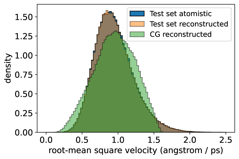
Figure 6: Comparison of atomistic and backmapped root mean square velocity distributions for ADP. Velocities are calculated atom-wise between sequential frames using a finite forward difference method and aggregated into a distribution over all atomic velocities. Velocities for the CG reconstructed data corresponding to the generalization set are rescaled by a constant factor ($\sim$3.25) such that the mean of the CG reconstructed velocities matches the mean of the test set atomistic velocities.

3.2 Chignolin

3.2.1 Energetics

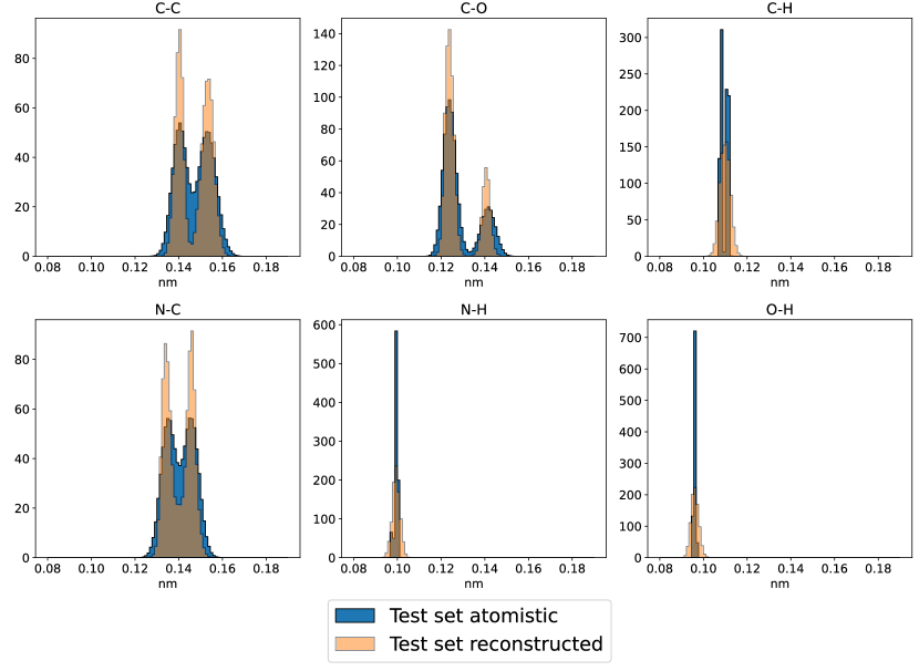
Figure 33: Bond length distributions delineated by element participation for the in distribution test set atomistic and backmapped trajectories for CLN.

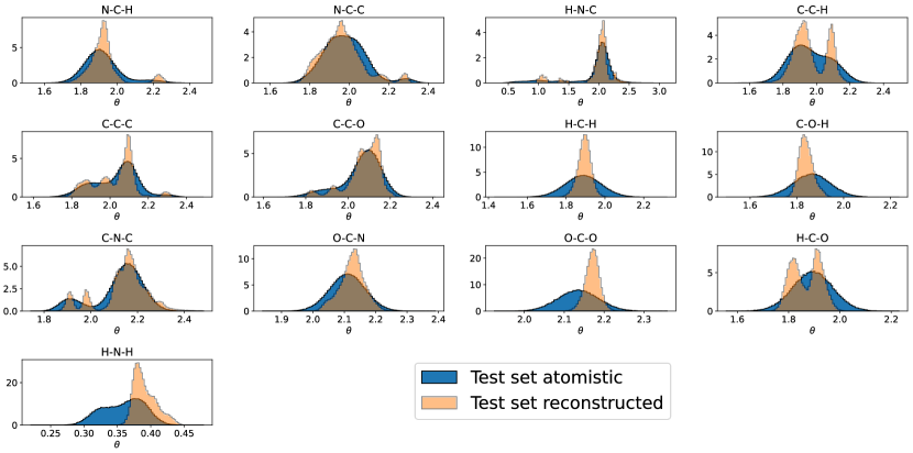
Figure 34: Atomic angle distributions delineated by element participation for the in distribution test set atomistic and backmapped trajectories for CLN.

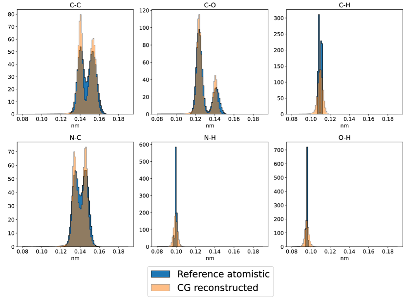
Figure 35: Bond length distributions delineated by element participation for the generalization test reference atomistic and backmapped CGSchNet trajectories for CLN.

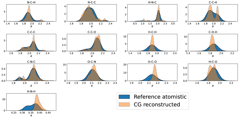
Figure 36: Atomic angle distributions delineated by element participation for the generalization test reference atomistic and backmapped CGSchNet trajectories for CLN.

The second molecular system we apply our backmapping method to is the miniprotin Chignolin (CLN), which is composed of 10 residues with 175 atoms from which we consider a coarse graining into the 10 $\alpha$-carbons along the peptide backbone. Compared to ADP, the scale and complexity of CLN presents a more challenging test case for both our backmapping and accurate CG force field construction. We once again compare distributions of the internal energy as an indicator for structural similarity between reference atomistic and our backmapped data. Shown in Fig. 7a is a comparison of the internal energies for the in distribution test set atomistic and backmapped trajectories, while a comparison for the generalization set data is presented in Fig. 7b. These results show excellent energetic overlap between the reference atomistic and our backmapped data for both the in distribution and generalization sets. The internal energies recovered from the backmapped CGSchNet simulation in Fig. 7b from the generalization test show longer high-energy tails compared to the in distribution test in Fig. 7a. The origins of these higher-energy reconstructed configurations can be explained by an examination of the bond lengths and angles revealing the presence of very slightly contracted bond length distributions in the generalization set compared to the in distribution test set (Figs. 33-36 in the Supporting Information). Our backmapped trajectories nevertheless show overall excellent agreement in these local intermolecular features and energetics, and therefore also produce visually convincing atomistic reconstructions (Fig. 8e and Fig. 16 in the Supporting Information).

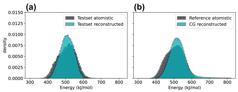
Figure 7: Potential energy distributions of atomistic and backmapped CLN trajectories for (a) the in distribution test set and (b) the generalization set.

3.2.2 Thermodynamics

We construct Free Energy Surfaces (FES) using the basis recovered from Time-lagged Independent Component Analysis (TICA) ^{82, 74, 83, 84} to compare thermodynamic similarity between reference atomistic data and our backmapped trajectories. Unlike ADP, there are no simple intuitive variables capable of compactly representing the CLN FES, so we instead use TICA as a dimensionality reduction technique to extract a low-dimensional representation for the CLN phase space. Using our entire reference atomistic dataset we first learn a TICA embedding into the first two non-trivial Independent Components (ICs) using all 45 pairwise $\alpha$-carbon distances as features ^{68, 67, 85, 86}. This learned TICA model provides us with a fixed basis set we use for constructing an FES in these two leading ICs for the atomistic and backmapped data from both our in distribution and generalization data sets.

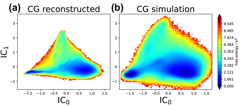
Figure 37: Comparison of MSM-reweighed FES for CLLN along the first two Independent Components (ICs) of a TICA model fit to the reference atomistic dataset between the (a) the backmapped CG reconstructed trajectory and (b) the original CG simulation performed with CGSchNet.

Shown in Fig. 8 is a comparison of these CLN FESs for in distribution test set atomistic (Fig. 8a) and backmapped (Fig. 8b) trajectories, alongside the generalization set reference atomistic FES (Fig. 8c) and the FES obtained from backmapping a CG simulation performed with CGSchNet ⁶⁷ (Fig. 8d). In each case the backmapped FES recovers the presence of the three primary meta-stable states in CLN and produces visually identical atomic reconstructions compared to the atomistic reference (Fig. 8e). We notice our backmapped FES are contracted near regions corresponding to the folded state (labeled 1) and the misfolded state (labeled 2) compared to the unfolded ensemble (labeled 3). Correspondingly, backmapped structures extracted from the folded and misfolded states display slightly less configurational variability compared to atomistic reference than structures visualized from the unfolded ensemble (Fig. 8e). We suspect this is due to a loss-conserving strategy by the network: comparatively less loss is sacrificed by predicting a (nearly) fixed configuration for CG structures corresponding to folded and misfolded states compared to the benefit of capturing the diversity of possible structures in the unfolded ensemble. This results in more comprehensive coverage of the unfolded ensemble in our backmapped data compared to the folded and misfolded states. We also notice that the misfolded state is noticeably less stable in the generalization set backmapping (Fig. 8d) compared to the reference atomistic data (Fig. 8c). Indeed, we find this property to be a reflection of the misfolded state being inherently less stable in the original CG simulation as well (Fig. 37 in the Supporting Information). While our backmapping method does a reasonable job of reproducing the atomistic FES, we find that are ultimately limited by the underlying accuracy of the CG simulation that we backmap.

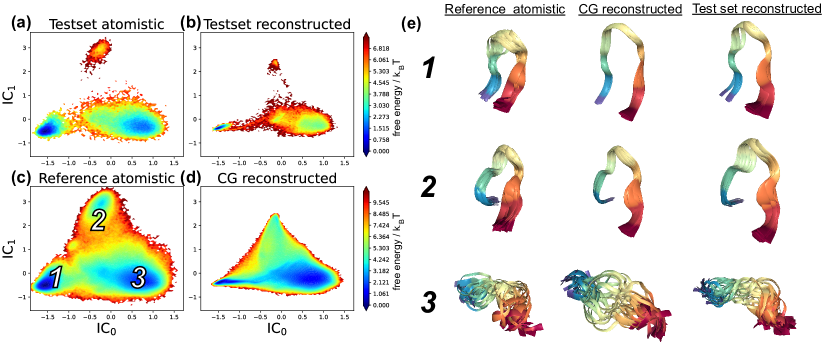
Figure 8: Comparison of the atomistic and backmapped MSM-reweighted Free Energy Surface (FES) for CLN. The FES for CLN is represented in the basis of the two leading non-trivial Independent Components (ICs) of a Time-lagged Independent Component Analysis (TICA) model fit to the reference atomic dataset. Shown are FES of the in distribution test set atomistic (a) and backmapped (b) trajectories, alongside the reference atomistic data (c) and the corresponding backmapped CGSchNet simulation (d) from the generalization set. (e) Visualization for a collection of 25 superposed structures from the three meta-stable states taken from the reference atomistic data (c), the backmapped CG reconstructed data (d) and backmapped in distribution test set trajectory (b).

3.2.3 Kinetics

We evaluate kinetic similarity between reference atomistic data and our backmapped trajectories by comparing similarity of MSM-recovered implied timescales and processes. We perform state space discretization for our MSMs within the same two-dimensional TICA basis used to construct our FES. Data from the reference atomistic trajectories in this two-dimensional TICA space is fit to determine 150 k-means centroids identifying the state space decomposition. We then use these same 150 centroids to generate state assignments when building separate MSMs for other atomistic and backmapped data within the in distribution and generalization data sets. Using the same TICA projection and set of cluster centers between MSMs ensures direct comparability of the recovered eigenvectors and allows us to determine similarity of the recovered processes. We use the same methodology as with ADP here for CLN for quantifying similarity of processes by measuring the cosine similarity of the MSM eigenvectors. In the cases where not all 150 states are utilized, we construct MSMs using only occupied states and compute cosine similarity using only this subset of mutually occupied states between the two MSMs being compared. Using this approach we can quantitatively ensure the that implied timescales in fact correspond to the same physical processes between the two data sets. As with ADP, complete details on MSM construction and validation are provided in the Supporting Information.

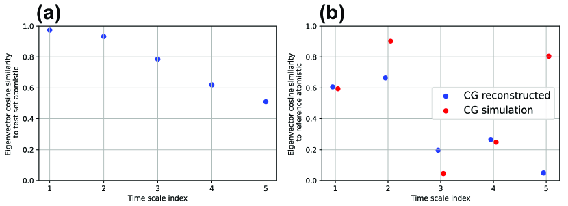
Figure 38: Cosine similarity between recovered MSM eigenvectors of atomistic and backmapped CLN trajectories. (a) The in distribution test set cosine similarity between atomistic and backmapped trajectories. (b) Cosine similarity between MSM eigenvectors of the backmapped data and the original CG data with respect to the reference atomistic data.

Presented in Fig. 9a is a comparison of implied timescales between atomistic and backmapped trajectories for the in distribution test set. For the in distribution test set our backmapped reconstruction precisely reproduces within error all implied timescales. The large gap between the 2${}^{\text{nd}}$ and 3${}^{\text{rd}}$ timescales suggests the majority kinetic variance is captured in the first two processes, which we recover with >90% cosine similarity, and for the final remaining processes greater than our lag time – and therefore the only other resolvable process by our MSM – we also recover with $\sim$80% cosine similarity (Fig. 38a in the Supporting Information). Comparison of implied timescales for the generalization set between the reference atomistic data, backmapped CGSchNet ⁶⁷ simulation and the original CG simulation is shown in Fig. 9b. We follow the same approach here as with ADP, where we normalize the implied timescales for data generated from CG simulations by a constant factor such that their slowest timescale matches the slowest timescale from the reference atomistic data. This normalization accounts for the inherently accelerated dynamics of CG simulations and enables us to effectively compare the ratio of implied timescales ^{18, 19, 81, 20, 21}. The ratio between the first two timescales is poorly recovered for both the backmapped data and the original CG simulation compared to the reference atomistic data. Comparison of the cosine similarity between these processes reveals the 1${}^{\text{st}}$ processes is recovered with $\sim$60% similarity for both the backmapped data and the CG simulation, while the 2${}^{\text{nd}}$ processes is recovered with also $\sim$66% similarity for the backmapped data and $\sim$90% similarity for the original CG simulation (Fig. 38b in the Supporting Information). While the ratio in the timescales for the faster 3${}^{\text{rd}}$ and 4${}^{\text{th}}$ processes seems to be better conserved in the original CG simulation, our backmapped data actually recovers these processes with slightly better similarity than the original CG simulation (Fig. 38b in the Supporting Information). The fact that our method precisely recovers kinetics for the in distribution data but can only approximately recovers kinetics when backmapping real CG simulated data confirms that our method produces backmapped trajectory data that is largely a reflection of the kinetics expressed in the underlying CG data.

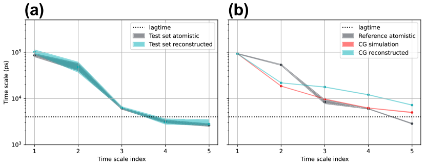
Figure 9: Implied timescales of atomistic and backmapped CG trajectories for CLN. (a) Comparison of implied timescales from atomistic and backmapped trajectories for the in distribution test set. (b) Implied timescales for the reference atomistic data, the original CGSchNet simulation and the backmapped CGSchNet simulation. Timescales for the original CG simulation and backmapped data are normalized such that the dominant (slowest) processes matches the slowest reference atomistic timescale.

Lastly, we compare velocity distributions as an indicator of temporal coherence between sequential frames in our backmapped reconstructions. Shown in Fig. 10 is a comparison of frame-by-frame root mean square velocity distributions for the reference and backmapped in distribution test set data alongside the backmapped CGSchNet simulation data. For the in distribution test set the velocities are an excellent match between the reference and backmapped data. Mimicking our approach with ADP, to account for the inherently accelerated dynamics of the CGSchNet force field we use a constant factor to rescale the atomic velocities such that the mean of the backmapped generalization set velocities matches the mean of the test set atomistic velocities. After applying this constant scaling we notice excellent agreement in the shape of the velocity distributions between the backmapped generalization set data and the original atomistic data. We note that the scaling factor used to correct the CLN velocities ($\sim$17.81) is much larger than the scaling factor used for the ADP velocities ($\sim$3.25), suggesting a more substantial acceleration of backmapped CLN dynamics due to the CG force field compared to ADP. This relative speed-up of the backmapped CLN CG simulation could be attributed to the more severe coarse-graining of CLN from 175 atoms to 10 beads (17.5$\times$ reduction) compared to the ADP model from 22 atoms to 6 beads ($\sim$3.67$\times$ reduction). This more dramatic reduction in the degrees of freedom upon coarse-graining for the CLN model could result in the CLN CG simulation operating in a comparatively ’smoother’ free energy surface than ADP, and therefore leading to the relatively faster atomic motions identified by the velocity distributions.

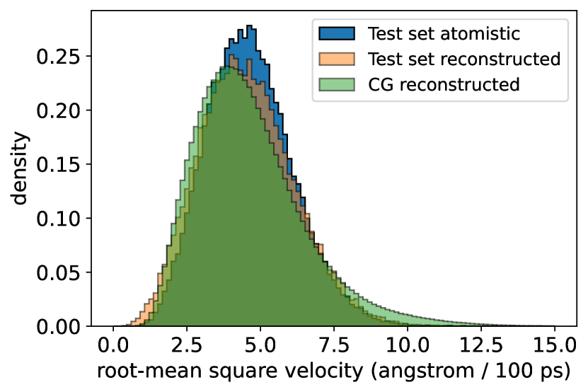
Figure 10: Comparison of atomistic and backmapped root mean square velocity distributions for CLN. Velocities are calculated frame-by-frame using a finite forward difference method and represented in angstrom / 100 ps, as 100 ps is the native temporal spacing between frames in the reference atomistic data ⁶⁸. The backmapped generalization set velocities are rescaled by a constant factor ($\sim$17.81) such that the mean of the CG reconstructed velocities equals the mean of the test set atomistic velocities.

4 Conclusions

We present in this work a data-driven and temporally coherent scheme for backmapping CG trajectories into atomistic resolution. Our approach trains a conditional variational autoencoder (cVAE) to reconstruct atomistic detail given the target CG configuration and the previous atomistic structure. Our method is showcased here to backmap two popular biomolecular systems: alanine dipeptide (ADP) and the miniprotein chignolin (CLN). We train our model using a reference atomistic trajectory which we coarse-grain post hoc to produce exemplar pairs of atomistic and CG configurations (Fig. 1a). We test that our backmapping method on both in distribution data generated from backmapping a CG trajectory produced by coarse-graining held-out atomistic data (Fig. 1b), and out of distribution data generated from a real CG simulation performed using CGSchNet ⁶⁷. We evaluate the performance of our model in terms of capability to reproduce structural, thermodynamic and kinetic properties of reference atomistic systems. To this end, structural similarity is probed by comparing distributions of potential energies and local structural features, such as bond lengths and angles. Thermodynamic similarity is tested by analyzing free energy surfaces that are constructed in terms of collective variables. Kinetic agreement is tested by comparing implied timescales of processes identified by MSMs, while temporal coherence between consecutive frames is analyzed in terms of intra-frame velocity distributions. Our model yields backmapped trajectories for the in distribution test set that are in good agreement with atomistic data. Moreover, our model generalizes well producing convincing atomic reconstructions for out of distribution data obtained from CGSchNet simulations. While we notice slightly better generalizability to CGSchNet simulations of ADP compared to the more complex CLN molecule, we find our method generates backmapped trajectories that largely maintain thermodynamic and kinetic properties reflected in the original CG simulation while also reconstructing atomistic velocities up to a constant scaling factor. Errors in our backmapped reconstructions on the out of distribution generalization data can be attributed to both the performance and expressivity of our backmapping cVAE model compounded with biases and inaccuracies of the CGSchNet force field used to generate the CG trajectories. In the case of ADP, the highly accurate CGSchNet model leads to overall good backmapping generalization performance. For CLN, the CGSchNet model is comparatively lower-fidelity which we find results in slightly poorer generalization by our backmapping model in comparison to ADP. Ultimately, the backmapping scheme presented in this work can serve as a tool to analyze thermodynamic and kinetic properties of a CG system at atomistic resolution while also generating temporally coherent backmapped trajectories.

Future work will strive to improve upon the data efficiency and training/inference routines of our method. The backbone of our model primarily uses convolutional neutral networks (CNNs) operating on voxelized representations that are converted to and from Cartesian coordinates. While CNNs offer excellent expressibility via naturally hierarchical processing, they are not rotationally covariant and therefore require that we train our network with random rigid rotations to implicitly learn sensitivity to arbitrary alignments. Using explicitly covariant network architectures ^{87, 88, 89}, such as those employed in the backmapping scheme by Wang et al. ⁴³, can lead to superior data efficiencies without the need to train with random rotations. Training routines could also be augmented to incorporate more inductive biases that may benefit backmapping, such as: (i) better emphasizing sparsely populated regions of configurational space, which could be accomplished by accompanying training samples with thermodynamic or dynamical path weights; (ii) an autoregressive training protocol could be employed to improve the temporal coherence by using a recurrent approach to predict multiple consecutive frames each forward pass; (iii) further encourage the model to utilize knowledge of preceding trajectory frames by augmenting the training loss to incorporate information that is explicitly based on velocities or higher order time derivatives.

Data Availability

A complete PyTorch implementation of our model with associated training routines, data, and pretrained model weights for ADP and CLN along with Jupyter Notebooks demonstrating the energetic, thermodynamic, and kinetic analyses performed in this work is provided via the Materials Data Facility (MDF) ^{90, 91} at DOI:10.18126/tf0h-w0jz ⁵².

Supporting Information

4.1 cVAE architectural details and training settings

We discuss here details and hyperparameters in our cVAE architecture and training setup, with all code and datasets publicly available at DOI:10.18126/tf0h-w0jz ⁵². Typical VAEs are composed of an encoder-decoder architecture where the encoder process an input into a fixed dimensional latent code that the decoder purposes to generate reconstructions of the input. Conditional VAEs (cVAEs) differ from this paradigm by defining an auxiliary conditional variable alongside the reconstruction target, which is passed to the decoder alongside the latent code when generating reconstructions. This cVAE framework enables the decoder alone to act as a generative model provided a conditional variable as input and a randomly sampled latent code as a source of generative noise.

In our application, we strive to produce temporally coherent backmappings by incorporating as input previous atomistic configurations ${\mathrm{AA}}^{t-1}$ alongside the current coarse grain ${\mathrm{CG}}^{t}$ configuration when generating reconstructions $\hat{{\mathrm{AA}}^{t}}$. This temporal coherence is achieved in our cVAE framework by defining the reconstruction target $\mathbf{y}={\mathrm{AA}}^{t}$ and the conditional variable as the tuple of configurations $\mathbf{c}=({\mathrm{CG}}^{t},{\mathrm{AA}}^{t-1})$.

Our model operates on 3D spatially voxelized particle densities delineated for each particle which we can readily transform to/from Cartesian coordinates (cf. Sec. 2.1 of the main text). Presented in Fig. 11 is an illustration of our cVAE architecture and data flow exemplified for the alanine dipeptide (ADP) molecule. Beginning in the top left of Fig. 11, the input to our encoder $\mathbf{x}$ are the three configurations (${\mathrm{AA}}^{t-1}$, ${\mathrm{CG}}^{t}$, ${\mathrm{AA}}^{t-1}$) voxelized and concatenated along their particle dimension $\mathbf{x}=[{\mathrm{VOX}}^{{\mathrm{AA}}^{t-1}}||{\mathrm{VOX}}^{{\mathrm{CG}}^{t}}||{\mathrm{VOX}}^{{\mathrm{AA}}^{t-1}}]\in\mathbb{R}^{d\times d\times d\times(2N+n)}$, where $d$ is the number of grid points used for the spatial discretization, $N$ is the number of atoms within each atomistic configuration and $n$ is the number of beads within each CG configuration. For this exemplar case of ADP shown here we use a spatial discretization of $d=12$ with $N=22$ and $n=6$, yielding an input tensor with dimensionality $\mathbf{x}\in\mathbb{R}^{12\times 12\times 12\times 50}$. The different components of the input tensor are color-coded to designate the configurations associated with the conditional variable (${\mathrm{CG}}^{t}$, ${\mathrm{AA}}^{t-1}$) (light blue) and the reconstruction target ${\mathrm{AA}}^{t}$ (orange).

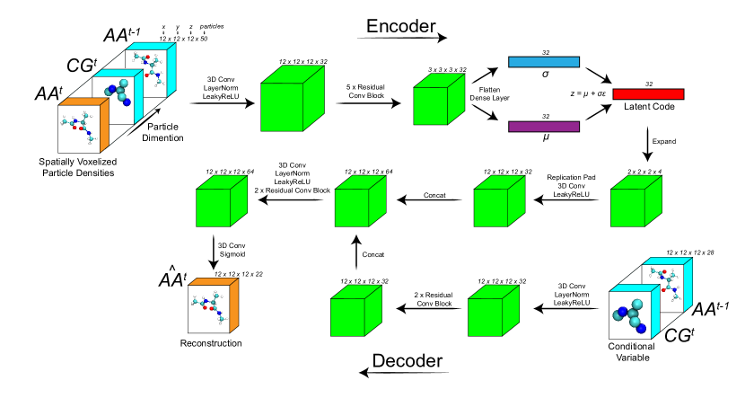
Figure 11: Schematic illustration of our cVAE architecture and data flow exemplified with particle dimensions above each tensor corresponding to our model trained on ADP.

The encoder processes the input $\mathbf{x}$ using a series of (residual) CNN modules. Each arrow in Fig. 11 represents a series of operations performed on a representation with the resultant tensor dimensionality shown above the subsequent block. For example, the first arrow in the top left of Fig. 11 indicates a series of computations on the input $\mathbf{x}$ involving a 3D convolution, followed by a LayerNorm and lastly a LeakyReLU activation yielding an intermediate representation with dimension $12\times 12\times 12\times 32$. Here, $d_{hidden}=32$ represents the hidden channel dimensionality of the network. The next step within the encoder involves sequential application of a 5$\times$ series of residual convolutional blocks. In some cases we use different hidden channel dimensions for the encoder $d_{hidden}^{Encoder}$ and the decoder $d_{hidden}^{Decoder}$. A schematic illustration of our residual convolution block is shown in Fig. 12. In the case where the dimensionality of the input changes within the residual convolutional block, instead of a simple identity operation the residual is accommodated to the appropriate dimensionality using max pooling and 1x1 3D convolutions. A variety of strides and kernel sizes are used within the five sequential residual convolutional blocks of the encoder to yield a representation with dimensionality $3\times 3\times 3\times 32$. This representation is then flattened into a $3\times 3\times 3\times 32=864$-dimension vector which is processed with two separate dense layers to yield two $32$-dimensional representations corresponding to the mean $\boldsymbol{\mu}$ and standard deviation $\boldsymbol{\sigma}$ of the cVAE latent space. At training time, the latent code $\mathbf{z}$ is then sampled from $\boldsymbol{\mu}$ and $\boldsymbol{\sigma}$ using the reparamterization trick $\mathbf{z}=\boldsymbol{\mu}+\boldsymbol{\epsilon}\odot\boldsymbol{\sigma}$ where $\boldsymbol{\epsilon}$ is sampled from an isotropic Gaussian $\boldsymbol{\epsilon}\sim\mathcal{N}(\mathbf{0},\mathbf{I})$. Here, the dimension of the latent space is $d_{latent}=32$ such that $\mathbf{z}\in\mathbb{R}^{d_{latent}=32}$.

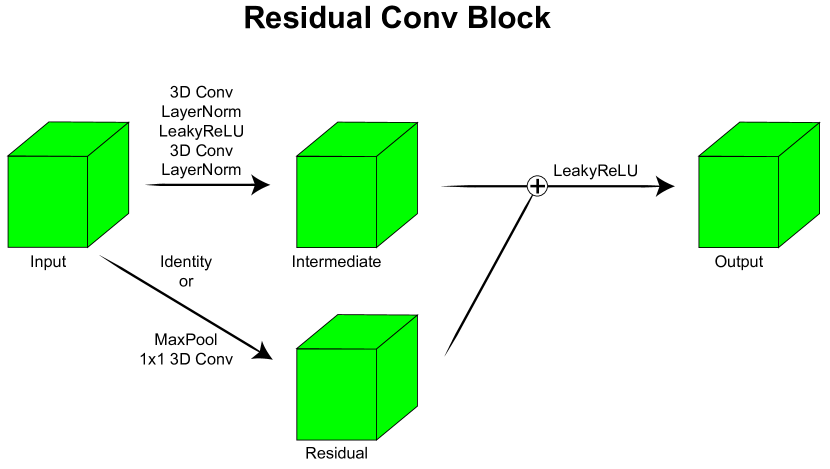
Figure 12: Schematic illustration of residual convolutional block used within our cVAE architecture.

Following extraction of the latent code $\mathbf{z}$ from the encoder, the decoder is passed the latent code $\mathbf{z}$ together with the conditional variable $\mathbf{c}=[{\mathrm{VOX}}^{{\mathrm{CG}}^{t}}||{\mathrm{VOX}}^{{\mathrm{AA}}^{t}}]$ to generate the voxelized reconstruction ${\mathrm{VOX}}^{\hat{{\mathrm{AA}}}^{t}}$. We can ultimately transform this output voxelized representation ${\mathrm{VOX}}^{\hat{{\mathrm{AA}}}^{t}}$ into Cartesian coordinates $\hat{{\mathrm{AA}}}^{t}$ for downstream application using the methods outlined in Sec. 2.1 of the main text. The decoder begins with separately processing $\mathbf{z}$ and $\mathbf{c}$, which are later concatenated and further processed to yield the target reconstruction. First, displayed in the bottom right of Fig. 11 the conditional variable $\mathbf{c}$ of dimension $12\times 12\times 12\times 28$ (there are 28=22+6 particle channels for $\mathbf{c}$ due to the 22 atoms within the atomistic structure the 6 beads of the coarse grain structure) is processed using (residual) 3D convolutions into an intermediate $12\times 12\times 12\times 32$-dimensional representation. Concurrently, the $d_{latent}=32$-dimensional latent code $\mathbf{z}$ is reshaped into a 4D tensor of shape $2\times 2\times 2\times 4$. This representation is then expanded using the PyTorch replication padding and processed with 3D convolutions to generate a compatible $12\times 12\times 12\times 32$-dimensional intermediate representation of the latent code. The processed conditional variable and latent code are then concatenated along the final dimensional to yield a $12\times 12\times 12\times 64$-dimensional representation, which we further process with (residual) convolutions to yield the $12\times 12\times 12\times 22$-dimensional output. The final particle-dimension of this output tensor ${\mathrm{VOX}}^{\hat{{\mathrm{AA}}}^{t}}$ corresponds to the number of particles in the target atomistic configuration. A terminal sigmoid activation scales the voxel values between 0-1 and we interpret each channel as a voxelized particle density, which we can ultimately then collapse back into Cartesian coordinates $\hat{{\mathrm{AA}}}^{t}$ as the complete atomistic reconstruction.

The training loss for our model described in detail in Sec. 2.3 of the main text is

$$\mathcal{L}=\mathcal{L}_{{\mathrm{VOX}}}+\mathcal{L}_{{\mathrm{AA}}}+\mathcal{L}_{\text{CG}}+\mathcal{L}_{\text{EDM}}+\lambda\mathcal{L}_{\text{ENERGY}}+\beta\mathcal{L}_{\text{KLD}}.\\$$ (4)

Initially during training we find that $\mathcal{L}_{\text{ENERGY}}$ can become dominatingly large, and possibly NaN due to numerical overflow, motivating us to incorporate the prefactor $\lambda$ which we set to $\lambda=0$ for an initial $t_{\lambda=0}$ training steps. After which point once the model learns to roughly, but consistently, localize atomic coordinates we slowly anneal $\lambda$ from a value of $\lambda_{initial}$ to $\lambda_{final}$ over the course of $n_{\lambda}$ training steps using the following exponential annealing schedule

$$\lambda^{(t)}=\begin{cases}0&t<t_{\lambda=0}\\ \lambda_{initial}(\frac{\lambda_{final}}{\lambda_{initial}})^{\frac{(t-t_{\lambda=0})}{n_{\lambda}}}&t_{\lambda=0}+n_{\lambda}>t\geq t_{\lambda=0}\\ \lambda_{final}&t\geq t_{\lambda=0}+n_{\lambda}\end{cases}$$ (5)

where $\lambda^{(t)}$ is the value of $\lambda$ at training step $t$ (not to be confused with ${\mathrm{AA}}^{t}$/${\mathrm{CG}}^{t}$ which are the atomistic/CG configurations at frame index $t$ in our dataset). To further help stabilize training once $\lambda>0$ and the $\mathcal{L}_{\text{ENERGY}}$ takes effect, we use gradient clipping to clip gradient norms to a maximum value of $w_{clip}$, and for the CLN model we also clamp the maximum possible value of the reconstructed energy $U^{\hat{{\mathrm{AA}}^{t}}}$ to be at most $U_{max}$ effectively limiting the maximum achievable value of $\mathcal{L}_{\text{ENERGY}}=\mathcal{L}_{\text{ENERGY}}(U^{{\mathrm{AA}}^{t}},\text{max}(U^{\hat{{\mathrm{AA}}}^{t}},U_{max}))$. The internal potential energy is calculated entirely differentiably with OpenMM ⁶³ using the AMBER99SB-ILDN ⁶⁵ force field for ADP and the CHARMM ^{92, 93} force field generated with the CHARMM-GUI ⁹⁴ for CLN.

The $\beta$ prefactor to $\mathcal{L}_{\text{KLD}}$ controls the weight of the KLD loss relative to the other reconstruction loss terms. To mitigate KL vanishing for the ADP model we employ a cyclic annealing schedule on $\beta$ with a sigmoid increasing function as described in Ref. ⁶¹. We define the schedule for determining the value $\beta^{(t)}$ at each training step $t$ as,

$$\beta^{(t)}=\begin{cases}[1+\exp(-k(\text{mod}(t,R)-\tau))]^{-1}&t<MR\\ 1&t\geq MR\\ \end{cases}$$ (6)

In Eqn. 6 $M$ represents the number of cycles, $R$ is the length in training steps of each cycle, and $k$ and $\tau$ are parameters for width and center of the sigmoid, respectively. For our CLN model we simply maintain $\beta=1$ throughout training as we find KL vanishing is not problematic. A possible explanation for why our model benefits from cyclic annealing for the ADP data set could be related to ADP trajectory frames being spaced by 1 ps compared to the 100 ps trajectory frame spacing for the CLN data. As the previous atomistic configuration ${\mathrm{AA}}^{t-1}$ is provided to the decoder alongside the current CG configuration ${\mathrm{CG}}^{t}$ as the condition, a possible failure mode for the model would be for the decoder to simply reproduce a replica the previous atomistic frame $\hat{{\mathrm{AA}}}^{t}\approx{\mathrm{AA}}^{t-1}$ as a low-loss reconstruction when sequential atomistic configurations are nearly identical. In this situation the decoder is no longer generative failing to effectively purpose the latent $\mathbf{z}$ and resulting in KL vanishing $\mathcal{L}_{\text{KLD}}\rightarrow 0$. For the CLN model we find KL vanishing is not a problem when simply setting $\beta$=1 throughout training, possibly due to atomistic configurations in sequential frames being sufficiently different from one-another as the trajectory frames for the CLN data are separated by 100 ps, instead of the 1 ps spacing in the ADP data.

Our ADP model contains $\sim$1.2M parameters and is trained on a singe NVIDIA RTX 2080Ti GPU, and our CLN model contains $\sim$4.9M parameters and is trained on two NVIDIA RTX 2080Ti GPUs using distributed data parallel as implemented in PyTorch Lightning ⁹⁵. We train our model until the $\mathcal{L}_{\text{KLD}}$ loss term has approximately converged, suggesting the posterior latent space has equilibrated. Provided in Table 1 is a complete list of model and training setting hyperparameter values with corresponding descriptions for both our ADP and CLN models.

Hyperparameter	ADP	CLN
Mini-batch size	32	32
Learning rate	1.398 $\times$ 10-4	4.233 $\times$ 10-4
Voxelized grid discretization ($d$)	12	12
Width of Cartesian grid ($r_{grid}$)	1.8	5.5
Gaussian width of voxelized particle density ($\sigma$)	0.05398	0.3076
Dimension of cVAE latent space ($d_{latent}$)	32	64
$\mathcal{D}_{KL}$ weight schedule ($\beta$)	Cyclic annealing (Eqn. 6) with $k=0.0025$, $\tau_{0}=10000$, $M=4$ and $R=25000$	None; $\beta$=1
Maximum potential energy value (in kJ/mol) during training ($U_{max}$)	None	1 $\times$ 105
Number of initial training steps with prefactor $\lambda=0$ to $\mathcal{L}_{\text{ENERGY}}$ ($t_{\lambda=0}$)	2 $\times$ 105	7.5 $\times$ 105
Initial value of $\lambda$ when starting to anneal $\lambda$ $(\lambda_{initial})$	1 $\times$ 10-6	1 $\times$ 10-6
Final value of $\lambda$ after anneal $\lambda$ $(\lambda_{final})$	1.0	1.0
Number of steps to anneal $\lambda$ $(n_{\lambda})$	1.25 $\times$ 106	1.25 $\times$ 106
Gradient clipping value used after $t_{\lambda=0}$ training steps $(w_{clip})$	0.1	0.1
Encoder hidden channel dimension $(d_{hidden}^{Encoder})$	32	32
Decoder hidden channel dimension $(d_{hidden}^{Decoder})$	32	64
Number of training steps	$\sim$14.8M	$\sim$9.4M

Table 1: ADP and CLN model and training setting hyperparameters with associated descriptions.

4.2 Coarse Grain CGSchNet Force Fields

Coarse grain force field models of ADP are assessed using a 5-fold cross-validation strategy. Model creation and training was done using force matching via TorchMDNet ⁹⁶ and PyTorch. Each of the model hyperparameters are described in 2:

Hyperparameter	ADP	CLN
Interaction Blocks	2	2
Hidden Channels	128	128
Filters	128	128
Neighbor Cutoff	5 Angstroms	30 Angstroms
Filter Network Cutoff Function	None	Cosine Cutoff
Radial Basis Functions	20	300
Radial Basis Function Span	0 to 5 Angstroms	0 to 30 Angstroms
Radial Basis Function Type	Exponential Normal	Gaussian
Terminal Network Layers	1	1
Terminal Network Width	128	128
Activation Function	Tanh	Tanh
Embedding Strategy	Atomic Number	Amino Acid Identity
Priors	Bonds, Angles	Bonds, Angles, Repulsions

Table 2: CGSchNet Model Hyperparameters

The following prior energy terms were used to construct a baseline force field and to constrain basic molecular structure for each model. These prior terms are summarized in 2 and 3.

Prior Type	Energy
Bonds	$\frac{k}{2}(r-r_{0})^{2}$
Angles	$\frac{k}{2}(\theta-\theta_{0})^{2}$
Repulsions	$\left(\frac{\sigma}{r_{ij}}\right)^{6}$

Table 3: CGSchNet Model Hyperparameters

Following previous work^{40, 67}, the spring constants ($k$) for angles and bonds were fit directly from reference data distributions. For ADP, all physical bonds and sequential triplet angles were used. For CLN, all sequential CA bonds and triplet angles were used. For the CLN repulsions, all beads pairs outside of bonds were assigned to the repulsion set, and the excluded volumes ($\sigma$) were uniformly set to $3.5$ angstroms for all pairs in the repulsion set.

Following the procedure in Chen et al ⁸⁵, each model was training on the delta forces; that is, each model was trained on the difference between the reference forces and the forces predicted by the prior model:

$$F_{Delta}=F_{Ref}-F_{Prior}$$ (7)

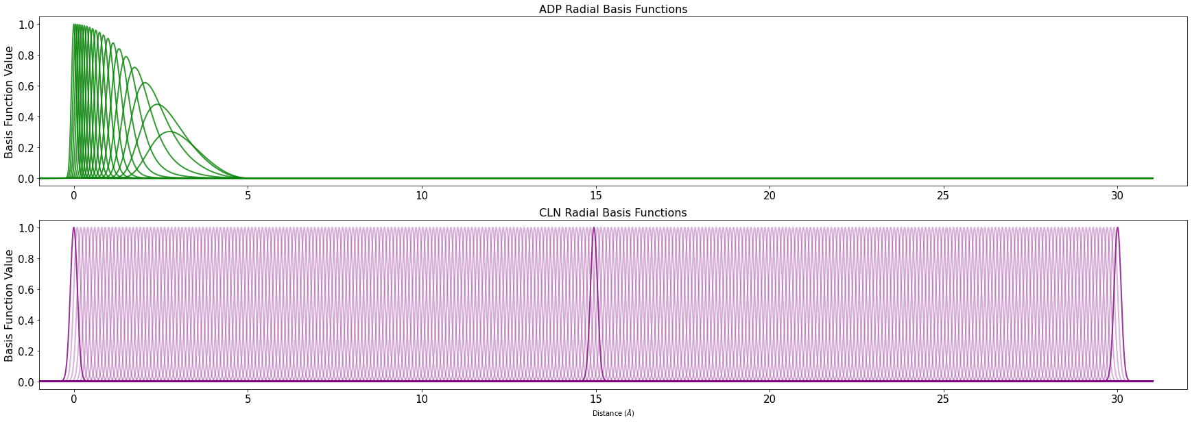
Figure 13: CGSchNet Radial basis function sets for ADP and CLN. For visual clarity, the first, middle, and last basis functions for CLN have been highlighted.

Separate training routines were adopted for each molecule, following the procedure described in Husic et al ⁶⁷. They are reproduced in 4 for convenience.

Hyperparameter	ADP	CLN
Number of Epochs	100	100
Batch Size	512	512
Optimizer	ADAM	ADAM
Weight Initialization	Xavier Uniform	Xavier Uniform
Bias Initialization	Uniform(-$\sqrt{k}$,$\sqrt{k}$)	0
Initial LR	0.0006	0.0001
LR Scheduler	ReduceLROnPlateau	None
Loss Function	MSE Force Matching	MSE Force Matching
Model Selection	Last Epoch	Minimum Average Validation Loss

Table 4: Model Training Hyperparameters

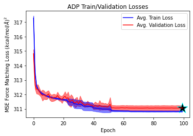
(a)

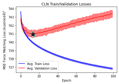
(b)

Figure 14: Epochal training and validation loss curves for the ADP and CLN CGSchNet models over 5 cross validation folds. The solid curves represent the average train/validation loss, while the shaded regions represent a moving standard deviation across the 5 models. The black star represents the epoch at which the final model was chosen.

To assess the performance of each CGSchNet Model, implicit solvent Langevin simulations were carried out with the parameters described in 5.

Parameter	ADP	CLN
Integration Time step	4 fs	4 fs
Friction	1 ps-1	1 ps-1
Initial Structures	Random Sample From Train Set	Random Sample From Train Set
Number of Trajectories	100	1000
Temperature	300K	350K

Table 5: CG Simulation Parameters

For both ADP and CLN, the following BAOA(F)B Langevin scheme was used:

1. $\bar{F}=-\nabla U(x_{t})$

2. $v_{t+1}=v_{t}+dt\frac{\bar{F}}{m}$

3. $x_{t+1/2}=x_{t}+v_{t}\frac{dt}{2}$

4. $v_{t+1}=v_{t+1/2}\eta_{v}+dW_{t}\eta_{n}$

5. $x_{t+1}=x_{t+1/2}v\frac{dt}{2}$

where $\bar{F}$ is an average force predicted by averaging the force predictions from each model produced from cross validation,

$$\bar{F}=\sum_{i=1}^{\text{num folds}}f_{i}$$ (8)

$\eta_{v}$ and $\eta_{n}$ are velocity and noise scales respectively, and $dW$ is a stochastic Wiener process. Forward and backward transitions through all major metastable states are observed in the CG simulations for both molecular systems.

4.3 Latent space embedding and samples

4.4 Alanine dipeptide

Energetics

We notice overall excellent agreement between our atomistic and backmapped ADP trajectories for both the in distribution and generation test sets. This agreement results in nearly identical distributions of the internal potential energy(Fig. 3). The backmapped data tends to slightly deviate by producing small high-energy tails. These rare high-energy configurations produced by our model are a result of a select few bond length and angle distributions that are moderately deformed compared to the reference atomistic data. The largest discrepancies are atomic angles and bonds that include hydrogen atoms, and particularly terminal methyl group hydrogens. While the MD engine restrains all bond lengths involving hydrogen, our model can struggle to exactly reproduce these bond lengths due to the achievable resolution of the voxelized grid. The terminal methy group of ADP is also entirely unspecified by the CG configuration, and methyl group hydrogen atoms are a significant source of variation rotating about the central carbon atom with relaxation times of $\sim$0.1-1 ps which is faster than the 1 ps spacing between consecutive frames ⁹⁷.

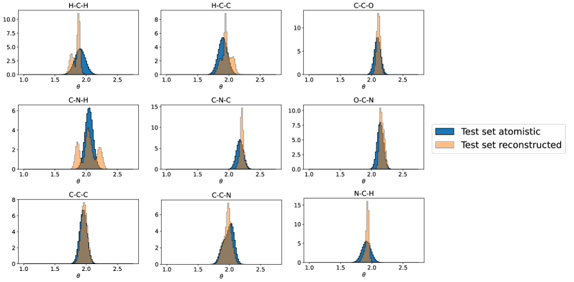
Figure 18: Atomic angle distributions delineated by element participation for the in distribution test set atomistic and backmapped trajectories for ADP.

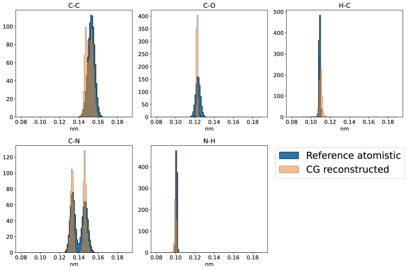
Figure 19: Bond length distributions delineated by element participation for the generalization test reference atomistic and backmapped CGSchNet trajectories for ADP.

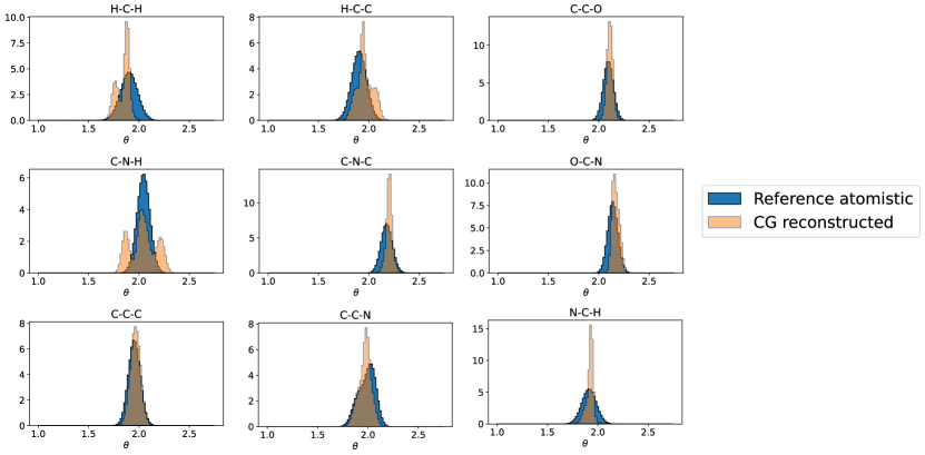
Figure 20: Atomic angle distributions delineated by element participation for the generalization test reference atomistic and backmapped CGSchNet trajectories for ADP.

Thermodynamics

Kinetics

ADP MSM construction and validation

We construct Markov State Models (MSMs) to facilitate the comparison of the kinetics between the reference atomistic data and our backmapped trajectories in Sec. 3.1.3.

We construct MSMs for ADP over the phase space of the backbone $\phi$,$\psi$ angles as they are known to be good CVs for this system. When comparing kinetics between backmapped/CG data and atomistic data we perform k-means clustering for state space decomposition first on the atomistic dataset. We use these same k-means clusters to then produce state assignments for the backmapped/original CG data. Independent MSMs are subsequently fit to the atomistic and backmapped/original CG data from these cluster assignments to ensure direct comparability bewteen the recovered timescales and processes. Associated state space clustering plots, implied timescale analysis for lag time selection and Chapman-Kolmogorow (CK) tests for Markovianity for MSMs built on the different ADP datasets in this work are shown below.

For the in distribution test set we first perform k-means clustering using 100 centroids on the reference atomistic data, the same 100 clusters of which we then also use to build the backmapped in distribution test set MSM.

ADP in distribution test set atomistic

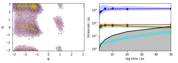
Figure 23: (left) State space clustering using 100 k-means centers fit to the in distribution test set atomistic data shown as orange dots over a contour of the data density. (right) Implied timescale analysis for MSM construction. Solid lines indicate the maximum likelihood MSM estimate, while the dashed lines show the mean implied timescale bounded by a 95% confidence interval. A lag time of 5 ps was selected.

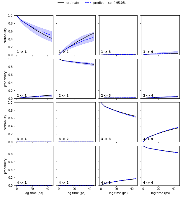
Figure 24: (Chapman-Kolmogorov (CK) test using 4 macrostates. Black lines indicate estimates, while the dashed blue lines are the predictions bounded by a 95% confidence interval)

ADP in distribution test set reconstructed

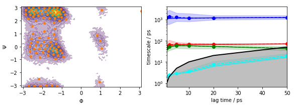
Figure 25: (left) State space clustering of the backmapped in distribution test set using 100 k-means centers taken from the in distribution test set atomistic data shown as orange dots over a contour of the data density. (right) Implied timescale analysis for MSM construction. Solid lines indicate the maximum likelihood MSM estimate, while the dashed lines show the mean implied timescale bounded by a 95% confidence interval. A lag time of 5 ps was selected.

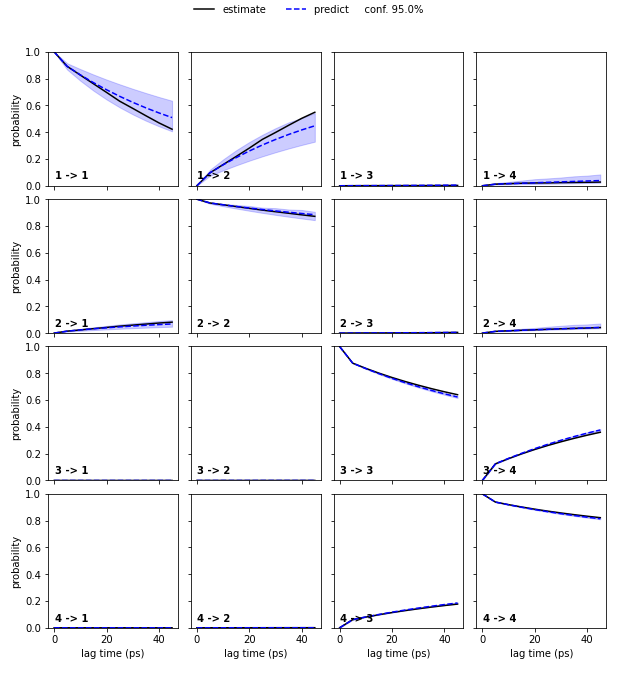
Figure 26: (Chapman-Kolmogorov (CK) test using 4 macrostates. Black lines indicate estimates, while the dashed blue lines are the predictions bounded by a 95% confidence interval)

ADP reference atomistic

For the generalization set we perform state space clustering using 100 kmeans centers first over the reference atomistic dataset which is taken from Ref. ⁷³. These same 100 clusters then define state assignments for MSMs built on both the backmapped CG reconstructed data and the original CGSchNet ⁶⁷ simulation.

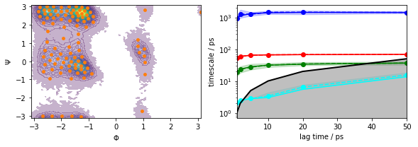
Figure 27: (left) State space clustering using 100 k-means centers fit to the reference atomistic data taken from Ref. ⁷³ shown as orange dots over a contour of the data density. (right) Implied timescale analysis for MSM construction. Solid lines indicate the maximum likelihood MSM estimate, while the dashed lines show the mean implied timescale bounded by a 95% confidence interval. A lag time of 5 ps was selected.

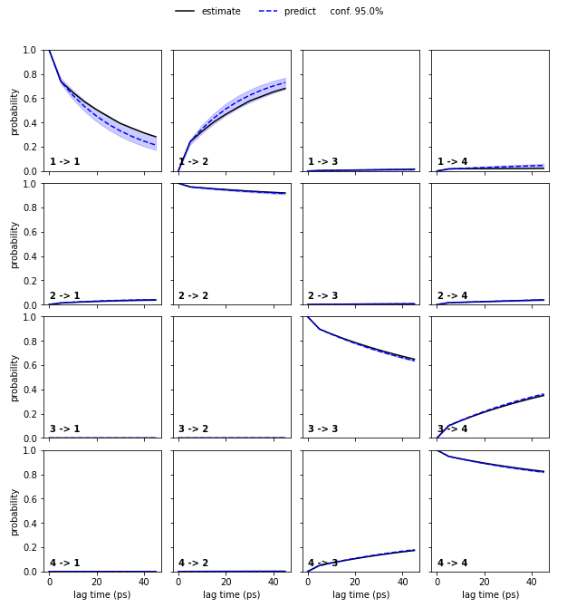
Figure 28: (Chapman-Kolmogorov (CK) test using 4 macrostates. Black lines indicate estimates, while the dashed blue lines are the predictions bounded by a 95% confidence interval)

ADP generalization set reconstructed

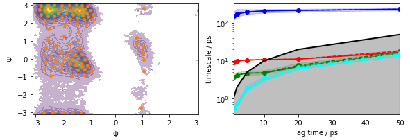
Figure 29: (left) State space clustering of the backmapped CGSchNet data using 100 k-means centers taken from the reference atomistic data shown as orange dots over a contour of the data density. (right) Implied timescale analysis for MSM construction. Solid lines indicate the maximum likelihood MSM estimate, while the dashed lines show the mean implied timescale bounded by a 95% confidence interval. A lag time of 5 ps was selected.

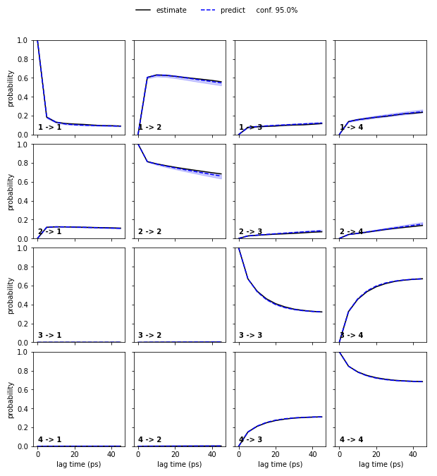
Figure 30: (Chapman-Kolmogorov (CK) test using 4 macrostates. Black lines indicate estimates, while the dashed blue lines are the predictions bounded by a 95% confidence interval)

ADP CGSchNet simulation

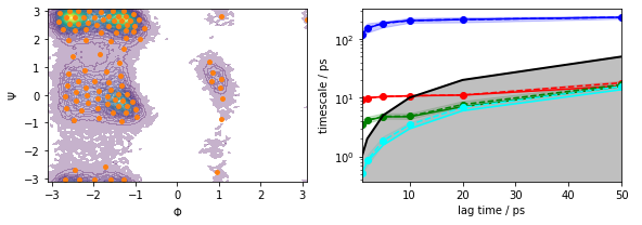
Figure 31: (left) State space clustering of the original coarse grained CGSchNet data using 100 k-means centers taken from the reference atomistic data shown as orange dots over a contour of the data density. (right) Implied timescale analysis for MSM construction. Solid lines indicate the maximum likelihood MSM estimate, while the dashed lines show the mean implied timescale bounded by a 95% confidence interval. A lag time of 5 ps was selected.

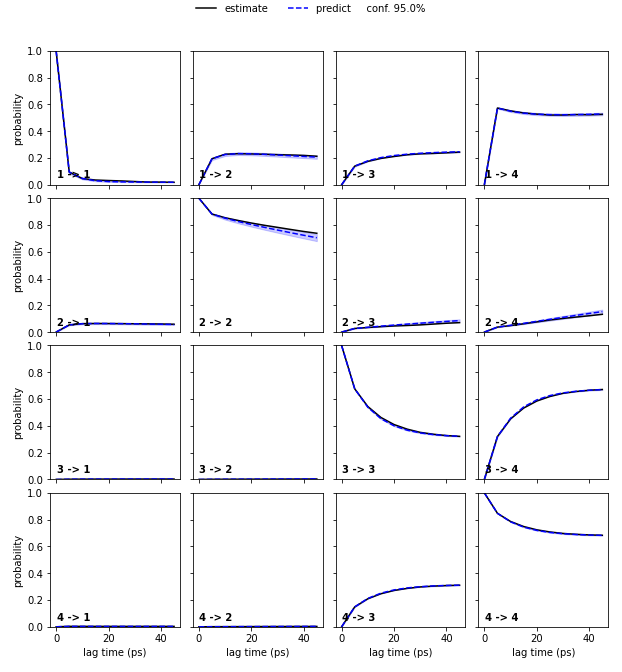
Figure 32: (Chapman-Kolmogorov (CK) test using 4 macrostates. Black lines indicate estimates, while the dashed blue lines are the predictions bounded by a 95% confidence interval)

4.5 Chignolin

Energetics

Thermodynamics

Kinetics

CLN MSM construction and validation

We construct Markov State Models (MSMs) to facilitate the comparison of the kinetics between the reference atomistic data and our backmapped trajectories in Sec. 3.2.3.

To construct MSMs for CLN we first featurize the reference atomistic data taken from Ref. ⁶⁸ using the 45 pairwise $\alpha$-carbon distances between each pair of amino acid residues. We then perform Time-lagged Independent Component Analysis (TICA) on this atomistic data using these pairwise distance features where we retain the first two Independent Components (ICs). We perform state decomposition in this TICA space using k-means clustering with 150 centroids. With the same residue contact featurization for other atomistic, backmapped or CG data we use our learned TICA model to project other data into a common TICA space. Independent MSMs are subsequently built for each separate dataset with state assignments generated in this common TICA space from the same previously identified 150 k-means centers in the reference atomistic dataset. In the case if not all 150 states are occupied MSMs are constructed only using the subset of occupied states for that data set. Operating within this shared TICA and clustering space allows direct comparison between the different MSM recovered timescales and processes. Associated state space clustering plots, implied timescale analysis for lag time selection and Chapman-Kolmogorow (CK) tests for Markovianity for MSMs built on the different CLN datasets in this work are shown below.

CLN reference atomistic

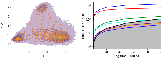
Figure 39: (left) Clustering in TICA space using 150 k-means centers fit to the reference atomistic dataset taken from Ref. ⁶⁸ shown as orange dots over a contour of the data density. (right) Implied timescale analysis for MSM construction. Solid lines indicate the maximum likelihood MSM estimate. A lag time of 4 ns (40 frames) was selected.

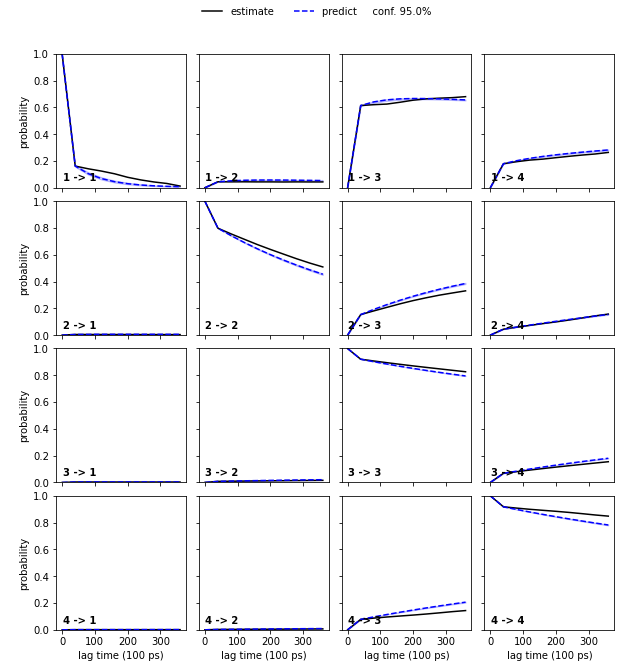
Figure 40: (Chapman-Kolmogorov (CK) test using 4 macrostates. Black lines indicate estimates while the dashed blue lines are the predictions bounded by a 95% confidence interval)

CLN in distribution test set atomistic

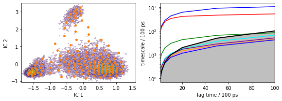
Figure 41: (left) State space clustering for the atomistic in distribution test set data using the same TICA projection and 150 k-means centers from the reference atomistic dataset shown as orange dots over a contour of the data density. (right) Implied timescale analysis for MSM construction. Solid lines indicate the maximum likelihood MSM estimate. A lag time of 4 ns (40 frames) was selected.

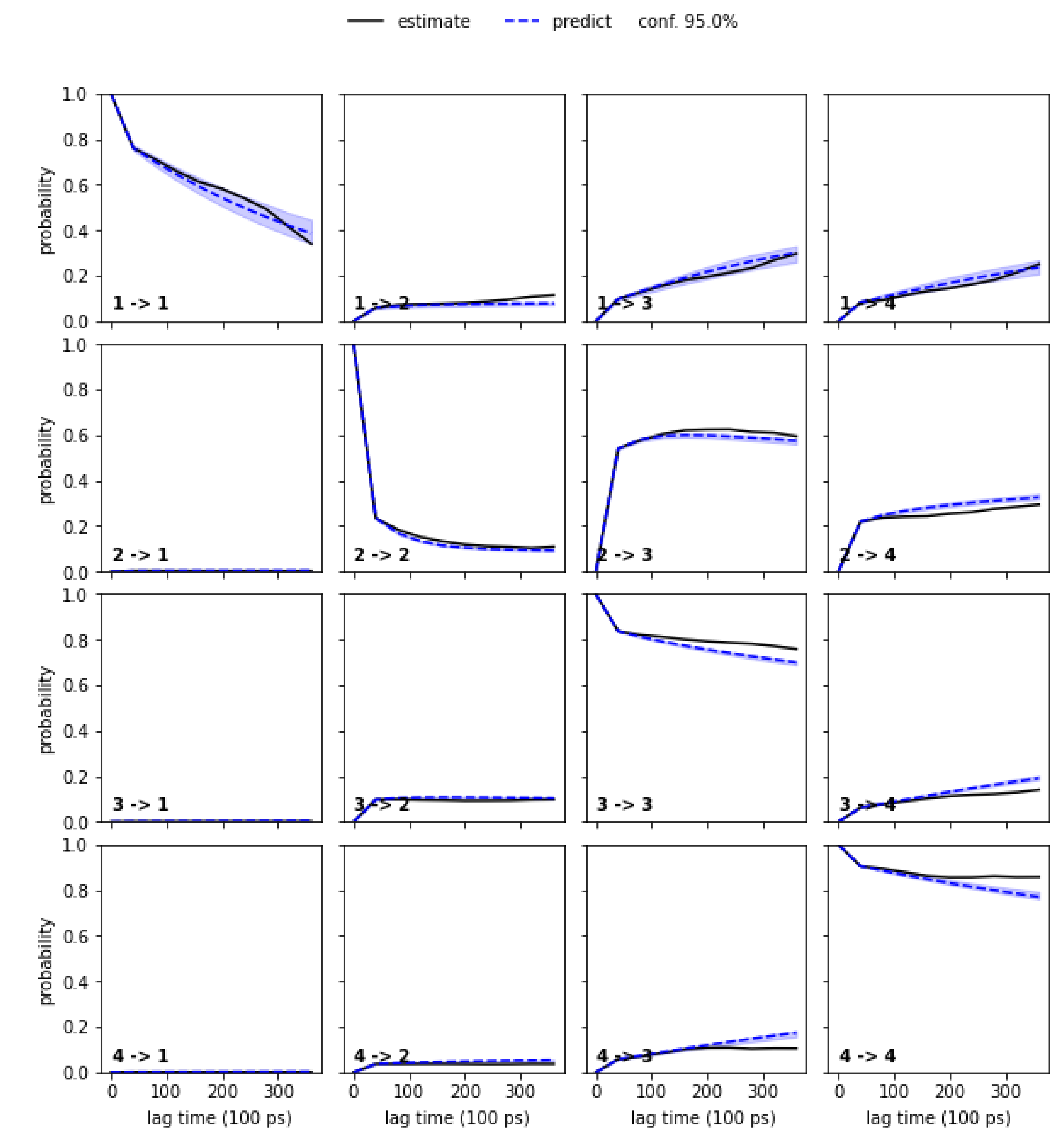
Figure 42: (Chapman-Kolmogorov (CK) test using 4 macrostates. Black lines indicate estimates while the dashed blue lines are the predictions bounded by a 95% confidence interval)

CLN in distribution test set reconstructed

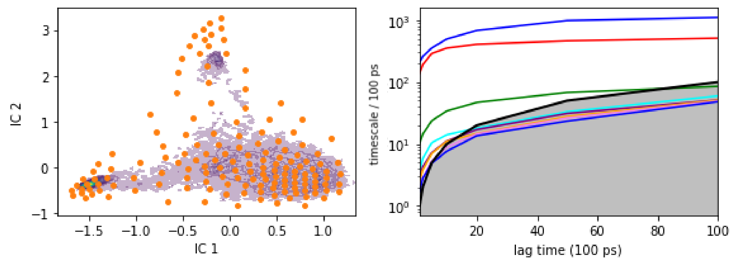
Figure 43: (left) State space clustering for the backmapped in distribution test set data using the same TICA projection and 150 k-means centers from to the reference atomistic dataset shown as orange dots over a contour of the data density. (right) Implied timescale analysis for MSM construction. Solid lines indicate the maximum likelihood MSM estimate. A lag time of 4 ns (40 frames) was selected.

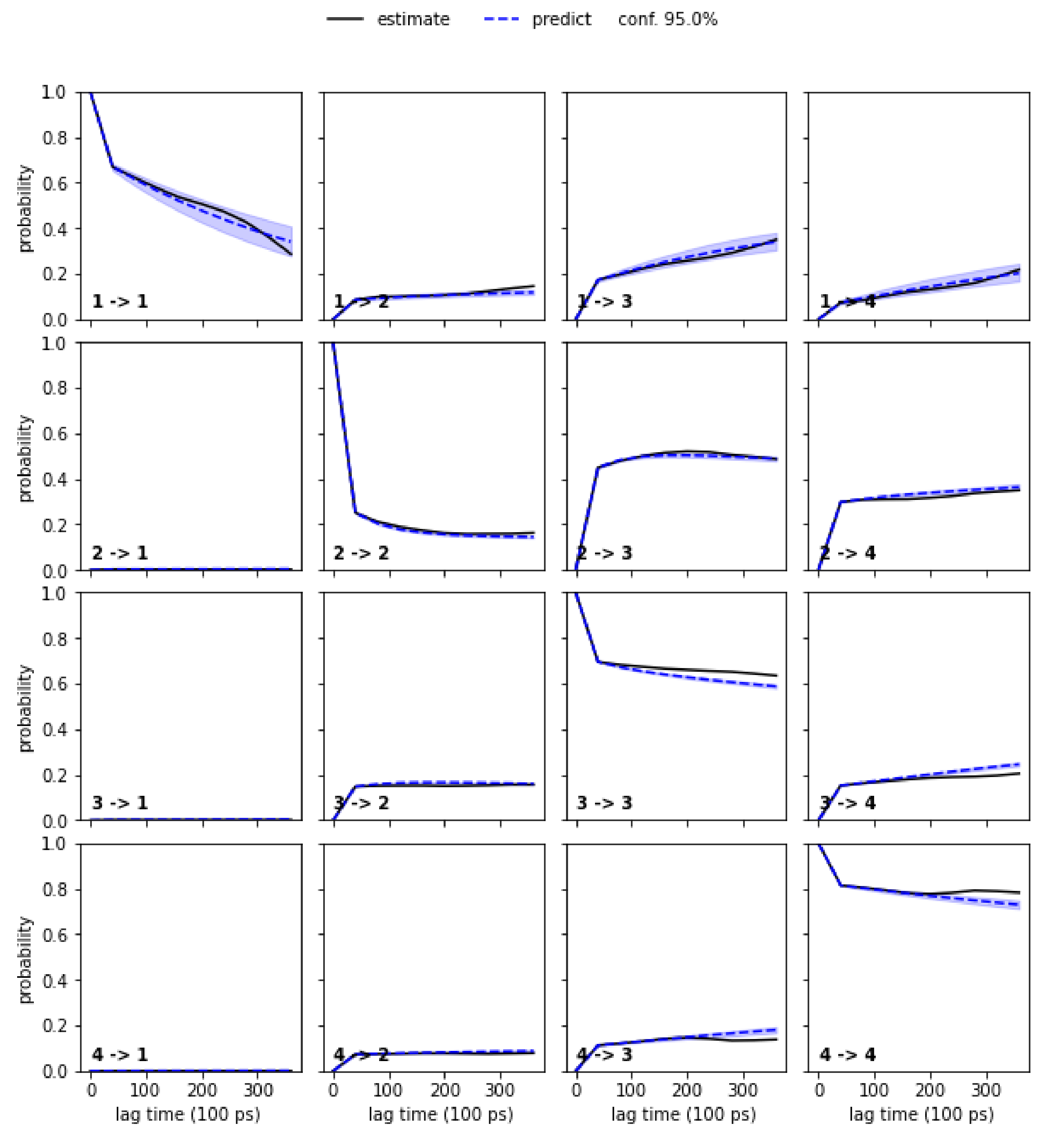
Figure 44: (Chapman-Kolmogorov (CK) test using 4 macrostates. Black lines indicate estimates while the dashed blue lines are the predictions bounded by a 95% confidence interval)

CLN generalization set reconstructed

Figure 45: (left) State space clustering for the backmapped CGSchNet simulation data using the same TICA projection and 150 k-means centers from the reference atomistic dataset shown as orange dots over a contour of the data density. (right) Implied timescale analysis for MSM construction. Solid lines indicate the maximum likelihood MSM estimate. A lag time of 4 ns (40 frames) was selected.

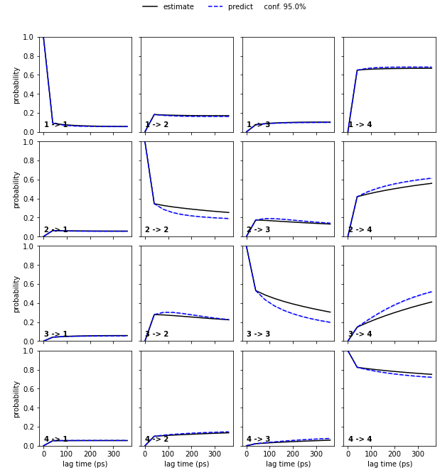
Figure 46: (Chapman-Kolmogorov (CK) test using 4 macrostates. Black lines indicate estimates while the dashed blue lines are the predictions bounded by a 95% confidence interval)

CLN CGSchNet simulation

Figure 47: (left) State space clustering for the original CGSchNet simulation data using the same TICA projection and 150 k-means centers from the reference atomistic dataset shown as orange dots over a contour of the data density. (right) Implied timescale analysis for MSM construction. Solid lines indicate the maximum likelihood MSM estimate. A lag time of 4 ns (40 frames) was selected.

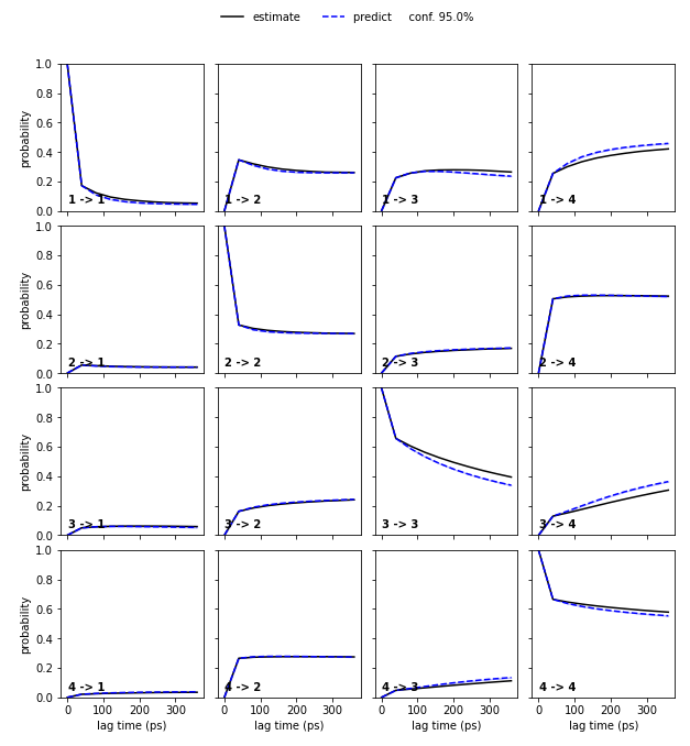
Figure 48: (Chapman-Kolmogorov (CK) test using 4 macrostates. Black lines indicate estimates while the dashed blue lines are the predictions bounded by a 95% confidence interval)

References

- Mitsutake et al. 2013 Mitsutake, A.; Mori, Y.; Okamoto, Y. Biomolecular Simulations; Springer, 2013; pp 153–195
- Bernardi et al. 2015 Bernardi, R. C.; Melo, M. C.; Schulten, K. Enhanced sampling techniques in molecular dynamics simulations of biological systems. Biochimica et Biophysica Acta (BBA)-General Subjects 2015, 1850, 872–877
- Okamoto 2004 Okamoto, Y. Generalized-ensemble algorithms: enhanced sampling techniques for Monte Carlo and molecular dynamics simulations. Journal of Molecular Graphics and Modelling 2004, 22, 425–439
- Sidky et al. 2020 Sidky, H.; Chen, W.; Ferguson, A. L. Machine learning for collective variable discovery and enhanced sampling in biomolecular simulation. Molecular Physics 2020, 118, e1737742
- Noé et al. 2019 Noé, F.; Olsson, S.; Köhler, J.; Wu, H. Boltzmann generators: Sampling equilibrium states of many-body systems with deep learning. Science 2019, 365, eaaw1147
- Shaw et al. 2009 Shaw, D. E.; Dror, R. O.; Salmon, J. K.; Grossman, J.; Mackenzie, K. M.; Bank, J. A.; Young, C.; Deneroff, M. M.; Batson, B.; Bowers, K. J. et al. Millisecond-scale molecular dynamics simulations on Anton. Proceedings of the conference on high performance computing networking, storage and analysis. 2009; pp 1–11
- Hirst et al. 2014 Hirst, J. D.; Glowacki, D. R.; Baaden, M. Molecular simulations and visualization: introduction and overview. Faraday discussions 2014, 169, 9–22
- Shaw et al. 2014 Shaw, D. E.; Grossman, J.; Bank, J. A.; Batson, B.; Butts, J. A.; Chao, J. C.; Deneroff, M. M.; Dror, R. O.; Even, A.; Fenton, C. H. et al. Anton 2: raising the bar for performance and programmability in a special-purpose molecular dynamics supercomputer. SC’14: Proceedings of the International Conference for High Performance Computing, Networking, Storage and Analysis. 2014; pp 41–53
- Kremer and Müller-Plathe 2002 Kremer, K.; Müller-Plathe, F. Multiscale simulation in polymer science. Molecular Simulation 2002, 28, 729–750
- Horstemeyer 2009 Horstemeyer, M. F. Practical aspects of computational chemistry; Springer, 2009; pp 87–135
- Peter and Kremer 2009 Peter, C.; Kremer, K. Multiscale simulation of soft matter systems–from the atomistic to the coarse-grained level and back. Soft Matter 2009, 5, 4357–4366
- Ingólfsson et al. 2014 Ingólfsson, H. I.; Lopez, C. A.; Uusitalo, J. J.; de Jong, D. H.; Gopal, S. M.; Periole, X.; Marrink, S. J. The power of coarse graining in biomolecular simulations. Wiley Interdisciplinary Reviews: Computational Molecular Science 2014, 4, 225–248
- Praprotnik et al. 2008 Praprotnik, M.; Matysiak, S.; Site, L. D.; Kremer, K.; Clementi, C. Adaptive resolution simulation of liquid water. Journal of Physics: Condensed Matter 2008, 21, 499801–499801
- Praprotnik et al. 2005 Praprotnik, M.; Delle Site, L.; Kremer, K. Adaptive resolution molecular-dynamics simulation: Changing the degrees of freedom on the fly. The Journal of Chemical Physics 2005, 123, 224106
- Voth 2008 Voth, G. A. Coarse-graining of condensed phase and biomolecular systems; CRC press, 2008
- Noid 2013 Noid, W. G. Perspective: Coarse-grained models for biomolecular systems. The Journal of chemical physics 2013, 139, 09B201_1
- Brini et al. 2013 Brini, E.; Algaer, E. A.; Ganguly, P.; Li, C.; Rodríguez-Ropero, F.; van der Vegt, N. F. Systematic coarse-graining methods for soft matter simulations–a review. Soft Matter 2013, 9, 2108–2119
- Depa and Maranas 2005 Depa, P. K.; Maranas, J. K. Speed up of dynamic observables in coarse-grained molecular-dynamics simulations of unentangled polymers. The Journal of chemical physics 2005, 123, 094901
- Depa et al. 2011 Depa, P.; Chen, C.; Maranas, J. K. Why are coarse-grained force fields too fast? A look at dynamics of four coarse-grained polymers. The Journal of chemical physics 2011, 134, 014903
- Marrink et al. 2007 Marrink, S. J.; Risselada, H. J.; Yefimov, S.; Tieleman, D. P.; De Vries, A. H. The MARTINI force field: coarse grained model for biomolecular simulations. The journal of physical chemistry B 2007, 111, 7812–7824
- Marrink and Tieleman 2013 Marrink, S. J.; Tieleman, D. P. Perspective on the Martini model. Chemical Society Reviews 2013, 42, 6801–6822
- Nielsen et al. 2004 Nielsen, S. O.; Lopez, C. F.; Srinivas, G.; Klein, M. L. Coarse grain models and the computer simulation of soft materials. Journal of Physics: Condensed Matter 2004, 16, R481
- Baaden and Marrink 2013 Baaden, M.; Marrink, S. J. Coarse-grain modelling of protein–protein interactions. Current opinion in structural biology 2013, 23, 878–886
- Wu and Shea 2011 Wu, C.; Shea, J.-E. Coarse-grained models for protein aggregation. Current opinion in structural biology 2011, 21, 209–220
- Zhang et al. 2019 Zhang, G.; Chazirakis, A.; Harmandaris, V. A.; Stuehn, T.; Daoulas, K. C.; Kremer, K. Hierarchical modelling of polystyrene melts: from soft blobs to atomistic resolution. Soft Matter 2019, 15, 289–302
- Srinivas et al. 2004 Srinivas, G.; Discher, D. E.; Klein, M. L. Self-assembly and properties of diblock copolymers by coarse-grain molecular dynamics. Nature materials 2004, 3, 638–644
- Shmilovich et al. 2020 Shmilovich, K.; Mansbach, R. A.; Sidky, H.; Dunne, O. E.; Panda, S. S.; Tovar, J. D.; Ferguson, A. L. Discovery of self-assembling -conjugated peptides by active learning-directed coarse-grained molecular simulation. The Journal of Physical Chemistry B 2020, 124, 3873–3891
- Mohr et al. 2022 Mohr, B.; Shmilovich, K.; Kleinwächter, I. S.; Schneider, D.; Ferguson, A. L.; Bereau, T. Data-driven discovery of cardiolipin-selective small molecules by computational active learning. Chemical Science 2022,
- Sadeghi and Noé 2020 Sadeghi, M.; Noé, F. Large-scale simulation of biomembranes incorporating realistic kinetics into coarse-grained models. Nature communications 2020, 11, 1–13
- Bradley and Radhakrishnan 2013 Bradley, R.; Radhakrishnan, R. Coarse-grained models for protein-cell membrane interactions. Polymers 2013, 5, 890–936
- Wang et al. 2018 Wang, J.; Gayatri, M.; Ferguson, A. L. Coarse-grained molecular simulation and nonlinear manifold learning of archipelago asphaltene aggregation and folding. The Journal of Physical Chemistry B 2018, 122, 6627–6647
- Helgaker et al. 2014 Helgaker, T.; Jorgensen, P.; Olsen, J. Molecular electronic-structure theory; John Wiley & Sons, 2014
- McQuarrie and Simon 1997 McQuarrie, D. A.; Simon, J. D. Physical chemistry: a molecular approach; University science books Sausalito, CA, 1997; Vol. 1
- Hess et al. 2006 Hess, B.; León, S.; Van Der Vegt, N.; Kremer, K. Long time atomistic polymer trajectories from coarse grained simulations: bisphenol-A polycarbonate. Soft Matter 2006, 2, 409–414
- Rzepiela et al. 2010 Rzepiela, A. J.; Schäfer, L. V.; Goga, N.; Risselada, H. J.; De Vries, A. H.; Marrink, S. J. Reconstruction of atomistic details from coarse-grained structures. Journal of computational chemistry 2010, 31, 1333–1343
- Wassenaar et al. 2014 Wassenaar, T. A.; Pluhackova, K.; Bockmann, R. A.; Marrink, S. J.; Tieleman, D. P. Going backward: a flexible geometric approach to reverse transformation from coarse grained to atomistic models. Journal of chemical theory and computation 2014, 10, 676–690
- Heath et al. 2007 Heath, A. P.; Kavraki, L. E.; Clementi, C. From coarse-grain to all-atom: Toward multiscale analysis of protein landscapes. Proteins: Structure, Function, and Bioinformatics 2007, 68, 646–661
- Stieffenhofer et al. 2020 Stieffenhofer, M.; Wand, M.; Bereau, T. Adversarial reverse mapping of equilibrated condensed-phase molecular structures. Machine Learning: Science and Technology 2020, 1, 045014
- Stieffenhofer et al. 2021 Stieffenhofer, M.; Bereau, T.; Wand, M. Adversarial reverse mapping of condensed-phase molecular structures: Chemical transferability. APL Materials 2021, 9, 031107
- Wang and Gómez-Bombarelli 2019 Wang, W.; Gómez-Bombarelli, R. Coarse-graining auto-encoders for molecular dynamics. npj Computational Materials 2019, 5, 1–9
- Li et al. 2020 Li, W.; Burkhart, C.; Polińska, P.; Harmandaris, V.; Doxastakis, M. Backmapping coarse-grained macromolecules: An efficient and versatile machine learning approach. The Journal of Chemical Physics 2020, 153, 041101
- An and Deshmukh 2020 An, Y.; Deshmukh, S. A. Machine learning approach for accurate backmapping of coarse-grained models to all-atom models. Chemical Communications 2020, 56, 9312–9315
- Wang et al. 2022 Wang, W.; Xu, M.; Cai, C.; Miller, B. K.; Smidt, T.; Wang, Y.; Tang, J.; Gómez-Bombarelli, R. Generative Coarse-Graining of Molecular Conformations. arXiv preprint arXiv:2201.12176 2022,
- Frenkel and Smit 2001 Frenkel, D.; Smit, B. Understanding molecular simulation: from algorithms to applications; Elsevier, 2001; Vol. 1
- Bergsma et al. 1984 Bergsma, J. P.; Berens, P. H.; Wilson, K. R.; Fredkin, D. R.; Heller, E. J. Electronic spectra from molecular dynamics: a simple approach. The Journal of Physical Chemistry 1984, 88, 612–619
- Guillot 1991 Guillot, B. A molecular dynamics study of the far infrared spectrum of liquid water. The Journal of chemical physics 1991, 95, 1543–1551
- Salacuse et al. 1996 Salacuse, J. J.; Denton, A. R.; Egelstaff, P. A. Finite-size effects in molecular dynamics simulations: Static structure factor and compressibility. I. Theoretical method. Phys. Rev. E 1996, 53, 2382–2389
- Moe and Ediger 1999 Moe, N. E.; Ediger, M. Calculation of the coherent dynamic structure factor of polyisoprene from molecular dynamics simulations. Physical Review E 1999, 59, 623
- Chen et al. 2008 Chen, C.; Depa, P.; Maranas, J. K.; Garcia Sakai, V. Comparison of explicit atom, united atom, and coarse-grained simulations of poly (methyl methacrylate). The Journal of chemical physics 2008, 128, 124906
- Arbe et al. 2012 Arbe, A.; Alvarez, F.; Colmenero, J. Neutron scattering and molecular dynamics simulations: Synergetic tools to unravel structure and dynamics in polymers. Soft Matter 2012, 8, 8257–8270
- Paszke et al. 2019 Paszke, A.; Gross, S.; Massa, F.; Lerer, A.; Bradbury, J.; Chanan, G.; Killeen, T.; Lin, Z.; Gimelshein, N.; Antiga, L. et al. Pytorch: An imperative style, high-performance deep learning library. Advances in neural information processing systems 2019, 32
- Shmilovich et al. 2022 Shmilovich, K.; Stieffenhofer, M.; Charron, N. E.; Hoffmann, M. Supporting data for "Temporally coherent backmapping of molecular trajectories from coarse-grain to atomistic resolution". 2022; https://petreldata.net/mdf/detail/shmilovich_supporting_temporally_resolution_v1.6
- Fukushima et al. 1983 Fukushima, K.; Miyake, S.; Ito, T. Neocognitron: A neural network model for a mechanism of visual pattern recognition. IEEE transactions on systems, man, and cybernetics 1983, 826–834
- LeCun et al. 1989 LeCun, Y.; Boser, B.; Denker, J. S.; Henderson, D.; Howard, R. E.; Hubbard, W.; Jackel, L. D. Backpropagation applied to handwritten zip code recognition. Neural computation 1989, 1, 541–551
- LeCun et al. 1998 LeCun, Y.; Bottou, L.; Bengio, Y.; Haffner, P. Gradient-based learning applied to document recognition. Proceedings of the IEEE 1998, 86, 2278–2324
- Rawat and Wang 2017 Rawat, W.; Wang, Z. Deep convolutional neural networks for image classification: A comprehensive review. Neural computation 2017, 29, 2352–2449
- Voulodimos et al. 2018 Voulodimos, A.; Doulamis, N.; Doulamis, A.; Protopapadakis, E. Deep learning for computer vision: A brief review. Computational intelligence and neuroscience 2018, 2018
- Sohn et al. 2015 Sohn, K.; Lee, H.; Yan, X. Learning structured output representation using deep conditional generative models. Advances in neural information processing systems 2015, 28
- Kingma and Welling 2013 Kingma, D. P.; Welling, M. Auto-encoding variational bayes. arXiv preprint arXiv:1312.6114 2013,
- Kingma and Ba 2014 Kingma, D. P.; Ba, J. Adam: A method for stochastic optimization. arXiv preprint arXiv:1412.6980 2014,
- Fu et al. 2019 Fu, H.; Li, C.; Liu, X.; Gao, J.; Celikyilmaz, A.; Carin, L. Cyclical annealing schedule: A simple approach to mitigating kl vanishing. arXiv preprint arXiv:1903.10145 2019,
- Ghosh et al. 2019 Ghosh, P.; Sajjadi, M. S.; Vergari, A.; Black, M.; Schölkopf, B. From variational to deterministic autoencoders. arXiv preprint arXiv:1903.12436 2019,
- Eastman et al. 2017 Eastman, P.; Swails, J.; Chodera, J. D.; McGibbon, R. T.; Zhao, Y.; Beauchamp, K. A.; Wang, L.-P.; Simmonett, A. C.; Harrigan, M. P.; Stern, C. D. et al. OpenMM 7: Rapid development of high performance algorithms for molecular dynamics. PLoS computational biology 2017, 13, e1005659
- Nüske et al. 2017 Nüske, F.; Wu, H.; Prinz, J.-H.; Wehmeyer, C.; Clementi, C.; Noé, F. Markov state models from short non-equilibrium simulations—Analysis and correction of estimation bias. The Journal of Chemical Physics 2017, 146, 094104
- Lindorff-Larsen et al. 2010 Lindorff-Larsen, K.; Piana, S.; Palmo, K.; Maragakis, P.; Klepeis, J. L.; Dror, R. O.; Shaw, D. E. Improved side-chain torsion potentials for the Amber ff99SB protein force field. Proteins: Structure, Function, and Bioinformatics 2010, 78, 1950–1958
- Darden et al. 1993 Darden, T.; York, D.; Pedersen, L. Particle mesh Ewald: An N log (N) method for Ewald sums in large systems. The Journal of chemical physics 1993, 98, 10089–10092
- Husic et al. 2020 Husic, B. E.; Charron, N. E.; Lemm, D.; Wang, J.; Pérez, A.; Majewski, M.; Krämer, A.; Chen, Y.; Olsson, S.; de Fabritiis, G. et al. Coarse graining molecular dynamics with graph neural networks. The Journal of chemical physics 2020, 153, 194101
- Wang et al. 2019 Wang, J.; Olsson, S.; Wehmeyer, C.; Pérez, A.; Charron, N. E.; De Fabritiis, G.; Noé, F.; Clementi, C. Machine learning of coarse-grained molecular dynamics force fields. ACS central science 2019, 5, 755–767
- Harvey et al. 2009 Harvey, M. J.; Giupponi, G.; Fabritiis, G. D. ACEMD: accelerating biomolecular dynamics in the microsecond time scale. Journal of chemical theory and computation 2009, 5, 1632–1639
- Buch et al. 2010 Buch, I.; Harvey, M. J.; Giorgino, T.; Anderson, D. P.; De Fabritiis, G. High-throughput all-atom molecular dynamics simulations using distributed computing. Journal of chemical information and modeling 2010, 50, 397–403
- Lindorff-Larsen et al. 2011 Lindorff-Larsen, K.; Piana, S.; Dror, R. O.; Shaw, D. E. How fast-folding proteins fold. Science 2011, 334, 517–520
- Doerr and De Fabritiis 2014 Doerr, S.; De Fabritiis, G. On-the-fly learning and sampling of ligand binding by high-throughput molecular simulations. Journal of chemical theory and computation 2014, 10, 2064–2069
- Wehmeyer and Noé 2018 Wehmeyer, C.; Noé, F. Time-lagged autoencoders: Deep learning of slow collective variables for molecular kinetics. The Journal of chemical physics 2018, 148, 241703
- Nuske et al. 2014 Nuske, F.; Keller, B. G.; Pérez-Hernández, G.; Mey, A. S.; Noé, F. Variational approach to molecular kinetics. Journal of chemical theory and computation 2014, 10, 1739–1752
- Vitalini et al. 2015 Vitalini, F.; Mey, A. S.; Noé, F.; Keller, B. G. Dynamic properties of force fields. The Journal of Chemical Physics 2015, 142, 02B611_1
- Prinz et al. 2011 Prinz, J.-H.; Wu, H.; Sarich, M.; Keller, B.; Senne, M.; Held, M.; Chodera, J. D.; Schütte, C.; Noé, F. Markov models of molecular kinetics: Generation and validation. The Journal of chemical physics 2011, 134, 174105
- Bowman et al. 2013 Bowman, G. R.; Pande, V. S.; Noé, F. An introduction to Markov state models and their application to long timescale molecular simulation; Springer Science & Business Media, 2013; Vol. 797
- Trendelkamp-Schroer et al. 2015 Trendelkamp-Schroer, B.; Wu, H.; Paul, F.; Noé, F. Estimation and uncertainty of reversible Markov models. The Journal of chemical physics 2015, 143, 11B601_1
- Scherer et al. 2015 Scherer, M. K.; Trendelkamp-Schroer, B.; Paul, F.; Pérez-Hernández, G.; Hoffmann, M.; Plattner, N.; Wehmeyer, C.; Prinz, J.-H.; Noé, F. PyEMMA 2: A software package for estimation, validation, and analysis of Markov models. Journal of chemical theory and computation 2015, 11, 5525–5542
- Hoffmann et al. 2021 Hoffmann, M.; Scherer, M.; Hempel, T.; Mardt, A.; de Silva, B.; Husic, B. E.; Klus, S.; Wu, H.; Kutz, N.; Brunton, S. L. et al. Deeptime: a Python library for machine learning dynamical models from time series data. Machine Learning: Science and Technology 2021, 3, 015009
- Fritz et al. 2011 Fritz, D.; Koschke, K.; Harmandaris, V. A.; van der Vegt, N. F.; Kremer, K. Multiscale modeling of soft matter: scaling of dynamics. Physical Chemistry Chemical Physics 2011, 13, 10412–10420
- Pérez-Hernández et al. 2013 Pérez-Hernández, G.; Paul, F.; Giorgino, T.; De Fabritiis, G.; Noé, F. Identification of slow molecular order parameters for Markov model construction. The Journal of chemical physics 2013, 139, 07B604_1
- Wu and Noé 2020 Wu, H.; Noé, F. Variational approach for learning Markov processes from time series data. Journal of Nonlinear Science 2020, 30, 23–66
- Noé and Clementi 2015 Noé, F.; Clementi, C. Kinetic distance and kinetic maps from molecular dynamics simulation. Journal of chemical theory and computation 2015, 11, 5002–5011
- Chen et al. 2021 Chen, Y.; Krämer, A.; Charron, N. E.; Husic, B. E.; Clementi, C.; Noé, F. Machine learning implicit solvation for molecular dynamics. The Journal of Chemical Physics 2021, 155, 084101
- Köhler et al. 2022 Köhler, J.; Chen, Y.; Krämer, A.; Clementi, C.; Noé, F. Force-matching Coarse-Graining without Forces. 2022; https://arxiv.org/abs/2203.11167
- Miller et al. 2020 Miller, B. K.; Geiger, M.; Smidt, T. E.; Noé, F. Relevance of rotationally equivariant convolutions for predicting molecular properties. arXiv preprint arXiv:2008.08461 2020,
- Thomas et al. 2018 Thomas, N.; Smidt, T.; Kearnes, S.; Yang, L.; Li, L.; Kohlhoff, K.; Riley, P. Tensor field networks: Rotation-and translation-equivariant neural networks for 3d point clouds. arXiv preprint arXiv:1802.08219 2018,
- Batzner et al. 2021 Batzner, S.; Musaelian, A.; Sun, L.; Geiger, M.; Mailoa, J. P.; Kornbluth, M.; Molinari, N.; Smidt, T. E.; Kozinsky, B. Se (3)-equivariant graph neural networks for data-efficient and accurate interatomic potentials. arXiv preprint arXiv:2101.03164 2021,
- Blaiszik et al. 2016 Blaiszik, B.; Chard, K.; Pruyne, J.; Ananthakrishnan, R.; Tuecke, S.; Foster, I. The materials data facility: data services to advance materials science research. JOM: The Journal of The Minerals, Metals & Materials Society (TMS) 2016, 68, 2045–2052
- Blaiszik et al. 2019 Blaiszik, B.; Ward, L.; Schwarting, M.; Gaff, J.; Chard, R.; Pike, D.; Chard, K.; Foster, I. A data ecosystem to support machine learning in materials science. MRS Communications 2019, 9, 1125–1133
- Brooks et al. 2009 Brooks, B. R.; Brooks III, C. L.; Mackerell Jr, A. D.; Nilsson, L.; Petrella, R. J.; Roux, B.; Won, Y.; Archontis, G.; Bartels, C.; Boresch, S. et al. CHARMM: the biomolecular simulation program. Journal of computational chemistry 2009, 30, 1545–1614
- Lee et al. 2016 Lee, J.; Cheng, X.; Swails, J. M.; Yeom, M. S.; Eastman, P. K.; Lemkul, J. A.; Wei, S.; Buckner, J.; Jeong, J. C.; Qi, Y. et al. CHARMM-GUI input generator for NAMD, GROMACS, AMBER, OpenMM, and CHARMM/OpenMM simulations using the CHARMM36 additive force field. Journal of chemical theory and computation 2016, 12, 405–413
- Jo et al. 2008 Jo, S.; Kim, T.; Iyer, V. G.; Im, W. CHARMM-GUI: a web-based graphical user interface for CHARMM. Journal of computational chemistry 2008, 29, 1859–1865
- Falcon et al. 2019 Falcon, W., et al. Pytorch lightning. GitHub. Note: https://github. com/PyTorchLightning/pytorch-lightning 2019, 3, 6
- Doerr et al. 2021 Doerr, S.; Majewski, M.; Pérez, A.; Kramer, A.; Clementi, C.; Noe, F.; Giorgino, T.; De Fabritiis, G. Torchmd: A deep learning framework for molecular simulations. Journal of chemical theory and computation 2021, 17, 2355–2363
- Yi et al. 2013 Yi, Z.; Lindner, B.; Prinz, J.-H.; Noé, F.; Smith, J. C. Dynamic neutron scattering from conformational dynamics. II. Application using molecular dynamics simulation and Markov modeling. The Journal of Chemical Physics 2013, 139, 11B601_1