Parallel Private Retrieval of Merkle Proofs
via Tree Colorings

Abstract

Motivated by a practical scenario in blockchains in which a client, who possesses a transaction, wishes to privately verify that the transaction actually belongs to a block, we investigate the problem of private retrieval of Merkle proofs (i.e. proofs of inclusion/membership) in a Merkle tree. In this setting, one or more servers store the nodes of a binary tree (a Merkle tree), while a client wants to retrieve the set of nodes along a root-to-leaf path (i.e. a Merkle proof, after appropriate node swapping operations), without letting the servers know which path is being retrieved. We propose a method that partitions the Merkle tree to enable parallel private retrieval of the Merkle proofs. The partitioning step is based on a novel tree coloring called ancestral coloring in which nodes with ancestor-descendant relationship must have distinct colors. To minimize the retrieval time, the coloring must be balanced, i.e. the sizes of the color classes must differ by at most one. We develop a fast algorithm to find a balanced ancestral coloring in almost linear time in the number of tree nodes, which can handle trees with billions of nodes in minutes. Unlike existing approaches, ours allows an efficient indexing with polylog time and space complexity. Our partitioning method can be applied on top of any private information retrieval scheme, leading to the minimum storage overhead and fastest running time compared to existing works.

I Introduction

A Merkle tree is a binary tree (dummy items can be padded to make the tree perfect) in which each node is the (cryptographic) hash of the concatenation of the contents of its child nodes [1]. A Merkle tree can be used to store a large number of data items in a way that not only guarantees data integrity but also allows a very efficient membership verification, which can be performed with complexity $\log(n)$ where $n$ is the number of items stored by the tree at the leaf nodes. More specifically, the membership verification of an item uses its Merkle proof defined as follows: the Merkle proof corresponding to the item stored at a leaf node consists of $\log(n)$ hashes stored at the siblings of the nodes in the path from that leaf node to the root (see Fig. 1 for a toy example). Here, by convention, the root node is the sibling of itself. Due to their simple construction and powerful features, Merkle trees have been widely used in practice, e.g., for data synchronization in Amazon DynamoDB [2], for certificates storage in Google’s Certificate Transparency [3], and transactions storage in blockchains [4, 5].

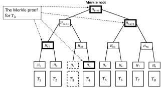
Figure 1: Illustration of a Merkle tree that stores eight transactions $T_{1},T_{2},\ldots,T_{8}$. The leaf nodes of the tree store the hashes of these transactions, i.e., $H_{1}=H(T_{1}),\ldots,H_{8}=H(T_{8})$, where $H(\cdot)$ is a cryptographic hash function. Each non-leaf node is created by hashing the concatenation of the hashes stored at its two child nodes. For instance, $H_{12}=H(H_{1}||H_{2})$, and $H_{1234}=H(H_{12}||H_{34})$. The Merkle proof of the transaction $T_{3}$ consists of $H_{4},H_{12},H_{5678}$, and $H_{1-8}$, that is, all the hashes stored at the siblings of nodes along the path from $H_{3}$ up to the root.

In this work, we are interested in the problem of private retrieval of Merkle proofs from a Merkle tree described as follows. Suppose that a database consisting of $n$ items $(T_{i})_{i=1}^{n}$ is stored in a Merkle tree of height $h$ and that the Merkle root (root hash) is made public. We also assume that the Merkle tree is collectively stored at one or more servers. The goal is to design a retrieval scheme that allows a client who owns one item $T_{i}$ to retrieve its corresponding Merkle proof (in order to verify if $T_{i}$ indeed belongs to the tree) without revealing $i$ to the servers that store the Merkle tree.

The problem of private retrieval of Merkle proofs defined above has a direct application in all systems that use Merkle tree to store data, in particular, blockchains, in which privacy has always been a pressing issue [6, 7, 8]. For example, a solution to this problem allows a client who has a transaction to privately verify whether the transaction belongs to a certain block or not by privately downloading the Merkle proof of the transaction from one or more full nodes storing the corresponding block. In the context of website certificates [9], such a solution allows a web client to verify with a log server whether the certificate of a website is indeed valid (i.e., included in the log) without revealing which website it is visiting (see [10, 11] for more detailed discussion).

Assuming a setting in which a single multi-core server or multiple (single-core) servers are available, we propose a method to parallelize the retrieval process on the Merkle tree, which significantly speeds up the process. Our main idea is to first partition the set of nodes of the Merkle tree into $h=\log(n)$ parts (i.e. sub-databases) so that each part contains exactly one node in the Merkle proof, and then let the client run a private information retrieval scheme (see [12, 13]) in each part and retrieve the corresponding node. Moreover, to avoid any bottleneck, we must balance the workload among the cores/servers. This translates to the second property of the tree partition: the parts of the partitions must have more or less the same sizes. We discuss below the concept of private information retrieval (PIR) and demonstrate the reason why a partition of the tree that violates the first property defined above may break the retrieval privacy and reveal the identity of the item corresponding to the Merkle proof.

Private information retrieval (PIR) was first introduced in the seminal work of Chor-Goldreich-Kushilevitz-Sudan [12], followed by Kushilevitz-Ostrovsky [13], and has been extensively studied in the literature. A PIR scheme allows a client to retrieve an item $x_{j}$ in a database $\{x_{1},x_{2},\ldots,x_{N}\}$ stored by one or several servers without revealing the item index $j$. Two well-known classes of PIR schemes, namely information-theoretic PIR (IT-PIR) (see, e.g. [12, 14, 15]) and computational PIR (CPIR) (see, e.g. [13, 16, 17, 18, 19, 20]) have been developed to minimize the communication overhead between clients and servers. Recently, researchers have also constructed PIR schemes that aim to optimize the download cost for databases with large-size items (see, e.g. [21, 22]). Last but not least, PIR schemes that allow the client to verify and/or correct the retrieved result, assuming the presence of malicious server(s), have also been investigated [23, 24, 25, 26, 27, 28, 29, 30, 31, 32, 33, 34, 35, 36, 37].

In our proposed tree-partitioning based approach to parallelize the retrieval of a Merkle proof, as previously mentioned, we require that each part of the partition contains precisely one tree node in the Merkle proof. This property of the partition not only contributes to balanced communication and computation loads among the cores/servers, but also plays an essential role in ensuring the privacy of the item/Merkle proof. To justify this property, we demonstrate in Fig. 2 a “bad” tree partition with $h=3$ parts labeled by R (Red), G (Green), and B (Blue), which breaks the privacy. Indeed, the Merkle proof for $T_{3}$ (excluding the root node) consists of two G nodes, which means that the core/server handling the G part (regarded as a PIR sub-database) will receive two PIR requests from the client, which allows it to conclude that the Merkle proof must be for $T_{3}$. The reason is that no other Merkle proofs contain two G nodes. In fact, it can be easily verified by inspection that all other seven Merkle proofs contain exactly one node from each part R, G, and B. Note that this property is not only necessary but also sufficient to guarantee the privacy of the downloaded Merkle proof: on each part (treated as an independent sub-database), the PIR scheme ensures that the core/server cannot find out which node is being retrieved; as any valid combination of $h$ nodes is possible (there are $n=2^{h}$ such combinations, corresponding to $2^{n}$ proofs/items), the servers cannot identify the proof being retrieved.

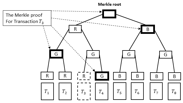
Figure 2: An example of a (balanced) tree partition that breaks the privacy of the retrieval scheme. The set of tree nodes is partitioned into three balanced parts: R (Red), G (Green), and B (Blue). Suppose the Merkle proof for $T_{3}$ is being downloaded. We can exclude the root because it is a public knowledge. Although the PIR scheme itself applied to each part (sub-database) doesn’t reveal the nodes being downloaded, the fact that this Merkle proof contains two G nodes will break the privacy: the core/server can tell that the proof corresponds to $T_{3}$ because it is the only one that contains two G nodes, which requires two requests made to the core/server processing the G part.

Having identified the key property that is essential for a tree partitioning to preserve privacy, our second contribution is to formalize the property by introducing a novel concept of ancestral coloring for rooted trees. We first observe that the nodes in a Merkle proof of a Merkle tree, treating as a perfect binary tree (by adding dummy items if necessary), correspond to tree nodes along a root-to-leaf path (excluding the root) in the swapped Merkle tree in which sibling nodes are swapped (see Fig. 4). Hence, the problem of privately retrieving a Merkle proof is reduced to the equivalent problem of privately retrieving all nodes along a root-to-leaf path in a perfect binary tree. In our proposed tree coloring problem, one seeks to color (i.e. partition) the tree nodes using $h$ different colors labeled $1,2,\ldots,h$ such that nodes on every root-to-leaf path in the tree have distinct colors, except for the root node (which is colorless). This property is called the Ancestral Property as it ensures that nodes with ancestor-descendant relationship must have different colors. Equivalently, the Ancestral Property requires that each of the $h$ color classes $C_{i}$ (i.e. each part of the partition) contains exactly one node from every Merkle proof. A coloring $\mathcal{C}=\{C_{1},C_{2},\ldots,C_{h}\}$ of a tree that satisfies the Ancestral Property is called an ancestral coloring.

To minimize the concurrent execution time and storage overhead of the server(s), we also consider the Balanced Property for the ancestral colorings, which ensures that the sizes $|C_{i}|$ of the $h$ color classes (sub-databases) $C_{i}$, $i=1,2,\ldots,h$, are different by at most one. An ancestral coloring $C$ of a rooted tree that also satisfies the Balanced Property is called a balanced ancestral coloring. A trivial ancestral coloring is the layer-based coloring, i.e., for a perfect binary tree with nodes index by $1,2,\ldots$ and 1 as the root node, $C_{1}=\{2,3\}$ (first layer), $C_{2}=\{4,5,6,7\}$ (second layer), etc. However, this trivial ancestral coloring is not balanced. We illustrate in Fig. 3 examples of balanced ancestral colorings for the perfect binary trees $T(h)$ when $h=1,2,3$. Note that these colorings may not be unique, and different balanced ancestral colorings for $T(h)$ can be constructed when $h\geq 3$. Constructing balanced ancestral colorings (if any), or more generally, ancestral colorings with given color class sizes $c_{i}=|C_{i}|$ ($1\leq i\leq h$), for every rooted tree, is a highly challenging task. In the scope of this work, we focus on perfect binary trees, which is sufficient for the applications using Merkle trees.

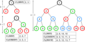
Figure 3: Balanced ancestral colorings of perfect binary trees $T(h)$ with $h=1,2,3$. Nodes that are ancestor and descendant have different colors, and the color classes have sizes different from each other by at most one.

Our main contributions are summarized below.

• We propose an efficient approach to parallelize the private retrieval of the Merkle proofs based on the novel concept of balanced ancestral coloring of rooted trees. Our approach achieves the lowest possible storage overhead (no redundancy) and lowest computation complexity compared to existing approaches (see Section III-C).

• We establish a necessary and sufficient condition for the existence of an ancestral coloring with arbitrary color sequences, i.e. color class sizes (see Theorem 2).

• We develop a divide-and-conquer algorithm to generate an ancestral coloring for every feasible color sequence with time complexity $\Theta(n\log\log(n))$ on the perfect binary tree of $n$ leaves. The algorithm can color a tree of two billion nodes in under five minutes. Furthermore, the algorithm allows a fast indexing with $\mathcal{O}(\log(n)^{3})$ time and space complexity for the retrieval problem.

• Finally, we implement and evaluate the empirical performance of our approach using SealPIR [38] and DP-PIR [39] as the underlying PIR schemes.

The paper is organized as follows. Basic concepts such as graphs, Merkle trees, Merkle proofs, private information retrieval are discussed in Section II. Section III presents our approach to parallelize the private retrieval of Merkle proofs based on ancestral tree colorings and comparisons to related works. We devote Section IV for the development of a necessary and sufficient condition for the existence of an ancestral coloring and a divide-and-conquer algorithm that colors the tree in almost linear time. Experiments and evaluations are done in Section V. We conclude the paper in Section VI.

II Preliminaries

II-A Graphs and Trees

An (undirected) graph $G=(V,E)$ consists of a set of vertices $V$ and a set of undirected edges $E$. A path from a vertex $v_{0}$ to a vertex $v_{m}$ in a graph $G$ is a sequence of alternating vertices and edges $\big{(}v_{0},(v_{0},v_{1}),(v_{1},v_{2}),\ldots,(v_{m-1},v_{m}),v_{m}\big{)}$, so that no vertex appears twice. Such a path is said to have length $m$, which is the number of edges in it. A graph is called connected if for every pair of vertices $u\neq v$, there is a path from $u$ to $v$. A cycle is defined the same as a path except that the first and the last vertices are the same. A tree is a connected graph without any cycle. We also refer to the vertices in a tree as its nodes.

A rooted tree is a tree with a designated node referred to as its root. Every node along the (unique) path from a node $v$ to the root is an ancestor of $v$. The parent of $v$ is the first vertex after $v$ encountered along the path from $v$ to the root. If $u$ is an ancestor of $v$ then $v$ is a descendant of $u$. If $u$ is the parent of $v$ then $v$ is a child of $u$. A leaf of a tree is a node with no children. A binary tree is a rooted tree in which every node has at most two children. The depth of a node $v$ in a rooted tree is defined to be the length of the path from the root to $v$. The height of a rooted tree is defined as the maximum depth of a leaf. A perfect binary tree is a binary tree in which every non-leaf node has two children and all the leaves are at the same depth. A perfect binary tree of height $h$ has $n=2^{h}$ leaves and $2^{h+1}-1$ nodes.

Let $[h]$ denote the set $\{1,2,\ldots,h\}$. A (node) coloring $\mathcal{C}$ of a tree $T=(V,E)$ with $h$ colors is map $\phi\colon V\to[h]$ that assigns nodes to colors. The set of all tree nodes having color $i$ is called a color class, denoted $C_{i}$, for $i\in[h]$.

II-B Merkle Trees and Merkle Proofs

As described in the Introduction, a Merkle tree [1] is a well-known data structure represented by a binary tree whose nodes store the cryptographic hashes (e.g. SHA-256 [40]) of the concatenation of the contents of their child nodes. The leaf nodes of the tree store the hashes of the data items of a database. In the toy example in Fig. 1, a Merkle tree stores eight transactions $(T_{i})_{i=1}^{8}$ at the bottom. The leaf nodes store the hashes $(H_{i})_{i=1}^{8}$ of these transactions, where $H_{i}=H(T_{i})$, $1\leq i\leq 8$, and $H(\cdot)$ denotes a cryptographic hash. Because a cryptographic hash function is collision-resistant, i.e., given $H_{X}=H(X)$, it is computationally hard to find $Y\neq X$ satisfying $H(Y)=H(X)$, no change in the set of transactions can be made without changing the Merkle root. Thus, once the Merkle root is published, no one can modify any transaction while keeping the same root hash. One can always make a Merkle tree perfect by adding dummy leaves if necessary.

The binary tree structure of the Merkle tree allows an efficient inclusion test: a client with a transaction, e.g., $T_{3}$, can verify that this transaction is indeed included in the Merkle tree with the published root, e.g., $H_{1-8}$, by downloading the corresponding Merkle proof, which includes $H_{4},H_{12},H_{5678}$, and $H_{1-8}$. The root hash has been published before. A Merkle proof generally consists of $h=\lceil\log(n)\rceil$ hashes, where $h$ is the height and $n$ is the number of leaves. In this example, the client can compute $H_{34}=H(H_{3}||H_{4})$, and then $H_{1234}=H(H_{12}||H_{34})$, and finally verify that $H_{1-8}=H(H_{1234}||H_{5678})$. The inclusion test is successful if the last equality holds.

To facilitate the discussion using tree coloring, we consider the so-called swapped Merkle tree, which is obtained from a Merkle tree by swapping the positions of every node and its sibling (the root node is the sibling of itself and stays unchanged). For example, the swapped Merkle tree of the Merkle tree given in Fig. 1 is depicted in Fig. 4. The nodes in a Merkle proof in the original Merkle tree now form a root-to-leaf path in the swapped Merkle tree, which is more convenient to handle.

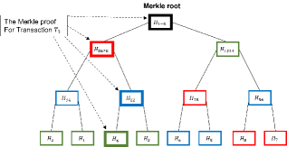
Figure 4: Illustration of a (colored) swapped Merkle tree, in which sibling nodes, e.g., $H_{1234}$ and $H_{5678}$, have been swapped. A Merkle proof in the ordinary Merkle tree (see Fig. 1) corresponds to a root-to-leaf path in the swapped Merkled tree. Thanks to the Ancestral Property, each root-to-leaf path (ignoring the root) contains exactly one node for each color, which implies that PIR schemes can be simultaneously applied to different color classes without revealing the path.

II-C Private Information Retrieval

Private Information Retrieval (PIR) was first introduced by Chor-Goldreich-Kushilevitz-Sudan [12] and has since become an important area in data privacy. In a PIR scheme, one or more servers store a database of $n$ data items $\{x_{1},x_{2},\ldots,x_{N}\}$ while a client wishes to retrieve an item $x_{j}$ without revealing the index $j$ to the server(s). Depending on the way the privacy is defined, we have information-theoretic PIR (IT-PIR) or computational PIR (cPIR).

In an IT-PIR scheme, the database is often replicated among $k>1$ servers, and the client can retrieve $x_{j}$ without leaking any information about $j$ to any $t<k$ servers. In other words, to an arbitrary set of colluding $t$ servers, based on their requests received from the client, any $j$ is equally possible. The simplest two-server IT-PIR was introduced in [12] and works as follows. The two servers both store $x_{1},x_{2},\ldots,x_{N}$, where $x_{i}\in\mathbb{F}$, $i=1,2,\ldots,N$, and $\mathbb{F}$ is a finite field of characteristic two. To privately retrieve $x_{j}$, the client picks a random set $I\subseteq\{1,2,\ldots,N\}$ and requests $\sum_{i\in I}x_{i}$ from Server 1 and $x_{j}+\big{(}\sum_{i\in I}x_{i}\big{)}$ from Server 2. As $\mathbb{F}$ has characteristic two, $x_{j}$ can be extracted by adding the two answers. Also, as $I$ is a random set, from the query, each server, even with unlimited computational power, achieves no information about $j$.

By contrast, in a cPIR scheme (originally proposed by Kushilevitz-Ostrovsky [13]), only one server is required and the privacy of the retrieved item $x_{j}$ relies on the hardness of a computational problem. Assuming that the server doesn’t have unlimited computational power, breaking the privacy is hard to achieve. While IT-PIR schemes generally have lower computation costs than their cPIR counterparts, the restriction on the maximum number of colluding servers is theoretically acceptable but hard to be enforced in practice, making them less desirable in real-world applications. Some recent noticeable practical developments (theory and implementation) include SealPIR [18, 38], which is based on Microsoft SEAL (Simple Encrypted Arithmetic Library) [38], and MulPIR from a Google research team [41].

II-D Batch Private Information Retrieval

We define below a computational batch-PIR scheme. The information-theoretic version can be defined similarly. The problem of privately retrieving a Merkle proof from a Merkle tree can be treated as a special case of the batch-PIR problem: the tree nodes form the database and the proof forms a batch.

Definition 1 (batch-PIR).

A (single-server) $(n,h)$ batch-PIR protocol consists of three algorithms described as follows.

• $\bm{q}\leftarrow\mathcal{Q}(n,1^{\lambda},B)$ is a randomized query-generation algorithm for the client. It takes as input the database size $n$, the security parameter $\lambda$, and a set $B\subseteq[n]$, $|B|=h$, and outputs the query $\bm{q}$.

• $\bm{a}\leftarrow\mathcal{A}(\bm{x},1^{\lambda},\bm{q})$ is a deterministic algorithm used by the server, which takes as input the database $\bm{x}$, the security parameter $\lambda$, the query $\bm{q}$, and outputs the answer $\bm{a}$.

• $\{x_{i}\}_{i\in B}\leftarrow\mathcal{R}(1^{\lambda},B,\bm{a})$ is a deterministic algorithm run by the client, which takes as input the security parameter $\lambda$, the index set $B$, the answer $\bm{a}$ from the server, and reconstructs $\{x_{i}\}_{i\in B}$.

Definition 2 (Correctness).

A batch-PIR protocol is correct if the client is always able to successfully retrieve $\{x_{i}\}_{i\in B}$ from the answer given that all parties correctly follow the protocol.

We denote by $\lambda\in\mathbb{N}$ the security parameter, e.g. $\lambda=128$, and ${\sf{negl}}(\lambda)$ the set of negligible functions in $\lambda$. A positive-valued function $\varepsilon(\lambda)$ belongs to ${\sf{negl}}(\lambda)$ if for every $c>0$, there exists a $\lambda_{0}\in\mathbb{N}$ such that $\varepsilon(\lambda)<1/\lambda^{c}$ for all $\lambda>\lambda_{0}$.

Definition 3 (Computational Privacy).

The privacy of a PIR protocol requires that a computationally bounded server cannot distinguish, with a non-negligible probability, between the distributions of any two queries $\bm{q}(B)$ and $\bm{q}(B^{\prime})$. More formally, for every database $\bm{x}$ of size $n$, for every $B,B^{\prime}\subset[n]$, $|B|=|B^{\prime}|=h$, and for every probabilistic polynomial time (PPT) algorithm $\mathfrak{A}$, it is required that

$$|\Pr[\bm{q}(B)\overset{R}{\leftarrow}\mathcal{Q}(n,1^{\lambda},B)\colon\mathfrak{A}(n,h,1^{\lambda},\bm{q}(B))=1]-\\ \Pr[\bm{q}(B^{\prime})\overset{R}{\leftarrow}\mathcal{Q}(n,1^{\lambda},B^{\prime})\colon\mathfrak{A}(n,h,1^{\lambda},\bm{q}(B^{\prime}))=1]|\in{\sf{negl}}(\lambda).$$

Note that our approach to batch-PIR, which is similar to most related work, e.g. [18, 42], simply splits the database into independent sub-databases and applies an existing PIR on each. Therefore, the privacy of our constructed batch-PIR reduces to that of the underlying PIR scheme in a straightforward manner. To speed up the server-side computation, we assume a single server that runs multi threads or multiple (all-colluding) servers that handle a batch request simultaneously.

III Parallel Private Retrieval of Merkle Proofs via Tree Colorings

In this section, we first describe the problem of parallel private retrieval of Merkle proofs and then propose an efficient solution that is based on the novel concept of tree coloring (Algorithm 1). We also introduce a fast algorithm with no communication overhead to resolve the sub-index problem: after partitioning a height-$h$ tree into $h$ sets of nodes $C_{1},C_{2},\ldots,C_{h}$, one must be able to quickly determine the sub-index of an arbitrary node $j$ in $C_{i}$, for every $i=1,2,\ldots,h$. We note that existing solutions to this problem often require the client to perform $\mathcal{O}(N)$ operations, where $N$ is the number of nodes in the tree. Our algorithm only requires the client to perform $\mathcal{O}(h^{3})=\mathcal{O}\big{(}(\log N)^{3}\big{)}$ operations. Finally, we provide detailed descriptions and a theoretical comparison of our work and existing schemes in the literature.

III-A Problem Description

Given a (perfect) Merkle tree stored at one or more servers, we are interested in designing an efficient private retrieval scheme in which a client can send queries to the server(s) and retrieve an arbitrary Merkle proof without letting the server(s) know which proof is being retrieved. As discussed in the Introduction and Section II-B, this problem is equivalent to the problem of designing an efficient private retrieval scheme for every root-to-leaf path in a perfect binary tree (with height $h$ and $n=2^{h}$ leaves). An efficient retrieval scheme should have low storage, computation, and communication overheads. The server(s) should not be able to learn which path is being retrieved based on the queries received from the client. The problem can be stated as a batch PIR problem (Definition 1), where the tree nodes form the database and the batch corresponds to the set of nodes in the Merkle proof.

We assume a setting in which the nodes of a Merkle/perfect binary tree are stored at one multi-core server or multiple (single-core) servers. Hence, the system is capable of parallel processing (see also the discussion after Definition 3). This assumption, which is relevant to Bitcoin and similar blockchains where the Merkle tree is replicated (as the main part of a block) in all full nodes, is essential for our approach to work. For brevity, we use the multi-server setting henceforth. To simplify the discussion, we assume that the servers have the same storage/computational capacities, and that they will complete the same workload in the same duration of time.

III-B Coloring/Partitioning-Based Parallel Private Retrieval of Merkle Proofs

To motivate our approach, we first describe a trivial private retrieval scheme using any existing PIR scheme in an obvious manner as follows. Suppose each of the $h$ servers stores the entire Merkle tree. The client can simply run the same PIR scheme on the $h$ servers in parallel, retrieving privately one node of the Merkle proof from each. We refer to this trivial solution as the $h$-Repetition scheme. Let $N$ be the total number of nodes (excluding the root) in a (perfect) Merkle tree of height $h$, then $N=2^{h+1}-2$. Suppose the PIR scheme requires ${\mathsf{C}}(N)$ operations on an $N$-item database, then every server needs to perform ${\mathsf{C}}(N)$ operations in the $h$-Repetition scheme. Our main observation is that each server only needs to perform PIR operations on a part of the tree instead of the whole tree, hence saving the storage and computational overheads.

Our proposal is to partition the (swapped) Merkle tree into $h$ balanced (disjoint) parts (sub-databases) of sizes $\lfloor N/h\rfloor$ or $\lceil N/h\rceil$, and let $h$ servers run the same PIR scheme on these $h$ parts in parallel (see Fig. 6). Note that partitioning the tree into $h$ parts is equivalent to coloring its nodes with $h$ colors: two nodes have the same colors if any only if they belong to the same part. Compared to the $h$-Repetition scheme, each server now runs on a smaller PIR sub-database and needs at most $C(\lceil N/h\rceil)$ operations to complete its corresponding PIR, speeding up the computation by a factor of $h$.

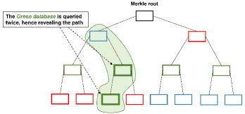
Figure 5: Example of a “bad” partition of the swapped Merkle tree, which partitions the tree into three sub-databases, corresponding to three different colors Red, Green, and Blue. The Merkle proof corresponding to the third leaf is a root-to-leaf path from this leaf, which contains two green nodes. As a consequence, the client needs to query the server storing the green sub-database twice, revealing the path. Note that all other root-to-leaf paths contain exactly one node of each color.

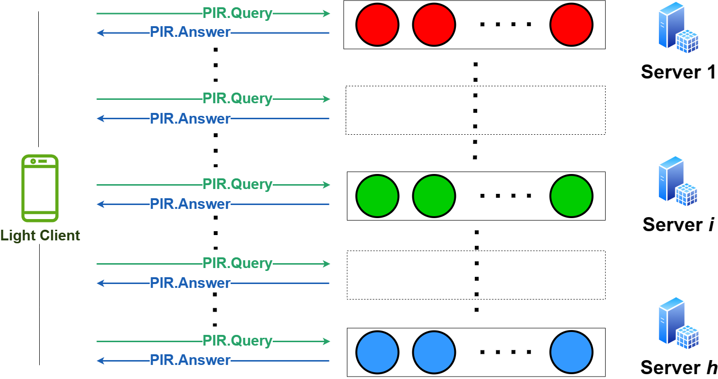
Figure 6: An illustration of our coloring-based parallel private retrieval of Merkle proofs. First, the nodes of the Merkle tree of height $h$ are partitioned into $h$ parts/color classes/sub-databases, each of which is stored by a server. The client runs $h$ PIR schemes with these $h$ servers in parallel to privately retrieve $h$ nodes of the Merkle proof, one from each server. Here, PIR.Query and PIR.Answer refers to the query and answer generations in the PIR scheme.

However, as demonstrated in Fig. 2 in the Introduction, not every tree partition preserves privacy. We reproduce this example for the swapped Merkle tree in Fig. 5. The reason this partition breaks the privacy, i.e., revealing the retrieved path even though the underlying PIR scheme by itself doesn’t reveal which nodes are being retrieved, is because the color patterns of different parts are not identical. More specifically, the root-to-the-third-leaf path (excluding the root) has one blue and two green nodes, while the rest have one red, one blue, and one green nodes. As the path corresponding to the third leaf has a distinctive color pattern, the “green” server can tell if the retrieved path corresponds to this leaf or not. This observation motivates the concept of ancestral colorings of rooted trees defined below, which requires that the nodes along every root-to-leaf path must have different colors. For a perfect binary tree, this condition corresponds precisely to the property that all root-to-leaf paths have identical color patterns.

Definition 4 (Ancestral Coloring).

A (node) coloring of a rooted tree of height $h$ using $h$ colors $1,2,\ldots,h$ is referred to as an ancestral coloring if it satisfies the Ancestral Property defined as follows.

• (Ancestral Property) Each color class $C_{i}$, which consists of tree nodes with color $i$, doesn’t contain any pair of nodes $u$ and $v$ so that $u$ is an ancestor of $v$. In other words, nodes that have ancestor-descendant relationship must have different colors.

An ancestral coloring is called balanced if it also satisfies the Balanced Property defined below.

• (Balanced Property) $\left||C_{i}|-|C_{j}|\right|\leq 1$, $\forall i,j\leq h$.

As previously mentioned, a trivial ancestral coloring is the coloring by layers, i.e., for a perfect binary tree, $C_{1}=\{2,3\}$, $C_{2}=\{4,5,6,7\}$, etc. The layer-based coloring, however, is not balanced. In Section IV, we will present a near-linear-time divide-and-conquer algorithm that finds a balanced ancestral coloring for every perfect binary tree. In fact, our algorithm is capable of finding an ancestral coloring for every feasible color sequences $(c_{1},c_{2},\ldots,c_{h})$, where $c_{i}$ denotes the number of tree nodes having color $i$, not just the balanced ones. This generalization can be used to accommodate the case when servers have heterogeneous storage/computational capacities.

Our coloring-based parallel private retrieval scheme of Merkle proofs is presented in Algorithm 1. Note that the pre-processing step is performed once per Merkle tree/database and can be done offline. The time complexity of this step is dominated by the construction of a balanced ancestral coloring, which is $\mathcal{O}(N\log\log(N))=O\big{(}2^{h}\log(h)\big{)}$. In fact, the ancestral coloring can be generated once and used for all (perfect) Merkle trees of the same height, regardless of the contents stored it their nodes. Nodes in the tree are indexed by $1,2,\ldots,N+1$ in a top-down left-right manner, where $1$ is the index of the root.

1:  Input: A Merkle tree, tree height $h$, and a leaf index $j$;   //Pre-processing: // Performed offline once per Merkle tree/database

2:  Generate the swapped Merkle tree $T(h)$;

3:  Find a balanced ancestral coloring $\{C_{i}\}_{i=1}^{h}$ for $T(h)$;

4:  Server $i$ stores tree nodes $\mathcal{T}_{i}$ indexed by $C_{i}$, $i=1,\ldots,h$;   //Parallel PIR: // Run the same PIR scheme on $h$ servers

5:  The client finds the indices $k_{1},\ldots,k_{h}$ of the nodes in the root-to-leaf-$j$ path by setting $k_{h}:=j$ and $k_{\ell}:=\lfloor k_{\ell+1}/2\rfloor$ for $\ell=h-1,h-2,\ldots,1$;

6:  The client finds the index $j_{k_{\ell}}$ of the node $k_{\ell}$ in its corresponding color class $C_{i_{\ell}}$, for $\ell=1,2,\ldots,h$; // which takes time $\mathcal{O}(h^{3})$, see the indexing Algorithm 3 and Theorem 3

7:  for $\ell=1$ to $h$ do

8:     The client and Server $i_{\ell}$ run (in parallel) a PIR scheme to retrieve node indexed $j_{k_{\ell}}$ from the sub-database $\mathcal{T}_{i_{\ell}}$;

9:  end for

10:  The client uses $h$ retrieved nodes to form the Merkle proof;

Algorithm 1 Coloring-Based Parallel Private Retrieval of Merkle Proofs

As an example, taking the tree of height $h=3$ depicted in Fig. 3, our algorithm first finds a balanced ancestral coloring $C_{1}=\{2,6,14,15\}$, $C_{2}=\{8,9,10,11,3\}$, and $C_{3}=\{4,5,12,13,7\}$ (line 3). Note how the elements in each $C_{i}$ are listed using a left-to-right order, that is, the elements on the left are listed first, and not a natural increasing order. This order guarantees a fast indexing in a later step. Next, suppose that the client wants to retrieve all the nodes in the root-to-leaf-$11$ path, i.e., $j=11$. The client can determine the indices of these nodes in $h=3$ steps: $k_{3}=j=11$, $k_{2}=\lfloor 11/2\rfloor=5$, and $k_{1}=\lfloor 5/2\rfloor=2$ (line 5). It then uses Algorithm 3 (see Section IV-C and the discussion below) to determine the index of each node in the corresponding color class, namely, node $k_{1}=2$ is the first node in $C_{1}$ ($j_{k_{1}}=1$), node $k_{2}=5$ is the second node in $C_{3}$ ($j_{k_{2}}=2$), and node $k_{3}=11$ is the fourth node in $C_{2}$ ($j_{k_{3}}=4$) (line 6). Finally, knowing all the indices of these nodes in their corresponding color classes/databases, the client sends one PIR query to each database to retrieve privately all nodes in the desired root-to-leaf path (lines 7-10).

The sub-index problem and existing solutions. For the client to run a PIR scheme on a sub-database, it must be able to determine the sub-index $j_{k_{\ell}}$ of each node $k_{\ell}$ in $C_{i_{\ell}}$, $\ell=1,\ldots,h$ (line 6 of Algorithm 1). We refer to this as the sub-index problem. Before describing our efficient approach to solve this problem, which requires no communication between servers and client and only requires $\mathcal{O}(h^{3})$ space and time, we discuss some relevant solutions suggested in the literature.

For brevity, we use below $i$, $k$, and $j_{k}$, instead of $i_{\ell}$, $k_{\ell}$, and $j_{k_{\ell}}$. Angel et al. [18, 43] proposed three approaches to solve the sub-index problem in the context of their probabilistic batch code (see Section III-C for a description), two of which are applicable in our setting. These solutions were also used in the most recent related work by Mughees and Ren [42]. Their first solution requires the client to download a Bloom filter [44] from each server. The Bloom filter $B_{i}$, which corresponds to $C_{i}$, stores the pairs $(k,j_{k})$ for all $k\in C_{i}$, where $j_{k}$ is the corresponding index of $k$ in $C_{i}$. Using $B_{i}$, the client can figure out $j_{k}$ for each $k$ by testing sequentially all pairs $(k,j^{\prime})$ for $j^{\prime}=1,2,\ldots,|C_{i}|$ against the filter. The main drawback of this approach is that in the average and worst cases, $\Theta(|C_{i}|)=\Theta(N/h)$ tests are required before the right index $j_{k}$ can be found. Furthermore, a larger Bloom filter must be sent to the client to keep the false positive probability low. Their second solution is to let the client rerun the item-to-database allocation (a process similar to our node-to-color assignment), which also takes $\Theta(N)$ steps given $N$ items. Both approaches are not scalable and becomes quite expensive when the database size reaches millions to billions items. Another way to solve the sub-index problem is to apply a private index retrieval scheme, which is, according to our experiment, more computationally efficient compared to the Bloom filter approach, but still incurs significant running time. We discuss this approach in detail in Appendix A.

An efficient solution to the sub-index problem with space/time complexity $\mathcal{O}(h^{3})$ and zero communication overhead. In Algorithm 3, which is described in detail later in Section IV-C, we develop an efficient approach to solve the sub-index problem. In essence, Algorithm 3 relies on a miniature version of our main Color-Splitting Algorithm (CSA) (see Section IV), which finds an ancestral coloring for a perfect binary tree. Instead of rerunning the algorithm on the whole tree (which requires $\mathcal{O}(N)$ operations), it turns out that the client can just run the algorithm on the nodes along a root-to-leaf path, which keeps the computation cost in the order of $\mathcal{O}(h^{3})=\mathcal{O}\big{(}(\log N)^{3}\big{)}$ instead of $\mathcal{O}(N)$. By keeping track of the number of nodes of colors $i=1,2,\ldots,h$ on the left of each node along this path, the algorithm can easily calculate the sub-index of the unique node of color $i$ within $C_{i}$ in this path. More details can be found in Section IV-C.

Assuming the parallel setting (e.g. multi-server), we define the (parallel) server time as the maximum time that a server requires to complete the task of interest, e.g., PIR processing (generating answers to queries). Theorem 1 summarizes the discussion so far on the privacy and the reduction in server storage overhead and computational complexity of our coloring-based approach (Algorithm 1). In particular, our scheme incurs no redundancy in storage on the server side as opposed to most related works (see Section III-C). Additionally, the server time is reduced by a factor of $h$ thanks to the tree partition compared to the $h$-Repetition approach, which applies the same PIR scheme $h$ times to the tree.

Theorem 1.

Suppose that the underlying PIR scheme used in Algorithm 1 has the server time complexity ${\mathsf{C}}(d)$, where $d$ is the size of the PIR database. Assuming a multi-server setting, and the Merkle tree is perfect with height $h\in{\sf{poly}}(\lambda)$, the following statements about Algorithm 1 hold.

1. The partition of the tree database into sub-databases according to an ancestral coloring doesn’t break the privacy of individual PIR scheme. In other words, the servers cannot distinguish between different batch requests with a non-negligible probability.

2. The $h$ PIR sub-databases correspond to the color classes of the balanced ancestral coloring and have size $\lfloor N/h\rfloor$ or $\lceil N/h\rceil$ each, where $N=2^{h+1}-2$.

3. The parallel server time (excluding the one-time pre-processing step) is ${\mathsf{C}}(\lceil N/h\rceil)$.

Proof.

The last two statements are straightforward by the definition of a balanced ancestral coloring and the description of Algorithm 1. We show below that the first statement holds.

In Algorithm 1, the nodes in the input Merkle tree are first swapped with their siblings to generate the swapped Merkle tree. The Merkle proofs in the original tree correspond precisely to the root-to-leaf paths in the swapped tree. An ancestral coloring ensures that $h$ nodes along every root-to-leaf path (excluding the colorless root) have different colors. Equivalently, every root-to-leaf path has identical color pattern $[1,1,\ldots,1]$, i.e. each color appears exactly once. This means that to retrieve a Merkle proof, the client sends exactly one PIR query to each sub-database/color class. Hence, no information regarding the topology of the nodes in the Merkle proof is leaked as the result of the tree partition to any server. Thus, the privacy of the retrieval of the Merkle proof reduces to the privacy of each individual PIR scheme.

More formally, in the language of batch-PIR, as the client sends $h$ independent PIR queries $\bm{q}_{1},\ldots,\bm{q}_{h}$ to $h$ disjoint databases indexed by $C_{1},\ldots,C_{h}$ (as the color classes do not overlap), a PPT adversary cannot distinguish between queries $\bm{q}(B)$ for $B=\{k_{1},\ldots,k_{h}\}$ and queries $\bm{q}(B^{\prime})$ for $B^{\prime}=\{k^{\prime}_{1},\ldots,k^{\prime}_{h}\}$. More specifically, for every collection of $h+1$ PPT algorithms $\mathfrak{A},\mathfrak{A}_{1},\ldots,\mathfrak{A}_{h}$,

$$\begin{split}&\big{|}\Pr[\bm{q}(B)\overset{R}{\leftarrow}\mathcal{Q}(n,1^{\lambda},B)\colon\mathfrak{A}(n,h,1^{\lambda},\bm{q}(B))=1]\\ &-\Pr[\bm{q}(B^{\prime})\overset{R}{\leftarrow}\mathcal{Q}(n,1^{\lambda},B^{\prime})\colon\mathfrak{A}(n,h,1^{\lambda},\bm{q}(B^{\prime}))=1]\big{|}\\ &\leq\sum_{i=1}^{h}\bigg{(}\big{|}\Pr[\bm{q}(\{k_{i}\})\overset{R}{\leftarrow}\mathcal{Q}(n,1^{\lambda},\{k_{i}\})\colon\mathfrak{A}_{i}(n,h,1^{\lambda},\bm{q}(\{k_{i}\}))=1]\\ &-\Pr[\bm{q}(\{k^{\prime}_{i}\})\overset{R}{\leftarrow}\mathcal{Q}(n,1^{\lambda},\{k^{\prime}_{i}\})\colon\mathfrak{A}_{i}(n,h,1^{\lambda},\bm{q}(\{k^{\prime}_{i}\}))=1]\big{|}\bigg{)}\\ &\in{\sf{negl}}(\lambda),\end{split}$$

as each term in the last sum belongs to ${\sf{negl}}(\lambda)$ due to the privacy of the underlying PIR (retrieving a single element) and there are $h\in{\sf{poly}}(\lambda)$ terms only. ∎

Remark 1.

Apart from the obvious $h$-Repetition, another trivial approach to generate a parallel retrieval scheme is to use a layer-based ancestral coloring, in which $h$ PIR schemes are run in parallel on $h$ layers of the tree to retrieve one node from each layer privately. The computation time is dominated by the PIR scheme running on the bottom layer, which contains $2^{h}\approx N/2$ nodes. Compared to our proposed scheme, which is based on a balanced ancestral coloring of size $N/h$, the layer-based scheme’s server time is $h/2$ times longer.

III-C Related Works and Performance Comparisons

Approaches	Batch code	Batch-optimization
Subcube Code [45]	$\checkmark$
Combinatorial [46]	$\checkmark$
Balbuena Graphs [47]	$\checkmark$
Pung hybrid [48]	$\checkmark$
Probabilistic Batch Code [18]	$\checkmark$
Lueks and Goldberg [10]		$\checkmark$
Vectorized Batch PIR [42]	$\checkmark$	$\checkmark$
Our work	$\checkmark$

TABLE I: Two main approaches for constructing batch PIR and the corresponding grouping of existing works. Most works use batch codes while a few others propose optimization techniques to reduce the overhead when dealing with a batch.

Approaches	Total storage ($S$)	Number of databases (cores/servers/buckets)	Probability of failure	(Parallel) server time	Client time
Subcube Code [45]	$Nh^{\log_{2}\frac{\ell+1}{\ell}}$	$h^{\log_{2}{(\ell+1)}}$	$0$	$\mathcal{O}\big{(}\frac{N}{h^{\log_{2}\ell}}\big{)}$	$\mathcal{O}\big{(}Nh^{\log_{2}\frac{\ell+1}{\ell}}\big{)}$
Balbuena Graphs [47]	$2N$	$2(h^{3}-h)$	$0$	$\mathcal{O}\big{(}\frac{N}{h^{3}-h}\big{)}$	$\mathcal{O}(2N)$
Combinatorial Batch Code [46, Thm. 2.7]	$hN-(h-1){m\choose{h-1}}$	$m$ $\big{(}\text{for }{m\choose{h-1}}\leq\frac{N}{h-1}\big{)}$	$0$	$\mathcal{O}\bigg{(}\frac{hN}{m}-\frac{{{m-1}\choose{h-2}}}{m-h+1}\bigg{)}$	$\mathcal{O}\big{(}hN-(h-1){m\choose{h-1}}\big{)}$
SealPIR+PBC [18]	$3N$	$1.5h$	$2^{-20}$	$\mathcal{O}\big{(}\frac{2N}{h}\big{)}$	$\mathcal{O}(3N)$
SealPIR+Coloring	$N$	$h$	$0$	$\mathcal{O}\big{(}\frac{N}{h}\big{)}$	$\mathcal{O}(N)$
Lueks-Goldberg [10]	$N$	$1$	$0$	$\mathcal{O}\big{(}h^{0.80735}N\big{)}$	$\mathcal{O}\big{(}h\sqrt{N}\big{)}$
Vectorized BPIR [42]	$3N$	$1.5h$	$2^{-20}$	$\mathcal{O}\big{(}\frac{2N}{h}\big{)}$	$\mathcal{O}(4.5\sqrt[3]{2h^{2}N})$
Vectorized BPIR +Coloring	$N$	$h$	$0$	$\mathcal{O}\big{(}\frac{N}{h}\big{)}$	$\mathcal{O}(3\sqrt[3]{h^{2}N})$

TABLE II: A comparison of our scheme and related batch PIR schemes regarding the total storage overhead, the number $m$ of databases (or cores/servers/buckets), the server/client running times, and the failure probability. Here, $N$ and $h$ denote the number of tree nodes and the tree height, respectively, and $\ell\geq 2$ is the tuning parameter in the subcube code. The client’s time is much lower than the server’s time in practice as it only processes the indices. The big-O notation cannot capture this fact.

The problem of private retrieval of Merkle proofs can be treated as a special case of the batch PIR (BPIR) problem, in which an arbitrary subset of items instead of a single one needs to be retrieved. As a Merkle proof consists of $h$ nodes, the batch size is $h$. Thus, existing BPIR schemes can be used to solve this problem. However, a Merkle proof does not contain an arbitrary set of $h$ nodes like in the batch PIR’s setting. Indeed, there are only $n=2^{h}$ such proofs compared to $\binom{2n-2}{h}$ subsets of random $h$ nodes in the Merkle tree. We exploit this fact to optimize the storage overhead of our scheme compared to similar approaches using batch codes [45, 18, 42]. In this section, we conduct a review of existing works dealing with BPIR and a comparison with our coloring-based solution. Apart from having the optimal storage overhead, our coloring method can also be applied on top of some existing schemes such as those in [10, 42] and improve their performance.

There are two main approaches proposed in the literature to construct a BPIR scheme: the batch-code-based approach and the batch-optimization approach. We group existing works into these two categories in Table I. Our proposal belongs to the first category. However, as opposed to all existing batch-code-based schemes, ours incurs no storage redundancy. This is possible thanks to the special structure of the Merkle proofs and the existence of balanced ancestral colorings.

Batch codes, which were introduced by Ishai-Kushilevitz-Ostrovsky-Sahai [45], encode a database into $m$ databases (or buckets) and store them at $m$ servers in a way that allows a client to retrieve any batch of $h$ items by downloading at most one item from each server. A batch code can be used to construct a BPIR scheme. For example, in the so-called $(N,\frac{3N}{2},2,3)$ subcube code, a database $X=\{x_{i}\}_{i=1}^{N}$ is transformed into three databases: $X_{1}=\{x_{i}\}_{i=1}^{N/2}$, $X_{2}=\{x_{i}\}_{i={N/2}+1}^{N}$, and $X_{3}=X_{1}\bigoplus X_{2}=\{x_{i}\oplus x_{i+{N/2}}\}_{i=1}^{N/2}$. Assume the client wants to privately retrieve two items $x_{j_{1}}$ and $x_{j_{2}}$. If $x_{j_{1}}$ and $x_{j_{2}}$ belong to different databases then the client can send two PIR queries to these two databases for these items, and another to retrieve a random item in the third database. If $x_{j_{1}}$ and $x_{j_{2}}$ belong to the same sub-database, for example, $X_{1}$, then the client will send three parallel PIR queries to retrieve $x_{j_{1}}$ from $X_{1}$, $x_{j_{2}+N/2}$ from $X_{2}$, and $x_{j_{2}}\oplus x_{j_{2}+N/2}$ from $X_{3}$. The last two items can be XOR-ing to recover $x_{j_{2}}$. More generally, by recursively applying the construction, the subcube code [45] has a total storage of $Nh^{\log_{2}\frac{\ell+1}{\ell}}$ with $m=h^{\log_{2}{(\ell+1)}}$ databases/servers. Tuning the parameter $\ell\geq 2$ provides a trade-off between the storage overhead and the number of servers required. Another example of batch codes was the one developed in [47], which was based on small regular bipartite graph with no cycles of length less than eight originally introduced by Balbuena [49].

Combinatorial batch codes (CBC), introduced by Stinson-Wei-Paterson [46], are special batch codes in which each database/bucket stores subsets of items (so, no encoding is allowed as in the subcube code). Our ancestral coloring can be considered as a relaxed CBC that allows the retrieval of not every but some subsets of $h$ items (corresponding to the Merkle proofs). By exploiting this relaxation, our scheme only stores $N$ items across all $h$ databases/buckets (no redundancy). By contrast, an optimal CBC, with $h$ databases/buckets, requires $\mathcal{O}(hN)$ total storage (see [46, Thm. 2.2], or [46, Thm. 2.7] with $m=h$). We also record this fact in Table II.

Probabilistic batch codes (PBC), introduced by Angel-Chen-Laine-Setty [18], is a probabilistic relaxation of CBC that offers a better trade-off between the total storage overhead and the number of servers/buckets required. A PBC can also be combined with an arbitrary PIR scheme to create a batch PIR. More specifically, a PBC uses $w$ independent hash functions $h_{1},\ldots,h_{w}$ to distribute items $i$ in the original database to $w$ among $m$ databases/buckets using the indices $h_{1}(i),\ldots,h_{w}(i)$. Hence, the total storage overhead is $wN$. In a typical setting, $w=3$ and $m=1.5h$ (ignoring the rounding). In comparison, for the setting of Merkle proof retrieval from a Merkle tree of height $h$ with $N=2^{h+1}-2$ nodes (excluding the root), a PBC uses $1.5h$ databases of size roughly $2N/h$ each, while our coloring-based scheme uses $h$ databases of size roughly $N/h$ each, leading to $3\times$ smaller storage overheads and $2\times$ faster running times (Table II). The retrieval uses the idea of Cuckoo hashing [50] to find a 1-to-1 matching/mapping between the $h$ items to be retrieved and the databases/buckets. The client then sends one PIR query to each server storing a matched database to retrieve the corresponding item. To preserve privacy, it also sends a PIR query for a dummy item from each of the remaining unmatched databases. As it is probabilistic, the retrieval of a subset of $h$ items may fail with a small probability $p$. This happens when the Cuckoo hashing fails to find a 1-to-1 matching between the $h$ items and the $m$ databases for the client. For the batch size $h<200$, which is the case for typical Merkle trees ($h$ is between 10 and 32), a PBC fails with probability $p\approx 2^{-20}$. The example in Fig. 7 illustrates a successful retrieval of the batch of items $\{6,8,9\}$, in which the Cuckoo hashing finds a mapping that maps this items to the second, the forth, and the fifth databases.

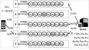
Figure 7: An illustration of a successful retrieval of a batch of items using a probabilistic batch code [18] with Cuckoo hashing [50] using three independent hash functions $h_{1},h_{2},h_{3}$. Five servers/cores can be used to process five databases in parallel.

The second approach, batch-optimization, aims to amortize the processing cost of a batch request [10, 42]. Lueks and Goldberg [10] combine the Strassen’s efficient matrix multiplication algorithm [51] and Goldberg’s IT-PIR scheme [26] to speed up the batch PIR process. In the one-client setting, the database with $N$ nodes is represented as a $\sqrt{N}\times\sqrt{N}$ matrix $D$. In the original PIR scheme [26], each server performs a vector-matrix multiplication of the query vector $q$ and the matrix $D$. In the batch PIR version, the $h$ PIR query vectors $q_{1},\ldots,q_{h}$ are first grouped together to create an $h\times\sqrt{N}$ query matrix $Q$. Each server then applies Strassen’s algorithm to perform the fast matrix multiplication $QD$ to generate the responses, incurring a computational complexity of $\mathcal{O}\big{(}h^{0.80735}N\big{)}$ (instead of $\mathcal{O}(hN)$ as in an ordinary matrix multiplication).

In the multi-client setting in which $c$ clients requests $c$ Merkle proofs (one per client), there are two possible approaches to implement Lueks-Goldberg’s strategy. In the first approach, the input database is still represented as a $\sqrt{N}\times\sqrt{N}$ matrix $D$ as before, and each client sends a batch of $h$ PIR-queries for one Merkle proof. In the second approach, a new proof-database is created, which contains $n=2^{h}$ Merkle proofs as items ($h$ hashes each). The proof-database corresponding to a Merkle tree with $n$ leaves can be represented by a $\sqrt{hn}\times\sqrt{hn}$ matrix $P$. Each client sends one PIR query to receive one item (one Merkle proof) from the servers. In both cases, the PIR queries are grouped together to create a query matrix $Q$ of size either $(ch)\times\sqrt{N}$ or $c\times\sqrt{hn}\approx c\times\sqrt{hN/2}$ for perfect trees, noting that $n\approx N/2$. Applying the Strassen’s algorithm to multiply $Q$ with $D$ or $P$, the number of operations required is either $\mathcal{O}\big{(}(ch)^{0.80735}N\big{)}$ or $\mathcal{O}\big{(}c^{0.80735}hN/2\big{)}$ (see Table III). Our ancestral coloring can be combined with Lueks-Goldberg’s schemes to improve their storage overhead and running time as follows. Using an ancestral coloring, we can partition the tree nodes into $h$ sub-databases $\mathcal{T}_{i}$ represented by $h$ $\sqrt{N/h}\times\sqrt{N/h}$ matrices, $1\leq i\leq h$. As Luke-Goldberg PIR scheme, although uses multiple servers, processes PIR queries in a sequential mode, to make a fair comparison, we also assume that in our coloring-based scheme each server processes all the $h$ sub-databases sequentially. Note that in our scheme, each of the $c$ clients will send $h$ PIR queries to $h$ sub-databases in each server. Each server then performs $h$ multiplications of a $c\times\sqrt{N/h}$ matrix and a $\sqrt{N/h}\times\sqrt{N/h}$ matrix, incurring a cost of $\mathcal{O}\big{(}c^{0.80735}N\big{)}$ operations, outperforming Luke-Goldberg’s schemes by at least a factor of $h^{0.80735}\times$.

	Lueks-Goldberg [10]		LG [10] + Coloring
Database	$\sqrt{N}\times\sqrt{N}$	$\sqrt{\frac{hN}{2}}\times\sqrt{\frac{hN}{2}}$	$h\left(\sqrt{\frac{N}{h}}\times\sqrt{\frac{N}{h}}\right)$
Multiplications	${(ch)}^{0.80735}N$	$c^{0.80735}\frac{hN}{2}$	$c^{0.80735}N$
Additions	$\frac{8}{3}{(ch)}^{0.80735}N$	$\frac{8}{3}c^{0.80735}\frac{hN}{2}$	$\frac{8}{3}{c}^{0.80735}N$

TABLE III: A comparison of Lueks-Goldberg’s IT-PIR schemes and a combination with our coloring regarding the number of server operations. In this setting, $c$ clients wants to receive $c$ Merkle proofs (one proof per client) privately.

The work of Kales, Omolola, and Ramacher [11] aimed particularly for the Certificate Transparency infrastructure and improved upon Lueks and Goldberg’s work [10] for the case of a single client with multiple queries over large dynamic Merkle trees with millions to billions leaves (certificates). Their idea is to split the original Merkle tree into multiple tiers of smaller trees with heights ranging from $10$ to $16$, where the trees at the bottom store all the certificates. The Merkle proofs for the certificates within each bottom tree (static, not changing over time) can be embedded inside a Signed Certificate Timestamp, which goes together with the certificate itself. These Merkle proofs can be used to verify the membership of the certificates within the bottom trees. The roots of these trees form the leaves of the (dynamic) top Merkle tree that changes over time as more certificates are appended to the tree. To verify that a certificate is actually included in the large tree, the client now only needs to send PIR query for the Merkle proof of the root of the bottom tree in the top tree. Note that the top tree is much smaller than the original one, e.g. a tree of height 30 can be organized into a top tree of height 15 and at most $2^{15}$ trees of height 15 at the bottom. A batch PIR scheme such as Lueks-Goldberg [10] can be used for the top tree.

The authors of [11] also proposed a more efficient alternative PIR scheme, which employs Distributed Point Functions (DPF) [52, 53, 54]. The client simply sends a PIR query to retrieve one hash in each level/layer of the top tree (same as the layer-based approach described in Remark 1). For two servers, thanks to the existence of DPF that uses queries of size $\mathcal{O}(\log N)$ only (with $N$ being the number of nodes in the dynamic tree), the corresponding PIR scheme runs very fast, achieving running times in milliseconds for both servers and client and small communication overheads. Although the scheme proposed by Kales, Omolola, and Ramacher [11] is very practical, we do not include it in the comparisons with other schemes in Table II. The reason is that this scheme was designed particularly for Certificate Transparency with a clever modification tailored to such a system, hence requiring extra design features outside of the scope of the retrieval problem that we are discussing (e.g. the ability to embed the Merkle proofs in the bottom trees inside the Signed Certificate Timestamps). Note that to apply the ancestral coloring to the dynamic tree in [11] (assumming multi-core servers), we will need to extend the theory of ancestral coloring to growing trees, which remains an intriguing question for future research.

The most recent batch-optimizing technique is Vectorized BPIR proposed by Mughees and Ren [42], which also uses probabilistic batch codes [18] but with a more batch-friendly vectorized homomorphic encryption. More specifically, instead of running independent PIR schemes for the databases/buckets, this scheme merges the queries from the client and the responses from the databases to reduce the communication overhead. By replacing the PBC component by our coloring, we can reduce the number of databases/buckets of Vectorized BPIR from $1.5h$ to $h$, and the database/bucket size by a factor of two, from $2N/h$ to $N/h$, hence optimizing its storage overhead and and reduce the server running time for the retrieval of Merkle proofs (see Table II). More details about Vectorized BPIR and how we can improve it using an ancestral coloring are presented below.

Just like SealPIR [18], a Vectorized BPIR [42] also uses a PBC to transform the original database of $N$ items into $m=1.5h$ databases/buckets, each containing roughly $N_{B}\approx 2N/h=3N/1.5h$ items (each item is replicated three times). Each database is then represented as a $d$-dimensional $N_{B}^{\prime}\times N_{B}^{\prime}\times\cdots\times N_{B}^{\prime}$ cube where $N_{B}^{\prime}=\sqrt[d]{N_{B}}$. The authors recommend to set $d=3$ for the best performance trade-off. The client sends $d=3$ queries to each database, all packed inside three ciphertexts across the databases (with respect to the somewhat homomorphic encryption (SHE) based on the Ring Learning with Errors (RLWE) problem). Each database processes the queries separately but at the end packs all the responses together inside a single ciphertext and sends back to the client. Note that this is possible, as observed in [42], because the ciphertext size is sufficiently large compared to the parameters of a practical PIR system. Here, the authors assume a single-server setting. Hence, in the parallel mode, we can assume that each database is handled by a different core of the server, but their outputs will be aggregated into a single ciphertext before being sent to the client. By contrast, SealPIR [18] requires at least two ciphertexts for the query and response for each database, resulting in a large communication overhead for batches of small items (as ciphertext is large).

With the received queries packed in ciphertexts and the stored data items represented as plaintexts, each database in Vectorized BPIR performs a number of ciphertext-plaintext multiplications (fastest, e.g. 0.09 ms per operation), ciphertext-ciphertext (slowest, e.g. 12.1 ms per operation), and ciphertext rotations (3.6 ms per operation) to produce the PIR responses (see [42] for more details). Setting $d=3$, the numbers of these operations are proportional to $N_{B}=2N/h$, $\sqrt[3]{N_{B}^{2}}+\sqrt[3]{N_{B}}$, and $2\sqrt[3]{N_{B}^{2}}+\sqrt[3]{N_{B}}(\log\sqrt[3]{N_{B}}-1)$, respectively. In Table II, we write $O(2N/h)$ to capture the scheme’s running time complexity. By replacing the PBC by an ancestral coloring, we can reduce the number of databases from $1.5h$ to $h$, and the size of each database from $N_{B}=2N/h$ to $N/h$, hence improving the storage and running time complexity. Moreover, the improved scheme can run without failures.

IV A Divide-And-Conquer Algorithm for Finding Ancestral Colorings of Perfect Binary Trees

IV-A The Color-Splitting Algorithm

As discussed in the previous section, our proposed parallel private retrieval scheme given in Algorithm 1 requires a balanced ancestral coloring of the Merkle tree. We develop in this section a divide-and-conquer algorithm that finds an ancestral coloring (if any) given an arbitrary color class sizes for a perfect binary tree in almost linear time. Note that even if we only want to find a balanced coloring, our algorithm still needs to handle unbalanced cases in the intermediate steps. First, we need the definition of a color sequence.

Definition 5 (Color sequence).

A color sequence of dimension $h$ is a sorted sequence of positive integers $c$, where $c_{1}\leq c_{2}\leq\cdots\leq c_{h}$. The sum $\sum_{i=1}^{h}c_{i}$ is referred to as the sequence’s total size. The element $c_{i}$ is called the color size, which represents the number of nodes in a tree that will be assigned Color $i$. The color sequence $\vec{c}$ is called balanced if the color sizes $c_{i}$ differ from each other by at most one, or equivalently, $c_{j}-c_{i}\leq 1$ for all $h\geq j>i\geq 1$. It is assumed that the total size of a color sequence is equal to the total number of nodes in a tree (excluding the root).

The Color-Splitting Algorithm (CSA) starts from a color sequence $\vec{c}$ and proceeds to color the tree nodes, two sibling nodes at a time, from the top of the tree down to the bottom in a recursive manner while keeping track of the number of remaining nodes that can be assigned Color $i$. Note that the elements of a color sequence $\vec{c}$ are always sorted in non-decreasing order, e.g., $\vec{c}=$ [4 Red, 5 Green, 5 Blue], and CSA always try to color all the children of the current root $R$ with either the same color $1$ if $c_{1}=2$, or with two different colors $1$ and $2$ if $2<c_{1}\leq c_{2}$. The intuition is to use colors of smaller sizes on the top layers and colors of larger sizes on the lower layers (more nodes). The remaining colors are split “evenly” between the left and the right subtrees of $R$ while ensuring that the color used for each root’s child will no longer be used for the subtree rooted at that node to guarantee the Ancestral Property. The key technical challenge is to make sure that the split is done in a way that prevents the algorithm from getting stuck, i.e., to make sure that it always has “enough” colors to produce ancestral colorings for both subtrees (a formal discussion is provided below). If a balanced ancestral coloring is required, CSA starts with the balanced color sequence $\vec{c}^{*}=[c^{*}_{1},\ldots,c^{*}_{h}]$, in which the color sizes $c^{*}_{i}$’s differ from each other by at most one.

Before introducing rigorous notations and providing a detailed algorithm description, let start with an example of how the algorithm works on $T(3)$.

Example 1.

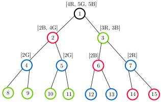
Figure 8: An illustration of the Color-Splitting Algorithm being applied to $T(3)$ and the initial color sequence $\vec{c}=[4,5,5]$. The feasible color sequences used at different node (regarded as root nodes of subtrees) are also given. The splits of color sequences follow the rule in the Procedure FeasibleSplit(), while the assignment of colors to nodes follow the Procedure ColorSplittingRecursive().

The Color-Splitting Algorithm starts from the root node 1 with the balanced color sequence $\vec{c}^{*}=[4,5,5]$, which means that it is going to assign Red (Color 1) to four nodes, Green (Color 2) to five nodes, and Blue (Color 3) to five nodes (see Fig. 8). We use $[4\text{R},5\text{G},5\text{B}]$ instead of $[4,5,5]$ to keep track of the colors. Note that the root needs no color. According to the algorithm’s rule, as Red and Green have the lowest sizes, which are greater than two, the algorithm colors the left child (Node 2) red and the right child (Node 3) green. The dimension-$3$ color sequence $\vec{c}=[4\text{R},5\text{G},5\text{B}]$ is then split into two dimension-$2$ color sequences $\vec{a}=[2\text{B},4\text{G}]$ and $\vec{b}=[3\text{R},3\text{B}]$. How the split works will be discussed in detail later, however, we can observe that both resulting color sequences have a valid total size $6=2+2^{2}$, which matches the number of nodes in each subtree. Moreover, as $\vec{a}$ has no Red and $\vec{b}$ has no Green, the Ancestral Property is guaranteed for Node 2 and Node 3, i.e., these two nodes have different colors from their descendants. The algorithm now repeats what it does to these two subtrees rooted at Node 2 and Node 3 using $\vec{a}$ and $\vec{b}$. For the left subtree rooted at 2, the color sequence $\vec{a}=[2\text{B},4\text{G}]$ has two Blues, and so, according to CSA’s rule, the two children 4 and 5 of 2 both receive Blue as their colors. The remaining four Greens are split evenly into $[2\text{G}]$ and $[2\text{G}]$, to be used to color $8,9,10$, and $11$. The remaining steps are carried out in the same manner.

We observe that not every color sequence $c$ of dimension $h$, even when having a valid total size $\sum_{i=1}^{h}c_{i}$, can be used to construct an ancestral coloring of the perfect binary tree $T(h)$. For example, it is easy to verify that there are no ancestral colorings of $T(2)$ using $\vec{c}=[1,5]$, i.e., 1 Red and 5 Greens, and similarly, no ancestral colorings of $T(3)$ using $\vec{c}=[2,3,9]$, i.e., 2 Reds, 3 Greens, and 9 Blues. It turns out that there is a very neat characterization of all color sequences of dimension $h$ for that an ancestral coloring of $T(h)$ exists. We refer to them as $h$-feasible color sequences (see Definition 6).

Definition 6 (Feasible color sequence).

A (sorted) color sequence $\vec{c}$ of dimension $h$ is called $h$-feasible if it satisfies the following two conditions:

• (C1) $\sum_{i=1}^{\ell}c_{i}\geq\sum_{i=1}^{\ell}2^{i}$, for every $1\leq\ell\leq h$, and

• (C2) $\sum_{i=1}^{h}c_{i}=\sum_{i=1}^{h}2^{i}=2^{h+1}-2$.

Condition (C1) means that Colors $1,2,\ldots,\ell$ are sufficient in numbers to color all nodes in Layers $1,2,\ldots,\ell$ of the perfect binary tree $T(h)$ (Layer $i$ has $2^{i}$ nodes). Condition (C2) states that the total size of $c$ is equal to the number of nodes in $T(h)$.

The biggest challenge we face in designing the CSA is to maintain feasible color sequences at every step of the algorithm.

Example 2.

The following color sequences (taken from the actual coloring of nodes in the trees $T(1),T(2),T(3)$ in Fig. 3) are feasible: $[2]$, $[3,3]$, and $[4,5,5]$. The sequences $[2,3]$ and $[3,4,6,17]$ are not feasible: $2+3<6=2+2^{2}$, $3+4+6<14=2+2^{2}+2^{3}$. Clearly, color sequences of the forms $[1,\ldots]$, $[2,2,\ldots,]$ or $[2,3,\ldots]$, or $[3,4,6,\ldots]$ are not feasible due to the violation of (C1).

Definition 7.

The perfect binary $T(h)$ is said to be ancestral $\vec{c}$-colorable, where $c$ is a color sequence, if there exists an ancestral coloring of $T(h)$ in which precisely $c_{i}$ nodes are assigned Color $i$, for all $i=1,\ldots,h$. Such a coloring is called an ancestral $\vec{c}$-coloring of $T(h)$.

The following lemma states that every ancestral coloring for $T(h)$ requires at least $h$ colors.

Lemma 1.

If the perfect binary tree $T(h)$ is ancestral $\vec{c}$-colorable, where $\vec{c}=[c_{1},\ldots,c_{h^{\prime}}]$, then $h^{\prime}\geq h$. Moreover, if $h^{\prime}=h$ then all $h$ colors must show up on nodes along any root-to-leaf path (except the root, which is colorless). Equivalently, nodes having the same color $i\in\{1,2,\ldots,h\}$ must collectively belong to $2^{h}$ different root-to-leaf paths.

Proof.

A root-to-leaf path contains exactly $h$ nodes except the root. Since these nodes are all ancestors and descendants of each other, they should have different colors. Thus, $h^{\prime}\geq h$. As $T(h)$ has precisely $2^{h}$ root-to-leaf paths, other conclusions follow trivially. ∎

Theorem 2 characterizes all color sequences of dimension $h$ that can be used to construct an ancestral coloring of $T(h)$. Note that the balanced color sequence that corresponds to a balanced ancestral coloring is only a special case among all such sequences.

Theorem 2 (Ancestral-Coloring Theorem for Perfect Binary Trees).

For every $h\geq 1$ and every color sequence $c$ of dimension $h$, the perfect binary tree $T(h)$ is ancestral $\vec{c}$-colorable if and only if $\vec{c}$ is $h$-feasible.

Proof.

The Color-Splitting Algorithm can be used to show that if $\vec{c}$ is $h$-feasible then $T(h)$ is ancestral $\vec{c}$-colorable. For the necessary condition, we show that if $T(h)$ is ancestral $\vec{c}$-colorable then $\vec{c}$ must be $h$-feasible. Indeed, for each $1\leq\ell\leq h$, in an ancestral $\vec{c}$-coloring of $T(h)$, the nodes having the same color $i$, $1\leq i\leq\ell$, should collectively belong to $2^{h}$ different root-to-leaf paths in the tree according to Lemma 1. Note that each node in Layer $i$, $i=1,2\ldots,h$, belongs to $2^{h-i}$ different paths. Therefore, collectively, nodes in Layers $1,2,\ldots,\ell$ belong to $\sum_{i=1}^{\ell}2^{i}\times 2^{h-i}=\ell 2^{h}$ root-to-leaf paths. We can see that each path is counted $\ell$ times in this calculation. Note that each node in Layer $i$ belongs to strictly more paths than each node in Layer $j$ if $i<j$. Therefore, if (C1) is violated, i.e., $\sum_{i=1}^{\ell}c_{i}<\sum_{i=1}^{\ell}2^{i}$, which implies that the number of nodes having colors $1,2\ldots,\ell$ is smaller than the total number of nodes in Layers $1,2,\ldots,\ell$, then the total number of paths (each can be counted more than once) that nodes having colors $1,2,\ldots,\ell$ belong to is strictly smaller than $\ell 2^{h}$. As a consequence, there exists a color $i\in\{1,2,\ldots,\ell\}$ such that nodes having this color collectively belong to fewer than $2^{h}$ paths, contradicting Lemma 1. ∎

Corollary 1.

A balanced ancestral coloring exists for the perfect binary tree $T(h)$ for every $h\geq 1$.

Proof.

This follows directly from Theorem 2, noting that a balanced color sequence of dimension $h$ is also $h$-feasible (see Corollary 2 proved in the next section). ∎

We now formally describe the Color-Splitting Algorithm. The algorithm starts at the root $R$ of $T(h)$ with an $h$-feasible color sequence $c$ (see ColorSplitting$(h,\vec{c})$) and then colors the two children $A$ and $B$ of the root as follows: these nodes receive the same Color 1 if $c_{1}=2$ or Color 1 and Color 2 if $c_{1}>2$. Next, the algorithm splits the remaining colors in $c$ (whose total size has already been reduced by two) into two $(h-1)$-feasible color sequences $\vec{a}$ and $\vec{b}$, which are subsequently used for the two subtrees $T(h-1)$ rooted at $A$ and $B$ (see ColorSplittingRecursive$(R,h,\vec{c})$). Note that the splitting rule (see FeasibleSplit$(h,\vec{c})$) ensures that if Color $i$ is used for a node then it will no longer be used in the subtree rooted at that node, hence guaranteeing the Ancestral Property. We prove in Section IV-B that it is always possible to split an $h$-feasible sequence into two new $(h-1)$-feasible sequences, which guarantees a successful termination if the input of the CSA is an $h$-feasible color sequence. The biggest hurdle in the proof stems from the fact that after being split, the two color sequences are sorted before use, which makes the feasibility analysis rather involved. We overcome this obstacle by introducing a partition technique in which the elements of the color sequence $\vec{c}$ are partitioned into groups of elements of equal values (called runs) and showing that the feasibility conditions hold first for the end-points and then for the middle-points of the runs (more details in Lemmas 4-5-6 and the preceding discussions).

Example 3.

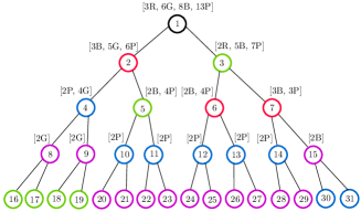
Figure 9: An illustration of the Color-Splitting Algorithm being applied to $T(4)$ and the initial color sequence $\vec{c}=[3,6,8,13]$. The feasible color sequences used at different nodes (regarded as root nodes of subtrees) are also given.

We illustrate the Color-Splitting Algorithm when $h=4$ in Fig. 9. The algorithm starts with a $4$-feasible sequence $\vec{c}=[3,6,8,13]$, corresponding to 3 Reds, 6 Greens, 8 Blues, and 13 Purples. The root node 1 is colorless. As $2<c_{1}=3<c_{2}=8$, CSA colors 2 with Red, 3 with Green, and splits $\vec{c}$ into $\vec{a}=[3\text{B},5\text{G},6\text{P}]$ and $\vec{b}=[2\text{R},5\text{B},7\text{P}]$, which are both $3$-feasible and will be used to color the subtrees rooted at 2 and 3, respectively. Note that $\vec{a}$ has no Red and $\vec{b}$ has no Green, which enforces the Ancestral Property for Node 2 and Node 3. The remaining nodes are colored in a similar manner.

Algorithm 2 ColorSplitting($h,\vec{c}$)

  // The algorithm finds an ancestral $\vec{c}$-coloring of $T(h)$

  Set $R:=1$; // the root of $T(h)$ is 1, which requires no color

  ColorSplittingRecursive$(R,h,\vec{c})$;

Procedure ColorSplittingRecursive$(R,h,\vec{c})$

1:  // This procedure colors the two children of $R$ and create feasible color sequences for its left and right subtrees. $R$ is the root node of the current subtree $T(h)$ of height $h$. Either $R$ needs no color ($R=1$) or $R$ has already been colored in the previous call. $c$ is a feasible color sequence ($2\leq c_{1}\leq c_{2}\leq\cdots\leq c_{h}$).

2:  if $h\geq 1$ then

3:     $A:=2R$; $B:=2R+1$; // left and right child of $R$

4:     if $c_{1}=2$ then

5:        Assign Color 1 to both $A$ and $B$;

6:     else

7:        Assign Color 1 to $A$ and Color 2 to $B$;

8:     end if

9:     if $h\geq 2$ then

10:        Let $\vec{a}$ and $\vec{b}$ be the output color sequences of FeasibleSplit$(h,\vec{c})$;

11:        ColorSplittingRecursive$(A,h-1,\vec{a})$;

12:        ColorSplittingRecursive$(B,h-1,\vec{b})$;

13:     end if

14:  end if

Procedure FeasibleSplit($h,\vec{c}$)

  // This algorithm splits a (sorted) $h$-feasible sequence into two (sorted) $(h-1)$-feasible ones, which will be used for coloring the subtrees, only works when $h\geq 2$

  // Case 1: $c_{1}=2$, note that $c_{1}\geq 2$ due to the feasibility of $\vec{c}$

  if $c_{1}=2$ then

     Set $a_{2}:=\lfloor c_{2}/2\rfloor$ and $b_{2}:=\lceil c_{2}/2\rceil$;

     Set $S_{2}(a):=a_{2}$ and $S_{2}(b):=b_{2}$; // $|S_{i}(a)-S_{i}(b)|\leq 1$ for $2\leq i\leq h$

     for $i=3$ to $h$ do

        if $S_{i-1}(a)<S_{i-1}(b)$ then

           Set $a_{i}:=\lceil c_{i}/2\rceil$ and $b_{i}:=\lfloor c_{i}/2\rfloor$;

        else

           Set $a_{i}:=\lfloor c_{i}/2\rfloor$ and $b_{i}:=\lceil c_{i}/2\rceil$;

        end if

        Update $S_{i}(a):=S_{i-1}(a)+a_{i}$ and $S_{i}(b):=S_{i-1}(b)+b_{i}$;

     end for

     //Case 2: $c_{1}>2$

  else

     Set $a_{2}:=c_{2}-1$ and $b_{2}:=c_{1}-1$; //$b_{2}$ now refers to the first colors in $\vec{b}$

     if $h\geq 3$ then

        Set $a_{3}:=\left\lceil\frac{c_{3}+c_{1}-c_{2}}{2}\right\rceil$ and $b_{3}:=c_{2}-c_{1}+\left\lfloor\frac{c_{3}+c_{1}-c_{2}}{2}\right\rfloor$;

        Set $S_{3}(a):=a_{2}+a_{3}$ and $S_{3}(b):=b_{2}+b_{3}$; // $|S_{i}(a)-S_{i}(b)|\leq 1$ for $3\leq i\leq h$

        for $i=4$ to $h$ do

           if $S_{i-1}(a)<S_{i-1}(b)$ then

              Set $a_{i}:=\lceil c_{i}/2\rceil$ and $b_{i}:=\lfloor c_{i}/2\rfloor$;

           else

              Set $a_{i}:=\lfloor c_{i}/2\rfloor$ and $b_{i}:=\lceil c_{i}/2\rceil$;

           end if

           Update $S_{i}(a):=S_{i-1}(a)+a_{i}$ and $S_{i}(b):=S_{i-1}(b)+b_{i}$;

        end for

     end if

  end if

  Sort $\vec{a}=[a_{2},a_{3},\ldots,a_{h}]$ and $\vec{b}=[b_{2},b_{3},\ldots,b_{h}]$ in non-decreasing order;

  return  $\vec{a}$ and $\vec{b}$;

IV-B A Proof of Correctness

Lemma 2.

The Color-Splitting Algorithm, if it terminates successfully, will generate an ancestral coloring.

Proof.

As the algorithm proceeds recursively, it suffices to show that at each step, after the algorithm colors the left and right children $A$ and $B$ of the root node $R$, it will never use the color assigned to $A$ for any descendant of $A$ nor use the color assigned to $B$ for any descendant of $B$. Indeed, according to the coloring rule in ColorSplittingRecursive$(R,h,\vec{c})$ and FeasibleSplit$(h,\vec{c})$, if $c$ is the color sequence available at the root $R$ and $c_{1}=2$, then after allocating Color 1 to both $A$ and $B$, there will be no more Color $1$ to assign to any node in both subtrees rooted at $A$ and $B$, and hence, our conclusion holds. Otherwise, if $2<c_{1}\leq c_{2}$, then $A$ is assigned Color $1$ and according to FeasibleSplit$(h,\vec{c})$, the color sequence $\vec{a}=[a_{2}=c_{2}-1,a_{3},\ldots,a_{h}]$ used to color the descendants of $A$ no longer has Color 1. The same argument works for $B$ and its descendants. In other words, in this case, Color 1 is used exclusively for $A$ and descendants of $B$ while Color 2 is used exclusively for $B$ and descendants of $A$, which will ensure the Ancestral Property for both $A$ and $B$. ∎

We establish the correctness of the Color-Splitting Algorithm in Lemma 3.

Lemma 3 (Correctness of Color-Splitting Algorithm).

If the initial input color sequence $\vec{c}$ is $h$-feasible then the Color-Splitting Algorithm terminates successfully and generates an ancestral $\vec{c}$-coloring for $T(h)$. Its time complexity is $O\big{(}2^{h+1}\log h\big{)}$, almost linear in the number of tree nodes.

Proof.

See Appendix B. ∎

To complete the proof of correctness for CSA, it remains to settle Lemmas 5 and 6, which state that the procedure FeasibleSplit$(h,\vec{c})$ produces two $(h-1)$-feasible color sequences $\vec{a}$ and $\vec{b}$ from a $h$-feasible color sequence $\vec{c}$. To this end, we first establish Lemma 4, which provides a crucial step in the proofs of Lemmas 5 and 6. In essence, it establishes that if Condition (C1) in the feasibility definition (see Definition 6) is satisfied at the two indices $m$ and $\ell$ of a non-decreasing sequence $a_{1},\ldots,a_{m},\ldots,a_{\ell}$, where $m<\ell$, and moreover, the elements $a_{m+1},a_{m+2},\ldots,a_{\ell}$ differ from each other by at most one, then (C1) also holds at every middle index $p$ $(m<p<\ell)$. This simplifies significantly the proof that the two color sequences $\vec{a}$ and $\vec{b}$ generated from an $h$-feasible color sequence $\vec{c}$ in the Color-Splitting Algorithm also satisfy (C1) (replacing $h$ by $h-1$), and hence, are $(h-1)$-feasible.

Lemma 4.

Suppose $0\leq m<\ell$ and the sorted sequence of integers $(a_{1},\ldots,a_{\ell})$,

$$2\leq a_{1}\leq\ldots\leq a_{m}\leq a_{m+1}\leq\cdots\leq a_{\ell},$$

satisfies the following properties, in which $S_{x}\triangleq\sum_{i=1}^{x}a_{i}$,

• (P1) $S_{m}\geq\sum_{i=1}^{m}2^{i}$ (trivially holds if $m=0$ since both sides of the inequality will be zero),

• (P2) $S_{\ell}\geq\sum_{i=1}^{\ell}2^{i}$,

• (P3) $a_{m+1}=\cdots=a_{m+k}=\lfloor\frac{c}{2}\rfloor$, $a_{m+k+1}=\cdots=a_{\ell}=\lceil\frac{c}{2}\rceil$, for some $0\leq k\leq\ell-m$ and $c\geq 4$.

Then $S_{p}\geq\sum_{i=1}^{p}2^{i}$ for every $p$ satisfying $m<p<\ell$.

Proof.

See Appendix C. ∎

As a corollary of Lemma 4, a balanced color sequence is feasible. Note that even if only balanced colorings are needed, CSA still needs to handle unbalanced sequences when coloring the subtrees.

Corollary 2 (Balanced color sequence).

For $h\geq 1$, set $u=(2^{h+1}-2)\pmod{h}$ and $\vec{c}^{*}=[c^{*}_{1},c^{*}_{2},\ldots,c^{*}_{h}]$, where $c^{*}_{i}=\left\lfloor\frac{2^{h+1}-2}{h}\right\rfloor$ if $1\leq i\leq h-u$ and $c^{*}_{i}=\left\lceil\frac{2^{h+1}-2}{h}\right\rceil$ for $h-u+1\leq i\leq h$. Then $\vec{c}^{*}$, referred to as the (sorted) balanced sequence, is $h$-feasible.

Proof.

The proof follows by setting $m=0$ in Lemma 4. ∎

Lemma 5 and Lemma 6 establish that as long as $\vec{c}$ is an $h$-feasible color sequence, FeasibleSplit$(h,\vec{c})$ will produce two $(h-1)$-feasible color sequences that can be used in the subsequent calls of ColorSplittingRecursive(). The two lemmas settle the case $c_{1}=2$ and $c_{1}>2$, respectively, both of which heavily rely on Lemma 4. It is almost obvious that (C2) holds for the two sequences $\vec{a}$ and $\vec{b}$. The condition (C1) is harder to tackle. The main observation that helps simplify the proof is that although the two new color sequences $\vec{a}$ and $\vec{b}$ get their elements sorted, most elements $a_{i}$ and $b_{i}$ are moved around not arbitrarily but locally within a group of indices where $c_{i}$’s are the same - called a run, and by establishing the condition (C1) of the feasibility for $\vec{a}$ and $\vec{b}$ at the end-points of the runs (the largest indices), one can use Lemma 4 to also establish (C1) for $\vec{a}$ and $\vec{b}$ at the middle-points of the runs, thus proving (C1) at every index. Further details can be found in the proofs of the lemmas.

Lemma 5.

Suppose $c$ is an $h$-feasible color sequence, where $2=c_{1}\leq c_{2}\leq\cdots\leq c_{h}$. Let $\vec{a}$ and $\vec{b}$ be two sequences of dimension $h-1$ obtained from $\vec{c}$ as in FeasibleSplit$(h,\vec{c})$ Case 1, before sorted, i.e., $a_{2}:=\lfloor c_{2}/2\rfloor$ and $b_{2}:=\lceil c_{2}/2\rceil$, and for $i=3,4,\ldots,h$,

$$\begin{cases}a_{i}:=\lceil c_{i}/2\rceil\text{ and }b_{i}:=\lfloor c_{i}/2\rfloor,&\text{ if }\sum_{j=2}^{i-1}a_{j}<\sum_{j=2}^{i-1}b_{j},\\ a_{i}:=\lfloor c_{i}/2\rfloor\text{ and }b_{i}:=\lceil c_{i}/2\rceil,&\text{ otherwise}.\end{cases}$$

Then $\vec{a}$ and $\vec{b}$, after being sorted, are $(h-1)$-feasible color sequences. We assume that $h\geq 2$.

Proof.

See Appendix D. ∎

Lemma 6.

Suppose $c$ is an $h$-feasible color sequence, where $2<c_{1}\leq c_{2}\leq\cdots\leq c_{h}$. Let $\vec{a}$ and $\vec{b}$ be two sequences of dimension $h-1$ obtained from $\vec{c}$ as in FeasibleSplit$(h,\vec{c})$ Case 2, before sorted, i.e., $a_{2}:=c_{2}-1$ and $b_{2}:=c_{1}-1$, and if $h\geq 3$ then

$$a_{3}:=\left\lceil\frac{c_{3}+c_{1}-c_{2}}{2}\right\rceil,\quad b_{3}:=c_{2}-c_{1}+\left\lfloor\frac{c_{3}+c_{1}-c_{2}}{2}\right\rfloor,$$

and for $i=4,5,\ldots,h$,

$$\begin{cases}a_{i}:=\lceil c_{i}/2\rceil\text{ and }b_{i}:=\lfloor c_{i}/2\rfloor,&\text{ if }\sum_{j=2}^{i-1}a_{j}<\sum_{j=2}^{i-1}b_{j},\\ a_{i}:=\lfloor c_{i}/2\rfloor\text{ and }b_{i}:=\lceil c_{i}/2\rceil,&\text{ otherwise}.\end{cases}$$

Then $\vec{a}$ and $\vec{b}$, after being sorted, are $(h-1)$-feasible color sequences. Note that while $a_{i}$ $(2\leq i\leq h)$ and $b_{i}$ $(3\leq i\leq h)$ correspond to Color $i$, $b_{2}$ actually corresponds to Color $1$. We assume that $h\geq 2$.

Proof.

See Appendix E. ∎

IV-C Solving the Sub-Index Problem with Complexity $\mathcal{O}(h^{3})$

As discussed in Section III, after partitioning a (swapped) Merkle tree into $h$ color classes, in order for the client to make PIR queries to the sub-databases (corresponding to color classes), it must know the sub-index $j_{k_{\ell}}$ of the node $k_{\ell}$ in the color class $C_{i_{\ell}}$, for all $\ell=1,2,\ldots,h$ (see Algorithm 1). Trivial solutions including the client storing all $C_{i}$’s or regenerating $C_{i}$ itself by running the CSA on its own all require a space or time complexity in $\Theta(N)$. For trees of height $h=30$ or more, these solutions would demand a prohibitively large computational overhead or else Gigabytes of indexing data being stored on the client side, rendering the whole retrieval scheme impractical. Fortunately, the way our divide-and-conquer algorithm (CSA) colors the tree also provides an efficient and simple solution for the sub-index problem. We describe our proposed solution below.

The main idea of Algorithm 3 is to apply a modified non-recursive version of the color-splitting algorithm (Algorithm 2) from the root to the leaf $j$ only, while using an array of size $h$ to keep track of the number of nodes with color $i$ on the left of the current node $R=1,k_{1},k_{2},\ldots,k_{h}$. Note that due to the Ancestral Property, nodes belonging to the same color class are not ancestor-descendant of each other. Therefore, the left-right relationship is well-defined: for any two nodes $u$ and $v$ having the same color, let $w$ be their common ancestor, then $w\neq u$, $w\neq v$, and $u$ and $v$ must belong to different subtrees rooted at the left and the right children of $w$; suppose that $u$ belongs to the left and $v$ belongs to the right subtrees, respectively, then $u$ is said to be on the left of $v$, and $v$ is said to be on the right of $u$. The key observation is that if a node $k$ has color $i$ and there are $j_{k}-1$ nodes of color $i$ on its left in the tree, then $k$ has index $j_{k}$ in the color class $C_{i}$, assuming that nodes in $C_{i}$ are listed in the left-to-right order, i.e., left nodes appear first. This left-right order (instead of the natural top-down, left-right order) is essential for our indexing to work.

At the beginning, at the root of the tree, $\texttt{count}[i]=0$ for all $i=1,2,\ldots,h$.As the algorithm proceeds to color the left and right children of the root and the colors are distributed to the left and right subtrees, the array count is updated accordingly. When a node $k$ receives its color $i$, it is also the first time the color size of $i$ becomes 0, as there are no more nodes of color $i$ below node $k$ (due to the Ancestral Property). Since $\texttt{count}[i]$ represents the number of nodes of color $i$ on the left of $k$, it is straightforward that its sub-index in $C_{i}$ is $j_{k}=\texttt{count}[i]+1$. Theorem 3 summarizes this discussion.

Theorem 3.

Algorithm 3 returns the correct sub-indices of nodes along a root-to-leaf path in their corresponding color classes. Moreover, the algorithm has worst-case time complexity $\mathcal{O}(h^{3})$ for a perfect binary tree of height $h$.

Proof.

The proof follows directly from the discussion above. The complexity is also obvious from the description of the algorithm. The key reason for this low complexity is that the algorithm only colors $h$ nodes along the root-to-leaf path together with their siblings. ∎

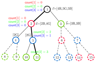
Figure 10: A demonstration of how Algorithm 3 finds the sub-indices of all nodes along the root-to-leaf-11 path in their corresponding color classes. The algorithm performs the color-splitting algorithm (Algorithm 2) only on the nodes along the path and their siblings. Other nodes (dashed) are ignored. When the current node $k$ receives color $i$, it has sub-index $j_{k}=\texttt{count}[i]+1$ in the color class $C_{i}$. Thus, node 2 is the first node among the reds, node 5 is the second among the blues, and node 11 is the forth among the green.

Example 4.

Consider the tree of height $h=3$ in Fig. 10, in which the path 1-2-5-11 is considered. Let colors $i=1,2,3$ denote Red, Green, and Blue, respectively. As the algorithm colors node 2 red and node 3 green, and gives three reds and three blues to the right branch, at node 2 (treated as the current node), the count array is updated as follows:

• $\texttt{count}[1][1]=0$ (unchanged). As node 2 receives color $1$ (Red), it has sub-index $j_{2}=\texttt{count}[1]+1=1$ in $C_{1}$.

• $\texttt{count}[2][1]=0$ (unchanged).

• $\texttt{count}[3][1]=0$ (unchanged).

The algorithm continues in a similar manner. Once it reaches the leaf 11, it has found all the sub-indices of nodes 2, 5, 11 in the corresponding color classes: $j_{2}=1$, $j_{5}=2$, and $j_{11}~{}=~{}4$. This is correct given that the color classes are arranged according to the left-right order, with ${\color[rgb]{1,0,0}C_{1}=\{2,6,14,15\}}$, ${\color[rgb]{0,1,0}C_{2}=\{8,9,10,11,3\}}$, and ${\color[rgb]{0,0,1}C_{3}=\{4,5,12,13,7\}}$.

1:  Input: Tree height $h$, a leaf index $j\in[2^{h},\ldots,2^{h+1}-1]$, $h$ node indices $k_{1},\ldots,k_{h}$, and an $h$-feasible color sequence $\vec{c}=(c_{1},\ldots,c_{h})$;  

2:  Initialize an array $\texttt{idx}[h]$ to hold the output sub-indices of nodes $k_{1},\ldots,k_{h}$ in their corresponding color classes;

3:  Initialize an array $\texttt{count}[h]$ as follows:$\texttt{count}[i]:=0$ for $i=1,2,\ldots,h$;

4:  $R:=1$;

5:  for $\ell=1$ to $h-1$ do

6:     Let $\texttt{sb}_{\ell}$ be the sibling node of $k_{\ell}$; // $\texttt{sb}_{\ell}:=k_{\ell}-1$ or $k_{\ell}+1$

7:     Assign Color $i_{\ell}$ to $k_{\ell}$ and Color $i^{\prime}_{\ell}$ to $\texttt{sb}_{\ell}$; // Following lines 3-7 in ColorSplittingRecursive, note that it is possible that $i_{\ell}=i^{\prime}_{\ell}$

8:     $\texttt{is\_left}:=\text{True}$ if $k_{\ell}$ is the left child of $R$, and False otherwise; // if $k_{\ell}=2R$ then it is the left child of $R$

9:     Let $\vec{a}$ and $\vec{b}$ be the output color sequences of FeasibleSplit$(h-\ell+1,\vec{c})$; // time complexity $\mathcal{O}(h)$

10:     $\vec{c}:=\vec{a}$ if $\texttt{is\_left}=\text{True}$, and $\vec{c}:=\vec{b}$ otherwise;

11:     UpdateCount$(\texttt{count},i_{\ell},i^{\prime}_{\ell},\texttt{is\_left},\vec{a},\vec{b})$; // $\mathcal{O}(h^{2})$

12:     $\texttt{idx}[\ell]:=\texttt{count}[i_{\ell}]+1$; // the sub-index of $k_{\ell}$ in $C_{i}$

13:     $R:=k_{\ell}$; // move down to the child node $k_{\ell}$

14:  end for

15:  Let $i_{h}$ be the only color left in $\vec{c}$; // $\vec{c}=[2]$, e.g. two greens

16:  Update $\texttt{count}[i_{h}]:=\texttt{count}[i_{h}]+1$ if $k_{h}$ is the right child of $k_{h-1}$; // if it is the left child, do nothing

17:  $\texttt{idx}[h]:=\texttt{count}[i_{h}]+1$; // the sub-index of $k_{h}$ in $C_{i_{h}}$

18:  return  idx;

Algorithm 3 Find Sub-Indices

1:  for $i=1$ to $h$ do

2:     if is_left = False AND $\vec{b}[i]\neq 0$ then

3:        Find the number $l_{i}$ of Color $i$ given to $\vec{a}$; // $\mathcal{O}(h)$

4:        $\texttt{count}[i]:=\texttt{count}[i]+l_{i}$; // Gaining $l_{i}$ nodes of Color $i$ on the left side of $k_{\ell}$ (excluding the sibling)

5:        if $i=i^{\prime}_{\ell}$ then

6:           $\texttt{count}[i]:=\texttt{count}[i]+1$; // Gaining one node of Color $i$ (due to the sibling receiving colore $i$) on the left side of $k_{\ell}$

7:        end if

8:     end if

9:  end for

Procedure UpdateCount$(\texttt{count},i_{\ell},i^{\prime}_{\ell},\texttt{is\_left},\vec{a},\vec{b}))$

V Experiments and Evaluations

V-A Experimental setup

We ran our experiments on Ubuntu 22.04.1 environment (Intel Core i5-1035G1 CPU @1.00GHz×8, 15GiB System memory) for the client side and until 30 PIR servers on Amazon t2.large instances (Intel(R) Xeon(R) CPU E5-2686 v4 @ 2.30GHz, 2 vCPUs, 8GiB System Memory). We utilize the HTTP/2 protocol in conjunction with gRPC version 35.0.0 [55], which is developed by Google, for connecting numerous clients and servers over the network. The code used for our experiments is available on GitHub [56].

Bitcoin datasets. We utilized our Java code [56] to gather 200 Bitcoin Blocks [57] from the Block 813562, containing 2390 transactions, mined on 2023-10-24 at 09:52:26 GMT +11, to Block 813363, which included 2769 transactions and was mined on 2023-10-23 at 04:13:24 GMT +11. On average, within the dataset we collected, there were 1839 transactions in each Block. The number of transactions in each Bitcoin Block typically ranges from 1000 to 4500 [57], and the number of active addresses per day is more than 900K [58]. To interface with the Blockchain Data API [57] for collecting real-time Bitcoin Blocks in JSON format, we used HttpURLConnection and Google GSON 2.10.1 [59].

Baselines. Our Coloring method can be applied on top of any PIR schemes, allowing us to optimize with other Batched PIR solutions [18, 39] following baselines:

- One Client parallel privately retrieves a Merkle proof:

+ Angle et al.’s batchPIR (SealPIR+PBC) [18] employs SealPIR as the foundational PIR. Note that (SealPIR+PBC) uses $m=1.5h$ databases of size $2N/h$ each.

+ $h$-Repetition (see Remark 1), which is a trivial solution repeated $h$ times SealPIR on top of the whole tree.

+ Proof-as-Element is applied SealPIR once on a database where each element is a Merkle proof ($h$ hashes).

+ Layer-based, which is a trivial coloring solution repeated $h$ times SealPIR on each layer of the tree.

We did not include Vectorized BatchPIR (VBPIR) [42] in the comparisons because we hadn’t found a way to implement a parallel version of their scheme at the time of submission. However, as noted in [42], in their experiment, VBPIR had communication cost $20$-$96\times$ smaller than (SealPIR+PBC), but with a slightly higher computation cost ($1.1\times$ to $1.6\times$ higher).

- Multiple Clients parallel privately retrieve multiple Merkle proofs:

Albab et al.’s BatchPIR (DP-PIR) [39] has shown the capability to efficiently manage large query batches, especially when the ratio $\frac{q}{N}>10$. To illustrate this with a real-world example related to Bitcoin, it is worth noting that a Bitcoin Block contains an average of approximately $6$K addresses [58]. Suppose all $6$K clients want to retrieve their Merkle proofs privately. In this case, they must batch $6,000\times h$ queries. For instance, with a tree height of $h=10$, the ratio $\frac{q}{N}=\frac{60,000}{2,046}>10$, making DP-PIR a suitable choice. When we consider the tree coloring method, where each client privately retrieves a node from each color database, the ratio $\frac{q}{N}=\frac{6,000}{205}$ remains greater than 10. However, our DP-PIR+Coloring approach performs parallel processing on each smaller database and fewer batch queries. As a result, our method significantly reduces the computation time in both online and offline phases (see Table IV).

Schemes	Computation (parallel)		Communication
(BatchPIR)	Online	Offline	Online	Offline
DP-PIR [39]	$\mathcal{O}(N+hc)$	$\mathcal{O}(N+hc)$	$\mathcal{O}(hc)$	$\mathcal{O}(hc)$
DP-PIR+Coloring	$\mathcal{O}(\frac{N}{h}+c)$	$\mathcal{O}(\frac{N}{h}+c)$	$\mathcal{O}(hc)$	$\mathcal{O}(hc)$

TABLE IV: Communication and computation complexity of our scheme and DP-PIR scheme. Here, $N$ and $h$ denote the number of tree nodes and the tree height, respectively, and $c$ clients wants to receive $c$ Merkle proofs privately.

Color-Splitting Algorithm setup. Our Java code was compiled using Java OpenJDK version 11.0.19 on Amazon c6i.8xlarge instance (Intel(R) Xeon(R) Platinum 8375C CPU @ 2.90GHz, 32 vCPUs, 64GiB System Memory). We ran the code 100 times for each tree with the number of leaves $n$ ranging from $2^{10}$ to $2^{20}$ and calculated the average. The running times are presented in Fig. 11, which confirm the theoretical complexity (almost linear) of our algorithm. Note that the algorithm only ran on a single vCPU of the virtual machine. Our current code can handle trees of heights upto $35$, for which the algorithm took 2.5 hours to complete. For a perfect binary tree of height $h=30$, it took less than 5 minutes to produce a balanced ancestral coloring.

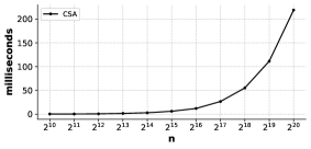
Figure 11: The average running times of the Color-Splitting Algorithm (CSA) when generating balanced ancestral colorings for the perfect binary trees with $n=2^{10},2^{11},\ldots,2^{20}$ leaves. For each $n$, the algorithm was run a hundred times and the average running time was recorded.

One Client parallel privately retrieves a Merkle proof setup. As described, we used until 30 Amazon t2.large instances with 2 vCPUs. Our implementation is single core per instance per server for ease of comparison with prior works. We used until 30 instances because with $h=20$, SealPIR+PBC generated 30 databases, each of server processed a PIR database of size approximately $200$K elements while our scheme used only 20 servers, each of which handled a PIR database of size roughly $100$K elements (see Table V). We compiled our C++ code with Cmake version 3.22.1 and Microsoft SEAL version 4.0.0 [60]. Our work focuses on the perfect Merkle tree, so we collected the latest Bitcoin transactions to make the Merkle tree perfect. As Bitcoin, our Java code generated the Block’s Merkle tree using the SHA-256 hash function. Hence, each tree node had a size of 256 bits (hash digit size).

Schemes (BatchPIR)	Number of servers	Largest database size	Total storage
Proof-as-Element	1	$n\times h$	$n\times h$
$h$-Repetition	$h$	$N$	$h\times N$
Layer-based	$h$	$n$	$N$
SealPIR+PBC [18]	$\lceil 1.5\times h\rceil$	$\lceil\frac{2\times N}{h}\rceil$	$3N$
SealPIR+Coloring	$h$	$\lceil\frac{N}{h}\rceil$	$N$

TABLE V: Experimenting with varying server quantities. Our experiments involved running servers in parallel, where the server processing the largest database took the most time. Here, $N$, $h$, and $n$ denote the number of tree nodes, the tree height, and the number of leaves, respectively.

Multiple Clients parallel privately retrieve multiple Merkle proofs setup. For simplicity, we ran our experiments on a local Ubuntu 22.04.1 environment (Intel Core i5-1035G1 CPU @1.00GHz×8, 15GiB System memory). We employed two servers and one client, which acted as multiple clients, following the same settings described in DP-PIR [61].

V-B Evaluations

We present in Fig. 12 the (parallel) servers times required by different retrieval schemes. Our solution always performed better than others and took less than 0.2 seconds when $n=2^{20}$. In Table V, our approach employs batched SealPIR based on our tree coloring methods, resulting in the smallest PIR database and minimal storage overhead. As a result, our solution demonstrates the fastest performance, especially for larger $h$ (larger saving).

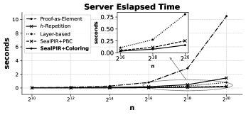
Figure 12: A comparison of the server computation costs in parallel of five schemes from $n=2^{10}$ to $n=2^{20}$. Our coloring-based scheme outperforms others. Size of each node is 32 bytes (hash digest size).

Observe that both the total client computation costs and communication costs increase with the batch size (see Figures 13 and 14). As mentioned earlier, SealPIR+PBC [18] requires $\lceil 1.5h\rceil$ databases while most others require $h$ databases. As a result, the client computation and total communication costs associated with SealPIR were consistently the highest, and others were lower and almost equal. On the other hand, the Proof-as-Element approach only requires a single database, making it the method with the lowest and nearly constant client computation and total communication costs. However, this scheme required the longest server computation time (see Fig. 12).

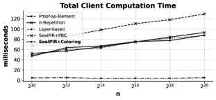
Figure 13: A comparison of the total client computation costs of five schemes from $n=2^{10}$ to $n=2^{20}$. Size of each node is 32 bytes (hash digest size).

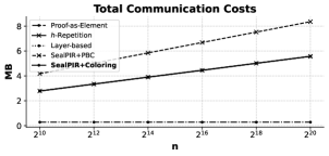
Figure 14: A comparison of the total communication costs (queries + responses) of five schemes from $n=2^{10}$ to $n=2^{20}$. Size of each node is 32 bytes.

For handling large batches of queries, DP-PIR is very efficient. In Fig. 15, the DP-PIR scheme moved most of the computation costs in the Offline phase, and the Online cost is faster than the Offline phase $500\times$. However, when combining DP-PIR with our coloring scheme, our solution improved $h\times$ both Online and Offline time.

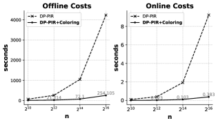
Figure 15: The computation time for DP-PIR and DP-PIR+Coloring, both online and offline, was evaluated from $n=2^{10}$ to $n=2^{16}$ while retrieving 6000 Merkle proofs privately.

When a Merkle tree of height $h$ is partitioned with a balanced ancestral coloring, it enables us to significantly accelerate the private retrieval of Merkle proofs in the arbitrary parallel PIR model in the server side. We have outperformed other batchPIR solutions through our implementation, providing strong evidence supporting our theoretical argument.

VI Conclusions

We consider in this work the problem of private retrieval of Merkle proofs in a Merkle tree, which has direct applications in various systems that provide data verifiability feature such as Amazon DynamoDB, Google’s Certificate Transparency, and blockchains. By exploiting a unique feature of Merkle proofs, we propose a new parallel retrieval scheme based on the novel concept of ancestral coloring of trees, allowing an optimal storage overhead and a reduced computational complexity compared to existing schemes. In particular, our tree coloring/partitioning solution can be used to replace the (probabilistic) batch code component in several batch-code-based retrieval schemes developed in the literature to improve their performance.

For the parallel private retrieval of Merkle proofs to work, one needs to use an ancestral coloring to partition the tree into equal parts such that ancestor-descendant nodes never belong to the same part. We establish a necessary and sufficient condition for an ancestral coloring of arbitrary color class sizes to exist (for perfect binary trees of any height), and develop an efficient divide-and-conquer algorithm to find such a coloring (if any). We are currently working on extending the coloring algorithm to deal with $q$-ary trees, which are an essential component in various blockchains. Tackling dynamically growing Merkle trees is another open practical problem that might require some significant extension of our current understanding of tree colorings.

Appendix A Private Index Retrieval

The private index retrieval (PIXR) problem provides a way for the client who possesses a item in a database to privately retrieve the index of the item. A solution to this problem can be used in a PIR problem to enable the client to find out the required index of the item to retrieve, or to be used as a solution to the indexing problem described in Section III-B regarding ancestral coloring. The communication and computation overheads are the main performance metrics. We describe this problem and and propose a solution with low communication overhead below.

A server stores a list of $n$ distinct $k$-bit vectors $v_{1},\ldots,v_{n}$. A client possesses a vector $v$, among the $n$ vectors. The client wishes to know the index $i\in\{1,2,\ldots,n\}$ so that $v=v_{i}$. Suppose that $n$ and $k$ are known a priori. What is the most efficient method (in terms of computation and communication costs) for the client to extract this index without revealing $v$ to the server? Because SHA256 is the most widely used hash function in the context of Merkle trees, we usually have $k=256$. Moreover, we experiment with $n=2^{h}$ where $10\leq h\leq 20$. Note that in our experiments, instead of using blockchain transactions, we use their 256-bit hashes as $v_{i}$, which are at least $8$ times smaller than the transactions themselves.

A trivial approach to determining the index $i$ is for the client to download the entire list of $n$ vectors and compare them one by one against $v$ to find $i$ satisfying $v=v_{i}$. This approach requires no computation at the server side but a computation complexity of $\mathcal{O}(n)$ at the client side and a communication cost of $\mathcal{O}(kn)$ bits.

To reduce the communication cost, we observe that when $k$ is much greater than $\log_{2}(n)$, we usually do not need all $k$ bits to distinguish the $n$ vectors. This observation is relevant as we often deal with $k=256$ and $n=2^{h}$ where $h\ll 256$. If only communication cost is our concern, then this is precisely the Distinct Vectors Problem, which was first discussed in [62]: the goal is to find a minimum set of bits among $k$ bits that can still distinguish all $n$ vectors. It was shown in [62] that the problem is NP-hard. However, in the context of our work, where the vectors are 256-bit hashes and can be effectively treated as randomly distributed vectors, $2\log_{2}n$ bits are usually enough to distinguish $n$ vectors (in contrast to the worst case where all $k$ bits may be required to distinguish the vectors). Indeed, the probability that $n$ random $(2\log_{2}n)$-bit vectors are pairwise distinct is $p(n)=\prod_{i=1}^{n}\frac{n^{2}-i}{n^{2}}$, which is sufficiently large. The minimum number of bits often lies between $\log_{2}n$ and $2\log_{2}n$, so $2\log_{2}n$ provides a sufficiently good approximation. This observation has also been confirmed through extensive experiments on several sets of hashes of real Bitcoin transactions. Note that the proposed method requires some extra computation at the server side (performed once only) and the same computation cost (if not faster) at the client side as in the trivial method. Moreover, the communication cost is reduced by a factor of $k/2\log_{2}n$, which ranges from 4x to 12x for $n=2^{h}$, $10\leq h\leq 30$ when $k=256$.

Number of transactions	Vector length	Average run time	Average number of steps
$2^{10}$	20 bits	7 ms	1.6
$2^{12}$	24 bits	16 ms	2.3
$2^{14}$	28 bits	55 ms	1.7
$2^{16}$	32 bits	226 ms	1.3
$2^{18}$	36 bits	705 ms	1.4
$2^{19}$	38 bits	1700 ms	1.7
$2^{20}$	40 bits	3668 ms	1.5

TABLE VI: The running time of the algorithm at the server side that finds a set of $2\log_{2}n$ bits that can distinguish $n$ 256-bit hashes. These hashes are from real transactions collected from blockchain.com API. The measured running times were averaged over 10 datasets of each size and confirmed the theory that only $2\log_{2}n$ bits are usually required to distinguish $n$ $256$-bit hashes.

We ran a simple algorithm that extracts $2\log_{2}n$ bits that distinguish all $n$ hashes of transactions downloaded from blockchain.com API [63]. The algorithm checks whether the set of the first $2\log_{2}n$ bits can be used to distinguish all the hashes (using a hash table). If Yes, then it returns these bit positions (providing the position of the first bit is enough as they are consecutive), if No, then it jumps to the next set of $2\log_{2}n$ bits and repeats the test, and so on. For each size $n$, we ran our experiment on $10$ different datasets and took the average measurement.

As shown in Table VI, the algorithm only needs to check 1 to 2 sets of $2\log_{2}n$ bits before obtaining relevant bit sets. Moreover, the running times are relatively low. Note that this is a one-off computation for each Merkle tree on the server.

Appendix B Proof of Lemma 3

Proof.

Note that because the Color-Splitting Algorithm starts off with the desirable color sequence $\vec{c}$, if it terminates successfully then the output coloring, according to Lemma 2, will be the desirable ancestral $\vec{c}$-coloring. Therefore, our remaining task is to show that the Color-Splitting Algorithm always terminates successfully. Both ColorSplittingRecursive$(R,h,\vec{c})$ and FeasibleSplit$(h,\vec{c})$ work if $c_{1}\geq 2$ when $h\geq 1$, i.e., when the current root node still has children below. This condition holds trivially in the beginning because the original color sequence is feasible. To guarantee that $c_{1}\geq 2$ in all subsequent algorithm calls, we need to prove that starting from an $h$-feasible color sequence $\vec{c}$ with $h\geq 2$, FeasibleSplit$(h,\vec{c})$ always produces two $(h-1)$-feasible color sequences $\vec{a}$ and $\vec{b}$ for the two subtrees. This is the most technical and lengthy part of the proof of correctness of CSA and will be settled separately in Lemma 5 and Lemma 6.

In the remainder of the proof of this lemma, we analyze the time complexity of CSA. Let $C(n)$, $n=2^{h}$, be the number of basic operations (e.g., assignments) required by the recursive procedure ColorSplittingRecursive$(R,h,\vec{c})$. Then from its description, the following recurrence relation holds

$$C(n)=\begin{cases}2C(n/2)+\alpha h\log(h),&\text{ if }n\geq 4,\\ \beta,&\text{ if }n=2,\end{cases}$$

where $\alpha$ and $\beta$ are positive integer constants and $\alpha h\log h$ is the running time of FeasibleSplit$(h,\vec{c})$ (dominated by the time required for sorting $\vec{a}$ and $\vec{b}$), noting that $h=\log_{2}n$. We can apply the backward substitution method (or an induction proof) to determine $C(n)$ as follows.

$$\begin{split}C(n)&=2C(n/2)+\alpha h\log h\\ &=2\big{(}2C(n/2^{2})+\alpha(h-1)\log(h-1)\big{)}+\alpha h\log h\\ &=2^{2}C(n/2^{2})+\alpha\big{(}2(h-1)\log(h-1)+h\log h\big{)}\\ &=\cdots\\ &=2^{k}C(n/2^{k})+\alpha\sum_{i=0}^{k-1}2^{i}(h-i)\log(h-i),\end{split}$$

for every $1\leq k\leq h-1$. Substituting $k=h-1$ in the above equality and noting that $C(2)=\beta$, we obtain

$$C(n)=\beta 2^{h-1}+\alpha\sum_{i=0}^{h-1}2^{i}(h-i)\log(h-i)\\ \leq\beta 2^{h-1}+\alpha\bigg{(}h\sum_{i=0}^{h-1}2^{i}-\sum_{i=0}^{h-1}i2^{i}\bigg{)}\log h\\ =\beta 2^{h-1}+\alpha\big{(}h(2^{h}-1)-((h-2)2^{h}+2)\big{)}\log h\\ =\beta 2^{h-1}+\alpha(2^{h+1}-h+2)\log h\in\mathcal{O}(2^{h+1}\log h)\\ =\mathcal{O}(n\log\log n).$$

Therefore, as claimed, the Color-Splitting Algorithm has a running time $O\big{(}2^{h+1}\log h\big{)}$. ∎

Appendix C Proof of Lemma 4

Proof.

We consider two cases based on the parity of $c$.

Case 1: $c$ is even. In this case, from (P3) we have $a_{m+1}=\cdots=a_{\ell}=a$, where $a\triangleq c/2$. As $p>m$, we have $S_{p}=S_{m}+\sum_{i=m+1}^{p}a_{i}$. If $S_{m}\geq\sum_{i=1}^{p}2^{i}$ then the conclusion trivial holds. Otherwise, let $S_{m}=\sum_{i=1}^{p}2^{i}-\delta$, for some $\delta>0$. Then (P1) implies that

$$0<\delta=\sum_{i=1}^{p}2^{i}-S_{m}\leq\sum_{i=1}^{p}2^{i}-\sum_{i=1}^{m}2^{i}=\sum_{i=m+1}^{p}2^{i}.$$ (1)

Moreover, from (P2) we have

$$S_{\ell}=S_{m}+(\ell-m)a=\bigg{(}\sum_{i=1}^{p}2^{i}-\delta\bigg{)}+(\ell-m)a\geq\sum_{i=1}^{\ell}2^{i},$$

which implies that

$$a\geq\frac{1}{\ell-m}\bigg{(}\sum_{i=p+1}^{\ell}2^{i}+\delta\bigg{)}.$$

Therefore,

$$S_{p}=S_{m}+(p-m)a=\bigg{(}\sum_{i=1}^{p}2^{i}-\delta\bigg{)}+(p-m)a\\ \geq\bigg{(}\sum_{i=1}^{p}2^{i}-\delta\bigg{)}+\frac{p-m}{\ell-m}\bigg{(}\sum_{i=p+1}^{\ell}2^{i}+\delta\bigg{)}.$$

Hence, in order to show that $S_{p}\geq\sum_{i=1}^{p}2^{i}$, it suffices to demonstrate that

$$(p-m)\sum_{i=p+1}^{\ell}2^{i}\geq(\ell-p)\delta.$$

Making use of (1), we need to show that the following inequality holds

$$(p-m)\sum_{i=p+1}^{\ell}2^{i}\geq(\ell-p)\sum_{i=m+1}^{p}2^{i},$$

which is equivalent to

$$\frac{\sum_{i=p+1}^{\ell}2^{i}}{\sum_{i=m+1}^{p}2^{i}}\geq\frac{\ell-p}{p-m}\Longleftrightarrow\frac{2^{p-m}(2^{\ell-p}-1)}{2^{p-m}-1}\geq\frac{\ell-p}{p-m}.$$

The last inequality holds because $\frac{2^{p-m}}{2^{p-m}-1}>1\geq\frac{1}{p-m}$ and $2^{\ell-p}-1\geq\ell-p$ for all $0\leq m<p<\ell$. Here we use the fact that $2^{x}-1-x\geq 0$ for all $x\geq 1$. This establishes Case 1.

Case 2: $c$ is odd. In this case, from (P3) we have $a_{m+1}=\cdots=a_{m+k}=a$ and $a_{m+k+1}=\cdots=a_{\ell}=a+1$, where $a\triangleq\lfloor c/2\rfloor$. We claim that if the inequality

$$S_{m+k}\geq\sum_{i=1}^{m+k}2^{i}$$ (2)

holds then we can reduce Case 2 to Case 1. Indeed, suppose that (2) holds. Then by replacing $\ell$ by $m+k$ and applying Case 1, we deduce that $S_{p}\geq\sum_{i=1}^{p}2^{i}$ for every $p$ satisfying $m<p<m+k$. Similarly, by replacing $m$ by $m+k$ and applying Case 1, the inequality $S_{p}\geq\sum_{i=1}^{p}2^{i}$ holds for every $p$ satisfying $m+k<p<\ell$. Thus, in the remainder of the proof, we aim to show that (2) is correct.

To simplify the notation, set $p\triangleq m+k$. If $p=m$ or $p=\ell$ then (P1) and (P2) imply (2) trivially. Thus, we assume that $m<p<\ell$. Since $S_{p}=S_{m}+\sum_{i=m+1}^{p}a_{i}$, if $S_{m}\geq\sum_{i=1}^{p}2^{i}$ then the conclusion trivial holds. Therefore, let $S_{m}=\sum_{i=1}^{p}2^{i}-\delta$, for some $\delta>0$. Similar to Case 1, (P1) implies that

$$0<\delta=\sum_{i=1}^{p}2^{i}-S_{m}\leq\sum_{i=1}^{p}2^{i}-\sum_{i=1}^{m}2^{i}=\sum_{i=m+1}^{p}2^{i}.$$ (3)

Moreover, from (P2) we have

$$S_{\ell}=S_{m}+(\ell-m)a+(\ell-p)\\ =\bigg{(}\sum_{i=1}^{p}2^{i}-\delta\bigg{)}+(\ell-m)a+(\ell-p)\geq\sum_{i=1}^{\ell}2^{i},$$

which implies that

$$a\geq\frac{1}{\ell-m}\bigg{(}\sum_{i=p+1}^{\ell}2^{i}+\delta-(\ell-p)\bigg{)}.$$

Therefore,

$$S_{p}=S_{m}+(p-m)a=\bigg{(}\sum_{i=1}^{p}2^{i}-\delta\bigg{)}+(p-m)a\\ \geq\bigg{(}\sum_{i=1}^{p}2^{i}-\delta\bigg{)}+\frac{p-m}{\ell-m}\bigg{(}\sum_{i=p+1}^{\ell}2^{i}+\delta-(\ell-p)\bigg{)}.$$

Hence, in order to show that $S_{p}\geq\sum_{i=1}^{p}2^{i}$, it suffices to demonstrate that

$$(p-m)\bigg{(}\sum_{i=p+1}^{\ell}2^{i}-(\ell-p)\bigg{)}\geq(\ell-p)\delta.$$

Making use of (3), we need to show that the following inequality holds

$$(p-m)\bigg{(}\sum_{i=p+1}^{\ell}2^{i}-(\ell-p)\bigg{)}\geq(\ell-p)\sum_{i=m+1}^{p}2^{i},$$

which is equivalent to

$$\begin{split}&\frac{\sum_{i=p+1}^{\ell}2^{i}-(\ell-p)}{\sum_{i=m+1}^{p}2^{i}}\geq\frac{\ell-p}{p-m}\\ &\Longleftrightarrow\frac{2^{p-m}(2^{\ell-p}-1)-(\ell-p)/2^{m+1}}{2^{p-m}-1}\geq\frac{\ell-p}{p-m}.\end{split}$$ (4)

If $\ell-p=1$ then the last inequality of (4) becomes

$$\frac{2^{p-m}-1/2^{m+1}}{2^{p-m}-1}\geq\frac{1}{p-m},$$

which is correct because $1/2^{m+1}<1$ and $p-m\geq 1$. If $\ell-p\geq 2$ then the last inequality of (4) can be rewritten as

$$\frac{2^{p-m}}{2^{p-m}-1}\bigg{(}2^{\ell-p}-1-\frac{\ell-p}{2^{p+1}}\bigg{)}\geq\frac{\ell-p}{p-m},$$

which is correct because $\frac{2^{p-m}}{2^{p-m}-1}>1\geq\frac{1}{p-m}$ for $p>m$ and

$$2^{\ell-p}-1-\frac{\ell-p}{2^{p+1}}\geq 2^{\ell-p}-1-\frac{\ell-p}{4}\geq\ell-p,$$

noting that $p\geq 1$ and that $2^{x}-1-\frac{5}{4}x>0$ for every $x\geq 2$. This establishes Case 2. ∎

Appendix D Proof of Lemma 5

Proof.

To make the proof more readable, let $\vec{a}^{\prime}=[a^{\prime}_{2},\ldots,a^{\prime}_{h}]$ and $\vec{b}^{\prime}=[b^{\prime}_{2},\ldots,b^{\prime}_{h}]$ be obtained from $\vec{a}$ and $\vec{b}$ after their elements are sorted in non-decreasing order. According to Definition 6, the goal is to show that (C1) and (C2) hold for $\vec{a}^{\prime}$ and $\vec{b}^{\prime}$, while replacing $h$ by $h-1$. Because the sums $S_{i}(a)\triangleq\sum_{j=2}^{i}a_{i}$ and $S_{i}(b)\triangleq\sum_{j=2}^{i}b_{i}$ always differ from each other by at most one for every $2\leq i\leq h$, it is clear that at the end when $i=h$, they should be the same and equal to half of $S_{h}(c)\triangleq\sum_{j=2}^{h}c_{j}=\sum_{j=2}^{h}2^{j}=2\big{(}\sum_{j=1}^{h-1}2^{j}\big{)}$. Therefore, (C2) holds for $\vec{a}$ and $\vec{b}$ and hence, for $\vec{a}^{\prime}$ and $\vec{b}^{\prime}$ as well. It remains to show that (C1) holds for these two color sequences, that is, to prove that $\sum_{i=2}^{\ell}a^{\prime}_{i}\geq\sum_{i=1}^{\ell-1}2^{i}$ and $\sum_{i=2}^{\ell}b^{\prime}_{i}\geq\sum_{i=1}^{\ell-1}2^{i}$ for every $2\leq\ell\leq h$ (note that $\vec{a}^{\prime}$ and $\vec{b}^{\prime}$ both start from index 2).

Since $a_{i}$ and $b_{i}$ are assigned either $\lfloor c_{i}/2\rfloor$ or $\lceil c_{i}/2\rceil$ in somewhat an alternating manner, which keeps the sums $S_{i}(a)\triangleq\sum_{j=2}^{i}a_{i}$ and $S_{i}(b)\triangleq\sum_{j=2}^{i}b_{i}$ differ from each other by at most one, it is obvious that each sum will be approximately half of $\sum_{j=2}^{i}c_{j}$ (rounded up or down), which is greater than or equal to $\sum_{j=2}^{i}2^{j}=2\big{(}\sum_{j=1}^{i-1}2^{j}\big{)}$. Therefore, (C1) holds for $\vec{a}$ and $\vec{b}$. However, the trouble is that this may no longer be true after sorting, in which smaller values are shifted to the front. We show below that (C1) still holds for $\vec{a}^{\prime}$ and $\vec{b}^{\prime}$ using Lemma 4.

As $\vec{c}$ is a sorted sequence, we can partition $c_{2},c_{3},\ldots,c_{h}$ into $k$ different runs where within each run all $c_{i}$’s are equal,

$$c_{2}=\cdots=c_{i_{1}}<c_{i_{1}+1}=\cdots=\\ c_{i_{2}}<\cdots<c_{i_{k-1}+1}=\cdots=c_{i_{k}}\equiv c_{h}.$$ (5)

For $r=1,2,\ldots,k$, let $R_{r}\triangleq[i_{r-1}+1,i_{r}]$, where $i_{0}\triangleq 1$. Then (5) means that for each $r\in[k]$, $c_{i}$’s are the same for all $i\in R_{r}$ and moreover, $c_{i}<c_{i^{\prime}}$ if $i\in R_{r}$, $i^{\prime}\in R_{r^{\prime}}$, and $r<r^{\prime}$. In order to show that (C1) holds for $\vec{a}^{\prime}$ and $\vec{b}^{\prime}$, our strategy is to first prove that (C1) holds for $\vec{a}^{\prime}$ and $\vec{b}^{\prime}$ at the end-points $\ell=i_{r}$ of the runs $R_{r}$, $r\in[k]$, and then employ Lemma 4 to conclude that (C1) also holds for these color sequences at all the middle-points of the runs.

Since $\lfloor c_{i}/2\rfloor\leq a_{i}\leq\lceil c_{i}/2\rceil$ for every $2\leq i\leq h$, it is clear that $a_{i}\leq a_{i^{\prime}}$ if $i\in R_{r}$, $i^{\prime}\in R_{r^{\prime}}$, and $r<r^{\prime}$. Therefore, $\vec{a}^{\prime}$ can be obtained from $\vec{a}$ by sorting its elements locally within each run. As a consequence, $\sum_{i\in R_{r}}a^{\prime}_{i}=\sum_{i\in R_{r}}a_{i}$ for every $r\in[k]$, which implies that

$$S_{i_{r}}(a^{\prime})\triangleq\sum_{i=2}^{i_{r}}a^{\prime}_{i}=\sum_{i=2}^{i_{r}}a_{i}\geq\sum_{i=1}^{i_{r}-1}2^{i},$$ (6)

where the last inequality comes from the fact that (C1) holds for $\vec{a}$ and $\vec{b}$ (as shown earlier). The inequality (6) implies that (C1) holds for $\vec{a}^{\prime}$ at the end-points $i_{r}$, $r\in[k]$, of the runs. Applying Lemma 4, we deduce that (C1) also holds for $\vec{a}^{\prime}$ at every middle index $p\in R_{r}$ for all $r\in[k]$. Therefore, (C1) holds for $\vec{a}^{\prime}$, and similarly, for $\vec{b}^{\prime}$. This completes the proof. ∎

Appendix E Proof of Lemma 6

Thanks to the trick of arranging $c_{i}$’s into runs of elements of the same values and Lemma 4, a proof for Lemma 6, although still very lengthy, is manageable. Before proving Lemma 6, we need another auxiliary result.

Lemma 7.

Let $h\geq 4$ and $\vec{c}$, $\vec{a}$, and $\vec{b}$ be defined as in Lemma 6. As $\vec{c}$ is a sorted sequence, we can partition its elements from $c_{4}$ to $c_{h}$ into $k$ different runs where within each run all $c_{i}$’s are equal,

$$c_{4}=\cdots=c_{i_{1}}<c_{i_{1}+1}=\cdots\\ =c_{i_{2}}<\cdots<c_{i_{k-1}+1}=\cdots=c_{i_{k}}\equiv c_{h}.$$

For any $1\leq r\leq k$, let $A_{r}\triangleq\sum_{j=4}^{i_{r}}a_{j}$, $B_{r}\triangleq\sum_{j=4}^{i_{r}}b_{j}$, and $C_{r}\triangleq\sum_{j=4}^{i_{r}}c_{j}$. Then $\min\{A_{r},B_{r}\}\geq\left\lfloor\frac{C_{r}}{2}\right\rfloor-1$.

Proof.

First, we have $|(a_{2}+a_{3})-(b_{2}+b_{3})|=|\lceil\frac{c_{3}+c_{1}-c_{2}}{2}\rceil-\lfloor\frac{c_{3}+c_{1}-c_{2}}{2}\rfloor|\leq 1$. Moreover, the way that $a_{i}$ and $b_{i}$ are defined for $i\geq 4$ in Lemma 6 guarantees that

$$|(a_{2}+a_{3}+A_{r})-(b_{2}+b_{3}+B_{r})|\leq 1,$$

which implies that $|A_{r}-B_{r}|\leq 2$. Furthermore, as $a_{i}+b_{i}=c_{i}$ for all $i\geq 4$, we have

$$A_{r}+B_{r}=\sum_{j=4}^{i_{r}}(a_{j}+b_{j})=\sum_{j=4}^{i_{r}}c_{j}=C_{r}.$$

Thus, $\min\{A_{r},B_{r}\}\geq\left\lfloor\frac{C_{r}}{2}\right\rfloor-1$. ∎

Proof of Lemma 6.

We use a similar approach to that of Lemma 5. However, the proof is more involved because we now must take into account the relative positions of $a_{2}$, $a_{3}$, $b_{2}$, and $b_{3}$ within each sequence after being sorted, and must treat $\vec{a}$ and $\vec{b}$ separately. The case with $h=2$ or $3$ is straightforward to verify. We assume $h\geq 4$ for the rest of the proof.

Let $\vec{a}^{\prime}=[a^{\prime}_{2},\ldots,a^{\prime}_{h}]$ and $\vec{b}^{\prime}=[b^{\prime}_{2},\ldots,b^{\prime}_{h}]$ be obtained from $\vec{a}$ and $\vec{b}$ after sorting. According to Definition 6, the goal is to show that (C1) and (C2) hold for these two sequences while replacing $h$ by $h-1$. The proof that (C2) holds for $\vec{a}^{\prime}$ and $\vec{b}^{\prime}$ is identical to that of Lemma 5, implied by the following facts: first, $\sum_{i=2}^{h}a^{\prime}_{i}=\sum_{i=2}^{h}a_{i}$ and $\sum_{i=2}^{h}b^{\prime}_{i}=\sum_{i=2}^{h}b_{i}$, and second, due to the definitions of $a_{i}$ and $b_{i}$, the two sums $\sum_{i=2}^{h}a_{i}$ and $\sum_{i=2}^{h}b_{i}$ are exactly the same and equal to $\frac{1}{2}\big{(}\sum_{j=1}^{h}c_{i}-2\big{)}=\frac{1}{2}\sum_{i=2}^{h}2^{i}=\sum_{i=1}^{h-1}2^{i}$. It remains to show that (C1) holds for these color sequences.

As $\vec{c}$ is a sorted sequence, we partition its elements from $c_{4}$ to $c_{h}$ into $k$ different runs where within each run all $c_{i}$’s are equal,

$$c_{4}=\cdots=c_{i_{1}}<c_{i_{1}+1}=\cdots=c_{i_{2}}<\cdots\\ <c_{i_{k-1}+1}=\cdots=c_{i_{k}}\equiv c_{h}.$$ (7)

For $r=1,2,\ldots,k$, define the $r$-th run as $R_{r}\triangleq[i_{r-1}+1,i_{r}]$, where $i_{0}\triangleq 3$. Then (7) means that for each $r\in[k]$, $c_{j}$’s are the same for all $j\in R_{r}$ and moreover, $c_{j}<c_{j^{\prime}}$ if $j\in R_{r}$, $j^{\prime}\in R_{r^{\prime}}$, and $r<r^{\prime}$. As $\vec{c}$ is $h$-feasible, it satisfies (C1),

$$c_{1}+c_{2}+c_{3}+\sum_{j=4}^{i_{1}}c_{j}+\cdots+\sum_{j=i_{r-1}+1}^{i_{r}}c_{j}=\sum_{j=1}^{i_{r}}c_{j}\geq\sum_{j=1}^{i_{r}}2^{j}.$$

Equivalently, setting $C_{r}\triangleq\sum_{j=4}^{i_{1}}c_{j}+\cdots+\sum_{j=i_{r-1}+1}^{i_{r}}c_{j}$, we have

$$c_{1}+c_{2}+c_{3}+C_{r}\geq\sum_{j=1}^{i_{r}}2^{j}.$$ (8)

We will make extensive use of this inequality later.

In order to show that (C1) holds for $\vec{a}^{\prime}$ and $\vec{b}^{\prime}$, our strategy is to first prove that (C1) holds for these sequences at the end-points $\ell=i_{r}$ of the runs $R_{r}$, $r\in[k]$, and then employ Lemma 4 to conclude that (C1) also holds for these sequences at all the middle-points of the runs. We also need to demonstrate that (C1) holds for $\vec{a}^{\prime}$ and $\vec{b}^{\prime}$ at the indices of $a_{2}$, $a_{3}$, $b_{2}$, and $b_{3}$ within these sorted sequences. Notice the differences with the proof of Lemma 5: first, we consider the runs from $c_{4}$ instead of $c_{2}$, and second, we must take into account the positions of $a_{2},a_{3},b_{2},b_{3}$ relative to the runs within the sorted sequence $\vec{a}^{\prime}$ and $\vec{b}^{\prime}$.

Since $\lfloor c_{i}/2\rfloor\leq a_{i}\leq\lceil c_{i}/2\rceil$ for every $2\leq i\leq\ell$, it is clear that $a_{i}\leq a_{i^{\prime}}$ if $i\in R_{r}$, $i^{\prime}\in R_{r^{\prime}}$, and $r<r^{\prime}$. Therefore, $\vec{a}^{\prime}$ can be obtained from $\vec{a}$ by sorting its elements $a_{4},\ldots,a_{h}$ locally within each run and then inserting $a_{2}$ and $a_{3}$ into their correct positions (to make $\vec{a}^{\prime}$ non-decreasing). The same conclusion holds for $\vec{b}^{\prime}$.

Note also that $a_{2}$ and $a_{3}$ are inserted between runs (unless they are the first or the last element in $\vec{a}^{\prime}$) and do not belong to any run. The same statement holds for $b_{2}$ and $b_{3}$.

First, we show that $\vec{a}^{\prime}$ satisfies (C1). We divide the proof into two cases depending on whether $a_{2}\leq a_{3}$ or not.

(Case a1) $a_{2}\leq a_{3}$. The sorted sequence $\vec{a}^{\prime}$ has the following format in which within each run $R_{r}$ are the elements $a_{j}$, $j\in R_{r}$, ordered so that those $a_{j}=\left\lfloor\frac{c_{j}}{2}\right\rfloor$ precede those $a_{j}=\left\lceil\frac{c_{j}}{2}\right\rceil$. Note that $c_{j}$’s are equal for all $j\in R_{r}$.

$$\underbracket{\hskip 20.0pt\text{runs}\hskip 20.0pt}\ a_{2}\ \underbracket{\hskip 20.0pt\text{runs}\hskip 20.0pt}\ a_{3}\ \underbracket{\hskip 20.0pt\text{runs}\hskip 20.0pt}$$

Note that it is possible that there are no runs before $a_{2}$, or between $a_{2}$ and $a_{3}$, or after $a_{3}$.

In the first sub-case, the index of interest $\ell=i_{r}$ is smaller than the index of $a_{2}$ in $\vec{a}^{\prime}$. In order to show that (C1) holds for $\vec{a}^{\prime}$ at $\ell=i_{r}$, we prove that

$$A_{r}\triangleq\sum_{j=4}^{i_{r}}a_{j}\geq\sum_{j=1}^{i_{r}-3}2^{j},$$ (9)

noting that in this sub-case the set $\{a_{j}\colon 4\leq j\leq i_{r}\}$ corresponds precisely to the set of the first $i_{r}-3$ elements in $\vec{a}^{\prime}$. We demonstrate below that (9) can be implied from (8). Indeed, since $\vec{c}$ is non-decreasing, from (8) we deduce that

$$4C_{r}\geq c_{1}+c_{2}+c_{3}+C_{r}\geq\sum_{j=1}^{i_{r}}2^{j}.$$

Combining this with Lemma 7, we obtain the desired inequality (9) as follows.

$$A_{r}\geq\left\lfloor\frac{C_{r}}{2}\right\rfloor-1\geq\left\lfloor\frac{1}{8}\sum_{j=1}^{i_{r}}2^{j}\right\rfloor-1\\ =\left\lfloor\sum_{j=1}^{i_{r}-3}2^{j}+\frac{14}{8}\right\rfloor-1=\sum_{j=1}^{i_{r}-3}2^{j}.$$

In the second sub-case, the index of interest $\ell$ is greater than or equal to the index of $a_{2}$ but smaller than that of $a_{3}$ in $\vec{a}^{\prime}$. In other words, either $\ell=i_{r}$ is greater than the index of $a_{2}$ or $\ell$ is precisely the index of $a_{2}$ in $\vec{a}^{\prime}$. If the latter occurs, let $i_{r}$ be the end-point of the run preceding $a_{2}$ in $\vec{a}^{\prime}$. To prove that (C1) holds for $\vec{a}^{\prime}$ at $\ell$, in both cases we aim to show that

$$a_{2}+A_{r}\triangleq a_{2}+\sum_{j=4}^{i_{r}}a_{j}\geq\sum_{j=1}^{i_{r}-2}2^{j},$$ (10)

noting that $\{a_{2}\}\cup\{a_{j}\colon 4\leq j\leq i_{r}\}$ forms the set of the first $i_{r}-2$ elements in $\vec{a}^{\prime}$. We demonstrate below that (10) is implied by (8). First, since $\vec{c}$ is non-decreasing, from (8) we deduce that

$$(c_{1}+c_{2})+2C_{r}\geq(c_{1}+c_{2})+(c_{3}+C_{r})\geq\sum_{j=1}^{i_{r}}2^{j},$$

which implies that

$$\frac{c_{1}+c_{2}}{4}+\frac{C_{r}}{2}\geq\frac{1}{4}\sum_{j=1}^{i_{r}}2^{j}=\sum_{j=1}^{i_{r}-2}2^{j}+\frac{3}{2}.$$ (11)

Next, since $c_{2}\geq c_{1}\geq 3$, we have

$$a_{2}=c_{2}-1>\frac{c_{2}}{2}=\frac{2c_{2}}{4}\geq\frac{c_{1}+c_{2}}{4}.$$

Then, by combining this with Lemma 7 and (11), we obtain the following inequality

$$a_{2}+A_{r}>\frac{c_{1}+c_{2}}{4}+\bigg{(}\left\lfloor\frac{C_{r}}{2}\right\rfloor-1\bigg{)}\geq\frac{c_{1}+c_{2}}{4}+\frac{C_{r}-1}{2}-1\\ =\frac{c_{1}+c_{2}}{4}+\frac{C_{r}}{2}-\frac{3}{2}\geq\sum_{j=1}^{i_{r}-2}2^{j}.$$

Thus, (10) follows.

In the third sub-case, the index of interest $\ell$ is greater than or equal to the index of $a_{3}$. In other words, either $\ell=i_{r}$ is greater than the index of $a_{3}$ or $\ell$ is precisely the index of $a_{3}$ in $\vec{a}^{\prime}$. If the latter occurs, let $i_{r}$ be the end-point of the run preceding $a_{3}$ in $\vec{a}^{\prime}$. To prove that (C1) holds for $\vec{a}^{\prime}$ at $\ell$, in both cases we aim to show that

$$a_{2}+a_{3}+\sum_{j=4}^{i_{r}}a_{j}\geq\sum_{j=1}^{i_{r}-1}2^{j},$$ (12)

noting that in this sub-case $\{a_{2},a_{3}\}\cup\{a_{j}\colon 4\leq j\leq i_{r}\}$ forms the set of the first $i_{r}-1$ elements in $\vec{a}^{\prime}$. This turns out to be the easiest sub-case. With the presence of both $a_{2}$ and $a_{3}$ in the sum on the left-hand side of (12), according to the way $a_{i}$ and $b_{i}$ are selected in Lemma 6, we have

$$\left|\left(a_{2}+a_{3}+\sum_{j=4}^{i_{r}}a_{j}\right)-\left(b_{2}+b_{3}+\sum_{j=4}^{i_{r}}b_{j}\right)\right|\leq 1,$$

and since $a_{2}+a_{3}+b_{2}+b_{3}=c_{1}+c_{2}+c_{3}-2$ and $a_{j}+b_{j}=c_{j}$ for $j\geq 4$, we also have

$$\left(a_{2}+a_{3}+\sum_{j=4}^{i_{r}}a_{j}\right)+\left(b_{2}+b_{3}+\sum_{j=4}^{i_{r}}b_{j}\right)\\ =\sum_{j=1}^{i_{r}}c_{j}-2\geq\sum_{j=2}^{i_{r}}2^{j}=2\sum_{j=1}^{i_{r}-1}2^{j},$$

which, together, imply (12). (Case a2) $a_{2}>a_{3}$. The sorted sequence $\vec{a}^{\prime}$ has the following format.

$$\underbracket{\hskip 20.0pt\text{runs}\hskip 20.0pt}\ a_{3}\ \underbracket{\hskip 20.0pt\text{runs}\hskip 20.0pt}\ a_{2}\ \underbracket{\hskip 20.0pt\text{runs}\hskip 20.0pt}$$

Note that it is possible that there are no runs before $a_{3}$, or between $a_{3}$ and $a_{2}$, or after $a_{2}$.

Again, due to Lemma 4, we only need to demonstrate that (C1) holds for $\vec{a}^{\prime}$ at the end-point $i_{r}$ of each run $R_{r}$, $1\leq r\leq k$, and at $a_{2}$ and $a_{3}$.

In the first sub-case, $\ell=i_{r}$ is smaller than the index of $a_{3}$ in $\vec{a}^{\prime}$. As $a_{2}$ and $a_{3}$ are not involved, the same proof as in the first-subcase of Case a1 applies.

In the second sub-case, the index of interest $\ell$ is greater than or equal to the index of $a_{3}$ but smaller than that of $a_{2}$ in $\vec{a}^{\prime}$. In other words, either $\ell=i_{r}$ is greater than the index of $a_{3}$ and smaller than that of $a_{2}$, or $\ell$ is precisely the index of $a_{3}$ in $\vec{a}^{\prime}$. If the latter occurs, let $i_{r}$ be the end-point of the run preceding $a_{3}$ in $\vec{a}^{\prime}$. To prove that (C1) holds for $\vec{a}^{\prime}$ at $\ell$, we aim to show

$$a_{3}+A_{r}\triangleq a_{3}+\sum_{j=4}^{i_{r}}a_{j}\geq\sum_{j=1}^{i_{r}-2}2^{j},$$ (13)

noting that in this sub-case $\{a_{3}\}\cup\{a_{j}\colon 4\leq j\leq i_{r}\}$ forms the set of the first $i_{r}-2$ elements in $\vec{a}^{\prime}$. We demonstrate below that (13) can be implied from (8) in both cases when $i_{r}=4$ and $i_{r}>4$. First, assume that $i_{r}=4$, i.e, $r=1$ and the run $R_{1}$ consists of only one index $4$. Now, (8) can be written as

$$c_{1}+c_{2}+c_{3}+c_{4}\geq\sum_{j=1}^{4}2^{j}=30,$$

and what we need to prove is

$$a_{3}+\left\lfloor\frac{c_{4}}{2}\right\rfloor\geq\sum_{j=1}^{2}2^{j}=6,$$

noting that the element in $\vec{a}^{\prime}$ corresponding to $c_{4}$ is either $\lfloor c_{4}/2\rfloor$ or $\lceil c_{4}/2\rceil$. Equivalently, plugging in the formula for $a_{3}$, what we aim to show is

$$\left\lceil\frac{c_{3}+c_{1}-c_{2}}{2}\right\rceil+\left\lfloor\frac{c_{4}}{2}\right\rfloor\geq 6.$$ (14)

This inequality is correct because

$$\left\lceil\frac{c_{3}+c_{1}-c_{2}}{2}\right\rceil+\left\lfloor\frac{c_{4}}{2}\right\rfloor\geq\left\lceil\frac{c_{1}}{2}\right\rceil+\left\lfloor\frac{c_{4}}{2}\right\rfloor\geq 6,$$

where the first inequality holds because $c_{3}\geq c_{2}$ and the second inequality holds because $c_{1}\geq 3$ and $c_{4}\geq 8$, given that $c_{4}\geq c_{3}\geq c_{2}\geq c_{1}$ and $c_{1}+c_{2}+c_{3}+c_{4}\geq 30$. To complete this sub-case, we assume that $i_{r}>4$. In this scenario, $C_{r}$ in (8) has at least two terms $c_{j}$’s, which are all greater than or equal to $c_{2}$ and $c_{3}$, and hence, $C_{r}\geq c_{2}+c_{3}$. Therefore, using Lemma 7, we have

$$a_{3}+A_{r}=\left\lceil\frac{c_{3}+c_{1}-c_{2}}{2}\right\rceil+A_{r}\geq\left\lceil\frac{c_{1}}{2}\right\rceil+\left(\left\lfloor\frac{C_{r}}{2}\right\rfloor-1\right)\\ >\frac{c_{1}}{4}+\left(\frac{C_{r}-1}{2}-1\right)=\frac{1}{4}(c_{1}+2C_{r})-\frac{3}{2}\\ \geq\frac{1}{4}(c_{1}+c_{2}+c_{3}+C_{r})-\frac{3}{2}\geq\frac{1}{4}\sum_{j=1}^{i_{r}}2^{j}-\frac{3}{2}=\sum_{j=1}^{i_{r}-2}2^{j}.$$

Thus, (13) follows.

In the third sub-case, assume that the index of interest $\ell$ is greater than or equal to the index of $a_{2}$. As both $a_{2}$ and $a_{3}$ are involved, the proof goes exactly the same way as in the third sub-case of Case 1a. Thus, we have shown that $\vec{a}^{\prime}$ also satisfies (C1) and is $(h-1)$-feasible.

Next, we show that $\vec{b}^{\prime}$ satisfies (C1). The proof is very similar to that for $\vec{a}^{\prime}$. We divide the proof into two cases depending on whether $b_{2}\leq b_{3}$ or not.

(Case b1) $b_{2}\leq b_{3}$. The sorted sequence $\vec{b}^{\prime}$ has the following format in which within each run $R_{r}$ are the elements $b_{j}$, $j\in R_{r}$, ordered so that those $b_{j}=\left\lfloor\frac{c_{j}}{2}\right\rfloor$ precede those $b_{j}=\left\lceil\frac{c_{j}}{2}\right\rceil$. Note that $c_{j}$’s are equal for all $j\in R_{r}$.

$$\underbracket{\hskip 20.0pt\text{runs}\hskip 20.0pt}\ b_{2}\ \underbracket{\hskip 20.0pt\text{runs}\hskip 20.0pt}\ b_{3}\ \underbracket{\hskip 20.0pt\text{runs}\hskip 20.0pt}$$

It is possible that there are no runs before $b_{2}$, or between $b_{2}$ and $b_{3}$, or after $b_{3}$.

The proof for the first and the third sub-cases are exactly the same as for $\vec{a}^{\prime}$. We only need to consider the second sub-case, in which the index $\ell$ is greater than or equal to the index of $b_{2}$ but smaller than that of $b_{3}$ in $\vec{b}^{\prime}$. In other words, either $\ell=i_{r}$ is greater than the index of $b_{2}$ or $\ell$ is precisely the index of $b_{2}$ in $\vec{a}^{\prime}$. If the latter occurs, let $i_{r}$ be the end-point of the run preceding $b_{2}$ in $\vec{b}^{\prime}$. To prove that (C1) holds for $\vec{b}^{\prime}$ at $\ell$, we aim to show that

$$b_{2}+B_{r}\triangleq b_{2}+\sum_{j=4}^{i_{r}}b_{j}\geq\sum_{j=1}^{i_{r}-2}2^{j},$$ (15)

noting that in this sub-case $\{b_{2}\}\cup\{b_{j}\colon 4\leq j\leq i_{r}\}$ forms the set of the first $i_{r}-2$ elements in $\vec{b}^{\prime}$. We demonstrate below that (15) can be implied from (8) in both cases when $i_{r}=4$ and $i_{r}>4$. First, assume that $i_{r}=4$, i.e, $r=1$ and the run $R_{1}$ consists of only one index $4$. Now, (8) can be written as

$$c_{1}+c_{2}+c_{3}+c_{4}\geq\sum_{j=1}^{4}2^{j}=30,$$

and what we need to prove is

$$b_{1}+\left\lfloor\frac{c_{4}}{2}\right\rfloor\geq\sum_{j=1}^{2}2^{j}=6,$$

noting that the element in $\vec{b}^{\prime}$ corresponding to $c_{4}$ is either $\lfloor c_{4}/2\rfloor$ or $\lceil c_{4}/2\rceil$. Equivalently, plugging in the formula for $b_{2}$, what we aim to show is

$$(c_{1}-1)+\left\lfloor\frac{c_{4}}{2}\right\rfloor\geq 6,$$

which is correct because $c_{1}\geq 3$ and $c_{4}\geq 8$, given that $c_{4}\geq c_{3}\geq c_{2}\geq c_{1}$ and $c_{4}+c_{3}+c_{2}+c_{1}~{}\geq~{}30$. To complete this sub-case, we assume that $i_{r}>4$. In this scenario, $C_{r}$ in (8) has at least two terms $c_{j}$’s, which are all greater than or equal to $c_{2}$ and $c_{3}$, and hence, $C_{r}\geq c_{2}+c_{3}$. Therefore, using Lemma 7, we have

$$b_{2}+B_{r}=(c_{1}-1)+B_{r}>\frac{c_{1}}{4}+\left(\left\lfloor\frac{C_{r}}{2}\right\rfloor-1\right)\\ \geq\frac{c_{1}}{4}+\left(\frac{C_{r}-1}{2}-1\right)=\frac{c_{1}}{4}+\left(\frac{C_{r}}{2}-\frac{3}{2}\right)\\ =\frac{1}{4}(c_{1}+2C_{r})-\frac{3}{2}\geq\frac{1}{4}(c_{1}+c_{2}+c_{3}+C_{r})-\frac{3}{2}\\ \geq\frac{1}{4}\sum_{j=1}^{i_{r}}2^{j}-\frac{3}{2}=\sum_{j=1}^{i_{r}-2}2^{j}.$$

Thus, (15) follows. (Case b2) $b_{2}>b_{3}$. The sorted sequence $\vec{b}^{\prime}$ has the following format.

$$\underbracket{\hskip 20.0pt\text{runs}\hskip 20.0pt}\ b_{3}\ \underbracket{\hskip 20.0pt\text{runs}\hskip 20.0pt}\ b_{2}\ \underbracket{\hskip 20.0pt\text{runs}\hskip 20.0pt}$$

Note that it is possible that there are no runs before $b_{3}$, or between $b_{3}$ and $b_{2}$, or after $b_{2}$.

Due to Lemma 4, we only need to demonstrate that (C1) holds for $\vec{b}^{\prime}$ at the end-point $i_{r}$ of each run $R_{r}$, $1\leq r\leq k$, and at $b_{2}$ and $b_{3}$. Similar to Case b1, we only need to investigate the second sub-case when the index of interest $\ell$ is greater than or equal to the index of $b_{3}$ but smaller than that of $b_{2}$ in $\vec{b}^{\prime}$. In other words, either $\ell=i_{r}$ is greater than the index of $b_{3}$ and smaller than that of $b_{2}$, or $\ell$ is precisely the index of $b_{3}$ in $\vec{b}^{\prime}$. If the latter occurs, let $i_{r}$ be the end-point of the run preceding $b_{3}$ in $\vec{b}^{\prime}$. To prove that (C1) holds for $\vec{b}^{\prime}$ at $\ell$, we aim to show that

$$b_{3}+B_{r}\triangleq b_{3}+\sum_{j=4}^{i_{r}}b_{j}\geq\sum_{j=1}^{i_{r}-2}2^{j},$$ (16)

noting that in this sub-case $\{b_{3}\}\cup\{b_{j}\colon 4\leq j\leq i_{r}\}$ forms the set of the first $i_{r}-2$ elements in $\vec{b}^{\prime}$. We demonstrate below that (16) can be implied from (8) in both cases when $i_{r}=4$ and $i_{r}>4$. First, assume that $i_{r}=4$, i.e, $r=1$ and the run $R_{1}$ consists of only one index $4$. Now, (8) can be written as

$$c_{1}+c_{2}+c_{3}+c_{4}\geq\sum_{j=1}^{4}2^{j}=30,$$

and what we need to prove is

$$b_{3}+\left\lfloor\frac{c_{4}}{2}\right\rfloor\geq\sum_{j=1}^{2}2^{j}=6,$$

noting that the element in $\vec{b}^{\prime}$ corresponding to $c_{4}$ is either $\lfloor c_{4}/2\rfloor$ or $\lceil c_{4}/2\rceil$. Equivalently, plugging in the formula for $b_{3}$, what we aim to show is

$$c_{2}-c_{1}+\left\lfloor\frac{c_{3}+c_{1}-c_{2}}{2}\right\rfloor+\left\lfloor\frac{c_{4}}{2}\right\rfloor\geq 6.$$

This inequality is correct because

$$\quad c_{2}-c_{1}+\left\lfloor\frac{c_{3}+c_{1}-c_{2}}{2}\right\rfloor+\left\lfloor\frac{c_{4}}{2}\right\rfloor\\ \geq c_{2}-c_{1}+\frac{c_{3}+c_{1}-c_{2}-1}{2}+\frac{c_{4}-1}{2}\\ \geq\frac{c_{3}+c_{4}}{2}-1>6,$$

where the last inequality holds because $c_{3}+c_{4}\geq 16$, given that $c_{4}\geq c_{3}\geq c_{2}\geq c_{1}$ and $c_{1}+c_{2}+c_{3}+c_{4}\geq 30$. To complete this sub-case, we assume that $i_{r}>4$. In this scenario, $C_{r}$ in (8) has at least two terms $c_{j}$’s, which are all greater than or equal to $c_{1}$ and $c_{2}$, and hence, $C_{r}\geq c_{1}+c_{2}$. Therefore, using Lemma 7 and (8), we have

$$b_{3}+B_{r}=\left(c_{2}-c_{1}+\left\lfloor\frac{c_{3}+c_{1}-c_{2}}{2}\right\rfloor\right)+B_{r}\\ \geq\frac{c_{2}+c_{3}-c_{1}-1}{2}+\left(\left\lfloor\frac{C_{r}}{2}\right\rfloor-1\right)\\ \geq\frac{c_{3}-1}{2}+\left(\frac{C_{r}-1}{2}-1\right)>\frac{c_{3}}{4}+\frac{C_{r}}{2}-\frac{3}{2}\\ \geq\frac{1}{4}(c_{3}+2C_{r})-\frac{3}{2}\geq\frac{1}{4}(c_{1}+c_{2}+c_{3}+C_{r})-\frac{3}{2}\\ \geq\frac{1}{4}\sum_{j=1}^{i_{r}}2^{j}-\frac{3}{2}=\sum_{j=1}^{i_{r}-2}2^{j}.$$

Hence, (16) follows. Thus, we have shown that $\vec{b}^{\prime}$ also satisfies (C1) and is $(h-1)$-feasible.

∎

Appendix F Connection to Combinatorial Batch Codes

Balanced ancestral colorings of perfect binary trees brings in two new dimensions to batch codes [45]: patterned batch retrieval (instead of arbitrary batch retrieval as often considered in the literature) and balanced storage capacity across servers (and generalized to heterogeneous storage capacity).

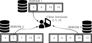
Figure 16: An illustration of a balanced combinatorial patterned-batch code with a minimum total storage overhead (no redundancy), which is spread out evenly among three servers. The set of nodes at each server corresponds to tree nodes in a color class of a balanced ancestral coloring of $T(3)$ as given in Fig. 3. A client only needs to download one item from each server for any batch request following a root-to-leaf-path pattern in $\mathcal{P}=\{\{2,4,8\}$, $\{2,4,9\}$, $\{2,5,10\}$, $\{2,5,11\}$, $\{3,6,12\}$, $\{3,6,13\}$, $\{3,7,14\}$, $\{3,7,15\}\}$.

Given a set of $N$ distinct nodes, an $(N,S,h,m)$ combinatorial batch code (CBC) provides a way to assign $S$ copies of nodes to $m$ different servers so that to retrieve a set of $h$ distinct nodes, a client can download at most one item from each server [45]. The goal is to minimize the total storage capacity required $S$. For instance, labelling $N=7$ nodes from 1 to 7, and use $m=5$ servers, an $(N=7,S=15,h=5,m=5)$ CBC allocates to five servers the sets $\{1,6,7\},\{2,6,7\},\{3,6,7\},\{4,6,7\},\{5,6,7\}$ (Paterson et al., [64]). One can verify that an arbitrary set of $h=5$ nodes can be retrieved by collecting one item from each set. Here, the storage requirement is $S=15>N=7$. It has been proved (see, e.g., [64]) that when $h=m$, the minimum possible $N$ is in the order of $\Theta(Nh)$, which implies that the average replication factor across $N$ nodes is $\Theta(h)$.

It turns out that $S=N$ (equivalently, replication factor one or no replication) is achievable if the $h$ retrieved nodes are not arbitrary and follow a special pattern. More specifically, if the $N$ nodes can be organised as nodes in a perfect binary tree $T(h)$ except the root and only sets of nodes along root-to-leaf paths (ignoring the root) are to be retrieved, then each item only needs to be stored in one server and requires no replication across different servers, which implies that $S=N$. A trivial solution is to use layer-based sets, i.e., Server $i$ stores nodes in Layer $i$ of the tree, $i=1,2,\ldots,h$. If we also want to balance the storage across the servers, that is, to make sure that the number of nodes assigned to every server differs from each other by at most one, then the layer-based solution no longer works and a balanced ancestral coloring of the tree nodes (except the root) will be required (see Fig. 16 for an example). We refer to this kind of code as balanced combinatorial patterned-batch codes. The balance requirement can also be generalized to the heterogeneous setting in which different servers may have different storage capacities. It is an intriguing open problem to discover other patterns (apart from the root-to-leaf paths considered in this paper) so that (balanced or heterogeneous) combinatorial patterned-batch codes with optimal total storage capacity $S=N$ exist.

Appendix G Connection to Equitable Colorings.

By finding balanced ancestral colorings of perfect binary trees, we are also able to determine the equitable chromatic number of a new family of graphs.

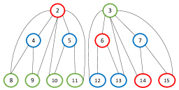
Figure 17: An equitable coloring of $T^{\prime}(3)$ using three colors (Red, Green, and Blue). The graph $T^{\prime}(3)$ is a disconnected graph obtained from $T(3)$ by first removing its root and then by adding edges between every node and all of its descendants.

An undirected graph $G$ (connected or not) is said to be equitable $k$-colorable if its vertices can be colored with $k$ colors such that no adjacent vertices have the same color and moreover, the sizes of the color classes differ by at most one [65]. The equitable chromatic number $\chi_{=}(G)$ is the smallest integer $k$ such that $G$ is equitable $k$-colorable. There has been extensive research in the literature on the equitable coloring of graphs (see, for instance, [66], for a survey), noticeably, on the Equitable Coloring Conjecture, which states that for a connected graph $G$ that is neither a complete graph nor an odd cycle, then $\chi_{=}(G)\leq\Delta(G)$, where $\Delta(G)$ is the maximum degree of a vertex in $G$. Special families of graphs that support the Equitable Coloring Conjecture include trees, bipartite graphs, planar and outerplanar graphs, among others.

The existence of balanced ancestral colorings of the perfect binary tree $T(h)$ established in this work immediately implies that $\chi_{=}(T^{\prime}(h))\leq h$, where $T^{\prime}(h)$ is a disconnected graph obtained from $T(h)$ by first removing its root and then by adding edges between every node $u$ and all of its descendants (see Fig. 17 for a toy example of $T^{\prime}(3)$). Note that $T^{\prime}(h)$ is neither a tree, a bipartite graph, a planar graph, nor an outerplanar graph for $h\geq 5$ (because it contains the complete graph $K_{h}$ as a subgraph). On top of that, it is not even connected and so the Equitable Coloring Conjecture doesn’t apply (and even if it applied, the maximum vertex degree is $\Delta(T^{\prime}(h))=2^{h}-2$, which is very far from $h$ and therefore would give a very loose bound). Furthermore, as $h$ nodes along a path from node 2 (or 3) to a leaf are ancestors or descendants of each other (hence forming a complete subgraph $K_{h}$), they should all belong to different color classes, which implies that $\chi_{=}(T^{\prime}(h))\geq h$. Thus, $\chi_{=}(T^{\prime}(h))=h$. Moreover, a balanced ancestral coloring of $T(h)$ provides an equitable $h$-coloring of $T^{\prime}(h)$. To the best of our knowledge, the equitable chromatic number of this family of graphs has never been discovered before.

We continue the discussion of the connections with the theory of majorization, e.g., on vertex coloring of claw-free graphs [67] and edge coloring [68] as below.

Appendix H Connection to the Theory of Majorization

We discuss below the connection of some of our results to the theory of majorization [69].

Definition 8 (Majorization).

For two vectors $\vec{x}=[x_{1},\ldots,x_{h}]$ and $\vec{y}=[y_{1},\ldots,y_{h}]$ in $\mathbb{R}^{h}$ with $x_{1}\geq\ldots\geq x_{h}$ and $y_{1}\geq\ldots\geq y_{h}$, $\vec{y}$ majorizes $\vec{x}$, denoted by $\vec{x}\prec\vec{y}$, if the following conditions hold.

• $\sum_{i=1}^{\ell}y_{i}\geq\sum_{i=1}^{\ell}x_{i}$, for every $1\leq\ell\leq h$, and

• $\sum_{i=1}^{h}y_{i}=\sum_{i=1}^{h}x_{i}$.

Equivalently, when $\vec{x}$ and $\vec{y}$ are sorted in non-decreasing order, i.e., $x_{1}\leq\ldots\leq x_{h}$ and $y_{1}\leq\ldots\leq y_{h}$, $\vec{x}\prec\vec{y}$ if the following conditions hold.

• $\sum_{i=1}^{\ell}y_{i}\leq\sum_{i=1}^{\ell}x_{i}$, for every $1\leq\ell\leq h$, and

• $\sum_{i=1}^{h}y_{i}=\sum_{i=1}^{h}x_{i}$.

Now, let $\vec{c}_{h}=[2,2^{2},\ldots,2^{h}]$. Clearly, $\vec{c}$ is $h$-feasible (according to Definition 6) if and only if all elements of $\vec{c}$ are integers and $\vec{c}\prec\vec{c}_{h}$. From the perspective of majorization, we now reexamine some of our results and make connections with existing related works.

First, Theorem 2 states that $T(h)$ is ancestral $\vec{c}$-colorable if and only if $\vec{c}\prec\vec{c}_{h}$. Note that it is trivial that $T(h)$ is ancestral $\vec{c}_{h}$-colorable (one color for each layer). Equivalently, $T^{\prime}(h)$, which is obtained from $T(h)$ by adding edges between each node and all of its descendants, is $\vec{c}_{h}$-colorable (i.e., it can be colored using $c_{i}$ Color $i$ so that adjacent vertices have different colors). A result similar to Theorem 2 was proved by Folkman and Fulkerson [68] but for the edge coloring problem for a general graph, which states that if a graph $G$ is $\vec{c}$-colorable and $\vec{c^{\prime}}\prec\vec{c}$ then $G$ is also $\vec{c^{\prime}}$-colorable. However, the technique used in [68] for edge coloring doesn’t work in the context of vertex coloring, which turns out to be much more complicated. The same conclusion for vertex coloring, as far as we know, only holds for claw-free graphs (see de Werra [67], and also [66, Theorem 4]). Recall that a claw-free graph is a graph that doesn’t have $K_{1,3}$ as an induced subgraph. However, our graph $T^{\prime}(h)$ contains a claw when $h\geq 3$, e.g., the subgraph induced by Nodes 2, 4, 10, and 11 (see Fig. 17). Therefore, this result doesn’t cover our case.

Second, in the language of majorization, the Color-Splitting Algorithm starts from an integer vector $\vec{c}$ of dimension $h$ that is majorized by $\vec{c}_{h}$ and creates two new integer vectors, both of dimension $h-1$ and majorized by $\vec{c}_{h-1}$. Applying the algorithm recursively produces $2^{h-1}$ sequences of vectors (of decreasing dimensions) where the $i$th element in each sequence is majorized by $\vec{c}_{h-i+1}$.

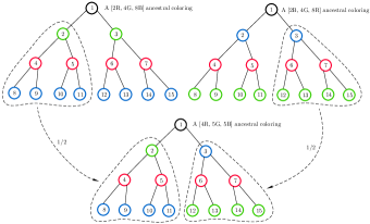
Figure 18: A [4R, 5G, 5B] ancestral coloring for $T_{3}$ can be obtained by “stitching” one half of the [4R, 2G, 8B] (trivial) coloring and one half of the [4R, 8G, 2B] (trivial) coloring. Note that $[4,5,5]=\frac{1}{2}[4,2,8]+\frac{1}{2}[4,8,2]$.

In the remainder of this section, we discuss a potential way to solve the ancestral tree coloring problem using a geometric approach. It was proved by Hardy, Littlewood, and Pólya in 1929 that $\vec{x}\prec\vec{y}$ if and only if $\vec{x}=\vec{y}P$ for some doubly stochastic matrix $P$. Moreover, the Birkhoff theorem ensures that every doubly stochastic matrix can be expressed as a convex combination of permutation matrices. With these, a geometric interpretation of majorization was established that $\vec{x}\prec\vec{y}$ if and only if $\vec{x}$ lies in the convex hull of all the permutations of $\vec{y}$ [69]. Therefore, it is natural to consider a geometric approach to the ancestral coloring problem. The following example is one such attempt.

Example 5.

Let $h=3$. Recall that $\vec{c}_{h}=[2,4,8]$. Also, let $\vec{c^{\prime}}=[4,5,5]$ and $\vec{c^{\prime\prime}}=[3,4,7]$. Clearly, $\vec{c^{\prime}}\prec\vec{c}_{h}$ and $\vec{c^{\prime\prime}}\prec\vec{c}_{h}$, and hence the CSA would work for both cases. Alternatively, we first write $\vec{c^{\prime}}$ and $\vec{c^{\prime\prime}}$ as convex combinations of permutations of $\vec{c}_{h}$ as

$$\vec{c^{\prime}} =\frac{1}{2}[4,2,8]+\frac{1}{2}[4,8,2],$$ (17)

$$\vec{c^{\prime\prime}} =\frac{1}{4}[2,4,8]+\frac{1}{4}[2,8,4]+\frac{1}{2}[4,2,8].$$ (18)

Note that every permutation of $\vec{c}_{h}$ admits a trivial layer-based ancestral coloring as shown in the two trees at the top in Fig. 18. Now, (17) demonstrates that it is possible to obtain an ancestral coloring for $\vec{c^{\prime}}$ by taking a half of the tree colored by $[4,2,8]$ and a half of that colored by $[4,8,2]$ and stitching them together, which is precisely what we illustrate in Fig. 18. Similarly, Fig. 19 shows how we obtain an ancestral coloring for $\vec{c^{\prime\prime}}=[3,4,7]$ by taking a quarter of the tree colored by $[2,4,8]$, a quarter of the tree colored by $[2,8,4]$, and a half of the tree colored by $[4,2,8]$ and stitching them together.

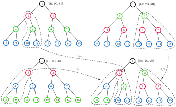
Figure 19: A [3R, 4G, 7B] ancestral coloring for $T_{3}$ can be obtained by “stitching” a quarter of the coloring [2R, 4G, 8B], a quarter of the coloring [2R, 8G, 4B], and a half of the coloring [4R, 2G, 8B]. Note that $[3,4,7]=\frac{1}{4}[2,4,8]+\frac{1}{4}[2,8,4]+\frac{1}{2}[4,2,8]$.

With the success of this approach for the above examples ($h=3$) and other examples with $h=4$ (not included for the sake of conciseness), it is tempting to believe that for every $\vec{c}$ majorized by $\vec{c}_{h}$, an ancestral coloring can be obtained by stitching sub-trees of trivial layer-based ancestral-colored trees. However, our initial (failed) attempt for $h=5$ indicates that it could be quite challenging to obtain ancestral colorings by such a method, even if a convex and dyadic combination can be identified. Further investigation on this direction is left for future work.

References

- [1] R. C. Merkle, “A digital signature based on a conventional encryption function,” in Proceedings of the Conference on the Theory and Application of Cryptographic Techniques (EUROCRYPT). Springer, 1987, pp. 369–378.
- [2] G. DeCandia, D. Hastorun, M. Jampani, G. Kakulapati, A. Lakshman, A. Pilchin, S. Sivasubramanian, P. Vosshall, and W. Vogels, “Dynamo: Amazon’s highly available key-value store,” ACM SIGOPS Operating Systems Review, vol. 41, no. 6, pp. 205–220, 2007.
- [3] G. C. Transparency. How CT works: How CT fits into the wider Web PKI ecosystem. [Online]. Available: https://certificate.transparency.dev/howctworks/
- [4] S. Nakamoto, “Bitcoin: A peer-to-peer electronic cash system,” Decentralized Business Review, 2008.
- [5] D. G. Wood, “Ethereum: A secure decentralised generalised transaction ledger,” Ethereum project (yellow paper), vol. 151, no. 2014, pp. 1–32, 2014.
- [6] J. B. Bernabe, J. L. Canovas, J. L. Hernandez-Ramos, R. T. Moreno, and A. Skarmeta, “Privacy-preserving solutions for blockchain: Review and challenges,” IEEE Access, vol. 7, pp. 164 908–164 940, 2019.
- [7] M. Raikwar, D. Gligoroski, and K. Kralevska, “Sok of used cryptography in blockchain,” IEEE Access, vol. 7, pp. 148 550–148 575, 2019.
- [8] G. Almashaqbeh and R. Solomon, “SoK: Privacy-preserving computing in the blockchain era,” in In Proceedings of the IEEE European Symposium on Security and Privacy (EuroS&P), 2022, pp. 124–139.
- [9] Google. Google’s Certificate Transparency Project. [Online]. Available: https://certificate.transparency.dev/
- [10] W. Lueks and I. Goldberg, “Sublinear scaling for multi-client private information retrieval,” in Proceedings of the 19th International Conference on Financial Cryptography and Data Security, 2015, pp. 168–186.
- [11] D. Kales, O. Omolola, and S. Ramacher, “Revisiting user privacy for certificate transparency,” in Proceedings of the IEEE European Symposium on Security and Privacy (EuroS&P), 2019, pp. 432–447.
- [12] B. Chor, O. Goldreich, E. Kushilevitz, and M. Sudan, “Private information retrieval,” in Proceedings of the IEEE Symposium on Foundations of Computer Science (FOCS), 1995, pp. 41–50.
- [13] E. Kushilevitz and R. Ostrovsky, “Replication is not needed: Single database, computationally-private information retrieval,” in Proceedings of the 38th IEEE Symposium on Foundations of Computer Science (FOCS), 1997, pp. 364–373.
- [14] A. Beimel and Y. Ishai, “Information-theoretic private information retrieval: A unified construction,” in Proceedings of the 28th International Colloquium on Automata, Languages and Programming, 2001, pp. 912–926.
- [15] D. Woodruff and S. Yekhanin, “A geometric approach to information-theoretic private information retrieval,” in Proceedings of the 20th Annual IEEE Conference on Computational Complexity (CCC’05), 2005, pp. 275–284.
- [16] C. Cachin, S. Micali, and M. Stadler, “Computationally private information retrieval with polylogarithmic communication,” in Proceedings of the International Conference on the Theory and Application of Cryptographic Techniques (EUROCRYPT), 1999, pp. 402–414.
- [17] C. A. Melchor, J. Barrier, L. Fousse, and M.-O. Killijian, “XPIR: Private information retrieval for everyone,” Proceedings on Privacy Enhancing Technologies, pp. 155–174, 2016.
- [18] S. Angel, H. Chen, K. Laine, and S. Setty, “PIR with compressed queries and amortized query processing,” in Proceedings of the IEEE symposium on security and privacy (S&P), 2018, pp. 962–979.
- [19] H. Corrigan-Gibbs and D. Kogan, “Private information retrieval with sublinear online time,” in Proceedings of the 39th Annual International Conference on the Theory and Applications of Cryptographic Techniques (EUROCRYPT), 2020, pp. 44–75.
- [20] A. Davidson, G. Pestana, and S. Celi, “FrodoPIR: Simple, scalable, single-server private information retrieval,” in Proceedings on Privacy Enhancing Technologies, 2022.
- [21] H. Sun and S. A. Jafar, “The capacity of private information retrieval,” IEEE Transactions on Information Theory, vol. 63, no. 7, pp. 4075–4088, 2017.
- [22] K. Banawan and S. Ulukus, “Multi-message private information retrieval: Capacity results and near-optimal schemes,” IEEE Transactions on Information Theory, vol. 64, pp. 6842–6862, 2018.
- [23] E. Y. Yang, J. Xu, and K. H. Bennett, “Private information retrieval in the presence of malicious failures,” in Proceedings of the 26th Annual International Computer Software and Applications, 2002, pp. 805–810.
- [24] A. Beimel and Y. Stahl, “Robust information-theoretic private information retrieval,” in Proceedings of the Third International Conference on Security in Communication Networks, 2003, pp. 326–341.
- [25] ——, “Robust information-theoretic private information retrieval,” Journal of Cryptology, vol. 20, pp. 295–321, 2007.
- [26] I. Goldberg, “Improving the robustness of private information retrieval,” in 2007 IEEE Symposium on Security and Privacy (SP’07). IEEE, 2007, pp. 131–148.
- [27] C. Devet, I. Goldberg, and N. Heninger, “Optimally robust private information retrieval,” in Proceedings of the USENIX Security Symposium, 2012, pp. 269–283.
- [28] L. Zhao, X. Wang, and X. Huang, “Verifiable single-server private information retrieval from lwe with binary errors,” Information Sciences, vol. 546, pp. 897–923, 2021.
- [29] L. Zhu, C. Lin, F. Lin, and L. F. Zhang, “Post-quantum cheating detectable private information retrieval,” in Proceedings of the IFIP International Conference on ICT Systems Security and Privacy Protection. Springer, 2022, pp. 431–448.
- [30] P. Ke and L. F. Zhang, “Two-server private information retrieval with result verification,” in Proceedings of the IEEE International Symposium on Information Theory (ISIT), 2022, pp. 408–413.
- [31] ——, “Private information retrieval with result verification for more servers,” in Proceedings of the International Conference on Applied Cryptography and Network Security (ANCS), 2023, pp. 197–216.
- [32] L. F. Zhang and H. Wang, “Multi-server verifiable computation of low-degree polynomials,” in Proceedings of the IEEE Symposium on Security and Privacy (S&P), 2022, pp. 596–613.
- [33] S. Ben-David, Y. T. Kalai, and O. Paneth, “Verifiable private information retrieval,” in Proceedings of the Theory of Cryptography Conference, 2022, pp. 3–32.
- [34] S. Colombo, K. Nikitin, H. Corrigan-Gibbs, D. J. Wu, and B. Ford, “Authenticated private information retrieval,” in Proceedings of the 32nd USENIX Security Symposium, 2023.
- [35] Q. Cao, H. Y. Tran, S. H. Dau, X. Yi, E. Viterbo, C. Feng, Y.-C. Huang, J. Zhu, S. Kruglik, and H. M. Kiah, “Committed private information retrieval,” in Proceedings of the European Symposium on Research in Computer Security, 2023, accepted.
- [36] S. Kruglik, S. H. Dau, H. M. Kiah, and H. Wang, “-server byzantine-resistant PIR scheme with optimal download rate and optimal file size,” in Proceedings of the IEEE International Symposium on Information Theory (ISIT), 2023, accepted.
- [37] ——, “Two-server private information retrieval with optimized download rate and result verification,” in Proceedings of the IEEE International Symposium on Information Theory (ISIT), 2023, accepted.
- [38] Microsoft. SealPIR: A computational PIR library that achieves low communication costs and high performance. [Online]. Available: https://github.com/microsoft/SealPIR
- [39] K. D. Albab, R. Issa, M. Varia, and K. Graffi, “Batched differentially private information retrieval,” in 31st USENIX Security Symposium (USENIX Security 22), 2022, pp. 3327–3344.
- [40] NIST. Hash functions. [Online]. Available: https://csrc.nist.gov/projects/hash-functions
- [41] A. Ali, T. Lepoint, S. Patel, M. Raykova, P. Schoppmann, K. Seth, and K. Yeo, “Communication-computation trade-offs in PIR,” in In Proceedings of the 30th USENIX Security Symposium, 2021, pp. 1811–1828.
- [42] M. H. Mughees and L. Ren, “Vectorized batch private information retrieval,” in 2023 IEEE Symposium on Security and Privacy (S&P), 2023.
- [43] S. Angel and S. Setty, “Unobservable communication over fully untrusted infrastructure,” in Proceedings of the 12th USENIX Conference on Operating Systems Design and Implementation, ser. OSDI’16, 2016, pp. 551––569.
- [44] B. H. Bloom, “Space/time trade-offs in hash coding with allowable errors,” Communications of the ACM, vol. 13, no. 7, pp. 422–426, 1970.
- [45] Y. Ishai, E. Kushilevitz, R. Ostrovsky, and A. Sahai, “Batch codes and their applications,” in Proceedings of the thirty-sixth Annual ACM Symposium on Theory of computing, 2004, pp. 262–271.
- [46] D. Stinson, R. Wei, and M. B. Paterson, “Combinatorial batch codes,” Advances in Mathematics of Communications, vol. 3, no. 1, pp. 13–27, 2009.
- [47] A. S. Rawat, Z. Song, A. G. Dimakis, and A. Gál, “Batch codes through dense graphs without short cycles,” IEEE Transactions on Information Theory, vol. 62, no. 4, pp. 1592–1604, 2016.
- [48] S. Angel and S. Setty, “Unobservable communication over fully untrusted infrastructure,” in Proceedings of the USENIX Symposium on Operating Systems Design and Implementation (OSDI), 2016, pp. 551–569.
- [49] C. Balbuena, “A construction of small regular bipartite graphs of girth 8,” Discrete Mathematics and Theoretical Computer Science, vol. 11, no. 2, pp. 33–46, 2009.
- [50] R. Pagh and F. F. Rodler, “Cuckoo hashing,” Journal of Algorithms, vol. 51, no. 2, pp. 122–144, 2004.
- [51] V. Strassen et al., “Gaussian elimination is not optimal,” Numerische mathematik, vol. 13, no. 4, pp. 354–356, 1969.
- [52] N. Gilboa and Y. Ishai, “Distributed point functions and their applications,” in In Proceedings of the 33rd Annual International Conference on the Theory and Applications of Cryptographic Techniques (EUROCRYPT), 2014, pp. 640–658.
- [53] E. Boyle, N. Gilboa, and Y. Ishai, “Function secret sharing,” in Proceedings of the Conference on the Theory and Application of Cryptographic Techniques (EUROCRYPT), 2015, pp. 337–367.
- [54] ——, “Function secret sharing: Improvements and extensions,” in Proceedings of the ACM SIGSAC Conference on Computer and Communications Security, 2016, pp. 1292–1303.
- [55] gRPC – An RPC library and framework. [Online]. Available: https://github.com/grpc/grpc
- [56] CSA code. [Online]. Available: https://github.com/PIR-PIXR/CSA-parallel-PIR
- [57] Blockchain.com Exchange APIs. [Online]. Available: https://www.blockchain.com/api
- [58] Cryptocurrency Statistics. [Online]. Available: https://bitinfocharts.com/
- [59] Google GSON. [Online]. Available: https://github.com/google/gson
- [60] Microsoft SEAL. [Online]. Available: https://github.com/microsoft/SEAL/tree/4.0.0
- [61] DP-PIR. [Online]. Available: https://github.com/multiparty/DP-PIR/tree/usenix2022
- [62] M. Charikar, V. Guruswami, R. Kumar, S. Rajagopalan, and A. Sahai, “Combinatorial feature selection problems,” in Proceedings of the IEEE Symposium on Foundations of Computer Science (FOCS), 2000, pp. 631–640.
- [63] Blockchain.com Exchange APIs. [Online]. Available: https://www.blockchain.com/api
- [64] M. B. Paterson, D. R. Stinson, and R. Wei, “Combinatorial batch codes,” Advances in Mathematics of Communications, vol. 3, no. 1, pp. 13–27, 2009.
- [65] W. Meyer, “Equitable coloring,” The American mathematical monthly, vol. 80, no. 8, pp. 920–922, 1973.
- [66] K.-W. Lih, Equitable Coloring of Graphs. New York, NY: Springer New York, 2013, pp. 1199–1248.
- [67] D. De Werra, “Some uses of hypergraphs in timetabling,” Asia-Pacific Journal of Operational Research, vol. 2, no. ARTICLE, pp. 2–12, 1985.
- [68] J. Folkman and D. Fulkerson, Edge colorings in bipartite graphs. Rand Corporation, 1966.
- [69] A. W. Marshall, Inequalities: Theory of Majorization and Its Applications, ser. Springer Series in Statistics. New York, NY: Springer New York, 2011.