Best of both worlds: Multi-task Audio-Visual Automatic Speech Recognition and Active Speaker Detection

Abstract

Under noisy conditions, automatic speech recognition (ASR) can greatly benefit from the addition of visual signals coming from a video of the speaker’s face. However, when multiple candidate speakers are visible this traditionally requires solving a separate problem, namely active speaker detection (ASD), which entails selecting at each moment in time which of the visible faces corresponds to the audio. Recent work has shown that we can solve both problems simultaneously by employing an attention mechanism over the competing video tracks of the speakers’ faces, at the cost of sacrificing some accuracy on active speaker detection. This work closes this gap in active speaker detection accuracy by presenting a single model that can be jointly trained with a multi-task loss. By combining the two tasks during training we reduce the ASD classification accuracy by approximately $25\%$, while simultaneously improving the ASR performance when compared to the multi-person baseline trained exclusively for ASR.

Index Terms—  Audio-visual automatic speech recognition, active speaker detection, speaker diarization, multi-task learning.

1 Introduction

Complementing the acoustic signal with a video of the speaker’s face is a useful strategy for ASR under noisy conditions [1, 2, 3, 4, 5, 6, 7]. In a realistic setting, however, multiple faces are potentially simultaneously on screen and one must decide which speaker face video to feed to the model. This first step has been traditionally treated as a separate problem [8, 9], but recent work has shown that we can obtain this association with an end-to-end model employing an attention mechanism over the candidate faces [10, 11].

As a side effect, this attention mechanism implicitly captures the correspondence between the audio and the video of the active speaker and, thus, can also be used as an active speaker detection (ASD) model in addition to ASR. However, while interesting in itself, despite having nontrivial accuracy, the implicit association doesn’t perform as well as when the attention is trained explicitly for active speaker detection (for a detailed study, see [11]). ASD essentially provides a strong signal for diarization, and high ASD accuracy as a side-product is a compelling reason to include the visual signal in ASR models. Having a single model or at least sharing the visual frontend between the two tasks is particularly important since video processing in the frontend is computationally expensive.

The present work closes this gap by addressing the following question: Can we get both high accuracy on active speaker detection (ASD) and low word error rate (WER) by training a single multi-person A/V ASR model in a multi-task setting? We present a multi-task learning (MTL) [12] setup for a model that can simultaneously perform audio-visual ASR and active speaker detection, improving previous work on multi-person audio-visual ASR. We show that combining the two tasks is enough to significantly improve the performance of the model in the ASD task relative to the baseline in [10, 11], while not degrading the ASR performance of the same model trained exclusively for ASR.

2 Model

Figure 1 shows an overview of our model, and we explain in detail each component next.

2.1 A/V Backbone: Shared Audio-Visual Frontend

Acoustic Features. We employ log mel filterbank features as input to our trainable models. The 16kHz audio is framed with 25ms windows smoothed with the Hann window function, with strides of 10ms between frames. We compute log mel filter bank features with 80 channels, and fold every 3 consecutive feature vectors together, yielding a 240-dimensional feature vector every 30ms ($\approx 33.3$Hz). The resulting acoustic features tensor will be denoted by ${\bm{\mathsfit{A}}}\in\mathbb{R}^{B\times T\times D_{a}}$, where $B$ is the batch size, $T$ is the number of time steps and $D_{a}$ ($=240$) the dimension of the acoustic features. During training, sequences of different lengths within a batch are zero-padded and limited to 512 steps.

Audio and Video Synchronization. Since the videos in our training set have frame rates ranging from around 23 to 30 fps, in order to make the input uniform we resample the videos in the temporal dimension to the acoustic features sample rate (33.3Hz). The resampling is performed with nearest neighbor interpolation. In the spatial dimension, we crop the full face tracks around the mouth region to generate images of resolution $128\times 128$, with RGB channels normalized between $-1$ and $1$.

Layer	Kernel	Output	Spatial	Normalization
	Size	Channels	Pooling?	Groups
0	[1, 3, 3]	23	True	1
1	[3, 1, 1]	64	False	32
2	[1, 3, 3]	64	True	1
3	[3, 1, 1]	128	False	32
4	[1, 3, 3]	256	True	1
5	[3, 1, 1]	256	False	32
6	[1, 3, 3]	921	False	1
7	[3, 1, 1]	512	False	32
8	[1, 3, 3]	460	True	1
9	[1, 1, 1]	512	False	32

Table 1: Configuration of (2+1)D ConvNet used to compute visual features. Max pooling is over a $2\times 2$ window on the spatial dimensions only. Additionally, we use a stride of 2 on both spatial dimensions on the first layer. For all layers, we use ‘VALID’ paddings in the spatial dimensions, and ‘SAME’ paddings on the temporal dimension.

Visual Features. For the visual frontend, we compute visual features ${\bm{\mathsfit{V}}}\in\mathbb{R}^{M\times T\times D_{v}}$ with a 10-layer (2+1)D ConvNet [13, 14] on top of the synchronized video, where $M$ is the number of competing face tracks and $D_{v}$, the dimension of the visual features. The exact parameters of the ConvNet can be found on Table 1. This is an important deviation from [11], where blocks of 3D convolutions were used instead. (2+1)D convolutions not only yield better performance, but are also less TPU memory intensive, allowing training with larger batch sizes, which has shown to be particularly important for obtaining lower word error rates. Note that each convolutional block is followed by group normalization [15], and the number of groups on each layer is indicated on the table.

Attention Mechanism. Visual features of competing faces are the slices ${\bm{\mathsfit{V}}}_{m,:,:}\in\mathbb{R}^{T\times D_{v}}$ along the first dimension of the visual features tensor. We employ an attention [16, 17] module in order to soft-select the one matching the audio. The attention queries ${\bm{\mathsfit{Q}}}\in\mathbb{R}^{B\times T\times D_{q}}$ are computed with a 1D ConvNet of 5 layers on top of the acoustic features (consult [10] for the exact parameters). We compute the attention scores with

$$S_{btm}=Q_{btq}W_{qv}V_{mtv},\quad\textrm{with}\quad{\bm{\mathsfit{S}}}\in\mathbb{R}^{B\times T\times M},$$ (1)

in Einstein summation notation, where ${\bm{\mathsfit{W}}}\in\mathbb{R}^{D_{q}\times D_{v}}$ is a trainable model parameter used for the bilinear function.

The attention scores are then normalized with a softmax function over the last dimension:

$$\alpha_{btm}=\frac{e^{S_{btm}}}{\sum_{l}e^{S_{btl}}},\quad\textrm{with}\quad\alpha\in\mathbb{R}^{B\times T\times M}.$$ (2)

which are then used to yield the attention weighted visual features corresponding to each audio query with the weighted sum

$$V^{\prime}_{btv}=\alpha_{btm}V_{mtv},\quad\textrm{with}\quad{\bm{\mathsfit{V}}}^{\prime}\in\mathbb{R}^{B\times T\times D_{v}}.$$ (3)

During training, we have matched pairs of audio and a single corresponding face track, so $M$ is equal to the batch size $B$. During inference, $B=1$ and $M$ is equal to the number of parallel face tracks in the video. The visual feature that is then fed to the ASR model consists of a soft average of all the face-specific visual features, with the largest weight being attributed to the face that most likely matches the audio”

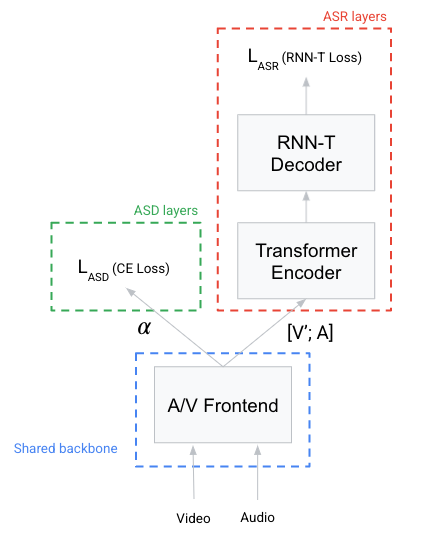
Fig. 1: Multi-task model for A/V ASR and ASD. $\alpha\in\mathbb{R}^{B\times T\times M}$ is the attention tensor, indicating the probability of each of the $M$ parallel video tracks being the active speaker for each of the $B$ audio queries and each timestep. ${\bm{\mathsfit{V}}}^{\prime}\in\mathbb{R}^{B\times T\times D_{v}}$ is the tensor with the attention weighted visual features, and ${\bm{\mathsfit{A}}}\in\mathbb{R}^{B\times T\times D_{a}}$ are the acoustic features.

2.2 ASR Model

For ASR, the weighted visual features and input acoustic features are then concatenated along the last dimension, producing audio-visual features ${\bm{\mathsfit{F}}}=[{\bm{\mathsfit{A}}};{\bm{\mathsfit{V}}}^{\prime}]\in\mathbb{R}^{B\times T\times(D_{a}+D_{v})}$, which are then fed to the ASR encoder.

Encoder. For ASR we use a 14 layer Transformer encoder [17]. Due to the quadratic complexity of attention over long sequences, we limit the attention context to 100 steps to the left and right of each timestep. We use 8 attention heads, each with dimension of 64, and a model dimension of 1024. This is another important improvement from [11], where a 6-layer BiLSTM encoder was used instead.

Decoder. We employ a standard RNN-T decoder [18, 19], with a stack of 2 LSTM layers of 2048 units and character tokens as input, with a vocabulary of size 128.

2.3 ASD Model

For ASD, the attention scores tensor ${\bm{\mathsfit{S}}}$ is used directly for the model prediction. For each audio query and each timestep, ${\bm{\mathsfit{S}}}$ gives a measure of how well each candidate video corresponds to the audio. During inference, the index of the selected video track is given by

$$I_{bt}=\operatorname*{arg\,max}_{m}S_{btm},\quad{\bm{\mathsfit{I}}}\in\mathbb{R}^{B\times T}.$$ (4)

3 Multi-Task Loss for A/V ASR and ASD

In this section, we describe how our model is trained by using a multi-task formulation to combine both ASR and ASD related losses.

ASD. For active speaker detection, the normalized attention weights $\alpha_{btm}$ can be used to train the attention module directly with cross entropy loss. Since during training we have pairs of corresponding audio and video from a single speaking face, we can write

$$L_{\textrm{ASD}}=\frac{1}{BT}\sum_{b=1}^{B}\sum_{t=1}^{T}\sum_{m=1}^{M}-[b=m]\log\alpha_{btm}.$$ (5)

ASR. During training, given (audio, video, transcript) triplets, we compute the ASR loss ($L_{\textrm{ASR}}$) with the RNN-T loss [18, 19]. RNN-T loss computes the negative log-loss of the target transcript by computing all possible input-output alignments with a forward-backward algorithm. For the sake of brevity, we refer the reader to [18, 19] for details.

MTL Loss. We combine the ASD and ASR losses with a weighted linear sum of the losses for each task:

$$L=\gamma L_{\textrm{ASR}}+(1-\gamma)L_{\textrm{ASD}},$$ (6)

where $0\leq\gamma\leq 1$ is a blending weight between the two loss functions. $\gamma=0$ corresponds to the model trained purely for ASD, while $\gamma=1$, purely for ASR.

Training. Given a value of $\gamma$, we initialize the training with a checkpoint from a model trained with a single video track for A/V ASR. We use the Adam optimizer [20] with a constant learning rate of $0.0002$ for 200k steps, and a batch size of 8 per TPU core.

4 Datasets

4.1 Training and Evaluation Data

Training. For training, we use over 90k hours of transcribed short YouTube video segments extracted with the semi-supervised procedure originally proposed in [21] and extended in [1, 22] to include video. We extract short segments where the force-aligned user uploaded transcription matches the transcriptions from a production quality ASR system. From these segments we then keep the ones in which the face tracks match the audio with high confidence. We refer the reader to [1, 22] for more details of the pipeline.

Evaluation. For the videos in both of our evaluation sets, we track the faces on screen and pick the segments with matching audio and video tracks with the same procedure used to extract the training data. Therefore, by design, the faces extracted from the video correspond with high probability to the speaker in the audio. We rely on two base datasets:

• YTDEV18 [1]: Composed of 25 hours of manually transcribed YouTube videos, not overlapping with the training set, containing around 20k utterances.

• LRS3-TED Talks [23]: This is the largest publicly available dataset for A/V ASR, so we evaluate on it as well for completeness.

4.2 Augmenting the Evaluation Sets with Parallel Video Tracks and Noise

In order to evaluate our model in the scenario where multiple face tracks are simultaneously visible in a video, we construct a new evaluation dataset as follows: On the single track evaluation sets described in the previous section, at time $t$ both the acoustic and visual features from the corresponding face are available. To build a dataset with $N$ parallel face tracks we start from the single track set, and for every pair of matched audio and face video track we randomly pick other $N-1$ face tracks from the same dataset. Therefore, during evaluation at each time step we have the acoustic features computed from the audio and $N$ candidate visual features, without knowing which one matches the audio. We generate separate datasets for $N=1,2,4,8$ to simulate a scenario where multiple on-screen faces are competing with the face of the target speaker.

Moreover, in order to measure the impact of the visual modality, we also evaluate on noisy conditions by adding babble noise randomly selected from the NoiseX dataset [24] at 0dB, 10dB and 20dB to each utterance.

Table 2: Top-1 Face track selection accuracy at the frame level (ACC) and word error rate (WER) for the various noise levels, number of competing face tracks, and loss weights $\gamma$. $\gamma=0.0$ corresponds to a model trained only with ASD loss, while $\gamma=1.0$, only with ASR loss.

Dataset	Noise	Tracks	$\gamma$										Audio Only	1-Track A/V
			0.0		0.25		0.5		0.75		1.0
			ACC	WER	ACC	WER	ACC	WER	ACC	WER	ACC	WER	WER	WER
YTDEV18		1	1.00	–	1.00	13.17	1.00	13.01	1.00	13.12	1.00	12.92		13.09
		2	0.99	–	0.99	13.19	0.98	13.03	0.97	13.16	0.89	12.98	13.62	–
		4	0.98	–	0.97	13.23	0.96	13.03	0.93	13.19	0.77	13.15		–
		8	0.95	–	0.94	13.24	0.92	13.13	0.88	13.29	0.64	13.26		–
	20dB	1	1.00	–	1.00	13.30	1.00	13.23	1.00	13.30	1.00	13.14		13.24
		2	0.99	–	0.98	13.34	0.98	13.27	0.97	13.34	0.89	13.17	13.97	–
		4	0.97	–	0.96	13.38	0.95	13.32	0.93	13.41	0.77	13.33		–
		8	0.95	–	0.93	13.40	0.91	13.34	0.87	13.49	0.64	13.56		–
	10dB	1	1.00	–	1.00	14.42	1.00	14.42	1.00	14.56	1.00	14.38		14.32
		2	0.98	–	0.98	14.48	0.97	14.44	0.95	14.62	0.87	14.51	16.34	–
		4	0.96	–	0.94	14.60	0.93	14.59	0.90	14.72	0.74	14.93		–
		8	0.92	–	0.90	14.78	0.87	14.70	0.82	14.96	0.61	15.53		–
	0dB	1	1.00	–	1.00	22.58	1.00	22.59	1.00	23.04	1.00	23.57		21.33
		2	0.92	–	0.91	23.72	0.89	23.64	0.87	24.24	0.79	25.11	36.63	–
		4	0.84	–	0.81	25.61	0.79	25.27	0.73	26.19	0.61	28.94		–
		8	0.75	–	0.71	27.78	0.68	27.63	0.61	28.98	0.47	34.00		–
TED.LRS3		1	1.00	–	1.00	3.19	1.00	3.10	1.00	2.89	1.00	2.96		2.97
		2	0.99	–	0.98	3.18	0.97	3.13	0.97	2.89	0.92	2.96	3.45	–
		4	0.96	–	0.96	3.20	0.93	3.13	0.93	2.88	0.82	2.94		–
		8	0.93	–	0.92	3.16	0.88	3.16	0.86	2.96	0.70	3.18		–

5 Results

We train separate models with different blending weights $\gamma$ between the loss functions, and evaluate for both ASD and ASR tasks. The results are summarized on Table 2. $\gamma=0$ corresponds to a model trained purely for active speaker detection, and, thus, serves as an upper bound to the accuracy we can hope to achieve on the ASD task for the multi-task model. On the other extreme, $\gamma=1$ corresponds to a model trained purely with ASR loss, where the A/V attention frontend provides an ASD signal, despite not being optimized for an ASD task, similar to the work in [10, 11].

Additionally, we include the WERs for two baseline models on the two rightmost columns of Table 2: for a model trained only with audio, and for another trained with a single video track of the speaker always matching the audio. The former serves as an upper bound to the WER we need to achieve with an A/V ASR model, since once the WER surpasses the audio-only level, including the video on an ASR model becomes unjustified.

Analysis. We clearly closed the gap on ASD by combining the two losses. For $\gamma<1.0$, there’s a clear improvement on all models in terms of ASD accuracy when compared to the baseline model ($\gamma=1$). For instance, with $\gamma=0.5$ we see a relative improvement on average at clean, 20dB, 10dB and 0dB of approximately $26\%$, $25\%$, $26\%$ and $29\%$ in relation to the baseline multi-track model from [11] (corresponding to $\gamma=1$ on the table above). When compared to the pure ASD baseline ($\gamma=0$), our new model shows a relative average degradation of only $2.1\%$, $2.5\%$, $3.3\%$ and $6.6\%$ in accuracy at the same noise levels, which is significantly lower than the degradations of the pure ASR model baseline ($\gamma=1$) from  [11] ($21.3\%$, $21.1\%$, $22.6\%$ and $26.2\%$ at clean, 20dB, 10dB and 0dB). Similarly, on TED.LRS3, with $\gamma=0.75$, we see an improvement of $13.9\%$, $18.1\%$ and $22.9\%$ in ASD accuracy in relation to the baseline from [11] ($\gamma=1$), while also slightly improving the ASR WER.

For ASR, not only we do not observe a significant degradation in WER overall when combining the two losses, but, on the contrary, the auxiliary ASD loss seems to help the ASR training, actually lowering the WER in most scenarios. For instance, with $\gamma=0.5$, we have a relative increase in accuracy by $0.2\%$, $0.1\%$, $1.95\%$ and $10.4\%$ on average at each noise level, showing that combining the two losses is a clear advantage for both tasks, while being able to use a single model for both A/V ASR and ASD.

6 Conclusions

We introduced a multi-task training setup for an Audio-Visual model that is capable of simultaneously performing automatic speech recognition and active speaker detection. The proposed architecture is particularly interesting as it provides a diarization signal for on-screen speakers, without requiring an explicit diarization model. We significantly improved on the active speaker detection classification accuracy without degrading the ASR performance. Our experiments show that a joint loss increases the accuracy on the ASD task by around $26\%$ when compared to the baseline state-of-the-art multi-person A/V ASR model [11], while actually increasing the ASR performance of the same model up to around $10\%$ on noisy scenarios.

References

- [1] Takaki Makino, Hank Liao, Yannis Assael, Brendan Shillingford, Basilio Garcia, Otavio Braga, and Olivier Siohan, “Recurrent neural network transducer for audio-visual speech recognition,” ASRU, 2019.
- [2] Triantafyllos Afouras, Joon Son Chung, Andrew Senior, Oriol Vinyals, and Andrew Zisserman, “Deep audio-visual speech recognition,” IEEE Transactions on Pattern Analysis and Machine Intelligence, p. 1–1, 2018.
- [3] Joon Son Chung, Andrew Senior, Oriol Vinyals, and Andrew Zisserman, “Lip reading sentences in the wild,” 2017 IEEE Conference on Computer Vision and Pattern Recognition (CVPR), Jul 2017.
- [4] G. Potamianos, C. Neti, G. Gravier, A. Garg, and A. W. Senior, “Recent advances in the automatic recognition of audiovisual speech,” Proceedings of the IEEE, vol. 91, no. 9, pp. 1306–1326, 2003.
- [5] K. Saenko and K. Livescu, “An asynchronous dbn for audio-visual speech recognition,” in 2006 IEEE Spoken Language Technology Workshop, 2006, pp. 154–157.
- [6] Naomi Harte and Eoin Gillen, “Tcd-timit: An audio-visual corpus of continuous speech,” Multimedia, IEEE Transactions on, vol. 17, pp. 603–615, 05 2015.
- [7] Dmitriy Serdyuk, Otavio Braga, and Olivier Siohan, “Audio-visual speech recognition is worth 32x32x8 voxels,” CoRR, vol. abs/2109.09536, 2021.
- [8] Joon Son Chung and Andrew Zisserman, “Out of time: Automated lip sync in the wild,” in Workshop on Multi-view Lip-reading, ACCV, 2016, 03 2017, pp. 251–263.
- [9] Soo-Whan Chung, Joon Son Chung, and Hong-Goo Kang, “Perfect match: Improved cross-modal embeddings for audio-visual synchronisation,” ICASSP 2019 - 2019 IEEE International Conference on Acoustics, Speech and Signal Processing (ICASSP), May 2019.
- [10] O. Braga, T. Makino, O. Siohan, and H. Liao, “End-to-end multi-person audio/visual automatic speech recognition,” in ICASSP 2020 - 2020 IEEE International Conference on Acoustics, Speech and Signal Processing (ICASSP), 2020, pp. 6994–6998.
- [11] Otavio Braga and Olivier Siohan, “A closer look at audio-visual multi-person speech recognition and active speaker selection,” in ICASSP 2021 - 2021 IEEE International Conference on Acoustics, Speech and Signal Processing (ICASSP), 2021, pp. 6863–6867.
- [12] Richard Caruana, “Multitask learning: A knowledge-based source of inductive bias,” in Proceedings of the Tenth International Conference on Machine Learning. 1993, pp. 41–48, Morgan Kaufmann.
- [13] Yann Lecun, Léon Bottou, Yoshua Bengio, and Patrick Haffner, “Gradient-based learning applied to document recognition,” in Proceedings of the IEEE, 1998, pp. 2278–2324.
- [14] Du Tran, Heng Wang, Lorenzo Torresani, Jamie Ray, Yann LeCun, and Manohar Paluri, “A closer look at spatiotemporal convolutions for action recognition,” 06 2018, pp. 6450–6459.
- [15] Yuxin Wu and Kaiming He, “Group normalization,” in Proceedings of the European Conference on Computer Vision (ECCV), 2018, pp. 3–19.
- [16] Dzmitry Bahdanau, Kyunghyun Cho, and Yoshua Bengio, “Neural machine translation by jointly learning to align and translate,” in 3rd International Conference on Learning Representations, ICLR 2015, San Diego, CA, USA, May 7-9, 2015, Conference Track Proceedings, 2015.
- [17] Ashish Vaswani, Noam Shazeer, Niki Parmar, Jakob Uszkoreit, Llion Jones, Aidan N Gomez, Lukasz Kaiser, and Illia Polosukhin, “Attention is all you need,” in Advances in neural information processing systems, 2017, pp. 5998–6008.
- [18] Alex Graves, “Sequence transduction with recurrent neural networks,” ICML, 2012.
- [19] Alex Graves, Abdel-rahman Mohamed, and Geoffrey Hinton, “Speech recognition with deep recurrent neural networks,” in 2013 IEEE international conference on acoustics, speech and signal processing. IEEE, 2013, pp. 6645–6649.
- [20] Diederik P. Kingma and Jimmy Ba, “Adam: A method for stochastic optimization,” in 3rd International Conference on Learning Representations, ICLR 2015, San Diego, CA, USA, May 7-9, 2015, Conference Track Proceedings, Yoshua Bengio and Yann LeCun, Eds., 2015.
- [21] H. Liao, E. McDermott, and A. Senior, “Large scale deep neural network acoustic modeling with semi-supervised training data for youtube video transcription,” in 2013 IEEE Workshop on Automatic Speech Recognition and Understanding, 2013, pp. 368–373.
- [22] Brendan Shillingford, Yannis Assael, Matthew W. Hoffman, Thomas Paine, Cían Hughes, Utsav Prabhu, Hank Liao, Hasim Sak, Kanishka Rao, Lorrayne Bennett, and et al., “Large-scale visual speech recognition,” Interspeech 2019, Sep 2019.
- [23] T. Afouras, J. S. Chung, and A. Zisserman, “Lrs3-ted: a large-scale dataset for visual speech recognition,” in arXiv preprint arXiv:1809.00496, 2018.
- [24] Andrew Varga and Herman J. M. Steeneken, “Assessment for automatic speech recognition: Ii. noisex-92: A database and an experiment to study the effect of additive noise on speech recognition systems,” Speech Communication, vol. 12, pp. 247–251, 1993.