Accelerating Real-Time Coupled Cluster Methods with Single-Precision Arithmetic and Adaptive Numerical Integration

Abstract

We explore the framework of a real-time coupled cluster method with a focus on improving its computational efficiency. Propagation of the wave function via the time-dependent Schrödinger equation places high demands on computing resources, particularly for high level theories such as coupled cluster with polynomial scaling. Similar to earlier investigations of coupled cluster properties, we demonstrate that the use of single-precision arithmetic reduces both the storage and multiplicative costs of the real-time simulation by approximately a factor of two with no significant impact on the resulting UV/vis absorption spectrum computed via the Fourier transform of the time-dependent dipole moment. Additional speedups — of up to a factor of 14 in test simulations of water clusters — are obtained via a straightforward GPU-based implementation as compared to conventional CPU calculations. We also find that further performance optimization is accessible through sagacious selection of numerical integration algorithms, and the adaptive methods, such as the Cash-Karp integrator provide an effective balance between computing costs and numerical stability. Finally, we demonstrate that a simple mixed-step integrator based on the conventional fourth-order Runge-Kutta approach is capable of stable propagations even for strong external fields, provided the time step is appropriately adapted to the duration of the laser pulse with only minimal computational overhead.

1 Introduction

Although quantum chemical models for the properties of stationary states have seen great advances over the last 60 years, both in terms of accuracy and computational efficiency, the non-equilibrium character of time-dependent Hamiltonians (e.g., in the presence of an external, oscillating electromagnetic field) requires approaches based on the time-dependent Schrödinger equation.^{1, 2, 3} While the most common techniques take a perturbational approach and treat spectroscopic responses in the frequency domain, thereby carefully avoiding the often-expensive time-propagation of the wave function, explicitly time-dependent methods have a number of important advantages over their perturbative counterparts. First, time-dependent methods allow straightforward connections to experimental conditions, such as fine-tuning the shape, duration, and intensity of the external fields. Second, such methods yield spectroscopic properties across a wide range of frequencies via Fourier transformation of, e.g., the time-dependent electric-dipole moment, rather than a relatively narrow window of frequencies produced by response techniques. Third, with careful propagation algorithms, time-dependent methods can permit simulation of more intense external fields than perturbation theory approaches. Finally, the ample resources available from modern numerical mathematics and computer science may be brought to bear to improve the stability and efficiency of the time propagation itself.

To exploit these advantages, a wide range of real-time methods have been explored over the last 30 years based on a variety of approximate solutions to the electronic Schrödinger equation, including Hartree-Fock (HF)⁴, density-functional theory (DFT),^{5, 6} configuration interaction (CI),^{7, 8} and coupled-cluster (CC)^{9, 10, 11} approaches. Among these, real-time DFT (RT-DFT) is the most widely used for spectroscopic applications across a range of fields from biochemistry to solid state physics where the target systems are relatively large.^{12, 13, 14, 15, 16} The theory behind real-time methods is continuously under development, however, and the same shortcomings of systematic convergence and limited robustness that apply to ground-state density-functionals also apply to RT-DFT. This motivates researchers to investigate higher-level methods.

Real-time coupled cluster (RT-CC) methods, in particular, can achieve exceptionally high accuracy in many cases^{17, 18} and have been explored in the context of real-time simulations for some years.^{9, 19, 11, 20, 21, 10, 22, 23, 24, 25, 26, 27} However, RT-CC approaches also suffer from the same affliction as that of their time-independent counterparts, viz., high-degree polynomial scaling with the size of the molecular system. For ground-state coupled cluster theory, techniques such as local correlation, ^{28, 29, 30, 31, 32, 33, 34, 35} fragmentation,^{36, 37, 38, 39} tensor decomposition,^{40, 41, 42, 43, 44, 45} and others have been developed to permit applications to larger molecular systems than conventional implementations allow. However, while such methods are potentially transferable to the corresponding time-dependent approaches, they have yet to be exploited to reduce the computational cost of RT-CC.

In addition to the development of more compact representations of the time-dependent wave function, the construction of the differential equations that represent the time-dependency of the relevant properties, as well as the choice of numerical integration algorithm can substantially affect the efficiency and/or the stability of the calculation. For example, DePrince and Nascimento^{46, 10} introduced left and right coupled cluster dipole functions within the equation-of-motion (EOM-CC) framework for calculating accurate linear absorption spectra across a wide frequency range. They demonstrated that propagating either the left- or right-hand dipole functions yielded the same result, thus reducing the computational cost by a factor of two compared to propagating both left- and right-hand coupled cluster wave functions. In 2016, Lopata¹⁵ and coworkers accelerated RT-DFT calculations of broadband spectra by applying Padé approximants to the Fourier transforms. Note that they gained a five times shorter simulation time by obtaining rapid convergence of spectra from Padé approximants, while the technique has no dependence on the level of theory. In 2019, Pedersen and Kvaal¹⁹ reported symplectic integrators such as Gauss-Legendre can provide stable implementations across long propagation times even with relatively strong external fields. In subsequent work, Pedersen, Kvaal, and co-workers¹¹ used orbital-adaptive time-dependent coupled cluster doubles (OATDCCD) to improve the stability of their RT-CC implementation even when strong external fields result in a non-dominant electronic ground state. For the application to core excitation spectra, Bartlett and coworkers^{25, 26} compared time-independent (TI) EOM-CC and time-dependent (TD) EOM-CC — as well as contributions beyond the dipole approximation — and concluded that TD-EOM-CC can provide accurate spectra for both core and valance spectra. In addition, in 2021, Li, DePrince, and co-workers²⁷ applied the short iterative Lanczos integration to the time-dependent (TD) EOM-CC method for a more efficient calculation of K-edge spectra.

In this paper, we consider alternative numerical approaches aimed at reducing the cost of RT-CC calculations. In most quantum chemical programs, numerical parameters are typically computed and stored using binary representations translating to approximately 15 decimal digits of (double) precision. However, pioneering studies by Yasuda,⁴⁷ Martinez and co-workers,^{48, 49, 50} Aspuru-Guzik and co-workers,⁵¹ DePrince and Hammond,⁵² Asadchev and Gordon⁵³, and Krylov and co-workers⁵⁴ have demonstrated that single-precision arithmetic in which the binary representation supports ca. seven decimal digits, is sufficient — and more cost effective — for many applications. Based on the success of this previous work, we have explored the use of single-precision arithmetic in the context of RT-CC codes, particularly for the simulation of linear absorption. Additionally, we report a single-precision RT-CC implementation for which we obtain significant further speed-up utilizing the parallel architecture of graphical processing units (GPUs).

Finally, we explore a range of numerical integrators for solving the RT-CC differential equations for time-dependent properties. Generally, there are three main types of such integrators: explicit, adaptive (or embedded), and implicit. Explicit integrators are so named because they take into account only the output of the previous time step when calculating the results of the current step, whereas adaptive integrators can adjust the step size at each iteration with specialized algorithms to control the local error. Finally, implicit integrators take in account the outputs of both the previous step and the current step when determining the results for the next step, an approach that is often more expensive due to the required iterative algorithm. The Runge-Kutta (RK) family of integrators⁵⁵ includes all three types and is commonly used for solving the initial value problem associated with the Schrödinger equations-of-motion. We have built a library of RK integrators using all three types that are compatible with the RT-CC algorithm, and here we compare their performance. Moreover, inspired by conventional adaptive integrators, we examine a mixed-step-size formalism to customize the propagation on the fly, depending on whether the external field is on or off.

2 Theory

The quantum mechanical description of a molecule or material subjected to an external time-dependent electromagnetic field requires solution of the time-dependent Schrödinger equation (TDSE), which is given in atomic units as

$$\hat{H}|\Psi\rangle=i\frac{d}{dt}|\Psi\rangle,$$ (1)

where the Hamiltonian,

$$\hat{H}(t)=\hat{H}_{0}+\hat{V}(t),$$ (2)

includes the molecular components, $\hat{H}_{0}$, and the time-dependent potential, $\hat{V}(t)$. In the time-dependent coupled-cluster framework,^{46, 19, 35} we choose phase-isolated right- and left-hand wave functions, respectively,

$$|\Psi_{\rm CC}\rangle=e^{\hat{T}(t)}|0\rangle e^{i\epsilon(t)},$$ (3)

and

$$\langle\Psi_{\rm CC}|=\langle 0|\left(1+\hat{\Lambda}(t)\right)e^{-\hat{T}(t)}e^{-i\epsilon(t)}.$$ (4)

In these expressions, $|0\rangle$ is the single-determinant reference state, and $\hat{T}(t)$ and $\hat{\Lambda}(t)$ are second-quantized excitation and de-excitation operators, respectively, relative to $|0\rangle$. These operators are parametrized by time-dependent amplitudes that must be determined by propagating the TDSE, which, using the coupled-cluster form of the wave function, yields right- and left-hand forms, viz.,

$$\langle\mu|\bar{H}|0\rangle=i\frac{dt_{\mu}}{dt},$$ (5)

and

$$\langle 0|\left(1+\hat{\Lambda}\right)\left[\bar{H},\tau_{\mu}\right]|0\rangle=-i\frac{d\lambda_{\mu}}{dt},$$ (6)

where the index $\mu$ denotes an excited/substituted determinant, $\tau_{\mu}$ is a second-quantized operator that generates such a determinant from the reference, $|0\rangle$, and the similarity-transformed Hamiltonian,

$$\bar{H}=e^{-\hat{T}}\hat{H}e^{\hat{T}},$$ (7)

plays a central role in both the formal RT-CC equations and the algorithmic implementation.

2.1 Propagation of the RT-CC Equations

As mentioned in section 1, we propagate the CC wave function using the Runge-Kutta class of integrators, which are designed to solve the general initial-value problem (IVP),

$$\frac{dy}{dt}=f(t,y),\ \ \ \ y(t_{0})=y_{0},$$ (8)

where $y$ is the unknown vector function, which is propagated in each iteration beginning from $y_{0}$, and $f(t,y)$ carries the functional dependence. Runge-Kutta methods for solving this IVP have the general form,

$$y_{n+1}=y_{n}+h\sum_{i=1}^{s}b_{i}k_{ni},$$ (9)

where

$$k_{ni}=f(x_{n}+c_{i}h,y_{n}+h\sum_{j=1}^{i-1}a_{ij}k_{nj}).$$ (10)

In these expressions, $h$ is the (time) step size, and the $a_{ij}$, $b_{i}$, and $c_{i}$ coefficients define the particular integrator. These coefficients may be written in a matrix form called Butcher Tableau⁵⁶ as shown in Table. 1. The matrix is symmetric for explicit integrators and asymmetric for implicit integrators, and adaptive integrators require an additional line of coefficients.⁵⁷ Generally, an additional higher-order solution can be calculated, and the difference between the higher-order and lower-order solutions is used for adjusting the step size. More complicated algorithms have also been developed for dynamic simulations, higher-order differential equations, discontinuous initial-value problems, etc.^{58, 59}.

$c_{1}$	$a_{11}$	$a_{12}$	$\cdots$	$a_{1s}$
$c_{2}$	$a_{21}$	$a_{22}$	$\cdots$	$a_{2s}$
$\vdots$	$\vdots$		$\ddots$	$\vdots$
$c_{s}$	$a_{s1}$	$a_{s2}$	$\cdots$	$a_{s,s}$
	$b_{1}$	$b_{2}$	$\cdots$	$b_{s}$

Table 1: Butcher tableau for Runge-Kutta integrators

In the RT-CC approach, we cast the time-dependent coupled-cluster left- and right-hand amplitude expressions, Eqs. (5) and (6), into the form of Eq. (8) such that the $t_{\mu}$ and $\lambda_{\mu}$ amplitudes are collected into a single vector $y$. Thus, the left-hand sides of Eqs. (5) and (6) provide the specific form of $f(t,y)$. Given that these are simply the residual equations for the $t_{\mu}$ and $\lambda_{\mu}$ amplitudes in the time-independent case, the initial vector, $y_{0}$, is naturally taken to be the solutions of the ground-state $\hat{T}$ and $\hat{\Lambda}$ equations. Thus, all of the same algorithmic infrastructure used in efficient implementations of ground-state CC methods — spin-adaptation, intermediate factorizations, symmetry exploitation (e.g. using direct-product-decomposition⁶⁰), etc. — are readily applicable to the RT-CC approach. [NB: We choose to keep the underlying molecular orbitals from the Hartree-Fock self-consistent field procedure from responding to the field in order to allow direct comparison to conventional CC response and equation-of-motion (EOM-CC) results.]

2.2 Linear Absorption Spectra from RT-CC

In CC theory, as with other wave-function-based methods, properties of interest may be calculated by taking the expectation value of the corresponding operator, though the non-Hermitian nature of the CC similarity-transformed Hamiltonian in Eq. (7) leads to a generalized expectation value expression involving both the left- and right-hand CC wave functions. For example, the time-dependent, induced electric dipole moment may be computed at a given time step, $t_{k}$, as

$$\mu_{\alpha}(t_{k})=\langle 0|\left(1+\hat{\Lambda}(t_{k})\right)e^{-\hat{T}(t_{k})}\hat{\mu}_{\alpha}e^{\hat{T}(t_{k})}|0\rangle(t_{k})=\textrm{Tr}\left(\rho(t_{k})\cdot\hat{\mu}_{\alpha}\right)$$ (11)

where $\rho$ is the (unrelaxed) time-dependent one-particle density matrix and $\hat{\mu}_{\alpha}$ is the $\alpha$-th Cartesian component of the electric dipole operator.

If the perturbing potential is an electric field, i.e.,

$$V(t)=-\hat{\mu}_{\alpha}E_{\beta}(t),$$ (12)

then, to a first approximation, the induced dipole moment is related to the dipole polarizability as^{61, 62}

$$\mu_{\alpha}(t)=\alpha_{\alpha\beta}(t)\left(E_{\beta}(t)\right)_{0},$$ (13)

where $\alpha_{\alpha\beta}$ is the $\alpha,\beta-$th Cartesian component of the polarizability tensor, the subscript $0$ indicates that the field is taken at the origin, and we imply the Einstein summation convention over repeated indices. (We note that high-intensity fields will of course induce non-linear contributions to the induced-dipole, thus affecting the molecule’s spectroscopic response.) The frequency-dependent dipole strength function associated with the linear absorption spectrum may then be obtained as the imaginary component of the Fourier transform of the polarizability,

$$I(\omega)\propto\textrm{Im\ Tr}\left[\boldsymbol{\alpha}(\omega)\right].$$ (14)

In the special case that a Dirac-delta pulse is used for the shape of the electric field,

$$E_{\beta}(t)=\kappa_{\beta}\delta(t)\hat{n}_{\beta},$$ (15)

where $\kappa_{\beta}$ is the field strength and $\hat{n}_{\beta}$ is a unit vector in the $\beta$-th direction, then the dipole polarizability takes a particularly simple form, viz.,

$$\alpha_{\alpha\beta}(\omega)=\frac{\mu_{\alpha}(\omega)}{\kappa_{\beta}}.$$ (16)

3 Computational details

To test the performance of RT-CC methods, absorption spectra were calculated from fast Fourier transform (FFT) of time-dependent induced dipole moments for comparison with EOM-CC excitation frequencies and dipole strengths. We take the applied external electric field to be a Gaussian envelope,

$$\vec{E}(t)=-{\cal E}e^{-\frac{1}{2}\frac{(t-\nu)^{2}}{\sigma^{2}}}\cos{\omega(t-\nu)}\vec{n},$$ (17)

where the intensity ${\cal E}$, center position $\nu$ and standard deviation $\sigma$ of the Gaussian pulse may vary for different applications. In addition, we take the field to be isotropic, i.e.,

$$\vec{n}=\frac{1}{\sqrt{3}}(\hat{i}+\hat{j}+\hat{k}).$$ (18)

All calculations were carried out using the PyCC⁶³ Python-based coupled cluster package developed in the Crawford group, which makes use of the NumPy⁶⁴ and opt_einsum⁶⁵ packages. PyCC provides a variety of coupled cluster methods, including CCD, CC2, CCSD, and CCSD(T), as well as local-correlation and real-time simulations, and it takes advantage of the ability of Python and NumPy to cast between data types (including complex representations) automatically. PyCC utilizes the Psi4 package⁶⁶ to provide the requisite one- and two-electron integrals, as well as the SCF molecular orbitals. Each CPU calculation was run on a single node with Intel’s Broadwell processors, 2 x E5-2683v4 2.1GHz. Taking advantage of the similarity to the NumPy syntax, our GPU implementation was coded with PyTorch 1.8.0⁶⁷ by straightforwardly substituting NumPy functions and arrays with the corresponding PyTorch functions and tensors. Each GPU calculation was run on a single node with an NVIDIA P100 GPU.

Our principal test case for both the single-precision calculations and the tests of integrators is the series of water clusters, (H₂O)_n up to $n=4$, using the coordinates provided by Pokhilko et al.⁵⁴ All the calculations were carried out at the coupled cluster singles and doubles level (CCSD) with the correlation-consistent double-zeta (cc-pVDZ) basis set.⁶⁸ All calculations kept the $1s$ core orbitals on the oxygen atoms frozen. For comparison to conventional linear response results, we also carried out EOM-CCSD/cc-pVDZ excitation-energy calculations, which are included as stick spectra. These results were obtained using the Psi4 code⁶⁶ with the same frozen-core approximation.

4 Results and Discussion

4.1 Single-Precision RT-CC

For the last 35 years (and updated most recently in 2019),the IEEE 754 standard⁶⁹ has defined “interchange and arithmetic formats and methods for binary and decimal floating-point arithmetic in computer programming environments,” i.e. the representation and mathematical operations of single- and double-precision numbers, among others. In this standard, each floating-point number is stored with three components: a sign, a significand/coefficient, and an exponent. For single precision, the 23 explicit bits of the significand (plus an implicit bit for normal numbers) yields $\log_{10}(2^{24})\approx 7.22$ decimal digits, whereas double precision yields $\log_{10}(2^{53})\approx 15.95$ decimal digits. As mentioned in section 1, the development of quantum chemical methods that take advantage of the efficiency of single- and mixed-precision arithmetic — both in storage and in computing time — have seen considerable advances in recent years. For size-extensive properties, such as the total electronic energy, Ufimtsev and Martínez^{48, 49} demonstrated that purely single-precision arthimetic and storage quickly becomes inadequate as the size of the molecular system increases. Similar observations were reported by Asadchev and Gordon⁵³ in their mixed- and high-precision implementation of the Rys quadrature for the evaluation of two-electron repulsion integrals, and by Tornai and co-workers in their development of a high-performance, dynamic integral-evaluation program.⁷⁰ Pokhilko, Epifanovsky, and Krylov⁵⁴ also reported a novel single- and mixed-precision implementation of CC and equation-of-motion CC methods in 2018, in which solution iterations of the relevant CC equations in single precision were adequate for most applications, and a limited number of “cleanup” iterations in double-precision could recover higher accuracy. Thus, for such cases, a mixed-precision approach wherein some steps of the quantum chemical calculation are carried out in single precision and others in higher precision becomes essential.

In this work we focus on simulations of linear UV/vis absorption spectra using the approach described earlier. If single-precision arithmetic is adequate, the computational cost can be reduced to nearly half for both small and large systems, and the error will not accumulate as the system size increases, assuming neither the dipole moment nor the relevant electronic-excitation domains are extensive. To test this assumption, we computed the time-dependent dipole moments of the water molecule at a series time points from a double-precision RT-CCSD/cc-pVDZ calculation and corrupted the data by adding random noise at several magnitude cutoffs. In this initial test, we carried out the time propagation for 300 a.u. using a Gaussian envelope with a field strength ${\cal E}=0.01$ a.u., center $\nu=0.05$ a.u., width $\sigma=0.01$ a.u., and a time step $h=0.01$ a.u.

As shown in Fig. 1, the spectrum begins to deviate from the original dipole trajectory only with random noise added starting at a magnitude of $10^{-5}$ and greater. In such cases, the spectra manifest the appearance of the noise typically in the low-frequency region, as can be seen in the upper two spectra between 0-5 eV. Smaller noise cutoffs yield spectra that are indistinguishable from their noise-free counterpart. This is consistent with the expectation based on the IEEE definition of floating-point arithmetic, namely that single-precision can retain accuracy to roughly $10^{-7}$.

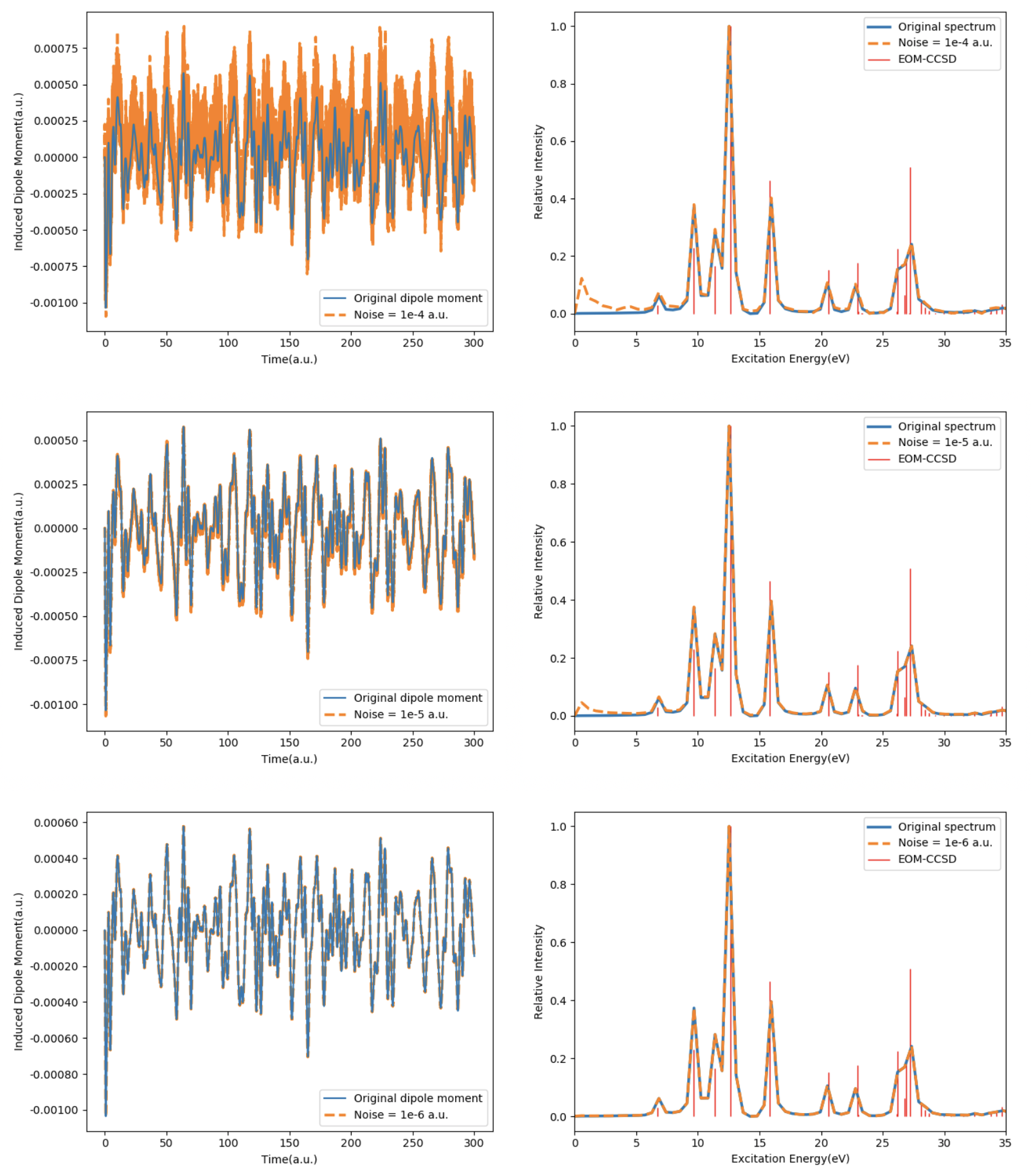
Figure 1: RT-CCSD/cc-pVDZ time-dependent induced electric dipole moments (left-hand column) for a water molecule in the presence of an external electric field and the corresponding linear absorption spectrum (right-hand column) with and without random noise of varying magnitudes. Corresponding EOM-CCSD/cc-pVDZ transitions are included as stick-spectra for comparison.

To compare the double-precision and single-precision arithmetic directly, we calculated RT-CCSD/cc-pVDZ dipole trajectories and the corresponding linear absorption spectra using both representations for the series of (H₂O)_n clusters with $n=1-4$. For these simulations, the explicit integration was carried out using the Runge-Kutta 4th order integrator (RK4) with a step size $h=0.01$ a.u. The external field was chosen to be a Gaussian envelope defined in Eq. (17) with ${\cal E}=0.01$ a.u., $\nu=0.05$ a.u., and $\sigma=0.01$ a.u. (a narrow pulse). The results are aligned with the numerical experiments above, with no discernible difference in the spectra after lowering the arithmetic precision to single-precision. All the spectra are also compared with EOM-CCSD/cc-pVDZ calculations: we include 40 EOM-CC roots in each of the spectra, all of which are well-aligned with the associated RT-CC peaks. From this perspective, the computation time and the required size of memory can both be reduced by ca. a factor of two for the calculation of the spectra, as previously observed for electronic energies and other components of quantum chemical calculations.^{48, 49, 53, 70, 54} We note, however, that single-precision arithmetic may not be practical for certain numerically sensitive calculations, e.g., using higher-order numerical differentiation to extract linear and nonlinear response functions as reported by Ding et al.⁷¹ (In addition, we note that these spectra are not intended to reproduce vapor-phase experimental measurements, only to test the validity of the single-precision arithmetic approximation. Thus, any transitions appearing above the physical ionization limit are not physically realistic and are merely an artifact of the use of a finite basis set without representation of continuum states.)

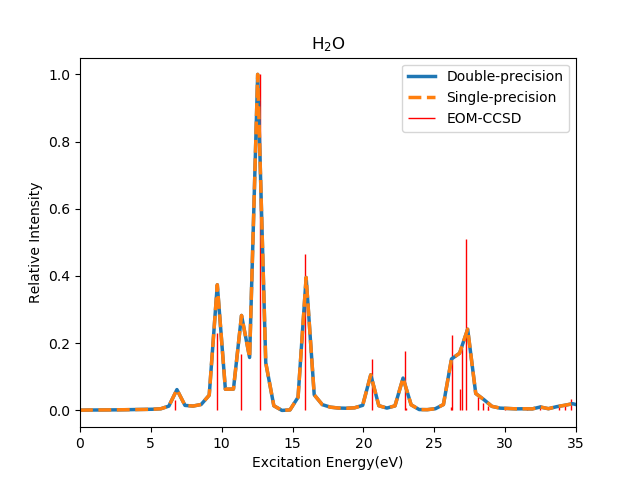
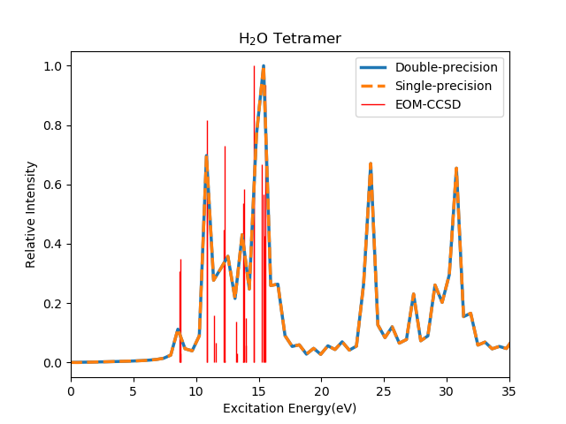
Figure 2: Linear UV/vis absorption spectra of (H₂O)_n clusters for $n=1-4$ calculated at the RT-CCSD/cc-pVDZ level of theory in both double- and single-precision arithmetic. Time propagation was carried out for 300 a.u. in the presence of a weak electric field represented by a narrow Gaussian pulse. Corresponding EOM-CCSD/cc-pVDZ transitions are included as stick-spectra for comparison.

Inspired by many parallel implementations of CC methods for distributed memory architectures on CPUs^{72, 73, 74, 75}, corresponding GPU implementations have become desirable in order to take advantage of heterogenous artchitectures on modern high-performance computing systems. While early GPU hardware was designed for accelerating image processing with an emphasis on mostly single- or low-precision floating point operations for quick memory access when higher accuracy is not required, over the past several years, GPUs have been more extensively used for scientific research. In addition to the development of GPUs with robust performance for double-precision arithmetic, numerous software toolkits have also emerged such as the Computer Unified Device Architecture (CUDA)⁷⁶, the Open Computing Language (OpenCL),⁷⁷ and a variety machine-learning packages that support GPUs such as TensorFlow,⁷⁸ PyTorch,⁶⁷ and others, all of which lower the barriers to a wide range of scientific applications that can take advantage of modern GPU performance. We note that, even though the performance of double-precision calculations on GPUs is already relatively robust, single-precision arithmetic is still preferable if it provides neglible errors relative to double-precision results due to the substantial improvement in computational speed and memory usage.

For the RT-CC methods explored in this work, we have therefore developed a GPU-capable implementation within the PyCC code using the PyTorch package⁶⁷ based on the conventional CPU version described in section 3. In the PyCC implementation, all one-electron quantities such as the Fock matrix (including the external field), $\hat{T}_{1}$, and $\hat{T}_{2}$ amplitudes are loaded onto the GPU at the beginning of either each iteration of the time-independent wave function or each computation of the residuals in Eqs. (5) and (6) during the RT-CC propagation. As each term in the CC equations is evaluated, the necessary subblock of the two-electron repulsion integrals is loaded onto the GPU, and the required tensor contraction is carried out using the usual opt_einsum function. Other two- and four-index intermediates formed from the similarity-transformed Hamiltonian (e.g., the $W_{mbej}$ or $W_{amef}$ intermediates), are retained on the GPU as they are created for later use in the same iteration/time-step, and deleted once the current residual is complete. The advantage of this approach is that it provides straightforward access to local GPU hardware without significant modification of the NumPy-based tensor-contraction code already in place. Of course, this Python-based implementation does not represent the full performance of a production-level code and is necessarily limited in terms of the size of the molecular system it can treat, but it does provide a valuable estimate of the minimum expected speed-up one can obtain for a more highly optimized alogrithm.

Table 2 provides a comparison of RT-CCSD/cc-pVDZ timings for double-precision (dp) and single-precision (sp) on CPUs and GPUs for our set of example water clusters, using the same Gaussian envelope parameters are for previous computations. The first three columns report the number of seconds required for each time step of the RT-CC simulation averaged over a 300 a.u. propagation (i.e., for a step size of $h=0.01$ a.u., averaged over 30,000 time steps). As the size of the molecular system increases from monomer to tetramer, the computational cost per iteration for a CPU-dp calculation increases by approximately a factor of ca. $4^{4.85}$, whereas for a GPU-dp calculation, the increase is a factor of ca. $4^{3.18}$, and for a GPU-sp calculation, this falls to $4^{2.88}$. While these are clearly less than the formal ${\cal O}(4^{6})$ scaling expected from CCSD, all of these implementations would eventually reach that limit for larger systems, because the CPU/GPU and dp/sp improvements only affect the prefactor, and not the exponent. Nevertheless, the use of the GPU coupled with single-precision arithmetic clearly offers substantial advantages. This improvement is also clearly seen in the data reported in the final two columns of Table 2, where the single-precision code yields roughly the expected factor of two speed-up over its double-precision counterpart (with both calculations taking place on the GPU), and the GPU offers up to a factor of 14 speed-up over the CPU when both operate in double-precision (or better when the GPU operates in single-precision mode). Larger molecular systems should offer even greater improvement, with the proviso that the memory limits of the GPU will eventually produce a performance pleateu.

Water Cluster	$t_{\textrm{CPU-dp}}$	$t_{\textrm{GPU-dp}}$	$t_{\textrm{GPU-sp}}$	$\frac{t_{\textrm{CPU-dp}}}{t_{\textrm{GPU-dp}}}$	$\frac{t_{\textrm{GPU-dp}}}{t_{\textrm{GPU-sp}}}$
Monomer	0.17217	0.14330	0.13253	1.2015	1.0813
Dimer	3.4705	0.60738	0.40496	5.7139	1.4999
Trimer	32.729	3.4910	1.7264	9.3752	2.0221
Tetramer	167.43	11.727	7.2215	14.277	1.6239

Table 2: Performance comparison of conventional RT-CC/cc-pVDZ calculations for water clusters using double-precision on the CPU (CPU-dp), double-precision on the GPU (GPU-dp), and single-precision on the GPU (GPU-dp). Timings (first three columns) are given in seconds as per-iteration averages over a 300 a.u. propagation wth $h=0.01$ a.u. The final two columns are speed-ups, i.e. ratios of timings for each case.

4.2 Comparison of Numerical Integrators for RT-CC

As discussed in section 2, the family of Runge-Kutta methods is the most widely used class of numerical integrators for IVPs such as the TDSE, not only because their implementation is straightforward — e.g., for RT-CC methods they are easily adapted to accept function vectors taken from the left- and right-hand wave function residuals in Eqs. (5) and (6) — but also because of their relatively robust performance for a range of applications. The classic Runge-Kutta 4th order integrator (RK4), for example, is one of the most commonly used algorithms for scientific problems because it averages each time step into four simple stages and yields a small truncation error of order $h^{5}$, where $h$ is the step size,

$$y_{n+1}=y_{n}+\frac{1}{6}(k_{1}+2k_{2}+2k_{3}+k_{4})+\textit{O}(h^{5}).$$ (19)

Such explicit integrators typically yield stable propagations of real-time methods, provided sufficient care is taken in choosing the step size, which is critical not only for the integration to be numerically stable, accurate, and efficient, but also cost effective: larger step sizes reduce the computational expense of the simulation, but they can also result in failure of the propagation due to a non-convergent time series. Rather than running sets of numerical experiments to find the largest, reasonable step size that can provide accurate results for every application, adaptive integrators⁵⁷ were designed to balance the required stability with the least computational cost by exerting algorithmic control over step size within the existing process of explicit integrators. For example, Fehlberg⁷⁹ discovered that, by carrying out six function evaluations per time step and using different combinations of the six resulting intermediates to formulate a fifth-order solution and a fourth-order solution, a fourth-order method can be derived with step size control. In 1990, Cash and Karp⁸⁰ found another combination of Fehlberg’s coefficients that yields an even more efficient method,

$$k_{1} =f(t_{n},y_{n})$$ (20)

$$k_{2} =f\left(t_{n}+\frac{1}{5}h,y_{n}+\frac{1}{5}k_{1}h\right)$$

$$k_{3} =f\left(t_{n}+\frac{3}{10}h,y_{n}+h\left(\frac{3}{40}k_{1}+\frac{9}{40}k_{2}\right)\right)$$

$$k_{4} =f\left(t_{n}+h,y_{n}+h\left(\frac{3}{10}k_{1}+\frac{9}{10}k_{2}+\frac{6}{5}k_{3}\right)\right)$$

$$k_{5} =f\left(t_{n}+\frac{3}{5}h,y_{n}+h\left(\frac{-11}{54}k_{1}+\frac{5}{2}k_{2}-\frac{70}{27}k_{3}+\frac{35}{27}k_{4}\right)\right)$$

$$k_{6} =f\left(t_{n}+\frac{7}{8}h,y_{n}+h\left(\frac{1631}{55296}k_{1}+\frac{175}{512}k_{2}-\frac{575}{13824}k_{3}+\frac{44275}{110592}k_{4}+\frac{253}{4096}k_{5}\right)\right),$$

with the resulting coupled time steps being,

$$y_{1} =y_{n}+h\left(\frac{37}{378}k_{1}+\frac{250}{621}k_{3}+\frac{125}{594}k_{4}+\frac{512}{1771}k_{6}\right)$$ (21)

$$y_{2} =y_{n}+h\left(\frac{2825}{27648}k_{1}+\frac{18575}{48384}k_{3}+\frac{13525}{55296}k_{4}+\frac{277}{14336}k_{5}+\frac{1}{4}k_{6}\right)$$

where $y_{1}$ is a fourth-order solution embedded with $y_{2}$, which is a fifth-order solution. Therefore, with $\Delta=|y_{2}-y_{1}|$ taken to be an error estimate for the current time step of order $h^{5}$, a desired accuracy of $\epsilon$ yields a formula for adjusting the step-size on the fly, viz.,

$$\frac{h_{new}}{h}=\left(\frac{\epsilon}{\Delta}\right)^{1/5}.$$ (22)

Thus, if $\Delta$ is smaller than $\epsilon$, $h$ will be increased for the next step, but if $\Delta$ is larger than $\epsilon$, $h$ will be reduced and the current step must be repeated until the required accuracy is reached. Furthermore, if $h$ is reduced and used for the current step again, the error will have an implicit scaling of $h$, and the exponent in Eq. (22) must be shifted from $\frac{1}{5}$ to $\frac{1}{4}$. The size control of final step is given as,

$$h_{new} =0.84h\left(\frac{\epsilon}{\Delta}\right)^{1/5}\hskip 14.22636pt \textrm{for}\hskip 2.84544pt|\Delta|\leq\epsilon$$ (23)

$$h_{new} =0.84h\left(\frac{\epsilon}{\Delta}\right)^{1/4}\hskip 14.22636pt \textrm{for}\hskip 2.84544pt|\Delta|>\epsilon$$

where the coefficient $0.84$ is a “safety factor” because the error estimates are not exact. Thus, the computational cost of the adaptive integrator is optimized under a predetermined desired accuracy. If the values at consecutive time steps change rapidly, a small step size will naturally be used; if the values vary only slightly, larger step sizes will be sufficient for a stable propagation.

In our RT-CC calculations, the time-dependent cluster amplitudes change rapidly when the external field is on at the beginning of the simulation and gradually stabilize after the field is turned off. With this in mind, we tested the adaptive Cash-Karp (CK) integrator described above for the RT-CCSD simulation of the absorption spectrum of a single water molecule using the same external field as in the calculations in section 4.1. Additionally, with the results shown in section 4.1, all the calculations are run in single-precision for the efficiency.

Fig. 3 reports the variation in the step size at each iteration of the propagation using an initial step size of $h=0.01$ a.u. From Eq. (17), if $t=0.01$ a.u. the field strength is only $3.35\times 10^{-6}$ a.u., and the local error $\Delta$, is expected to be smaller than $\epsilon$ according to Eq. (23), leading to an increase in $h$ to 0.015 a.u. At the second time step when $t=0.025$ a.u., the corresponding field strength is $4.39\times 10^{-4}$ a.u., which gets closer to its peak of 0.01 a.u. At this point in the simulation, $\Delta$ is large, and the CK algorithm automatically reduces the step size to $h=0.012$ a.u. At the third and fourth time steps, $h$ slightly increases to 0.014 a.u., because, even though the field is still on, $h=0.012$ a.u. is small enough to keep $\Delta$ smaller than $\epsilon$. After the fifth time step, $h$ is increased to 0.018 a.u. and further 0.027 a.u. when $t=0.064~{}\textrm{to}~{}0.082$ a.u., because, during this point in the propagation, the field strength has already begun to decrease due to the brevity of the pulse. When the propagation reaches $t=0.109$ a.u., the magnitude of the field strength falls back to $10^{-10}$, $\Delta$ is small when $h=0.027$ a.u. is tested, and thus $h$ increases to 0.032 a.u. at the seventh time step and 0.057 a.u. at the eighth time step. Starting from the ninth time step when $t=0.198$ a.u., although the external field is essentially zero for the remainder of the propagation, the algorithm still converges to a step size of $h=0.02$ a.u. due to the continued oscillation of the amplitudes instigated by the pulse. Since the step size varies throughout the propagation, the dipole moments are not calculated at equally spaced time points, typical Fourier transform will not work, instead, we pre-process our data by interpolating the data points to an evenly spaced grid. Ultimately, after a 300 a.u. propagation, the adaptive CK integrator yields an overall speedup of 1.32 relative to the explicit RK4 integrator, yet, as shown in Fig. 4, the final absorption spectra obtained from each algorithm exhibit no significant differences. Thus, adaptive integrators such as the CK algorithm can provide an automated approach to systematically optimizing the step size depending on the system.

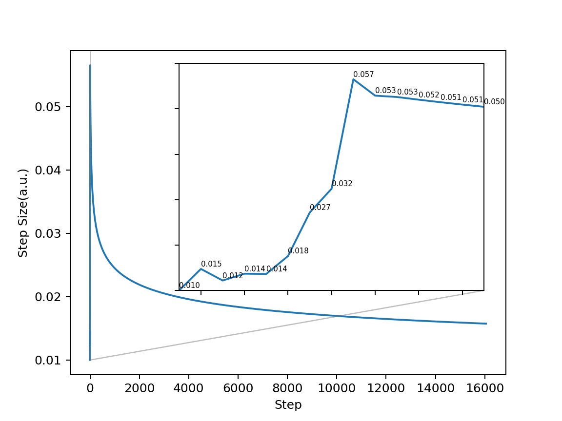
Figure 3: The adjusted step size at each time step in the RT-CCSD/cc-pVDZ calculation for H₂O using the adaptive Cash-Karp integrator over 300 a.u. propagation. The first 15 time steps are zoomed in to focus on the detailed change.

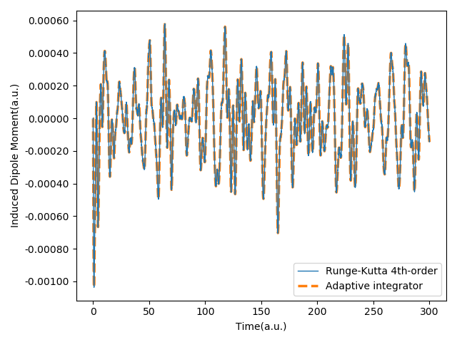
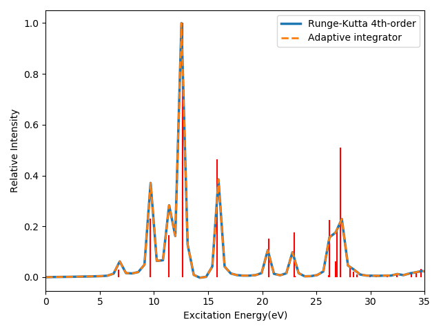
Figure 4: Comparison of the time-dependent induced dipole moment and the corresponding linear absorption spectrum from the RT-CCSD/cc-pVDZ simulation of H₂O using RK4 and CK integrators. EOM-CCSD/cc-pVDZ transition energies are depicted as stick-spectra for reference.

For strong external fields, the numerical stability of the propagation becomes challenging because the wave function amplitudes fluctuate rapidly leading to a large local error. For example, Fig. 5 depicts the norm of the $\hat{T}_{2}$ amplitudes from an RT-CCSD/cc-pVDZ simulation of our H₂O molecule at several different field strengths of the Gaussian pulse in Eq. (17) across a 1000 a.u. propagation using the RK4 integrator and a step size of $h=10^{-2}$ a.u. On the scale of the figure, the weaker fields of ${\cal E}=0.01$ and $1.0$ a.u. induce relatively small fluctuations in the amplitudes, while a $10.0$ a.u. field yields much larger oscillations. When the field strength is increased to ${\cal E}=100.0$ a.u.  the fluctuations are so great that the propagation diverges. In such cases, the TDSE is commonly referred to as a “stiff equation” in that the chosen step size must be extremely small to maintain the stability of the propagation. For our ${\cal E}=100.0$ a.u. test case, we find that a step size of $h=10^{-5}$ a.u. is necessary to maintain the integrity of the simulation, which is clearly impractical for realistic applications.

Figure 5: Comparison of the norm of $\hat{T}_{2}$ amplitudes during an RT-CC/cc-pVDZ simulation for H₂O using a short Gaussian pulse and the RK4 integrator for different field strengths, ${\cal E}$.

For the strong-field simulation, it is noteworthy that the divergence begins near the peak of the of the Gaussian pulse, suggesting that one might need only decrease the step size while the field is on (the “bumpy” portion of the trajectory) and shift to larger values once the field has decayed. We therefore carried out a test simulation using $h_{1}=10^{-5}$ a.u. when the field is non-zero and $h_{2}=0.01$ a.u. otherwise. The overhead of this approach is obviously the number of additional residual evaluations necessary during the pulse, $\frac{\Delta t}{h_{1}}-\frac{\Delta t}{h_{2}}$, where $\Delta t$ is the duration of the field. The goal is to use steps from $t_{0}$ to $t_{f}$ to track the interaction with the field precisely, while still minimizing the computational cost for the overall propagation.

In order to test this approach, we chose a very narrow Gaussian pulse with $\nu=0.0005$ a.u. and $\sigma=0.0001$ a.u. according to the magnitude of $h_{1}$, once again for an RT-CCSD/cc-pVDZ calculation for a single H₂O molecule, but for a 1000 a.u. propagation. For ${\cal E}=100.0$ a.u. we found that the proposed mixed-step-size approach recovered a stable propagation, as shown in Fig. 6, whose upper-left-hand plot depicts the norm of the $\hat{T}_{2}$ wave function parameters as a function of time. The amplitude of the oscillation is clearly greater than that induced by weaker fields, which is expected, but it still does not diverge throughout the propagation. The corresponding absorption spectrum in the lower-right-hand plot of Fig. 6 is nearly the same as that produced by a weaker field in Fig. 4, apart from some additional noise in the low-frequency regime.

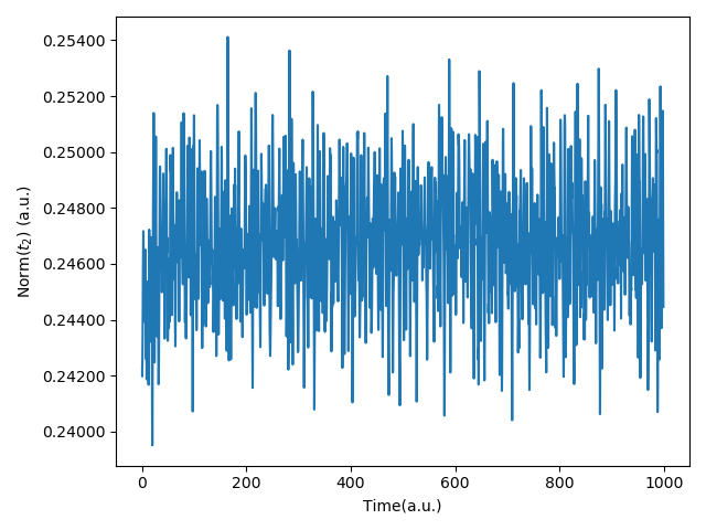
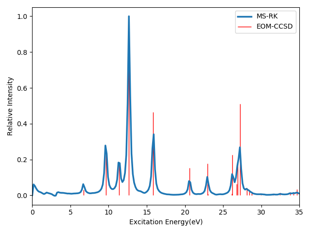
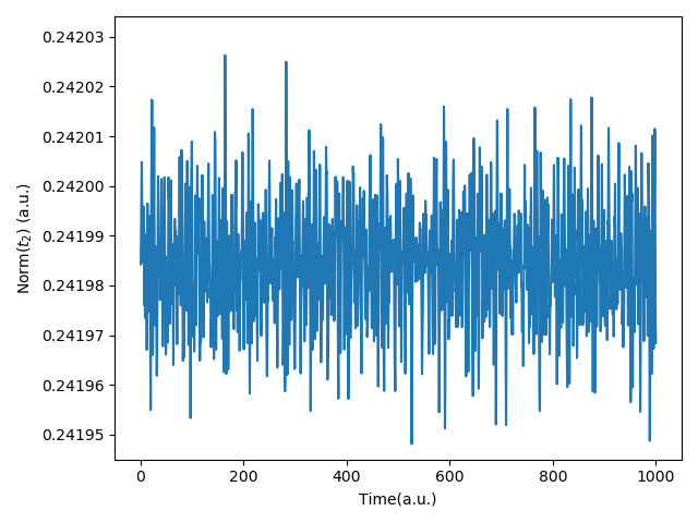
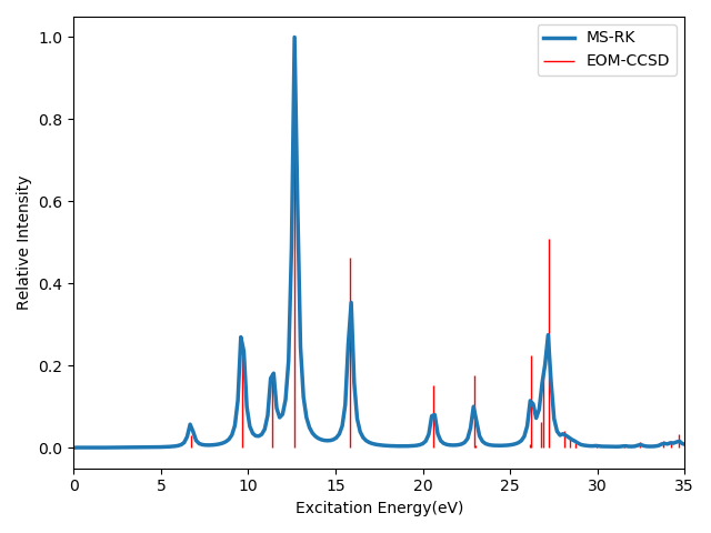
Figure 6: A $t=1000$ a.u. simulation of H₂O in the presence of a strong ${\cal E}=100.0$ a.u. field with a width of $10^{-4}$ a.u. (upper plots) and $10^{-6}$ a.u. (lower plots) at the RT-CCSD/cc-pVDZ level of theory using a mixed time-step RK4 approach. The norm of the $\hat{T}_{2}$ amplitudes are depicted in the left-hand plots, and the absorption spectrum is shown in the right-hand plots.

The low-frequency noise disappears, however, if we also choose an even narrower Gaussian pulse (so as to approximate a strong-field Dirac-delta pulse) in conjunction with the mixed step-size approach described above. To demonstrate this we chose parameters for the external field to be $\cal{E}=100$ a.u., $\sigma=10^{-6}$ a.u. and $\nu=5\times 10^{-6}$ a.u. with a corresponding step size of $h_{1}=10^{-7}$ a.u. during the pulse and the usual $h_{2}=0.01$ a.u. is used after field is off. (Note that we carried out this calculation in single-precision, and thus $10^{-7}$ is the smallest scale that can be selected to retain the required accuracy.) As shown in the lower plots of Fig. 6, the even smaller step size (compared to $h=10^{-5}$ a.u.) gives rise to a more stable propagation, and therefore, a higher-quality spectrum that avoids the extra noise in the low-frequency range that appears in the upper-right panel of Fig. 6. It should also be noted that the overhead of this calculation is the same as the one with a wider Gaussian pulse since the ratio $\frac{\Delta t}{h_{1}}$ is unchanged. Furthermore, while a mixed step-size approach will necessarily incur more overhead for more comples field shapes, the stability offered by the algorithm may be worth the additional expense. Finally we note that, while further testing is necessary to determine the robustness of this approach across a range of molecular systems, the propagation is stable even for the same molecule and the aug-cc-pVDZ basis set and with the oxygen $1s$-core electrons included in the correlation treatment.

5 Conclusions

In this work, we have explored several approaches for improving the efficiency of the real-time coupled cluster singles and doubles method. Through a number of numerical experiments on absorption spectra of small clusters of water molecules, we have found that lowering the arithmetic representation of the wave function from double- to single-precision yields negligible differences in the resulting spectra, but speeds up the calculations by nearly a factor of two compared to the conventional double-precision implementation. We have additionally found that migration of the data and the corresponding tensor contractions from CPU to GPU utilizing the the PyTorch framework produces a further overall speedup of a factor of 14. Based on the rapidly growing computational power of GPU hardware and their supporting software ecosystem, we intend to carry out further investigation and optimization of our GPU implementation for calculations on larger molecular systems.

We have also investigated a variety of numerical integration schemes for improving the stability and efficiency of the RT-CC approach, especially focusing on adaptive integrators that can adjust the step size during the time-propagation. In particular, we demonstrate that the Cash-Karp integrator, which uses an estimate of the local error in each iteration, can accordingly adjust the time-step to optimize the simulation in terms of both computing time and numerical stability. However, for very strong external fields, such as a narrow Gaussian envelope or delta-pulse, both of which are commonly used in such simulations, we find that even a straightforward mixed-step integrator based on the fourth-order Runge-Kutta algorithm is capable of providing a stable propagation provided a small enough step size is used in for the duration of the field. Such an algorithm should be quite favorable for such calculations with intense, but narrow laser pulses since it enables the existing RT-CCSD method to be generally used without any substantial modification to the algorithm or excessively increased computational cost. While further tests are required to determine the generality and robustness of this approach, the current results are encouraging.

6 Acknowledgements

This research was supported by the U.S. National Science Foundation (grant CHE-1900420). The authors are grateful to Prof. Thomas B. Pedersen and Håkon Kristiansen of the University of Oslo for helpful discussions and to Advanced Research Computing at Virginia Tech for providing computational resources and technical support that have contributed to the results reported within the paper.

References

- McCullough Jr and Wyatt 1969 McCullough Jr, E. A.; Wyatt, R. E. Quantum dynamics of the collinear (H, H2) reaction. The Journal of Chemical Physics 1969, 51, 1253–1254
- Kosloff 1988 Kosloff, R. Time-dependent quantum-mechanical methods for molecular dynamics. The Journal of Physical Chemistry 1988, 92, 2087–2100
- Li et al. 2020 Li, X.; Govind, N.; Isborn, C.; DePrince III, A. E.; Lopata, K. Real-time time-dependent electronic structure theory. Chemical Reviews 2020, 120, 9951–9993
- Li et al. 2005 Li, X.; Smith, S. M.; Markevitch, A. N.; Romanov, D. A.; Levis, R. J.; Schlegel, H. B. A time-dependent Hartree–Fock approach for studying the electronic optical response of molecules in intense fields. Physical Chemistry Chemical Physics 2005, 7, 233–239
- Repisky et al. 2015 Repisky, M.; Konecny, L.; Kadek, M.; Komorovsky, S.; Malkin, O. L.; Malkin, V. G.; Ruud, K. Excitation energies from real-time propagation of the four-component Dirac–Kohn–Sham equation. Journal of chemical theory and computation 2015, 11, 980–991
- Goings et al. 2018 Goings, J. J.; Lestrange, P. J.; Li, X. Real-time time-dependent electronic structure theory. Wiley Interdisciplinary Reviews: Computational Molecular Science 2018, 8, e1341
- Klamroth 2003 Klamroth, T. Laser-driven electron transfer through metal-insulator-metal contacts: Time-dependent configuration interaction singles calculations for a jellium model. Physical Review B 2003, 68, 245421
- Schlegel et al. 2007 Schlegel, H. B.; Smith, S. M.; Li, X. Electronic optical response of molecules in intense fields: Comparison of TD-HF, TD-CIS, and TD-CIS (D) approaches. The Journal of Chemical Physics 2007, 126, 244110
- Huber and Klamroth 2011 Huber, C.; Klamroth, T. Explicitly time-dependent coupled cluster singles doubles calculations of laser-driven many-electron dynamics. The Journal of Chemical Physics 2011, 134, 054113
- Nascimento and DePrince III 2017 Nascimento, D. R.; DePrince III, A. E. Simulation of near-edge X-ray absorption fine structure with time-dependent equation-of-motion coupled-cluster theory. The Journal of Physical Chemistry Letters 2017, 8, 2951–2957
- Kristiansen et al. 2020 Kristiansen, H. E.; Schøyen, Ø. S.; Kvaal, S.; Pedersen, T. B. Numerical stability of time-dependent coupled-cluster methods for many-electron dynamics in intense laser pulses. The Journal of Chemical Physics 2020, 152, 071102
- Sánchez-de Armas et al. 2010 Sánchez-de Armas, R.; Oviedo Lopez, J.; A. San-Miguel, M.; Sanz, J. F.; Ordejón, P.; Pruneda, M. Real-time TD-DFT simulations in dye sensitized solar cells: the electronic absorption spectrum of alizarin supported on TiO2 nanoclusters. Journal of Chemical Theory and Computation 2010, 6, 2856–2865
- Kolesov et al. 2016 Kolesov, G.; Grånäs, O.; Hoyt, R.; Vinichenko, D.; Kaxiras, E. Real-time TD-DFT with classical ion dynamics: Methodology and applications. Journal of Chemical Theory and Computation 2016, 12, 466–476
- Provorse and Isborn 2016 Provorse, M. R.; Isborn, C. M. Electron dynamics with real-time time-dependent density functional theory. International Journal of Quantum Chemistry 2016, 116, 739–749
- Bruner et al. 2016 Bruner, A.; LaMaster, D.; Lopata, K. Accelerated broadband spectra using transition dipole decomposition and Padé approximants. Journal of Chemical Theory and Computation 2016, 12, 3741–3750
- Goings and Li 2016 Goings, J. J.; Li, X. An atomic orbital based real-time time-dependent density functional theory for computing electronic circular dichroism band spectra. The Journal of Chemical Physics 2016, 144, 234102
- Bartlett 2010 Bartlett, R. J. The coupled-cluster revolution. Molecular Physics 2010, 108, 2905–2920
- Crawford and Schaefer 2000 Crawford, T. D.; Schaefer, H. F. An introduction to coupled cluster theory for computational chemists. Reviews in computational chemistry 2000, 14, 33–136
- Pedersen and Kvaal 2019 Pedersen, T. B.; Kvaal, S. Symplectic integration and physical interpretation of time-dependent coupled-cluster theory. The Journal of chemical physics 2019, 150, 144106
- Pedersen et al. 2020 Pedersen, T. B.; Kristiansen, H. E.; Bodenstein, T.; Kvaal, S.; Schøyen, Ø. S. Interpretation of Coupled-Cluster Many-Electron Dynamics in Terms of Stationary States. Journal of Chemical Theory and Computation 2020, 17, 388–404
- Nascimento and DePrince III 2016 Nascimento, D. R.; DePrince III, A. E. Linear absorption spectra from explicitly time-dependent equation-of-motion coupled-cluster theory. Journal of Chemical Theory and Computation 2016, 12, 5834–5840
- Nascimento and DePrince III 2019 Nascimento, D. R.; DePrince III, A. E. A general time-domain formulation of equation-of-motion coupled-cluster theory for linear spectroscopy. The Journal of Chemical Physics 2019, 151, 204107
- Koulias et al. 2019 Koulias, L. N.; Williams-Young, D. B.; Nascimento, D. R.; DePrince III, A. E.; Li, X. Relativistic real-time time-dependent equation-of-motion coupled-cluster. Journal of Chemical Theory and Computation 2019, 15, 6617–6624
- Vila et al. 2020 Vila, F. D.; Rehr, J. J.; Kas, J. J.; Kowalski, K.; Peng, B. Real-time coupled-cluster approach for the cumulant Green’s function. Journal of Chemical Theory and Computation 2020, 16, 6983–6992
- Park et al. 2019 Park, Y. C.; Perera, A.; Bartlett, R. J. Equation of motion coupled-cluster for core excitation spectra: Two complementary approaches. The Journal of Chemical Physics 2019, 151, 164117
- Park et al. 2021 Park, Y. C.; Perera, A.; Bartlett, R. J. Equation of motion coupled-cluster study of core excitation spectra II: Beyond the dipole approximation. The Journal of Chemical Physics 2021, 155, 094103
- Cooper et al. 2021 Cooper, B. C.; Koulias, L. N.; Nascimento, D. R.; Li, X.; DePrince III, A. E. Short Iterative Lanczos Integration in Time-Dependent Equation-of-Motion Coupled-Cluster Theory. The Journal of Physical Chemistry A 2021, 125, 5438–5447
- Pulay 1983 Pulay, P. Localizability of dynamic electron correlation. Chemical Physics Letters 1983, 100, 151–154
- Hampel and Werner 1996 Hampel, C.; Werner, H.-J. Local treatment of electron correlation in coupled cluster theory. The Journal of Chemical Physics 1996, 104, 6286–6297
- Neese et al. 2009 Neese, F.; Hansen, A.; Liakos, D. G. Efficient and accurate approximations to the local coupled cluster singles doubles method using a truncated pair natural orbital basis. The Journal of chemical physics 2009, 131, 064103
- Schütz and Werner 2001 Schütz, M.; Werner, H.-J. Low-order scaling local electron correlation methods. IV. Linear scaling local coupled-cluster (LCCSD). The Journal of Chemical Physics 2001, 114, 661–681
- Yang et al. 2012 Yang, J.; Chan, G. K.-L.; Manby, F. R.; Schütz, M.; Werner, H.-J. The orbital-specific-virtual local coupled cluster singles and doubles method. The Journal of Chemical Physics 2012, 136, 144105
- Russ and Crawford 2004 Russ, N. J.; Crawford, T. D. Local correlation in coupled cluster calculations of molecular response properties. Chemical physics letters 2004, 400, 104–111
- McAlexander et al. 2012 McAlexander, H. R.; Mach, T. J.; Crawford, T. D. Localized optimized orbitals, coupled cluster theory, and chiroptical response properties. Physical Chemistry Chemical Physics 2012, 14, 7830–7836
- Crawford et al. 2019 Crawford, T. D.; Kumar, A.; Bazanté, A. P.; Di Remigio, R. Reduced-scaling coupled cluster response theory: Challenges and opportunities. Wiley Interdisciplinary Reviews: Computational Molecular Science 2019, 9, e1406
- Gordon et al. 2012 Gordon, M. S.; Fedorov, D. G.; Pruitt, S. R.; Slipchenko, L. V. Fragmentation methods: A route to accurate calculations on large systems. Chemical reviews 2012, 112, 632–672
- Epifanovsky et al. 2013 Epifanovsky, E.; Zuev, D.; Feng, X.; Khistyaev, K.; Shao, Y.; Krylov, A. I. General implementation of the resolution-of-the-identity and Cholesky representations of electron repulsion integrals within coupled-cluster and equation-of-motion methods: Theory and benchmarks. The Journal of chemical physics 2013, 139, 134105
- Li and Li 2004 Li, W.; Li, S. Divide-and-conquer local correlation approach to the correlation energy of large molecules. The Journal of chemical physics 2004, 121, 6649–6657
- Li et al. 2009 Li, W.; Piecuch, P.; Gour, J. R.; Li, S. Local correlation calculations using standard and renormalized coupled-cluster approaches. The Journal of chemical physics 2009, 131, 114109
- Kinoshita et al. 2003 Kinoshita, T.; Hino, O.; Bartlett, R. J. Singular value decomposition approach for the approximate coupled-cluster method. The Journal of chemical physics 2003, 119, 7756–7762
- Koch et al. 2003 Koch, H.; Sánchez de Merás, A.; Pedersen, T. B. Reduced scaling in electronic structure calculations using Cholesky decompositions. The Journal of chemical physics 2003, 118, 9481–9484
- Hohenstein et al. 2012 Hohenstein, E. G.; Parrish, R. M.; Martínez, T. J. Tensor hypercontraction density fitting. I. Quartic scaling second-and third-order Møller-Plesset perturbation theory. The Journal of chemical physics 2012, 137, 044103
- Schutski et al. 2017 Schutski, R.; Zhao, J.; Henderson, T. M.; Scuseria, G. E. Tensor-structured coupled cluster theory. The Journal of chemical physics 2017, 147, 184113
- Parrish et al. 2019 Parrish, R. M.; Zhao, Y.; Hohenstein, E. G.; Martínez, T. J. Rank reduced coupled cluster theory. I. Ground state energies and wavefunctions. The Journal of chemical physics 2019, 150, 164118
- Pawłowski et al. 2019 Pawłowski, F.; Olsen, J.; Jørgensen, P. Cluster perturbation theory. I. Theoretical foundation for a coupled cluster target state and ground-state energies. The Journal of chemical physics 2019, 150, 134108
- Nascimento and DePrince III 2016 Nascimento, D. R.; DePrince III, A. E. Linear absorption spectra from explicitly time-dependent equation-of-motion coupled-cluster theory. Journal of chemical theory and computation 2016, 12, 5834–5840
- Yasuda 2008 Yasuda, K. Two-electron integral evaluation on the graphics processor unit. Journal of Computational Chemistry 2008, 29, 334–342
- Ufimtsev and Martinez 2008 Ufimtsev, I. S.; Martinez, T. J. Graphical processing units for quantum chemistry. Computing in Science & Engineering 2008, 10, 26–34
- Ufimtsev and Martinez 2008 Ufimtsev, I. S.; Martinez, T. J. Quantum chemistry on graphical processing units. 1. Strategies for two-electron integral evaluation. Journal of Chemical Theory and Computation 2008, 4, 222–231
- Luehr et al. 2011 Luehr, N.; Ufimtsev, I. S.; Martinez, T. J. Dynamic precision for electron repulsion integral evaluation on graphical processing units (GPUs). Journal of Chemical Theory and Computation 2011, 7, 949–954
- Vogt et al. 2008 Vogt, L.; Olivares-Amaya, R.; Kermes, S.; Shao, Y.; Amador-Bedolla, C.; Aspuru-Guzik, A. Accelerating resolution-of-the-identity second-order Møller- Plesset quantum chemistry calculations with graphical processing units. The Journal of Physical Chemistry A 2008, 112, 2049–2057
- DePrince III and Hammond 2011 DePrince III, A. E.; Hammond, J. R. Coupled cluster theory on graphics processing units I. The coupled cluster doubles method. Journal of chemical theory and computation 2011, 7, 1287–1295
- Asadchev and Gordon 2012 Asadchev, A.; Gordon, M. S. Mixed-precision evaluation of two-electron integrals by Rys quadrature. Computer Physics Communications 2012, 183, 1563–1567
- Pokhilko et al. 2018 Pokhilko, P.; Epifanovsky, E.; Krylov, A. I. Double precision is not needed for many-body calculations: Emergent conventional wisdom. Journal of Chemical Theory and Computation 2018, 14, 4088–4096
- Butcher 1996 Butcher, J. C. A history of Runge-Kutta methods. Applied numerical mathematics 1996, 20, 247–260
- Butcher 1963 Butcher, J. C. Coefficients for the study of Runge-Kutta integration processes. Journal of the Australian Mathematical Society 1963, 3, 185–201
- Press and Teukolsky 1992 Press, W. H.; Teukolsky, S. A. Adaptive Stepsize Runge-Kutta Integration. Computers in Physics 1992, 6, 188–191
- Bastani and Hosseini 2007 Bastani, A. F.; Hosseini, S. M. A new adaptive Runge–Kutta method for stochastic differential equations. Journal of computational and applied mathematics 2007, 206, 631–644
- Cameron and Gani 1988 Cameron, I.; Gani, R. Adaptive Runge-Kutta algorithms for dynamic simulation. Computers & chemical engineering 1988, 12, 705–717
- Stanton et al. 1991 Stanton, J. F.; Gauss, J.; Watts, J. D.; Bartlett, R. J. A direct product decomposition approach for symmetry exploitation in many-body methods. I. Energy calculations. The Journal of Chemical Physics 1991, 94, 4334–4345
- Buckingham 1967 Buckingham, A. D. Permanent and induced molecular moments and long-range intermolecular forces. Advances in Chemical Physics: Intermolecular Forces 1967, 107–142
- Barron 2009 Barron, L. D. Molecular light scattering and optical activity; Cambridge University Press, 2009
- 63 Crawford, T. D.; Peyton, B. G.; Wang, Z. http://github.com/CrawfordGroup/pycc
- Harris et al. 2020 Harris, C. R.; Millman, K. J.; Van Der Walt, S. J.; Gommers, R.; Virtanen, P.; Cournapeau, D.; Wieser, E.; Taylor, J.; Berg, S.; Smith, N. J., et al. Array programming with NumPy. Nature 2020, 585, 357–362
- Smith and Gray 2018 Smith, D. G. A.; Gray, J. Opt_einsum-a python package for optimizing contraction order for einsum-like expressions. Journal of Open Source Software 2018, 3, 753
- Smith et al. 2020 Smith, D. G.; Burns, L. A.; Simmonett, A. C.; Parrish, R. M.; Schieber, M. C.; Galvelis, R.; Kraus, P.; Kruse, H.; Di Remigio, R.; Alenaizan, A., et al. PSI4 1.4: Open-source software for high-throughput quantum chemistry. The Journal of chemical physics 2020, 152, 184108
- Paszke et al. 2019 Paszke, A.; Gross, S.; Massa, F.; Lerer, A.; Bradbury, J.; Chanan, G.; Killeen, T.; Lin, Z.; Gimelshein, N.; Antiga, L., et al. Pytorch: An imperative style, high-performance deep learning library. Advances in neural information processing systems 2019, 32
- Dunning Jr 1989 Dunning Jr, T. H. Gaussian basis sets for use in correlated molecular calculations. I. The atoms boron through neon and hydrogen. The Journal of chemical physics 1989, 90, 1007–1023
- Committee et al. 2019 Committee, M. S., et al. IEEE standard for floating-point arithmetic. IEEE Std 754-2019 (Revision of IEEE 754-2008). IEEE Computer Society, New York, NY, USA 2019,
- Tornai et al. 2019 Tornai, G. J.; Ladjánszki, I.; Rák, Á.; Kis, G.; Cserey, G. Calculation of quantum chemical two-electron integrals by applying compiler technology on GPU. Journal of Chemical Theory and Computation 2019, 15, 5319–5331
- Ding et al. 2013 Ding, F.; Van Kuiken, B. E.; Eichinger, B. E.; Li, X. An efficient method for calculating dynamical hyperpolarizabilities using real-time time-dependent density functional theory. The Journal of Chemical Physics 2013, 138, 064104
- Olson et al. 2007 Olson, R. M.; Bentz, J. L.; Kendall, R. A.; Schmidt, M. W.; Gordon, M. S. A novel approach to parallel coupled cluster calculations: Combining distributed and shared memory techniques for modern cluster based systems. Journal of Chemical Theory and Computation 2007, 3, 1312–1328
- Solomonik et al. 2014 Solomonik, E.; Matthews, D.; Hammond, J. R.; Stanton, J. F.; Demmel, J. A massively parallel tensor contraction framework for coupled-cluster computations. Journal of Parallel and Distributed Computing 2014, 74, 3176–3190
- Janowski et al. 2007 Janowski, T.; Ford, A. R.; Pulay, P. Parallel calculation of coupled cluster singles and doubles wave functions using array files. Journal of Chemical Theory and Computation 2007, 3, 1368–1377
- Anisimov et al. 2014 Anisimov, V. M.; Bauer, G. H.; Chadalavada, K.; Olson, R. M.; Glenski, J. W.; Kramer, W. T.; Apra, E.; Kowalski, K. Optimization of the coupled cluster implementation in NWChem on petascale parallel architectures. Journal of Chemical Theory and Computation 2014, 10, 4307–4316
- NVIDIA et al. 2020 NVIDIA,; Vingelmann, P.; Fitzek, F. H. CUDA, release: 10.2.89. 2020; \urlhttps://developer.nvidia.com/cuda-toolkit
- Stone et al. 2010 Stone, J. E.; Gohara, D.; Shi, G. OpenCL: A parallel programming standard for heterogeneous computing systems. Computing in science & engineering 2010, 12, 66
- Abadi et al. 2015 Abadi, M.; Agarwal, A.; Barham, P.; Brevdo, E.; Chen, Z.; Citro, C.; Corrado, G. S.; Davis, A.; Dean, J.; Devin, M.; Ghemawat, S.; Goodfellow, I.; Harp, A.; Irving, G.; Isard, M.; Jia, Y.; Jozefowicz, R.; Kaiser, L.; Kudlur, M.; Levenberg, J.; Mané, D.; Monga, R.; Moore, S.; Murray, D.; Olah, C.; Schuster, M.; Shlens, J.; Steiner, B.; Sutskever, I.; Talwar, K.; Tucker, P.; Vanhoucke, V.; Vasudevan, V.; Viégas, F.; Vinyals, O.; Warden, P.; Wattenberg, M.; Wicke, M.; Yu, Y.; Zheng, X. TensorFlow: Large-Scale Machine Learning on Heterogeneous Systems. 2015; \urlhttps://www.tensorflow.org/, Software available from tensorflow.org
- Fehlberg 1968 Fehlberg, E. Classical fifth-, sixth-, seventh-, and eighth-order Runge-Kutta formulas with stepsize control; National Aeronautics and Space Administration, 1968
- Cash and Karp 1990 Cash, J. R.; Karp, A. H. A variable order Runge-Kutta method for initial value problems with rapidly varying right-hand sides. ACM Transactions on Mathematical Software (TOMS) 1990, 16, 201–222