Frequency-domain digital predistortion
for Massive MU-MIMO-OFDM Downlink

Abstract

dpd is a method commonly used to compensate for the nonlinear effects of pa. However, the computational complexity of most dpd algorithms becomes an issue in the downlink of massive mu mimo ofdm, where potentially up to several hundreds of PAs in the bs require linearization. In this paper, we propose a cnn-based dpd in the frequency domain, taking place before the precoding, where the dimensionality of the signal space depends on the number of users, instead of the number of bs antennas. Simulation results on gmp-based pa show that the proposed cnn-based DPD can lead to very large complexity savings as the number of bs antenna increases at the expense of a small increase in power to achieve the same ser.

I Introduction

Massive mu-mimo is one of the prominent technologies in 5g and beyond. With proper precoding techniques, up to several hundreds of antennas at the bs increases the capacity when serving many tens of ue [1]. However, such large number of antennas poses a difficult linearization problem for the nonlinear pa. To meet the linearization performance of each pa, it is common to use dpd for each PA. However, the computational complexity increases linearly with the number of pa and becomes unacceptably large for massive MU-MIMO [2, 3].

To tackle this complexity problem, recent works have shifted toward reducing the number of dpd [2, 3, 4, 5], so that each dpd linearizes more than one single pa. These methods unavoidably degrade the linearization performance as each PA has a different behavior due to variations in component characteristics. Another research direction goes toward fd dpd [6, 7], where dpd is implemented before the ofdm idft. The complexity of the DPD is reduced as the DPD sampling rate becomes equal to the symbol rate, instead of using oversampling as in conventional dpd methods. While [6] considers hybrid massive MIMO, [7] considers a fully digital mu-mimo system with a nn-based DPD, where the dpd is implemented prior to the precoder. Thus, the complexity of the DPD is reduced as the dimensionality of the signal increases with the number of ue instead of the number of bs antennas. However, this method requires several idft and dft as the nn-based DPD still operates in the td. More problematically, the complexity cost of the method in [7] still increases with the number of bs antennas due to the additional precoding cost of the guard-band subcarriers. To address this complexity problem, an fd dpd model that only processes data subcarriers without idft would be a possible solution. To the best of our knowledge, such a model has not yet been proposed.

In this work, we consider a massive mu-mimo-ofdm system. We propose a cnn-based fd dpd model that takes place before the ofdm idft and the precoder. We refer to this model as FD-CNN. Compared with conventional td per-antenna dpd, the complexity cost of FD-CNN increases with the symbol rate and the number of ue instead of with the much higher sampling rate and the number of bs antennas. Furthermore, to avoid high complexity cost caused by the large number of data subcarriers at the DPD input, we consider 2d convolutional layers that can efficiently extract information from data subcarriers. We focus on the in-band metric ser as the out-of-band metric acpr requirements have been considerably relaxed in millimeter wave [8]. Simulation results on different gmp-based PA models at each antenna and a frequency-selective Rayleigh fading channel show that the proposed fd-CNN DPD can provide very large complexity savings when the number of bs antennas grows at the expense of a small increase in power to achieve the same ser performance compared with state-of-the-art TD and FD DPDs.

Notation: Lowercase and uppercase boldface letters denote column vectors and matrices such as $\boldsymbol{x}$ and $\boldsymbol{X}$; $\boldsymbol{x}^{\mathsf{H}}$ denotes the Hermitian transpose of $\boldsymbol{x}$; $\mathbb{R}$ and $\mathbb{C}$ denote real and complex numbers, respectively; $x_{n}$ or $[\boldsymbol{x}]_{n}$ denote the $n$-th element of $\boldsymbol{x}$, and $\boldsymbol{x}_{n:n+k}$ denotes a vector consisting of the $n$-th to $(n+k)$-th elements of $\boldsymbol{x}$; the $B\times U$ all-zeros matrix and the $U\times U$ identity matrix are denoted by $\boldsymbol{0}_{B\times U}$ and $\boldsymbol{I}_{U}$, respectively; $\mathbb{E}_{\boldsymbol{}}\{x\}$ denotes the expectation of $x$.

II System model

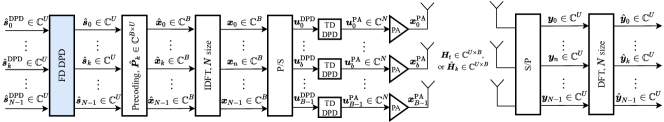
Figure 1: System model of a massive MU-MIMO-OFDM downlink with nonliner PAs in each RF chain of the BS. The conventional TD per-antenna DPDs take place before each PA while the proposed FD DPD operates before the precoder.

II-A System Model

We consider a massive MU-MIMO-OFDM downlink system model as shown in Fig. 1. The bs is equipped with $B$ antennas and transmits messages to $U\ll B$ single-antenna ue. Each OFDM symbol consists of $N$ subcarriers with $N_{\text{d}}$ data subcarriers and $N_{\text{g}}=N-N_{\text{d}}$ guard subcarriers. The subcarrier spacing is denoted by $\Delta f$. Accordingly, the sampling and symbol rate are defined as $f_{\text{s}}=N\Delta f$ and $f_{\text{d}}=N_{\text{d}}\Delta f$, respectively. The oversampling rate is $R=f_{\text{s}}/f_{\text{d}}=N/N_{\text{d}}$.

Specifically, let $\hat{\boldsymbol{s}}_{k}\in\mathbb{C}^{U}$ denote the symbol vector for $U$ ue at subcarrier $k$ in the fd, where all symbols are generated independently from an $M$-QAM constellation. A precoder maps $\hat{\boldsymbol{s}}_{k}$ to a $B$-dimensional antenna array based on the available csi. We consider linear precoders due to their low complexity and good performance [9]. Given the data vector $\hat{\boldsymbol{s}}_{k}$ at subcarrier $k$, the fd output of a linear precoder, $\hat{\boldsymbol{x}}_{k}\in\mathbb{C}^{B}$, is obtained by [10]

$$\hat{\boldsymbol{x}}_{k}=\hat{\boldsymbol{P}}_{k}\hat{\boldsymbol{s}}_{k}\,,$$ (1)

where $\hat{\boldsymbol{P}}_{k}\in\mathbb{C}^{B\times U}$ denotes the fd precoding matrix for subcarrier $k$. We consider the precoding matrices $\hat{\boldsymbol{P}}_{k}=\boldsymbol{0}_{B\times U}$ for guard subcarriers. The precoded vectors $\hat{\boldsymbol{x}}_{k}$ are transformed to td signals by $N$-size IDFTs. The td signal vector at time sample $n$, $\boldsymbol{x}_{n}\in\mathbb{C}^{B}$, is given by

$$\boldsymbol{x}_{n}=\frac{1}{\sqrt{N}}\sum_{k=0}^{N-1}\hat{\boldsymbol{x}}_{k}\exp\left(jk\frac{2\pi}{N}n\right)\,.$$ (2)

Without the impact of PA imperfections, the received signal at the $U$ UEs in the td at time sample $n$, $\boldsymbol{y}_{n}\in\mathbb{C}^{U}$, is given by [10]

$$\boldsymbol{y}_{n}=\sum_{t=0}^{T-1}\boldsymbol{H}_{t}\boldsymbol{x}_{n-t}+\boldsymbol{w}_{n}\,,$$ (3)

where $\boldsymbol{H}_{t}\in\mathbb{C}^{U\times B}$ denotes the td channel matrix at the $t$-th tap with a total of $T$ taps. The elements of the channel matrix are independently generated from a complex Gaussian distribution with zero mean and variance $T^{-1}$ [10]. The channel is assumed to be block-constant with a coherence time of one OFDM symbol. In addition, $\boldsymbol{w}_{n}\sim\mathcal{C}\mathcal{N}\left(\boldsymbol{0}_{U\times 1},N_{0}\boldsymbol{I}_{U}\right)$ denotes the awgn vector at time sample $n$ with the noise variance $N_{0}$. Note that this yields a spatially white frequency-selective Rayleigh-fading channel with uniform power-delay profile [10].

Equivalently, (3) can be written in the fd as

$$\hat{\boldsymbol{y}}_{k}=\hat{\boldsymbol{H}}_{k}\hat{\boldsymbol{x}}_{k}+\hat{\boldsymbol{w}}_{k},$$ (4)

where $\hat{\boldsymbol{H}}_{k}\in\mathbb{C}^{U\times B}=\sum_{t=0}^{T-1}\boldsymbol{H}_{t}\exp(-jk\frac{2\pi}{N}t)$ is the fd channel matrix at subcarrier $k$, $\hat{\boldsymbol{y}}_{k}\in\mathbb{C}^{U}=\sum_{n=0}^{N-1}\boldsymbol{y}_{n}\exp(-jk\frac{2\pi}{N}n)$ is the fd received signal at subcarrier $k$, and $\hat{\boldsymbol{w}}_{k}\in\mathbb{C}^{U}=\sum_{n=0}^{N-1}\boldsymbol{w}_{n}\exp(-jk\frac{2\pi}{N}n)$ is the fd AWGN noise at subcarrier $k$. Substituting (1) into (4), $\hat{\boldsymbol{y}}_{k}$ with precoder $\hat{\boldsymbol{P}}_{k}$ can be expressed as

$$\hat{\boldsymbol{y}}_{k}=\hat{\boldsymbol{H}}_{k}\hat{\boldsymbol{P}}_{k}\hat{\boldsymbol{s}}_{k}+\hat{\boldsymbol{w}}_{k}\,.$$ (5)

To minimize the MU interference, the pseudo-inverse of the channel matrix is used as the precoding matrix, which is known as the zf precoding. The precoding matrix $\hat{\boldsymbol{P}}_{k}$ in (5) can be expressed as [9]

$$\hat{\boldsymbol{P}}_{k}=\alpha\hat{\boldsymbol{H}}_{k}^{\mathsf{H}}(\hat{\boldsymbol{H}}_{k}\hat{\boldsymbol{H}}_{k}^{\mathsf{H}})^{-1},$$ (6)

where $\alpha$ denotes the normalization factor to ensure the power constraint $\mathbb{E}\left\{\|\hat{\boldsymbol{x}}_{k}\|^{2}\right\}=P_{T}$ is met. The expectation is over the symbols of all UEs, and $P_{T}$ denotes the average transmit power. With an imperfect knowledge of the csi, the BS has an estimated td channel matrix $\boldsymbol{H}_{t}^{\text{est}}=\sqrt{1-\eta}\boldsymbol{H}_{t}+\sqrt{\eta}\boldsymbol{H}_{t}^{\text{err}}$, where $\eta\in[0,1]$ and $\boldsymbol{H}_{t}^{\text{err}}\sim\mathcal{C}\mathcal{N}\left(\mathbf{0}_{U\times B},\boldsymbol{I}_{U\times B}\right)$ [10]. Thus, the fd channel matrix in (6) is replaced by a channel estimation $\hat{\boldsymbol{H}}_{k}^{\text{est}}=\sum_{t=0}^{T-1}\boldsymbol{H}_{t}^{\text{est}}\exp\left(-jk\frac{2\pi}{N}t\right)$.

II-B PA nonlinearity

After the IDFT, the td OFDM symbols are mapped to $B$ rf chains and sent to each td DPD with input at the $b$-th RF chain, $\boldsymbol{u}_{b}^{\text{DPD}}\in\mathbb{C}^{N}=[[\boldsymbol{x}_{0}]_{b},[\boldsymbol{x}_{1}]_{b},...,[\boldsymbol{x}_{N-1}]_{b}]^{\mathsf{T}}$. The DPD outputs are then converted to analog domain by the dac. For simplicity, we assume ideal dac with infinite-resolution. The PA input signal at the $b$-th RF chain is $\boldsymbol{u}_{b}^{\text{PA}}\in\mathbb{C}^{N}$. The PA associated with the $b$-th BS antenna is represented by the nonlinear function $f^{\mathrm{PA}}_{b}:\mathbb{C}^{L_{1}+1}\rightarrow\mathbb{C}$ with memory length $L_{1}$, input $[\boldsymbol{u}_{b}^{\text{PA}}]_{n:n-L_{1}}=\left[[\boldsymbol{u}_{b}^{\text{PA}}]_{n},\ldots,[\boldsymbol{u}_{b}^{\text{PA}}]_{n-L_{1}}\right]^{\mathsf{T}}\in\mathbb{C}^{L_{1}+1}$, and output $x^{\text{PA}}_{b,n}$. The input-output relation of the $b$-th PA at time sample $n$ can be expressed as

$$x^{\text{PA}}_{b,n}=f^{\mathrm{PA}}_{b}([\boldsymbol{u}_{b}^{\text{PA}}]_{n:n-L_{1}}).$$ (7)

Assuming an ideal PA with a linear behavior and with no need of DPD, (7) reduces to $x^{\text{PA}}_{b,n}=[\boldsymbol{u}_{b}^{\text{PA}}]_{n}=[\boldsymbol{u}_{b}^{\text{DPD}}]_{n}=[\boldsymbol{x}_{n}]_{b}$, where $[\boldsymbol{x}_{n}]_{b}$ is the $b$-th element of $\boldsymbol{x}_{n}$. With the PA gain, the average PA output power is defined as $P_{\text{PA}}=\mathbb{E}\{|x^{\text{PA}}_{b,n}|\}$, where the expectation is over all time steps and BS antennas. In this case, no ici is introduced, and MU interference is eliminated by the zf precoding, given perfect CSI. However, the PA nonlinearity creates distortion which in FD breaks the orthogonality of the subcarriers, and in spatial domain breaks the nulls created by the zf precoding. Thus, the nonlinear PAs cause both ici and MU interference.

II-C Time-domain DPD

DPD is applied to compensate for the nonlinear behavior of the PA. Conventionally, DPD is implemented in td before the PA and makes use of oversampling in order to cancel out adjacent channel power created by the PA nonlinearity. We represent the TD DPD associated with the $b$-th BS PA by a parametric model $f_{\boldsymbol{\theta}^{\text{DPD}}_{b}}:\mathbb{C}^{L_{2}+1}\rightarrow\mathbb{C}$ with parameters $\boldsymbol{\theta}_{b}^{\text{DPD}}$ and input memory length $L_{2}$. Then, the mapped analog td signal $\boldsymbol{u}_{b}^{\text{DPD}}$ is sent to the corresponding DPD as

$$u^{\text{PA}}_{b,n}=f_{\boldsymbol{\theta}^{\text{DPD}}_{b}}([\boldsymbol{u}_{b}^{\text{DPD}}]_{n:n-L_{2}}),$$ (8)

where the DPD output $u^{\text{PA}}_{b,n}$ corresponds to the PA input in (7). In the case of massive MU-MIMO, one can use one DPD for each PA. However, the total computational complexity cost of the DPD increases linearly with the number of PAs and antennas, which makes this approach highly impractical when several hundreds of PAs are deployed [2].

III Complexity Analysis of DPD Benchmarks in Massive MU-MIMO

III-A Measure of DPD Complexity

When working with DPD algorithm design, there are two complexity figures to consider, the running complexity and traning complexity. The running complexity is the computational complexity needed to continuously run the DPD algorithm, which makes it the major overall contributor to complexity. Unlike the training complexity, which is an offline cost, the running complexity directly relates to the number of operations required for the inference of a certain number of samples [11].

There are several ways to measure the running complexity of DPD such as the Bachmann-Landau measure $\mathcal{O}(\cdot)$, running time, and number of parameters. These measures are either approximations or depend on the specific type of platform and thus are implementation-dependent. In contrast, the number of flop can accurately measure every addition, subtraction, and multiplication operation for both Volterra series-based models [12] and NNs [13, 14] for DPD. We therefore utilize the number of flop to measure the running complexity of DPD, as this is the figure of merit which brings us closest to a fair comparison without going into implementation details. In this paper, we follow the same FLOP calculation as in [11, Table I]. In massive MU-MIMO, for a fair complexity comparison for different DPD schemes in the td and fd, we calculate the total number of FLOPs required per ue for one OFDM symbol.

III-B Time-domain Per-antenna GMP-based DPD

While there exist a large variety of published td DPD models, we choose the commonly used gmp [15] for comparison because it has been shown to outperform many other models in terms of linearization performance versus complexity [11]. For simplicity, we refer to this td per-antenna GMP method as TD-GMP.

To linearize every PA in massive MU-MIMO-OFDM, each RF chain deploys a GMP-based DPD with the same memory length $L_{3}$, nonlinear order $K$, and cross-term length $G$. Given the td signal, $\boldsymbol{u}_{b}$, at the $b$-th RF chain as the input, the output of the gmp-based DPD associated with the $b$-th RF chain at time sample $n$ can be expressed as

$$u^{\text{PA}}_{b,n}= \sum_{k=0}^{K-1}\sum_{l=0}^{L_{3}}a_{k,l}[\boldsymbol{u}_{b}^{\text{DPD}}]_{n-l}\big{|}[\boldsymbol{u}_{b}^{\text{DPD}}]_{n-l}\big{|}^{k}$$ (9)

$$+\sum_{k=1}^{K-1}\sum_{l=0}^{L_{3}}\sum_{g=1}^{G}\Big{(}b_{k,l,g}[\boldsymbol{u}_{b}^{\text{DPD}}]_{n-l}\big{|}[\boldsymbol{u}_{b}^{\text{DPD}}]_{n-l-g}\big{|}^{k}$$

$$+c_{k,l,g}[\boldsymbol{u}_{b}^{\text{DPD}}]_{n-l}\left|[\boldsymbol{u}_{b}^{\text{DPD}}]_{n-l+g}\right|^{k}\Big{)}\,,$$

where $a_{k,l}$, $b_{k,l,g}$, and $c_{k,m,g}$ are complex-valued coefficients, which are identified using conventional mse estimation.

The number of flop required for the GMP with each input sample is computed as [11]

$$C^{\text{TD-GMP}}_{\text{Samp}} =8\big{(}(L_{3}+1)(K+2KG)-\frac{G(G+1)}{2}(K-1)\big{)}$$

$$+10+2K+2(K-1)G+2K\min(G,L_{3})$$ (10)

Now consider that we use GMP-based DPD for each antenna in a massive MU-MIMO antenna system. The number of FLOPs required per ue for one OFDM symbol is calculated as

$$C^{\text{TD-GMP}}_{\text{}}=C^{\text{TD-GMP}}_{\text{Samp}}NB/U\,.$$ (11)

We note that the number of FLOPs for the td GMP-based DPD grows linearly with the number of bs antennas because every PA requires one DPD. This causes a complexity problem in massive MU-MIMO with hundreds of antennas.

Figure 2: Structure of the proposed FD-CNN. For the $u$-th UE, the input of FD-CNN is formed by a selection of $L_{\text{U}}$ UE symbol vectors, $\{\tilde{\boldsymbol{s}}_{u}^{\text{DPD}},\tilde{\boldsymbol{s}}_{\check{u}}^{\text{DPD}},...,\tilde{\boldsymbol{s}}_{\acute{u}}^{\text{DPD}}\}$. The output is the predistorted symbol vector of $u$-th UE, $\tilde{\boldsymbol{s}}_{u}$.

III-C fd Neural Network-based DPD

To address the complexity problem of td DPD in massive MU-MIMO, the authors in [7] proposed a nn-based DPD, which operates in the fd prior to the precoder. In this paper, we refer to this fd NN-based DPD model as FD-NN. To form the input of the FD-NN, each ue stream is first converted to the td. Specifically, given the symbol vector for the $u$-th ue in the fd, $\tilde{\boldsymbol{s}}_{u}^{\text{DPD}}\in\mathbb{C}^{N}=[[\hat{\boldsymbol{s}}_{0}^{\text{DPD}}]_{u},[\hat{\boldsymbol{s}}_{1}^{\text{DPD}}]_{u},...,[\hat{\boldsymbol{s}}_{N-1}^{\text{DPD}}]_{u}]^{\mathsf{T}}$, the td symbol vector for the $u$-th ue, $\boldsymbol{s}_{u}^{\text{DPD}}\in\mathbb{C}^{N}$, is given by an IDFT

$$\boldsymbol{s}_{u}^{\text{DPD}}=\frac{1}{\sqrt{N}}\sum_{k=0}^{N-1}[\tilde{\boldsymbol{s}}_{u}^{\text{DPD}}]_{k}\exp(jk\frac{2\pi}{N}n)=\boldsymbol{F}_{N}^{\mathsf{H}}\tilde{\boldsymbol{s}}_{u}^{\text{DPD}},$$ (12)

where $\boldsymbol{F}_{N}$ denotes the unitary $N\times N$ DFT matrix. Then, using tapped delay lines with memory length $L_{4}$, the input signal of the first layer consists of each td UE symbol vector, $[\boldsymbol{s}_{u}^{\text{DPD}}]_{n:n-L_{4}}=[[\boldsymbol{s}_{u}^{\text{DPD}}]_{n},[\boldsymbol{s}_{u}^{\text{DPD}}]_{n-1},...,[\boldsymbol{s}_{u}^{\text{DPD}}]_{n-L_{4}}]^{\mathsf{T}}\in\mathbb{C}^{L_{4}+1}$. In total, the input signal of the first layer FD-NN is given by

$$\boldsymbol{s}_{\text{In}}^{\text{FD-NN}}=[[\boldsymbol{s}_{0}^{\text{DPD}}]_{n:n-L_{4}}^{\mathsf{T}},[\boldsymbol{s}_{1}^{\text{DPD}}]_{n:n-L_{4}}^{\mathsf{T}},...,[\boldsymbol{s}_{U-1}^{\text{DPD}}]_{n:n-L_{4}}^{\mathsf{T}}]^{\mathsf{T}},$$ (13)

which is then decomposed into real and imaginary parts connecting with their own neurons. Thus, this yields $2U(L_{4}+1)$ neurons for the first layer. All layers in the FD-NN are fully connected. There are $K^{\text{NN}}$ hidden layers, each with $D$ neurons and a nonlinear activation function ReLU. The number of neurons at the output layer is $2U$. The predistorted td signal for each UE is then converted back to the fd by dft before being sent to the precoder.

In this method, the additional idft and dft introduce an extra complexity cost. More importantly, the guard subcarriers of the predistorted signal are not empty anymore due to the dft, which leads to extra complexity cost due to the precoding. For each UE, the number of flop required for the FD-NN per OFDM symbol can be computed as

$$C_{\text{}}^{\text{FD-NN}} =\frac{1}{U}\Big{(}\underbrace{N\big{(}4U(L_{3}+1)D+2(K^{\text{NN}}-1)D^{2}+4DU\big{)}}_{\text{NN}}$$

$$\quad+\underbrace{10UN\log_{2}N}_{\text{(I)DFTs}}+\underbrace{(6+2)N_{g}UB}_{\text{Extra precoding}}\Big{)},$$ (14)

where the $6$ and $2$ in the extra precoding part are for complex-number multiplication and addition, respectively. Considering the fast Fourier transform, the complexity of a $N$-size (I)DFT is approximated by $5N\log_{2}N$ FLOPs with $\frac{N}{2}\log_{2}N$ complex-number multiplications and $N\log_{2}N$ complex-number additions, and there are $U$ IDFTs and $U$ DFTs. We note that due to extra precoding cost, the number of FLOPs for FD-NN still increases with the number of BS antennas, which dominates the complexity when hundreds of antennas are deployed in massive MU-MIMO.

IV Proposed fd Convolutional Neural Network

IV-A Structure of the FD-CNN

The structure of the proposed FD-CNN is shown in Fig. 2. FD-CNN works in the fd with the input of UE symbol vectors. To efficiently extract appropriate information from the fd UE symbol vectors without using IDFTs as [6], we propose to use 2d convolutional layers as the first layer, which save complexity compared with a fully connected layer. To facilitate the 2D convolution, the fd UE symbol vector $\tilde{\boldsymbol{s}}_{u}^{\text{DPD}}\in\mathbb{C}^{N}$ is converted to a matrix $\tilde{\boldsymbol{S}}_{u}^{\text{DPD}}\in\mathbb{C}^{\lceil\sqrt{N_{\text{d}}}\rceil\times\lceil\sqrt{N_{\text{d}}}\rceil}$, where only $N_{\text{d}}$ data subcarriers are involved to save complexity. Here $\lceil\cdot\rceil$ denotes the ceiling function and zero-padding is used if $\lceil\sqrt{N_{\text{d}}}\rceil>\sqrt{N_{\text{d}}}$. To offer more complexity saving, for the $u$-th UE, an arbitrary selection of $L_{\text{U}}$ UE symbol vectors from all $U$ UEs, $\{\tilde{\boldsymbol{s}}_{u}^{\text{DPD}},\tilde{\boldsymbol{s}}_{\check{u}}^{\text{DPD}},...,\tilde{\boldsymbol{s}}_{\acute{u}}^{\text{DPD}}\}$, including $\tilde{\boldsymbol{s}}_{u}^{\text{DPD}}$, are converted to matrices. In total, these matrices form the input of the FD-CNN as a tensor, $\tilde{\mathcal{S}}_{u}\in\mathbb{C}^{\lceil\sqrt{N_{\text{d}}}\rceil\times\lceil\sqrt{N_{\text{d}}}\rceil\times L_{\text{U}}}$,

$$\tilde{\mathcal{S}}_{u}^{\text{DPD}}=[\tilde{\boldsymbol{S}}_{u}^{\text{DPD}},...,\tilde{\boldsymbol{S}}_{\check{u}}^{\text{DPD}},...,\tilde{\boldsymbol{S}}_{\acute{u}}^{\text{DPD}}].$$ (15)

Then, each complex-valued UE symbol matrix in $\tilde{\mathcal{S}}_{u}^{\text{DPD}}$ is decomposed into real and imaginary matrices with the same dimension as $\tilde{\boldsymbol{S}}_{u}^{\text{DPD}}$. In total, there are $2L_{\text{U}}$ real-valued UE symbol matrices, which are convoluted by $N^{\text{Conv}}$ convolutional kernels with the same kernel size $K_{\text{C}}$ and stride length $K_{\text{S}}$. This yields an output tensor, $\tilde{\mathcal{S}}_{u}^{\text{Conv}}\in\mathbb{R}^{\lceil\frac{\lceil\sqrt{N_{\text{d}}}\rceil}{K_{\text{S}}}\rceil\times\lceil\frac{\lceil\sqrt{N_{\text{d}}}\rceil}{K_{\text{S}}}\rceil\times N^{\text{Conv}}}$, where zero-padding is also considered if $\lceil\frac{\lceil\sqrt{N_{\text{d}}}\rceil}{K_{\text{S}}}\rceil>\frac{\lceil\sqrt{N_{\text{d}}}\rceil}{K_{\text{S}}}$.

$\tilde{\mathcal{S}}_{u}^{\text{Conv}}$ is passed through an element-wise activation function $\sigma(\cdot)$ and then flatten into a column vector, $\tilde{\boldsymbol{s}}_{u}^{\text{Flat}}\in\mathbb{R}^{\lceil\frac{\lceil\sqrt{N_{\text{d}}}\rceil}{K_{\text{S}}}\rceil\lceil\frac{\lceil\sqrt{N_{\text{d}}}\rceil}{K_{\text{S}}}\rceil N^{\text{Conv}}}$. After that $\tilde{\boldsymbol{s}}_{u}^{\text{Flat}}$ is fully connected with the linear output layer with $2N_{\text{d}}$ neurons, which correspond to the real and imaginary parts of the predistorted symbol vector at the $u$-th UE, $\tilde{\boldsymbol{s}}_{u}\in\mathbb{C}^{N_{\text{d}}}$.

IV-B Complexity Analysis

We split the complexity of the proposed FD-CNN into the convolution layer part and the fully-connected layer part. For the complexity of the convolution layer part, each $K_{\text{C}}$-size 2D convolution requires $(2K_{\text{C}}^{2}-1)$ flop consisting of $K_{\text{C}}^{2}$ real-valued multiplications and $(K_{\text{C}}^{2}-1)$ real-valued additions. This 2D convolution operates on $2L_{\text{U}}$ real-valued UE symbol matrices with stride length $K_{\text{S}}$, and in total there are $N^{\text{Conv}}$ convolutional kernels. Thus, the number of flop for the convolution layer part can be expressed as

$$C_{\text{Conv}}^{\text{FD-CNN}}=2N^{\text{Conv}}L_{\text{U}}(2K_{\text{C}}^{2}-1)\left(\frac{\lceil\sqrt{N_{\text{d}}}\rceil}{K_{\text{S}}}\right)^{2}.$$ (16)

The number of FLOPs for the fully-connected layer part can be expressed as

$$C_{\text{FC}}^{\text{FD-CNN}}=8N_{\text{d}}L_{\text{U}}\left(\frac{\lceil\sqrt{N_{\text{d}}}\rceil}{K_{\text{S}}}\right)^{2}.$$ (17)

In total, the number of flop required for the FD-CNN with one OFDM symbol per UE is calculated as

$$C^{\text{FD-CNN}} =C_{\text{Conv}}^{\text{FD-CNN}}+C_{\text{FC}}^{\text{FD-CNN}}$$ (18)

We note that $C^{\text{FD-CNN}}$ is sensitive to the number of data subcarriers $N_{\text{d}}$ because $C_{\text{FC}}^{\text{FD-CNN}}$ is in the magnitude of $N_{\text{d}}^{2}$. Compared with the complexity for TD-GMP and FD-NN in (11) and (14), we note that the complexity of FD-CNN does not depend on the number of BS antennas, $B$, which naturally saves complexity when $B$ is large in massive MU-MIMO.

V Numerical Results

V-A Simulation Setup

V-A1 Parameters

We consider a set of simulated PAs using the GMP model in (9) with nonlinear order $K=7$, memory length $M=3$, and cross-term length $G=1$. These parameters are estimated using real measurements from the RF WebLab using a $100$ MHz OFDM signal [16]. Using the estimated PA parameters as the mean of a Gaussian distribution, the PA parameters of each antenna are drawn with variance $0.01$. For instance, given the original GMP-based PA coefficient $\alpha_{k,l}$, the coefficient at $b$-th antenna $\alpha_{k,l}^{b}\sim\mathcal{N}(\alpha_{k,l},0.01\alpha_{k,l})$. Note the GMP-based PA coefficients are fixed once being generated. The saturation point and measurement noise standard deviation of each PA are $24.02$ V $(\approx 37.6$ dBm with a $50$ $\Omega$ load impedance) and $0.053$ V, respectively.

We select a $50$ MHz OFDM setup in the operating band n257 from the 3GPP 5G standardization [17, Table 5.3.2-1 and 5.3.5-1] with subcarrier spacing $\Delta f=120$ kHz, OFDM symbol length $N=4096$, number of data subcarriers $N_{\text{d}}=384$, and $M=256$ QAM modulation. Each channel realization has $T=10$ taps. The AWGN noise variance is $N_{0}=1$ Watts/Hz. We assume the BS has imperfect CSI with $\eta=0.001$, which affects the ZF precoding.

For the benchmark of TD-GMP, we consider the same GMP parameter setup for each DPD as the PA model, namely $K=7$, $L_{3}=3$, and $G=1$. For the benchmark of FD-NN, we consider the same memory length $L_{4}=3$. Other parameters are set the same as in [7] with $N_{\text{FD-NN}}=1$ hidden layer and $D=15$ neurons. For the proposed FD-CNN, we set $\left\lceil\sqrt{N_{\mathrm{d}}}\right\rceil=20$, $L_{\text{U}}=1$, $K_{\text{C}}=3$, and $K_{\text{S}}=1$, and $N^{\text{Conv}}=2$. The activation function $\sigma(\cdot)$ in the convolution layer is the ReLU. To preserve the same input and output dimension of the convolutional layer, zero padding is used.

V-A2 DPD Coefficients Identification

For the TD-GMP, the coefficients of each GMP-based DPD are estimated using the ila at the output of each PA [18], where the least squares algorithm is used to minimize the mse between the PA input signal and post-distorter output signal. For the FD-NN, since all blocks in the given communication system are simulated and differentiable, we simply utilize supervised learning with a loss function at the receiver side to minimize the mse between received symbols $\hat{\boldsymbol{y}}_{k}$ and transmitted symbols $\hat{\boldsymbol{s}}_{k}$ for all data subcarriers. This symbol-based criterion for DPD optimization has been shown to achieve similar SER performance in [19]. Note new channel realization is generated for every training mini-batch. The FD-NN is then trained till convergence using the gradient descent optimizer Adam [20] with a learning rate $0.001$.

For the proposed FD-CNN, we choose the same supervised learning, loss function, and optimizer Adam as the training for FD-NN. Each mini-batch consists of $10$ OFDM symbols. In practical applications, it is straightforward to use a training method similar to the one in [7]. This training method creates the training data of the NN output by converting back PA output signals through MP-based DPDs and the pseudo-inverse of precoders. This requires dedicated feedback paths to collect each PA output at the transmitter. Alternatively, one can use over-the-air method that utilize an observation receiver for data acquisition as in [21, 19].

V-B Simulation results

V-B1 Complexity Versus Number of BS Antennas

Figure 3: The number of FLOPs required for each DPD scheme with one UE and one OFDM symbol versus the number of BS antennas, $B$.

Fig. 3 shows the number of FLOPs for one OFDM symbol per UE as a function of the number of BS antennas, $B\in\{1,2,4,8,16,32,64,128,256,512,1024\}$, for DPD schemes of TD-GMP, FD-NN, and the proposed FD-CNN. We also plot results for different number of UEs, $U\in\{1,4,8\}$.

We note that, as $B$ increases, the number of FLOPs for TD-GMP grows linearly as each antenna is associated with one td DPD. While the number of FLOPs for FD-NN grows gently for $B<16$, it eventually increases linearly with $B$ as the extra cost of guard-band precoding starts to dominate. However, the number of FLOPs for the proposed FD-CNN is completely invariant to $B$, which would greatly benefit very large antenna systems. Compared with FD-NN and TD-GMP, FD-CNN saves around $2.2\times$ and $8.9\times$ FLOPs for $B=32$ and $U=8$, respectively, and these savings can be further increased up to $26\times$ and $286\times$ when $B$ increases to $1024$.

We also observe that as $U$ increases, the number of FLOPs per UE decreases accordingly for TD-GMP, while this number for FD-NN and FD-CNN is the same.

V-B2 SER Versus Average PA Output Power

Now we fix $B=32$ and $U=8$ for different DPD schemes from Fig. 3 and plot the ser results as a function of the average PA output power, $P_{\text{PA}}$, in Fig. 4. Specifically, we plot the case of ideal linear-clipping PA [22]. The linear-clipping PA has a linear behavior before the clipping region, which has the minimum distortion that any DPDs can achieve. The number of QAM symbols used to calculate the SER is around $10^{6}$.

We note that the SER curves exhibit two different behaviors depending on the nonlinear and clipping regions of the PAs. On one hand, as $P_{\text{PA}}$ is below $25$ dBm, most PAs in the massive MU-MIMO system operate in their linear/nonlinear regions, so the SER of all DPD cases improve dramatically with $P_{\text{PA}}$ since the snr at the UEs are increasing accordingly. The proposed FD-CNN requires $2.2\times$ and $8.9\times$ less complexity than TD-GMP and FD-NN, respectively, at the expense of some increase in the required power to achieve a certain SER. For example, it requires $0.8$ dBm and $1.8$ dBm more PA output power to achieve an SER $10^{-3}$. On the other hand, when $P_{\text{PA}}>25$ dBm, the clipping effect of the PA brings unrecoverable distortions, which lead to a quick SER degradation for all DPD cases. The SER gap between all the DPD cases and the linear-clipping case may come from some residual distortions due to irreversible nonlinearity.

Figure 4: SER as a function of the average PA output power, $P_{\text{PA}}$.

VI Conclusion

We proposed a novel DPD method in the FD based on CNNs to address the rising complexity issue of linearization for large antenna systems in massive MU-MIMO-OFDM. The complexity of the proposed FD-CNN DPD is in the magnitude of the number of UEs and the symbol rate, which naturally avoids high complexity as the number of BS antennas increases. Simulation results on a MU-MIMO-OFDM system with different behavior PAs on each RF chain show that the FD-CNN can save $2.2\times$ and $8.9\times$ number of FLOPs with $32$ BS antennas and $8$ UEs, compared with FD NN-based and TD per-antenna GMP-based DPDs, respectively. This saving can be further improved as the number of BS antennas increases. Furthermore, the SERs degradation of FD-CNN is minor.

References

- [1] E. G. Larsson, O. Edfors, F. Tufvesson, and T. L. Marzetta, “Massive MIMO for next generation wireless systems,” IEEE Commun. Mag., vol. 52, no. 2, pp. 186–195, Feb. 2014.
- [2] X. Liu, W. Chen, L. Chen, F. M. Ghannouchi, and Z. Feng, “Linearization for hybrid beamforming array utilizing embedded over-the-air diversity feedbacks,” IEEE Trans. Microw. Theory Techn., vol. 67, no. 12, pp. 5235–5248, Oct. 2019.
- [3] X. Wang, Y. Li, C. Yu, W. Hong, and A. Zhu, “Digital predistortion of 5G massive MIMO wireless transmitters based on indirect identification of power amplifier behavior with OTA tests,” IEEE Trans. Microw. Theory Techn., vol. 68, no. 1, pp. 316–328, Jan. 2020.
- [4] L. Liu, W. Chen, L. Ma, and H. Sun, “Single-PA-feedback digital predistortion for beamforming MIMO transmitter,” in IEEE Int. Conf. Microw. Millim. Wave Technol., vol. 2, Jun. 2016, pp. 573–575.
- [5] H. Yan and D. Cabric, “Digital predistortion for hybrid precoding architecture in millimeter-wave massive MIMO systems,” in IEEE Int. Conf. Acoust. Speech Signal Process., Mar. 2017, pp. 3479–3483.
- [6] A. Brihuega, L. Anttila, and M. Valkama, “Frequency-domain digital predistortion for OFDM,” IEEE Microw. Wireless Compon. Lett., vol. 31, no. 6, pp. 816–818, Mar. 2021.
- [7] C. Tarver, A. Balalsoukas-Slimining, C. Studer, and J. R. Cavallaro, “Virtual DPD neural network predistortion for OFDM-based MU-massive MIMO,” in Asilomar Conf. Signals, Syst. Comput., Oct. 2021, pp. 376–380.
- [8] A. Brihuega, M. Abdelaziz, L. Anttila, M. Turunen, M. Allén, T. Eriksson, and M. Valkama, “Piecewise digital predistortion for mmwave active antenna arrays: Algorithms and measurements,” IEEE Trans. Microw. Theory Techn., vol. 68, no. 9, pp. 4000–4017, 2020.
- [9] A. Wiesel, Y. C. Eldar, and S. Shamai, “Zero-forcing precoding and generalized inverses,” IEEE Trans. Signal Process., vol. 56, no. 9, pp. 4409–4418, Sep. 2008.
- [10] S. Jacobsson, G. Durisi, M. Coldrey, and C. Studer, “Linear precoding with low-resolution DACs for massive MU-MIMO-OFDM downlink,” IEEE Trans. Wireless Commun., vol. 18, no. 3, pp. 1595–1609, Jan. 2019.
- [11] A. S. Tehrani, H. Cao, S. Afsardoost, T. Eriksson, M. Isaksson, and C. Fager, “A comparative analysis of the complexity/accuracy tradeoff in power amplifier behavioral models,” IEEE Trans. Microw. Theory Techn., vol. 58, no. 6, pp. 1510–1520, Jun. 2010.
- [12] J. Moon and B. Kim, “Enhanced hammerstein behavioral model for broadband wireless transmitters,” IEEE Trans. Microw. Theory Techn., vol. 59, no. 4, pp. 924–933, Apr. 2011.
- [13] T. Liu, S. Boumaiza, and F. M. Ghannouchi, “Dynamic behavioral modeling of 3G power amplifiers using real-valued time-delay neural networks,” IEEE Trans. Microw. Theory Techn., vol. 52, no. 3, pp. 1025–1033, Mar. 2004.
- [14] Y. Wu, U. Gustavsson, A. Graell i Amat, and H. Wymeersch, “Low complexity joint impairment mitigation of I/Q modulator and PA using neural networks,” IEEE J. Sel. Areas Commun., vol. 40, no. 1, pp. 54–64, Nov. 2021.
- [15] D. R. Morgan, Z. Ma, J. Kim, M. G. Zierdt, and J. Pastalan, “A generalized memory polynomial model for digital predistortion of RF power amplifiers,” IEEE Trans. Signal Process., vol. 54, no. 10, pp. 3852–3860, Oct. 2006.
- [16] P. N. Landin, S. Gustafsson, C. Fager, and T. Eriksson, “WebLab: A web-based setup for PA digital predistortion and characterization [application notes],” IEEE Microw. Mag., vol. 16, no. 1, pp. 138–140, Feb. 2015.
- [17] 3GPP, “NR; User Equipment (UE) radio transmission and reception; Part 2: Range 2 Standalone,” TS 38.101-2, Jul. 2020, version 16.4.0.
- [18] C. Eun and E. J. Powers, “A new Volterra predistorter based on the indirect learning architecture,” IEEE Trans. Signal Process., vol. 45, no. 1, pp. 223–227, Jan. 1997.
- [19] Y. Wu, J. Song, C. Häger, U. Gustavsson, A. Graell i Amat, and H. Wymeersch, “Symbol-based over-the-air digital predistortion using reinforcement learning,” arXiv preprint arXiv:2111.11923, 2021.
- [20] D. P. Kingma and J. Ba, “Adam: A method for stochastic optimization,” ICLR’15, May. 2015.
- [21] K. Hausmair, U. Gustavsson, C. Fager, and T. Eriksson, “Modeling and linearization of multi-antenna transmitters using over-the-air measurements,” in Proc. IEEE ISCAS’18. IEEE, May. 2018, pp. 1–4.
- [22] J. Chani-Cahuana, C. Fager, and T. Eriksson, “Lower bound for the normalized mean square error in power amplifier linearization,” IEEE Microw. Wireless Compon. Lett., vol. 28, no. 5, pp. 425–427, May. 2018.