Analog models for gravity in linear magnetoelectrics

Abstract

Formal analogies between gravitational and optical phenomena have been subject of study for over a century, leading to interesting scenarios for testing kinematic aspects of general relativity in terrestrial laboratories. Here, some aspects about analog models for gravity obtained from the analysis of light propagation in linear magnetoeletric media are examined. In particular, it is shown that this effect produces mixed time-space terms in the effective metric that depend only on the antisymmetric part of the generally non-symmetric magnetoelectric coefficient. Furthermore, it is shown that solutions presenting analog event horizons can be proposed in this scenario, provided that certain consistency conditions are satisfied. A short discussion comparing different ways of constructing analog models is also presented.

I Introduction

Analog models of General Relativity (GR) solutions have been a subject of investigation since the beginning of the 20th century, when Gordon originally studied light propagation in material media and reinterpreted the refractive index of a medium by means of an effective geometric description gordon . Throughout the years, the possibility of creating analogs for GR spacetime geometries in laboratory were extensively studied, not only in the realm of electromagnetism tamm ; plebanski ; plebanski2 ; novello but also in the context of acoustic waves and condensed matter systems barcelo2 ; fabbri . Models containing an event horizon in Bose-Einstein condensates have also been frequently examined barcelo ; fabbri2 , which includes the analysis of analog Hawking’s radiation phenomenon. In addition, analog models seems to be an interesting tool to test GR metric solutions that lead controversial predictions, such as those containing closed time-like curves appear lakhtakia ; barceloctc (even though quantum physics suggests that such possibilities are forbidden hawkingctc ; edsom ).

Solutions for the propagation of a light ray in a material medium are obtained from Maxwell’s equations together with certain constitutive relations. Such relations depend on each specific medium and are related to the way the material is polarized or magnetized by means of external applied fields. One of the fundamental equations governing the propagation of the light rays is the Fresnell equation, which sets a dispersion relation connecting the wavevector to the frequency of the propagating wave. From this relation, formal analogies between light propagating in the optical material and in a curved spacetime can be established.

Recent advances in the science and technology of optical materials, which includes metamaterials lapine2014 and magnetoelectrics fiebig ; rivera ; schmid ; Tabares , have opened a new window to investigate analog models based on electromagnetism. In particular, in a magnetoelectric material, the polarization phenomenon can be induced by a magnetic field, and magnetization can be induced by an electric field, or both together. In this paper we investigate some aspects of analog models based on light propagation in material media, with particular interest in linear magnetoelectric media. The analysis is restricted to the regime of lossless and dispersionless systems, which consist of materials whose delay in their response to external electromagnetic perturbations is negligible. It is assumed that the total electromagnetic fields can be split in two contributions: a strong and slowly varying part, mainly responsible for activating the polarization and magnetization of the material, and a weak and rapidly varying field, which is the one that propagates in the medium. Analog models based on materials whose magnetoelectric coefficient is generally non-symmetric are thus constructed and effective geometries describing curved spacetimes are obtained. In particular, metrics with nonzero time-space components, $g_{0i}$, are obtained are investigated. Solutions presenting analog event horizons are also addressed.

In the next section a self-contented review of how to construct analog models based on the propagation of light rays in a material medium is discussed. It is shown that the wave 4-vector is a null vector in an effective geometry whose coefficients are related to the optical properties of the medium and possibly to the applied electric and magnetic fields. In Sec. III some aspects of light propagation in magnetoelectric materials are summed up in a brief presentation. Analog models based on linear magnetoelectric effects are thus constructed in Sec. IV. It is shown that, when only the first order contribution to the effect is considered, the solution for the phase velocity leads to an effective metric having mixed time-space components, which includes stationary solutions of GR. Such mixed components are essentially related to the magnetoelectric properties of the medium. In this case it is shown that only the antisymmetric part of the magnetoelectric coefficient $\alpha_{ij}$ takes place in the effective geometry, and it appears only in its mixed time-space sector. Additionally, it is claimed that when the material medium satisfies certain conditions, solutions presenting analog event horizons are allowed. A particular toy model is thus examined in Sec. IV.1, and the behavior of light rays propagating in such system is discussed. Final remarks are presented in Sec. V. In particular, a short discussion about the possibility to formally describe an empty but curved spacetime by means an optical medium is presented, and a recent result gibbons regarding the relationship between the spacetime metric and the linear magnetoelectric effect is compared with the findings obtained in Sec. IV.

Throughout the text Greek indices $\alpha,\beta,\gamma...$ run from 0 to 3 (spacetime indices) while Latin indices $i,j,k...$ run from 1 to 3 (the three spatial directions) and the Einstein convention for sum is used, i.e., repeated indices in a monomial indicate summation. Partial and covariant derivatives with respect to coordinate $x^{\mu}$ is denoted, respectively, by a comma and a semi-comma followed by the corresponding $\mu$ index. In Galilean coordinates, the three-dimensional Levi-Civita symbol $\epsilon_{ijk}$ is a completely antisymmetric object defined by $\epsilon_{123}=1$. The components of the identity matrix (the Kronecker delta) is represented by $\delta_{ij}$. Parentheses encompassing two indices means symmetrization, whether or not those indices belong to the same object. For instance, $t_{(\mu\nu)}=(1/2)\left(t_{\mu\nu}+t_{\nu\mu}\right)$, for any rank-2 tensor $t_{\mu\nu}$. Similarly, square brackets will be used to indicate antisymmetrization as, for instance, $t_{[\mu\nu]}=(1/2)\left(t_{\mu\nu}-t_{\nu\mu}\right)$.

II Analog gravity in optical materials in a nutshell

As it is well known from classic electrodynamics, a monochromatic light wave of angular frequency $\omega$ and wave vector $\vec{q}$ propagating in vacuum is described by the dispersion relation $k^{2}=0$, i.e.,

$$\eta^{\mu\nu}k_{\mu}k_{\nu}=0,$$

where we defined the wave 4-vector $k_{\mu}\doteq(\omega,-\vec{q}\,)$, such that $k^{2}=\omega^{2}-q^{2}$, with $q=\|\vec{q}\,\|$. In other words, $k_{\mu}$ is a null vector in the Minkowski spacetime whose metric is $\eta_{\mu\nu}$. In a curved spacetime the metric will be a solution of GR, and the wave vector will still be a null vector but now in the curved metric, i.e., $g^{\mu\nu}_{\scriptscriptstyle\tt(GR)}k_{\mu}k_{\nu}=0$.

In an optical material the dispersion relation is a bit more elaborated. New terms related to specific optical properties of the medium are added in such a way that the dispersion relations generalizes to $(\eta^{\mu\nu}+\theta^{\mu\nu})k_{\mu}k_{\nu}=0$, where $\theta^{\mu\nu}$ is related to the susceptibilities coefficients of the medium and possibly to external fields that couples to such coefficients, as is the case in nonlinear materials. As a consequence, the magnitude of the phase velocity of light in a material medium will be generally dependent on its optical susceptibilities, the applied fields and also the direction of wave propagation. This expression can be presented in the suggestive form,

$$\bar{g}^{\mu\nu}k_{\mu}k_{\nu}=0,$$ (1)

where it was defined the rank-2 tensor field $\bar{g}^{\mu\nu}=\eta^{\mu\nu}+\theta^{\mu\nu}$.

Let us define a new tensor field $g_{\mu\nu}$ as the inverse of $\bar{g}^{\mu\nu}$ such that

$$\bar{g}^{\mu\alpha}g_{\alpha\nu}=\delta_{\nu}^{\mu}.$$ (2)

It is worth emphasising that the background metric is the Minkowski one, $\eta_{\mu\nu}$. In this sense, a covariant tensor $\bar{g}_{\mu\nu}$ associated with $\bar{g}^{\mu\nu}$ is obtained by means of $\eta_{\mu\nu}$ as $\bar{g}_{\mu\nu}=\eta_{\mu\alpha}\eta_{\nu\beta}\bar{g}^{\alpha\beta}$. Thus, $g_{\mu\nu}$ and $\bar{g}_{\mu\nu}$ are quite different objects. They will coincide only when light is propagating in the Minkowski empty space.

It can be shown prdklippert2002 ; previtorio2002 that Eq. (1) allows an interpretation that $g_{\mu\nu}$, whose inverse is $\bar{g}^{\mu\nu}$, is in fact an effective metric for the wave 4-vector $k_{\mu}$. Thus, light propagation in material media is equivalent of light propagation in curved spacetimes, and formal analogies between these two different scenarios are possible. For completeness and future reference, this result prdklippert2002 is revisited bellow in details.

We start by taking the derivative of Eq. (1) with respect to the coordinate $x^{\gamma}$, yielding

$$\bar{g}^{\mu\nu}{}_{,\gamma}\,k_{\mu}k_{\nu}+2\bar{g}^{\mu\nu}k_{\gamma,\mu}k_{\nu}=0,$$ (3)

where it was used the fact that the wave 4-vector $k_{\mu}$ is a gradient field, i.e., $k_{\mu}=\partial_{\mu}\Phi$, where $\Phi$ is the phase of the fields, which implies that $k_{\mu,\nu}=k_{\nu,\mu}$.

Now, taking the derivative of Eq. (2) with respect to $x^{\gamma}$, one gets $g_{\mu\alpha}\bar{g}^{\mu\nu}{}_{,\gamma}=-g_{\mu\alpha,\gamma}\bar{g}^{\mu\nu}$, which, after contraction with $\bar{g}^{\alpha\beta}$, results in,

$$\bar{g}^{\beta\nu}{}_{,\gamma}= -\bar{g}^{\alpha\beta}g_{\mu\alpha,\gamma}\bar{g}^{\mu\nu}$$

$$= -\bar{g}^{\alpha\beta}\bar{g}^{\mu\nu}(g_{\mu\alpha,\gamma}+g_{\gamma\alpha,\mu}-g_{\gamma\alpha,\mu}).$$

Returning this result in Eq. (3) and conveniently reorganizing the indices and using the symmetry of $\bar{g}^{\mu\nu}$, one obtains

$$\bar{k}^{\sigma}\left(k_{\gamma,\sigma}-\Gamma^{\mu}_{\sigma\gamma}k_{\mu}\right)=0,$$ (4)

where we have defined the contravariant vector $\bar{k}^{\sigma}\doteq\bar{g}^{\sigma\nu}k_{\nu}$, and also

$$\Gamma^{\mu}_{\sigma\gamma}\doteq\frac{1}{2}\bar{g}^{\mu\alpha}\left(g_{\sigma\alpha,\gamma}+g_{\alpha\gamma,\sigma}-g_{\sigma\gamma,\alpha}\right).$$

Looking at Eq. (4), it is clearly seen that, if $g_{\mu\nu}$ is regarded as a metric, the expression between square brackets in this equation should be identified with the covariant derivative of the wave vector with respect to this metric, i.e.,

$$k_{\gamma;\sigma}=k_{\gamma,\sigma}-\Gamma^{\mu}_{\sigma\gamma}k_{\mu}.$$

In other words, whenever the wave vector $k_{\mu}$ is considered, $g_{\mu\nu}$ effectively works as a curved spacetime metric, whose inverse is given by means of Eq. (2). So, $\Gamma^{\mu}_{\sigma\gamma}$ holds for the connection coefficients associated to this effective metric, which is indeed experienced by the wave vector in an optical medium.

With the above definitions, Eq. (4) reads $\bar{k}^{\sigma}k_{\gamma;\sigma}=0$. Multiplying this equation by $\bar{g}^{\gamma\beta}$ and using the identity $\bar{g}^{\gamma\beta}k_{\gamma,\sigma}=\bar{k}^{\beta}{}_{,\sigma}+\bar{k}^{\rho}\bar{g}^{\gamma\beta}g_{\rho\gamma,\sigma}$, straightforward calculations lead to

$$\bar{k}^{\sigma}\left(\bar{k}^{\beta}{}_{,\sigma}+\Gamma^{\beta}_{\sigma\rho}\bar{k}^{\rho}\right)=0.$$

Finally, identifying the covariant derivative of $\bar{k}^{\beta}$ with respect to the effective metric,

$$\bar{k}^{\beta}{}_{;\sigma}=\bar{k}^{\beta}{}_{,\sigma}+\Gamma^{\beta}_{\sigma\rho}\bar{k}^{\rho},$$

results,

$$\bar{k}^{\sigma}\bar{k}^{\beta}{}_{;\sigma}=0.$$ (5)

Notice that Eq. (5) is the geodesic equation in the spacetime described by the geometry ${g}_{\mu\nu}$ and it clearly shows that $k_{\mu}$ is a null vector in the effective geometry $g_{\mu\nu}$. Thus, a light ray propagating in a material medium shows complete analogy with a light ray propagating in an empty but curved spacetime, which is a solution of general relativity. This is a mathematical equivalence that holds as far as kinematic aspects of GR are considered.

As $\bar{k}^{\mu}$ is a tangent vector along a curve $\gamma$ that describes the path of light, we may set $\bar{k}^{\mu}=dx^{\mu}/du$, where $u$ is an affine parameter along $\gamma$. In this way, Eq. (5) takes the canonical form

$$\frac{d^{2}x^{\beta}}{du^{2}}+\Gamma^{\beta}_{\mu\nu}\frac{dx^{\mu}}{du}\frac{dx^{\nu}}{du}=0.$$

It is worth emphasizing that all the above results did not make use of $g_{\mu\nu}$ as the spacetime metric. It is just an effective one that is experienced only by the wave vector. The true background metric of the spacetime is still the Minkowski one $\eta_{\mu\nu}$.

III Wave propagation in linear magnetoelectric effect

The main subject of this section is to briefly introduce some basic aspects about plane-wave propagation in a magnetoelectric material, and also to derive the solutions of phase velocities related to these waves. Throughout this section 3-dimensional component notation is being used, with the metric of the three-space in Galilean coordinates coinciding with the Kronecker delta $\delta_{ij}$. So, without losing generality, we keep all indices at just one (lower) level, and Einstein’s summation convention over repeated indices still applies.

When external electric $E_{i}$ and magnetic $B_{i}$ fields are applied over an optical medium having magnetoelectric properties, polarization and magnetization phenomena may occur in such a way that both fields can contribute to both effects. Let us introduce the auxiliary fields $D_{i}$ and $H_{i}$ by means of $D_{i}=\varepsilon_{0}E_{i}+P_{i}$ and $H_{i}=(B_{i}/\mu_{0})-M_{i}$. If we restrict our analysis to the first order of the magnetoelectric effect, the polarization ($P_{i}$) and the magnetization ($M_{i}$) vectors will be given by (see, for instance Ref. vitorio2022 )

$$P_{i}= \,\varepsilon_{0}\chi_{ij}^{\mbox{\tiny$(1)$}}E_{j}+\alpha_{ij}H_{j},$$

$$\mu_{0}M_{i}= \,\mu_{0}\tilde{\chi}_{ij}^{\mbox{\tiny$(1)$}}H_{j}+\alpha_{ji}E_{j},$$

where spontaneous effects are not being considered. Here, it is assumed that the linear electric and magnetic susceptibility sectors are isotropic, in such a way that $\chi_{ij}^{\mbox{\tiny$(1)$}}=\chi\delta_{ij}$ and $\tilde{\chi}_{ij}^{\mbox{\tiny$(1)$}}=\tilde{\chi}\delta_{ij}$, respectively. In this case, the constitutive relations connecting the auxiliary fields to the fundamental electric and magnetic fields, can be conveniently written as

$$D_{i}=\varepsilon E_{i}+\alpha_{ij}H_{j},$$ (6)

$$B_{i}=\mu H_{i}+\alpha_{ji}E_{j},$$ (7)

where it was defined the isotropic electric permittivity, $\varepsilon=\varepsilon_{0}(1+\chi)$, and magnetic permeability, $\mu=\mu_{0}(1+\tilde{\chi})$, coefficients.

Let us then derive the solution for the phase velocity of a light ray propagating in such material. Here, we are going to consider an idealized model, whose constitutive relations are given by Eqs. (6) and (7). Hence, high order effects, such as nonlinear contributions to the susceptibilities, will not be considered. Following the method delineated in a previous publication vitorio2022 , the phase velocities ($v=\omega/q$) can be directly obtained by solving ${\rm det}(Z_{ij})=0$ for $v$, where, in the present case $Z_{ij}$ reads

$$Z_{ij}= \left(\varepsilon\mu\delta_{ij}-\alpha_{ik}\alpha_{jk}\right)v^{2}+2\epsilon_{rn(i}\alpha_{j)r}\kappa_{n}v-I_{ij},$$ (8)

where we defined the projector orthogonal to the wave vector, $I_{ij}\doteq\delta_{ij}-\kappa_{i}\kappa_{j}$, with $\kappa_{i}$ the $i$-th component of the unit wave-vector, $\kappa_{i}\doteq q_{i}/q$. Straigthforward calculations lead, up to first order in $\alpha_{ij}$, to the following solutions for the magnitude of the phase velocity,

$$v^{\pm}=\pm\frac{1}{\sqrt{\varepsilon\mu}}-\frac{1}{\varepsilon\mu}\sigma_{i}\kappa_{i}\,,$$ (9)

where

$$\sigma_{i}\doteq\frac{\epsilon_{ijk}\alpha_{jk}}{2}.$$

For later reference, it is worth writing this vector more explicitly in terms of its Cartesian components as follows,

$$\vec{\sigma}=(\alpha_{[23]},\alpha_{[31]},\alpha_{[12]}).$$ (10)

Notice that only the antisymmetric part of the linear magnetoelectric coefficient $\alpha_{ij}$ contributes to the result in Eq. (9). Additionally, it should be mentioned that this solution describes an extraordinary light ray, in the sense that it depends on the direction of wave propagation. In the absence of magnetoelectric effect ($\sigma_{i}=0$), the phase velocity reduces to the ordinary light-ray solution, with $v_{o}^{2}=1/(\varepsilon\mu)$, as expected.

IV Analog models

Let us now examine the possible analog models based on a linear magnetoelectric medium. Hereafter we assume the background spacetime as described by the Minkowski metric, which, in Cartesian coordinates read $\eta_{\mu\nu}={\rm diag}(1,-1,-1,-1)$. The electric and magnetic four-vectors are defined, respectively, by $E^{\mu}=(0,\vec{E})$ and $B^{\mu}=(0,\vec{B})$. We introduce the 4-vector $V^{\mu}$ representing the velocity field of an observer relative to the optical material through which light is propagating. In the case of our interest the observer will always be at the rest frame of the optical material, i.e., $V^{\mu}=\delta^{\mu}_{0}$. In terms of such velocity field, $\omega=k_{\mu}V^{\mu}$. Furthermore, as $k^{2}=k_{\mu}k_{\nu}\eta^{\mu\nu}=\omega^{2}-q^{2}$, it follows that $q^{2}=-k_{\mu}k_{\nu}h^{\mu\nu}$, where the projector in the three-dimensional space section was defined as

$$h^{\mu\nu}=\eta^{\mu\nu}-V^{\mu}V^{\nu},$$

such that $h_{\mu\nu}V^{\nu}=0$ and $h_{\mu\alpha}h^{\alpha}{}_{\nu}=h_{\mu\nu}$. We thus conveniently define the four-vector

$$q^{\mu}=h^{\mu\nu}k_{\nu}=k^{\mu}-\omega V^{\mu}=(0,\vec{q}).$$

Finally, we define the four-vector $\sigma^{\mu}=(0,\vec{\sigma})$, where $\vec{\sigma}$ is defined by Eq. (10).

Let us examine the possible models based on the solution in Eq. (9). Squaring the phase velocity solution, and keeping only first order terms in magnetoelectric coefficient, one obtains that

$$\omega^{2}-\frac{2}{\varepsilon\mu}\sigma_{\nu}q^{\nu}\omega=\frac{q^{2}}{\varepsilon\mu}.$$

Or yet, as $q^{2}=-h^{\alpha\beta}k_{\alpha}k_{\beta}=-k^{2}+\omega^{2}$, this equation can be recast in the convenient form

$$\left[V^{u}V^{\nu}+\frac{1}{\varepsilon\mu}h^{\mu\nu}-\frac{2}{\varepsilon\mu}\sigma^{(\mu}V^{\nu)}\right]k_{\mu}k_{\nu}=0.$$

Now, one can identify, as in Eq. (1),

$$\tilde{g}^{\mu\nu}=\eta^{\mu\nu}+\left(\frac{1}{\varepsilon\mu}-1\right)h^{\mu\nu}-\frac{2}{\varepsilon\mu}\sigma^{(\mu}V^{\nu)},$$

whose inverse $g_{\mu\nu}$ is identified as the effective geometry,

$$g_{\mu\nu}=\eta_{\mu\nu}+\left(\varepsilon\mu-1\right)h_{\mu\nu}+2\sigma_{(\mu}V_{\nu)},$$ (11)

which is associated with an extraordinary ray.

Separating this metric into components, for each sector, one has

$$g_{00} =1,$$ (12)

$$g_{0i} =-\frac{1}{2}\epsilon_{ijk}\alpha^{jk},$$ (13)

$$g_{ij} =\varepsilon\mu\,\eta_{ij}.$$ (14)

The class of metrics described by this solution exhibits nonzero mixed terms, $g_{0i}$, as expected. As it can be seen, the linear magnetoelectric coefficient $\alpha^{ij}$ activates this term in the effective metric, and only its antisymmetric part contributes to it.

IV.1 A toy model for an optical horizon

Let us now investigate the possibility of producing an analog event horizon from the optical geometry described by Eq. (11), which is an analog model based on the wave solution for linear magnetoelectric systems.

The line element for such metric is given by,

$$ds^{2}=dt^{2}-\epsilon_{ijk}\alpha^{jk}dtdx^{i}+\varepsilon\mu\eta_{ij}dx^{i}dx^{j}.$$

Now, considering the propagation of a light ray in the $z$ direction, it follows that

$$dt^{2}-\epsilon_{3jk}\alpha^{jk}dtdz-\varepsilon\mu dz^{2}=0,$$

where it was used the fact that $ds^{2}=0$ for light. Dividing both sides by $dt^{2}$ and expanding the sums involving the Levi-Civita coefficient, one obtains

$$\varepsilon\mu\left(\frac{dz}{dt}\right)^{2}+2\alpha^{[12]}\frac{dz}{dt}=1.$$

Now, taking advantage of the assumed approximation of up to first order in $\alpha^{ij}$, the above result can be presented as,

$$\left|\frac{dz}{dt}+\alpha\right|=v_{o},$$

where we have defined $\alpha\doteq v_{o}^{2}\alpha^{[12]}$ and $\varepsilon\mu\doteq 1/v_{o}$ (in fact, $v_{o}$ is the phase velocity in the absence of magnetoelectric effect, as mentioned before).

The previous equation describes the propagation of light rays in an optical metric obtained from a linear magnetoelectric material. There are two possible solutions, which are given by

$$\frac{dz}{dt} =-\alpha-v_{o},$$ (15)

$$\frac{dz}{dt} =-\alpha+v_{o}.$$ (16)

In order to exhibit a toy model for an event horizon, let us consider that the optical medium can be constructed in such a way to allow $\alpha$ to be a function of $z$. Just to pick up an illustrative example, let us suppose for instance that, for $z>0$,

$$\alpha=v_{0}\sqrt{\frac{z_{h}}{z}},$$ (17)

where $z_{h}$ is defined as the position where the system presents a horizon, i.e., where the derivative in Eq. (16) vanishes. In such model the magnetoelectric coefficients would be given by $\alpha^{[12]}=(1/v_{o})(z_{h}/z)^{1/2}$.

Therefore, for the region defined by $z<z_{h}$ one has that $\alpha>v_{o}$ and both solutions for $dz/dt$ are negative, while in the region $z>z_{h}$ solutions propagating in both directions are allowed. Similar behavior is already known for acoustic black holes unruh ; fabbri3 ; barcelo3 , where the fluid velocity plays the role of the parameter $\alpha$. These aspects are depicted in Fig. 1.

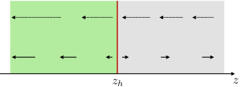
Figure 1: Propagation of monochromatic waves in an optical material whose magnetoelectric coefficient depends on the coordinate $z$, as given by the toy-model set by Eq. (17). Dashed and solid arrows represent the two possible solutions described by Eqs. (15) and (16), respectively. Their sizes are related to the magnitude of the corresponding phase velocities. The vertical line represents the horizon, that is located at $z=z_{h}$.

Solutions of light rays propagating to the right cannot exist in the region given by $z<z_{h}$, since their velocities are negative due to the influence of the magnetoelectric effect. It is interesting to notice that in such region, birefringence occurs, as there will be two modes propagating in a same direction but with different phase velocities. Furthermore, this region ($z<z_{h}$) is a sort of one-way system, as there will be no solution propagating to the right. On the other hand, there is no birefringence in the region given by $z>z_{h}$. In this region the two solutions correspond to rays propagating in opposite directions. However, these solutions correspond to quite different phase velocities, which makes the propagation in this region ($z>z_{h}$) non-symmetric under space reversal. Another interesting aspect is that the region nearby the event horizon ($z\approx z_{h}$) is a sort of slow light region for the mode described by Eq. (16). Its phase velocity is exactly zero at $z=z_{h}$ and increases as it moves away from this region. The very dependence of the magnitude of the velocity with the distance to the analog horizon is certainly dependent on the chosen model, such as the particular one set by Eq. (17), but the fact that its velocity must be zero at $z_{h}$ and is near zero in its immediate vicinity, is not dependent on the specific model, but a consequence of the presence of the horizon.

Closing this section, the implications of assuming a position dependent magnetoelectric coefficient in the analysis of wave propagation must be justified. For a moment, let us assume a general dependence of this coefficient on the coordinate $z$. In this case, it can be shown that considering $\alpha_{ij}(z)$ in Eqs. (6) and (7), leads to

$$ie^{-i(\mathbf{q}\cdot\mathbf{r}-\omega t)}Z_{ij}e_{j}+\epsilon_{ijk}\left[\partial_{j}\alpha_{lk}(z)\right]E_{l}^{0}=0,$$ (18)

where $E_{l}^{0}$ is the applied electric field, and $Z_{ij}$ was derived in Eq. (8). In order to maintain the previous analysis, one should guarantee that the second term in Eq. (18) does not contribute to the effect. Thus, let us treat this term separately in order to find a consistency condition to the validity of our results concerning the analog event horizon.

If we set the external field, for instance, in the $z$ direction, i.e., $E_{l}^{0}=(0,0,E)$, one gets the consistency conditions given by

$$\epsilon_{i3k}(\partial_{z}\alpha_{3k})E=\begin{cases}-\partial_{z}\alpha_{32}=0,\hskip 14.22636pti=1\\ \hskip 8.5359pt\partial_{z}\alpha_{31}=0,\hskip 14.22636pti=2.\end{cases}$$

Therefore, for such a configuration, if one tailor a metamaterial where the coefficients $\alpha_{31}$ and $\alpha_{32}$ are constants, the consistency of the analysis is guaranteed and an analog event horizon characterized by Eq. (16) can in principle be produced in such artificial systems.

V Final remarks

There are different ways of producing formal analogies between light propagation in an optical medium and metric solutions of general relativity. The one which was explored in this paper is based on the description of light propagation in an optical medium through an effective geometric interpretation, as was formally discussed in Sec. II. In such scenario, the optical coefficients of the medium in consideration are related to the metric components of a gravitational analog. Another way is to start with a metric solution of general relativity and relate the modification of the electromagnetic fields in such curved spacetime with the constitutive relations of a hypothetical optical medium. More specifically, in the presence of gravity, the electromagnetic field in the empty space has its properties affected by the curvature of the spacetime. As well known since Einstein’s early publications, the contravariant and covariant forms of the electromagnetic tensor, which are associated by the metric, are related by means of an expression that mimics the constitutive relations of a material medium. The metric components describing a curved spacetime can thus be compared with the susceptibility coefficients that describe an effective optical medium, so that a formal analogy is possible, as it was investigated a long time ago plebanski ; post . One immediate conclusion is that such an analogy requires a linear magnetoelectric medium. In this context, it was recently noticed that the term that plays the role of the magnetoelectric coefficient is antisymmetric gibbons . On the other hand, as shown in Sec. IV, if we start by analysing the propagation of light in a material medium exhibiting a non-symmetric magnetoelectric coefficient, one finds that such a medium mimics a curved spacetime presenting nonzero time-space mixed terms in the metric which depend only on the antisymmetric part of $\alpha_{ij}$, as described by Eq. (13). This is a subtle difference that may have appeared due to the establishment of an equivalence between quantities associated with the antisymmetric electromagnetic field $F_{\mu\nu}$ and generally non-symmetric tensorial quantities related to optical coefficients that characterize a material medium.

As specifically examined in Sec. IV.1, the magnetoelectric effect plays a fundamental role in the production of analog models containing an event horizon. Light propagation in the neighborhood of such analog horizon exhibits a non-symmetric spatial behavior. At one side of the horizon, there will be only one direction in which both wave solutions can propagate. This aspect is similar to the behavior of light propagation in the interior of the Schwarzschild event horizon. In fact, one can notice that the solutions given by Eqs. (15) and (16) are very similar to the solutions for a radial propagation in the Schwarzschild metric, written in the Painleveé-Gullstrand coordinates painleve ; gullstrand . Another point that should be mentioned is that the “interior” of the analog event horizon ($z<z_{h}$ in the toy model) becomes a birefringent system, because the two distinct solutions propagate in the same direction with different phase velocities. Moreover, it is noteworthy that near the horizon one of the solutions behaves as a slow-light mode. It propagates with a phase velocity that gets an arbitrarily small value, the closer it is to the horizon, on either side of it. Additionally, even outside the horizon ($z>z_{h}$), reversing the propagation direction leads to different behaviors of the light rays. This is in fact an expected consequence of the presence of magnetoelectric couplings toyoda . The main aspect behind the event horizon solution was the assumption of a magnetoelectric coupling that depends on position. This behavior can be imagined to be artificially produced by joining parallel layers of linear magnetoelectric materials, where in each layer the magnetoelectric effect occurs with a different magnitude. However, other effects should not be neglected in such a system, as an position-dependent refractive index would be responsible for other physical consequences. This is an issue the deserves further investigation.

Closing, analog models for gravity can also be studied in the context of nonlinear couplings. Generally, if we consider the expansion of the polarization and magnetization vectors in terms of the applied fields, several effects in different orders of magnitude are bond to appear in a optical medium, depending on its physical properties. In such nonlinear systems the applied fields may explicitly appear in the metric components of the corresponding analog model, which can lead to richer scenarios to investigate GR metric solutions. Additionally, it should be mentioned that the approximations implemented in the text to first order effects in the linear magnetoelectric coupling can be partially justified by means of the possible existence of the nonlinear effects. If we had kept second order contribution to the linear coupling, the magnitude of corresponding effects could be of the same order, or even smaller, than those associated with higher order couplings, which would requires further analysis.

- (1) W. Gordon, “Zur lichtfortplanzung nach der relativitätstheorie”, Annalen der Physik, Lpz. 72, 421 (1923).
- (2) T. E. Tamm, “The electrodynamics of anisotropic media in the special theory of relativity”, Zhurnal Russkogo Fiziko-Khimicheskogo Obshchestva, Otdel Fizicheskii 56, 248 (1924).
- (3) J. Plebanski, “Electromagnetic waves in gravitational fields”, Physical Review 118, 1396 (1960).
- (4) S. A. Gutiérrez, A. L. Dudley, J. F. Plebanski, “Signals and discontinuities in general relativistic nonlinear electrodynamics”, Journal of Mathematical Physics 22, 2835 (1981).
- (5) M. Novello, V. A. De Lorenci, J. M. Salim and R. Klippert, “Geometrical aspects of light propagation in nonlinear electrodynamics”, Physical Review D 61, 045001 (2000).
- (6) C. Barceló, S. Liberati and M. Visser, “Analogue gravity from field theory normal modes?”, Classical and Quantum Gravity 18, 3595 (2001).
- (7) I. Carusotto, S. Fagnocchi, A. Recati, R. Balbinot and A. Fabbri, “Numerical observation of Hawking radiation from acoustic black holes in atomic Bose-Einstein condensates”, New Journal of Physics 10, 103001 (2008).
- (8) C. Barceló, S. Liberati and M. Visser, “Analog gravity from Bose-Einstein condensates”, Classical and Quantum Gravity 18, 1137 (2001).
- (9) R. Balbinot and A. Fabbri, “Quantum correlations across the horizon in acoustic and gravitational black holes”, Physical Review D 105, 045010 (2022).
- (10) T. G. Mackay and A. Lakhtakia, “Towards a metamaterial simulation of a spinning cosmic string”, Physics Letters A 374, 2305 (2010).
- (11) C. Barceló, J. E. Sanchez, G. G. Moreno and G. Jannes, “Chronology protection implementation in analogue gravity”, The European Physical Journal C 82, 299 (2022).
- (12) S. W. Hawking, “Chronology protection conjecture”, Physics Review D 46, 603 (1992).
- (13) V. A. De Lorenci and E. S. Moreira, Jr., “Spinning strings, cosmic dislocations, and chronology protection”, Phys. Rev. D 70, 047502 (2004).
- (14) M. Lapine, I. V. Shadrivov, and Y. S. Kivshar, “Colloquium: Nonlinear metamaterials”. Reviews of Modern Physics, 86, 1093 (2014).
- (15) M. Fiebig. “Revival of the magnetoelectric effect”. Journal of Physics D: Applied Physics, 38, 123 (2005).
- (16) J. P. Rivera, “A short review of the magnetoelectric effect and related experimental techniques on single phase (multi-) ferroics”, European Physical Journal B 71, 299 (2009).
- (17) H. Schmid, “On a magnetoelectric classification of materials”, International Journal of Magnetism 4, 337 (1973).
- (18) C. Tabares-Muñoz, J. P. Rivera, A. Bezinges, A. Monnier, and H. Schmid, “Measurement of the quadratic magnetoelectric effect on single crystalline BiFeO3” Japanese Journal of Applied Physics 24, 1051 (1985).
- (19) G. Gibbons and M. Werner, “The gravitational magnetoelectric effect”, Universe 5, 88 (2019).
- (20) V. A. De Lorenci and R. Klippert, “Analogue gravity from electrodynamics in nonlinear media”, Physical Review D 65, 064027 (2002).
- (21) V. A. De Lorenci, “Effective geometry for light traveling in material media”, Physical Review E 65, 026612 (2002).
- (22) V. A. De Lorenci, “Aspects of wave propagation in a nonlinear medium: birefringence and the second-order magnetoelectric coefficients”, Physical Review A 105, 023530 (2022).
- (23) W. G. Unruh, “Experimental black-hole evaporation?”, Physics Review Letters 46, 1351 (1981).
- (24) R. Balbinot, A. Fabbri, S. Fagno and R. Parentani, “Hawking radiation from acoustic black holes, short distance and backreaction effects”, La Rivista del Nuovo Cimento 28, 1 (2005).
- (25) C. Barceló, S. Liberati, and M. Visser, “Analogue gravity”, Living Reviews in Relativity 14, 3 (2011).
- (26) E. J. Post, Formal structure of the electromagnetics (North-Holland, Amsterdam, 1962), Chap. 9.
- (27) P. Painlevé, “La mécanique classique et la théorie de la relativité”, Comptes Rendue de l’Academie de Seances 173, 677 (1921).
- (28) A. Gullstrand, “Allegemeine l orper-problems in der Einsteinshen osung des statischen eink gravitations theorie”, Arkiv för Matematik, Astronomi och Fysik 76, 1 (1922).
- (29) S. Toyoda, N. Abe, and T. Arima, “Nonreciprocal refraction of light in a magnetoelectric material”, Physical Review Letters 123, 077401 (2019).