A matrix–free high–order solver for the numerical solution of cardiac electrophysiology

Abstract

We propose a matrix–free solver for the numerical solution of the cardiac electrophysiology model consisting of the monodomain nonlinear reaction–diffusion equation coupled with a system of ordinary differential equations for the ionic species. Our numerical approximation is based on the high–order Spectral Element Method (SEM) to achieve accurate numerical discretization while employing a much smaller number of Degrees of Freedom than first–order Finite Elements. We combine vectorization with sum–factorization, thus allowing for a very efficient use of high–order polynomials in a high performance computing framework. We validate the effectiveness of our matrix–free solver in a variety of applications and perform different electrophysiological simulations ranging from a simple slab of cardiac tissue to a realistic four–chamber heart geometry. We compare SEM to SEM with Numerical Integration (SEM–NI), showing that they provide comparable results in terms of accuracy and efficiency. In both cases, increasing the local polynomial degree $p$ leads to better numerical results and smaller computational times than reducing the mesh size $h$. We also implement a matrix–free Geometric Multigrid preconditioner that results in a comparable number of linear solver iterations with respect to a state–of–the–art matrix–based Algebraic Multigrid preconditioner. As a matter of fact, the matrix–free solver proposed here yields up to 45$\times$ speed–up with respect to a conventional matrix–based solver.

1 Introduction

Mathematical and numerical modeling of cardiac electrophysiology provides meaningful tools to address clinical problems in silico, ranging from the cellular to the organ scale [1, 2, 3, 4, 5]. For this reason, several mathematical models and methods have been designed to perform electrophysiological simulations [6, 7]. Among these, we consider the monodomain equation coupled with suitable ionic models, which describes the space–time evolution of the transmembrane potential and the flow of chemical species across ion channels [8].

This set of combined partial and ordinary differential equations describes solutions that resemble those of a wavefront propagation problem, i.e. manifesting very steep gradients. Despite being extensively used [9, 10, 11, 12], the Finite Element Method (FEM) with first order polynomials does not seem to be the most suitable to properly capture the physical processes underlying cardiac electrophysiology [13]. Indeed, in such cases, a very fine mesh resolution is required to obtain fully convergent numerical results [14], which calls for an overwhelming computational burden.

High–order numerical methods come into play to tackle this specific issue: Spectral Element Method (SEM) [15, 16, 17], high–order Discontinuous Galerkin (DG) [18, 19], Finite Volume Method (FVM) [20], or Isogeometric Analysis (IGA) [21] account for small numerical dispersion and dissipation errors while allowing for converging numerical solutions with less Degrees of Freedom (DOFs) [22, 23, 24, 25]. However, the use of high–order polynomials in matrix–based solvers for complex scenarios has been hampered by several numerical challenges, which are mostly related to the stiffness of the discretized monodomain problem [26].

In this context, we develop and implement a high–order matrix–free numerical solver that can be readily employed for CPU–based, massively parallel, large–scale numerical simulations. Since there is no need to assemble any matrix, all the floating point operations are associated with matrix–vector products that represent the most demanding computational kernels at each iteration of iterative solvers. Thanks to vectorization [27], which enables algebraic operations on multiple mesh cells at the same time, and sum–factorization [28, 29], the higher the polynomial degree, the higher the computational advantages provided by the matrix–free solver [23, 30]. Moreover, the small memory occupation required by the matrix–free implementation allows for its exploitation in GPU–based cardiac solvers [31, 32, 33].

In this manner, we obtain very accurate and efficient numerical simulations for cardiac electrophysiology, even if the linear solver remains unpreconditioned. Additionally, we implement a matrix–free Geometric Multigrid (GMG) preconditioner that is optimal for the values of $h$ (mesh size) and $p$ (polynomial degree) considered in this paper when continuous model properties (i.e a single ionic model and a continuous set of conductivity coefficients) are employed throughout the computational domain.

We present different benchmark problems of increasing complexity for cardiac electrophysiology, ranging from the Niederer benchmark on a slab of cardiac tissue [34] to a whole–heart numerical simulation. We focus on two high–order discretization methods, namely, we compare SEM to SEM with Numerical Integration (SEM–NI), following the notations introduced in [17]. These two methods differ in the use of quadrature formulas, namely Legendre–Gauss for SEM and Legendre–Gauss–Lobatto for SEM–NI. Numerical results of Section 5 show that the two methods feature a similar behaviour in terms of both accuracy and computational costs. In both cases, choosing a higher polynomial degree $p$ leads to a fairly more beneficial ratio between accuracy and computational costs than reducing the mesh size $h$. For instance, working with two discretizations with the same number of DOFs on the Niederer benchmark, the solution computed with ${\mathbb{Q}}_{4}$ (local polynomials of degree 4 with respect to each spatial coordinate) and average mesh size $h_{\mathrm{avg}}=0.48$ mm is more accurate than the one obtained with ${\mathbb{Q}}_{1}$ and average mesh size $h_{\mathrm{avg}}=0.12$ mm. Moreover, the former one has been computed at a computational cost that is about 40% of the latter one.

We also evaluate the performance of our matrix–free solver: a 45$\times$ speed–up is achieved with respect to the matrix–based solver. Furthermore, while with the matrix–based implementation the assembling and solving phases of the monodomain problem take more than 70% of the total computational time, which also includes the solution of the system of ODEs associated with the coupled ionic models and the evaluation of the ionic current at each time step, plus some negligible initialization stages, this value drops to approximately 20% with the matrix–free solver.

The mathematical models and the numerical methods contained in this paper have been implemented in life^x [35] (https://lifex.gitlab.io/), a high-performance C++ library developed within the iHEART project and based on the deal.II (https://www.dealii.org) Finite Element core [36].

The outline of the paper is as follows. We describe the monodomain model in Section 2. We address its space and time discretizations in Section 3. We propose the matrix–free solver for cardiac electrophysiology and the matrix–free GMG preconditioner in Section 4, discussing details about vectorization, sum–factorization and highlighting similarities and differences between the matrix–based and the matrix–free solvers. Finally, the numerical results in Section 5 demonstrate the high efficiency of our high–order SEM matrix–free solver against the low–order FEM matrix–based one.

2 Mathematical model

For the mathematical modeling of cardiac electrophysiology, we consider the monodomain equation coupled with suitable ionic models [6, 8]:

$$\left\{\begin{array}[]{ll}\displaystyle\chi\left(C_{\mathrm{m}}\frac{\partial u}{\partial t}+{\mathcal{I}_{\mathrm{ion}}}(u,\bm{w},\bm{z})\right)-\nabla\cdot(\bm{D}_{\mathrm{M}}\nabla u)=\chi{\mathcal{I}_{\mathrm{app}}}({\bf x},t),&\mbox{ in }\Omega\times(0,T],\\[5.69054pt] (\bm{D}_{\mathrm{M}}\nabla u)\cdot{\bf n}=0,&\mbox{ on }\partial\Omega\times(0,T],\\[5.69054pt] \displaystyle\frac{d\bm{w}}{dt}=\bm{H}(u,\bm{w},\bm{z}),&\mbox{ in }\Omega\times(0,T],\\[5.69054pt] \displaystyle\frac{d\bm{z}}{dt}=\bm{G}(u,\bm{w},\bm{z}),&\mbox{ in }\Omega\times(0,T],\\[5.69054pt] u({\bf x},0)=u_{0}({\bf x}),\ \bm{w}({\bf x},0)=\bm{w}_{0}({\bf x}),\ \bm{z}({\bf x},0)=\bm{z}_{0}({\bf x}),&\mbox{ in }\Omega.\end{array}\right.$$ (6)

The unknowns are: the transmembrane potential $u$, the vector $\bm{w}=(w_{1},\ldots,w_{M})$ of the probability density functions of $M$ gating variables, which represent the fraction of open channels across the membrane of a single cardiomyocyte, and the vector $\bm{z}=(z_{1},\ldots,z_{P})$ of the concentrations of $P$ ionic species. For the sake of simplifying the notation, in the following the membrane capacitance per unit area $C_{\mathrm{m}}$ and the membrane surface–to–volume ratio $\chi$ are set equal to $1$.

The mathematical expressions of the functions $\bm{H}(u,\bm{w},\bm{z})$ and $\bm{G}(u,\bm{w},\bm{z})$, which describe the dynamics of gating variables and ionic concentrations respectively, and the ionic current ${\mathcal{I}_{\mathrm{ion}}}(u,\bm{w},\bm{z})$ strictly depend on the choice of the ionic model. Here, the TTP06 [37] ionic model is adopted for the slab and ventricular geometries, while the CRN [38] ionic model is employed for the atria. The action potential is triggered by an external applied current ${\mathcal{I}_{\mathrm{app}}}({\bf x},t)$.

The diffusion tensor $\bm{D}_{\mathrm{M}}$ is expressed as follows

$$\bm{D}_{\mathrm{M}}=\sigma_{\text{l}}{\mathbf{f}_{0}}\otimes{\mathbf{f}_{0}}+\sigma_{\text{t}}{\mathbf{s}_{0}}\otimes{\mathbf{s}_{0}}+\sigma_{\text{n}}{\mathbf{n}_{0}}\otimes{\mathbf{n}_{0}},$$ (7)

where the vector fields ${\mathbf{f}_{0}}$, ${\mathbf{s}_{0}}$ and ${\mathbf{n}_{0}}$ express the fiber, the sheetlet and the sheet–normal (cross–fiber) directions, respectively [39, 40]. We also define longitudinal, transversal and normal conductivities as $\sigma_{\text{l}},\sigma_{\text{t}},\sigma_{\text{n}}\in\mathbb{R}^{+}$, respectively [39]. Homogeneous Neumann boundary conditions are prescribed on the whole boundary $\partial\Omega$ to impose the condition of electrically isolated domain, $\mathbf{n}$ being the outward unit normal vector to the boundary.

In this paper, the computational domain $\Omega\subset{\mathbb{R}}^{3}$ is represented either by a slab of cardiac tissue or by the Zygote geometry [41].

3 Space and time discretizations

In order to discretize in space the system (6), we adopt SEM [15, 16, 17, 42, 43], a high-order method that can be recast in the framework of the Galerkin method [13].

We consider a family of hexahedral conforming meshes, satisfying standard assumption of regularity and quasi–uniformity [13], and let $h>0$ denote the mesh size.

At each time, we look for the discrete solution belonging to the space of globally continuous functions that are the tensorial product of univariate piecewise (on each mesh element) polynomial functions of local degree $p\geq 1$ with respect to each coordinate. The local finite element space is referred to as ${\mathbb{Q}}_{p}$, while we denote by $V_{h,p}$ the global finite dimensional space.

When using SEM, the univariate basis functions are of Lagrangian (i.e., nodal) type and their support nodes $x_{i}$ are the Legendre–Gauss–Lobatto quadrature nodes (see, e.g., [44, Ch. 2]), suitably mapped from the reference interval $[-1,1]$ to the local 1D elements.

One of the main features of SEM is that, when the data are smooth enough, the induced approximation error decays more than algebraically fast with respect to the local polynomial degree. Indeed, it is said that SEM features exponential or spectral convergence. At the same time, the convergence with respect to the mesh size $h$ behaves as in FEM. More precisely, if $u\in H^{s}(\Omega)$, with $s>\frac{3}{2}$, denotes the exact solution of a linear second–order elliptic problem in a Lipschitz domain $\Omega$ and $u_{\text{SEM}}\in V_{hp}$ is its SEM approximation, the following error estimate holds

$$\|u-u_{\text{SEM}}\|_{H^{1}(\Omega)}\leq Ch^{\min(p+1,s)-1}p^{1-s}\|u\|_{H^{s}(\Omega)}.$$ (8)

We refer, e.g., to [17, 45] for an experimental support to this estimate.

SEM can be considered as a special case of $hp-$FEM ([43, 46, 47]) with nodal basis functions and conforming hexahedral meshes.

Typically, when using SEM, the integrals appearing in the Galerkin formulation of the differential problem (6) are computed by the composite Legendre–Gauss (LG) quadrature formulas (see [17, 44]). In principle, one can choose LG formulas of the desired order of exactness to guarantee a highly accurate computation of all the integrals appearing in (6). However, a typical choice is to use LG formulas with $(p+1)$ quadrature nodes, which guarantees that the entries of both the mass matrix and the stiffness matrix with constant coefficients are computed exactly while keeping the computational costs not too large [30, 48].

A considerable improvement in reducing the computational times of evaluating the integrals consists of using Legendre–Gauss–Lobatto (LGL) quadrature formulas (instead of LG ones), again with $(p+1)$ nodes that now coincide with the support nodes of the Lagrangian basis functions. This results into the so–called SEM–NI method (NI standing for Numerical Integration). Since the Lagrangian basis functions are mutually orthogonal with respect to the discrete $L^{2}-$inner product induced by the LGL formulas, the mass matrix of the SEM–NI method is diagonal, although not integrated exactly; this is a great strength of SEM–NI in solving time–dependent differential problems through explicit methods when the mass matrix is assembled. On the other hand, as the degree of exactness of LGL quadrature formulas using $(p+1)$ nodes along each direction is $2p-1$, the integrals associated with the nonlinear terms of the differential problem may introduce quadrature errors and aliasing effects that are as significant as the nonlinearities.

We remark that ${\mathbb{Q}}_{1}-$SEM is equivalent to ${\mathbb{Q}}_{1}-$FEM, while ${\mathbb{Q}}_{1}-$SEM–NI is in fact ${\mathbb{Q}}_{1}-$FEM in which the integrals are approximated by the trapezoidal quadrature rule [13].

We choose the same local polynomial degree $p$ (and then the same finite dimensional space) for approximating the transmembrane potential $u$, the gating variables $w_{i}$ (for $i=1,\ldots,M$) and the ionic concentrations $z_{i}$ (for $i=1,\ldots,P$) at each time $t\in(0,T]$.

All the time derivatives appearing in Equation (6) have been approximated using the 2nd–order Backward Differentiation Formula (BDF2) over a discrete set of time steps $t^{n}=n\Delta t,\,n=0,\dots,N$, being $\Delta t$ the time step size.

One may wonder whether the BDF2 scheme is accurate enough for our simulations, even when high-order spatial discretizations (${\mathbb{Q}}_{3}$ and ${\mathbb{Q}}_{4}$ SEM) are used, or if it is better to consider higher order methods like, e.g., the BDF3 scheme. To remove any doubt, we have approximated the heat equation in a two–dimensional domain, with discretization parameters similar to those used in our simulations. We have verified that, with these discretization parameters, the errors in space overbear those in time, thus making the use of BDF3 worthless. Moreover, we remark that, while BDF2 is absolutely stable, BDF3 is not, then special care should be given to the choice of the time step. We refer to A for a more in–depth analysis.

Regardless of the quadrature formula (LG or LGL), the algebraic counterpart of the monodomain problem (6) reads: given $\bm{\mathsf{w}}^{0}$, $\bm{\mathsf{z}}^{0}$ and $\mathsf{u}^{0}$, and suitable initializations for $\bm{\mathsf{w}}^{1}$, $\bm{\mathsf{z}}^{1}$ and $\mathsf{u}^{1}$, then, for any $n\geq 1$, find $\bm{\mathsf{w}}^{n+1}$, $\bm{\mathsf{z}}^{n+1}$ and $\mathsf{u}^{n+1}$ by solving the following partitioned scheme:

$$\left\{\begin{aligned} &\frac{3\bm{\mathsf{w}}^{n+1}-4\bm{\mathsf{w}}^{n}+\bm{\mathsf{w}}^{n-1}}{2\Delta t}=\bm{H}(\mathsf{u}^{*},\bm{\mathsf{w}}^{n+1},\bm{\mathsf{z}}^{n+1}),\\ &\frac{3\bm{\mathsf{z}}^{n+1}-4\bm{\mathsf{z}}^{n}+\bm{\mathsf{z}}^{n-1}}{2\Delta t}=\bm{G}(\mathsf{u}^{*},\bm{\mathsf{w}}^{n+1},\bm{\mathsf{z}}^{n+1}),\end{aligned}\right.$$ (9a)

$$\mathsf{M}\frac{3\mathsf{u}^{n+1}-4\mathsf{u}^{n}+\mathsf{u}^{n-1}}{2\Delta t}+\mathsf{K}\mathsf{u}^{n+1}=\mathsf{s}^{n+1}+\mathsf{f}^{n+1}.$$ (9b)

The arrays $\mathsf{u}^{n+1}$ and $\bm{\mathsf{w}}^{n+1}$ and $\bm{\mathsf{z}}^{n+1}$ contain the SEM or SEM–NI DOFs of the transmembrane potential, gating variables and ionic concentrations, respectively, $\mathsf{M}$ and $\mathsf{K}$ are the SEM or SEM–NI mass and stiffness matrices, respectively, and $\mathsf{f}_{i}^{n+1}={\mathcal{I}_{\mathrm{app}}}({\bf x}_{i},t^{n+1})$. The entries of $\mathsf{s}^{n+1}$ are computed with Ionic Current Interpolation (ICI) [49], i.e.,

$$\mathsf{s}_{i}^{n+1}=-\int_{\Omega}\left(\sum_{j}{\mathcal{I}_{\mathrm{ion}}}(\mathsf{u}_{j}^{*},\bm{\mathsf{w}}_{j}^{n+1},\bm{\mathsf{z}}_{j}^{n+1})\varphi_{j}\right)\varphi_{i},$$ (10)

with $\varphi_{i}$ the $i^{th}$ Lagrange basis function of the finite dimensional space $V_{h,p}$. We remark that, when SEM–NI with LGL quadrature formulas are employed, ICI coincides with Lumped–ICI [50], as the lumping of the SEM mass matrix coincides with the SEM–NI mass matrix.

If we set $\mathsf{u}^{*}=\mathsf{u}^{n+1}$, then we recover the fully implicit BDF2 scheme. Nevertheless, we highlight that the function ${\mathcal{I}_{\mathrm{ion}}}$ is typically strongly nonlinear. To overcome the drawbacks of this nonlinearity, we adopt the extrapolation formula $\mathsf{u}^{*}=2\mathsf{u}^{n}-\mathsf{u}^{n-1}$ of $\mathsf{u}^{n+1}$, that is second–order accurate with respect to $\Delta t$. The resulting semi–implicit scheme is 2nd–order accurate in time when $\Delta t\to 0$ (see, e.g., [51]).

The ordinary differential equations (9a) are associated with the ionic model and provide both the gating variables and the ionic species, while Equation (9b) is the discretization of the monodomain equation and its solution at the generic time step $n\geq 1$ is obtained by solving the linear system

$$\mathsf{A}\mathsf{u}^{n+1}=\mathsf{b}^{n+1},$$ (11)

where

$$\mathsf{A}=\frac{3}{2\Delta t}\mathsf{M}+\mathsf{K},\hskip 28.45274pt\mathsf{b}^{n+1}=\frac{1}{2\Delta t}\mathsf{M}(4\mathsf{u}^{n}-\mathsf{u}^{n-1})+\mathsf{s}^{n+1}+\mathsf{f}^{n+1}.$$ (12)

Solving the linear system (11) represents the most computationally demanding part of Equation (9). We refer to Section 5, in particular to Table 8, for further details about this specific aspect.

4 Matrix–free and matrix–based solvers

As in FEM, the matrix $\mathsf{A}$ based on either SEM or SEM–NI has a very sparse structure, thus iterative methods are the natural candidates to solve the linear system (11). Since $\mathsf{A}$ is symmetric and positive definite, we have adopted the Conjugate Gradient (CG) method or its preconditioned version (PCG).

Excluding the preconditioner step, the most expensive part of one CG–iteration is the evaluation of a matrix–vector product $\mathsf{A}\mathbf{v}$, where $\mathbf{v}$ is a given vector.

Typically, in a conventional matrix–based solver, the matrix $\mathsf{A}$ is assembled and stored in sparse format, then referenced whenever the matrix–vector product has to be evaluated, i.e. during each CG iteration. The matrix–based solver aims at minimizing the number of floating point operations required for such evaluation and is a winning strategy in ${\mathbb{Q}}_{1}-$FEM discretization for which the band of the matrix $\mathsf{A}$ is small.

When SEM or SEM–NI discretizations of local degree $p$ are employed, each cell counts $(p+1)^{3}$ DOFs. It follows that the typical bandwidth of SEM (or SEM–NI) stiffness matrices is about $C(p+1)^{3}$ (where $C$ is the maximum number of cells sharing one node of the mesh) and it exceeds widely that of ${\mathbb{Q}}_{1}-$FEM stiffness matrices. The large bandwidth of the SEM matrix $\mathsf{A}$ can worsen the computational times of accessing the matrix entries, thus deteriorating the efficiency of the iterative solver.

Moreover, in modern processors, access to the main memory has become the bottleneck in many solvers for partial differential equations: a matrix–vector product based on matrices requires far more time waiting for data to arrive from memory than on actually doing the floating point operations. Thus, it is demonstrated to be more efficient to recompute matrix entries – or rather, the action of the differential operator represented by these entries on a known vector, cell by cell – rather than looking up global matrix entries in the memory, even if the former approach requires a significant number of additional floating point operations [30].

This approach is referred to as matrix–free. In practice, shape functions values and gradients are pre-computed for each basis function on the reference cell, for each quadrature node. Then, the Jacobian of the transformation from the real to the reference cell is cached, thus improving the computational cost of the evaluation.

4.1 Vectorization and sum–factorization

In FEM solvers (and, similarly, in SEM ones), the cell–wise computations are typically exactly the same for all cells, and hence a Single–Instruction, Multiple–Data (SIMD) stream can be used to process several values at once (see Figure 1). Vectorization is a SIMD concept, that is, one CPU instruction is used to process multiple cells at once. Modern CPUs support SIMD instruction sets to different extents, i.e. one single CPU instruction can simultaneously process from two doubles (or four floats) up to eight doubles (or sixteen floats), depending on the underlying architecture [52]. Additionally, vectorization can also be combined to a distributed memory parallelism [53]. In our case, the mesh cells and degrees of freedom are partitioned and distributed among different parallel processing units via MPI [54], resulting in the scheme shown in Figure 2.

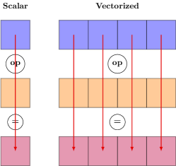
Figure 1: Comparison between scalar and vectorized operations.

(a) Original mesh.

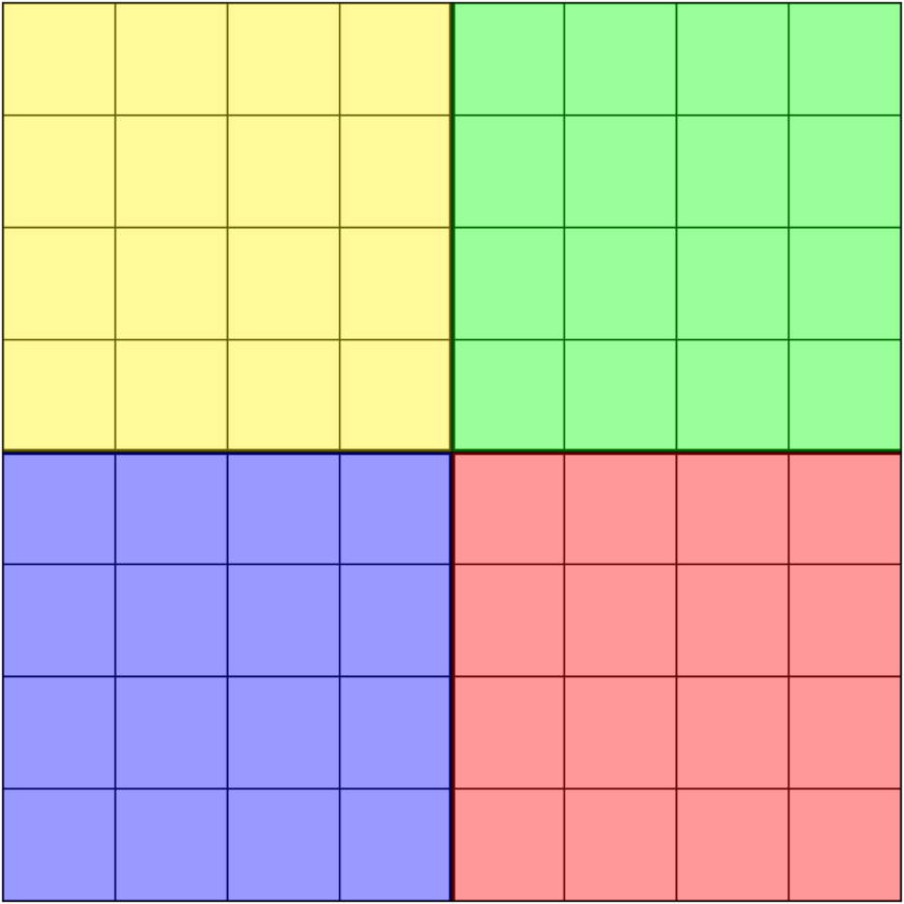
(b) Parallel partitioning of mesh cells. Bold solid lines delimit cells owned by different parallel processors.

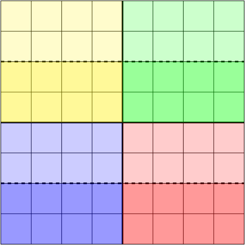
(c) Vectorization of cell operations on each parallel unit. Dashed lines delimit batches of cells processed using vectorized operations, within each processor.

Figure 2: Vectorization in a parallel framework: when the original mesh is partitioned and distributed among multiple computational units, vectorization is applied at the level of each processor (in this example, 4 parallel processors are considered). Here, different colors refer to different parallel units and light/dark variations represent different vectorized batches (in this example, vectorization acts on 8 cells).

Vectorization is beneficial only in arithmetic intensive operations, whereas additional computational power becomes useless when the workload bottleneck is the memory bandwidth. For this reason, vectorization is typically not used explicitly in matrix–based Finite Element codes, whose computational efficiency is dominated by memory access. On the other hand, matrix–free solvers can easily benefit from the additional computational speed–up brought in by vectorized operations. As a matter of fact, in this case a matrix–vector product results from recomputing the local action of the matrix on the vector, cell by cell, every time that it is needed, rather than accessing global matrix entries in the memory. In our matrix–free Algorithm 2, vectorization acts on the cell loop performed at line 1.

Finally, thanks to the fact that the multivariate SEM Lagrange basis is of tensorial type, in order to reduce the computational complexity of one evaluation of the product $\mathsf{A}\mathbf{v}$, sum–factorization can also be exploited [28, 29, 55]. In this way, the matrix–vector product for the Laplace operator in the generic three dimensional cell requires only $9(p+1)$ floating point operations instead of $(p+1)^{3}$ per degree of freedom, resulting in a complexity equal to $\mathcal{O}\left(9(p+1)^{4}\right)$ instead of $\mathcal{O}\left((p+1)^{6}\right)$, and this still plays in favor of repeating computations rather than accessing the memory (see [56, Section 2.3.1] and [44, Section 4.5.1]).

On these bases, a high–order matrix–free solver is more efficient both in terms of memory occupation (no system matrix is assembled and stored globally) and computational time [30], as we will also show in Section 5.

4.2 Application to cardiac electrophysiology

In Algorithms 1 and 2 we display the computational workflow resulting from applying the matrix–free and the matrix–based solver to problem (9), respectively. The different phases are listed. We highlight that the operations needed to solve the ionic model (9a) and to compute ${\mathcal{I}_{\mathrm{ion}}}$ are the same for both algorithms.

In the following, the expression assembly phase will refer to the assembly of the right–hand side, in the case of the matrix–free solver, and to the assembly of both the right–hand side and the system matrix, in the case of the matrix–based solver. On the other hand, the linear solver phase of the matrix–free algorithm encloses also a cell loop for computing the local action of the discretized operator at each CG iteration, which is not required in the matrix–based case.

Finally, we remark that the diffusion tensor $\bm{D}_{\mathrm{M}}$ is evaluated as in Equation (7) at every quadrature point, resulting in $9(p+1)^{3}$ additional memory accesses per cell.

Both Algorithms 1 and 2 are run in parallel as described in the previous section, by distributing all loops over DOFs and cells according to the mesh partitioning. For the sake of simplicity, the application of suitable preconditioners is omitted from the listings. More details on this topic are discussed in the next section.

Input: $\bm{\mathsf{w}}^{0}$, $\bm{\mathsf{z}}^{0}$ and $\mathsf{u}^{0}$, and suitable initializations for $\bm{\mathsf{w}}^{1}$, $\bm{\mathsf{z}}^{1}$ and $\mathsf{u}^{1}$

1 foreach time step $n\geq 1$ do

2       Compute $\mathsf{u}^{*}=2\mathsf{u}^{n}-\mathsf{u}^{n-1}$;

       ;

       Solve the ionic model and compute the ionic current DOF–wise:;

3       foreach DOF $i$ do

4             Solve Eq. (9a) for $\bm{\mathsf{w}}_{i}^{n+1}$ and $\bm{\mathsf{z}}_{i}^{n+1}$;

5             Compute ${\mathcal{I}_{\mathrm{ion}}}_{,i}={\mathcal{I}_{\mathrm{ion}}}(\mathsf{u}_{i}^{*},\bm{\mathsf{w}}_{i}^{n+1},\bm{\mathsf{z}}_{i}^{n+1})$;

6            

7       end foreach

      ;

       Assembly phase: assemble the rhs of Eq. (9b):;

8       foreach mesh cell $K$ do

9             Compute the local right–hand side;

              $\mathsf{b}_{K}=\mathsf{s}_{K}^{n+1}+\mathsf{f}_{K}^{n+1}+\frac{\mathsf{M}_{K}}{2\Delta t}\left(4\mathsf{u}_{K}^{n}-\mathsf{u}_{K}^{n-1}\right)$;

10            

11            Compress $\mathsf{b}_{K}$ into a global right–hand side $\mathsf{b}$;

12            

13       end foreach

      ;

       Solve the monodomain equation $\left(\frac{3}{2\Delta t}\mathsf{M}+K\right)\mathsf{u}^{(n+1)}=\mathsf{b}$;

        as in Eq. (9b) using CG:;

14       foreach CG iteration $m$ until convergence do

15             Determine the new conjugate vector $\mathbf{v}$;

             ;

             foreach mesh cell $K$ ;

              // Vectorized loop.

16             do

17                   Compute the local mass matrix $\mathsf{M}_{K}$;

18                   Evaluate the diffusion tensor $\bm{D}_{\mathrm{M}}$ at quadrature nodes over $K$;

19                   Compute the local stiffness matrix $\mathsf{K}_{K}$;

20                   Compute the local matrix–vector product:;

                    $\mathbf{z}_{K}=\left(\frac{3}{2\Delta t}\mathsf{M}_{K}+\mathsf{K}_{K}\right)\mathbf{v}_{K}$;

21                   Compress the local contribution $\mathbf{z}_{K}$ into a global vector $\mathbf{z}$;

22                  

23             end foreach

            ;

24             Apply the CG steps to $\mathbf{z}$ in order to get the new solution $\mathsf{u}_{m}^{(n+1)}$;

25            

26       end foreach

      ;

27       $\mathsf{u}^{(n+1)}\leftarrow\mathsf{u}_{m}^{(n+1)}$;

28      

29 end foreach

Algorithm 1 Workflow for the matrix–free solver.

Input: $\bm{\mathsf{w}}^{0}$, $\bm{\mathsf{z}}^{0}$ and $\mathsf{u}^{0}$, and suitable initializations for $\bm{\mathsf{w}}^{1}$, $\bm{\mathsf{z}}^{1}$ and $\mathsf{u}^{1}$

1 foreach time step $n\geq 1$ do

2       Compute $\mathsf{u}^{*}=2\mathsf{u}^{n}-\mathsf{u}^{n-1}$;

       ;

       Solve the ionic model and compute the ionic current DOF–wise:;

3       foreach DOF $i$ do

4             Solve Eq. (9a) for $\bm{\mathsf{w}}_{i}^{n+1}$ and $\bm{\mathsf{z}}_{i}^{n+1}$;

5             Compute ${\mathcal{I}_{\mathrm{ion}}}_{,i}={\mathcal{I}_{\mathrm{ion}}}(\mathsf{u}_{i}^{*},\bm{\mathsf{w}}_{i}^{n+1},\bm{\mathsf{z}}_{i}^{n+1})$;

6            

7       end foreach

      ;

       Assembly phase: assemble the global system matrix;

        and right–hand side:;

8       foreach mesh cell $K$ do

9             Compute the local mass matrix $\mathsf{M}_{K}$;

10             Evaluate the diffusion tensor $\bm{D}_{\mathrm{M}}$ at quadrature nodes over $K$;

11             Compute the local stiffness matrix $\mathsf{K}_{K}$;

             ;

12             Compress the local system matrix $\mathsf{A}_{K}=\left(\frac{3}{2\Delta t}\mathsf{M}_{K}+\mathsf{K}_{K}\right)$;

              into a global matrix $\mathsf{A}$;

13             Compress the local right–hand side;

              $\mathsf{b}_{K}=\mathsf{s}_{K}^{n+1}+\mathsf{f}_{K}^{n+1}+\frac{\mathsf{M}_{K}}{2\Delta t}\left(4\mathsf{u}_{K}^{n}-\mathsf{u}_{K}^{n-1}\right)$;

              into a global right–hand side $\mathsf{b}$;

14            

15       end foreach

      ;

16       Solve the monodomain equation $\mathsf{A}\mathsf{u}^{(n+1)}=\mathsf{b}$;

        as in Eq. (9b) using CG;

17      

18 end foreach

Algorithm 2 Workflow for the matrix–based solver.

4.3 A Geometric Multigrid matrix–free preconditioner

In order to precondition the CG method we have chosen Multigrid preconditioners. For the matrix–based solver, the Algebraic Multigrid (AMG) preconditioner [57, 58] turns out to be a very efficient choice. Nevertheless, its implementation requires the explicit knowledge of the entries of the matrix $\mathsf{A}$.

Hybrid multigrid algorithms with matrix–free implementation for high–order discretizations have recently been proposed and discussed in [59, 60]. In particular the methods proposed in [60] combine $h-$coarsening, $p-$coarsening, and AMG on the coarsest level, and they fully exploit the advantages of matrix–free algorithms with sum–factorization for the multigrid smoothers. The matrix assembly at the coarsest level is however required to implement the AMG solver. We refer to [60] for an interesting presentation of hybrid multigrid techniques and of the challenges to face for improving the efficiency of these algorithms.

To overcome the drawback of assembling the matrix $\mathsf{A}$ even at the coarsest level, we have adopted a fully Geometric Multigrid (GMG) preconditioner, more precisely the high–order $h$–multigrid preconditioner [61], which uses $p$–degree interpolation and restriction among geometrically coarsened meshes. GMG methods are among the most efficient solvers for linear systems arising from the discretization of elliptic partial differential equations, offering an optimal complexity $\mathcal{O}(n)$ in the number of unknowns $n$, and they are often used as very efficient preconditioners (see [32, 57, 62, 63] and the literature cited therein).

In the spirit of [30, 32], our GMG implementation relies on the simple yet effective scheme that considers a polynomial variant of the point–Jacobi smoother, namely a Chebyshev method with optimal parameters determined by an eigenvalue estimation based on Lanczos iterations [64]. This choice turns out to be very efficient in a matrix–free context because all its computational kernels, including the smoother and the transfer between different grid levels, are based on matrix–vector products involving suitable collections of mesh cells [64]. In our case, a hierarchical collection of octree meshes is built by the recursive subdivision of each cell into 8 subcells, starting from a coarse mesh $T_{0}$ of size $h_{0}$, as shown in Figure 3. Despite the higher throughput provided by multigrid in single precision [30], due to the high accuracy required by the monodomain problem at hand we decided to evaluate our GMG preconditioner in double precision, consistently with the matrix and vector representations within the CG solver.

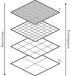
Figure 3: Schematization of multigrid methods in a two dimensional case. Starting from the real mesh $T$, the action of the restriction and prolongation operators is shown, down to the coarse mesh $T_{0}$.

5 Numerical results

We present several numerical simulations of cardiac electrophysiology. First, we consider a benchmark problem on a slab of cardiac tissue [34], in order to compare SEM against SEM–NI and matrix–free against matrix–based in terms of computational efficiency and numerical accuracy. Then, we employ the Zygote left ventricle geometry [41] and we analyze the sole impact of increasing $p$, i.e. the local polynomial degree, on the numerical solution. Finally, for the sake of completeness, we show the capability of our matrix–free solver by presenting a detailed Zygote four–chamber heart [41] electrophysiological simulation in sinus rhythm.

For the time discretization, we use the BDF2 scheme with a time step $\Delta t=$0.1\text{\,}\mathrm{ms}$$. The final time $T$ differs with the specific test case. We employ $T=$0.2\text{\,}\mathrm{s}$$ in the Niederer benchmark [34], while $T=$0.6\text{\,}\mathrm{s}$$ and $T=$0.8\text{\,}\mathrm{s}$$ are considered for the left ventricle and whole–heart geometries, respectively.

For what concerns the GMG–preconditioned CG solver in the matrix–free setting, we estimate the largest eigenvalue $\tilde{\lambda}_{\mathrm{max}}$ for the Chebyshev smoother on each level by performing 10 CG sub–iterations, set the smoothing range to $[0.08\tilde{\lambda}_{\mathrm{max}},1.2\tilde{\lambda}_{\mathrm{max}}]$ (the number 1.2 is a safety factor that allows for some inaccuracies in the eigenvalue estimate) and choose a polynomial degree of 5 (i.e., 5 matrix–-vector products per level and iteration). Besides, for the AMG–preconditioned matrix–based CG solver we rely on the Trilinos ML smoothed aggregation [65], by performing 3 $V$–cycles with polynomial Chebyshev smoother of order $3$ and by setting the aggregation threshold to $10^{-1}$. All the parameters reported above have been empirically determined in order to keep the number of PCG iterations as low as possible.

In all cases the PCG solver is run with a stopping criterion based on the absolute residual with tolerance $10^{-15}$.

To compute the solution at time $t^{n+1}$, we use the solution at time $t^{n}$ as initial guess for the PCG algorithm. Because in our simulations we take a very small $\Delta t$ (tipically $\Delta t=10^{-4}$), the initial guess is itself a good approximation of the solution and a low number of iterations is needed to satisfy the stopping criterion. We have verified that the norm of the starting residual of the linear system is between $10^{-9}$ and $10^{-8}$ along the whole numerical simulation, thus, an absolute stopping test on the residual with tolerance $10^{-15}$ means that we reduce the norm of the residual of about six to seven orders of magnitude.

In the two test cases involving the slab and left ventricle, we employ the GMG (AMG) preconditioner for the matrix–free (matrix–based) solver. On the other hand, no preconditioner is introduced in the four–chamber heart numerical simulation, as the presence of different ionic models in the computational domain, namely the CRN model ([38]) for atria and the TTP06 one ([37]) for ventricles, would make our GMG preconditioner non–optimal in $h$ and $p$.

In Table 1 we report the parameters of the monodomain equation. In particular, the conductivity tensor depends on the fiber distribution as in Equation (7), which is generated by means of the Laplace–Dirichlet Rule–Based Methods proposed in [39, 40].

Variable	Value	Unit	Variable	Value	Unit
Conductivity tensor			Applied current
$\sigma_{\text{l}}$	$0.7643\text{\cdot}{10}^{-4}$	${\mathrm{m}}^{2}\text{\,}{\mathrm{s}}^{-1}$	${\widetilde{\mathcal{I}}_{\mathrm{app}}^{\mathrm{max}}}$	$15$	$\mathrm{V}\text{\,}{\mathrm{s}}^{-1}$
$\sigma_{\text{t}}$	$0.3494\text{\cdot}{10}^{-4}$	${\mathrm{m}}^{2}\text{\,}{\mathrm{s}}^{-1}$	$t_{\mathrm{app}}$	$3\text{\cdot}{10}^{-3}$	$\mathrm{s}$
$\sigma_{\text{n}}$	$0.1125\text{\cdot}{10}^{-4}$	${\mathrm{m}}^{2}\text{\,}{\mathrm{s}}^{-1}$

Table 1: Parameters of the electrophysiology model. The conductivity tensor is defined as in Equation (7). For the CRN and TTP06 ionic models, we adopt the parameters reported in the original papers [37, 38] for epicardial cells.

The external current ${\mathcal{I}_{\mathrm{app}}}({\bf x},t)=\widetilde{\mathcal{I}}_{\mathrm{app}}^{\mathrm{max}}$ is applied for $t\in(0,t_{\mathrm{app}}]$ in a cuboid for the Niederer benchmark (as described in [34]), otherwise in different spheres for the ventricle and whole–heart test cases (we can deduce them from the numerical results shown in Figures 4, 10 and 14).

All the numerical simulations were performed by using one cluster node endowed with 56 cores (two Intel Xeon Gold 6238R, 2.20 GHz), which is available at MOX, Dipartimento di Matematica, Politecnico di Milano.

5.1 Slab of cardiac tissue

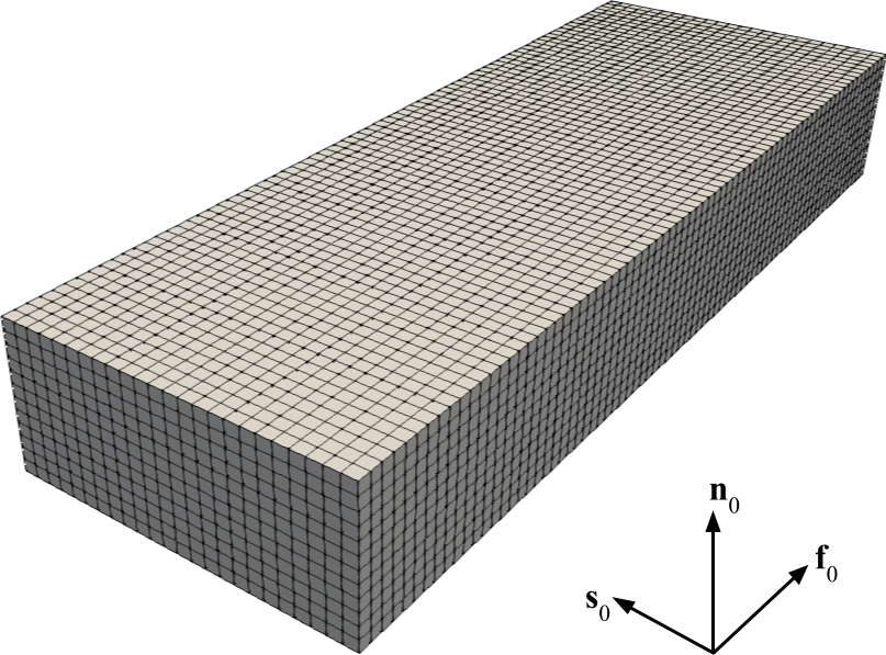
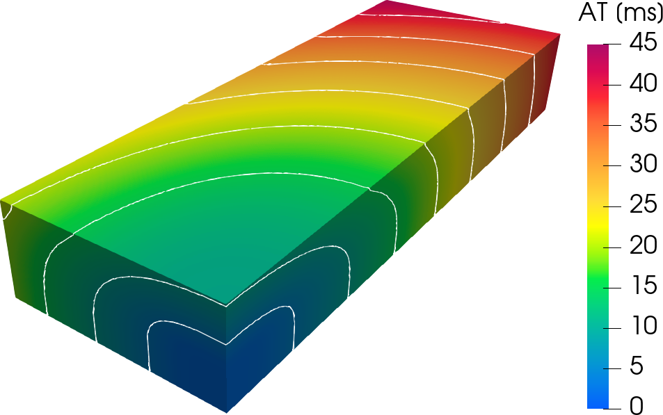
Figure 4: Niederer benchmark. The geometry with the corresponding fiber, sheetlet and cross–fiber orientations and an example of mesh (left) and the associated simulated activation map (right). The blue color represents the region where the cubic stimulus is initially applied; the red one is associated with the corresponding diagonally opposite vertex, which is activated as last.

The computational domain with an example of mesh (left) and the associated numerical simulation (right) for the Niederer benchmark [34] is depicted in Figure 4. An external stimulus of cubic shape is applied at one vertex, the electric signal propagates through the slab, and the diagonally opposite vertex is activated as the last point. The domain is discretized by means of a structured, uniform hexahedral mesh.

We present a systematic comparison between SEM and SEM–NI for several values of both the mesh size $h$ and the local polynomial degree $p$, in order to understand which is the best formulation in terms of accuracy and computational cost. Moreover, we compare the efficiency of the matrix–free and matrix–based solvers for SEM.

In Figures 5 and 6 we show the action potential and the calcium concentration computed with SEM and SEM–NI, respectively, over time. More precisely, the minimum, average, maximum and point values are plotted, where the $\max$, $\min$, and $\mathrm{mean}$ functions are evaluated on the set of nodes of the mesh. We notice that the convergence is faster for increasing $p$ rather than for vanishing $h$.

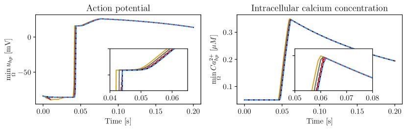
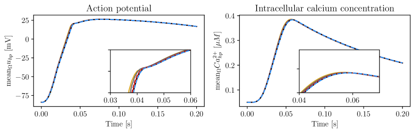
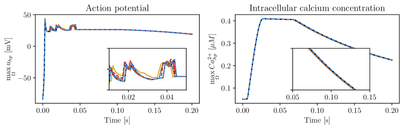
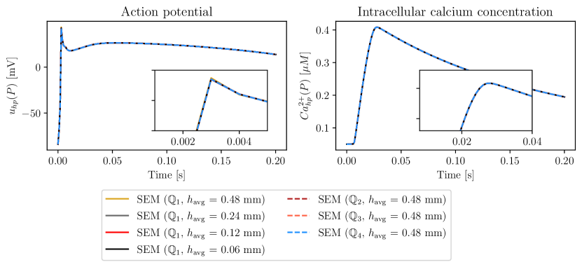
Figure 5: Niederer benchmark. Minimum (top), average (second), maximum (third) and point values (bottom) of the action potential $u$ and intracellular calcium concentration $Ca^{2+}$ over time for a slab of cardiac tissue. $P$ is a random point within the computational domain away from the initial stimulus. We consider different $hp$ combinations: SEM ${\mathbb{Q}}_{1}$ to ${\mathbb{Q}}_{4}$ and $h_{\mathrm{avg}}=$0.48\text{\,}\mathrm{mm}$$ to $h_{\mathrm{avg}}=$0.06\text{\,}\mathrm{mm}$$ ($h_{\mathrm{avg}}$ is the average mesh size).

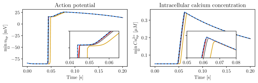
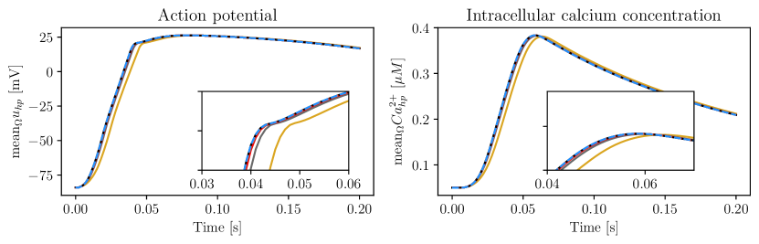
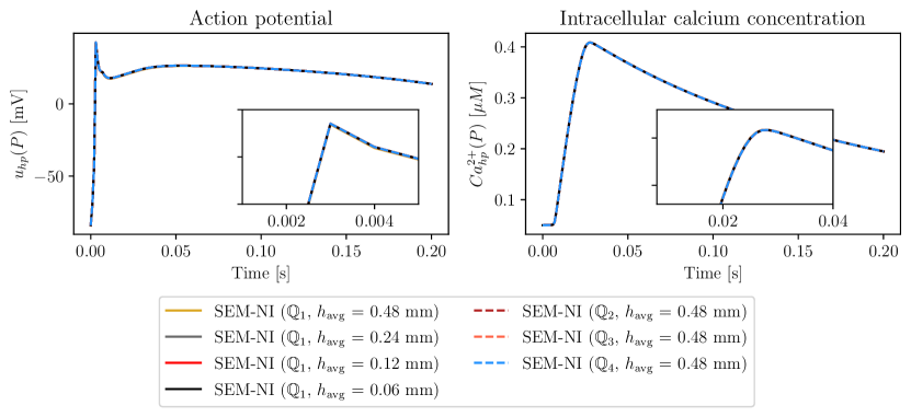
Figure 6: Niederer benchmark. Minimum (top), average (second), maximum (third) and point values (bottom) of the action potential $u$ and intracellular calcium concentration $Ca^{2+}$ over time for a slab of cardiac tissue. $P$ is a random point within the computational domain away from the initial stimulus. We consider different $hp$ combinations: SEM-NI ${\mathbb{Q}}_{1}$ to ${\mathbb{Q}}_{4}$ and $h_{\mathrm{avg}}=$0.48\text{\,}\mathrm{mm}$$ to $h_{\mathrm{avg}}=$0.06\text{\,}\mathrm{mm}$$ ($h_{\mathrm{avg}}$ is the average mesh size).

At each node ${\bf x}_{i}$ of the mesh, we also compute the activation time $\tau$ as the time instant when the approximation of the transmembrane potential $u$ exhibits maximum derivative, i.e.

$$\tau\left(\mathbf{x}_{i}\right)=\operatorname*{arg\,max}_{t}\left|\frac{\partial u}{\partial t}\left(\mathbf{x}_{i},t\right)\right|.$$ (13)

In the formula above $t$ spans over the discrete set of time steps and the time derivative is approximated via the same scheme used for the time discretization of problem (6).

In Figure 7 we show the activation times along the slab diagonal, for different choices of the local space (from ${\mathbb{Q}}_{1}$ to ${\mathbb{Q}}_{4}$) and mesh refinements. As the error accumulates over the diagonal, the inset plots show a zoom around the right endpoint. Such results demonstrate that high polynomial degrees $p$, even with a coarse mesh size $h$, lead to a faster convergence rate compared to the small–$p$, small–$h$ scenario.

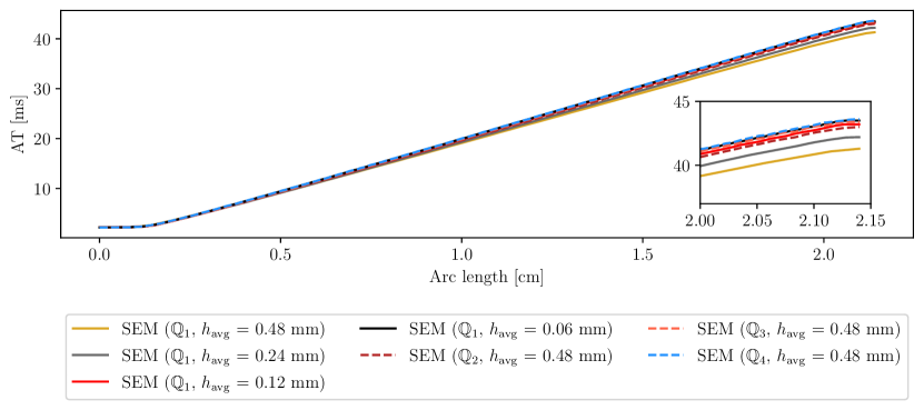
(a) SEM.

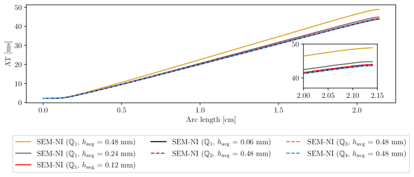
(b) SEM–NI.

Figure 7: Niederer benchmark. Activation times computed along the diagonal of the slab (see Figure 4), with different choices of the local space (${\mathbb{Q}}_{1}$ to ${\mathbb{Q}}_{4}$) and mesh refinements ($h_{\mathrm{avg}}=$0.48\text{\,}\mathrm{mm}$$ to $h_{\mathrm{avg}}=$0.06\text{\,}\mathrm{mm}$$).

To better investigate the comparison between SEM and SEM–NI, in Figure 8 we show the quantities

$$\mathrm{err}_{\max} =\left(\Delta t\sum_{n}\left|\max_{{\bf x}}u_{hp}({\bf x},t_{n})-\max_{{\bf x}}u_{\mathrm{ref}}({\bf x},t_{n})\right|^{2}\right)^{1/2}$$ (14a)

$$\mathrm{err}_{\min} =\left(\Delta t\sum_{n}\left|\min_{{\bf x}}u_{hp}({\bf x},t_{n})-\min_{{\bf x}}u_{\mathrm{ref}}({\bf x},t_{n})\right|^{2}\right)^{1/2}$$ (14b)

$$\mathrm{err}_{\operatorname*{mean}} =\left(\Delta t\sum_{n}\left|\operatorname*{mean}_{{\bf x}}u_{hp}({\bf x},t_{n})-\operatorname*{mean}_{{\bf x}}u_{\mathrm{ref}}({\bf x},t_{n})\right|^{2}\right)^{1/2}$$ (14c)

$$\mathrm{err}_{P} =\left(\Delta t\sum_{n}\left|u_{hp}(P,t_{n})-u_{\mathrm{ref}}(P,t_{n})\right|^{2}\right)^{1/2}$$ (14d)

versus the total number of mesh points, for both the fully discrete SEM and SEM–NI solutions $u_{hp}$. Our reference solution $u_{\mathrm{ref}}$ has been computed with ${\mathbb{Q}}_{4}-$SEM on a grid with average mesh size $h_{\mathrm{avg}}=$0.24\text{\,}\mathrm{mm}$$, for a total of $11^{\prime}401^{\prime}089$ mesh points. $P$ is a random point within the computational domain away from the initial stimulus. The $\max$, $\min$, and $\mathrm{mean}$ functions are evaluated on the set of nodes of the mesh. The number of mesh points increases by reducing $h$ for both “SEM $h$” and “SEM–NI $h$”, while it increases with $p$ for both “SEM $p$” and “SEM–NI $p$”. The numerical results confirm the typical behaviour of SEM and SEM–NI discretizations, i.e. the errors decrease faster by increasing $p$ rather than by decreasing $h$. Moreover, we notice that SEM and SEM–NI errors behave quite similarly, with a slight advantage for SEM.

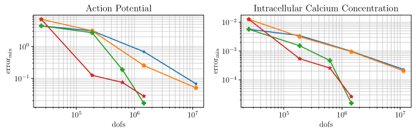
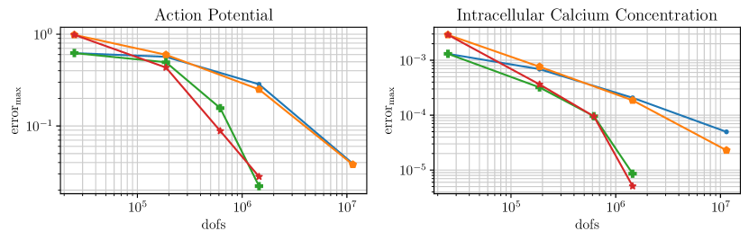
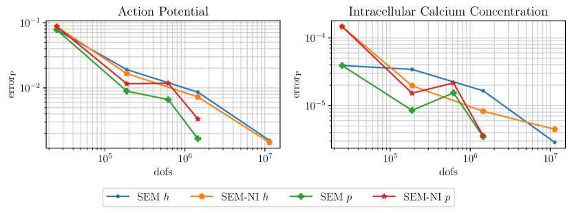
Figure 8: Niederer benchmark. Errors for action potential $u$ and intracellular calcium concentration $Ca^{2+}$ versus the number of mesh points (DOFs) used in a slab of cardiac tissue.

In Tables 2–5 we report the CPU time required by the linear solver for the whole numerical simulation (the times are cumulative over all time steps), for SEM and SEM–NI discretizations, matrix–free and matrix–based solvers. We refer to Section 4.2 for the details of the different algorithmic phases. Furthermore, in Figure 9 we plot the errors (14) versus the CPU time required to solve all the linear systems along the whole numerical simulation. For SEM–NI we only report the times relative to the matrix–free solver, while for SEM we report the times for both the matrix–free and matrix–based solvers. The same symbol (circle, square, diamond, and cross) refers to the numerical simulations carried out on the meshes with the same number of DOFs. If we compare the errors and the CPU–times of ${\mathbb{Q}}_{1}-$SEM, $h_{\mathrm{avg}}=$0.12\text{\,}\mathrm{mm}$$ with those of ${\mathbb{Q}}_{4}-$SEM, $h_{\mathrm{avg}}=$0.48\text{\,}\mathrm{mm}$$ (these two configurations share the same number $1^{\prime}449^{\prime}665$ of mesh nodes), we notice that the errors of ${\mathbb{Q}}_{4}-$SEM are at most about 1/3 – 1/2 of that of ${\mathbb{Q}}_{1}-$SEM and the ratio between the corresponding CPU times is about 40%. Thus, we conclude that ${\mathbb{Q}}_{4}-$SEM outperforms ${\mathbb{Q}}_{1}-$SEM (that is ${\mathbb{Q}}_{1}-$FEM).

Mesh points number	Cells number	Local space	Linear solver SEM [$\mathrm{s}$]	Linear solver SEM–NI [$\mathrm{s}$]	Assemble rhs SEM [$\mathrm{s}$]	Assemble rhs SEM–NI [$\mathrm{s}$]
$25^{\prime}025$	$21^{\prime}888$	$\mathbb{Q}_{1}$	10.769	8.031	0.784	0.766
$187^{\prime}425$	$21^{\prime}888$	$\mathbb{Q}_{2}$	14.694	12.383	4.710	4.645
$618^{\prime}529$	$21^{\prime}888$	$\mathbb{Q}_{3}$	37.733	36.419	14.867	14.542
$1^{\prime}449^{\prime}665$	$21^{\prime}888$	$\mathbb{Q}_{4}$	91.380	90.370	33.899	32.920

Table 2: Niederer benchmark. Computational times for SEM and SEM–NI, with a fixed average mesh size $h_{\mathrm{avg}}=$0.48\text{\,}\mathrm{mm}$$ and $p$ ranging from 1 to 4. Matrix–free solver.

Mesh points number	Cells number	$h_{\mathrm{avg}}$ [$\mathrm{mm}$]	Linear solver SEM [$\mathrm{s}$]	Linear solver SEM–NI [$\mathrm{s}$]	Assemble rhs SEM [$\mathrm{s}$]	Assemble rhs SEM–NI [$\mathrm{s}$]
$25^{\prime}025$	$21^{\prime}888$	0.48	10.769	8.031	0.784	0.766
$187^{\prime}425$	$175^{\prime}104$	0.24	29.157	27.951	5.771	5.656
$1^{\prime}449^{\prime}665$	$1^{\prime}400^{\prime}832$	0.12	256.295	270.959	42.783	43.548
$11^{\prime}401^{\prime}089$	$11^{\prime}206^{\prime}656$	0.06	2137.329	2158.751	336.272	336.641

Table 3: Niederer benchmark. Computational times for SEM and SEM–NI, with an average mesh size $h_{\mathrm{avg}}$ ranging from $0.48\text{\,}\mathrm{mm}$ to $0.06\text{\,}\mathrm{mm}$ and $p$ = 1. Matrix–free solver.

Mesh points number	Cells number	Local space	Linear solver matrix–free [$\mathrm{s}$]	Assembly phase matrix–free [$\mathrm{s}$]	Linear solver matrix–based [$\mathrm{s}$]	Assembly phase matrix–based [$\mathrm{s}$]
$25^{\prime}025$	$21^{\prime}888$	$\mathbb{Q}_{1}$	10.769	0.784	4.086	18.076
$187^{\prime}425$	$21^{\prime}888$	$\mathbb{Q}_{2}$	14.694	4.710	44.200	180.705
$618^{\prime}529$	$21^{\prime}888$	$\mathbb{Q}_{3}$	37.733	14.867	343.243	963.549
$1^{\prime}449^{\prime}665$	$21^{\prime}888$	$\mathbb{Q}_{4}$	91.380	33.899	1557.144	3874.602

Table 4: Niederer benchmark. Computational times for matrix–free and matrix–based solvers, SEM ${\mathbb{Q}}_{p}$ with a fixed average mesh size $h_{\mathrm{avg}}=$0.48\text{\,}\mathrm{mm}$$ and $p$ ranging from 1 to 4.

Mesh points number	Cells number	$h_{\mathrm{avg}}$ [$\mathrm{mm}$]	Linear solver matrix–free [$\mathrm{s}$]	Assembly phase matrix–free [$\mathrm{s}$]	Linear solver matrix–based [$\mathrm{s}$]	Assembly phase matrix–based [$\mathrm{s}$]
$25^{\prime}025$	$21^{\prime}888$	0.48	10.769	0.784	4.086	18.076
$187^{\prime}425$	$175^{\prime}104$	0.24	29.157	5.771	15.373	145.244
$1^{\prime}449^{\prime}665$	$1^{\prime}400^{\prime}832$	0.12	256.295	42.783	204.809	1171.724
$11^{\prime}401^{\prime}089$	$11^{\prime}206^{\prime}656$	0.06	2137.329	336.272	1867.746	9266.635

Table 5: Niederer benchmark. Computational times for matrix–free and matrix–based, SEM ${\mathbb{Q}}_{1}$ with an average mesh size $h_{\mathrm{avg}}$ ranging from $0.48\text{\,}\mathrm{mm}$ to $0.06\text{\,}\mathrm{mm}$.

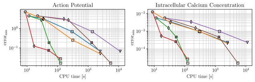
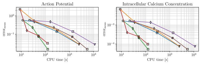
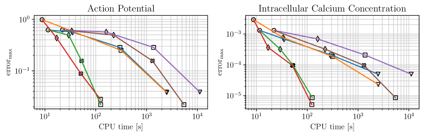
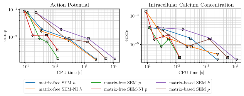
Figure 9: Niederer benchmark. Errors of action potential $u$ and intracellular calcium concentration $Ca^{2+}$ versus CPU time required to solve all the linear systems in a slab of cardiac tissue. Equal symbols identify the same number of mesh points: $\circ$ $25^{\prime}025$, $\diamondsuit$ $187^{\prime}425$, $\times$ $618^{\prime}529$, $\Box$ $1^{\prime}449^{\prime}665$, $\triangledown$ $11^{\prime}401^{\prime}089$.

For the comparison between matrix–free and matrix–based solvers, we notice that the former one is always faster, and the gain of matrix–free over matrix–based solver increases with the polynomial degree $p$. More precisely, the speed–up factors are shown in Table 6 when $h_{\mathrm{avg}}=$0.48\text{\,}\mathrm{mm}$$, and in Table 7 when $p=1$.

Local space	${\mathbb{Q}}_{1}$	${\mathbb{Q}}_{2}$	${\mathbb{Q}}_{3}$	${\mathbb{Q}}_{4}$
$\displaystyle\frac{\mathrm{(CPU\ time)}_{\mathrm{mb}}}{\mathrm{(CPU\ time)}_{\mathrm{mf}}}$	$\sim 2$	$\sim 12$	$\sim 25$	$\sim 45$

Table 6: Niederer benchmark. Speed–up of the matrix–free solver over the matrix–based one when $h_{\mathrm{avg}}=$0.48\text{\,}\mathrm{mm}$$.

$h_{\mathrm{avg}}$	0.48	0.24	0.12	0.06
$\displaystyle\frac{\mathrm{(CPU\ time)}_{\mathrm{mb}}}{\mathrm{(CPU\ time)}_{\mathrm{mf}}}$	$\sim 2$	$\sim 5$	$\sim 5$	$\sim 5$

Table 7: Niederer benchmark. Speed–up of the matrix–free solver over the matrix–based one when $p=1$.

Moreover, from Table 8 we observe that, in a matrix–based electrophysiological simulation, most of the computational time is spent to solve the linear system associated with the monodomain equation. On the contrary, in the matrix–free solver most of the computational time is devoted to the ionic model. This means that the cost for solving the linear system has been highly optimized.

Solver	Monodomain solver	Monodomain assembly	Ionic model solver
Matrix–based ($\mathbb{Q}_{1}$, $h_{\mathrm{avg}}=$0.12\text{\,}\mathrm{mm}$$)	10.54 %	60.41 %	29.05 %
Matrix–free ($\mathbb{Q}_{4}$, $h_{\mathrm{avg}}=$0.48\text{\,}\mathrm{mm}$$)	14.95 %	3.36 %	81.69 %

Table 8: Niederer benchmark. Matrix–free and matrix–based percentages for the assembling and solving phases. Note that in the matrix–free case we only need to assemble the right–hand side vector, as there is no matrix. Moreover, these percentages are computed without taking into account all other phases of the numerical simulation, such as mesh allocation, fiber generation and output of the results.

Finally, we compare the performance of the AMG and GMG preconditioners, used by the matrix–based and matrix–free solvers, respectively. In Tables 9 and 10 we show the average number of iterations required by the PCG method to solve the linear system (11) for different combinations of $h$ and $p$. We notice that, for the values of $h$ and $p$ considered here, both the AMG and GMG preconditioners appear to be optimal in the number of PCG iterations versus both $h$ and $p$. As a matter of fact, the average number of iterations is about 1.0 (matrix–based) and 1.8 (matrix–free) for all $hp$ configurations. More precisely, the number of iterations throughout all the simulations ranges from 1 to 4.

Mesh points number	Cells number	Local space	Matrix–free (SEM) GMG preconditioner	Matrix–free (SEM–NI) GMG preconditioner	Matrix–based (SEM) AMG preconditioner
$25^{\prime}025$	$21^{\prime}888$	$\mathbb{Q}_{1}$	1.6362	1.8126	0.9780
$187^{\prime}425$	$21^{\prime}888$	$\mathbb{Q}_{2}$	1.8056	1.8581	1.0025
$618^{\prime}529$	$21^{\prime}888$	$\mathbb{Q}_{3}$	1.7906	1.8161	1.0205
$1^{\prime}449^{\prime}665$	$21^{\prime}888$	$\mathbb{Q}_{4}$	1.7371	1.7826	1.0250

Table 9: Niederer benchmark. Average number of CG iterations for matrix–free (SEM, SEM–NI) and matrix–based (SEM) solvers, ${\mathbb{Q}}_{p}$ with a fixed average mesh size $h_{\mathrm{avg}}=$0.48\text{\,}\mathrm{mm}$$ and $p$ ranging from 1 to 4.

Mesh points number	Cells number	$h_{\mathrm{avg}}$ [$\mathrm{mm}$]	Matrix–free (SEM) GMG preconditioner	Matrix–free (SEM–NI) GMG preconditioner	Matrix–based (SEM) AMG preconditioner
$25^{\prime}025$	$21^{\prime}888$	0.48	1.6362	1.8126	0.9780
$187^{\prime}425$	$175^{\prime}104$	0.24	1.5757	1.6847	0.9855
$1^{\prime}449^{\prime}665$	$1^{\prime}400^{\prime}832$	0.12	1.4448	1.5937	1.0060
$11^{\prime}401^{\prime}089$	$11^{\prime}206^{\prime}656$	0.06	1.4468	1.4923	1.0180

Table 10: Niederer benchmark. Average number of CG iterations for matrix–free (SEM, SEM–NI) and matrix–based (SEM) solvers, ${\mathbb{Q}}_{1}$ with an average mesh size $h_{\mathrm{avg}}$ ranging from $0.48\text{\,}\mathrm{mm}$ to $0.06\text{\,}\mathrm{mm}$.

The numerical results shown in this section highlight how much advantageous the matrix–free solver with SEM or SEM–NI is for cardiac electrophysiology simulations, with respect to the matrix–based solver with low–order FEM.

Since the matrix–free implementation outperforms the matrix–based one, while SEM and SEM–NI provide comparable results in terms of accuracy and efficiency, we will employ the matrix–free solver with just the SEM formulation for the numerical simulations that we are going to present in the next sections.

5.2 Left ventricle

We report the results for the electrophysiological simulations performed with the Zygote left ventricle geometry [41]. The settings of this test case are summarized at the beginning of Section  5. We consider a mesh with $h_{\mathrm{avg}}=$2.0\text{\,}\mathrm{mm}$$ and polynomial degree $p$ from 1 to 4. In all cases, we keep the mesh boundary fixed to the one resulting from a linear mapping to neglect the impact of boundary deformation on the accuracy of the numerical simulations.

In Table 11 we report the number of mesh nodes, the number of cells and the average number of iterations required by the PCG method to solve the linear system (11). As for the Niederer benchmark, the GMG preconditioner turns out to be optimal also for these numerical simulations. Indeed, the number of PCG iterations is about 2 along the whole time history for any polynomial degree between 1 and 4.

Mesh points number	Cells number	Local space	PCG iterations GMG preconditioner
$159^{\prime}149$	$139^{\prime}684$	$\mathbb{Q}_{1}$	2.0770
$1^{\prime}172^{\prime}919$	$139^{\prime}684$	$\mathbb{Q}_{2}$	1.9628
$3^{\prime}879^{\prime}415$	$139^{\prime}684$	$\mathbb{Q}_{3}$	1.9455
$9^{\prime}116^{\prime}741$	$139^{\prime}684$	$\mathbb{Q}_{4}$	1.9440

Table 11: Zygote left ventricle. Average number of PCG iterations for the matrix–free solver with SEM discretization, ${\mathbb{Q}}_{p}$ with a fixed average mesh size $h_{\mathrm{avg}}=$2.0\text{\,}\mathrm{mm}$$ and $p$ ranging from 1 to 4.

In Figure 10 we depict the activation maps for different choices of the local space (from ${\mathbb{Q}}_{1}$ to ${\mathbb{Q}}_{4}$). By looking at the contour lines, we observe that the ${\mathbb{Q}}_{3}$ solution is very close to the ${\mathbb{Q}}_{4}$ solution, that means we reach convergence for $p=3$, even with such a relatively low mesh resolution $h_{\mathrm{avg}}=$2.0\text{\,}\mathrm{mm}$$. Whereas, it is a well–established result in the literature that first order Finite Elements would reach convergence for a value of $h_{\mathrm{avg}}$ that is about $100$ times smaller – i.e. for a much higher number of DOFs (see, e.g., [14]). We remark that here “DOFs” refers to the number of degrees of freedom associated with the action potential, disregarding both gating variables and ionic species, thus it coincides with the number of mesh nodes. The same conclusions hold when considering Figure 11, where we show the minimum, average, and maximum pointwise values of both the action potential $u$ and the intracellular calcium concentration $Ca^{2+}$ over time.

To further verify these conclusions, we consider different combinations of $h$ and $p$ that lead to the same number of DOFs, namely $9^{\prime}116^{\prime}741$ for $\mathbb{Q}_{1}$ with $h_{\mathrm{avg}}=$0.5\text{\,}\mathrm{mm}$$, $\mathbb{Q}_{2}$ with $h_{\mathrm{avg}}=$1.0\text{\,}\mathrm{mm}$$ and $\mathbb{Q}_{4}$ with $h_{\mathrm{avg}}=$2.0\text{\,}\mathrm{mm}$$. The activation maps displayed in Figure 12 and the pointwise values of the action potential and intracellular calcium shown in Figure 13 reveal that all the results are quite similar and pretty close to convergence, with the $\mathbb{Q}_{4}$ simulation still being the most accurate. Table 12 summarizes the parameters and the computational times recorded for the three simulations, which have been performed with the matrix–free solver and the SEM formulation. Going from $\mathbb{Q}_{1}$ to $\mathbb{Q}_{4}$, the time spent in solving the linear system is reduced of about 9%, whereas the cost of assembling the right–hand side is reduced of about 50%, leading to an overall reduction of about 12%. These results further confirm that in the matrix–free context the strategy of increasing $p$ rather than reducing $h$ is more advantageous in terms of both numerical accuracy and computational efficiency.

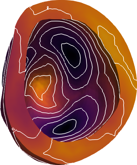
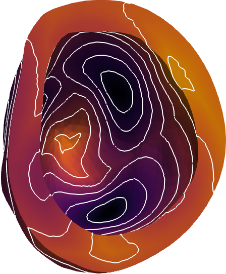
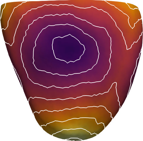
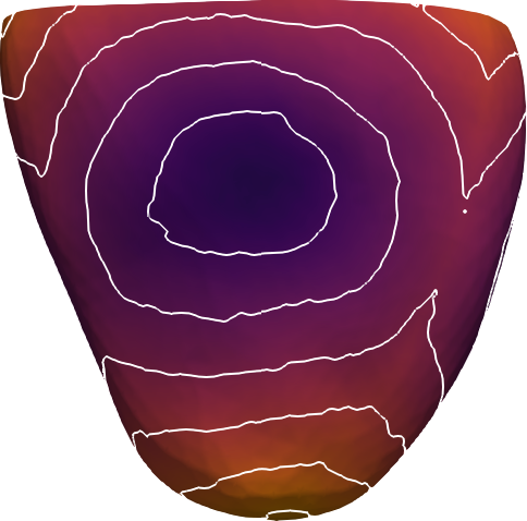
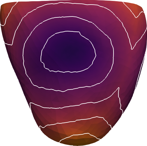
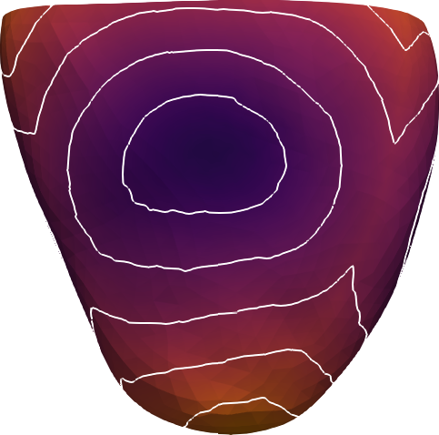
$159^{\prime}149\,\,\text{DOFs}$
($\mathbb{Q}_{1}$)

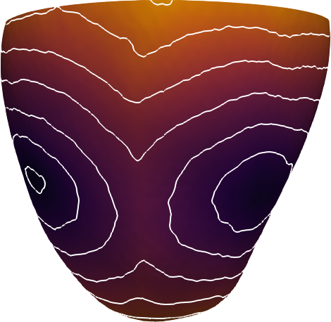
$1^{\prime}172^{\prime}919\,\,\text{DOFs}$
($\mathbb{Q}_{2}$)

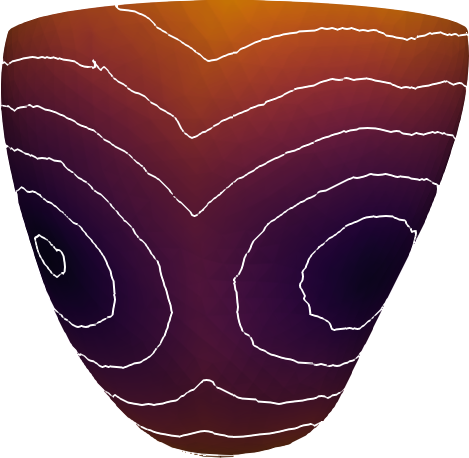
$3^{\prime}879^{\prime}415\,\,\text{DOFs}$
($\mathbb{Q}_{3}$)

$9^{\prime}116^{\prime}741\,\,\text{DOFs}$
($\mathbb{Q}_{4}$)

Figure 10: Zygote left ventricle. Three views of the activation maps computed with ${\mathbb{Q}}_{p}$ elements ($p=1,\dots,4$) and a fixed average mesh size $h_{\mathrm{avg}}=$2.0\text{\,}\mathrm{mm}$$.

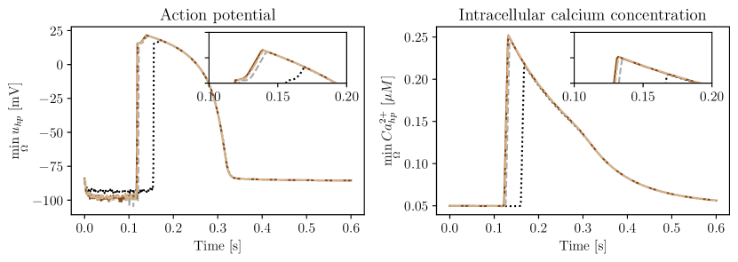
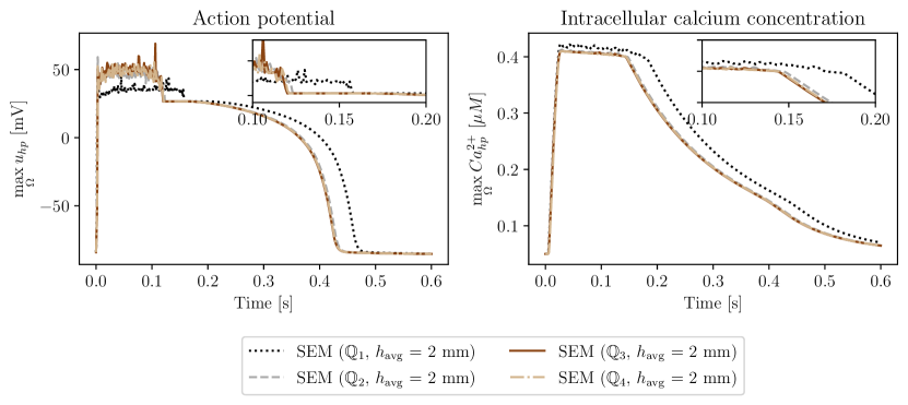
Figure 11: Zygote left ventricle. Minimum (top), average (mid), maximum (bottom) pointwise values of action potential $u$ and intracellular calcium concentration $Ca^{2+}$ over time, ${\mathbb{Q}}_{p}$ with a fixed average mesh size $h_{\mathrm{avg}}=$2.0\text{\,}\mathrm{mm}$$ and $p$ ranging from 1 to 4.

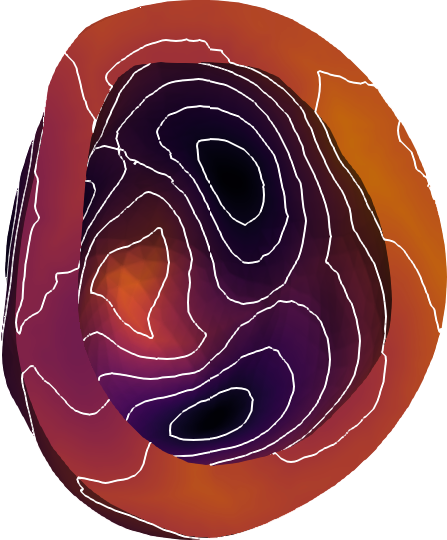
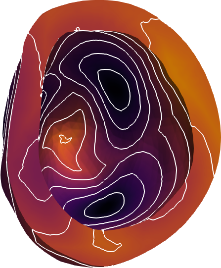
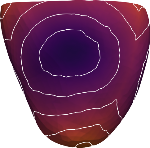
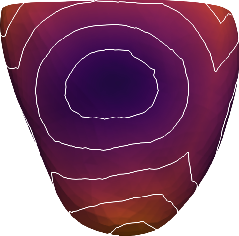
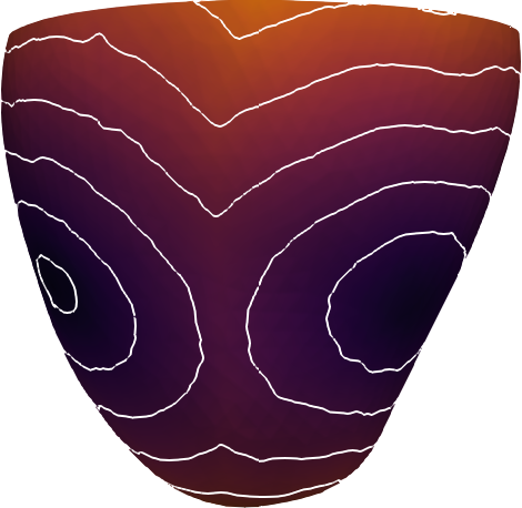
$9^{\prime}116^{\prime}741\,\,\text{DOFs}$
($\mathbb{Q}_{1}$, $h_{\mathrm{avg}}=$0.5\text{\,}\mathrm{mm}$$)

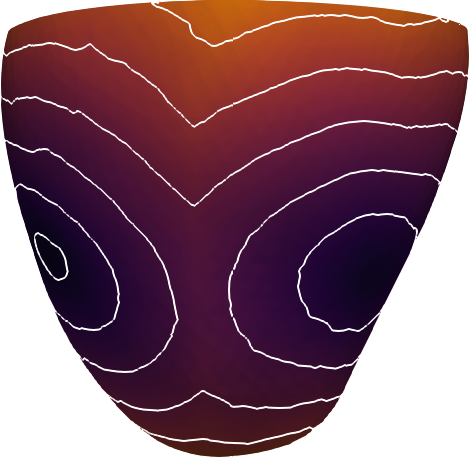
$9^{\prime}116^{\prime}741\,\,\text{DOFs}$
($\mathbb{Q}_{2}$, $h_{\mathrm{avg}}=$1.0\text{\,}\mathrm{mm}$$)

$9^{\prime}116^{\prime}741\,\,\text{DOFs}$
($\mathbb{Q}_{4}$, $h_{\mathrm{avg}}=$2.0\text{\,}\mathrm{mm}$$)

Figure 12: Zygote left ventricle. Three views of the activation maps computed with ${\mathbb{Q}}_{1},{\mathbb{Q}}_{2},{\mathbb{Q}}_{4}$ elements and a fixed number of DOFs equal to $9^{\prime}116^{\prime}741$.

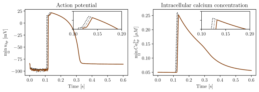
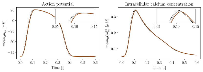
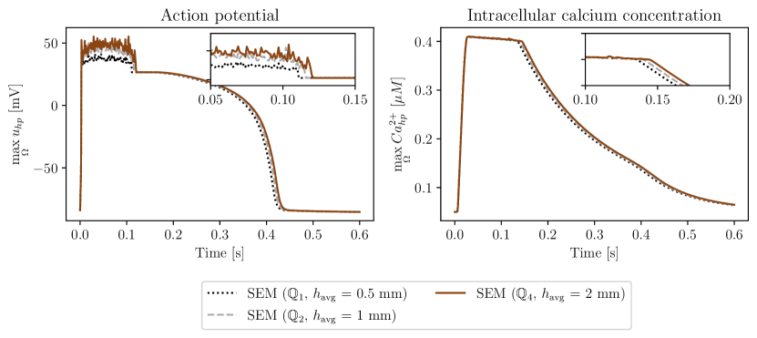
Figure 13: Zygote left ventricle. Minimum (top), average (mid), maximum (bottom) pointwise values of action potential $u$ and intracellular calcium concentration $Ca^{2+}$ over time, for ${\mathbb{Q}}_{1},{\mathbb{Q}}_{2},{\mathbb{Q}}_{4}$ elements and a fixed number of DOFs equal to $9^{\prime}116^{\prime}741$.

Mesh points number	Cells number	$h_{\mathrm{avg}}$ [$\mathrm{mm}$]	Local space	PCG iterations GMG preconditioner	Linear solver [$\mathrm{s}$]	Assemble rhs [$\mathrm{s}$]
$9^{\prime}116^{\prime}741$	$8^{\prime}939^{\prime}776$	0.05	$\mathbb{Q}_{1}$	2.54	12440.968	1241.884
$9^{\prime}116^{\prime}741$	$1^{\prime}117^{\prime}472$	0.1	$\mathbb{Q}_{2}$	2.54	12334.152	1020.451
$9^{\prime}116^{\prime}741$	$139^{\prime}684$	0.2	$\mathbb{Q}_{4}$	2.07	11328.664	687.311

Table 12: Zygote left ventricle. Computational times for ${\mathbb{Q}}_{1},{\mathbb{Q}}_{2},{\mathbb{Q}}_{4}$ elements and a fixed number of DOFs equal to $9^{\prime}116^{\prime}741$.

5.3 Whole–heart

The aim of this section is to show that our matrix–free solver can be successfully applied even in a much more complex framework. For this purpose we perform a numerical simulation in sinus rhythm with the Zygote four–chamber heart [41]. The settings of this test case can be found at the beginning of Section 5. We consider different ionic models, namely CRN [38] and TTP06 [37] for atria and ventricles, respectively. Furthermore, we model the valvular rings as non-conductive regions of the myocardium. The mesh is endowed with 355’664 cells and 10’355’058 nodes ($h_{\mathrm{avg}}=$1.6\text{\,}\mathrm{mm}$$). We employ the matrix–free solver and ${\mathbb{Q}}_{3}-$SEM, this choice is motivated by the numerical results obtained for the Niederer benchmark (Section 5.1) and the convergence test performed on the Zygote left ventricle geometry (Section 5.2).

We depict in Figure 14 the evolution of the transmembrane potential over time on the whole–heart geometry. The electric signal initiates at the sinoatrial node in the right atrium and then propagates to the left atrium and ventricles by means of preferential conduction lines, such as the Bachmann’s and His bundles [66]. The wavefront propagation appears very smooth, while accounting for small dissipation and dispersion throughout the heartbeat, as expected from the use of high–order discretizations [22].

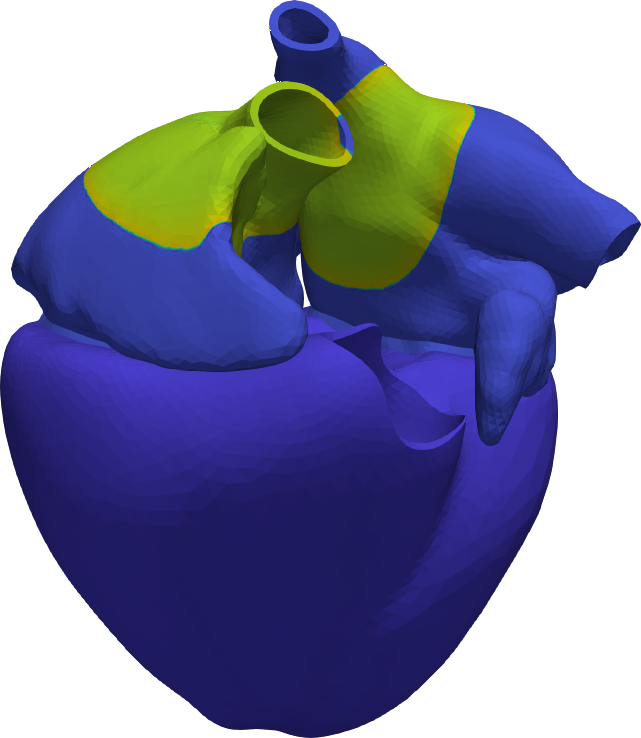
$t=$0.1\text{\,}\mathrm{s}$$

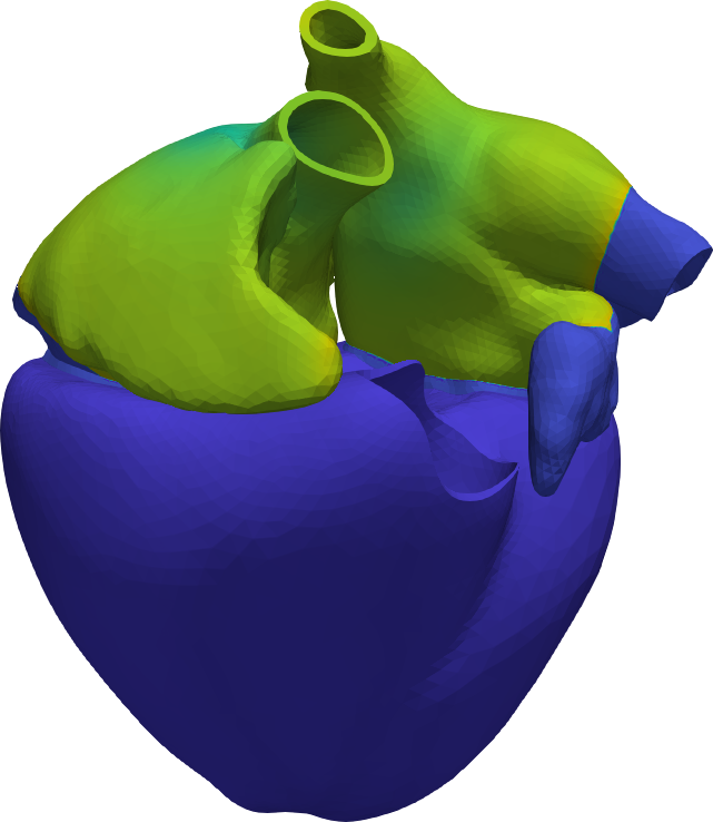
$t=$0.2\text{\,}\mathrm{s}$$

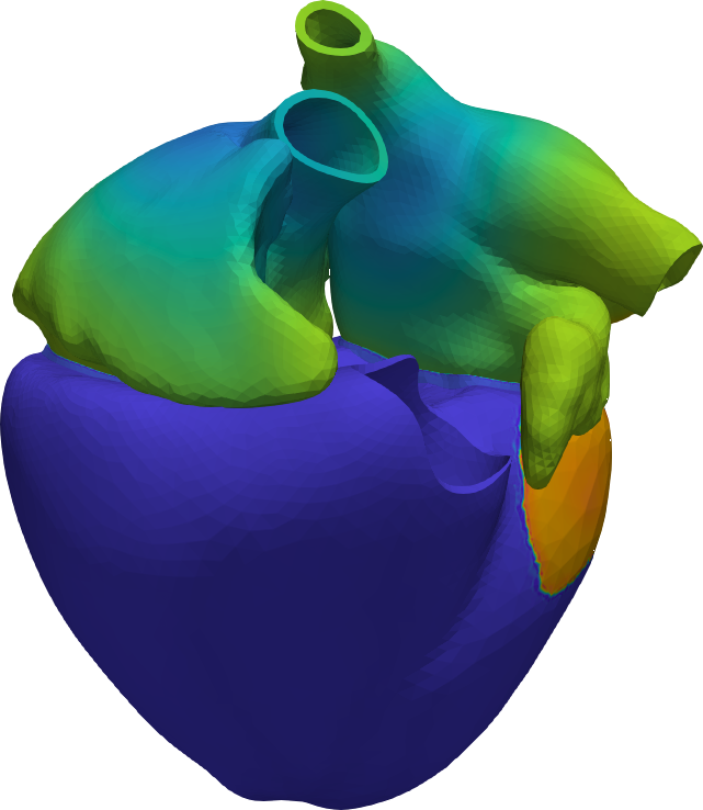
$t=$0.3\text{\,}\mathrm{s}$$

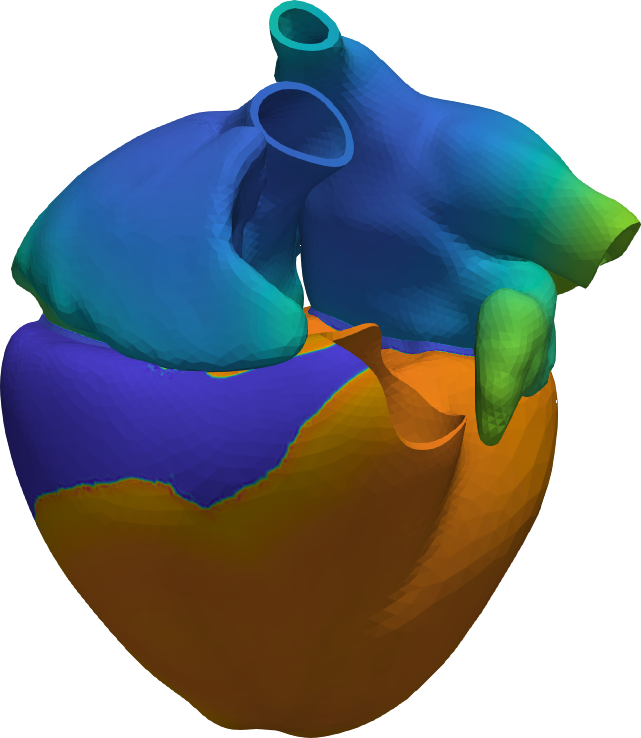
$t=$0.4\text{\,}\mathrm{s}$$

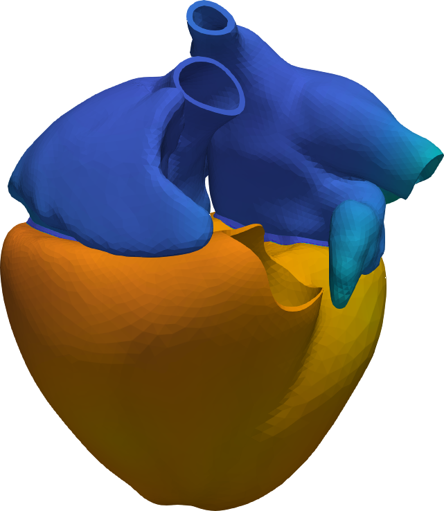
$t=$0.5\text{\,}\mathrm{s}$$

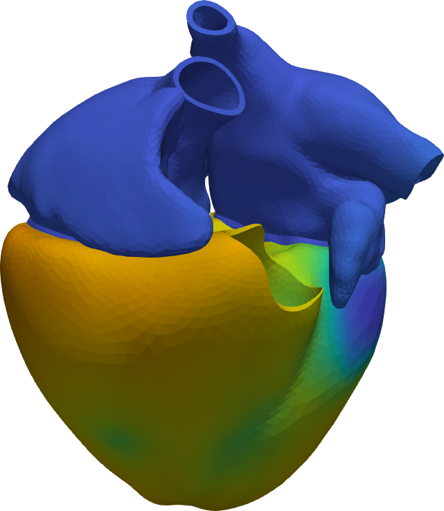
$t=$0.6\text{\,}\mathrm{s}$$

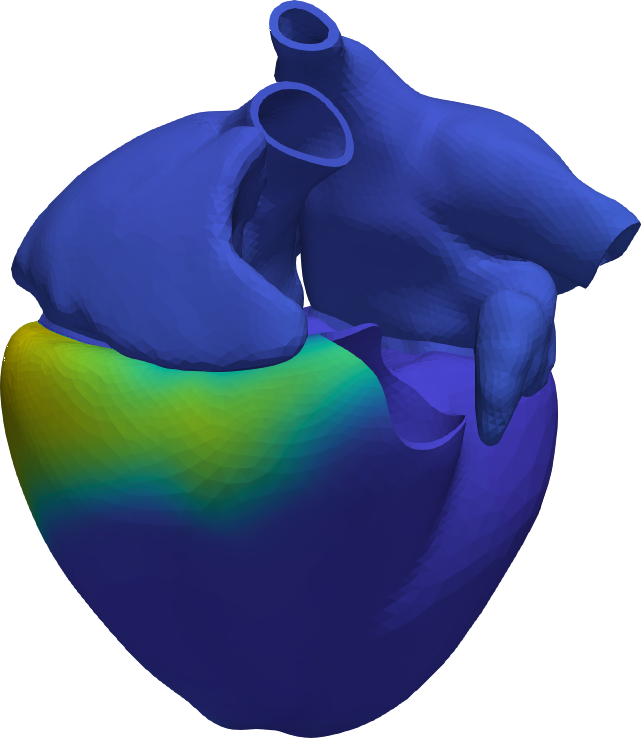
$t=$0.7\text{\,}\mathrm{s}$$

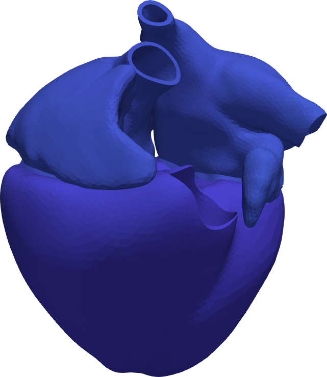
$t=$0.8\text{\,}\mathrm{s}$$

Figure 14: Zygote whole–heart. Time evolution of the transmembrane potential $u$ during one heartbeat.

6 Conclusions

We developed a matrix–free solver for cardiac electrophysiology tailored to the efficient use of high–order numerical methods. We employed the monodomain equation to model the propagation of the transmembrane potential and physiologically–based ionic models (CRN and TTP06) to describe the behaviour of different chemical species at the cell level.

We run several electrophysiological simulations for three different test cases, namely a slab of cardiac tissue, the Zygote left ventricle and the Zygote whole–heart to demonstrate the effectiveness and generality of our matrix–free solver in combination with Spectral Element Methods. SEM and SEM–NI provided comparable numerical results in terms of both accuracy and efficiency. Furthermore, we showed the importance of considering high–order Finite Elements in improving the accuracy and the computational burden for this class of mathematical problems, i.e. with sharp wavefronts involved.

Our matrix–free solver outperforms state–of–the–art matrix–based solvers in terms of computational costs and memory requirements. This is true even when matrix–vector products are computed without any matrix–free preconditioner, thanks to both vectorization and sum–factorization. Finally, the low memory footprint of the matrix–free implementation may allow for the development of GPU–based solvers of the cardiac function.

Appendix A

Let us consider the domain $\Omega\times(0,T)$ with $\Omega=(0,$1\text{\,}\mathrm{cm}$)^{2}$ and $T=$1\text{\,}\mathrm{s}$$. For the discretization we have taken a mesh size $h=$0.5\text{\,}\mathrm{mm}$$ (consistently with those chosen in the simulations shown in Section 5), polynomial degree $p=3$ and $p=4$, and the BDF schemes of order 1, 2, and 3 in time. Then we have measured the errors

$$\mathrm{err}_{H^{1}} =\left(\Delta t\sum_{n}\left\|u_{hp}(t_{n})-u(t^{n})\right\|^{2}_{H^{1}(\Omega)}\right)^{\frac{1}{2}},$$ (15a)

$$\mathrm{err}_{L^{2}} =\left(\Delta t\sum_{n}\left\|u_{hp}(t_{n})-u(t^{n})\right\|^{2}_{L^{2}(\Omega)}\right)^{\frac{1}{2}},$$ (15b)

between the exact solution $u$ and the fully discrete SEM–NI solution $u_{hp}$.

We have considered the exact solutions $u({\bf x},t)=(x_{1}^{2}+x_{2}^{2})(2+\sin(\pi t))$ and $u({\bf x},t)=\sin(\pi x_{1})\sin(\pi x_{2})(2+\sin(\pi t))$. The former one is solved exactly in space by both ${\mathbb{Q}}_{3}$ and ${\mathbb{Q}}_{4}$ discretizations, so that in Figure 15 we can appreciate the full convergence order in time of all the three schemes BDF1, BDF2, and BDF3. On the contrary, the latter solution is not captured exactly. The associated errors are shown in Figure 16 and we observe that they are bounded from below from the space discretization error when $\Delta t\lesssim 10^{-4}\,$\mathrm{s}$$, making the higher accuracy of BDF3 worthless. We notice that $\Delta t=10^{-4}\,$\mathrm{s}$$ coincides with the time step of $0.1\text{\,}\mathrm{ms}$ used in the simulations reported in Section 5. We remark that the numerical solutions we are looking for in cardiac electrophysiology typically feature steepest gradients than those we have considered in these examples, thus it is unlikely that the plateaux in the errors starts in correspondence of time steps much smaller than $10^{-4}\,$\mathrm{ms}$$. Finally, we bear in mind that, while BDF2 is absolutely stable, BDF3 is not, then special care should be given to the choice of the time step.

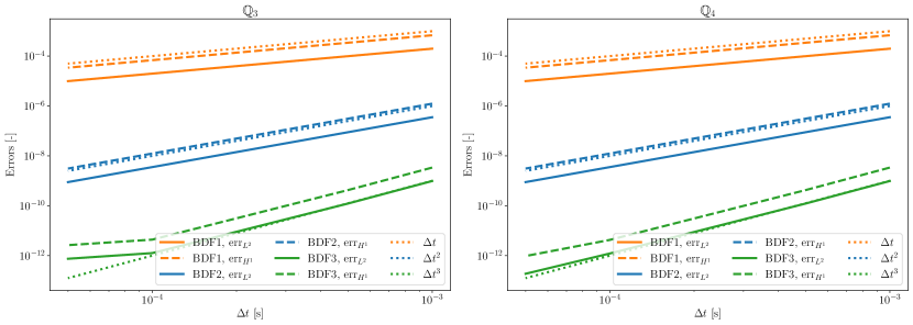
Figure 15: Errors (15) for SEM–NI discretization of the heat equation, with $h=0.5$mm and test solution $u({\bf x},t)=(x_{1}^{2}+x_{2}^{2})(2+\sin(\pi t))$. $p=3$ on the left and $p=4$ on the right

Figure 16: Errors (15) for SEM–NI discretization of the heat equation, with $h=0.5$mm and test solution $u({\bf x},t)=\sin(\pi x_{1})\sin(\pi x_{2})(2+\sin(\pi t))$. $p=3$ on the left and $p=4$ on the right

References

- [1] T. Gerach, S. Schuler, J. Fröhlich, L. Lindner, , E. Kovacheva, R. Moss, E. Wülfers, G. Seemann, C. Wieners, A. Loewe, Electro-Mechanical Whole-Heart Digital Twins: A Fully Coupled Multi-Physics Approach, Mathematics 9 (11).
- [2] R. Gray, P. Pathmanathan, Patient-Specific Cardiovascular Computational Modeling: Diversity of Personalization and Challenges, Journal of Cardiovascular Translational Research 11 (2018) 80–88.
- [3] R. Piersanti, F. Regazzoni, M. Salvador, A. Corno, L. Dede’, C. Vergara, A. Quarteroni, 3D-0D closed-loop model for the simulation of cardiac biventricular electromechanics, Computer Methods in Applied Mechanics and Engineering 391 (2022) 114607.
- [4] M. Potse, D. Krause, W. Kroon, R. Murzilli, S. Muzzarelli, F. Regoli, E. Caiani, F. Prinzen, R. Krause, A. Auricchio, Patient-specific modelling of cardiac electrophysiology in heart-failure patients, Europace 16 (2014) v56–iv61.
- [5] M. Strocchi, C. Augustin, M. Gsell, E. Karabelas, A. Neic, K. Gillette, O. Razeghi, A. Prassl, E. Vigmond, J. Behar, J. Gould, B. Sidhu, C. Rinaldi, M. Bishop, G. Plank, S. Niederer, A publicly available virtual cohort of four-chamber heart meshes for cardiac electro-mechanics simulations, PLOS ONE 15 (2020) 1–26.
- [6] A. Quarteroni, L. Dede’, A. Manzoni, C. Vergara, Mathematical Modelling of the Human Cardiovascular System: Data, Numerical Approximation, Clinical Applications, Cambridge University Press, 2019.
- [7] N. A. Trayanova, R. Winslow, Whole-Heart Modeling: Applications to Cardiac Electrophysiology and Electromechanics, Circulation Research 108 (1) (2011) 113–128.
- [8] P. Colli Franzone, L. Pavarino, S. Scacchi, Mathematical cardiac electrophysiology, Vol. 13, Springer, 2014.
- [9] H. Arevalo, F. Vadakkumpadan, E. Guallar, A. Jebb, P. Malamas, K. Wu, N. Trayanova, Arrhythmia risk stratification of patients after myocardial infarction using personalized heart models, Nature Communications 7 (2016) 11437.
- [10] J. Bayer, V. Sobota, A. Moreno, P. Jais, E. Vigmond, The Purkinje network plays a major role in low-energy ventricular defibrillation, Computers in Biology and Medicine 141 (2022) 105133.
- [11] K. Gillette, M. Gsell, A. Prassl, E. Karabelas, U. Reiter, G. Reiter, T. Grandits, C. Payer, D. Štern, M. Urschler, J. Bayer, C. Augustin, A. Neic, T. Pock, E. Vigmond, G. Plank, A Framework for the generation of digital twins of cardiac electrophysiology from clinical 12-leads ECGs, Medical Image Analysis 71 (2021) 102080.
- [12] C. Mendonca Costa, A. Neic, E. Kerfoot, B. Porter, B. Sieniewicz, J. Gould, B. Sidhu, Z. Chen, G. Plank, C. Rinaldi, M. Bishop, S. Niederer, Pacing in proximity to scar during cardiac resynchronization therapy increases local dispersion of repolarization and susceptibility to ventricular arrhythmogenesis, Heart Rhythm 16 (10) (2019) 1475–1483.
- [13] A. Quarteroni, A. Valli, Numerical Approximation of Partial Differential Equations, Springer Verlag, Heidelberg, 1994.
- [14] L. Woodworth, B. Cansız, M. Kaliske, A numerical study on the effects of spatial and temporal discretization in cardiac electrophysiology, International Journal for Numerical Methods in Biomedical Engineering 37 (5) (2021) e3443.
- [15] A. Patera, A spectral element method for fluid dynamics: laminar flow in a channel expansion, Journal of Computational Physics 54 (1984) 468–488.
- [16] Y. Maday, A. Patera, Spectral element methods for the incompressible Navier-Stokes equations, in: State-of-the-Art Surveys on Computational Mechanics, A.K. Noor and J. T. Oden, 1989, pp. 71–143.
- [17] C. Canuto, M. Hussaini, A. Quarteroni, T. Zang, Spectral Methods. Evolution to Complex Geometries and Applications to Fluid Dynamics, Springer, Heidelberg, 2007.
- [18] D. Arnold, F. Brezzi, B. Cockburn, L. Marini, Unified analysis of discontinuous Galerkin methods for elliptic problems, SIAM Journal on Numerical Analysis 39 (5) (2001) 1749–1779.
- [19] B. Cockburn, C.-W. Shu, The local discontinuous galerkin method for time-dependent convection-diffusion systems, SIAM Journal on Numerical Analysis 35 (6) (1998) 2440–2463.
- [20] R. LeVeque, Finite volume methods for hyperbolic problems, Cambridge Texts in Applied Mathematics, Cambridge University Press, Cambridge, 2002.
- [21] J. A. Cottrell, T. J. R. Hughes, Y. Bazilevs, Isogeometric Analysis: Toward Integration of CAD and FEA, Wiley, 2009.
- [22] M. Bucelli, M. Salvador, L. Dede’, A. Quarteroni, Multipatch Isogeometric Analysis for electrophysiology: Simulation in a human heart, Computer Methods in Applied Mechanics and Engineering 376 (2021) 113666.
- [23] C. Cantwell, S. Yakovlev, R. Kirby, N. Peters, S. Sherwin, High-order spectral/hp element discretisation for reaction–diffusion problems on surfaces: Application to cardiac electrophysiology, Journal of Computational Physics 257 (2014) 813–829.
- [24] Y. Coudière, R. Turpault, Very high order finite volume methods for cardiac electrophysiology, Computers & Mathematics with Applications 74 (4) (2017) 684–700.
- [25] J. Hoermann, C. Bertoglio, M. Kronbichler, M. Pfaller, R. Chabiniok, W. Wall, An adaptive hybridizable discontinuous Galerkin approach for cardiac electrophysiology, International Journal for Numerical Methods in Biomedical Engineering 34 (5).
- [26] K. Vincent, M. Gonzales, A. Gillette, C. Villongco, S. Pezzuto, J. Omens, M. Holst, A. McCulloch, High-order finite element methods for cardiac monodomain simulations, Frontiers in Physiology 6 (Aug).
- [27] D. Arndt, N. Fehn, G. Kanschat, K. Kormann, M. Kronbichler, P. Munch, W. Wall, J. Witte, ExaDG: High-Order Discontinuous Galerkin for the Exa-Scale, in: Software for Exascale Computing - SPPEXA 2016-2019, Springer International Publishing, Cham, 2020, pp. 189–224.
- [28] S. Orszag, Spectral methods for problem in complex geometries, Journal of Computational Physics 37 (1980) 70–92.
- [29] J. Melenk, K. Gerdes, C. Schwab, Fully discrete finite elements: Fast quadrature, Computer Methods in Applied Mechanics and Engineering 190 (32-33) (2001) 4339 – 4364.
- [30] M. Kronbichler, K. Kormann, A generic interface for parallel cell-based finite element operator application, Computers and Fluids 63 (2012) 135–147.
- [31] Y. Xia, K. Wang, H. Zhang, Parallel Optimization of 3D Cardiac Electrophysiological Model Using GPU, Computational and Mathematical Methods in Medicine 2015 (2015) 862735.
- [32] M. Kronbichler, K. Ljungkvist, Multigrid for Matrix-Free High-Order Finite Element Computations on Graphics Processors, ACM Transactions on Parallel Computing 6 (1) (2019) 1–32.
- [33] G. Del Corso, R. Verzicco, F. Viola, A fast computational model for the electrophysiology of the whole human heart, Journal of Computational Physics 457 (2022) 111084.
- [34] S. A. Niederer, E. Kerfoot, A. P. Benson, M. O. Bernabeu, O. Bernus, C. Bradley, E. M. Cherry, R. Clayton, F. H. Fenton, A. Garny, E. Heidenreich, S. Land, M. Maleckar, P. Pathmanathan, G. Plank, J. F. Rodríguez, I. Roy, F. B. Sachse, G. Seemann, O. Skavhaug, N. Smith, Verification of cardiac tissue electrophysiology simulators using an N-version benchmark, Philosophical Transactions of the Royal Society A: Mathematical, Physical and Engineering Sciences 369 (1954) (2011) 4331–51.
- [35] P. C. Africa, lifex: a flexible, high performance library for the numerical solution of complex finite element problems, SoftwareX 20 (2022) 101252. doi:10.1016/j.softx.2022.101252.
- [36] D. Arndt, W. Bangerth, B. Blais, T. Clevenger, M. Fehling, A. Grayver, T. Heister, L. Heltai, M. Kronbichler, M. Maier, P. Munch, J. Pelteret, R. Rastak, I. Tomas, B. Turcksin, Z. Wang, D. Wells, The deal.II library, Version 9.2, Journal of Numerical Mathematics 28 (3) (2020) 131–146.
- [37] K. ten Tusscher, A. Panfilov, Alternans and spiral breakup in a human ventricular tissue model, American Journal of Physiology Heart and Circulation Physiology 291 (2006) 1088–1100.
- [38] M. Courtemanche, R. Ramirez, S. Nattel, Ionic mechanisms underlying human atrial action potential properties: insights from a mathematical model, American Journal of Physiology Heart and Circulation Physiology 275 (1) (1998) H301–H321.
- [39] R. Piersanti, P. Africa, M. Fedele, C. Vergara, L. Dede’, A. Corno, A. Quarteroni, Modeling cardiac muscle fibers in ventricular and atrial electrophysiology simulations, Computer Methods in Applied Mechanics and Engineering 373 (2021) 113468.
- [40] P. Africa, R. Piersanti, M. Fedele, L. Dede’, A. Quarteroni, An open tool based on lifex for myofibers generation in cardiac computational models (2022). doi:10.48550/arXiv.2201.03303.
- [41] Zygote Media Group Inc., Zygote Solid 3D heart Generation II, Development Report (2014).
- [42] C. Bernardi, Y. Maday, Spectral, spectral element and mortar element methods, in: Theory and numerics of differential equations (Durham, 2000), Universitext, Springer, Berlin, 2001, pp. 1–57.
- [43] G. Karniadakis, S. Sherwin, Spectral/hp Element Methods for Computational Fluid Dynamics, Oxford University Press, 2005, 2nd ed.
- [44] C. Canuto, M. Hussaini, A. Quarteroni, T. Zang, Spectral Methods. Fundamentals in Single Domains, Springer, Heidelberg, 2006.
- [45] P. Gervasio, L. Dede’, O. Chanon, A. Quarteroni, A computational comparison between isogeometric analysis and spectral element methods: accuracy and spectral properties, J. Sci. Comput. 83 (18). doi:10.1007/s10915-020-01204-1.
- [46] B. Szabó, I. Babuška, Finite Element Analysis, John Wiley & sons, New York, 1991.
- [47] C. Schwab, and finite element methods, Oxford University Press, Oxford, 1998.
- [48] N. Fehn, W. Wall, M. Kronbichler, A matrix-free high-order discontinuous Galerkin compressible Navier-Stokes solver: A performance comparison of compressible and incompressible formulations for turbulent incompressible flows, International Journal for Numerical Methods in Fluids 89 (3) (2019) 71–102.
- [49] F. Regazzoni, M. Salvador, P. Africa, M. Fedele, L. Dede’, A. Quarteroni, A cardiac electromechanical model coupled with a lumped-parameter model for closed-loop blood circulation, Journal of Computational Physics 457 (2022) 111083.
- [50] A. Quarteroni, T. Lassila, S. Rossi, R. Ruiz-Baier, Integrated Heart-Coupling multiscale and multiphysics models for the simulation of the cardiac function, Computer Methods in Applied Mechanics and Engineering 314 (2017) 345–407.
- [51] P. Gervasio, F. Saleri, A. Veneziani, Algebraic fractional step schemes with spectral methods for the incompressible Navier-Stokes equations, Journal of Computational Physics 214 (1) (2006) 347–365.
- [52] J. M. Cebrian, L. Natvig, M. Jahre, Scalability analysis of AVX-512 extensions, The Journal of Supercomputing 76 (3) (2020) 2082–2097.
- [53] D. Zhong, Q. Cao, G. Bosilca, J. Dongarra, Using long vector extensions for MPI reductions, Parallel Computing 109 (2022) 102871.
-
[54]
Message Passing Interface Forum,
MPI: A
Message-Passing Interface Standard Version 4.0 (Jun. 2021).
URL https://www.mpi-forum.org/docs/mpi-4.0/mpi40-report.pdf - [55] M. Kronbichler, K. Kormann, Fast matrix-free evaluation of discontinuous Galerkin finite element operators, ACM Transactions on Mathematical Software 45 (3) (2019) 1–40.
- [56] C. Cantwell, S. Sherwin, R. Kirby, P. Kelly, From h to p efficiently: Strategy selection for operator evaluation on hexahedral and tetrahedral elements, Computers and Fluids 43 (1) (2011) 23 – 28.
- [57] B. Janssen, G. Kanschat, Adaptive Multilevel Methods with Local Smoothing for and Conforming High Order Finite Element Methods, SIAM Journal on Scientific Computing 33 (4) (2011) 2095–2114.
- [58] J. Xu, L. Zikatanov, Algebraic multigrid methods, Acta Numerica 26 (2017) 591 – 721.
- [59] P. Bastian, E. Müller, S. Müthing, M. Piatkowski, Matrix-free multigrid block-preconditioners for higher order discontinuous Galerkin discretisations, J. Comput. Phys. 394 (2019) 417–439. doi:10.1016/j.jcp.2019.06.001.
- [60] N. Fehn, P. Munch, W. Wall, M. Kronbichler, Hybrid multigrid methods for high-order discontinuous Galerkin discretizations, J. Comput. Phys. 415 (2020) 109538. doi:10.1016/j.jcp.2020.109538.
- [61] H. Sundar, G. Stadler, G. Biros, Comparison of multigrid algorithms for high-order continuous finite element discretizations, Numerical Linear Algebra with Applications 22.
- [62] U. Trottenberg, C. Oosterlee, A. Schüller, Multigrid, Elsevier Academic Press, London, UK, 2001.
- [63] T. Clevenger, T. Heister, G. Kanschat, M. Kronbichler, A Flexible, Parallel, Adaptive Geometric Multigrid Method for FEM, ACM Transactions on Mathematical Software 47 (1).
- [64] M. Adams, M. Brezina, J. Hu, R. Tuminaro, Parallel multigrid smoothing: Polynomial versus Gauss-Seidel, Journal of Computational Physics 188 (2) (2003) 593 – 610.
- [65] M. Gee, C. Siefert, J. Hu, R. Tuminaro, M. Sala, ML 5.0 Smoothed Aggregation User’s Guide (SAND2006-2649).
- [66] R. Harrington, J. Narula, Z. Eapen, Hurst’s the Heart, MacGraw-Hill, 2011.