Precision boson-jet azimuthal decorrelation at hadron colliders

Abstract

The azimuthal angular decorrelation of a vector boson and jet is sensitive to QCD radiation, and can be used to probe the quark-gluon plasma in heavy-ion collisions. By using a recoil-free jet definition, the sensitivity to contamination from soft radiation on the measurement is reduced, and the complication of non-global logarithms is eliminated from our theoretical calculation. Specifically we will consider the $p_{T}^{n}$ recombination scheme, as well as the $n\to\infty$ limit, known as the winner-take-all scheme. These jet definitions also significantly simplify the calculation for a track-based measurement, which is preferred due to its superior angular resolution. We present a detailed discussion of the factorization in Soft-Collinear Effective Theory, revealing why the transverse momentum $\vec{q}_{T}$ is more complicated than the azimuthal angle. We show that potential glauber contributions do not spoil our factorization formalism, at least up to and including order $\alpha_{s}^{3}$. The resummation is carried out using the renormalization group, and all necessary ingredients are collected or calculated. We conclude with a detailed phenomenological study, finding an enhanced matching correction for high jet $p_{T}$ due to the electroweak collinear enhancement of a boson emission off di-jets. We also compare with the Pythia event generator, finding that our observable is very robust to hadronization and the underlying event.

1 Introduction

At hadron colliders, the simplest jet measurements involve a single jet, which recoils against a color-singlet object produced alongside it. In the transverse plane momentum conservation enforces an (almost) back-to-back orientation of the jet and the color singlet. We will focus on the case of a $Z$ boson balancing against the jet, but our approach can also be applied to other color singlets such as a photon, $W$ or Higgs boson. With only a single jet in the final state, this process is the minimal extension beyond the 0-jet case at hadron colliders, and of significant experimental interest at hadron colliders Chatrchyan:2013tna ; CMS:2013myp ; ATLAS:2016jxf ; Khachatryan:2016crw ; Sirunyan:2017jic ; Aaboud:2017kff ; CMS:2017ehl . In particular, in heavy-ion collisions Sirunyan:2017jic ; CMS:2017ehl the boson provides an inert reference for the jet since it does not interact strongly with the quark-gluon plasma Kartvelishvili:1995fr . Therefore the process can be used to study the medium properties.

Accordingly, efforts towards precise theoretical predictions for boson-jet correlations have been made in hadron collisions: Fixed-order results have been calculated to next-to-next-to-leading order in the QCD corrections Chen:2014gva ; Ridder:2015dxa ; Boughezal:2015dva ; Boughezal:2015ded ; Boughezal:2015dra ; Boughezal:2015aha ; Campbell:2016lzl ; Gehrmann-DeRidder:2017mvr ; Chen:2019zmr ; Gehrmann-DeRidder:2019avi ; Czakon:2020coa ; Mondini:2021nck ; Gauld:2021pkr , while resummed results for the near-planar case exhibiting Sudakov logarithms have been derived to next-to-leading logarithmic (NLL) accuracy at hadron colliders for various vector (and scalar) bosons Banfi:2008qs ; Chen:2018fqu ; Sun:2018icb ; Chien:2019gyf ; Buonocore:2021akg ; Hatta:2021jcd . Efforts have also been made in heavy-ion collisions to study the azimuthal decorrelation Chen:2018fqu as well as the transverse momentum imbalance and other related observables (see Cao:2020wlm for a review).

In this paper, we study the deviation from the back-to-back configuration in $V$+jet production, by including QCD corrections from the dominant contribution from soft and collinear radiation. We demonstrate in detail that the azimuthal decorrelation, in combination with a recoil-free jet definition, has a particularly simple theoretical description: the non-global logarithms (NGLs) Dasgupta:2001sh are absent. This allows us to obtain resummed predictions at next-to-next-to-leading logarithmic (NNLL) accuracy, as first reported in Chien:2020hzh , and opens up the possibility for an N³LL analysis to match to the next-to-next-to-leading order (NNLO) calculations in Chen:2014gva ; Ridder:2015dxa ; Boughezal:2015dva ; Boughezal:2015ded ; Boughezal:2015dra ; Boughezal:2015aha ; Campbell:2016lzl ; Gehrmann-DeRidder:2017mvr ; Chen:2019zmr ; Gehrmann-DeRidder:2019avi ; Czakon:2020coa ; Mondini:2021nck ; Gauld:2021pkr , since many ingredients are already available. Also, if the jet is measured using charged particle tracks, rather than the full set of all final state particles, this can be described using the track function formalism Chang:2013rca ; Chang:2013iba with minimal nonperturbative input (an integral over the track functions). In contrast, the azimuthal decorrelation with the standard jet axis suffers — as is typical for jet observables — from the presence of non-global logarithms, which has so far hindered resummation beyond the NLL accuracy. The effects of NGLs are instead power suppressed in the case we consider. While our main focus is on the Winner-Take-All (WTA) recombination scheme Salam:WTAUnpublished ; Bertolini:2013iqa , we also determine the effect of a different choice of recoil-free (i.e. momentum-weighted) axis. This only leads to a minor modification in the constant term in the jet function. We furthermore explore the other component of the $V$+jet transverse momentum imbalance, which we refer to as the radial decorrelation. Because the factorization structure is much more complicated, even for a recoil-free axis, we do not further pursue it here, but include it as an illustrative foil to the azimuthal decorrelation.

The program outlined in the previous paragraph is conducted based on a factorization formula derived using Soft-Collinear Effective Theory (SCET) Bauer:2000yr ; Bauer:2001ct ; Bauer:2001yt ; Bauer:2002nz ; Beneke:2002ph . We calculate the necessary ingredient functions, where not yet available, and explore potentially factorization violating effects from Glauber gluons, identifying the order at which they may first contribute.

Our main result consists of a phenomenological study, consisting of numerical results for the analytic resummation at NNLL accuracy. We include a discussion of the resummation, perturbative uncertainties, nonperturbative effects, and the matching to fixed order. We furthermore study features of this observable using Pythia, and compare to our NNLL result. As promised by the recoil-free axis, we find that the observable is insensitive to soft effects (hadronization, underlying event), a rather small sensitivity to the jet radius, and negligible differences when measuring the decorrelation on tracks. The uncertainty band of our resummed predictions are reduced when going from NLL to NNLL. Our resummed results are consistent with Pythia, except for the matching corrections from the NLO cross section (as we didn’t match Pythia to NLO). These matching corrections are substantial for high jet $p_{T}$, and arise from the boson being emitted from a leading order dijet configuration. Though this is formally power suppressed in the back-to-back limit, it is enhanced by an electroweak logarithm. While we focus on the WTA axis, we also explore $p_{T}^{n}$-weighted recombination schemes, and these conclusions also hold there (if $n>1$).

The paper is structured as follows: We introduce the kinematic setup and discuss different observables measuring the transverse momentum decorrelation of the $V+$jet pair in section 2. Section 3 establishes the factorization formula, gathers the available ingredient functions, and includes a brief discussion of factorization violation induced by a Glauber mode. Section 4 contains various calculations relating to the jet function: The linearly polarized jet function appearing in our factorization formula, as well as the changes to the jet function induced by the use of a different recoil-free jet axis or track-based measurements, respectively. We establish our resummation strategy in section 5 (with certain ingredients relegated to appendix A) which is then carried out to derive the results in section 6. We conclude in section 7.

2 Boson-jet correlation

2.1 Geometry of the collision

We begin by describing the geometry of the collision and defining the observable for which we perform the resummation. It will be instructive to contrast our target observable, the azimuthal decorrelation, with the closely related radial decorrelation. (These correspond to the two components of the difference in transverse momentum between vector boson and jet.) This comparison will demonstrate in detail where simplifications due to the choice of a recoil-free recombination scheme arise and how non-global effects are suppressed: While using a recoil-free axis removes non-global logarithms for the azimuthal decorrelation, the radial variety still suffers from NGLs and needs to include effects related to the technical definition of this axis. For concreteness we discuss the case of the Winner-Take-All (WTA) axis.

Figure 1: Left: The azimuthal angle between the vector boson (green) and jet axis (blue) is related to the momentum of the vector boson $p_{x,V}$ transverse to the colliding protons (red) and jet. Collinear initial (purple) and final-state (blue) radiation and soft radiation (magenta) is also shown. Right: Schematic of the transverse plane: the angle $\phi_{c}$ between WTA axis (along $y$ axis) and collective collinear momentum, the angle $\phi_{ij}$ between two generic collinear emissions $i$ and $j$, and the angular decorrelation observable $\delta\phi$. These quantities are of the same parametric size.

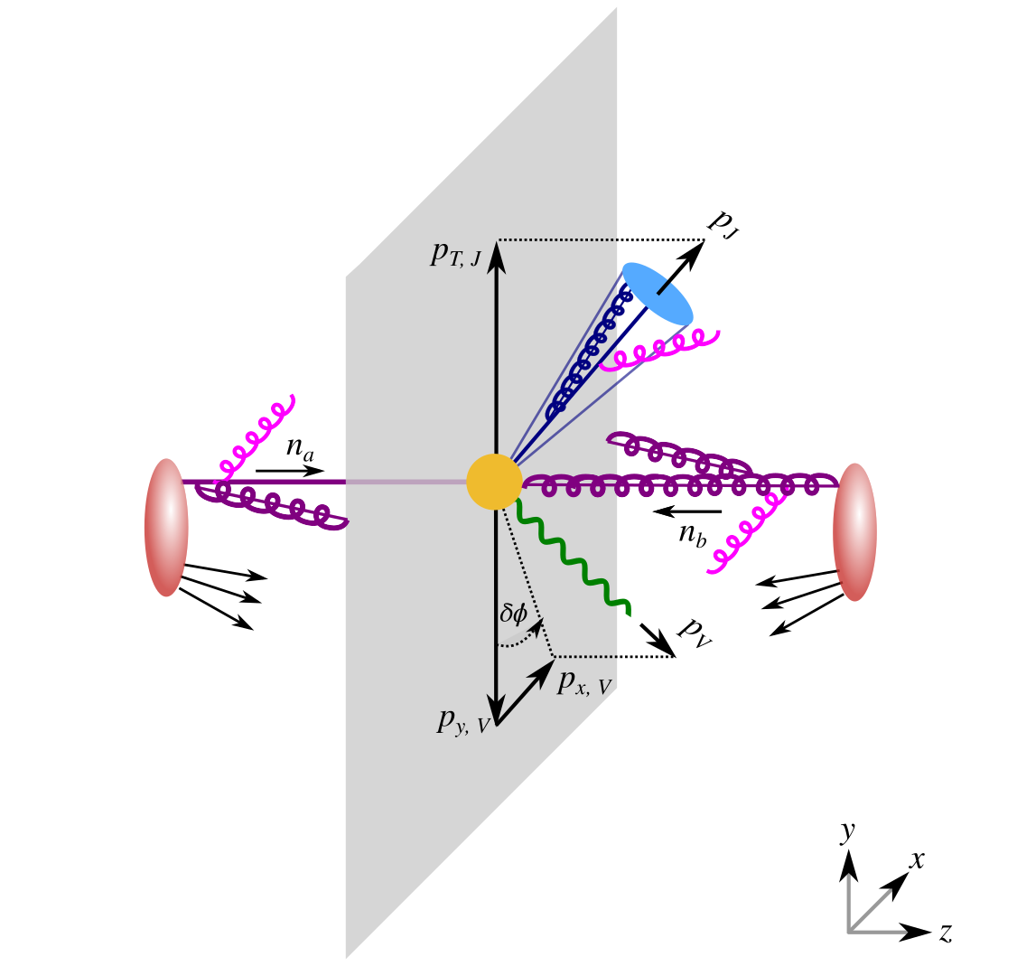
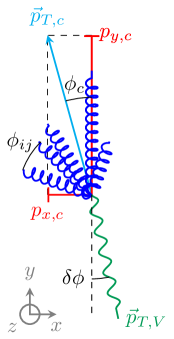
The geometric setup is illustrated in the left panel of figure 1, where we choose to align the $y$-axis with the reconstructed jet axis (its projection onto the transverse plane, to be precise). Our starting point is momentum conservation in the transverse plane, which reads

$$\vec{p}_{T,a}+\vec{p}_{T,b}+\vec{p}_{T,S}+\vec{p}_{T,c}+\vec{p}_{T,V}=0,$$ (1)

and expresses that the vector boson (with transverse momentum $\vec{p}_{T,V}$) recoils against emissions off the beams ($\vec{p}_{T,a},\vec{p}_{T,b}$), soft radiation ($\vec{p}_{T,S}$), and the total collinear radiation in the jet ($\vec{p}_{T,c}$). Note that $\vec{p}_{T,c}$ is non-trivial, i.e. possesses both $x$ and $y$-components, as we chose to align our coordinate axes with the reconstructed jet axis $\vec{p}_{T,J}$, which in the WTA case does not follow the collective momentum of all collinear emissions in the jet: As detailed in ref. Bertolini:2013iqa , the WTA axis always follows the orientation of one input particle (not necessarily the most energetic one, which would not be collinear safe), whereas the total momentum in general is not aligned with any individual particle direction.

To illustrate this point, we revisit the WTA recombination scheme and the associated axis in detail: in sequential jet clustering algorithms, particles are pairwise recombined and assigned a joint 4-momentum. For the WTA recombination scheme, this joint momentum is taken massless, and points along the direction of the “harder” of the two particles in the pair. The criterion to determine which of two particles is the harder is typically the hierarchy in either the particle energy (“WTA-$E$-scheme”) or the transverse momentum (“WTA-$p_{T}$-scheme”). The latter choice is of course more suitable for hadron colliders and shall therefore be used here. The magnitude of the newly combined pseudo-particle is the sum of the energies or the scalar sum of transverse momenta — the “winner” absorbs the loser, so to speak. The WTA axis is then simply the final pseudo-particle after clustering. It is in principle possible that many soft emissions are clustered into one highly energetic pseudo particle that emerges as the winner, but this is extremely unlikely because they would have to be clustered together first to stand a chance against collinear emissions, contrary to the expectation that they are spread out over the jet. Thus the WTA axis will be aligned with one of the collinear emissions, rendering its direction free of soft recoil.

The WTA axis is a particularly powerful tool when combined with SCET, because it can exploit the parametric hierarchy of the modes in SCET to simplify the calculation: As stated, the magnitude of the jet axis will be a sum of transverse momenta

$$|\vec{p}_{T,J}|=\sum_{i}|\vec{p}_{T,i}|,$$ (2)

where the sum runs over all emissions in the jet. One consequence of the WTA recombination is then that soft emissions inside the jet can affect the magnitude as participants in this sum, but never the orientation, as soft emissions always lose against collinear emissions when determining with which emission the axis should be aligned. The dependence of the axis on soft emissions can be expanded away and represents a subleading effect in the effective theory — and in some cases even the dependence in the magnitude can be expanded away, with more details laid out in the following two sections.

The azimuthal angle is now directly related to the (dimensionful) offset between vector boson and reconstructed jet momentum, defined as

$$\vec{q}_{T} \equiv\vec{p}_{T,V}+\vec{p}_{T,J}$$

$$=\vec{p}_{T,J}-\vec{p}_{T,c}-\vec{p}_{T,a}-\vec{p}_{T,b}-\vec{p}_{T,S}.$$ (3)

In the absence of QCD radiation, $\vec{q}_{T}$ vanishes, and the limit of small $\vec{q}_{T}$ is of interest for the resummation. The angular decorrelation can be e.g. written as $\delta\phi=\arcsin q_{x}/|p_{T,V}|\approx q_{x}/|p_{T,V}|$, and is essentially a dimensionless version of the dimensionful $\vec{q}_{T}$.

2.2 Azimuthal and radial decorrelation

Besides the azimuthal decorrelation, which represents the tangential offset $q_{x}$ as shown in figure 1, we can define a second quantity of interest here, the radial decorrelation, using $q_{y}$. Using eq. (1) these can be written as

$$q_{x} =p_{x,V}+p_{x,J} q_{y} =p_{y,V}+p_{y,J}$$ (4)

$$=p_{x,V} =p_{y,J}-p_{y,a}-p_{y,b}-p_{y,S}-p_{y,c}$$

$$=-p_{x,a}-p_{x,b}-p_{x,S}-p_{x,c}$$

where we used that $p_{x,J}=0$ due to the alignment of the $y$-axis with the the WTA axis. We expect the contributions from the beams to be isotropic in the transverse plane (and their $x$- or $y$-dependence therefore to be similar) and the soft function to capture the $y$-dependence via its dependence on the geometry of the beam-jet system, so to proceed we need to understand the relation between $\vec{p}_{T,J}$ and $\vec{p}_{T,c}$, i.e. the reconstructed WTA axis and the collective collinear momentum of the jet, and their components. Right from the start it is clear that the radial decorrelation is more complex, as it involves a large cancellation between the boson and jet axis magnitude.

For $\vec{p}_{T,c}$ and its decomposition into $x$- and $y$-components, this yields the situation illustrated in the right panel in figure 1. Thus

$$p_{x,c}=|\vec{p}_{T,c}|\cdot\sin\phi_{c}\approx|\vec{p}_{T,c}|\cdot\phi_{c},$$ (5)

where $\vec{p}_{T,c}$ (which is of the order of the center-of-mass energy $Q$) is the vector sum of all collinear emissions off the parton initiating the jet, and $\phi_{c}$ measures the angular separation between the WTA axis and the collective collinear momentum flow.

To obtain $\delta\phi$ or $q_{x}$, we still need to include the collinear and soft contributions in eq. (4). As the $x$-direction is perpendicular to the plane containing both the jet and the beams, we expect the appropriate SCET modes to scale — with notation $p^{\mu}=(n_{b}\cdot p,n_{a}\cdot p,p_{\perp})$ — as

$$\begin{aligned} p_{a}&\sim Q(1,\phi_{c}^{2},\phi_{c}),\qquad\qquad&p_{b}&\sim Q(\phi_{c}^{2},1,\phi_{c}),\\ p_{S}&\sim Q(\phi_{c},\phi_{c},\phi_{c}),&p_{c}&\sim Q(1,\phi_{c}^{2},\phi_{c})_{J},\end{aligned}$$ (6)

where the scaling for the jet — with subscript $J$ — is to be understood as scaling of lightcone components based on the jet direction, i.e. $p^{\mu}=(\bar{n}_{J}\cdot p,n_{J}\cdot p,p_{\perp})_{J}$. We thus find a SCET_II situation, as expected for a de facto transverse momentum measurement.

Finally, note that there is no special dependence on soft in-jet radiation: It is always expanded away when the jet axis direction is determined, but it can also be expanded away in the magnitude in this case, as the azimuthal decorrelation only depends on the direction of the jet axis, which determines the coordinate system we use to define it.

2.3 Properties of the radial decorrelation

We will now contrast this surprisingly simple observable with the radial decorrelation $q_{y}$, where the details of the recombination become explicitly relevant. We emphasize that we do not wish to actually perform the resummation for this observable, but merely include this discussion to highlight why the azimuthal decorrelation is so amenable to precision calculations.

A key insight is that while $p_{y,J}$ in eq. (4) includes a sum over collinear (and soft) momenta, it makes use of a scalar sum and aligns it with a collinear emission’s direction, while $p_{y,c}$ is a component of a vector sum. Iterating the law of cosines/binomial theorem over all relevant momenta, the vector and scalar sum of collinear momenta can be related, to

$$\begin{aligned} |\vec{p}_{T,c}|=\biggl{|}\sum_{i\in c}\vec{p}_{T,i}\biggr{|}&=\sum_{i\in c}|\vec{p}_{T,i}|\cdot\sqrt{1-\frac{2\sum_{i<j}|\vec{p}_{T,i}||\vec{p}_{T,j}|(1-\cos\phi_{ij})}{(\sum_{i\in c}|\vec{p}_{T,i}|)^{2}}}.\end{aligned}$$ (7)

Here $\phi_{ij}$ are the pairwise opening angles between emissions $i$ and $j$, which satisfy $\phi_{ij}\ll 1$ because $i$ and $j$ are both collinear. Thus we can expand the above expression to obtain

$$\begin{aligned} \biggl{|}\sum_{i\in c}\vec{p}_{T,i}\biggr{|}&\approx\sum_{i\in c}|\vec{p}_{T,i}|-\frac{\sum_{i<j}|\vec{p}_{T,i}||\vec{p}_{T,j}|\phi^{2}_{ij}}{2\sum_{i\in c}|\vec{p}_{T,i}|}.\end{aligned}$$ (8)

We can now derive the expression for the radial decorrelation: As $p_{x,J}=0$ due to our choice of conventions, $p_{y,J}$ is the scalar sum of all momenta inside the jet, which for $R\gg\delta\phi$ includes all collinear radiation, as well as the soft emissions that end up in the jet: $p_{y,J}=|\vec{p}_{T,J}|=\sum_{i\in(s\in J)}|\vec{p}_{T,i}|+\sum_{i\in c}|\vec{p}_{T,i}|$. This leads to

$$\begin{aligned} q_{y}&=p_{y,J}-|\vec{p}_{T,c}|\cos\phi_{c}-p_{y,S}-p_{y,a}-p_{y,b}\\ &=\underbrace{-p_{y,a}-p_{y,b}}_{\text{beam functions}}+\underbrace{\sum_{i\in(s\in J)}|p_{T,i}|-p_{y,S}}_{\text{soft function}}+\underbrace{\sum_{i\in c}|\vec{p}_{T,i}|\frac{\phi_{c}^{2}}{2}+\frac{\sum_{(i<j)\in c}|\vec{p}_{T,i}||\vec{p}_{T,j}|\phi^{2}_{ij}}{2\sum_{i\in c}|\vec{p}_{T,i}|}}_{\text{jet function}},\end{aligned}$$ (9)

where the leading scalar sum of collinear momenta cancelled, and the corresponding functions in the factorization are indicated. The expected power counting of the modes involved is also non-trivial: The jet power counting is determined by its $\perp$-component, which must scale as $\mathcal{O}(Q\phi_{c})$, as the angle between WTA axis (i.e. one of the emissions) and the collective collinear momentum has to be parametrically similar to the opening angle of collinear splittings. The transverse components $p_{y,a}$ and $p_{y,b}$ for the beams must scale as $\mathcal{O}(Q\phi_{c}^{2})$ to contribute at equal footing with the jet contributions in (9). The soft contributions are isotropic and a similar argument applies. It thus follows that

$$\begin{aligned} p_{a}&\sim Q(1,\phi_{c}^{4},\phi_{c}^{2}),\qquad\qquad&p_{b}&\sim Q(\phi_{c}^{4},1,\phi_{c}^{2}),\\ p_{S}&\sim Q(\phi_{c}^{2},\phi_{c}^{2},\phi_{c}^{2}),&p_{J}&\sim Q(1,\phi_{c}^{2},\phi_{c})_{J},\end{aligned}$$ (10)

which is an interesting combination of SCET_I and SCET_II characteristics. For the beams this is a transverse momentum measurement, and so they share the virtuality of the soft emissions, as typical in SCET_II. The jet, however, measures essentially an invariant-mass-like observable, a SCET_I situation.

We also note that the differing treatment of soft radiation inside and outside the jet means this observable exhibits non-global logarithms. This is a persistent feature: while it is e.g. possible to remove the term depending on pairs of collinear emissions from eq. (9) by determining the magnitude of $\vec{p}_{T,J}$ using a vector-sum-based recombination scheme, the inclusion of soft in-jet emissions will also be present in such a case.

From the above discussion we can now understand why the azimuthal decorrelation is so simple, by comparison: The non-trivial effects present in its radial sibling, including the appearance of non-global logarithms, are $\mathcal{O}(\phi_{c}^{2})$ effects, and are therefore power suppressed compared to the dominant contributions to azimuthal decorrelation in (5), which are $\mathcal{O}(\phi_{c})$.

2.4 Extensions

We conclude this section, by discussing other recoil-free axes, double differential measurements in the azimuthal and radial decorrelation and tracks for the radial decorrelation:

First, we note that the choice of a recoil-free axis other than the WTA-axis (in essence the FastJet Cacciari:2011ma recombination scheme of equation (4) with $w_{i}=p_{Ti}^{n}$ and $1<n<\infty$, see also eq. (4.2)) constitutes a small change for the azimuthal recombination: as long as it is recoil free, only the jet function will be changed, and we will calculate the corresponding jet function in sec. 4.2. (For the radial decorrelation this may be a more intricate affair, as subleading effects are elevated by virtue of a large cancellation.)

Second, we point out that measuring any quantity in the $\vec{q}$-plane other than the elementary $q_{x}$ and $q_{y}$ is a de facto double-differential measurement, and requires the specification of the relative scaling of the $q_{x}$ and $q_{y}$ components, to cleanly establish which contributions to the observable from the different regions (or ingredient functions) are subleading and can be neglected. This ultimately is a consequence of the different scaling of $q_{x}$ and $q_{y}$ themselves, in terms of power counting. In particular, one could consider $q_{x}\sim q_{y}$ or $q_{x}^{2}\sim Qq_{y}$, which correspond to making the factorization of the azimuthal or radial decorrelation differential in both $q_{x}$ and $q_{y}$, or something in between (see e.g. ref. Procura:2014cba for a factorization description of double differential measurements).

Finally, we point out that using track-based measurements is a possibility for the azimuthal decorrelation, and will be discussed in 4.3, but is firmly ruled out for the radial decorrelation. The reason is simply that the vector boson will always be fully reconstructed with all of its transverse momentum, but the jet axis is only established based on the particles included in the jet recombination. If all collinear particles are clustered into the jet, the jet axis magnitude is roughly equal to the total collinear transverse momentum, and the cancellation against the vector boson transverse momentum establishes the radial decorrelation as a small quantity, which vanishes in the singular limit. A resummation program can then be set up. If tracks are used, however, only the subset of charged particles in the final state contributes to the jet axis. The difference to the vector boson $p_{T}$ is therefore a large quantity, finite even in the singular limit, and given by the transverse momentum of the neutral particles in the jet. The azimuthal decorrelation is unaffected, as it does not involve a large cancellation.

3 Factorization

In the previous section we performed an analysis of the contributions to the transverse momentum $\vec{q}$ of the boson+jet system from soft and collinear emissions, indicating that these contributions are dominant at leading power. In the limit where $q_{x}$ is small, the infrared structure of QCD results in large logarithms of $\ln(Q/q_{x})$ caused by soft and collinear emissions from initial state beam partons and final state jet partons (and similarly for $q_{y}$). To obtain reliable predictions in this limit, we will derive a factorization formula in sec. 3.1, that enables us to resum these large logarithms, which will be discussed in sec. 5. Resummation to next-to-next-to-leading logarithmic accuracy requires the ingredients of the factorization theorem at one-loop order, given in sec. 3.3 or calculated in sec. 4, as well as their anomalous dimensions at two-loop order (and the three-loop cusp anomalous dimension), collected in sec. 5.1. Finally, in sec. 3.4 we discuss the contribution from Glauber gluons, showing that they may first appear at $\mathcal{O}(\alpha_{s}^{4})$.

3.1 Factorization formula for azimuthal decorrelation

As the sum of momenta in (4) shows, the component $q_{x}$ of the vector boson perpendicular to the jet axis receives contributions from a linear sum of four terms. Three of these terms represent the characteristic emissions from one of the hadronic directions, and by choosing the WTA axis, the other term is the momentum component of all soft radiation in the collision. We will consider the case where the azimuthal decorrelation $\delta\phi=\arcsin(q_{x}/p_{T,V})\approx q_{x}/p_{T,V}\ll R$, so that contributions from out-of-jet emissions are suppressed by powers of $\delta\phi/R$. This implies that the observable $\delta\phi$ is not sensitive to the non-global correlation between radiation inside and outside the jet. Starting with these assumptions, we can factorize the cross section, which allows us to calculate the $\delta\phi$ distribution at high logarithmic accuracy. The corrections to this factorization are suppressed by powers of $\delta\phi$, and can be included for the region where $\delta\phi$ is not small by matching to the fixed-order prediction for the cross section, as discussed in sec. 5.2.

A factorization formula for the boson-jet transverse momentum imbalance $q_{T}$ was derived by some of us in ref. Chien:2019gyf , for the case where jets are defined using the anti-$k_{t}$ algorithm with the standard recombination scheme. In that case, the jet axis is along the direction of the total jet momentum, and is sensitive to recoil from soft radiation enclosed within the jet boundary. As a consequence, the cross section receives nonglobal contributions that involve soft radiation inside and outside the jet, preventing a simple factorization of collinear and soft contributions (though there has been substantial progress in resumming nonglobal logarithms, see e.g. Dasgupta:2001sh ; Banfi:2002hw ; Weigert:2003mm ; Avsar:2009yb ; Hatta:2013iba ; Khelifa-Kerfa:2015mma ; Caron-Huot:2015bja ; Becher:2015hka ; Larkoski:2015zka ; AngelesMartinez:2018cfz ; Banfi:2021owj ). Here we instead use the WTA recombination scheme for jet clustering, which is only sensitive to the total amount soft emissions. The WTA axis is sensitive to the distribution of collinear radiation in the jet, but the contributions from collinear emissions off the beams are the same as for the standard jet axis case.

We start from a general differential momentum distribution of all the particles in an event and project it onto the observable $q_{x}$,

$$\frac{\mathrm{d}\sigma}{\mathrm{d}q_{x}\,\mathrm{d}p_{T,V}\,\mathrm{d}y_{V}\,\mathrm{d}\eta_{J}}=\int\mathrm{d}\Phi_{N}\,\frac{\mathrm{d}\sigma}{\mathrm{d}\Phi_{N}\,\mathrm{d}p_{T,V}\,\mathrm{d}y_{V}}\,\delta(q_{x}-\hat{q}_{x})\,\delta(\eta_{J}-\hat{\eta}_{J})\;,$$ (11)

where $\mathrm{d}\Phi_{N}=\prod^{N}\mathrm{d}p_{i}\,\theta(p_{i}^{0})\,\delta(p_{i}^{2})$ is the complete phase space of final state particles except the boson, whose transverse momentum and rapidity are denoted by $p_{T,V}$ and $y_{V}$, respectively. Similarly, the transverse momentum and pseudo-rapidity of the jet are labelled $p_{T,J}$ and $\eta_{J}$. The delta function restricts the value of the observable $q_{x}$, through the measurement function $\hat{q}_{x}$, which is a function of final state particle momenta $\{p_{i}\}$. The leading power region of soft and collinear emissions, denoted as $X_{\rm IR}$, thus constitutes the relevant degrees of freedom in the SCET of the observable $q_{x}$,

$$\mathrm{d}\Phi_{N}\rightarrow\mathrm{d}X_{\rm IR}=\mathrm{d}X_{a}\,\mathrm{d}X_{b}\,\mathrm{d}X_{c}\,\mathrm{d}X_{S}\;,$$ (12)

where $\mathrm{d}X_{a}$, $\mathrm{d}X_{b}$, $\mathrm{d}X_{c}$ and $\mathrm{d}X_{S}$ correspond to the differential phase space of collinear emissions of beam $a$, beam $b$ and jet $c$, as well as soft emissions from these collinear directions.

From (4) we see that the measurement $\hat{q}_{x}$ simplifies, as

$$q_{x}=-p_{x,a}-p_{x,b}-p_{x,S}-p_{x,c}\;,$$ (13)

with the contribution from each factorized IR sector given by

$$p_{x,a}=p_{x,X_{a}},\quad p_{x,b}=p_{x,X_{b}},\quad p_{x,S}=p_{x,X_{S}},\quad p_{x,c}=p_{x,X_{c}}\;.$$ (14)

Therefore, at leading power, the differential cross section can be organized as follows,

$$\frac{\mathrm{d}\sigma}{\mathrm{d}q_{x}\,\mathrm{d}p_{T,V}\,\mathrm{d}y_{V}\,\mathrm{d}\eta_{J}} =\int\mathrm{d}p_{x,a}\,\mathrm{d}p_{x,b}\,\mathrm{d}p_{x,c}\,\mathrm{d}p_{x,S}\,\delta\bigl{(}q_{x}+p_{x,a}+p_{x,b}+p_{x,c}+p_{x,S}\bigr{)}$$

$$\quad\times\frac{\mathrm{d}\sigma}{\mathrm{d}p_{x,a}\,\mathrm{d}p_{x,b}\,\mathrm{d}p_{x,c}\,\mathrm{d}p_{x,S}\,\mathrm{d}p_{T,V}\,\mathrm{d}y_{V}\,\mathrm{d}\eta_{J}}\;.$$ (15)

In the next section we will discuss how the soft-collinear decoupling in the SCET Lagrangian allows us to factorize the multi-differential cross section $\mathrm{d}\sigma/(\prod_{i}\mathrm{d}p_{x,i}\,\mathrm{d}p_{T,V}\,\mathrm{d}y_{V}\,\mathrm{d}\eta_{J})$ to obtain

$$\frac{\mathrm{d}\sigma}{\mathrm{d}q_{x}\,\mathrm{d}p_{T,V}\,\mathrm{d}y_{V}\,\mathrm{d}\eta_{J}}=\int\mathrm{d}p_{x,a}\,\mathrm{d}p_{x,b}\,\mathrm{d}p_{x,c}\,\mathrm{d}p_{x,S}\,\delta\bigl{(}q_{x}+p_{x,a}+p_{x,b}+p_{x,c}+p_{x,S}\bigr{)}$$ (16)

$$\quad\quad\quad\times\sum_{ijk}\mathcal{H}_{ij\rightarrow Vk}(p_{T,V},y_{V}-\eta_{J})\tilde{B}_{i}(x_{a},p_{x,a})\tilde{B}_{j}(x_{b},p_{x,b})\tilde{\mathscr{J}}_{k}(p_{x,c})\tilde{S}_{ijk}(p_{x,S},\eta_{J})\;.$$

Here the indices $i,j,k$ label the partonic channels of the hard scattering processes, encoded in the hard function $\mathcal{H}$, producing a high-transverse momentum boson $V$ recoiling against the jet. The contribution to $q_{x}$ of collinear initial and final-state radiation is described by the beam functions $\tilde{B}$ and jet function $\tilde{\mathscr{J}}$, and the soft function $\tilde{S}$ accounts for the contribution from soft radiation. (The tilde signifies that these functions are defined in momentum space, not impact parameter space.) The treatment of Lorentz and color indices in deriving eq. (16) will be discussed in the next section, and leads to a linearly-polarized contribution from gluon beams and jets, for which there is a corresponding change to the hard function $\mathcal{H}$. The Bjorken variables $x_{a}$ and $x_{b}$ are determined by the boson and jet kinematics,

$$x_{a}=\frac{1}{\sqrt{s}}\big{(}e^{\eta_{J}}p_{T,V}+e^{y_{V}}\sqrt{p_{T,V}^{2}+m_{V}^{2}}\big{)},~{}~{}~{}x_{b}=\frac{1}{\sqrt{s}}\big{(}e^{-\eta_{J}}p_{T,V}+e^{-y_{V}}\sqrt{p_{T,V}^{2}+m_{V}^{2}}\big{)}.$$ (17)

We can eliminate the convolution in the above factorization formula by switching to the impact parameter variable $b_{x}$, which is the Fourier conjugate of $q_{x}$,

$$\frac{\mathrm{d}\sigma}{\mathrm{d}q_{x}\,\mathrm{d}p_{T,V}\,\mathrm{d}y_{V}\,\mathrm{d}\eta_{J}}=$$

$$\int\frac{\mathrm{d}b_{x}}{2\pi}e^{\mathrm{i}b_{x}q_{x}}\sum_{ijk}\mathcal{H}_{ij\rightarrow Vk}(p_{T,V},y_{V}-\eta_{J})B_{i}(x_{a},b_{x})B_{j}(x_{b},b_{x})\mathscr{J}_{k}(b_{x})S_{ijk}(b_{x},\eta_{J})$$ (18)

The factorization formula in impact parameter space thus has a product form. In the next section we will present some details of the derivation of the above factorization formula, and discuss each factorized component.

3.2 Derivation of factorization formula

We will derive the factorization theorem using Soft-Collinear Effective Theory (SCET) Bauer:2000yr ; Bauer:2001ct ; Bauer:2001yt ; Bauer:2002nz ; Beneke:2002ph . For an introduction to SCET, see e.g. refs. Stewart:notes ; Becher:2014oda . The leading operators describing the hard scattering for $Z$+jet production are Becher:2009th

$${\cal O}^{S\nu}_{q\bar{q}}(b,t_{a},t_{b},t_{c})=$$

$$\quad\quad\bar{\chi}_{n_{b}}(b+t_{b}\bar{n}_{b})S_{n_{b}}^{\dagger}(b_{x})S_{n_{c}}(b_{x}){\cal B}_{{n_{c}}\perp}^{\nu,A}(b+t_{c}\bar{n}_{c})t^{A}S_{n_{c}}^{\dagger}(b_{x})S_{n_{a}}(b_{x})\chi_{n_{a}}(b+t_{a}\bar{n}_{a})$$

$${\cal O}^{T\nu}_{q\bar{q}}(b,t_{a},t_{b},t_{c})=$$

$$\quad\quad\bar{\chi}_{n_{b}}(b+t_{b}\bar{n}_{b})S_{n_{b}}^{\dagger}(b_{x})S_{n_{c}}(b_{x})i\sigma^{\nu}_{\rho}{\cal B}_{{n_{c}}\perp}^{\rho,A}(b+t_{c}\bar{n}_{c})t^{A}S_{n_{c}}^{\dagger}(b_{x})S_{n_{a}}(b_{x})\chi_{n_{a}}(b+t_{a}\bar{n}_{a})\,.$$ (19)

The superscripts $S$ and $T$ on the operators label different quark spin structures. The four-vector $b$ denotes the position of the operator and the $t_{i}$ will be integrated over in the matching in eq. (20) below. The lightcone directions $n_{a}$, $n_{b}$ and $n_{c}$ are along the two beams and jet directions, and $\chi_{n_{i}}=W_{n_{i}}^{\dagger}\xi_{n_{i}}$ ($\bar{\chi}_{n_{i}}=\bar{\xi}_{n_{i}}W_{n_{i}}$) is the collinear quark field and $\mathcal{B}_{n_{i}\perp}^{\mu}=\frac{1}{g}W_{n_{i}}^{\dagger}\mathrm{i}D_{n_{i}\perp}^{\mu}W_{n_{i}}$ the collinear gluon field, which include collinear Wilson lines $W_{n_{i}}$ for gauge invariance. They appear in combination with soft Wilson lines $S_{n_{i}}$ in the pattern outlined by the square brackets. Multipole expansions simplify the coordinate dependence of the soft Wilson lines, and are implied for the $b$-dependence of the collinear ones, as well. We have here labelled the fields according to the $q\bar{q}\rightarrow Zg$ channel, and the other channels can be obtained by a permutation of the lightcone directions. To keep the notation compact in the following, we will denote these SCET operators as ${\cal O}^{\nu}_{j}$, with the index $j$ labeling the partonic channels and quark spin structures, and denote the collinear fields collectively as $[\phi_{n_{i}}]^{\alpha_{i}}_{a_{i}}$ with Lorentz and color indices $\alpha_{i}$ and $a_{i}$. The contribution from operators with additional collinear fields is power suppressed by ${\cal O}(\delta\phi)$.

The SCET operators are matched to the full electroweak current which produces the boson,

$$J_{\rm EW}^{\nu}(b^{\mu})\rightarrow\sum_{j}\int\mathrm{d}t_{a}\,\mathrm{d}t_{b}\,\mathrm{d}t_{c}\,C_{j}(t_{a},t_{b},t_{c}){\cal O}_{j}^{\nu}(b^{\mu},t_{a},t_{b},t_{c})\;,$$ (20)

where $C_{j}$’s are the Wilson coefficients. In the case of direct photon production, the cross section differential in the infrared degrees of freedom has the following form after performing the integrals over the $t_{i}$:

$$\frac{\mathrm{d}\sigma}{\mathrm{d}X_{\rm IR}} =\frac{2\pi\alpha_{em}e_{q}^{2}}{E_{\rm CM}}\frac{\mathrm{d}^{3}p_{V}}{(2\pi)^{3}2E_{V}}\sum_{j,k}\epsilon^{p*}_{\mu}\epsilon^{q}_{\nu}\,\langle P_{a}P_{b}|{\cal O}^{\mu\dagger}_{j}(b)|X_{\rm IR}\rangle\langle X_{\rm IR}|{\cal O}^{\nu}_{k}(0)|P_{a}P_{b}\rangle$$

$$\quad\times\tilde{C}^{*}_{j}(\bar{n}_{a}\cdot P_{a},\bar{n}_{b}\cdot P_{b},\bar{n}_{c}\cdot P_{c})\tilde{C}_{k}(\bar{n}_{a}\cdot P_{a},\bar{n}_{b}\cdot P_{b},\bar{n}_{c}\cdot P_{c})\;,$$ (21)

where $\epsilon^{p}_{\mu}$ is the polarization vector of the boson with the index $p$ labeling the polarization states, and $|P_{a}\rangle$ and $|P_{b}\rangle$ are the initial hadron states with momenta $P_{a}$ and $P_{b}$. Here $\alpha_{em}$ is the electromagnetic coupling constant, $e_{q}$ is the electric charge of the quark (in terms of elementary charge units), and for $Z$ production one replaces $e_{q}^{2}$ by

$$e_{q}^{2}\rightarrow\frac{\left(1-2\left|e_{q}\right|\sin^{2}\theta_{W}\right)^{2}+4e_{q}^{2}\sin^{4}\theta_{W}}{8\sin^{2}\theta_{W}\cos^{2}\theta_{W}}.$$ (22)

With the capability of tagging the boson polarization, one will be able to assign a specific polarization tensor $\epsilon^{p*}_{\mu}\epsilon^{q}_{\nu}$. For observables inclusive in boson polarization, the polarization sum and the Ward identity give

$$\frac{\mathrm{d}\sigma}{\mathrm{d}X_{\rm IR}\,\mathrm{d}p_{T,V}\,\mathrm{d}y_{V}} =-\frac{\alpha_{em}e_{q}^{2}~{}p_{T,V}}{2(2\pi)E_{\rm CM}}\sum_{j,k}\langle P_{a}P_{b}|{\cal O}^{\mu\dagger}_{j}(b)|X_{\rm IR}\rangle\langle X_{\rm IR}|{\cal O}_{\mu k}(0)|P_{a}P_{b}\rangle$$

$$\quad\times\tilde{C}^{*}_{j}(\bar{n}_{a}\cdot P_{a},\bar{n}_{b}\cdot P_{b},\bar{n}_{c}\cdot P_{c})\tilde{C}_{k}(\bar{n}_{a}\cdot P_{a},\bar{n}_{b}\cdot P_{b},\bar{n}_{c}\cdot P_{c})\;.$$ (23)

Together with the factorization of infrared degrees of freedom, $|X_{\rm IR}\rangle=|X_{a}\rangle|X_{b}\rangle|X_{c}\rangle|X_{S}\rangle$, the above matrix element factorizes into a product of three collinear matrix elements and one soft matrix element.

For particular quark spins or gluon polarizations either in the initial or final state, one needs to project the fields onto the corresponding components. The collinear matrix elements associated with the incoming protons give the bare quark and gluon beam functions,

$$\langle P_{i}|[\phi_{n_{i}}^{f\dagger}]^{\alpha^{\prime}_{i}}_{a^{\prime}_{i}}(b+t^{\prime}_{i}\bar{n}_{i})[\phi^{f}_{n_{i}}]^{\alpha_{i}}_{a_{i}}(t_{i}\bar{n}_{i})|P_{i}\rangle$$

$$\qquad=\frac{\delta_{a^{\prime}_{i}a_{i}}}{d_{i}}\int_{0}^{1}\frac{\mathrm{d}x_{i}}{x_{i}}~{}\sum\limits_{j}[{P}_{n_{i}}^{\alpha_{i}\alpha^{\prime}_{i}}]_{f}^{j}B^{j}_{f}(x_{i},\vec{b}_{T},\epsilon)e^{\mathrm{i}x_{i}\bar{n}_{i}\cdot P_{i}\left(\frac{n_{i}\cdot b}{2}+t_{i}^{\prime}-t_{i}\right)}\;.$$ (24)

Here $[{P}_{n_{i}}^{\alpha_{i}\alpha^{\prime}_{i}}]_{f}^{j}$ is the Dirac or Lorentz structure of the beam function for parton flavor $f$ and spin or polarization structure $j$, $d_{i}$ is the dimension of the color representation of a generic collinear field $\phi_{n_{i}}$, and $\epsilon=(4-d)/2$ is the dimensional regulator.

For the quark beam function (i.e. $i=a,b$, $f=q,\bar{q}$), only a single Dirac structure contributes at leading power,

$$[{P}_{n_{i}}^{\alpha_{i}\alpha^{\prime}_{i}}]_{q}=\frac{1}{2}(\not{n}_{i})^{\alpha_{i}\alpha^{\prime}_{i}}\,x_{i}\,\bar{n}_{i}\cdot P_{i}\;.$$ (25)

Another possible Dirac structure, $\gamma^{\mu}_{\perp}$, would need to be combined with a transverse momentum, and is therefore power suppressed. For the gluon beam function ($i=a,b$, $f=g$), there are two independent Lorentz structures: transverse ($T$) and linear ($L$) polarization, for which the projectors are Catani:2010pd ; Becher:2012yn ,

$$[{P}_{n_{i}}^{\alpha_{i}\alpha^{\prime}_{i}}]^{T}_{g} =-\frac{1}{d-2}g_{T}^{\alpha_{i}\alpha^{\prime}_{i}}=-\frac{1}{d-2}\Big{[}g^{\alpha_{i}\alpha^{\prime}_{i}}-\frac{1}{2}(n^{\alpha_{i}}_{a}n^{\alpha^{\prime}_{i}}_{b}+n^{\alpha_{i}}_{b}n^{\alpha^{\prime}_{i}}_{a})\Big{]}\,,$$

$$[{P}_{n_{i}}^{\alpha_{i}\alpha^{\prime}_{i}}]^{L}_{g} =\frac{1}{d-2}g_{T}^{\alpha_{i}\alpha^{\prime}_{i}}+\frac{b_{T}^{\alpha_{i}}b_{T}^{\alpha^{\prime}_{i}}}{\vec{b}_{T}^{\,2}}.$$ (26)

The linear polarization contributes, because the collinear gluon splitting is intrinsically polarized.

The collinear matrix elements associated with the outgoing jet are the quark and gluon jet functions. Before introducing any jet definition, one has

$$e^{\mathrm{i}bp_{x,V}}\langle 0|[\phi_{n_{J}}^{f}]^{\alpha^{\prime}_{J}}_{a^{\prime}_{J}}(b+t^{\prime}_{J}\bar{n}_{J})[\phi^{f\dagger}_{n_{J}}]^{\alpha_{J}}_{a_{J}}(t_{J}\bar{n}_{J})|0\rangle$$

$$=e^{\mathrm{i}bp_{x,V}}\langle 0|[\phi_{n_{J}}^{f}]^{\alpha^{\prime}_{J}}_{a^{\prime}_{J}}(0)e^{-\mathrm{i}p_{x,c}\cdot(b+t^{\prime}_{J}\bar{n}_{J}-t_{J}\bar{n}_{J})}[\phi^{f\dagger}_{n_{J}}]^{\alpha_{J}}_{a_{J}}(0)|0\rangle.$$ (27)

One can, then, make the following decomposition

$$e^{-\mathrm{i}p_{c}\cdot(b+t^{\prime}_{J}\bar{n}_{J}-t_{J}\bar{n}_{J})}=e^{-\mathrm{i}\bar{n}_{J}\cdotp_{c}(\frac{n_{J}\cdot n_{a}}{4}\bar{n}_{a}\cdot b+\frac{n_{J}\cdot n_{b}}{4}\bar{n}_{b}\cdot b+t^{\prime}_{J}-t_{J})}e^{\mathrm{i}p_{x,c}b}.$$ (28)

Below, we shall drop the first phase factor on the right hand side of this equation, which specifies the jet momentum that enters the hard function and the conservation of $p^{\pm}$ with respect to the beam directions, respectively. As discussed in sec. 2.1, the jet definition respects factorization, meaning that the jet functions are only dependent on $n_{J}$-collinear modes. Effectively, a jet definition simply defines the transverse momentum and rapidity of the jet:

$$e^{\mathrm{i}b_{x}p_{x,V}}\langle 0|[\phi^{f}_{n_{J}}]^{\alpha_{J}^{\prime}}_{a_{J}^{\prime}}(0)e^{\mathrm{i}p_{x,c}b_{x}}\delta^{(2)}\bigl{(}\vec{p}_{T,J}-\hat{\vec{p}}_{T,J}\bigr{)}\delta(\eta_{J}-\hat{\eta}_{J})[\phi_{n_{J}}^{f\dagger}]^{\alpha_{J}}_{a_{J}}(0)|0\rangle\;$$

$$\qquad=e^{\mathrm{i}b_{x}q_{x}}\langle 0|[\phi^{f}_{n_{J}}]^{\alpha_{J}^{\prime}}_{a_{J}^{\prime}}(0)e^{\mathrm{i}\delta_{x}b_{x}}\delta^{(2)}\bigl{(}\vec{p}_{T,J}-\hat{\vec{p}}_{T,J}\bigr{)}\delta(\eta_{J}-\hat{\eta}_{J})[\phi_{n_{J}}^{f\dagger}]^{\alpha_{J}}_{a_{J}}(0)|0\rangle\;$$

$$\qquad\equiv\frac{\delta_{a_{J}^{\prime}a_{J}}}{2(2\pi)^{d-1}}e^{\mathrm{i}q_{x}b_{x}}\sum\limits_{j}[P_{n_{J}}^{\alpha_{J}^{\prime}\alpha_{J}}]^{j}_{f}{\mathcal{J}}^{j}_{f}(b_{x},p_{T,J},\eta_{J},\epsilon)\,$$ (29)

with

$$\delta_{x}\equiv p_{x,c}-p_{x,J},\qquad q_{x}=p_{x,V}+p_{x,J}.$$ (30)

Here the momentum $p_{x,c}$ corresponds to the $x$-component of the momenta of the jet constituents, and the operators $\hat{\vec{p}}_{T,J}$ and $\hat{y}_{J}$ give the jet momentum transverse to the beam and jet rapidity, respectively. The decomposition of the Dirac and Lorentz structures is similar to the beam functions (with a different normalization),

$$[{P}_{n_{J}}^{\alpha^{\prime}_{J}\alpha_{J}}]_{q} =\frac{1}{2}(\not{n}_{J})^{\alpha^{\prime}_{J}\alpha_{J}}\bar{n}_{J}\cdot P_{J}\,,$$

$$[{P}_{n_{J}}^{\alpha^{\prime}_{J}\alpha_{J}}]^{T}_{g} =-g_{\perp}^{\alpha^{\prime}_{J}\alpha_{J}}=-g^{\alpha^{\prime}_{J}\alpha_{J}}+\frac{1}{2}(n^{\alpha^{\prime}_{J}}_{J}\bar{n}^{\alpha_{J}}_{J}+\bar{n}^{\alpha^{\prime}_{J}}_{J}n^{\alpha_{J}}_{J})\,,$$

$$[{P}_{n_{J}}^{\alpha^{\prime}_{J}\alpha_{J}}]^{L}_{g} =g_{\perp}^{\alpha^{\prime}_{J}\alpha_{J}}+(d-2)\frac{b_{\perp}^{\alpha^{\prime}_{J}}b_{\perp}^{\alpha_{J}}}{\vec{b}_{\perp}^{2}},$$ (31)

where this is now perpendicular to the jet (not beam) direction, as indicated by the $\perp$ (instead of $T$).

The soft matrix element associated with the soft operator ${\cal O}^{s}_{j}$ give the soft function,

$$S_{j}(b_{x})=\frac{2}{N_{c}^{2}-1}{\rm Tr}\langle 0|\bar{\bf T}[{\cal O}^{s,a\dagger}_{j}(b_{x})]{\bf T}[{\cal O}^{s,a}_{j}(0)]|0\rangle\;,$$ (32)

where ${\bf T}$ ($\bar{\bf T}$) denote (anti-)time ordering. The overall factor is chosen such that at tree-level the soft function equals 1. The $q\bar{q}g$ color space is one-dimensional, but there is a different soft function for each partonic channel $j$, because it matters whether the jet or beam are in the adjoint representation for the gluon. E.g. for a gluon jet ${\cal O}^{s}_{j}$ is $S_{n_{b}}^{\dagger}S_{n_{c}}t^{a}S_{n_{c}}^{\dagger}S_{n_{a}}$. In the remainder of this paper we will label the soft function with the full partonic channel $ijk$, where $i,j,k$ are now parton flavors.

The hard functions are the square of the matching coefficients of SCET operators and observable independent. These are at tree-level given by the corresponding QCD matrix-elements $M$ and including factors that account for averaging over spin/color states of incoming partons (indicated by the bar in $\overline{M}$) and the flux factor,

$$\mathcal{H}_{ij\rightarrow Vk}=\frac{x_{a}x_{b}p_{T,V}}{8\pi\hat{s}^{2}}|\overline{M}(ij\rightarrow Vk)|^{2}\;.$$ (33)

At one-loop order, this equation still holds after renormalization and dropping infrared divergences (which cancel in the matching between QCD and SCET). Note that the indices of the projectors in eqs. (3.2) and (3.2) will be contracted with the matrix elements of the hard scattering. If an observable is not sensitive to the spin or polarizations states, the typical spin-averaged hard function is sufficient. However, in our case we will get a different expression when the initial or final gluon is linearly polarized, and we need to sum all polarizations in eq. (3.1), which affects both the gluon beam/jet function and the hard function.

3.3 One-loop ingredients

Here we provide one-loop expressions of the beam, jet, soft and hard functions. Our observable leads to rapidity divergences in the beam, jet and soft function that are not regulated by dimensional regularization. We use the $\eta$-regulator Chiu:2011qc ; Chiu:2012ir to regularize rapidity divergences, and the resulting evolution in the rapidity scale $\nu$ can be used to resum the corresponding rapidity logarithms. This is discussed in sec. 5.1, where also the anomalous dimensions needed for next-to-next-to-leading logarithmic resummation are collected.

The beam functions are matched to collinear parton distribution functions (PDFs) with perturbatively calculable matching coefficients Collins:1981uw ; Collins:1984kg ; Becher:2010tm ; Chiu:2012ir

$$B_{i}(x,b_{x},\mu,\nu)=\sum_{j}\int\frac{\mathrm{d}x^{\prime}}{x^{\prime}}\,\mathcal{I}_{ij}\Bigl{(}\frac{x}{x^{\prime}},b_{x},\mu,\nu\Bigr{)}f_{j}(x^{\prime},\mu)\bigl{[}1+\mathcal{O}(\Lambda_{\rm QCD}^{2}\vec{b}_{T}^{\,2})]\,.$$ (34)

The matching coefficients $\mathcal{I}$ have been calculated up to three-loop order Catani:2011kr ; Catani:2012qa ; Gehrmann:2012ze ; Gehrmann:2014yya ; Luebbert:2016itl ; Echevarria:2016scs ; Luo:2019hmp ; Luo:2019bmw ; Behring:2019quf ; Luo:2019szz ; Ebert:2020yqt , and the linearly-polarized contribution at two-loop order Gutierrez-Reyes:2019rug . Up to one-loop order, they are given by

$$\mathcal{I}_{qq}(z,b_{x},\mu,\nu) =\delta(1\!-\!z)+\frac{\alpha_{s}}{4\pi}\left[C_{F}L_{b}\left(3+4\ln\frac{\nu}{\omega}\right)\delta(1\!-\!z)-2P_{qq}(z)L_{b}+2C_{F}(1\!-\!z)\right]$$

$$\quad+\mathcal{O}(\alpha_{s}^{2}),$$

$$\mathcal{I}^{T}_{gg}(z,b_{x},\mu,\nu) =\delta(1-z)+\frac{\alpha_{s}}{4\pi}\left[L_{b}\left(\beta_{0}+4C_{A}\ln\frac{\nu}{\omega}\right)\delta(1-z)-2P_{gg}(z)L_{b}\right]+\mathcal{O}(\alpha_{s}^{2}),$$

$$\mathcal{I}_{qg}(z,b_{x},\mu,\nu) =\frac{\alpha_{s}}{4\pi}\left[-2P_{qg}(z)L_{b}+4T_{F}z(1-z)\right]+\mathcal{O}(\alpha_{s}^{2}),$$

$$\mathcal{I}^{T}_{gq}(z,b_{x},\mu,\nu) =\frac{\alpha_{s}}{4\pi}\left[-2P_{gq}(z)L_{b}+2C_{F}z\right]+\mathcal{O}(\alpha_{s}^{2}),$$

$$\mathcal{I}^{L}_{gg}(z,b_{x},\mu,\nu) =-\frac{\alpha_{s}}{4\pi}C_{A}\frac{4(1-z)}{z}+\mathcal{O}(\alpha_{s}^{2}),$$

$$\mathcal{I}^{L}_{gq}(z,b_{x},\mu,\nu) =-\frac{\alpha_{s}}{4\pi}C_{F}\frac{4(1-z)}{z}+\mathcal{O}(\alpha_{s}^{2}),$$ (35)

with

$$\omega=\bar{n}_{i}\cdot p_{i}=x_{i}E_{\rm cm}\,,\qquad L_{b}=\ln\frac{\mu^{2}b_{x}^{\,2}}{4e^{-2\gamma_{\rm E}}}\,,\qquad\beta_{0} =\frac{11}{3}C_{A}-\frac{4}{3}T_{F}n_{f}\,,$$ (36)

and the splitting functions

$$P_{qq}(z) =C_{F}\left[\frac{1+z^{2}}{(1-z)_{+}}+\frac{3}{2}\delta(1-z)\right],$$

$$P_{gg}(z) =2C_{A}\left[\frac{z}{(1-z)_{+}}+\frac{1-z}{z}+z(1-z)\right]+\frac{\beta_{0}}{2}\delta(1-z)\,,$$

$$P_{qg}(z) =T_{F}\left[z^{2}+(1-z)^{2}\right],$$

$$P_{gq}(z) =C_{F}\frac{1+(1-z)^{2}}{z}\,.$$ (37)

The one-loop jet functions for the WTA recombination scheme are Gutierrez-Reyes:2018qez ; Gutierrez-Reyes:2019vbx ; Chien:2020hzh

$$\mathscr{J}_{q}(b_{x},\mu,\nu) =1+\frac{\alpha_{s}}{4\pi}C_{F}\left[L_{b}\left(3+4\ln\frac{\nu}{\omega}\right)+7-\frac{2\pi^{2}}{3}-6\ln 2\right]+\mathcal{O}(\alpha_{s}^{2})\,,$$

$$\mathscr{J}_{g}^{T}(b_{x},\mu,\nu) =1+\frac{\alpha_{s}}{4\pi}\biggl{[}L_{b}\Bigl{(}\beta_{0}+4C_{A}\ln\frac{\nu}{\omega}\Bigr{)}+C_{A}\Bigl{(}\frac{131}{18}-\frac{2\pi^{2}}{3}-\frac{22}{3}\ln 2\Bigr{)}$$

$$\quad+T_{F}n_{f}\Bigl{(}-\frac{17}{9}+\frac{8}{3}\ln 2\Bigr{)}\biggr{]}+\mathcal{O}(\alpha_{s}^{2})\,,$$

$$\mathscr{J}_{g}^{L}(b_{x},\mu,\nu) =\frac{\alpha_{s}}{4\pi}\left[-\frac{1}{3}C_{A}+\frac{2}{3}T_{F}n_{f}\right]+\mathcal{O}(\alpha_{s}^{2})\,.$$ (38)

The result for the linearly-polarized gluon jet function was first quoted in our letter Chien:2020hzh , and we therefore provide a calculation of the gluon jet functions in section 4.1. There we also calculate jet functions for other recoil-free axes and for track-based measurements.

Up to order $\alpha_{s}^{2}$, the soft function can be obtained Chien:2020hzh from the standard TMD soft function, which is known up to three loop order Echevarria:2015byo ; Luebbert:2016itl ; Li:2016ctv . The contribution involving exchanges between three Wilson lines vanishes due to color conservation Becher:2012za . For exchanges involving only two Wilson lines, we can perform a boost to make them back-to-back. Since our observable is perpendicular to the boost, only the rapidity regulator is affected, which can be taken into account in a straightforward manner Gao:2019ojf . The resulting one-loop soft functions are

$$\frac{\alpha_{s}}{4\pi}S_{ijk}^{(1)}(b_{x},\mu,\nu)=\frac{\alpha_{s}}{4\pi}\Bigl{[}\left(C_{i}+C_{j}-C_{k}\right)\frac{\omega_{ij}}{2}+\left(C_{i}+C_{k}-C_{j}\right)\frac{\omega_{ik}}{2}+\left(C_{j}+C_{k}-C_{i}\right)\frac{\omega_{jk}}{2}\Bigr{]}\,,$$ (39)

where the color factor $C_{i}$ is $C_{F}$ if parton $i$ is an (anti-)quark and $C_{A}$ if it is a gluon, and

$$\omega_{ij}=-2L_{b}^{2}+4L_{b}\left(\ln\frac{\mu^{2}}{\nu^{2}}-\ln\frac{n_{i}\cdot n_{j}}{2}\right)-\frac{\pi^{2}}{3}\,.$$ (40)

The hard function for the process $ij\to Vk$ is given by

$$\mathcal{H}_{ij\to Vk}=\frac{x_{1}x_{2}p_{T,V}^{2}}{8\pi\hat{s}^{2}}|\overline{\mathcal{M}}_{ij\to Vk}|^{2}$$ (41)

for which the tree-level matrix elements are

$$|\overline{\mathcal{M}}_{q\bar{q}\to Vg}|^{2} =\frac{16\pi^{2}\alpha_{s}\alpha_{em}e_{q}^{2}\left(N_{c}^{2}-1\right)}{N_{c}^{2}}\frac{\hat{t}^{2}+\hat{u}^{2}+2\hat{s}m_{V}^{2}}{\hat{t}\hat{u}}\,,$$

$$|\overline{\mathcal{M}}_{qg\to Vq}|^{2} =-\frac{16\pi^{2}\alpha_{s}\alpha_{em}e_{q}^{2}}{N_{c}}\frac{\hat{s}^{2}+\hat{t}^{2}+2\hat{u}m_{V}^{2}}{\hat{s}\hat{t}},$$

$$|\overline{\mathcal{M}}_{q\bar{q}\to Vg_{L}}|^{2} =-\frac{32\pi^{2}\alpha_{s}\alpha_{em}e_{q}^{2}(N_{c}^{2}-1)}{N_{c}^{2}}\frac{\hat{s}m_{V}^{2}}{\hat{u}\hat{t}},$$

$$|\overline{\mathcal{M}}_{qg_{L}\to Vq}|^{2} =\frac{32\pi^{2}\alpha_{s}\alpha_{em}e_{q}^{2}}{N_{c}}\frac{\hat{u}m_{V}^{2}}{\hat{s}\hat{t}}\,,$$ (42)

and $g_{L}$ denotes a linearly-polarized gluon. For $Z$ production one replaces $e_{q}$ in analogy to (22), and the partonic Mandelstam variables are

$$\hat{s} =m_{V}^{2}+2p_{T,V}^{2}+2p_{T,V}\sqrt{m_{V}^{2}+p_{T,V}^{2}}\cosh(\eta_{J}-y_{V})\,,$$

$$\hat{t} =-p_{T,V}^{2}-p_{T,V}\sqrt{m_{V}^{2}+p_{T,V}^{2}}\exp(\eta_{J}-y_{V})\,,$$

$$\hat{u} =-p_{T,V}^{2}-p_{T,V}\sqrt{m_{V}^{2}+p_{T,V}^{2}}\exp(y_{V}-\eta_{J})\,.$$ (43)

The loop corrections that enter the hard function have been calculated at one-loop order in refs. Aurenche:1983ws ; Aurenche:1987fs ; Gordon:1993qc ; Ellis:1981hk ; Arnold:1988dp ; Gonsalves:1989ar , and we give their expressions in the appendix B. The resulting one-loop hard function for a transversely polarized gluon can be obtained from the appendices of Becher:2009th ; Becher:2012xr ; Moult:2015aoa . Since the beam and jet function for a linearly-polarized gluon only start at one-loop, the tree-level hard function suffices in this case.

3.4 Glauber interaction and factorization breaking

We conclude this section by briefly commenting on the appearance of a Glauber mode and its impact on the validity of the factorization theorem in (16) and (3.1), following the framework laid out in ref. Rothstein:2016bsq , supplemented by the results of refs. Schwartz:2017nmr ; Schwartz:2018obd .

Ref. Rothstein:2016bsq explains in detail that Glauber rungs connecting active lines to other active or to spectator lines can be absorbed into the soft (for active-active) or collinear Wilson lines (for active-spectator), and only the pure spectator-spectator Glauber exchanges require special attention. Before we discuss our specific application, we first summarize and clarify a few points:

First, we note that in line with the expectation that “spectator gluons or quarks may be created by collinear radiation from active lines”, according to ref. Rothstein:2016bsq , we take only the parton lines directly connected to the hard scattering vertex as “active”. This implies that collinear splittings in the initial state, as well as the branching of the jet progenitor parton generate spectators, and that thus there are three collinear sectors containing spectators (two proton remnants, one jet sector).

Second, we note that for single-scale observables, refs. Schwartz:2017nmr ; Schwartz:2018obd demonstrate that pure Glauber exchanges (i.e. without soft emissions off Lipatov vertices) do not lead to factorization violation.

Third, we resolve the ambiguity of the Glauber mode for three distinct rapidity sectors by observing that Glauber modes only ever connect two of them, and that the frames in which these are pairwise back-to-back are connected by — generically — $\mathcal{O}(1)$ boosts. Together with the collapse rule this means that the different Glauber dipoles communicate only via soft emissions from Lipatov vertices, whose power counting is isotropic, and therefore unchanged by the boosts relating the different Glauber frames.

Lastly, we follow the diagrammatic conventions of ref. Rothstein:2016bsq for the discussion below, where auxiliary interactions are introduced that create active and spectator lines from incoming hadron fields, to be able to focus on the topology of the appearing diagrams.

(a) Collinear overlap

(b) Remnant recoil

(c) IS splittings

(d) Jet spectators

Figure 2: Glauber topologies. Glauber and Lipatov emissions are colored in red, Glauber emissions are dashed. The diagrams describe (a) the collinear overlap of active-spectator interactions, (b) rescattering of the proton remnants, (c) Glauber bursts after perturbative initial state (IS) splittings, and (d) spectator-spectator exchanges involving the jet, respectively.

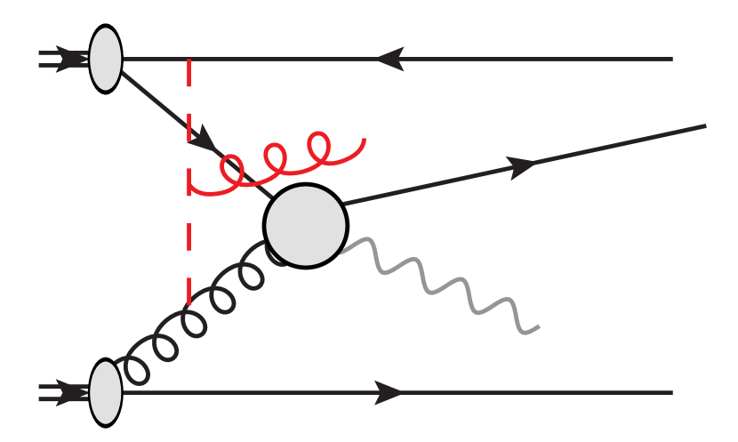
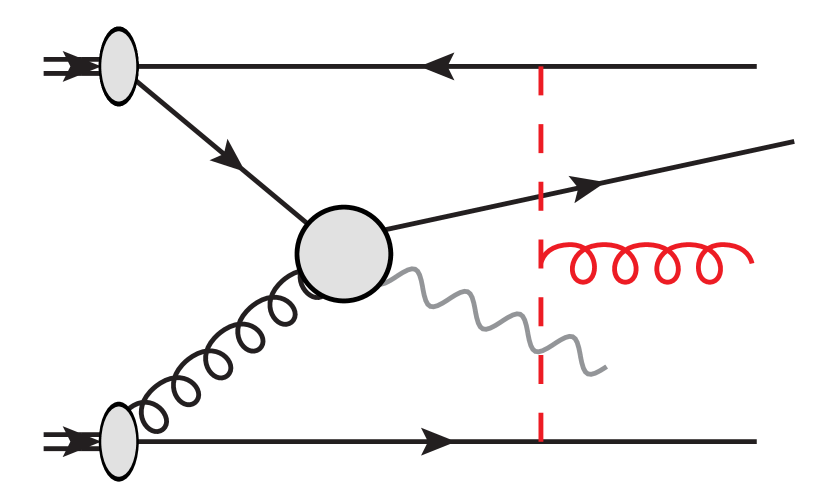
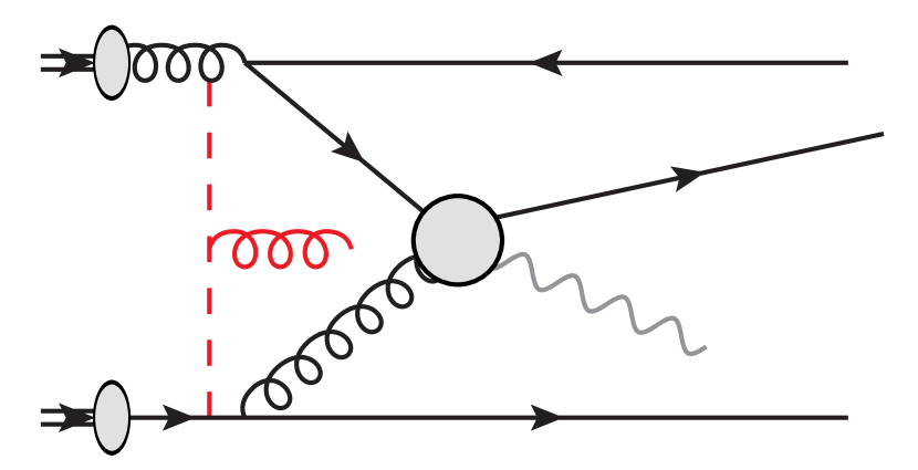
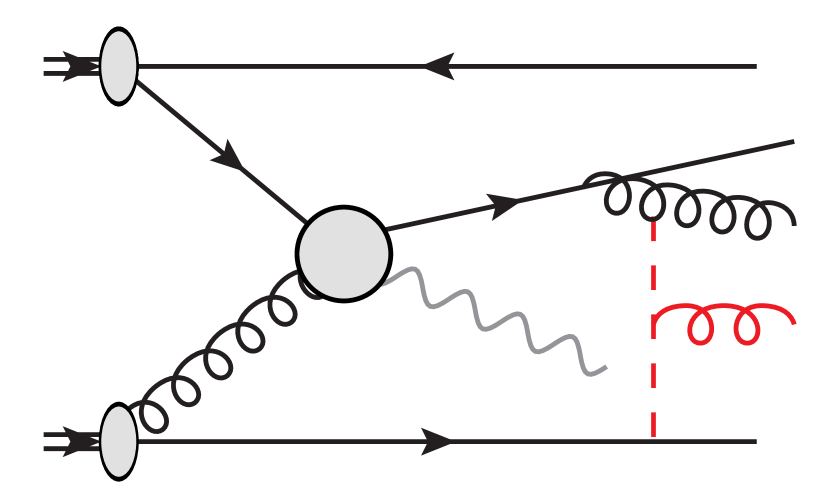
Moving on to the discussion of our case: We begin with Glauber exchanges involving Lipatov vertices off Glauber rungs connecting to at least one active parton, as e.g. in figure 2(a). Following ref. Rothstein:2016bsq , the Glauber exchange is an element of the soft or collinear sector, the Lipatov vertex therefore represents soft radiation off either another soft, or off a collinear emission. In the former case (the soft overlap for active-active Glauber exchange), this simply is the soft dynamics encoded in the soft Wilson line structure and Lagrangian. For the latter case, it corresponds to a soft emission off a collinear field, which does not appear in the SCET_II Lagrangian. Instead it has been integrated out and is thus accounted for in the matching of QCD to SCET, where a soft Wilson line is introduced for every collinear Wilson line. This soft Wilson line then accounts for the Lipatov emissions off the Glauber subset of the corresponding collinear Wilson line (besides other soft effects). This leaves us with Glauber exchanges between spectators only, which also have at least one Lipatov emission. It is clear that the lowest order that such diagrams could appear in the perturbative expansions is $\mathcal{O}(\alpha_{s}^{2})$.

Focusing on Glauber exchanges between the proton remnants, we naively expect that a contribution of the form of figure 2(b) could appear at $\mathcal{O}(\alpha_{s}^{2})$, when interfering with a suitable tree-level diagram. However, such interference is prohibited by momentum conservation: The proton remnants have transverse momenta of $\mathcal{O}(\Lambda_{\rm QCD})$, the typical scale of intra-proton dynamics, while the Glauber exchange represents a recoil between the involved spectators, causing them to have transverse momentum of $\mathcal{O}(q_{x})$. This does not match up with any tree level conjugate diagram. Accordingly, the conjugate amplitude also requires some perturbative exchange (Glauber or otherwise), which pushes the contribution to $\mathcal{O}(\alpha_{s}^{3})$. In addition, such diagrams do not contribute to our observable, as we only measure properties of the jet: Any recoil of beam remnants is never measured, and accompanying soft emissions are not relevant, because we use the WTA axis. For a diagram to have any effect it must impart recoil on the active partons or the jet constituents: The WTA axis follows a collinear emission in the jet, which can only pick up Glauber effects by direct recoil, or by inheriting recoil from the partons initiating the hard scattering.

An example for an allowed diagram would be figure 2(c), where a perturbative splitting of an initial state gluon creates spectators that already have transverse momentum of $\mathcal{O}(q_{T})$, such that a Glauber exchange does not fall prey to momentum conservation. Such diagrams appear, by virtue of the initial state branching, at the earliest at $\mathcal{O}(\alpha_{s}^{4})$. Lastly, we turn to diagrams involving the jet, like e.g. figure 2(d). As stated above, spectators in the jet can arise from perturbative splittings of the parton initiating the jet, which means such topologies start at $\mathcal{O}(\alpha_{s}^{3})$ at the lowest. Momentum conservation does not pose an obstacle here, as the soft emission across the cut can attach to the beam spectator in the conjugate amplitude, pushing its transverse momentum to the right scaling. However, an explicit calculation of the loop diagram in figure 2(d) shows that it evaluates to zero, as may have been expected due to its similarity with deep-inelastic scattering. Explicitly, as only two rapidity sectors are involved, we can boost to a frame in which they are back-to-back. Of the four non-Glauber propagators involving the loop momentum $k$, two will then depend only on $n\cdot k$, and two only on $\bar{n}\cdot k$, after expansions around the momentum scaling for Glauber and collinear modes. These two subsets correspond to the two collinear sectors, i.e. two propagators arise from the jet, the other from the beam remnant and active line. The two propagators arising from the jet have poles on the same side of the real line, and the loop integral thus evaluates to zero by residues. Numerator factors and the rapidity regulator do not change this outcome.

We thus conclude that effects of perturbative Glauber exchanges are suppressed by at least $\mathcal{O}(\alpha_{s}^{3})$ compared to the accuracy achieved in this paper.

4 Jet function calculations

4.1 Gluon jet function calculation at order $\alpha_{s}$

Next we present the calculation of the one-loop gluon jet functions. According to eq. (3.2), they are defined through

$$\mathscr{J}_{g}^{\mu\nu} \equiv\sum\limits_{j}[P_{n}^{\mu\nu}]^{j}_{g}\mathscr{J}^{j}_{g}(b_{x},\vec{p}_{T,J},\eta_{J},\epsilon)$$

$$=\frac{2(2\pi)^{d-1}}{N_{c}^{2}-1}\langle 0|\mathcal{B}_{n\perp}^{a\mu}(0)\left(0\right)e^{\mathrm{i}\delta_{x}b_{x}}\delta^{(2)}(\vec{p}_{T,J}-\hat{\vec{p}}_{T,J})\delta(y_{J}-\hat{y}_{J})\mathcal{B}_{n\perp}^{a\nu}(0)|0\rangle\;$$ (44)

where the transverse momentum of the jet with respect to the initial parton is encoded in

$$\delta_{x}=p_{x,c}-p_{x,J}.$$ (45)

In our original coordinates $p_{x,J}=0$, but we will instead perform our calculation in a frame where the total collinear momentum $p_{x,c}=0$. In this subsection we drop the subscript $J$ on light-cone coordinates for brevity. As discussed in sec. 2.1, the difference between $\vec{p}_{T,J}$ and $\vec{p}_{T,c}$ is $O(\lambda)$, so we can replace $\hat{\vec{p}}_{T,J}\to\vec{p}_{T,c}$, and similarly we can replace $y_{J}$ by $y_{c}$. Then, following the same steps as for the standard jet axis in ref. Chien:2019gyf , we can switch to coordinates along the momentum of the initial parton, to obtain

$$\mathscr{J}_{g}^{\mu\nu}= \frac{2(2\pi)^{d-1}}{N_{c}^{2}-1}\bar{n}\cdot p_{J}\langle 0|\mathcal{B}_{n\perp}^{a\mu}(0)e^{\mathrm{i}\delta_{x}{b}_{x}}\delta(\bar{n}\cdot p_{J}-\bar{n}\cdot p_{c})\delta^{(d-2)}(\vec{p}_{\perp,c})\mathcal{B}_{n\perp}^{a\nu}(0)|0\rangle.$$ (46)

Using the projectors in eq. (3.2), one finds at tree-level

$$\mathscr{J}_{g}^{T}=\frac{1}{d-2}[{P}_{n}^{\mu\nu}]^{T}_{g}\mathscr{J}_{g\mu\nu}=1+\mathcal{O}(\alpha_{s}),$$

$$\mathscr{J}_{g}^{L}=\frac{1}{(d-2)(d-3)}[{P}_{n}^{\mu\nu}]^{L}_{g}\mathscr{J}_{g\mu\nu}=\mathcal{O}(\alpha_{s}).$$ (47)

Figure 3: One-loop diagrams contributing to the gluon jet functions. The $\otimes$ denotes the collinear gluon field $\mathcal{B}_{n\perp}^{\mu}$ (dressed with Wilson lines).

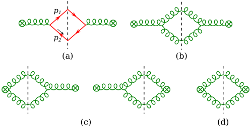
All one-loop diagrams for the gluon jet functions are shown in figure 3. The relevant Feynman rules for $\mathcal{B}^{\mu}_{n\perp}=\frac{1}{g}W_{n}^{\dagger}\mathrm{i}D_{n\perp}^{\mu}W_{n}$ are given by

$$\begin{array}[]{c}\includegraphics[width=52.03227pt]{Figures/BA.pdf}\end{array} =\frac{-\mathrm{i}\delta^{ab}}{p^{2}+\mathrm{i}0}\bigg{(}g_{\perp}^{\alpha\mu}-\frac{\bar{n}^{\alpha}p_{\perp}^{\mu}}{\bar{n}\cdot p-\mathrm{i}0}\bigg{)},$$ (49)

$$\begin{array}[]{c}\includegraphics[width=65.04034pt]{Figures/B2g.pdf}\end{array} =\mathrm{i}gf^{abc}\tilde{\mu}^{\epsilon}w^{2}\nu^{\eta}\bigg{[}g_{\perp}^{\alpha\mu}\frac{\bar{n}^{\beta}}{(\bar{n}\cdot p_{2})^{1+\eta}}-g_{\perp}^{\beta\mu}\frac{\bar{n}^{\alpha}}{(\bar{n}\cdot p_{1})^{1+\eta}}\bigg{]},$$ (51)

where $g$ is the renormalized coupling with $\tilde{\mu}^{2}=\mu^{2}e^{\gamma_{E}}/(4\pi)$, and we use the $\eta$-regulator Chiu:2011qc ; Chiu:2012ir to regularize rapidity divergences. The $w$ in eq. (49) is an (artificial) coupling used to derive the corresponding rapidity evolution. Diagram (d) vanishes in Feynman gauge, and the others contribute to the jet function according to,

$$\frac{\alpha_{s}}{4\pi}\,\mathscr{J}_{g}^{\mu\nu(1)}=\int{\rm d}\Pi_{2}\,e^{\mathrm{i}\delta_{x}b_{x}}\Bigl{[}n_{f}M_{a}^{\mu\nu}+\frac{1}{2}M_{b}^{\mu\nu}+\frac{1}{2}M_{c}^{\mu\nu}\Bigr{]}$$ (52)

where the $1/2$ is an identical particle factor and

$$M_{a}^{\mu\nu} =\frac{g^{2}T_{F}}{(p_{1}\cdot p_{2})^{2}}\tilde{\mu}^{2\epsilon}\big{(}-2p_{\perp}^{\mu}p_{\perp}^{\nu}-g_{\perp}^{\mu\nu}p_{1}\cdot p_{2}\big{)},$$

$$M_{b}^{\mu\nu} =\frac{g^{2}C_{A}}{(p_{1}\cdot p_{2})^{2}}\tilde{\mu}^{2\epsilon}\big{[}(d-2)p_{\perp}^{\mu}p_{\perp}^{\nu}+2g_{\perp}^{\mu\nu}p_{1}\cdot p_{2}\big{]},$$

$$M_{c}^{\mu\nu} =-\frac{g^{2}w^{2}C_{A}}{p_{1}\cdot p_{2}}\tilde{\mu}^{2\epsilon}\Bigl{(}\frac{\nu}{\omega_{J}}\Bigr{)}^{\eta}g_{\perp}^{\mu\nu}\bigg{[}\frac{1+z}{(1-z)^{1+\eta}}+\frac{2-z}{z^{1+\eta}}\bigg{]}\,.$$ (53)

with $p_{1}\cdot p_{2}=\vec{p}_{\perp}^{\,2}/(2z(1-z))$. The two-body collinear phase space entering in eq. (52), is defined as

$$\int{\rm d}\Pi_{2} \equiv 2(2\pi)^{d-1}\omega_{J}\prod\limits_{i=1}^{2}\int\frac{{\rm d}p_{i}^{-}{\rm d}^{d-2}p_{i\perp}}{2p_{i}^{-}(2\pi)^{d-1}}\,\delta(p^{-}_{J}-p_{1}^{-}-p_{2}^{-})\delta^{(d-2)}(\vec{p}_{1\perp}+\vec{p}_{2\perp})$$

$$=\frac{1}{4\pi}\int\frac{{\rm d}^{d-2}p_{\perp}}{(2\pi)^{d-2}}\int_{0}^{1}\frac{{\rm d}z}{z(1-z)}$$ (54)

which we rewrite in terms of the transverse momentum $\vec{p}_{\perp}$ and momentum fraction $z$,

$$\vec{p}_{\perp}=\vec{p}_{1\perp}=-\vec{p}_{2\perp},\qquad z=\frac{p_{1}^{-}}{p^{-}_{J}}=1-\frac{p_{2}^{-}}{p^{-}_{J}}.$$ (55)

The amplitudes in eq. (4.1) are also expressed in terms of these variables. For the WTA scheme, one has

$$\delta_{x}=\left\{\begin{array}[]{ll}-\frac{p_{x}}{1-z}&\text{for $\frac{1}{2}>z>0$}\\ \frac{p_{x}}{z}&\text{for $1>z>\frac{1}{2}$}\end{array}\right..$$ (58)

The evaluation of $\mathscr{J}_{g}^{i}$ involves the following two integrals

$$I_{1}(b_{x}) \equiv\int\frac{\mathrm{d}^{d-2}p_{\perp}}{(2\pi)^{d-2}}\frac{e^{\mathrm{i}b_{x}p_{x}}}{\vec{p}_{\perp}^{\,2}}=\frac{1}{4\pi}(\pi b_{x}^{2})^{\epsilon}\Gamma(-\epsilon),$$

$$I_{2}(b_{x}) \equiv\int\frac{\mathrm{d}^{d-2}p_{\perp}}{(2\pi)^{d-2}}\frac{p_{x}^{2}e^{\mathrm{i}b_{x}p_{x}}}{(\vec{p}_{\perp}^{\,2})^{2}}=\frac{1}{8\pi}(2\epsilon+1)(\pi b_{x}^{2})^{\epsilon}\Gamma(-\epsilon).$$ (59)

For $\mathscr{J}_{g}^{T}$, one has

$$\mathscr{J}_{g}^{T} =1-\frac{g_{\perp\mu\nu}}{d-2}\int\mathrm{d}\Pi_{2}\,e^{\mathrm{i}\delta_{x}b_{x}}\bigg{[}n_{f}M_{a}^{\mu\nu}+\frac{1}{2}M_{b}^{\mu\nu}+\frac{1}{2}M_{c}^{\mu\nu}\bigg{]}.$$ (60)

By using eq. (4.1) and eq. (4.1), this leads to

$$\mathscr{J}_{g}^{T} =1+\alpha_{s}\tilde{\mu}^{2\epsilon}\int_{0}^{1}\mathrm{d}z\,I_{1}\bigg{(}\frac{b_{x}}{\hat{z}}\bigg{)}\bigg{\{}w^{2}C_{A}\bigg{(}\frac{\nu}{\omega_{J}}\bigg{)}^{\eta}\bigg{[}\frac{1+z}{(1-z)^{1+\eta}}+\frac{2-z}{z^{1+\eta}}\bigg{]}$$

$$\qquad+2C_{A}[z(1-z)-1]+2T_{F}n_{f}\bigg{(}1-\frac{4}{d-2}z(1-z)\bigg{)}\bigg{\}}$$

$$=Z_{g}+\frac{\alpha_{s}}{4\pi}\bigg{[}C_{A}\bigg{(}4L_{b}\ln\frac{\nu}{\omega_{J}}+\frac{11}{3}L_{b}-\frac{2}{3}\pi^{2}+\frac{131}{18}-\frac{22}{3}\ln 2\bigg{)}+$$

$$\quad-T_{F}n_{f}\bigg{(}\frac{4}{3}L_{b}+\frac{17}{9}-\frac{8}{3}\ln 2\bigg{)}\bigg{]}\,,$$ (61)

where

$$\hat{z}=\max\{z,1-z\},\qquad L_{b}=\log\Bigl{(}\frac{b_{x}^{2}\mu^{2}}{4e^{-2\gamma_{E}}}\Bigr{)},\qquad\omega_{J}=2p_{T,J}\cosh\eta_{J},$$ (62)

and the jet function renormalization is

$$Z_{g}=1-\frac{\alpha_{s}C_{A}}{\pi\eta}w^{2}e^{(L_{b}-\gamma_{E})\epsilon}\Gamma(-\epsilon)+\frac{\alpha_{s}}{4\pi\epsilon}\bigg{[}C_{A}\bigg{(}4\ln\frac{\nu}{\omega_{J}}+\frac{11}{3}\bigg{)}-\frac{4}{3}n_{f}T_{F}\bigg{]}.$$ (63)

From this, one can easily obtain the one-loop anomalous dimensions

$$\Gamma_{\nu}^{\mathscr{J}_{g}}=\frac{\alpha_{s}C_{A}}{\pi}L_{b},$$

$$\Gamma_{\mu}^{\mathscr{J}_{g}}=\frac{\alpha_{s}}{2\pi}\bigg{[}C_{A}\bigg{(}4\ln\frac{\nu}{\omega_{J}}+\frac{11}{3}\bigg{)}-\frac{4}{3}n_{f}T_{F}\bigg{]}=2C_{A}\Gamma_{\text{cusp}}\ln\frac{\nu}{\omega_{J}}-2\gamma^{g}\,,$$ (64)

which agree with their all-order form in eq. (5.1).

For $\mathscr{J}_{g}^{L}$, one only needs to include the terms $\propto p_{\perp}^{\mu}p_{\perp}^{\nu}$ in eq. (4.1). It can then easily be evaluated by using the two integrals in eq. (4.1), yielding

$$\mathscr{J}_{g}^{L} =\frac{g^{2}}{2}\tilde{\mu}^{2\epsilon}\frac{(d-2){C_{A}}-4T_{F}n_{f}}{(d-2)(d-3)}\int\mathrm{d}\Pi_{2}\,\frac{e^{\mathrm{i}\delta_{x}b_{x}}}{(p_{1}\cdot p_{2})^{2}}\,[{P}_{n}^{\mu\nu}]^{L}_{g}\,p_{\perp}^{\mu}p_{\perp}^{\nu}$$ (65)

$$=2\alpha_{s}\tilde{\mu}^{2\epsilon}\frac{(d-2){C_{A}}-4T_{F}n_{f}}{(d-2)(d-3)}\int_{0}^{1}\mathrm{d}z\,z(1-z)\bigg{[}(d-2)I_{2}\bigg{(}\frac{b_{x}}{\hat{z}}\bigg{)}-I_{1}\bigg{(}\frac{b_{x}}{\hat{z}}\bigg{)}\bigg{]}.$$

Since

$$(d-2)I_{2}\bigg{(}\frac{b_{x}}{\hat{z}}\bigg{)}-I_{1}\bigg{(}\frac{b_{x}}{\hat{z}}\bigg{)}=-\frac{1}{4\pi}+\mathcal{O}(\epsilon),$$ (66)

$\mathscr{J}_{g}^{L}$ is finite at this order (as required, since it vanishes at tree-level). It is given by

$$\mathscr{J}_{g}^{L}=-\frac{\alpha_{s}}{4\pi}(2C_{A}-4T_{F})\int_{0}^{1}z(1-z)=\frac{\alpha_{s}}{4\pi}\Bigl{(}-\frac{1}{3}C_{A}+\frac{2}{3}T_{F}n_{f}\Bigr{)}.$$ (67)

4.2 Recombination scheme dependence

The WTA algorithm is not the only recombination scheme that can be used to construct a recoil-free jet axis. In this subsection we will employ a more general recombination scheme. It turns out that this only changes the finite part of the jet function, and at the end of this section we give explicit results.

A recombination scheme dictates how particles are merged during the clustering procedure. The simplest is to add the momentum four-vectors, which is known as the $E$-scheme. In the rest of this paper we focus on the WTA-scheme, specifically the WTA-$p_{T}$-scheme, described in section 2.1. Here, we consider a generalization in which the momenta $p_{i}$ and $p_{j}$ of two particles (or pseudojets) are recombined into $p_{r}$ as follows

$$p_{T,r} =p_{T,i}+p_{T,j},$$

$$\phi_{r} =(p_{T,i}^{n}\phi_{i}+p_{T,j}^{n}\phi_{j})/(p_{T,i}^{n}+p_{T,j}^{n}),$$

$$y_{r} =(p_{T,i}^{n}y_{i}+p_{T,j}^{n}y_{j})/(p_{T,i}^{n}+p_{T,j}^{n}),$$ (68)

in terms for the transverse momentum $p_{T}$, azimuthal angle $\phi$ and rapidity $y$. The azimuthal angle and rapidity are combined in a way that favors the direction of the harder particle, with the weight of the factors $p_{T,i}^{n}$ controlled by the power of $n\geq 1$. For $n>1$ this recombination scheme is recoil free, implying that the same factorization theorem holds as for the WTA scheme (which corresponds to $n\to\infty$). Since only the jet function depends on $n$, consistency of the factorization implies that only the constant term of the jet function depends on it, which is borne out by an explicit calculation.

Now, let us calculate gluon jet functions at one loop using the general scheme in eq. (4.2). For two collinear partons, using coordinates along the parton that initiates the jet, one has $\phi_{i}\approx p_{x,i}/p_{T,i}$ and $p_{x}=p_{x,1}=-p_{x,2}$ such that 

$$\delta_{x} =p_{T,J}\frac{p_{T,1}^{n}\phi_{1}-p_{T,2}^{n}\phi_{2}}{p_{T,1}^{n}+p_{T,2}^{n}}=p_{J}^{-}\frac{(p_{1}^{-})^{n}\frac{p_{x}}{p_{1}^{-}}-(p_{2}^{-})^{n}\frac{p_{x}}{p_{2}^{-}}}{({p_{1}^{-}})^{n}+({p_{2}^{-}})^{n}}=\frac{z^{n-1}-(1-z)^{n-1}}{z^{n}+(1-z)^{n}}\,p_{x}$$ (69)

in terms of the kinematic variables in eq. (55). As a consistancy check, one can easily see that $\delta_{x}$ reduces to the expression for the WTA axis in eq. (58) in the limit $n\to\infty$. With the following replacement

$$\hat{z}\to\hat{z}_{n}=\bigg{|}\frac{z^{n}+(1-z)^{n}}{z^{n-1}-(1-z)^{n-1}}\bigg{|},$$ (70)

one can straightforwardly evaluate the gluon jet functions for the general recombination scheme by extending the calculation in the previous section.

Figure 4: Finite part (i.e. $L_{b}=0$) of the contributions from gluons ($J_{C_{A}}$) and quarks ($J_{n_{f}}$) to the gluon and to the quark ($J_{C_{F}}$) jet function for the recombination scheme in eq. (4.2) with $n>1$. The results for the WTA scheme (black dashed lines) are approached for $n\to\infty$. $J_{C_{A}}$, $J_{n_{f}}$ and $J_{C_{A}}$ are defined in eq. (4.2) and eq. (77), respectively.

For $\mathscr{J}_{g}^{L}$, one can easily see that eq. (67) is valid for all the values of $n$ because the dependence on $\hat{z}_{n}$ drops out in eq. (66). $\mathscr{J}_{g}^{T}$ is given by the first two lines of eq. (4.1) with the replacement for $\hat{z}_{n}$ in eq. (70). The $1/\eta$ pole arises only from the following expansions

$$\frac{1}{(1-z)^{1+\eta}}\to-\frac{1}{\eta}\delta(1-z),\text{ and }\frac{1}{z^{1+\eta}}\to-\frac{1}{\eta}\delta(z)$$ (71)

in the integrand of eq. (4.1). Since

$$I_{1}\bigg{(}\frac{b_{x}}{\hat{z}_{n}}\bigg{)}\bigg{|}_{z=\text{0 or 1}}=I_{1}(b_{x}),$$ (72)

the $\hat{z}_{n}$-dependence drops out and the $1/\eta$ term is the same as for the WTA Scheme. Similarly, the only source for the $1/\epsilon$ pole in $\mathscr{J}_{g}^{T}$ comes from the pole in $I_{1}$ with

$$\Bigl{(}\frac{\mu^{2}e^{\gamma_{E}}}{4\pi}\Bigr{)}^{\epsilon}I_{1}\bigg{(}\frac{b_{x}}{\hat{z}_{n}}\bigg{)}=-\frac{1}{4\pi}\bigg{[}\frac{1}{\epsilon}+L_{b}-\ln(\hat{z}_{n}^{2})\bigg{]}+\mathcal{O}(\epsilon).$$ (73)

Hence, the jet function renormalization in eq. (63) and the anomalous dimensions in eq. (4.1) are valid for any value of $n>1$, as required by consistency of the factorization. By using the expansion in eq. (73), we obtain the constant term of $\mathscr{J}_{g}^{T}$ (i.e. taking $L_{b}=0$)

$$\mathscr{J}_{g}^{T}\bigr{|}_{L_{b}=0} =1+\frac{\alpha_{s}}{2\pi}\bigg{\{}C_{A}\int_{0}^{1}\mathrm{d}z\,\ln(\hat{z}_{n}^{2})\bigg{[}\frac{z}{1-z}+\frac{1-z}{z}+z(1-z)\bigg{]}$$

$$\quad+T_{F}n_{f}\bigg{[}\frac{1}{3}+\int_{0}^{1}\mathrm{d}z\,\ln(\hat{z}_{n}^{2})((1-z)^{2}+z^{2})\bigg{]}\bigg{\}}$$

$$\equiv 1+\frac{\alpha_{s}}{4\pi}(C_{A}J_{C_{A}}+T_{F}n_{f}J_{n_{f}})$$ (74)

For $n\to\infty$, it reproduces that for the WTA scheme:

$$J_{C_{A}}|_{n\to\infty}=\frac{131}{18}-\frac{22\ln 2}{3}-\frac{2\pi^{2}}{3}\,,\quad J_{n_{f}}|_{n\to\infty}=\frac{8\ln 2}{3}-\frac{17}{9}.$$ (75)

One can also find analytic results for specific values of $n$. E.g. for the $p_{t}^{2}$ scheme ($n=2$), we have

$$J_{C_{A}}|_{n=2}=\frac{58}{9}-\frac{10\pi}{3}+\pi^{2}\,,\quad J_{n_{f}}|_{n=2}=\frac{2\pi}{3}-\frac{2}{9}\,.$$ (76)

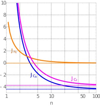
The two constants $J_{C_{A}}$ and $J_{n_{f}}$ are plotted as function of $n$ in figure 4. The analytic result for the WTA scheme is also shown, and one can see that it is approached in the limit $n\to\infty$. For $n=1$ the jet is no longer recoil-free. This is reflected in a diverging constant in the $n\to 1$ limit, indicating that the poles of the jet function, and thus the entire factorization are different for $n=1$. Similarly, the finite part of $\mathscr{J}_{q}$ in general depends on $n$ and takes the form

$$\mathscr{J}_{q}\bigr{|}_{L_{b}=0}= 1+\frac{\alpha_{s}C_{F}}{4\pi}\bigg{[}1+2\int_{0}^{1}\mathrm{d}z\,\ln(\hat{z}_{n}^{2})\frac{1+z^{2}}{1-z}\bigg{]}\equiv 1+\frac{\alpha_{s}C_{F}}{4\pi}J_{C_{F}}\,.$$ (77)

In figure 4, $J_{C_{F}}$ is also shown. For the $p_{t}^{2}$ scheme and for the WTA scheme,

$$J_{C_{F}}\bigr{|}_{n=2}=7-3\pi+\pi^{2}\,,\qquad J_{C_{F}}\bigr{|}_{n\to\infty}=7-\frac{2\pi^{2}}{3}-6\ln 2\,.$$ (78)

4.3 Track-based jet function

Next, we will consider the case where the jet is measured using only charged particles, exploiting the superior angular resolution of the tracking system. Since this does not modify the effect of soft radiation on the measurement, which still contributes through the total recoil, this only affects the jet function. This is similar to the different recombination schemes considered in sec. 4.2, and we can reuse much of the calculation, though we will restrict ourselves to the effect of a track-based measurement for WTA scheme. In particular, the jet function anomalous dimensions are not modified but only the constant, which should be contrasted with the complicated jet function encountered for a track-based measurement of thrust in ref. Chang:2013iba .

We will account for the conversions of the partons to charged particles using the track function formalism Chang:2013rca ; Chang:2013iba . At one-loop order, the jet consists of (at most) two partons and for $q_{x}\gg\Lambda_{\rm QCD}$ they can be treated as fragmenting independently into charged hadrons moving in the same direction as the original partons. Denoting the total momentum fractions of charged hadrons produced by each of the two partons by $z_{1}$ and $z_{2}$, the only change due to a track-based measurement is that the condition which parton “wins” gets modified:

$$\hat{z}=\max\{z,1-z\}\quad\to\quad\hat{z}_{\rm ch}=\left\{\begin{tabular}[]{ll}$z$&$z_{1}z>z_{2}(1-z)$\\ $1-z$&$z_{1}z<z_{2}(1-z)$\end{tabular}\right.\,.$$ (81)

We also need to take into account the nonperturbative distribution of $z_{1}$ (and $z_{2}$) which is described by a track function $T_{f}(z_{1},\mu)$, where $f$ is the flavor of the parton. For example, for the gluon jet function in eq. (52), the corresponding track-based measurement (indicated by the bar) is

$$\frac{\alpha_{s}}{4\pi}\,\bar{\mathscr{J}}_{g}^{\mu\nu(1)} =\int\!\mathrm{d}z_{1}\mathrm{d}z_{2}\int{\rm d}\Pi_{2}\,e^{\mathrm{i}\delta_{x,{\rm ch}}b_{x}}\Bigl{[}\sum_{q}T_{q}(z_{1})T_{q}(z_{2})M_{a}^{\mu\nu}+T_{g}(z_{1})T_{g}(z_{2})\frac{1}{2}M_{b}^{\mu\nu}$$

$$\quad+T_{g}(z_{1})T_{g}(z_{2})\frac{1}{2}M_{c}^{\mu\nu}\Bigr{]}\,,$$ (82)

where $|\delta_{x,{\rm ch}}|=|p_{x}|/\hat{z}_{\rm ch}$, and the track functions depend on the flavor of the partons in the final state. Note that different quark flavors have different track functions, but $T_{q}=T_{\bar{q}}$ due to charge conjugation invariance.

The subsequent steps directly parallel those in sec. 4.2, so we find again that the one-loop jet function for the linearly-polarized gluon $\bar{\mathscr{J}}_{g}^{L}$ is not modified, while for the transversely-polarized gluon and quark we have

$$\bar{\mathscr{J}}_{g}^{T}\bigr{|}_{L_{\perp}=0} =1+\int\!\mathrm{d}z_{1}\mathrm{d}z_{2}\,\frac{\alpha_{s}}{2\pi}\bigg{\{}T_{g}(z_{1})T_{g}(z_{2})\,C_{A}\int_{0}^{1}\mathrm{d}z\,\ln(\hat{z}_{\rm ch}^{2})\bigg{[}\frac{z}{1-z}+\frac{1-z}{z}+z(1-z)\bigg{]}$$

$$\quad+\sum_{q}T_{q}(z_{1})T_{q}(z_{2})T_{F}\bigg{[}\frac{1}{3}+\int_{0}^{1}\mathrm{d}z\,\ln(\hat{z}_{\rm ch}^{2})((1-z)^{2}+z^{2})\bigg{]}\bigg{\}}\,,$$

$$\bar{\mathscr{J}}_{q}\bigr{|}_{L\perp=0} =1+\int\!\mathrm{d}z_{1}\mathrm{d}z_{2}\,T_{q}(z_{1})T_{g}(z_{2})\frac{\alpha_{s}C_{F}}{4\pi}\bigg{[}1+2\int_{0}^{1}\mathrm{d}z\,\ln(\hat{z}_{\rm ch}^{2})\frac{1+z^{2}}{1-z}\bigg{]}\,,$$ (83)

in direct analogy to eqs. (4.2) and (77).

5 Resummation and matching

5.1 Renormalization group evolution

In section 3 we have given the derivation of the factorization formula and the explicit expressions for the one-loop ingredients. Within the EFT framework one then uses the renormalization group (RG) evolution equations to resum the large logarithms between different scales. In addition to the standard UV divergences regularized by the dimensional regularization, the jet, beam and soft functions also involve rapidity divergences, as these modes are not separated in invariant mass but rapidity, see eq. (6). In order to resum the corresponding rapidity logarithms we apply the rapidity RG method developed in ref. Chiu:2011qc ; Chiu:2012ir . Different regulator choices (e.g. Collins:2011zzd ; Chiu:2009yx ; Becher:2011dz ; Echevarria:2015byo ; Li:2016axz ; Ebert:2018gsn ) or resummation via the collinear anomaly framework Becher:2011pf ; Becher:2010tm are also possible and (up to the possibility of scale variation) equivalent. To achieve next-to-next-to-leading logarithmic resummation, we need the one-loop fixed order ingredients in sec. 3.3 and the two-loop anomalous dimensions (except for the cusp term in the anomalous dimensions, which is required at three loop order).

Generally, the RG equations for a function $F$ are given by

$$\frac{\mathrm{d}}{\mathrm{d}\ln\mu}F(\mu)=\Gamma^{F}_{\mu}F(\mu),\quad\frac{\mathrm{d}}{\mathrm{d}\ln\nu}F(\mu,\nu)=\Gamma^{F}_{\nu}F(\mu,\nu).$$ (84)

where $\Gamma_{\mu}^{F}$ and $\Gamma_{\nu}^{F}$ denote the standard and rapidity anomalous dimensions, respectively. For the beam, jet and soft function, this multiplicative form of the evolution equation only holds in impact parameter space, and the anomalous dimension depends on $b_{x}$. In addition the anomalous dimension may e.g. depend on the hard kinematics or the jet direction, which we omit.

The anomalous dimension of the hard function are

$$\Gamma_{\mu}^{{\cal H}_{ij\to Vk}}=\Gamma_{\rm cusp}(\alpha_{s})\Big{(}C_{i}\ln\frac{\hat{u}^{2}}{p_{T,V}^{2}\mu^{2}}+C_{j}\ln\frac{\hat{t}^{2}}{p_{T,V}^{2}\mu^{2}}+C_{k}\ln\frac{p_{T,V}^{2}}{\mu^{2}}\Big{)}+2\big{(}\gamma_{\mu}^{i}+\gamma_{\mu}^{j}+\gamma_{\mu}^{k}\big{)}(\alpha_{s})\,,$$ (85)

where $C_{i}$ and $\gamma_{\mu}^{i}$ are the color factor and non-cusp anomalous dimension for parton $i$, i.e. $C_{A}$ and $\gamma_{\mu}^{g}$ for a gluon, and $C_{F}$ and $\gamma_{\mu}^{q}$ for an (anti-)quark. As we always have (up to permutation) two quarks and a gluon in our process, the non-cusp anomalous part simplifies to $\sum_{a}\gamma_{\mu}^{a}=2\gamma_{\mu}^{q}+\gamma_{\mu}^{g}$. The expressions for the partonic Mandelstam variables in terms of the kinematics of the boson and jet are collected in eq. (3.3). The perturbative expansion for $\Gamma_{\rm cusp}$ and $\gamma^{a}_{\mu}$ have been collected in appendix A.

The anomalous dimensions of the beam functions are

$$\Gamma_{\mu}^{B_{i}}(\alpha_{s})=2C_{i}\Gamma_{\rm cusp}(\alpha_{s})\ln\frac{\nu}{\omega_{i}}+\gamma_{\mu}^{B_{i}}(\alpha_{s})\,,$$

$$\Gamma_{\nu}^{B_{i}}(\alpha_{s})=2C_{i}A_{\Gamma_{\rm cusp}}(\mu,\mu_{B})-C_{i}\frac{\gamma_{\nu}(\alpha_{s})}{2}$$ (86)

where $\omega_{i}$ is explicitly defined in eq. (36), $\mu_{B}=2/e^{\gamma_{E}}b_{x}$ (so $L_{b}=\ln\mu^{2}/\mu_{B}^{2}$), and the cusp anomalous dimension $\Gamma_{\rm cusp}$, non-cusp anomalous dimension $\gamma^{B_{i}}_{\mu}$, and rapidity anomalous dimension $\gamma_{\nu}$ in appendix A. The function $A_{\Gamma_{\rm cusp}}$ is obtained by replacing $\gamma^{i}\to\Gamma_{\rm cusp}$ in $A_{\gamma^{i}}$ in eq. (113). The jet function $\mathscr{J}$ satisfies the same anomalous dimension as the beam function, where now $\omega_{J}=\bar{n}_{J}\cdot p_{J}=2p_{T,J}\cosh\eta_{J}$.

The anomalous dimensions of the soft function are

$$\Gamma_{\mu}^{S_{ijk}}(\alpha_{s}) =\Gamma_{\rm cusp}(\alpha_{s})\biggl{[}\left(C_{i}+C_{j}+C_{k}\right)\ln\frac{\mu^{2}}{\nu^{2}}-C_{i}\ln\frac{\alpha_{ji}\alpha_{ik}}{\alpha_{jk}}-C_{j}\ln\frac{\alpha_{ij}\alpha_{jk}}{\alpha_{ik}}$$ (87)

$$\quad-C_{k}\ln\frac{\alpha_{ik}\alpha_{kj}}{\alpha_{ij}}\biggr{]}+(C_{i}+C_{j}+C_{k})\gamma_{\mu}^{S}(\alpha_{s})$$

$$\Gamma_{\nu}^{S_{ijk}}(\alpha_{s}) =-2(C_{i}\!+\!C_{j}\!+\!C_{k})A_{\Gamma_{\rm cusp}}(\mu,\mu_{B})+(C_{i}\!+\!C_{j}\!+\!C_{k})\frac{\gamma_{\nu}(\alpha_{s})}{2}$$

with

$$\alpha_{ij}\equiv\frac{n_{i}\cdot n_{j}}{2}.$$ (88)

From eqs. (85), (5.1), (87) and the non-cusp anomalous dimensions in appendix A, it is straightforward to verify that the factorized cross section in (3.1) is independent of the renormalization scale $\mu$ and rapidity renormalization scale $\nu$:

$$\gamma_{\mu}^{{\cal H}_{ij\to Vk}}(\alpha_{s})+\gamma_{\mu}^{S_{ijk}}(\alpha_{s})+\gamma_{\mu}^{B_{i}}(\alpha_{s})+\gamma_{\mu}^{B_{j}}(\alpha_{s})+\gamma_{\mu}^{\mathscr{J}_{k}}(\alpha_{s}) =0\,,$$

$$\gamma_{\nu}^{S_{ijk}}(\alpha_{s})+\gamma_{\nu}^{B_{i}}(\alpha_{s})+\gamma_{\nu}^{B_{j}}(\alpha_{s})+\gamma_{\nu}^{\mathscr{J}_{k}}(\alpha_{s}) =0\,.$$ (89)

Figure 5: We evolve all ingredients from their natural $(\mu,\nu)$ scale to the scale of the soft function along the indicated paths. We take the different $\nu_{i}$ into account though they are of the same parametric size.

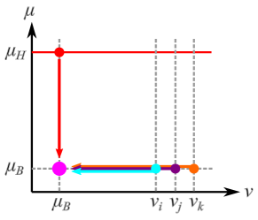
Using the renormalization group equations to evolve all ingredients in eq. (3.1) from their natural $\mu$ and $\nu$ scales to a common scale, the all-order resummation formula can be written as

$$\frac{\mathrm{d}\sigma_{\text{resum }}}{\mathrm{d}q_{x}\,\mathrm{d}p_{T,V}\mathrm{d}y_{V}} =\sum_{ijk}\int_{0}^{\infty}\frac{\mathrm{d}b_{x}}{\pi}\,\cos(b_{x}q_{x})\prod_{a=ijk}\Bigl{(}\frac{\nu_{S}}{\nu_{a}}\Bigr{)}^{\Gamma_{\nu}^{B_{a}}(\mu_{B})}\exp\biggl{(}\int^{\mu_{B}}_{\mu_{H}}\frac{\mathrm{d}\mu}{\mu}\Gamma_{\mu}^{\mathcal{H}_{ij}\rightarrow Vk}(\alpha_{s})\biggr{)}$$

$$\quad\times\mathcal{H}_{ij\rightarrow kV}(p_{T,V},y_{V}-\eta_{J},\mu_{H})\mathcal{B}_{i}(x_{1},b_{x},\mu_{B},\nu_{i})\mathcal{B}_{j}(x_{2},b_{x},\mu_{B},\nu_{j})$$

$$\quad\times\mathscr{J}_{k}(b_{x},\mu_{B},\nu_{k})S_{ijk}(b_{x},\mu_{B},\nu_{S})\,,$$ (90)

where we use $i$ to label the parton flavor but also the rapidity scales of the beams and jets, and understand $\Gamma_{\nu}^{B_{k}}$ to refer to the jet function rapidity anomalous dimension. We chose to evolve the beam and jet function from their natural rapidity scales $\nu_{i}$ to the rapidity scale $\nu_{S}$ of the soft function at the common invariant mass scale $\mu_{B}$, and evolve the hard function from $\mu_{H}$ down to the scale $\mu_{B}$, as summarized in figure 5. The evolution factor can be evaluated analytically as

$$\exp\biggl{(}\int_{\mu_{H}}^{\mu_{B}}\frac{\mathrm{d}\mu}{\mu}\Gamma_{\mu}^{\mathcal{H}_{ij}\rightarrow Vk}(\alpha_{s})\biggr{)}$$

$$\quad=\biggl{(}\frac{\hat{u}^{2}}{p_{T,V}^{2}\mu_{H}^{2}}\biggr{)}^{-C_{i}A_{\Gamma_{\rm cusp}}(\mu_{H},\mu_{B})}\biggl{(}\frac{\hat{t}^{2}}{p_{T,V}^{2}\mu_{H}^{2}}\biggr{)}^{-C_{j}A_{\Gamma_{\rm cusp}}(\mu_{H},\mu_{B})}\biggl{(}\frac{p_{T,V}^{2}}{\mu_{H}^{2}}\biggr{)}^{-C_{k}A_{\Gamma_{\rm cusp}}(\mu_{H},\mu_{B})}$$

$$\qquad\times\exp\Bigl{[}2(C_{i}+C_{j}+C_{k})S(\mu_{H},\mu_{B})-2\sum_{a=ijk}A_{\gamma^{a}}(\mu_{H},\mu_{B})\Bigr{]}.$$ (91)

The functions $A$ and $S$ are given in appendix A. The natural scales for the various ingredients in the resummation formula are taken to be

$$\mu_{H}=\sqrt{m_{V}^{2}+p_{T,V}^{2}}\,,~{}~{}~{}\mu_{B}=\nu_{S}=2e^{-\gamma_{E}}/b_{*},~{}~{}~{}\nu_{a}=\omega_{a}=\bar{n}_{a}\cdot p_{a}\,,$$ (92)

where we avoid unphysical results in the large-$b$ region, by applying the $b_{*}$-prescription Collins:1984kg

$$b_{*}=|b_{x}|/\sqrt{1+b_{x}^{2}/b_{\rm max}^{2}}\,,$$ (93)

with $b_{\rm max}=1.5\,{\rm GeV}^{-1}$.

Figure 6: Uncertainties estimated by varying the renormalization scale $\mu_{B}$ (left) and $\mu_{H}$ (right) up and down by a factor of 2. The rapidity scale variation is not shown, as it is negligible for our central scale choice for $\mu_{B}$.

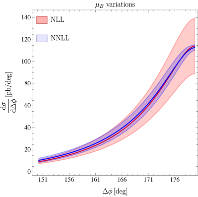
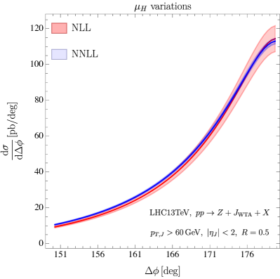
In figure 6 we show the resummation results at NLL and NNLL accuracy, separately displaying the various contributions to the perturbative uncertainties. Specifically, we assess the uncertainties by varying $\mu_{H}$, $\mu_{B}$ and $\nu_{S}$ up and down by a factor of two around their default values in (92). The fact that the uncertainty band is smaller at NNLL than at NLL, and that the bands overlap over almost the entire range, suggest that this is a reasonable estimate. In our full result we will combine these uncertainties by taking the envelope.

To model non-perturbative corrections, we furthermore will include the multiplicative function $e^{-S_{\rm NP}(b)}$

$$e^{-S_{\rm NP}(b_{x})}=e^{-g_{1}b_{x}^{2}}\prod_{a=ijk}\exp\Bigl{(}-\frac{C_{a}}{C_{F}}\frac{g_{2}}{2}\ln\frac{|b_{x}|}{b_{*}}\ln\frac{\omega_{a}}{Q_{0}}\Bigr{)}\,.$$ (94)

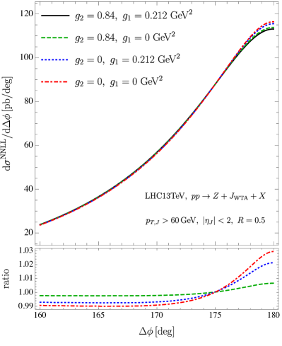
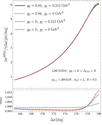
We take the same nonperturbative function $S_{\rm NP}$ as for transverse momentum distributions in Su:2014wpa , assuming that the nonperturbative contribution to the rapidity anomalous dimension (with coefficient $g_{2}$) can be obtained for a gluon beam or jet function by Casimir scaling. It is not clear whether this should also be the case for the nonperturbative model (with parameter $g_{1}$) and we take it the same for quark and gluon beams/jets, finding that it has a negligible effect on numerics anyway. We will use the results for the nonperturbative parameters obtained in ref. Su:2014wpa : $Q_{0}^{2}=2.4~{}{\rm GeV}^{2}$, $g_{1}=0.212~{}{\rm GeV}^{2}$ and $g_{2}=0.84$. The sensitivity of our predictions to these nonperturbative parameters is explored in figure 7, finding minimal sensitivity to $g_{1}$ but sensitivity to $g_{2}$ at the percent level in the region of $\Delta\phi\sim\pi$.

Figure 7: Variations of the nonperturbative parameters $g_{1}$ and $g_{2}$ in (94) for different jet transverse momentum cuts: $p_{T,J}>60\,{\rm GeV}$ (left) and $p_{T,J}>200\,{\rm GeV}$ (right).

5.2 Matching to fixed-order MCFM

In the back-to-back region where $\delta\phi\to 0$ ($\Delta\phi\to\pi$), the resummation formula will cure the divergence behavior of fixed-order results. However, if $\delta\phi$ is not small, the factorization formula receives large corrections of powers of $\delta\phi$. In this region, the resummation should be switched off, since $\ln\delta\phi$ is no longer large, and we therefore need to use fixed-order calculations that include these power corrections.

We use an additive matching scheme, in which the “naive” matched result of NNLL resummed prediction and the fixed-order can be obtained by the following relation

$$\mathrm{d}\sigma_{\rm naive}(\mathrm{NLO}+\mathrm{NNLL})=\mathrm{d}\sigma(\mathrm{NNLL})+\underbrace{\mathrm{d}\sigma(\mathrm{NLO})-\mathrm{d}\sigma(\mathrm{NLO}\text{ singular})}_{{\rm d}\sigma({\rm NLO}~{}{\rm non-singular})},$$ (95)

where we use MCFM Campbell:2002tg ; Campbell:2003hd to calculate the NLO results. The NLO singular distribution removes the overlap between the first two terms and can be obtained by expanding the resummation formula (5.1) to $\mathcal{O}(\alpha_{s})$. The NLO non-singular distribution is given by the difference between NLO and NLO singular results, as indicated in the above definition.

In principle, as $\delta\phi$ becomes large, the NNLL resumed cross section reduces to the NLO singular, leading to a cancellation between the first and third term in eq. (95). However, as is clear from (5.1), the numerical Fourier transformation from $b$-space to the momentum space rapidly oscillates when the resummation turns off and the evolution factor approaches $1$. To avoid the corresponding numerical instability, we apply a transition function $t(\Delta\phi)$ as follows:

$$\mathrm{d}\sigma(\mathrm{NLO}+\mathrm{NNLL})=[1-t(\Delta\phi)]\mathrm{d}\sigma_{\rm naive}(\mathrm{NLO}+\mathrm{NNLL})+t(\Delta\phi)\mathrm{d}\sigma(\mathrm{NLO})\,$$ (96)

The transition function we use is defined as

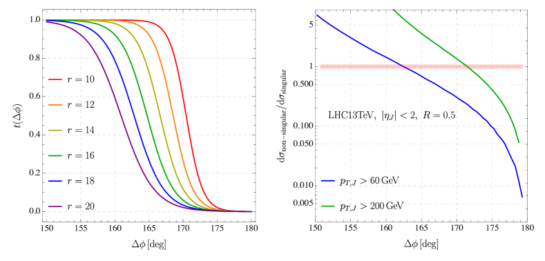
$$t(\Delta\phi)=\frac{1}{2}-\frac{1}{2}\tanh\Bigl{[}4-\frac{240(\pi-\Delta\phi)}{r}\Bigr{]},$$ (97)

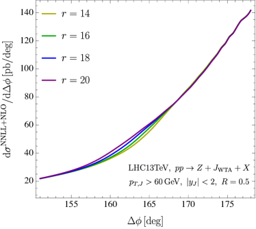
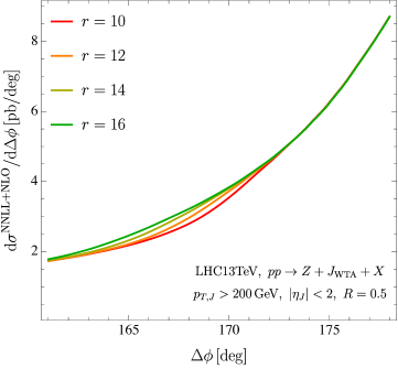
where the parameter $r$ fixes the transition point to be at approximately $180-r$ degrees. Different choices of $r$ are illustrated in the left panel of figure 8. In the right panel we show the difference of the NLO and NLO singular cross section, divided by the NLO singular. This indicates that the power corrections to our factorization theorem are order one around $\Delta\phi$ of $160^{\rm o}$ and $170^{\rm o}$ for $p_{T,J}>60$ GeV (blue curves) and $p_{T,J}>200$ GeV (green curves), respectively, which leads us to choose $r=20$ and $10$ in these two kinematic regions. The dependence on the choice of transition point $r$ is shown in figure 9. The nonsingular is in principle much smaller than the singular, but because the singular is resummed, there is less of a difference between them. Therefore we can see a sizable effect on how the nonsingular correction is treated in the resummation region, particularly when the jet $p_{T}$ is large. We will discuss the origin of this large nonsingular correction in sec. 6.2, arguing that it should not be Sudakov suppressed in the back-to-back limit, which is why we use an additive rather than multiplicative matching.

Figure 8: Left: the transition function defined in (96) with transition points at approximately $180-r$ degrees with $r=10$, $12$, $14$, $16$, $18$ and $20$. Right: the NLO non-singular divided by the NLO singular, indicating the appropriate choice of transition point.

Figure 9: Varying the transition point in matching our NNLL resummation to the NLO for $p_{T,J}>60$ GeV (left) and 200 GeV (right).

We conclude this section by presenting expressions for the NLO singular at the level of the integrated cross section,

$$\Sigma_{\rm singular}(\delta\phi^{\rm cut})=\int_{0}^{\delta\phi^{\rm cut}}\!\!\mathrm{d}(\delta\phi)\frac{\mathrm{d}\sigma}{\mathrm{d}(\delta\phi)\,\mathrm{d}p_{T,V}\mathrm{d}y_{V}}\,.$$ (98)

At order $\alpha_{s}$ we have

$$\Sigma^{(1)}_{\rm singular}(\delta\phi^{\rm cut}) =\sum_{ab}\int_{x_{1}}^{1}\frac{\mathrm{d}z_{1}}{z_{1}}f_{a/p}(x_{1}/z_{1},\mu)\int_{x_{2}}^{1}\frac{\mathrm{d}z_{2}}{z_{2}}f_{b/p}(x_{2}/z_{2},\mu)$$

$$\quad\times\sum_{ijk}\Bigl{(}\mathcal{H}_{ij\to Vk}^{(0)}C_{ij\leftarrow ab}^{(1)}+\mathcal{H}_{ij\to Vk}^{L,(0)}C_{ij\leftarrow ab}^{L,(1)}\Bigr{)}\,.$$ (99)

The first term on the second line is the contribution from the unpolarized gluon beam/jet functions, while the second term is the linearly-polarized contribution, as indicated by the superscript $L$. The one-loop coefficients are given by

$$C^{(1)}_{ij\leftarrow ab} =A_{ij}\delta_{ia}\delta_{jb}\delta(1-z_{1})\delta(1-z_{2})+\delta(1-z_{2})\delta_{jb}\left[4P_{ia}(z_{1})\left(L-\ln\frac{\mu}{2p_{T}}\right)+R_{ia}(z_{1})\right]$$

$$\quad+\delta(1-z_{1})\delta_{ia}\left[4P_{jb}(z_{2})\left(L-\ln\frac{\mu}{2p_{T}}\right)+R_{jb}(z_{2})\right]$$ (100)

$$C^{(1),L}_{ij\leftarrow ab} =A^{L}_{ij}\delta_{ia}\delta_{jb}\delta(1-z_{1})\delta(1-z_{2})+\delta(1-z_{2})\delta_{jb}L_{ia}(z_{1})+\delta(1-z_{1})\delta_{ia}L_{jb}(z_{2}),$$

where $L=\ln\delta\phi^{\rm cut}$, the splitting functions are given in eq. (3.3), and

$$R_{qq}(z) =2C_{F}(1-z),~{}~{}R_{gg}(z)=0,~{}~{}R_{qg}(z)=2z(1-z),~{}~{}R_{gq}(z)=2C_{F}z,$$

$$L_{gg}(z)=-C_{A}\frac{4(1-z)}{z},~{}~{}~{}L_{gq}(z)=-C_{F}\frac{4(1-z)}{z}\,.$$ (101)

For the different partonic channels, the coefficients $A_{ij}$ are given by

$$A_{q\bar{q}} =C_{F}\left[-8L^{2}+L\left(-12+8\ln\frac{\hat{s}}{4p_{T}^{2}}\right)-\pi^{2}\right]+C_{A}\left(-4L^{2}-8\ln 2L+\frac{25}{12}-\frac{7\pi^{2}}{6}\right)$$

$$\quad+\beta_{0}\left(-2L+2\ln\frac{\mu}{4p_{T}}+\frac{17}{12}\right)+H^{(1)}_{q\bar{q}\to gV}(\mu_{h}=2p_{T})\,,$$

$$A_{qg} =C_{F}\left[-8L^{2}+L\left(-12+8\ln\frac{-\hat{u}}{4p_{T}^{2}}\right)+7-\frac{5\pi^{2}}{3}-6\ln 2\right]$$

$$\quad+C_{A}\left(-4L^{2}+4L\ln\frac{\hat{s}\hat{t}}{4p_{T}^{2}\hat{u}}-\frac{\pi^{2}}{2}\right)+\beta_{0}\left(-2L+2\ln\frac{\mu}{2p_{T}}\right)+H^{(1)}_{qg\to qV}(\mu_{h}=2p_{T}),$$

$$A^{L}_{q\bar{q}} =-\frac{C_{A}}{3}+\frac{2T_{F}n_{f}}{3},~{}~{}~{}A^{L}_{qg}=0\,,$$ (102)

where the partonic Mandelstam variables are given in terms of the kinematics of the hard scattering in eq. (3.3).

6 Results

We start in sec. 6.1 with a detailed study of the azimuthal angle between a recoil-free jet and $Z$ boson using the Pythia Monte Carlo parton shower. This allows us to investigate the effect of hadronization and underlying event, and corroborate conclusions of our factorization analysis with regards to the dependence on the jet radius, recombination scheme and track-based measurements. Our resummed predictions are shown in sec. 6.2. We also explain sizable non-singular corrections, particularly at large $p_{T,J}$, which may be largely removed by boson isolation cuts.

6.1 Monte Carlo analysis

In this subsection we present a phenomenological study of recoil-free boson-jet correlation using the Pythia 8.3 Sjostrand:2014zea Monte Carlo parton shower. The $Z$+jet events in 13 TeV proton-proton collisions at the LHC are simulated with the decay of the $Z$ boson turned off. In experiments the clean, leptonic decay channels of $Z$ boson are reconstructed with suitable cuts on the lepton kinematics. In these Monte Carlo studies we sum over all the $Z$ boson polarization states to match our analytic calculation.

In all events, jets are reconstructed using the anti-$k_{t}$ algorithm Cacciari:2008gp with $R=0.5$ (also $R=0.8$ or $R=1.0$ when studying the jet radius dependence) using FastJet 3 Cacciari:2011ma and $|\eta_{J}|<2$. The azimuthal angle is defined as the one between the $Z$ boson and the leading jet in each event. We consider two kinematic regions: $p_{T,J}>60$ GeV and $p_{T,J}>200$ GeV, to study the dependence of this observable on the hard energy scale. Two million events for each region are simulated, providing sufficient statistics to obtain smooth distributions.

Figure 10: Normalized $\Delta\phi$ distribution for $Z$+jet in Pythia. Left: at the parton level with or without MPI contributions, as well as at the hadron level (including MPI). Right: at the hadron level using all or only charged particles for WTA axis definition.

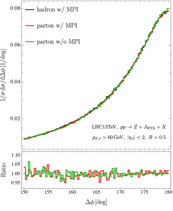
We first examine the sensitivity of the azimuthal decorrelation to hadronization and underlying event in the left panel of figure 10, which shows the $\Delta\phi$ distributions with or without hadronization or underlying event contributions. In Pythia the underlying event is modeled as multi-parton interactions (MPI). We see that the shape of the $\Delta\phi$ distribution is remarkably insensitive to hadronization and MPI, which suggests that it is dominated by perturbative contributions. This is expected: due to our recoil-free jet definition, these soft contributions do not interfere with the jet finding, and only provide a total recoil of the $V+$jet system. Since the azimuthal angle is a vector quantity, the net effect of this recoil tends to be (close to) zero. There is a change in the normalization of the absolute cross section, because the additional radiation affects the number of events having a jet with sufficient transverse momentum.

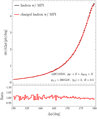
In order to exploit the high angular resolution of charged particle tracking, we study the case where the recoil-free axis is determined only by charged tracks, and the difference compared to using all charged and neutral particles is examined. This is shown in the right panel of figure 10. As can be seen, the azimuthal decorrelation distributions using the recoil-free axis determined by charged particles or all the particles within jets are almost identical, in line with the our conclusion in sec. 4.3 that this difference is beyond NLL accuracy.

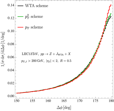
To contrast the WTA axis choice, we provide distributions for jets defined using the more general $p_{t}^{n}$ recombination scheme in eq. (4.2). In the left panel of figure 11 we examine the case where $n=1$ (the standard), $n=2$ and $n\rightarrow\infty$ (WTA). Since the WTA axis is sensitive to momentum-conserving collinear splittings within jets and following the energetic branch, the $\Delta\phi$ distribution is broader near the back-to-back region. The difference between the recoil-free $n=2$ and WTA axis is beyond NLL order, as discussed in sec. 4.2, and is indeed small. The difference with the recoil-sensitive case $n=1$ is larger.

Figure 11: Normalized $\Delta\phi$ distribution for $Z$+jet in Pythia. Left: for WTA, $p_{T}^{2}$ and $p_{T}$ recombination schemes. Right: for WTA with jet radii $R=0.5,0.8$ and $1.0$. Our factorization predicts that the cross section is independent of $R$ if $\delta\phi\ll R$.

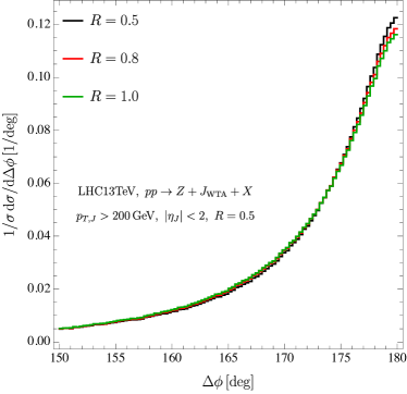
We also compare the distributions for jets with different radii as a way to highlight again the insensitivity to soft, typically wide angle, radiation, in the limit where the jet radii are much larger than the azimuthal decorrelation, $\delta\phi\ll R$. The right panel of figure 11 shows the $\Delta\phi$ distributions for jets reconstructed using different jet radii, namely $R=0.5$, $R=0.8$ and $R=1.0$. The shapes of the distributions are very similar as expected from our factorization analysis. The differences for $\Delta\phi$ in the vicinity of $180^{\circ}$ arise because these distributions are normalized. However, some normalization is necessary when comparing different jet radii, because the jet radius has a non-negligible (5-10%) effect on the normalization of the cross section through the cut on the jet transverse momentum.

6.2 Resummed predictions

In this section we present numerical results from the resummation formula in eq. (5.1), which we match to MCFM Campbell:2002tg ; Campbell:2003hd using the procedure described in sec. 5.2. The electroweak parameters are given by

$$m_{Z}=91.1876~{}{\rm GeV},~{}~{}~{}\alpha_{em}=1/132.34\,,~{}~{}~{}\cos\theta_{W}=0.88168\,,$$ (103)

and we use CT14nlo Dulat:2015mca with $\alpha_{s}(m_{Z})=0.118$ for the collinear PDFs.

Figure 12: The $\delta\phi$ differential distributions at NLO order for jet transverse momentum $p_{T,J}>60\,{\rm GeV}$ (left) and $p_{T,J}>200\,{\rm GeV}$ (right) with jet radius $R=0.5$ (blue), $1.0$ (red) and the $R$-independent singular terms (green). The non-singular cross section (difference of the NLO and NLO singular) is shown in the lower panels.

Figure 13: Diagrams for the $gg\to Zq\bar{q}$ contribution to $Z$+jet production (diagrams where the direction of the quark line is reversed are omitted). Our factorization formula only includes the singular contributions in the expansion of diagrams (a) and (b) around the back-to-back limit of the boson and jet. There are power corrections at $\mathcal{O}(\alpha_{s}(\delta\phi)^{0})$ from expanding diagrams (a) and (c) for the emission of a $Z$-boson off dijets, which are included via matching.

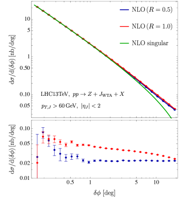
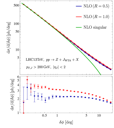
We start in figure 12 with a detailed comparison of our factorization formula in eq. (5.1), expanded at NLO in eq. (5.2), with predictions from MCFM. As confirmed in the upper panels of this figure, the singular terms agree with the NLO for both $p_{T,J}>60$ GeV and $p_{T,J}>200$ GeV. The lower panels of this figure show the importance of the matching procedure at NNLL because of $\mathcal{O}(\alpha_{s}(\delta\phi)^{0})$ power corrections, which are not contained in our factorization formula. More explicitly, our factorization in eq. (5.1) only includes singular $1/(\delta\phi)$ terms from expanding around the back-to-back limit of the boson and jet, missing an important contribution to the power corrections that arises from a dijet configuration where a $Z$ boson is emitted from one of the jets. This contribution enters at the same order in the coupling and is enhanced for $p_{T,J}\ll m_{Z}$, as will be discussed below. To illustrate the difference between the contributions in the factorization theorem and this important nonsingular correction, consider the diagrams for the $gg\to q\bar{q}Z$ process in figure 13: Diagrams (a) and (b) contribute to our factorization theorem in the region of phase-space where a final-state quark is collinear to one of the incoming gluons. However, diagram (a) and the new diagram (c) are also enhanced for the region of phase space describing a $Z$ emission of a dijet configuration. This contribution is included by the matching procedure in sec. 5.2 and discussed more below.

Figure 14: The distribution in the azimuthal angle $\Delta\phi_{12}$ between the two final-state partons at NLO. For $p_{T,J}\lesssim m_{V}$ there is a collinear singularity at $\Delta\phi_{12}\to 0$, while for $p_{T,J}\gg m_{V}$ there is also a collinear singularity at $\Delta\phi_{12}\to 180^{\circ}$ from a $Z$ boson emitted from a dijet partonic configuration.

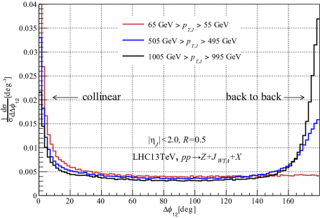
For $p_{T,J}\ll m_{V}$, the order $\alpha_{s}(\delta\phi)^{0}$ power corrections from the $Z$ emission off dijets are power suppressed in $m_{V}$. This can be seen by expanding the diagrams in figure 13 describing soft-collinear corrections around the back-to-back limit, yielding contributions proportional to $\frac{1}{m_{V}^{2}}\frac{1}{(\delta\phi)^{2}p_{T,V}^{2}}$ at the amplitude level, while the $Z$ emission of dijets is proportional to $\frac{1}{m_{V}^{4}}$. Accordingly, at low $p_{T}$, the $Z$ emission off dijets is expected to be independent of the azimuthal angle based on the above expansion. Indeed, the non-singular in figure 12 is almost constant at small $\delta\phi$. This is also confirmed by looking at the azimuthal angle $\Delta\phi_{12}$ of the two final-state partons shown in figure 14. We find that for $p_{T,J}\lesssim m_{V}$ (e.g. the 65 GeV$>p_{T,J}>55$ GeV bin) the $\Delta\phi_{12}$ distribution is flat near $\Delta\phi_{12}=180^{\circ}$. This flatness is the reason that we do not expect the nonsingular to go to zero at $\Delta\phi\to 180^{\circ}$, and don’t employ a multiplicative matching that would enforce that. Indeed, collinear and soft emissions will smear the nonsingular $\delta\phi$ distribution, but since it is (almost) constant it will not change (much).

Figure 14 also shows that at high $p_{T,J}$ there are large contributions from the $Z$ emission off back-to-back dijets, in addition to soft-collinear QCD radiation for back-to-back boson-jet production. The latter is the focus of this paper, incorporated in the resummation formula eq. (5.1), while the former is included by matching and needed at NNLL and beyond. When $p_{T,J}\gg m_{V}$, it is insufficient to include this contribution by matching in the region $m_{V}/p_{T,J}\lesssim\delta\phi\ll 1$, as it now also contains large logarithms of $\delta\phi$ that require resummation. Alternatively, one can also remove the contribution of a $Z$ boson emitted from a dijet by introducing an isolation cone around the boson (or its decay products).

Figure 15: Our resummed predictions (blue) matched to NLO (green) for the $Z$+jet azimuthal decorrelation $\Delta\phi$ for $p_{T,J}>60$ GeV (left) and $p_{T,J}>200$ GeV (right). Our predictions are compared to Pythia simulations at the hadron level with MPI contributions (black) and the NLO (red). The band represents the perturbative uncertainty, which is estimated by scale variation (see sec. 5.1). The larger nonsingular corrections (from the matching) are discussed in the text.

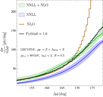
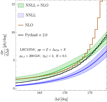
We conclude by showing in figure 15 our resummed predictions at NNLL+NLO accuracy, and comparing to Pythia results at hadron level with MPI contributions for the two $p_{T,J}$ regions. We show the resummed predictions with and without matching, in view of the large power corrections we just discussed, and also include the NLO cross section as a separate curve. The NLO cross section divergences as $\Delta\phi\to 180^{\circ}$, which is remedied by the resummation. Our resummed results without matching agree with the shape of Pythia simulations. By including the matching, our predictions smoothly approach NLO for smaller values of $\Delta\phi$, where resummation is not needed. The large nonsingular correction (larger than our uncertainty bands) is important to include and cannot be neglected as $\Delta\phi\to 180^{\circ}$. It is not accounted for in the Pythia simulations we used. Simply attempting to include it through a $K$-factor does not yield the correct shape, particularly at high $p_{T,J}$.

7 Conclusions

In this paper we describe our calculation of the cross section for a vector boson and jet, differential in the azimuthal decorrelation $\delta\phi$, at next-to-next-to-leading logarithmic order. We provide substantially more details than our earlier work Chien:2020hzh , an expanded phenomenological analysis, and also include a Pythia study. We discuss for the first time why the azimuthal angle is simpler than the total transverse momentum $\vec{q}_{T}$, potential Glauber contributions, different recoil-free recombination schemes, the jet radius dependence, and the non-singular matching.

Our focus is on the region $\delta\phi\ll 1$, which dominates the cross section and requires the resummation of logarithms of $\delta\phi$ to obtain reliable predictions. We carried out a detailed study of its factorization in SCET, deriving a factorization formula. We investigated potential factorization-violating Glauber contributions, finding that they could first appear at order $\alpha_{s}^{4}$. Many of the ingredients in the factorization are available, and we present calculations of the jet functions, including the linearly polarized jet function, as well as jet functions for $p_{T}^{n}$-weighted recombination schemes. We find that these different recombination schemes only change the constant term in the jet function, having a minimal effect on the prediction. Furthermore, we verify the independence on the jet radius predicted by the factorization (for $R\gg\delta\phi$) in Pythia. By using the (rapidity) renormalization group we achieve the resummation of logarithms of $\delta\phi$.

The key to obtaining predictions beyond NLL is a recoil-free recombination scheme, which reduces the effect of soft radiation to a total recoil of the $V+$jet system, eliminating non-global logarithms. This is in contrast to the standard recombination scheme, or other transverse momentum measurements such as the radial decorrelation, which involve NGLs. A recoil-free recombination scheme is also interesting for studying the properties of the medium in heavy-ion collisions, because it is more sensitive to collinear splittings inside the jet and less sensitive to contamination of soft radiation. Indeed, we observe negligible effects of hadronization and MPI contributions in Pythia, as well as compatibility with track-based measurements. Our resummed predictions are matched to MCFM in the region where $\delta\phi$ is no longer small. Here we find that the non-singular contributions are quite large, particularly for high jet $p_{T}$, increasing the sensitivity to the details of the matching procedure. It would be interesting to investigate the resummation of these power corrections.

We have established the azimuthal angle between a vector boson and a recoil-free jet, as a robust observable for which high precision is possible. In this paper we achieve NNLL order, but NNNLL is within reach. As the effect of the underlying event, hadronization and from performing the measurement using charged particle tracks is minimal, it is attractive experimentally.

Appendix A Anomalous dimensions

In general, for the (next-to)ⁱ -leading logarithmic (NⁱLL) resummation, one needs up to $(i-1)$-loop fixed-order ingredients, $i$-loop non-cusp anomalous dimensions and the $(i+1)$-loop cusp anomalous dimension and QCD beta function. In this appendix, we collect the beta function and all the anomalous dimensions that are needed for this paper.

For the beta function,

$$\frac{\mathrm{d}\alpha_{s}(\mu)}{\mathrm{d}\ln\mu}=-2\varepsilon\alpha_{s}+\beta(\alpha_{s}),~{}~{}~{}\beta(\alpha_{s})=-2\alpha_{s}\sum_{n=0}^{\infty}\beta_{n}\left(\frac{\alpha_{s}}{4\pi}\right)^{n+1}$$ (104)

one has up to three loops Tarasov:1980au ; Larin:1993tp

$$\beta_{0} =\frac{11}{3}C_{A}-\frac{4}{3}T_{F}n_{f}\,,$$

$$\beta_{1} =\frac{34}{3}C_{A}^{2}-\frac{20}{3}C_{A}T_{F}n_{f}-4C_{F}T_{F}n_{f}\,,$$

$$\beta_{2} =\frac{2857}{54}C_{A}^{3}+\left(2C_{F}^{2}-\frac{205}{9}C_{F}C_{A}-\frac{1415}{27}C_{A}^{2}\right)T_{F}n_{f}+\left(\frac{44}{9}C_{F}+\frac{158}{27}C_{A}\right)T_{F}^{2}n_{f}^{2}\,,$$ (105)

where $n_{f}$ is the number of active quark flavors.

Identifying standard anomalous dimensions by their associated functions, and using the universality of the rapidity anomalous dimension, we write the perturbative expansions of cusp, non-cusp, and rapidity anomalous dimensions as

$$\Gamma_{\rm cusp}=\sum\limits_{n=0}^{\infty}\left(\frac{\alpha_{s}}{4\pi}\right)^{n+1}\Gamma_{n}\,,\quad\gamma_{\mu}^{i}=\sum\limits_{n=0}^{\infty}\left(\frac{\alpha_{s}}{4\pi}\right)^{n+1}\gamma^{i}_{n}\,,\quad\gamma_{\nu}=\sum\limits_{n=0}^{\infty}\left(\frac{\alpha_{s}}{4\pi}\right)^{n+1}\gamma^{\nu}_{n}.$$ (106)

The cusp anomalous dimension is, up to three loops, given by Korchemsky:1987wg ; Moch:2004pa

$$\Gamma_{0} =4\,,$$

$$\Gamma_{1} =\left(\frac{268}{9}-\frac{4\pi^{2}}{3}\right)C_{A}-\frac{80}{9}\,T_{F}n_{f}\,,$$

$$\Gamma_{2} =C_{A}^{2}\left(\frac{490}{3}-\frac{536\pi^{2}}{27}+\frac{44\pi^{4}}{45}+\frac{88}{3}\,\zeta_{3}\right)+C_{A}T_{F}n_{f}\left(-\frac{1672}{27}+\frac{160\pi^{2}}{27}-\frac{224}{3}\,\zeta_{3}\right)$$

$$\quad+C_{F}T_{F}n_{f}\left(-\frac{220}{3}+64\zeta_{3}\right)-\frac{64}{27}\,T_{F}^{2}n_{f}^{2}\,.$$ (107)

The non-cusp anomalous dimension for the hard function can be extracted Idilbi:2006dg ; Becher:2006mr ; Becher:2009qa from the massless quark and gluon form factor, which are known at three loop order Moch:2005tm . They are given by

$$\gamma_{0}^{q} =-3C_{F}\,,$$

$$\gamma_{1}^{q} =C_{F}^{2}\left(-\frac{3}{2}+2\pi^{2}-24\zeta_{3}\right)+C_{F}C_{A}\left(-\frac{961}{54}-\frac{11\pi^{2}}{6}+26\zeta_{3}\right)+C_{F}T_{F}n_{f}\left(\frac{130}{27}+\frac{2\pi^{2}}{3}\right),$$

$$\gamma_{0}^{g} =-\beta_{0}=-\frac{11}{3}\,C_{A}+\frac{4}{3}\,T_{F}n_{f}\,,$$

$$\gamma_{1}^{g} =C_{A}^{2}\left(-\frac{692}{27}+\frac{11\pi^{2}}{18}+2\zeta_{3}\right)+C_{A}T_{F}n_{f}\left(\frac{256}{27}-\frac{2\pi^{2}}{9}\right)+4C_{F}T_{F}n_{f}\,,$$ (108)

for gluons. The non-cusp anomalous dimensions for the beam and soft functions are given by Luebbert:2016itl

$$\gamma_{0}^{B_{q}} =6C_{F}\,,$$

$$\gamma_{1}^{B_{q}} =C_{F}^{2}\left(3-4\pi^{2}+48\zeta_{3}\right)+C_{F}C_{A}\left(\frac{17}{3}+\frac{44\pi^{2}}{9}-24\zeta_{3}\right)+C_{F}T_{F}n_{f}\left(-\frac{4}{3}-\frac{16\pi^{2}}{9}\right)\,,$$

$$\gamma_{0}^{B_{g}} =2\beta_{0}\,,$$

$$\gamma_{1}^{B_{g}} =C_{A}^{2}\left(\frac{64}{3}+24\zeta_{3}\right)-\frac{32}{3}C_{A}T_{F}n_{f}-8C_{F}T_{F}n_{f}\,,$$ (109)

$$\gamma_{0}^{S} =0\,,\qquad\gamma_{1}^{S}=C_{A}\left(\frac{64}{9}-28\,\zeta_{3}\right)+\beta_{0}\left(\frac{56}{9}-\frac{\pi^{2}}{3}\right)\,.$$ (110)

Finally, the non-cusp rapidity anomalous dimension is given by Gehrmann:2012ze ; Gehrmann:2014yya ; Echevarria:2015byo ; Luebbert:2016itl

$$\gamma_{0}^{\nu}=0\,,\qquad\gamma_{1}^{\nu}=-C_{A}\left(\frac{128}{9}-56\,\zeta_{3}\right)-\beta_{0}\frac{112}{9}\,.$$ (111)

The most convenient choice of scales in our problem is $\mu=\mu_{J}=\mu_{S}=\mu_{B}$ and $\nu=\mu_{B}$. With this choice, the simplest path to solve the RG equations, eq. (84), is shown in figure 5. With $\mu=\mu_{B}$ fixed, the beam and jet functions run from their natural rapidity scales $\nu_{i}$ down to $\nu=\mu_{B}$, the natural rapidity scale of the soft function. Only the hard function is required to run in $\mu$ from $\mu_{H}$ to $\mu_{B}$. Generically, the hard anomalous dimension takes the form

$$\Gamma(\alpha_{s})=C_{\Gamma}\Gamma_{\text{cusp}}(\alpha_{s})\ln\frac{Q_{\Gamma}^{2}}{\mu^{2}}+\gamma(\alpha_{s}).$$ (112)

The corresponding ordinary RG running boils down to the evaluation of the following functions:

$$S(\mu_{H},\mu)=\int_{\mu_{H}}^{\mu}\frac{\mathrm{d}\bar{\mu}}{\bar{\mu}}\ln\frac{\mu_{H}}{\bar{\mu}}\Gamma_{\rm cusp}(\alpha_{s}(\bar{\mu})),\qquad A_{\gamma^{i}}(\mu_{H},\mu)=-\int_{\mu_{H}}^{\mu}\frac{\mathrm{d}\bar{\mu}}{\bar{\mu}}\gamma^{i}(\alpha_{s}(\bar{\mu})).$$ (113)

In terms of these two functions, one has

$$e^{\int_{\mu_{H}}^{\mu}\frac{\mathrm{d}\bar{\mu}}{\bar{\mu}}\Gamma(\bar{\mu})}=\left(\frac{Q_{\Gamma}^{2}}{\mu_{H}^{2}}\right)^{-C_{\Gamma}A_{\gamma_{\text{cusp}}}(\mu_{H},\mu)}e^{2C_{\Gamma}S(\mu_{H},\mu)-2A_{\gamma}(\mu_{H},\mu)}.$$ (114)

At NNLL, we only keep terms up to $O(\alpha_{s})$, that is

$$A_{\gamma^{\text{i}}}(\mu_{H},\mu) =-\int_{\alpha_{s}(\mu_{H})}^{\alpha_{s}(\mu)}\frac{\mathrm{d}\alpha}{\beta(\alpha)}\gamma^{\text{i}}(\alpha)$$

$$=\frac{1}{2}\frac{\gamma_{0}^{\text{i}}}{\beta_{0}}\int_{\alpha_{s}(\mu_{H})}^{\alpha_{s}(\mu)}\frac{\mathrm{d}\alpha}{\alpha}\frac{1+\sum\limits_{l=1}^{\infty}\left(\frac{\alpha}{4\pi}\right)^{l}\frac{\gamma_{l}^{\text{i}}}{\gamma_{l}^{\text{0}}}}{1+\sum\limits_{l=1}^{\infty}\left(\frac{\alpha}{4\pi}\right)^{l}\frac{\beta_{l}}{\beta_{0}}}$$

$$=\frac{1}{2}\frac{\gamma_{0}^{\text{i}}}{\beta_{0}}\left[\ln r+\frac{\alpha_{s}(\mu_{H})}{4\pi}\Big{(}\frac{\beta_{1}}{\beta_{0}}-\frac{\gamma_{1}^{i}}{\gamma_{0}^{i}}\Big{)}(1-r)\right]$$ (115)

and

$$S(\mu_{H},\mu)=-\int_{\alpha_{s}(\mu_{H})}^{\alpha_{s}(\mu)} \frac{\mathrm{d}\bar{\alpha}}{\beta(\bar{\alpha})}\Gamma_{\rm cusp}(\bar{\alpha})\int^{\bar{\alpha}}_{\alpha_{s}(\mu_{H})}\frac{\mathrm{d}\alpha}{\beta(\alpha)}$$

$$=\frac{\Gamma_{0}}{4\beta_{0}^{2}}\bigg{\{} \frac{4\pi}{\alpha_{s}(\mu_{H})}\bigg{(}\frac{r-1}{r}-\log r\bigg{)}$$

$$+\Big{(}\frac{\beta_{1}}{\beta_{0}}-\frac{\Gamma_{1}}{\Gamma_{0}}\Big{)}(r-1-\log r)+\frac{\beta_{1}}{2\beta_{0}}\log^{2}r$$

$$-\frac{\alpha_{s}(\mu_{H})}{8\pi}\bigg{[}\frac{\Gamma_{2}}{\Gamma_{0}}(r-1)^{2}+\frac{\beta_{2}}{\beta_{0}}(1-r^{2}+2\log r)+\frac{\beta_{1}^{2}}{\beta_{0}^{2}}(r-1)$$

$$\times(r-1+2\log r)-\frac{\beta_{1}}{\beta_{0}}\frac{\Gamma_{1}}{\Gamma_{0}}(r^{2}-4r+2r\log r+3)\bigg{]}\bigg{\}}$$ (116)

with

$$r\equiv\frac{\alpha_{s}(\mu)}{\alpha_{s}(\mu_{H})}.$$ (117)

Appendix B One-loop hard function

In this appendix we give the expressions of the one-loop hard function. Since we do not need the one-loop hard function for a linearly-polarized gluon at NNLL accuracy, we only give the results for an unpolarized gluon here. After factorizing the LO hard function, the one-loop hard function has the form as

$$\mathcal{H}^{(1)}_{ij\to Vk}=\mathcal{H}^{(0)}_{ij\to Vk}C_{ij\to Vk}(\hat{t},\hat{u}).$$ (118)

For the $q\bar{q}\to Vg$ channel, we have

$$C_{q\bar{q}\to Vg}(t,u) =C_{A}\frac{\pi^{2}}{6}+C_{F}\left(-16+\frac{7\pi^{2}}{3}\right)+2C_{A}\ln^{2}\frac{s}{m_{V}^{2}}+C_{A}\ln^{2}\frac{m_{V}^{2}-t}{m_{V}^{2}}$$

$$+C_{A}\ln^{2}\frac{m_{V}^{2}-u}{m_{V}^{2}}+\ln\frac{s}{m_{V}^{2}}\left(-6C_{F}-2C_{A}\ln\frac{s^{2}}{tu}\right)-C_{A}\ln^{2}\frac{tu}{m_{V}^{4}}-6C_{F}\ln\frac{\mu^{2}}{s}$$

$$-2C_{A}\ln\frac{s^{2}}{tu}\ln\frac{\mu^{2}}{s}+\left(-C_{A}-2C_{F}\right)\ln^{2}\frac{\mu^{2}}{s}$$

$$+2C_{A}\operatorname{Li}_{2}\left(\frac{m_{V}^{2}}{m_{V}^{2}-t}\right)+2C_{A}\operatorname{Li}_{2}\left(\frac{m_{V}^{2}}{m_{V}^{2}-u}\right)$$

$$+\frac{2}{T_{0}(u,t)}\left\{C_{F}\left(\frac{s}{s+t}+\frac{s+t}{u}+\frac{s}{s+u}+\frac{s+u}{t}\right)\right.$$

$$+\left(-C_{A}+2C_{F}\right)\left[-\frac{m_{V}^{2}\left(t^{2}+u^{2}\right)}{tu(t+u)}+2\left(\frac{s^{2}}{(t+u)^{2}}+\frac{2s}{t+u}\right)\ln\frac{s}{m_{V}^{2}}\right]$$

$$+\left(C_{A}\frac{t}{s+u}+C_{F}\frac{4s^{2}+2st+4su+tu}{(s+u)^{2}}\right)\ln\frac{-t}{m_{V}^{2}}$$

$$+\left(C_{A}\frac{u}{s+t}+C_{F}\frac{4s^{2}+4st+2su+tu}{(s+t)^{2}}\right)\ln\frac{-u}{m_{V}^{2}}$$

$$-\left(-C_{A}+2C_{F}\right)\left[\frac{s^{2}+(s+u)^{2}}{tu}\left(\frac{1}{2}\ln^{2}\frac{s}{m_{V}^{2}}-\frac{1}{2}\ln^{2}\frac{m_{V}^{2}-t}{m_{V}^{2}}+\ln\frac{s}{m_{V}^{2}}\ln\frac{-t}{s-m_{V}^{2}}\right.\right.$$

$$\left.+\operatorname{Li}_{2}\left(\frac{m_{V}^{2}}{s}\right)-\operatorname{Li}_{2}\left(\frac{m_{V}^{2}}{m_{V}^{2}-t}\right)\right)$$

$$+\frac{s^{2}+(s+t)^{2}}{tu}\left(\frac{1}{2}\ln^{2}\frac{s}{m_{V}^{2}}-\frac{1}{2}\ln^{2}\frac{m_{V}^{2}-u}{m_{V}^{2}}+\ln\frac{s}{m_{V}^{2}}\ln\frac{-u}{s-m_{V}^{2}}\right.$$

$$\left.\left.+\operatorname{Li}_{2}\left(\frac{m_{V}^{2}}{s}\right)-\operatorname{Li}_{2}\left(\frac{m_{V}^{2}}{m_{V}^{2}-u}\right)\right)\right],$$ (119)

and for the $qg\to Vq$ channel we have

$$C_{qg\to Vq}(t,u) =C_{A}\frac{7\pi^{2}}{6}+C_{F}\left(-16+\frac{\pi^{2}}{3}\right)-6C_{F}\ln\frac{s}{m_{V}^{2}}-C_{A}\ln^{2}\frac{-st}{m_{V}^{4}}+C_{A}\ln^{2}\frac{m_{V}^{2}-t}{m_{V}^{2}}$$

$$+2C_{A}\ln\frac{\left(s-m_{V}^{2}\right)t}{m_{V}^{2}u}\ln\frac{-u}{m_{V}^{2}}+C_{A}\ln^{2}\frac{-u}{m_{V}^{2}}-2C_{A}\ln\frac{\left(m_{V}^{2}-s\right)st}{m_{V}^{2}u^{2}}\ln\frac{-u}{s}$$

$$-2C_{A}\ln^{2}\frac{-u}{s}-2C_{F}\ln^{2}\frac{-u}{s}+\left(-6C_{F}+2C_{A}\ln\frac{t}{u}+4C_{F}\ln\frac{-u}{s}\right)\ln\frac{\mu^{2}}{s}$$

$$-\left(C_{A}+2C_{F}\right)\ln^{2}\frac{\mu^{2}}{s}-2C_{A}\operatorname{Li}_{2}\left(\frac{m_{V}^{2}}{s}\right)+2C_{A}\operatorname{Li}_{2}\left(\frac{m_{V}^{2}}{m_{V}^{2}-t}\right)$$

$$+\frac{2}{T_{0}(s,t)}\left\{C_{F}\left(\frac{u}{s+u}+\frac{s+u}{t}+\frac{u}{t+u}+\frac{t+u}{s}\right)\right.$$

$$+\left(C_{A}\frac{s}{t+u}+C_{F}\frac{st+2su+4tu+4u^{2}}{(t+u)^{2}}\right)\ln\frac{s}{m_{V}^{2}}$$

$$+\left(C_{A}\frac{t}{s+u}+C_{F}\frac{st+4su+2tu+4u^{2}}{(s+u)^{2}}\right)\ln\frac{-t}{m_{V}^{2}}$$

$$+\left(-C_{A}+2C_{F}\right)\left[-\frac{m_{V}^{2}\left(s^{2}+t^{2}\right)}{st(s+t)}+2\left(\frac{2u}{s+t}+\frac{u^{2}}{(s+t)^{2}}\right)\ln\frac{-u}{m_{V}^{2}}\right]$$

$$-\left(-C_{A}+2C_{F}\right)\left[\frac{u^{2}+(t+u)^{2}}{st}\left(\frac{1}{2}\ln^{2}\frac{s}{m_{V}^{2}}-\frac{1}{2}\ln^{2}\frac{m_{V}^{2}-u}{m_{V}^{2}}+\ln\frac{s}{m_{V}^{2}}\ln\frac{-u}{s-m_{V}^{2}}\right.\right.$$

$$\left.+\mathrm{Li}_{2}\left(\frac{m_{V}^{2}}{s}\right)-\mathrm{Li}_{2}\left(\frac{m_{V}^{2}}{m_{V}^{2}-u}\right)\right)$$

$$+\frac{u^{2}+(s+u)^{2}}{st}\left(-\frac{\pi^{2}}{2}-\frac{1}{2}\ln^{2}\frac{m_{V}^{2}-t}{m_{V}^{2}}-\frac{1}{2}\ln^{2}\frac{m_{V}^{2}-u}{m_{V}^{2}}+\ln\frac{-t}{m_{V}^{2}}\ln\frac{-u}{m_{V}^{2}}\right.$$

$$\left.\left.\left.-\mathrm{Li}_{2}\left(\frac{m_{V}^{2}}{m_{V}^{2}-t}\right)-\operatorname{Li}_{2}\left(\frac{m_{V}^{2}}{m_{V}^{2}-u}\right)\right)\right]\right\},$$ (120)

with the function $T_{0}$ defined as

$$T_{0}(u,t)=\frac{u}{t}+\frac{t}{u}+\frac{2m_{V}^{2}\left(m_{V}^{2}-t-u\right)}{tu}.$$ (121)

References

- (1) CMS collaboration, Event Shapes and Azimuthal Correlations in + Jets Events in Collisions at TeV, Phys. Lett. B722 (2013) 238 [1301.1646].
- (2) CMS collaboration, Measurement of the Triple-Differential Cross Section for Photon+Jets Production in Proton-Proton Collisions at =7 TeV, JHEP 06 (2014) 009 [1311.6141].
- (3) ATLAS collaboration, High- isolated-photon plus jets production in collisions at 8 TeV with the ATLAS detector, Nucl. Phys. B 918 (2017) 257 [1611.06586].
- (4) CMS collaboration, Measurements of differential production cross sections for a Z boson in association with jets in pp collisions at TeV, JHEP 04 (2017) 022 [1611.03844].
- (5) CMS collaboration, Study of Jet Quenching with Correlations in Pb-Pb and Collisions at , Phys. Rev. Lett. 119 (2017) 082301 [1702.01060].
- (6) ATLAS collaboration, Measurement of the cross section for isolated-photon plus jet production in collisions at TeV using the ATLAS detector, Phys. Lett. B780 (2018) 578 [1801.00112].
- (7) CMS collaboration, Study of jet quenching with isolated-photon+jet correlations in PbPb and pp collisions at 5.02 TeV, Phys. Lett. B 785 (2018) 14 [1711.09738].
- (8) V. Kartvelishvili, R. Kvatadze and R. Shanidze, On Z and Z + jet production in heavy ion collisions, Phys. Lett. B 356 (1995) 589 [hep-ph/9505418].
- (9) X. Chen, T. Gehrmann, E. W. N. Glover and M. Jaquier, Precise QCD predictions for the production of Higgs + jet final states, Phys. Lett. B 740 (2015) 147 [1408.5325].
- (10) A. Gehrmann-De Ridder, T. Gehrmann, E. W. N. Glover, A. Huss and T. A. Morgan, Precise QCD predictions for the production of a Z boson in association with a hadronic jet, Phys. Rev. Lett. 117 (2016) 022001 [1507.02850].
- (11) R. Boughezal, C. Focke, X. Liu and F. Petriello, -boson production in association with a jet at next-to-next-to-leading order in perturbative QCD, Phys. Rev. Lett. 115 (2015) 062002 [1504.02131].
- (12) R. Boughezal, J. M. Campbell, R. K. Ellis, C. Focke, W. T. Giele, X. Liu et al., Z-boson production in association with a jet at next-to-next-to-leading order in perturbative QCD, Phys. Rev. Lett. 116 (2016) 152001 [1512.01291].
- (13) R. Boughezal, F. Caola, K. Melnikov, F. Petriello and M. Schulze, Higgs boson production in association with a jet at next-to-next-to-leading order, Phys. Rev. Lett. 115 (2015) 082003 [1504.07922].
- (14) R. Boughezal, C. Focke, W. Giele, X. Liu and F. Petriello, Higgs boson production in association with a jet at NNLO using jettiness subtraction, Phys. Lett. B 748 (2015) 5 [1505.03893].
- (15) J. M. Campbell, R. K. Ellis and C. Williams, Direct Photon Production at Next-to–Next-to-Leading Order, Phys. Rev. Lett. 118 (2017) 222001 [1612.04333].
- (16) A. Gehrmann-De Ridder, T. Gehrmann, E. W. N. Glover, A. Huss and D. M. Walker, Next-to-Next-to-Leading-Order QCD Corrections to the Transverse Momentum Distribution of Weak Gauge Bosons, Phys. Rev. Lett. 120 (2018) 122001 [1712.07543].
- (17) X. Chen, T. Gehrmann, N. Glover, M. Höfer and A. Huss, Isolated photon and photon+jet production at NNLO QCD accuracy, JHEP 04 (2020) 166 [1904.01044].
- (18) A. Gehrmann-De Ridder, T. Gehrmann, E. W. N. Glover, A. Huss and D. M. Walker, Vector Boson Production in Association with a Jet at Forward Rapidities, Eur. Phys. J. C 79 (2019) 526 [1901.11041].
- (19) M. Czakon, A. Mitov, M. Pellen and R. Poncelet, NNLO QCD predictions for W+c-jet production at the LHC, JHEP 06 (2021) 100 [2011.01011].
- (20) R. Mondini and C. Williams, Bottom-induced contributions to Higgs plus jet at next-to-next-to-leading order, JHEP 05 (2021) 045 [2102.05487].
- (21) R. Gauld, A. Gehrmann-De Ridder, T. Gehrmann, E. W. N. Glover, A. Huss, I. Majer et al., Transverse momentum distributions in low-mass Drell-Yan lepton pair production at NNLO QCD, 2110.15839.
- (22) A. Banfi, M. Dasgupta and Y. Delenda, Azimuthal decorrelations between QCD jets at all orders, Phys. Lett. B665 (2008) 86 [0804.3786].
- (23) L. Chen, G.-Y. Qin, L. Wang, S.-Y. Wei, B.-W. Xiao, H.-Z. Zhang et al., Study of Isolated-photon and Jet Momentum Imbalance in and collisions, Nucl. Phys. B 933 (2018) 306 [1803.10533].
- (24) P. Sun, B. Yan, C. P. Yuan and F. Yuan, Resummation of High Order Corrections in Boson Plus Jet Production at the LHC, Phys. Rev. D 100 (2019) 054032 [1810.03804].
- (25) Y.-T. Chien, D. Y. Shao and B. Wu, Resummation of Boson-Jet Correlation at Hadron Colliders, JHEP 11 (2019) 025 [1905.01335].
- (26) L. Buonocore, M. Grazzini, J. Haag and L. Rottoli, Transverse-momentum resummation for boson plus jet production at hadron colliders, 2110.06913.
- (27) Y. Hatta, B.-W. Xiao, F. Yuan and J. Zhou, Azimuthal angular asymmetry of soft gluon radiation in jet production, Phys. Rev. D 104 (2021) 054037 [2106.05307].
- (28) S. Cao and X.-N. Wang, Jet quenching and medium response in high-energy heavy-ion collisions: a review, Rept. Prog. Phys. 84 (2021) 024301 [2002.04028].
- (29) M. Dasgupta and G. P. Salam, Resummation of nonglobal QCD observables, Phys. Lett. B 512 (2001) 323 [hep-ph/0104277].
- (30) Y.-T. Chien, R. Rahn, S. Schrijnder van Velzen, D. Y. Shao, W. J. Waalewijn and B. Wu, Recoil-free azimuthal angle for precision boson-jet correlation, Phys. Lett. B 815 (2021) 136124 [2005.12279].
- (31) H.-M. Chang, M. Procura, J. Thaler and W. J. Waalewijn, Calculating Track-Based Observables for the LHC, Phys. Rev. Lett. 111 (2013) 102002 [1303.6637].
- (32) H.-M. Chang, M. Procura, J. Thaler and W. J. Waalewijn, Calculating Track Thrust with Track Functions, Phys. Rev. D 88 (2013) 034030 [1306.6630].
- (33) G. Salam, “ Scheme.” Unpublished.
- (34) D. Bertolini, T. Chan and J. Thaler, Jet Observables Without Jet Algorithms, JHEP 04 (2014) 013 [1310.7584].
- (35) C. W. Bauer, S. Fleming, D. Pirjol and I. W. Stewart, An Effective field theory for collinear and soft gluons: Heavy to light decays, Phys. Rev. D63 (2001) 114020 [hep-ph/0011336].
- (36) C. W. Bauer and I. W. Stewart, Invariant operators in collinear effective theory, Phys. Lett. B516 (2001) 134 [hep-ph/0107001].
- (37) C. W. Bauer, D. Pirjol and I. W. Stewart, Soft collinear factorization in effective field theory, Phys. Rev. D65 (2002) 054022 [hep-ph/0109045].
- (38) C. W. Bauer, S. Fleming, D. Pirjol, I. Z. Rothstein and I. W. Stewart, Hard scattering factorization from effective field theory, Phys. Rev. D66 (2002) 014017 [hep-ph/0202088].
- (39) M. Beneke, A. P. Chapovsky, M. Diehl and T. Feldmann, Soft collinear effective theory and heavy to light currents beyond leading power, Nucl. Phys. B643 (2002) 431 [hep-ph/0206152].
- (40) A. J. Larkoski, D. Neill and J. Thaler, Jet Shapes with the Broadening Axis, JHEP 04 (2014) 017 [1401.2158].
- (41) M. Cacciari, G. P. Salam and G. Soyez, FastJet User Manual, Eur. Phys. J. C 72 (2012) 1896 [1111.6097].
- (42) M. Procura, W. J. Waalewijn and L. Zeune, Resummation of Double-Differential Cross Sections and Fully-Unintegrated Parton Distribution Functions, JHEP 02 (2015) 117 [1410.6483].
- (43) A. Banfi, G. Marchesini and G. Smye, Away from jet energy flow, JHEP 08 (2002) 006 [hep-ph/0206076].
- (44) H. Weigert, Nonglobal jet evolution at finite N(c), Nucl. Phys. B 685 (2004) 321 [hep-ph/0312050].
- (45) E. Avsar, Y. Hatta and T. Matsuo, Soft gluons away from jets: Distribution and correlation, JHEP 06 (2009) 011 [0903.4285].
- (46) Y. Hatta and T. Ueda, Resummation of non-global logarithms at finite , Nucl. Phys. B874 (2013) 808 [1304.6930].
- (47) K. Khelifa-Kerfa and Y. Delenda, Non-global logarithms at finite Nc beyond leading order, JHEP 03 (2015) 094 [1501.00475].
- (48) S. Caron-Huot, Resummation of non-global logarithms and the BFKL equation, JHEP 03 (2018) 036 [1501.03754].
- (49) T. Becher, M. Neubert, L. Rothen and D. Y. Shao, Effective Field Theory for Jet Processes, Phys. Rev. Lett. 116 (2016) 192001 [1508.06645].
- (50) A. J. Larkoski, I. Moult and D. Neill, Non-Global Logarithms, Factorization, and the Soft Substructure of Jets, JHEP 09 (2015) 143 [1501.04596].
- (51) R. Ángeles Martínez, M. De Angelis, J. R. Forshaw, S. Plätzer and M. H. Seymour, Soft gluon evolution and non-global logarithms, JHEP 05 (2018) 044 [1802.08531].
- (52) A. Banfi, F. A. Dreyer and P. F. Monni, Next-to-leading non-global logarithms in QCD, JHEP 10 (2021) 006 [2104.06416].
- (53) I. W. Stewart, Lectures on the Soft-Collinear Effective Theory, MIT Open Course Ware, Effective Field Theory (Spring 2013) .
- (54) T. Becher, A. Broggio and A. Ferroglia, Introduction to Soft-Collinear Effective Theory, vol. 896. Springer, 2015, 10.1007/978-3-319-14848-9, [1410.1892].
- (55) T. Becher and M. D. Schwartz, Direct photon production with effective field theory, JHEP 02 (2010) 040 [0911.0681].
- (56) P. Mulders and J. Rodrigues, Transverse momentum dependence in gluon distribution and fragmentation functions, Phys. Rev. D 63 (2001) 094021 [hep-ph/0009343].
- (57) P. M. Nadolsky, C. Balazs, E. L. Berger and C. P. Yuan, Gluon-gluon contributions to the production of continuum diphoton pairs at hadron colliders, Phys. Rev. D 76 (2007) 013008 [hep-ph/0702003].
- (58) S. Mantry and F. Petriello, Factorization and Resummation of Higgs Boson Differential Distributions in Soft-Collinear Effective Theory, Phys. Rev. D81 (2010) 093007 [0911.4135].
- (59) S. Catani and M. Grazzini, QCD transverse-momentum resummation in gluon fusion processes, Nucl. Phys. B845 (2011) 297 [1011.3918].
- (60) T. Becher, M. Neubert and D. Wilhelm, Higgs-Boson Production at Small Transverse Momentum, JHEP 05 (2013) 110 [1212.2621].
- (61) J.-y. Chiu, A. Jain, D. Neill and I. Z. Rothstein, The Rapidity Renormalization Group, Phys. Rev. Lett. 108 (2012) 151601 [1104.0881].
- (62) J.-Y. Chiu, A. Jain, D. Neill and I. Z. Rothstein, A Formalism for the Systematic Treatment of Rapidity Logarithms in Quantum Field Theory, JHEP 05 (2012) 084 [1202.0814].
- (63) J. C. Collins and D. E. Soper, Parton Distribution and Decay Functions, Nucl. Phys. B194 (1982) 445.
- (64) J. C. Collins, D. E. Soper and G. F. Sterman, Transverse Momentum Distribution in Drell-Yan Pair and W and Z Boson Production, Nucl. Phys. B250 (1985) 199.
- (65) T. Becher and M. Neubert, Drell-Yan Production at Small , Transverse Parton Distributions and the Collinear Anomaly, Eur. Phys. J. C71 (2011) 1665 [1007.4005].
- (66) S. Catani and M. Grazzini, Higgs Boson Production at Hadron Colliders: Hard-Collinear Coefficients at the NNLO, Eur. Phys. J. C 72 (2012) 2013 [1106.4652].
- (67) S. Catani, L. Cieri, D. de Florian, G. Ferrera and M. Grazzini, Vector boson production at hadron colliders: hard-collinear coefficients at the NNLO, Eur. Phys. J. C 72 (2012) 2195 [1209.0158].
- (68) T. Gehrmann, T. Lubbert and L. L. Yang, Transverse parton distribution functions at next-to-next-to-leading order: the quark-to-quark case, Phys. Rev. Lett. 109 (2012) 242003 [1209.0682].
- (69) T. Gehrmann, T. Luebbert and L. L. Yang, Calculation of the transverse parton distribution functions at next-to-next-to-leading order, JHEP 06 (2014) 155 [1403.6451].
- (70) T. Lübbert, J. Oredsson and M. Stahlhofen, Rapidity renormalized TMD soft and beam functions at two loops, JHEP 03 (2016) 168 [1602.01829].
- (71) M. G. Echevarria, I. Scimemi and A. Vladimirov, Unpolarized Transverse Momentum Dependent Parton Distribution and Fragmentation Functions at next-to-next-to-leading order, JHEP 09 (2016) 004 [1604.07869].
- (72) M.-X. Luo, X. Wang, X. Xu, L. L. Yang, T.-Z. Yang and H. X. Zhu, Transverse Parton Distribution and Fragmentation Functions at NNLO: the Quark Case, JHEP 10 (2019) 083 [1908.03831].
- (73) M.-X. Luo, T.-Z. Yang, H. X. Zhu and Y. J. Zhu, Transverse Parton Distribution and Fragmentation Functions at NNLO: the Gluon Case, JHEP 01 (2020) 040 [1909.13820].
- (74) A. Behring, K. Melnikov, R. Rietkerk, L. Tancredi and C. Wever, Quark beam function at next-to-next-to-next-to-leading order in perturbative QCD in the generalized large- approximation, Phys. Rev. D 100 (2019) 114034 [1910.10059].
- (75) M.-x. Luo, T.-Z. Yang, H. X. Zhu and Y. J. Zhu, Quark Transverse Parton Distribution at the Next-to-Next-to-Next-to-Leading Order, Phys. Rev. Lett. 124 (2020) 092001 [1912.05778].
- (76) M. A. Ebert, B. Mistlberger and G. Vita, Transverse momentum dependent PDFs at N3LO, JHEP 09 (2020) 146 [2006.05329].
- (77) D. Gutierrez-Reyes, S. Leal-Gomez, I. Scimemi and A. Vladimirov, Linearly polarized gluons at next-to-next-to leading order and the Higgs transverse momentum distribution, JHEP 11 (2019) 121 [1907.03780].
- (78) D. Gutierrez-Reyes, I. Scimemi, W. J. Waalewijn and L. Zoppi, Transverse momentum dependent distributions with jets, Phys. Rev. Lett. 121 (2018) 162001 [1807.07573].
- (79) D. Gutierrez-Reyes, I. Scimemi, W. J. Waalewijn and L. Zoppi, Transverse momentum dependent distributions in and semi-inclusive deep-inelastic scattering using jets, JHEP 10 (2019) 031 [1904.04259].
- (80) M. G. Echevarria, I. Scimemi and A. Vladimirov, Universal transverse momentum dependent soft function at NNLO, Phys. Rev. D 93 (2016) 054004 [1511.05590].
- (81) Y. Li and H. X. Zhu, Bootstrapping Rapidity Anomalous Dimensions for Transverse-Momentum Resummation, Phys. Rev. Lett. 118 (2017) 022004 [1604.01404].
- (82) T. Becher, G. Bell and S. Marti, NNLO soft function for electroweak boson production at large transverse momentum, JHEP 04 (2012) 034 [1201.5572].
- (83) A. Gao, H. T. Li, I. Moult and H. X. Zhu, Precision QCD Event Shapes at Hadron Colliders: The Transverse Energy-Energy Correlator in the Back-to-Back Limit, Phys. Rev. Lett. 123 (2019) 062001 [1901.04497].
- (84) P. Aurenche, A. Douiri, R. Baier, M. Fontannaz and D. Schiff, Prompt Photon Production at Large in QCD Beyond the Leading Order, Phys. Lett. B 140 (1984) 87.
- (85) P. Aurenche, R. Baier, M. Fontannaz and D. Schiff, Prompt Photon Production at Large Scheme Invariant QCD Predictions and Comparison with Experiment, Nucl. Phys. B 297 (1988) 661.
- (86) L. Gordon and W. Vogelsang, Polarized and unpolarized prompt photon production beyond the leading order, Phys. Rev. D 48 (1993) 3136.
- (87) R. Ellis, G. Martinelli and R. Petronzio, Lepton Pair Production at Large Transverse Momentum in Second Order QCD, Nucl. Phys. B 211 (1983) 106.
- (88) P. B. Arnold and M. H. Reno, The Complete Computation of High W and Z Production in 2nd Order QCD, Nucl. Phys. B319 (1989) 37.
- (89) R. J. Gonsalves, J. Pawlowski and C.-F. Wai, QCD Radiative Corrections to Electroweak Boson Production at Large Transverse Momentum in Hadron Collisions, Phys. Rev. D 40 (1989) 2245.
- (90) T. Becher, C. Lorentzen and M. D. Schwartz, Precision Direct Photon and W-Boson Spectra at High and Comparison to LHC Data, Phys. Rev. D86 (2012) 054026 [1206.6115].
- (91) I. Moult, I. W. Stewart, F. J. Tackmann and W. J. Waalewijn, Employing Helicity Amplitudes for Resummation, Phys. Rev. D 93 (2016) 094003 [1508.02397].
- (92) I. Z. Rothstein and I. W. Stewart, An Effective Field Theory for Forward Scattering and Factorization Violation, JHEP 08 (2016) 025 [1601.04695].
- (93) M. D. Schwartz, K. Yan and H. X. Zhu, Collinear factorization violation and effective field theory, Phys. Rev. D 96 (2017) 056005 [1703.08572].
- (94) M. D. Schwartz, K. Yan and H. X. Zhu, Factorization Violation and Scale Invariance, Phys. Rev. D 97 (2018) 096017 [1801.01138].
- (95) J. Collins, Foundations of perturbative QCD, Camb. Monogr. Part. Phys. Nucl. Phys. Cosmol. 32 (2011) 1.
- (96) J.-y. Chiu, A. Fuhrer, A. H. Hoang, R. Kelley and A. V. Manohar, Soft-Collinear Factorization and Zero-Bin Subtractions, Phys. Rev. D 79 (2009) 053007 [0901.1332].
- (97) T. Becher and G. Bell, Analytic Regularization in Soft-Collinear Effective Theory, Phys. Lett. B713 (2012) 41 [1112.3907].
- (98) Y. Li, D. Neill and H. X. Zhu, An exponential regulator for rapidity divergences, Nucl. Phys. B 960 (2020) 115193 [1604.00392].
- (99) M. A. Ebert, I. Moult, I. W. Stewart, F. J. Tackmann, G. Vita and H. X. Zhu, Subleading power rapidity divergences and power corrections for qT, JHEP 04 (2019) 123 [1812.08189].
- (100) T. Becher, G. Bell and M. Neubert, Factorization and Resummation for Jet Broadening, Phys. Lett. B 704 (2011) 276 [1104.4108].
- (101) P. Sun, J. Isaacson, C. P. Yuan and F. Yuan, Nonperturbative functions for SIDIS and Drell–Yan processes, Int. J. Mod. Phys. A33 (2018) 1841006 [1406.3073].
- (102) J. M. Campbell and R. K. Ellis, Next-to-leading order corrections to jet and jet production at hadron colliders, Phys. Rev. D65 (2002) 113007 [hep-ph/0202176].
- (103) J. M. Campbell, R. K. Ellis and D. L. Rainwater, Next-to-leading order QCD predictions for jet and jet production at the CERN LHC, Phys. Rev. D68 (2003) 094021 [hep-ph/0308195].
- (104) T. Sjostrand, S. Ask, J. R. Christiansen, R. Corke, N. Desai, P. Ilten et al., An Introduction to PYTHIA 8.2, Comput. Phys. Commun. 191 (2015) 159 [1410.3012].
- (105) M. Cacciari, G. P. Salam and G. Soyez, The anti- jet clustering algorithm, JHEP 04 (2008) 063 [0802.1189].
- (106) ATLAS collaboration, Measurement of photon–jet transverse momentum correlations in 5.02 TeV Pb + Pb and collisions with ATLAS, Phys. Lett. B 789 (2019) 167 [1809.07280].
- (107) S. Dulat, T.-J. Hou, J. Gao, M. Guzzi, J. Huston, P. Nadolsky et al., New parton distribution functions from a global analysis of quantum chromodynamics, Phys. Rev. D93 (2016) 033006 [1506.07443].
- (108) O. V. Tarasov, A. A. Vladimirov and A. Y. Zharkov, The Gell-Mann-Low Function of QCD in the Three Loop Approximation, Phys. Lett. B 93 (1980) 429.
- (109) S. A. Larin and J. A. M. Vermaseren, The Three loop QCD Beta function and anomalous dimensions, Phys. Lett. B 303 (1993) 334 [hep-ph/9302208].
- (110) G. P. Korchemsky and A. V. Radyushkin, Renormalization of the Wilson Loops Beyond the Leading Order, Nucl. Phys. B 283 (1987) 342.
- (111) S. Moch, J. A. M. Vermaseren and A. Vogt, The Three loop splitting functions in QCD: The Nonsinglet case, Nucl. Phys. B688 (2004) 101 [hep-ph/0403192].
- (112) A. Idilbi, X.-d. Ji and F. Yuan, Resummation of threshold logarithms in effective field theory for DIS, Drell-Yan and Higgs production, Nucl. Phys. B 753 (2006) 42 [hep-ph/0605068].
- (113) T. Becher, M. Neubert and B. D. Pecjak, Factorization and Momentum-Space Resummation in Deep-Inelastic Scattering, JHEP 01 (2007) 076 [hep-ph/0607228].
- (114) T. Becher and M. Neubert, On the Structure of Infrared Singularities of Gauge-Theory Amplitudes, JHEP 06 (2009) 081 [0903.1126].
- (115) S. Moch, J. A. M. Vermaseren and A. Vogt, Three-loop results for quark and gluon form-factors, Phys. Lett. B 625 (2005) 245 [hep-ph/0508055].