CLEAR: The Ionization and Chemical-Enrichment Properties of Galaxies at $1.1<z<2.3$

Abstract

We use deep spectroscopy from the Hubble Space Telescope Wide-Field-Camera 3 IR grisms combined with broad-band photometry to study the stellar populations, gas ionization and chemical abundances in star-forming galaxies at $z\sim~{}1.1-2.3$. The data stem from the CANDELS Lyman-$\alpha$ Emission At Reionization (CLEAR) survey. At these redshifts the grism spectroscopy measure the [O ii] $\lambda\lambda$3727, 3729, [O iii] $\lambda\lambda$4959, 5008, and H$\beta$ strong emission features, which constrain the ionization parameter and oxygen abundance of the nebular gas. We compare the line flux measurements to predictions from updated photoionization models (MAPPINGS V, Kewley et al. 2019a), which include an updated treatment of nebular gas pressure, $\log P/k=n_{e}T_{e}$. Compared to low-redshift samples ($z\sim 0.2$) at fixed stellar mass, $\log M_{\ast}/M_{\odot}=9.4-9.8$, the CLEAR galaxies at $z=1.35$ (1.90) have lower gas-phase metallicity, $\Delta(\log Z)$ = 0.25 (0.35) dex, and higher ionization parameters, $\Delta(\log q)$ = 0.25 (0.35) dex, where $U\equiv q/c$. We provide updated analytic calibrations between the [O iii], [O ii], and H$\beta$ emission line ratios, metallicity, and ionization parameter. The CLEAR galaxies show that at fixed stellar mass, the gas ionization parameter is correlated with the galaxy specific star-formation rates (sSFRs), where $\Delta\log q\simeq 0.4\times\Delta(\log~{}\mathrm{sSFR})$, derived from changes in the strength of galaxy H$\beta$ equivalent width. We interpret this as a consequence of higher gas densities, lower gas covering fractions, combined with higher escape fraction of H-ionizing photons. We discuss both tests to confirm these assertions and implications this has for future observations of galaxies at higher redshifts.

1 Introduction

Two of the fundamental processes of galaxy evolution are star-formation and chemical enrichment. These determine nearly all their physical and observable properties. These processes are diagnostics of the history of gas in galaxies (the “cosmic baryon cycle”): accretion of gas, the conversion of the gas into stars, the production of heavy elements (i.e., metals), and the distribution of those metals into and around galaxies. Understanding the history of these observables is paramount, and for this reason they are a major focus of galaxy formation theory (see, e.g., reviews by Somerville & Davé 2015; Tumlinson et al. 2017; Péroux & Howk 2020). Because star-formation and metal production occurred most rapidly in the past at $z\sim 1-3$ (Madau & Dickinson 2014), it is during this era where measurements of the relation between star-formation and gas properties is so crucial to test our theories.

One of the most important ways to study the properties of gas involved in star-formation is through the strength and intensity of nebular emission lines. These lines are produced from transitions of ionized (or neutral) gas, where the emission depends on a balance between heating from ionizing sources (e.g., star-formation) and gas cooling (which depends on the physical conditions and elemental abundances of the nebular gas). The strongest emission lines associated with these processes reside in the rest-frame optical portion of the electromagnetic spectrum (e.g., [O ii] $\lambda\lambda 3727,3729$, H$\beta$ $\lambda 4862$, [O iii]$\lambda\lambda 4959,5008$, H$\alpha$ $\lambda 6564$, [N ii] $\lambda 6548,6584$). These lines specifically contain important information about the instantaneous flux of ionizing photons (which is related to the star-formation rate [SFR] and properties of massive stars), the density ($n_{e}\approx n_{H}$ for ionized gas) and temperature ($T_{e}$) of the nebular gas, and elemental abundances in the gas (specifically for the lines above, the oxygen abundance ($12+\log(\mathrm{O/H})$) and nitrogen–to–oxygen abundance (N/O)).

At $z\sim 1-3$ the strong rest-frame optical lines are shifted to near-IR wavelengths. It is therefore necessary to study them with near-IR spectroscopy. The past decade has seen significant progress in this area with improvements in multiplexed and slitless near-IR spectrographs on ground-based and space-based telescopes (e.g., Straughn et al. 2011; Steidel et al. 2014; Kriek et al. 2015; Wisnioski et al. 2015; Momcheva et al. 2016). One major findings from these studies is that emission–line ratios in high-redshift galaxies are offset compared to low-redshift galaxies (e.g., Shapley et al. 2015; Strom et al. 2017). The conclusion is that there are evolutionary changes either in the properties of nebular gas, where higher redshift galaxies have higher gas densities, lower metallicities, and higher ionization parameters (e.g., Kewley et al. 2013; Sanders et al. 2020; Strom et al. 2022), or in the metallicities and abundance ratios (e.g., [$\alpha$/Fe]) of the stellar populations (e.g., Sanders et al. 2016; Steidel et al. 2016; Strom et al. 2017; Topping et al. 2020), or combination of these. Multiple studies have analyzed the emission line ratios and (using assumptions about the physical state of the gas) have quantified the evolution in the well-known mass-metallicity relation (MZR) (e.g., Tremonti et al. 2004) to $z\sim 3$ (e.g., Savaglio et al. 2005; Erb et al. 2006a; Maiolino et al. 2008; Henry et al. 2013, 2021; Ly et al. 2015, 2016; Sanders et al. 2015, 2018, 2021; Onodera et al. 2016; Suzuki et al. 2017). The interpretation of this evolution is that the chemical enrichment is tied to star-formation. This is additionally borne out through observations that the MZR has a secondary dependence on the SFR such that O/H decreases with increasing SFR at fixed stellar mass (e.g., Ellison et al. 2008; Mannucci et al. 2010; Curti et al. 2020), and this persists out to at least $z\sim 2$ (e.g., Zahid et al. 2014; Sanders et al. 2018; Henry et al. 2021).

Therefore, to interpret the nebular emission of distant galaxies requires that we understand the evolution of the physical conditions of the nebular/star-forming gas in galaxies. The analysis of line ratios (e.g., the classic [N ii]–based Baldwin et al. 1981 [BPT] diagram) favors both harder ionizing spectra, higher ionization parameters ($U=n_{\gamma}/n_{\mathrm{H}}$ where $n_{\gamma}$ is the density of H-ionizing photons), and higher gas densities in higher redshift galaxies (e.g. Hainline et al. 2009; Bian et al. 2010; Kewley et al. 2013; Shapley et al. 2015; Sanders et al. 2016, 2020; Strom et al. 2017, 2018; Sanders et al. 2020; Runco et al. 2021). Kaasinen et al. (2018) studied this evolution using a sample of galaxies at $z\sim 1.5$ and $z<0.3$, matched in stellar mass, SFR, and specific SFR. They concluded that the higher ionization parameters in galaxies at $z\sim 1.5$ is driven by higher specific SFRs, consistent with higher gas densities in high redshift galaxies.

Nevertheless, several key questions remain about the connections between galaxy nebular emission lines and their star formation. One connection that has been less explored is the relation between star formation and ionization. Brinchmann et al. (2008) show that in low-redshift galaxies (specifically those from the Sloan Digital Sky Survey, [SDSS], e.g., York et al. 2000; Abolfathi et al. 2018) that the emission line strength (i.e., the rest-frame equivalent width [EW]) of H-recombination lines (e.g., H$\alpha$, H$\beta$) mirrors changes in the ionization parameter. This has also recently been observed in observations of resolved H II regions of individual galaxies in the CALIFA survey (Espinosa-Ponce et al. 2022). Through several lines of reasoning, Brinchmann et al. (2008) argue that this is primarily driven by higher gas densities for the case of non-zero escape fractions of H-ionizing photons. This is consistent with the findings of Kaasinen et al. (2018) described above. If this interpretation is correct, then there should be a relationship between gas ionization parameter and the SFR. This should be particularly important at high redshifts, where both gas densities and SFRs are higher (e.g., Madau & Dickinson 2014; Sanders et al. 2016) and will be even more important for galaxies pushing to the earliest epochs (into the Epoch of Reionization [EoR]). If there exists a correlation between the ionization parameter and SFR then it would indicate a change in the physical conditions and/or geometry of the nebular gas, or it could indicate a change in the nature of the ionizing sources (i.e., the stars), or a combination of these. This has yet to be tested in the distant Universe.

Here, we use slitless spectroscopy taken with the Hubble Space Telescope (HST) Wide Field Camera 3 (WFC3) grisms to study these questions. The WFC3 grisms have several advantages over ground-based spectrographs. These data have no “preselection” (we take spectra of all galaxies in the field) and the data have continuous wavelength coverage (where ground-based data are littered with atmospheric emission lines and limited by atmospheric absorption). The WFC3 data therefore provide a complementary picture of galaxies at high redshift. In this Paper, we use these data to diagnose the star-formation properties for galaxies at $z\sim 1-2.3$. The data probe observed-frame near-IR wavelengths covering 0.8-1.6 micron, and cover strong emission lines for galaxies at $z\sim 1-2$ that trace both gas ionization-parameter ($q$) and metallicity (i.e., the oxygen abundance, $12+\log(\mathrm{O/H})$). This allows us to study the evolution of the gas metallicity and ionization, and compare it to other galaxy properties. Importantly, this work also demonstrates the capabilities of space-based slitless spectroscopy to address this science. This will be an important capability of future telescopes (including both the James Webb Space Telescope [JWST], and the Nancy Grace Roman Space Telescope [NGRST]).

The outline for this Paper is as follows. In Section 2 we describe the datasets, sample selection, and methods to derive stellar-population properties using broad-band data and spectroscopy. In Section 3, we describe the grism spectra for the galaxies in our sample, including the properties of stacked (average) spectra. In Section 4 we discuss the emission-line ratios of galaxies in the sample, we describe the method to derive gas metallicities and ionization parameters, and we discuss relations between the line ratios and the measured parameters. In Section 5 we measure the mass–metallicity relation (MZR) and the mass–ionization-parameter relation (MQR) for the CLEAR samples. In Section 6 we discuss the implications for the evolution of gas metallicity, ionization-parameter, and specific SFRs (sSFR $\equiv$ $M_{\ast}$/SFR). In Section 7 we summarize our findings. Appendix A compares the constraints on gas metallicity and ionization parameter used here (derived from [O ii], H$\beta$, and [O iii] line emission) to those that also include H$\alpha$+[N ii] (and in some cases [S ii]).

Throughout we use a cosmology with $\Omega_{m,0}=0.3$, $\Omega_{\Lambda,0}=0.7$, and $H_{0}=70$ km s^-1 Mpc^-1, consistent with results from Planck (Planck Collaboration et al. 2020) and the local distance scale (Riess et al. 2021). We adopt Solar abundances from Asplund et al. (2009), where $\hbox{$12+\log(\mathrm{O/H})$}_{\odot}=8.69$, or alternatively, $\hbox{$12+\log(\mathrm{O/H})$}=\log Z_{\mathrm{gas}}/Z_{\odot}+8.69$. All magnitudes reported here are on the Absolute Bolometric (AB) system (Oke & Gunn 1983).

2 Data and Sample

The primary datasets for this study include broadband photometric catalogs for the GOODS-N and GOODS-S fields (Skelton et al. 2014, and see below) combined with WFC3 slitless spectroscopy from CLEAR (GO-14227, PI: Papovich, see Estrada-Carpenter et al. 2019 and Simons et al. 2021) and 3D-HST (Momcheva et al. 2016). We describe these datasets below (Sections 2.2 and 2.3), and our sample selection for star-forming galaxies at $0.7<z<2.3$ (Section 2.4).

2.1 SDSS Comparison Catalog

As a low-redshift comparison sample, we make use of data from the SDSS Data Release 14 (DR14, Abolfathi et al. 2018) which includes emission line fluxes and value-added catalogs. This catalog includes emission line fluxes corrected for Balmer absorption and dust attenuation for SDSS III (including a reanalysis of galaxies from SDSS II; Thomas et al. 2013). We opt to use the stellar masses derived in the value-added catalog of Chen et al. (2012) using the Bruzual & Charlot (2003) stellar populations (and a Kroupa IMF) as these more closely match those derived for our CLEAR sample. For consistency in the comparison, we rederive the gas-phase oxygen abundances and ionization parameters of the SDSS galaxies using the same emission lines ([O ii], [O iii], H$\beta$) and method applied to the CLEAR sample (discussed below, Section 4.2).

2.2 CLEAR Photometric Catalog

The CLEAR HST/WFC3 pointings all lie within the CANDELS (Grogin et al. 2011; Koekemoer et al. 2011) GOODS-N and GOODS-S fields. The foundation of the CLEAR photometric catalog is the 3D-HST catalog from Skelton et al. (2014), which provides multiwavelength catalogs with photometric coverage from 0.3–8 µm. We have added to these HST F098M and/or F105W (i.e., $Y$-band) imaging as described in Estrada-Carpenter et al. (2019, see also Simons et al., in prep). We then re-derived photometric redshifts, rest-frame colors ($U-V$ and $V-J$) and derived stellar masses using an updated version of EAZY (Brammer et al. 2008; Brammer 2021). We refer to this catalog as 3D-HST+. We use the 3D-HST+ catalog for preliminary selection of the samples used here. We subsequently performed more sophisticated fits to the spectral energy distributions (SEDs) including both the 3D-HST+ catalog broad-band photometry and WFC3 G102 and G141 grism spectra, and use the quantities derived from these latter fits for the analysis here (see Section 2.5).

2.3 CLEAR WFC3 Slitless Spectroscopy, Data Reduction, and Line-Flux Measurements

The CLEAR program provides deep WFC3/G102 slitless spectroscopy in 12 pointings in the GOODS-N and GOODS-S fields. These data use observations of 10 or 12-orbit depth with WFC3/G102, which observe wavelengths 0.80–1.15 µm with $R\sim 210$. We combined these data with all other available G102 data that overlap the CLEAR fields, including those data from programs GO-13420 (PI: Barro; see Barro et al. 2019), GO/DD-11359 PI: O’Connell; see Straughn et al. 2011) and GO-13779 (PI: Malhotra; see Pirzkal et al. 2018). These data are described fully in a forthcoming paper (see Estrada-Carpenter et al. 2020; Simons et al. 2021, and in prep).

We augment the CLEAR data with HST WFC3 slitless spectroscopy with the G141 grism from 3D-HST (Momcheva et al. 2016) that cover the CLEAR fields. The G141 data cover observed wavelengths 1.08–1.70 µm with $R\sim 130$ and achieve flux limits for emission lines of $2.1\times 10^{-17}$ erg s^-1 cm^-2 (3$\sigma$ for point sources, Momcheva et al. 2016).

We processed both the CLEAR and all ancillary WFC3 grism data in the CLEAR fields (see, Simons et al. 2021 and R. Simons et al., in prep) using the grism redshift line and analysis software grizli (Brammer 2022). The full process is described elsewhere (Simons et al. 2021, and see also see also Estrada-Carpenter et al. 2019, 2020; Matharu 2022). In brief, we first reprocess the WFC3 G102 data, applying steps to correct for variable backgrounds and the flat-field, and we perform a sky-subtraction using the “Master Sky” provided in Brammer et al. (2015). We derive relative astrometric corrections to the processed data by aligning to the WFC3 F140W mosaic from Skelton et al. (2014).

We then use grizli to model the G102 and G141 spectra of each object using the F105W and F140W direct images, respectively, and a coarse model fit to each galaxy’s SED. We correct for galaxy contamination by subtracting the models for the spectra from nearby objects. This process is iterative. On the first pass we model the spectra of all objects with $m_{\mathrm{F105W}}<25$ AB mag. We repeat the steps above. On the second pass we apply a finer model correction to all objects with $m_{\mathrm{F105W}}<24$ AB mag. The adopted magnitudes for these steps are similar to those applied in the processing of the 3D-HST data (Brammer et al. 2012; Momcheva et al. 2016). Because the CLEAR G102 data are similar in depth to the 3D-HST G141 data, we achieve similar results (and visual inspection of the spectra and their residuals shows this accounts for the majority of contamination).

Finally, we use grizli to extract two-dimensional (2D) and one-dimensional (1D) spectra for all galaxies in the 3D-HST+ catalog that fall in the CLEAR fields with brightness, $m_{\mathrm{F105W}}\leq 25$ AB mag, including the corrections for contamination described above. We used grizli to measure spectroscopic redshifts, emission line fluxes, and stellar-population parameters from the spectral fits to the continua and emission lines from the G102 and G141 data and the available multiwavelength broad-band photometry from the 3D-HST+ catalog (see Section 2.2). For this process, grizli uses a set of template basis functions derived from the Flexible Stellar Populations Synthesis models (FSPS; Conroy & Gunn 2010a) that include a range of stellar populations and nebular emission lines. grizli integrates each model with the transmission functions of the broad-band filters (including the system throughput of the telescope and detectors), and projects each stellar population model to match the G102 and G141 2D spectral “beams” using the observed direct image (F105W for G102; F140W for G141), matching the role angle (ORIENT) of HST and object morphology as closely as possible. This approach is required to model the unique morphological broadening of the spectral resolution (required for slitless spectroscopy). grizli performs a non-negative linear combination of the template spectra and determines a redshift through $\chi^{2}$ minimization and a marginalization over redshift. grizli  fits emission line fluxes using the best-fit redshift. It subtracts the continua (correcting for absorption features, e.g., from Balmer lines) using the best-fit stellar population model. The depth of the G102 data varies slightly in some of the fields (which contain different numbers of orbits from ancillary data) and the sensitivity depends somewhat on wavelength. Nevertheless, the bulk of the data (assuming the nominal 12 orbit depth) are sensitive to emission line fluxes for point sources of $\approx 2\times 10^{17}$ erg s^-1 cm^-2 (3 $\sigma$), comparable to the G141 data (Simons et al. in prep).

Here, we use the CLEAR v3.0 catalogs, which are an internal team release. These include emission line fluxes, spectroscopic redshifts, and other derived quantities and their respective uncertainties for 6048 objects from grizli run on the combination of the G102 and G141 grism data and broad-band photometry using the 3DHST+ catalogs. Of these galaxies, 4707 galaxies have coverage with both G102 and G141. These will be described fully in the forthcoming paper on the data release (Simons et al., in prep.) and have been discussed in other papers using these data (e.g., Estrada-Carpenter et al. 2019, 2020; Simons et al. 2021; Jung et al. 2021; Backhaus et al. 2022; Cleri et al. 2022; Matharu 2022).

2.4 Galaxy Sample Selection

Here we use the CLEAR spectroscopy to study galaxies with coverage of strong emission lines that are tracers of the gas-phase oxygen abundance and nebular ionization, namely [O ii] $\lambda\lambda 3727,3729$, H$\beta$ $\lambda 4862$, and [O iii]$\lambda\lambda 4959,5008$ (e.g Maiolino et al. 2008; Sanders et al. 2015, 2021; Curti et al. 2017; Strom et al. 2018; Kewley et al. 2019a; Maiolino & Mannucci 2019; Henry et al. 2021, and many others (see references therein)). Our G102 and G141 data cover all of these lines for galaxies at redshifts $1.1<z<2.3$. In addition, for galaxies in the redshift range $1.1<z<1.6$ our data include coverage of H$\alpha$ $\lambda 6564$ + [N ii] $\lambda 6548,6584$ (which are blended at the grism data, see below). The spectra also provide coverage of [Ne iii] $\lambda 3869$, which is not detected in the majority of galaxies (but see Backhaus et al. 2022), but is observed in galaxy stacks (see below in Section 3).

We selected galaxies from CLEAR for this study using the following criteria:

• Spectroscopic redshift derived from the grism data in the range, $1.1<z_{\mathrm{grism}}<2.3$. This redshift range ensures that all three of the lines [O ii], [O iii], and H$\beta$ are all contained by the G102 and/or G141 data.

• Detection of [O ii], H$\beta$, or [O iii] with SNR $\geq$ 3 in at least one line in the total (combined) 1D spectra.

• Galaxies are un-detected in X-ray catalogs based on the Chandra X-ray catalogs for CDF–N (Xue et al. 2011) and CDF–S (Luo et al. 2017); we rejected objects within 1″ of sources flagged as Type = AGN. This step excludes strong AGN, and removes 5% of sources in the GOODS-N and 6% of sources in the GOODS–S 3DHST+ parent catalogs. As an additional test, we checked if any additional objects in our sample are flagged as potential AGN using the “Mass-Excitation” (MEx) diagnostic of Juneau et al. (2014), modified to account for redshift (Coil et al. 2015; Henry et al. 2021). This removed no additional objects (which we interpret as evidence that all candidate AGN in our sample are identified as such in the ultra-deep CDF–N and CDF–S X-ray data).

In addition, we remind the reader that all galaxies have $m_{\mathrm{F105W}}\leq 25$ AB mag as they are drawn from our CLEAR 3DHST+ catalog (see Section 2.3).

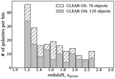
Figure 1: Redshift distribution of galaxies in the CLEAR $1.1<z<2.3$ sample in this study. This sample is selected from the 3D-HST+ parent catalog with spectroscopic redshifts from the grism data in this redshift range and by requiring that all galaxies have SNR $>$3 in [O ii], H$\beta$, or [O iii].

The selection produces a sample containing 196 galaxies. Figure 1 shows their redshift distribution. The redshifts span $1.1<z<2.3$ with a median of 1.5. The distribution is highly peaked at the first redshift bin, with $z\sim 1.25$. This is largely a result of galaxies in GOODS-N (GN), which makes up a larger number of sources (120 galaxies) in our sample compared to GOODS-S (GS, 76 galaxies). We consider two bins in redshift, each containing roughly 50% of the sample, with one bin defined with $1.1<z<1.5$ (median $z=1.3$) and the other with $1.5<z<2.3$ (median $z=1.8$). This allows us to test for redshift evolution in the properties of the sample.

Figure 2 shows the stellar-mass–SFR distribution for our CLEAR sample of $1.1<z<2.3$ galaxies using the selection criteria above, compared to the 3D–HST+ parent sample in the same redshift range. The stellar-mass distribution of the CLEAR sample is consistent with the 3D–HST+ sample when we restrict the stellar–mass range to $9.2<\log M_{\ast}/M_{\odot}<10.2$ (where both samples are reasonably complete). The SFR distributions show that the CLEAR sample here is biased toward higher SFRs, by 0.18 dex (a factor of 1.5) compared to the 3D–HST+ parent sample. The bias can be explained as a result of the emission line selection: we require galaxies to have SNR $>$3 in H$\beta$, [O ii], and/or [O iii]. The CLEAR line-flux detection limit is $2\times 10^{-17}$ erg s^-1 cm^-2 (3$\sigma$), which for H$\beta$ corresponds to SFR$\simeq$3–7 $M_{\odot}$ yr^-1 (with no dust attenuation) at $z=1.5-2.0$ (assuming the calibration of Kennicutt 1998 for a Chabrier IMF). Comparing this to Figure 2 we see that this effectively limits our study to objects with higher SFRs than the median. This bias in SFR is similar to other studies of emission-line selected studies of galaxies (cf., Shivaei et al. 2015; Sanders et al. 2018). We expect this bias to have only a minor impact on our results as previous studies have shown that a change in SFR of 1 dex corresponds to a change in metallicity of $\simeq$0.3 dex (e.g., Henry et al. 2021). Based on this argument the bias in SFR between the emission-line-selected sample and the parent sample, $\Delta(\log~{}\mathrm{SFR})\simeq 0.18$ dex (Figure 2), corresponds to $\Delta(\log Z)=0.05$ dex.

In Appendix A we also consider a subset of 87 galaxies from this sample with $1.2<z<1.5$ for which H$\alpha$+[N ii] are covered by the data. These galaxies have a median redshift $z=1.30$. We use this subsample to test how incorporating additional lines impacts the constraints on the gas-phase metallicity and ionization (cf. Henry et al. 2021).

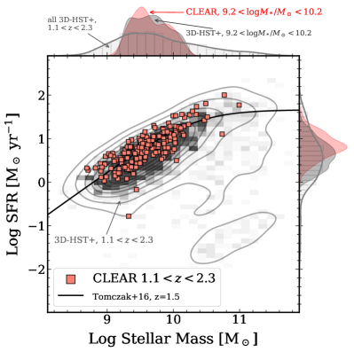
Figure 2: SFR–Stellar-Mass distributions for galaxies in our CLEAR sample. The shaded regions and contours show the distribution of sources with $1.1<z<2.3$ from the 3D–HST+ parent catalog. The red-colored squares show the CLEAR sample studied here. The plots at the top and to the right show the distributions of the samples in $\log M_{\ast}$ and $\log$ SFR using a histogram and kernel density estimator.

2.5 Estimating Galaxy Stellar Masses, Dust Attenuation, and SFRs

In what follows we compare the galaxy emission-line properties (including derived quantities such as gas-phase metallicity and ionization parameter) to galaxy stellar population parameters, including stellar masses, SFRs, and sSFRs. To derive these latter quantities we use a custom-designed method that fits stellar population synthesis models to the broad-band photometry (from our 3D-HST+ catalog, see Section 2.2) and the WFC3 G102 and G141 1D spectra (see Section 2.3). The method is discussed in detail elsewhere (Estrada-Carpenter et al. 2020, 2022), and we summarize it here.

Figure 3: Examples of model fits to the broad-band photometry and HST grism data for two example galaxies at $z~{}\sim 1.5$ in the GOODS-N CLEAR fields (GN 19659 is also shown in Figure 7). The fitting procedure uses the method of Estrada-Carpenter et al. (2020, and in prep)) The top row of each set of panels shows the broad-band photometry (green dots) from the CLEAR 3DHST+ catalog, the G102 (blue) and G141 (red) spectra along with a best-fit stellar population model (black line). The model fits currently exclude emission lines (though the emission features are prominent in the data for these galaxies). The lower set of panels for each galaxy show the posteriors for the stellar mass ($\log M/M_{\odot}$), dust attenuation ($A(V)$/mag), and specific SFR ($\log$ sSFR/yr^-1), where the vertical line shows the median and the shaded region shows the 16–84 percentile range of the HDI.

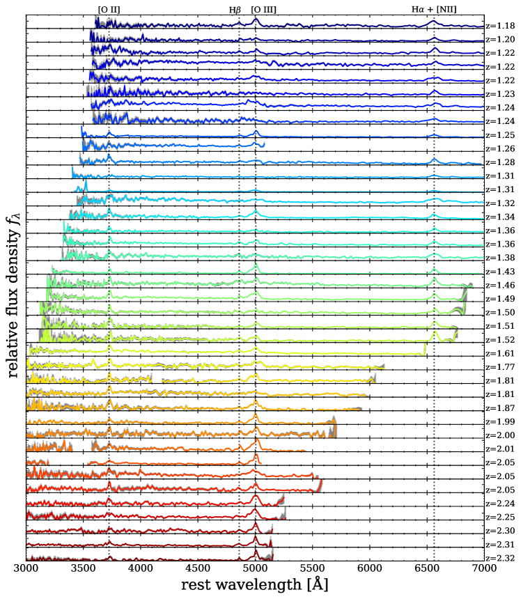
Figure 4: Gallery of individual one-dimensional G102 + G141 spectra for the sample of 40 galaxies in CLEAR with $1.1<z<2.3$ in the stellar mass range $9.6<\log M_{\ast}/M_{\odot}<9.9$ with SNR $>$3 in at least one of [O ii] $\lambda$3726,3729, [O iii] $\lambda\lambda$4959, 5008, and H$\beta$ $\lambda$4861. The spectra have been shifted to the rest-frame to illustrate common spectral features. The color scale changes with spectroscopic redshift (the gray shading of each spectrum indicates the uncertainty). For galaxies with $z\mathrel{\hbox{\hbox to0.0pt{\hbox{\lower 4.0pt\hbox{$\sim$}}\hss}\hbox{$<$}}}1.6$ the data cover H$\alpha$ $\lambda$6563 (which is blended with [N ii] $\lambda\lambda$ 6584, 6584 at the resolution of the G141 grism).

We use the FSPS models (Conroy & Gunn 2010b) with a Kroupa (2001) IMF. We fit a total of 23 parameters, including metallicity (of the stellar population, $Z_{\ast}$), age, dust attenuation ($A_{V}$, assuming the Calzetti et al. 2000 model), and a flexible star-formation history (allowing for 10 bins of SFR dynamically-spaced in time, following Leja et al. 2019). We also include 8 additional nuisance parameters to allow offsets in the normalization/calibration between the spectra and the photometry, and to allow for correlated noise between spectral data points (see Estrada-Carpenter et al. 2020, and in prep for more details). We then fit to the broad-band data and grism spectroscopy (for this modeling we currently exclude regions of strong line emission) using a Bayesian formalism with a nested sampling to predict the posteriors. We marginalize the posterior probability distribution functions to derive constrains on the stellar population parameters.

We find that excluding the emission lines from the SED fitting causes a small bias in the SFRs (and the specific SFRs) of the galaxies in our sample. We compared the SED-derived SFRs for objects in our sample to SFRs estimated from dust-corrected H$\beta$ emission measured in the grism data (assuming Case-B recombination and the calibration of Kennicutt & Evans 2012). For galaxies with SFRs $\mathrel{\hbox{\hbox to0.0pt{\hbox{\lower 4.0pt\hbox{$\sim$}}\hss}\hbox{$<$}}}$ 5 $M_{\odot}$ yr^-1 the H$\beta$-derived SFRs estimated are higher by about 0.25 dex (for galaxies with higher SFRs the bias is negligible). Because we use SED-derived specific SFRs, we ensure we are not biased toward galaxies with strong emission lines only. Furthermore, this potential bias in SFR (and specific SFR) has negligible impact on our conclusions related to the specific SFR as this bias is smaller than the trends seen in the data and remains present if we replace the specific SFR with alternative measures (such as H$\beta$ equivalent width, see Reddy et al. 2018, and Sections 5.3 and 6.4).

Using this method we fit the stellar population parameters for all the galaxies in our sample. Here we focus on the stellar population constraints for stellar mass ($M_{\ast}$), SFR, and dust attenuation ($A_{V}$) for the study here. We will present results derived from these parameters elsewhere (V. Estrada-Carpenter et al. in prep). Figure 3 shows results from the fitting for two galaxies in our sample. The figure includes the best-fit SED (with parameters that maximize the likelihood) along with the broad-band photometry and grism data. The figure also shows the marginalized posteriors for the three parameters above. We take the mode and highest density interval (HDI, Bailer-Jones et al. 2018) from the posteriors as the measurement and inter-68 percentile range (e.g., the inter–16th-to-84th percentile range) for each parameter, respectively. In what follows, we refer to these as “SED–derived” values as they were derived from fitting models to the galaxy SEDs.

3 Characteristics of Grism Spectra of Emission-Line Galaxies at ${1.1<{\mathrm{z}}<2.3}$

Figure 4 shows a gallery of the G102 + G141 1D spectra for the 40 individual galaxies in our sample in the stellar mass range $9.6<\log M/M_{\odot}<9.9$, ordered by increasing redshift. The spectra are shifted to the rest-frame to illustrate common features. The most prominent lines are [O ii] $\lambda$3726,3729, [O iii] $\lambda\lambda$4959, 5008, and H$\beta$ $\lambda$4861. For galaxies with $z\mathrel{\hbox{\hbox to0.0pt{\hbox{\lower 4.0pt\hbox{$\sim$}}\hss}\hbox{$<$}}}1.6$, H$\alpha$ $\lambda$6563 is also present. At the resolution of the G141 grism, this line is blended with the [N ii] $\lambda\lambda$ 6584, 6584 lines.

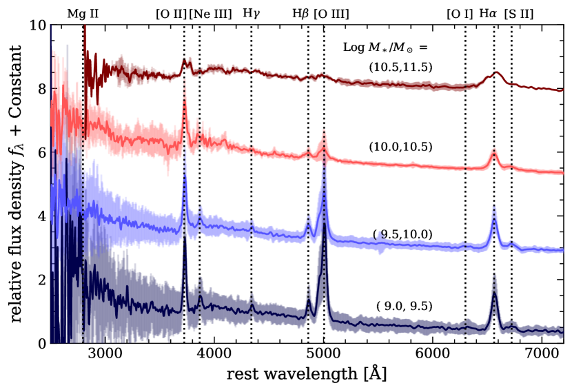
Figure 5: One-dimensional G102 + G141 spectral stacks of galaxies in the sample ($1.1<z<2.3$), divided in four bins of stellar mass. The spectra have been shifted to the rest-frame, and stacked as described in the text. The solid lines show the weighted mean of each stack and the shaded region shows standard deviation of the population (NB: this the dispersion of the objects in the stack, and not the error on the mean). The locations of prominent emission features are labeled. The stacked spectra illustrate the effects of the instrumental resolution on the emission features. The data also show that the relative strength of emission features depends on stellar mass, with galaxies with lower stellar masses having stronger emission lines, and stronger [O iii] compared to [O ii] and H$\beta$.

3.1 Stacked (Average) Spectra of CLEAR Galaxies

To facilitate with the interpretation of the HST spectra, we constructed stacked spectra for galaxies in our sample in bins of stellar mass. We first divided the galaxies into subsamples of stellar mass, $9.0<\log M_{\ast}/M_{\odot}<9.5$, $9.5<\log M_{\ast}/M_{\odot}<10$, $10<\log M_{\ast}/M_{\odot}<10.5$, and $10.5<\log M_{\ast}/\hbox{$M_{\odot}$}<11.5$. To create the stacks we corrected the spectra for dust attenuation assuming the Calzetti et al. (2000) model and the $A(V)$ values derived from the SED fits (see Section 2.5). We then shifted all 1D spectra for the galaxies to the rest-frame using the measured redshift from the grism data. We linearly interpolated the data to a wavelength grid over $2500-7500$ Å at a resolution of $\delta\lambda$=5 Å. We normalized each galaxy in the rest-wavelength range $4300-4500$ Å (a window that avoids strong emission features, following Zahid et al. 2017) and co-added the spectra, weighting by the inverse variance of the flux density. We then divided the spectra by the total weights to obtain a mean spectrum. We also created a weighted sum of the variance of the flux density in the same way to study the variation of the spectra among galaxies in the sample.

Figure 5 shows the stacked spectra of the CLEAR galaxies in the bins of stellar mass. The spectra show common features, most prominently strong emission from [O ii], [O iii], H$\beta$, and H$\alpha$. In addition, weaker lines are also evident, including [Ne III], H$\gamma$, [S II], and [O I]. The shaded region of the stacked spectra in the figure shows the scatter of the population in each stack (i.e., this is not the uncertainty on the mean). The shading indicates the scatter is generally larger at shorter wavelengths, which we attribute to variations in star-formation histories (although some of this may be caused by the lower sensitivity of the G102 grism at bluer wavelengths).

In general, the strength of the spectral features increases with decreasing stellar mass. In particular, it is in the lowest mass galaxies ($9.0<\log M_{\ast}/M_{\odot}<9.5$) where the strongest emission is seen, and where weaker lines such as [Ne III] and H$\gamma$ become prominent. The relative strength of [O iii]/[O ii] also increases with decreasing stellar mass. This is an indication of increasing gas ionization and/or decreasing gas-phase oxygen abundance. We will explore this quantitatively below.

Table 1: Relative Emission Line Flux Ratios and Line Equivalent Widths from Stacked Spectra of CLEAR Galaxies at $1.1<z<2.3$

. Number EW H$\beta$ EW H$\gamma$ EW H$\epsilon$ sample of galaxies $\langle\hbox{$12+\log(\mathrm{O/H})$}\rangle$ log R₂₃ log O₃₂ log [Ne iii]/[O ii] [Å] [Å] [Å] Stacked Spectra of Galaxies in bins of Stellar Mass $\log M_{\ast}/M_{\odot}>10.5$ 9 8.83 $\pm$ 0.05 0.55 $\pm$ 0.06 $-$0.40 $\pm$ 0.12 $<-1.33$ 21.9 $\pm$ 1.0 04.3 $\pm$ 1.1 2.5 $\pm$ 1.1 $\log M_{\ast}/M_{\odot}=[10,10.5)$ 36 8.65 $\pm$ 0.03 0.70 $\pm$ 0.06 $-$0.15 $\pm$ 0.11 $-$1.18 $\pm$ 0.12 23.6 $\pm$ 1.2 09.7 $\pm$ 1.0 4.7 $\pm$ 1.1 $\log M_{\ast}/M_{\odot}=[9.5,10)$ 84 8.55 $\pm$ 0.02 0.80 $\pm$ 0.03 +0.07 $\pm$ 0.11 $-$1.03 $\pm$ 0.17 44.2 $\pm$ 1.9+ 16.3 $\pm$ 2.0+ 4.7 $\pm$ 1.7+ $\log M_{\ast}/M_{\odot}=[9.0,9.5)$ 66 8.42 $\pm$ 0.03 0.92 $\pm$ 0.03 +0.27 $\pm$ 0.11 $-$0.87 $\pm$ 0.19 49.6 $\pm$ 3.8+ 18.5 $\pm$ 3.2+ 8.0 $\pm$ 3.5+ Stacked Spectra of Galaxies with High- and Low-Ionization Parameters, all with $\log M_{\ast}/M_{\odot}=[9.3,9.7]$ and $\hbox{$12+\log(\mathrm{O/H})$}>8.3$ High-ionization, 31 8.49 $\pm$ 0.04 0.89 $\pm$ 0.01 +0.35 $\pm$ 0.11 $-0.96$ $\pm$ 0.11 61.3 $\pm$ 0.6 23.7 $\pm$ 0.5 8.2 $\pm$ 0.5 $\log q>7.8$ Low-ionization, 32 8.52 $\pm$ 0.04 0.86 $\pm$ 0.03 $-$0.03 $\pm$ 0.11 $-1.12$ $\pm$ 0.11 35.4 $\pm$ 0.5 13.0 $\pm$ 0.4 4.4 $\pm$ 0.5 $\log q<7.8$

Note. — All line ratios and emission line equivalent widths are measured from the stacked spectra using pPXF  as described in the text (Sections 3.2 and 6.4). Equivalent widths are in measured in the rest-frame.

3.2 Measuring Emission Line Ratios from Stacked Spectra

Because of this sizable variation in the spectral properties of the galaxies even at fixed stellar mass, we opt to study the individual spectra in most of the analysis that follows. However, we also use emission line ratios and equivalent width measurements from the stacks to interpret the average evolution of galaxies as a function of stellar mass and gas-phase metallicity. This complements work that analyzes the average properties of galaxies from stacked HST WFC3 grism spectra (including, e.g., Henry et al. 2021, which in part uses stacks that include the same data used here).

To measure the emission line fluxes from stacked spectra in Figure 5 we adapted the Penalized Pixel-Fitting method (pPXF, Cappellari 2017) for the CLEAR data. The primary difference between our use of pPXF and other datasets is that the CLEAR WFC3 grism data are lower resolution ($R\sim 100-200$) than other spectroscopic studies (see, Cappellari 2017). Nevertheless, pPXF fits simultaneously the stellar components and nebular emission (i.e., correcting the nebular emission for stellar absorption), fitting for the line width (which is important here as our stacks include individual spectra with different spectral resolution owing to the morphological broadening). And, pPXF can separate the Balmer emission from the metal emission features. For our purposes, we added to pPXF the [Ne iii] $\lambda$3868 emission line as this is prominent in our data (Figure 5). We then ran pPXF  on the stacked data in Figure 5 (using stacks where the input spectra have been corrected for dust attenuation). We ran pPXF  in two modes: one where each Balmer emission line is fit separately and one where we tie the Balmer emission lines to their theoretical Case-B values (e.g., Osterbrock 1989), and we use the latter for cases where H$\gamma$ is too weak to be visible in the spectra. We report the results in Table 1. Because the flux density in the stacked spectra have been normalized we report emission line flux ratios and equivalent widths (EWs) of prominent features. We use these results in the Section 6.4 to interpret the bulk trends between emission-line ratios and galaxy properties.

4 Gas-Phase Metallicity and Ionization from Nebular Emission Lines

The WFC3 grism data cover emission lines in the rest-frame optical (for galaxies at $1.1<z<2.3$) that are sensitive to nebular ionization and gas-phase metallicity. The lower spectral resolution of the HST/WFC3 G102 and G141 data ($R\sim 100-200$) cause the O II $\lambda\lambda 3726,~{}3729$ and O III $\lambda\lambda 4959,~{}5008$ lines to be blended (see Figure 5). Rather than attempting to de-confuse these lines, we adopt line ratios that make use of the sums of these lines. Specifically we define ratios of these lines as:

$$\mathrm{O}_{32} \equiv \frac{\hbox{[O\,{\sc iii}]}~{}\lambda\lambda 4959,~{}5008}{\hbox{[O\,{\sc ii}]}~{}\lambda\lambda 3726,~{}3729}$$ (1)

$$\mathrm{R}_{23} \equiv \frac{\hbox{[O\,{\sc iii}]}~{}\lambda\lambda 4959,~{}5008+\hbox{[O\,{\sc ii}]}~{}\lambda\lambda 3726,~{}3729}{\hbox{H$\beta$}\lambda 4861},$$ (2)

where $\hbox{[O\,{\sc iii}]}~{}\lambda\lambda 4959,~{}5008$ and $\hbox{[O\,{\sc ii}]}~{}\lambda\lambda 3726,~{}3729$ are the sum of the emission from both lines in the doublet, where we have corrected the line fluxes for dust attenuation using the $A(V)$ values from the SED fits with the Calzetti et al. (2000) model. The line ratio $\mathrm{O}_{32}$ is sensitive to the ionization of the gas (as it measures the relative amount of emission from double-ionized oxygen to singly ionized oxygen, see Strom et al. 2018; Kewley et al. 2019b). The line ratio $\mathrm{R}_{23}$ is sensitive to the gas-phase metallicity (specifically the oxygen abundance, $12+\log(\mathrm{O/H})$) as for the typical conditions in H II regions the majority of the gas-phase oxygen is in the singly or doubly ionized states (e.g., Delgado-Inglada et al. 2014; Kewley et al. 2019b). In Appendix A, we test how including measurements of $\hbox{H$\alpha$}+\hbox{[N\,{\sc ii}]}$ (which is the sum of $\hbox{H$\alpha$}~{}\lambda 6564+\hbox{[N\,{\sc ii}]}~{}\lambda\lambda 6548,~{}6583$) and [S ii] (which is unresolved in the grism data, therefore we use the sum of the lines in the [S ii]$\lambda\lambda 6716,~{}6731$ doublet) impact our results, and we find there is no substantive change to our conclusions.

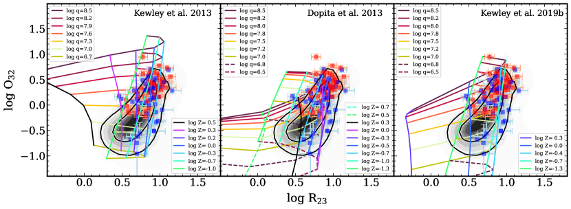
Figure 6: Top panel: Distribution of O₃₂ as a function of $R_{23}$ for galaxies in the CLEAR sample (colored squares) compared to that from SDSS (using a kernel density estimator [KDE], gray shaded region; the contours contain 50% and 80% of the SDSS sample). For clarity, the plot only shows CLEAR galaxies with SNR $>$3 in [O ii], [O iii], and H$\beta$, color-coded by redshift. The data have been corrected for dust attenuation (see Section 4). The CLEAR galaxies reside in the upper end of the SDSS distribution. The panels to the top and right show the one-dimensional distributions from a KDE. Bottom panels: the distribution of the CLEAR and SDSS R₂₃ versus O₃₂ distributions compared to predictions from photoionization models considered here. In this work we adopt the MAPPINGS V models (Kewley et al. 2019b) as these are the most current at the time of this writing, and they best cover the line ratios spanned by the observed galaxies.

4.1 Comparison to Photoionization Models

Figure 6 compares the distribution of R₂₃ and O₃₂ for galaxies in the CLEAR sample to those from SDSS DR14 (Thomas et al. 2013). For both SDSS and CLEAR galaxies, the emission lines have been corrected for dust extinction. For SDSS, we used the values provided by Thomas et al.. For our CLEAR galaxies, we corrected the line ratios using dust attenuation estimates from our SED fitting to the grism spectra and photometry (see Section 2.5) as most galaxies in our sample do not have measurements of multiple Balmer emission lines. We also assume the Calzetti et al. (2000) attenuation law and that the attenuation in the nebular gas is the same as for the stellar continuum (c.f. Reddy et al. 2015).

The CLEAR galaxies at $1.1<z<2.3$ lie at the upper end of the R₂₃–O₃₂ distribution defined by SDSS (the latter is shown using a kernel density estimator [KDE]). This is similar to the findings of other studies of high redshift galaxies (e.g., Sanders et al. 2016; Strom et al. 2018; Runco et al. 2021), which interpret the data as an increase in ionization parameter, harder ionizing spectrum, decrease in metallicity, and possibly elevated nitrogen abundances and higher $\alpha$/Fe abundance ratios. The CLEAR galaxies support many of these assertions and we discuss these further below (see, Section 6.4).

Figure 6 also compares the line ratios to photoionization models. The models include the Dopita et al. (2013) models, which used the MAPPINGS IV code (bottom row, middle panel of the Figure). The Dopita et al. model includes updated atomic data, elemental abundance measurements, and modeling prescriptions. The input ionizing spectrum uses the STARBURST99 population synthesis model (Leitherer et al. 2014) for a stellar population with a constant SFR, observed at an age of 4 Myr, with a Salpeter IMF with an upper-mass cutoff of 120 $M_{\odot}$. The nebular region also assumes spherical geometry, isobaric photoionization, and that the distribution of electron velocities allows for an extended tail to higher energies (a so-called “$\kappa$” distribution). These models span the range of R₂₃–O₃₂ observed in the SDSS and CLEAR data, although the models are unable to produce the highest ratios (e.g., the models are limited to R${}_{23}\mathrel{\hbox{\hbox to0.0pt{\hbox{\lower 4.0pt\hbox{$\sim$}}\hss}\hbox{$<$}}}1$ while galaxies with R${}_{23}>1$ are evident in the SDSS and CLEAR data).

The Kewley et al. (2013) models in Figure 6 (bottom row, left panel) show the effects of using the PEGASE 2 (Fioc & Rocca-Volmerange 1999) population synthetic models that include harder ionizing spectra (e.g., Kewley et al. add the spectra of planetary nebular nuclei for stars with high effective temperatures, $T_{e}>50,000$ K to estimate for the effects of the stellar photospheres of massive stars). These models increase the ratios of O₃₂ in response to the increased ionization parameter. Nevertheless, these models also have difficulty achieving the highest R₂₃ values seen in the data.

Figure 6 also shows line ratios for the MAPPINGS V models (Kewley et al. 2019b, a) (bottom row, right panel). The MAPPINGS V models include updates with the latest atomic data and relative abundances (see, Nicholls et al. 2017). The input spectrum is based on the STARBURST99 stellar population synthesis models (as above) using models for massive stars (Hillier & Miller 1998; Pauldrach et al. 2001) that are able to produce better the ratios of blue/red supergiants in low-metallicity regions, such as the Magellanic Clouds.

Importantly, the MAPPINGS V models are isobaric, and consider the effects of different values for the ISM pressure, here defined as $P/k=n_{e}T$ (in units of K cm^-3, where $n_{e}$ and $T$ are the nebular electron density and temperature). In the present work, we adopt $\log P/k=6.5$ as this represents well the expected conditions in high-redshift galaxies (see, e.g., Acharyya et al. 2019). For example, Sanders et al. (2016) and Kaasinen et al. (2017) find evidence for higher median electron density, $n_{e}\simeq 250-300$ cm^-3 (where $n_{e}\approx n_{\mathrm{H}}$ for ionized gas) for $\sim 1-3$ galaxies (see also, Runco et al. 2021). Combined with the expected nebular temperature of $\sim$10,000–20,000 K (see, Andrews & Martini 2013; Sanders et al. 2020, and references therein), this implies a gas pressure of $\log P/k\sim 6.5-7.0$. Figure 6 shows the MAPPINGS V models assuming $\log P/k=6.5$, but we observe similar results for $6<\log P/k<7.5$. Models with $\log P/k$=6.5 and 7.0 reproduce the span of the data as illustrated in the Figure. Models with $\log P/k=6.0$ do not reproduce the data with the highest O₃₂ ratios, while models with higher pressure ($\log P/k$=7.5) produce lower R₂₃. We therefore adopt $\log P/k=6.5$ for our analysis while noting that changing this from 6.0–7.5 does not alter our conclusions.

The MAPPINGS V models still have difficulty producing the highest R₂₃ values seen in the data (i.e., those with $\log R_{23}\mathrel{\hbox{\hbox to0.0pt{\hbox{\lower 4.0pt\hbox{$\sim$}}\hss}\hbox{$>$}}}1$ in both SDSS and CLEAR, see Fig. 6). This effect has been seen in other studies. To explain this offset could require stellar populations with enhanced $\alpha$/Fe ratios (e.g., Sanders et al. 2016; Steidel et al. 2016; Strom et al. 2022), or a change in nebular geometry (e.g., “density” bounded nebula [Brinchmann et al. 2008; Nakajima & Ouchi 2014; Kashino & Inoue 2019], or clumpy geometries [Jin et al. 2022]). This highlights the need for improvements in photoionization models to fully account the range of line emission observed in high redshift galaxies. We plan to investigate this in a future study.

Figure 7: Gallery of HST RGB images (using ACS F775W, WFC3 F105W and F160W imaging), grism spectra, and derived constraints on the gas-phase metallicity ($12+\log$ O/H) and ionization ($\log q$). The figure includes galaxies in the CLEAR GOODS-N pointings with redshift $1.2<z<1.5$ such that the spectra contain [O ii], H$\beta$, [O iii], and H$\alpha$+[N ii]. Each row shows one galaxy. The left-most panel shows the RGB image. The scale bar corresponds to one arcsecond. The middle panel shows the 1D, G102 (blue) and G141 (red), extracted spectra, prominent emission features are indicated. The right-most two panels adjacent to each spectrum show the posterior on the gas-phase metallicity ($12+\log(\mathrm{O/H})$) and ionization parameter ($\log q$) derived by comparing the [O ii], H$\beta$, and [O iii] line fluxes against the MAPPINGS V photoionization models. The solid and dashed vertical lines show the mode and 68% range derived for the highest density interval (HDI Bailer-Jones et al. 2018). The galaxies are sorted as a function of decreasing stellar mass (top to bottom).

Figure 8: Same as Figure 7, but showing example galaxies with spectroscopic redshifts $1.3<z<1.9$ in the CLEAR GOODS-S pointings. The galaxies are sorted as a function of decreasing stellar mass (top to bottom).

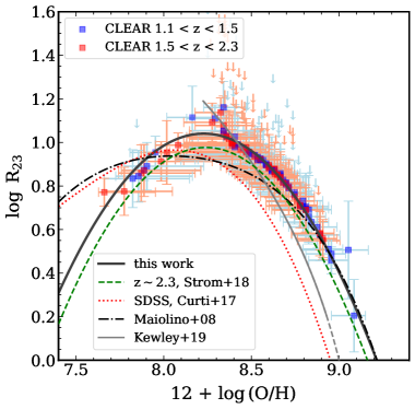
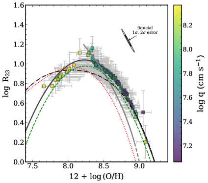
Figure 9: Metallicity versus $R_{23}$ for the CLEAR sample derived by comparing the observed [O ii], H$\beta$, and [O iii] line fluxes to MAPPINGS V photoionization models. The data points show the mode of the posterior likelihoods on metallicity. The error bars denote the inner-68 percentiles derived from the highest density intervals; arrows show $1\sigma$ limits. The curves denote various calibrations in the literature (Maiolino et al. 2008; Curti et al. 2017; Strom et al. 2018; Kewley et al. 2019b); the solid-thick line is our fit to the CLEAR results (see Eq. 3). The left panel shows the CLEAR galaxies colored by redshift. The right panel shows the CLEAR galaxies colored by ionization, $\log q$. While there is a trend between $R_{23}$ and metallicity, there is an additional dependence on ionization $q$. The $12+\log(\mathrm{O/H})$ values are derived using the line fluxes in R₂₃, which causes the apparently “tight” scatter data points relative to their error bars. To illustrate this, we show example error ellipses for a fiducial galaxy with 12 + log(O/H) = 8.8. These illustrate the covariance between R₂₃ and $12+\log(\mathrm{O/H})$ lies in the direction of the relation.

4.2 Estimating the Gas-Phase Metallicity and Ionization Parameter

We use the code, “Inferring the gas phase metallicity ($Z$) and Ionization parameter” (IZI) developed by Blanc et al. (2015) to estimate the metallicity ($Z$, which we take to be the nebular oxygen abundance, 12 + $\log$(O/H)) and ionization parameter ($q$). IZI is a Bayesian code which computes posterior likelihoods for $Z$ and $q$ by comparing the measured emission line fluxes for our galaxies to predictions from the photoionization models. IZI is flexible in the sense that it can use any combinations of lines, including the summed fluxes of multiple lines (which is useful in our case where emission lines are blended at the resolution of the WFC3 grisms).

We use MAPPINGS V models (Kewley et al. 2019b) assuming a isobaric pressure in the nebula of $\log P/k=6.5$ (K cm^-3 for the reasons in Section 4.1. We adapted the output of the MAPPINGS V models into the format required for IZI. We assume a “flat” prior for both $\log Z$ and $\log q$, spanning the ranges $-1.3\leq\log Z/Z_{\odot}\leq 0.3$ and $6.5<\log q/(\mathrm{cm~{}s^{-1}})<8.5$. We tested alternative pressure values from $\log P/k=6-7.5$ and find no substantial differences in our conclusions. We also tested the use of different priors (including a prior with the shape of the local- and high-redshift mass–metallicity relation [Maiolino et al. 2008; Andrews & Martini 2013; Henry et al. 2021; Sanders et al. 2021]). These priors only change slightly the shape of the posteriors of lower-mass galaxies (shifting the inter-68 percentile range to higher values of metallicity by $<$0.1 dex) while leaving the median values nearly unchanged (at fixed stellar mass). Moreover, adopting a prior affects the MZR, changing the average metallicity of galaxies at $\log M_{\ast}/M_{\odot}$=9.5 by $<$0.01 dex (Section 5.1). We therefore adopt the results from the “flat” prior to avoid any bias inflicted by the prior information, but this has a minimal impact on our conclusions.

We focus on results that use the sum of the emission from [O ii]$\lambda\lambda 3726$, 3729 doublet, the sum of the emission from [O iii]$\lambda\lambda 4959$, 5008, and the emission from H$\beta$ as these lines are available over our full redshift range of our sample, and they constrain both the ionization state of the gas and trace the majority of nebular oxygen. In all cases we correct the line emission for dust attenuation as in Section 4.1. In Appendix A, we compare these results to the case where we also include the emission from H$\alpha$+[N ii]$\lambda\lambda$6548, 6583 and [S ii]$\lambda\lambda$6716, 6731 with the emission from [O ii], [O iii], and H$\beta$ for galaxies at $1.1<z\mathrel{\hbox{\hbox to0.0pt{\hbox{\lower 4.0pt\hbox{$\sim$}}\hss}\hbox{$<$}}}1.6$ where all these lines are also covered by the WFC3 grisms. Adding these lines does not change our interpretation, though it does provide additional confidence in the results derived from only the [O ii], [O iii], and H$\beta$ lines.

We show examples of the results in Figures 7 and 8 for galaxies in GOODS-N and GOODS-S, respectively. For each galaxy in the figure we show the image (ACS F775W, WFC3 F105W and F160W) along with the 1D spectrum from the G102 + G141 grisms. The right-most panels show the posteriors on gas-phase metallicity (12 + log O/H) and ionization $\log q$ (in units of cm s^-1) derived from IZI for each galaxy. Because the images show the same observed bands, color differences indicate the presence of the strong emission lines, spectral breaks, or spatially variant dust effects as they redshift through the filters. For example, for $z\mathrel{\hbox{\hbox to0.0pt{\hbox{\lower 4.0pt\hbox{$\sim$}}\hss}\hbox{$>$}}}1.6$ the 4000 Å/Balmer break shifts redward of the F105W band. This accounts for the redder appearance of some galaxies (such as GS 28878). In other cases, the [O iii] emission line shifts into the F160W filter for $z\mathrel{\hbox{\hbox to0.0pt{\hbox{\lower 4.0pt\hbox{$\sim$}}\hss}\hbox{$>$}}}1.8$, which accounts for the redder appearance of other galaxies (such as GN 32485).

In what follows we report the mode for the metallicity and ionization using the $P(\log Z)$ (where we use $\log Z=12+\log\mathrm{O/H}$ here) and $P(\log q)$ distributions, along with the 16th percentile and 84th percentile to indicate the uncertainties. We derive the latter using the HDI, which is the smallest region that contains 68% of the probability density (see Bailer-Jones et al. 2018; Estrada-Carpenter et al. 2020). These are indicated by the vertical lines in the $P(\log Z)$ and $P(\log q)$ panels for each galaxy in Figures 7 and 8.

4.3 The relation between strong-line ratios and metallicity

Figure 9 shows our results for the metallicity ($12+\log\mathrm{O/H}$) derived from the R₂₃ line ratio. The data points show the results for individual CLEAR galaxies with metallicities and ionization derived using IZI from the strong emission lines. The curves in the Figure show calibrations from the literature, derived using different methods and galaxy samples. It should be noted that the errors on the data points in the Figure are highly covariant (as the metallicity values are derived from the $R_{23}$ ratios). To illustrate this, the right panel of Figure 9 shows the equivalent $1\sigma$ and $2\sigma$ error ellipses derived from the covariance between these parameters for a fiducial galaxy in the sample with $\hbox{$12+\log(\mathrm{O/H})$}=8.8$. This accounts for the lack of perceived scatter in the results (the scatter is covariant as indicated by the error ellipse, and is directed along the observed sequence between R₂₃ and metallicity).

The R₂₃–metallicity calibrations include those based on nearby star-forming galaxies (e.g., SDSS galaxies at $z\sim 0.1$, Maiolino et al. 2008; Curti et al. 2017). Maiolino et al. used a combination of direct measurements (for low-metallicity galaxies) with metallicities inferred from photoionization models for higher metallicity galaxies in SDSS. These results show that R₂₃ is famously “double-valued” with a maximum and inflection point around $\log$ R${}_{23}\simeq 1$ at $12+\log\mathrm{O/H}\simeq 8.2$. On the high-metallicity branch of R₂₃, other calibrations find lower metallicity at fixed R₂₃ using direct $T_{e}$ metallicity methods (Curti et al. 2017), but those authors caution that the [O iii] $\lambda 4363$ emission exhibits contamination from [Fe II] emission in higher metallicity regions. In addition, other studies have argued that some of the offset may result from a contribution to the emission from diffuse interstellar gas (DIG, Sanders et al. 2017), but at these redshifts this effect is expected to be small (Sanders et al. 2021)). Yet other studies find that the assumption about the ionization of the gas leads to biases that cause the metallicity derived from R₂₃ to be undervalued (Berg et al. 2021).

The effect of the (isobaric) pressure of the nebular gas is also important. Kewley et al. (2019b) use the suite of predictions from MAPPINGS V with a gas pressure of $\log P/k=5$, valid for $8.53<\hbox{$12+\log(\mathrm{O/H})$}<9.23$. These calibrations have a dependence on ionization parameter. These models produce the calibration illustrated in Figure 9 (thick gray line). These are consistent with the Curti et al. (2017) calibration. Increasing the pressure to $\log P/k=7$ has a strong impact on $\log R_{23}$ for metallicities $\hbox{$12+\log(\mathrm{O/H})$}\mathrel{\hbox{\hbox to0.0pt{\hbox{\lower 4.0pt\hbox{$\sim$}}\hss}\hbox{$>$}}}8.5$ (see Kewley et al. 2019b, their Figure 9), increasing $\log R_{23}$ by nearly $\sim$1 dex at $\hbox{$12+\log(\mathrm{O/H})$}\sim 9$. Because we use an isobaric pressure of $\log P/k=6.5$, this explains the offset in our calibration and that of Kewley et al. and Curti et al., illustrated in the figure. Our calibration is more consistent with that derived independently by Strom et al. (2018).

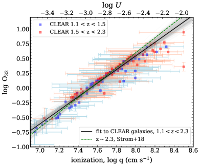
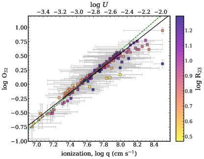
Figure 10: O₃₂ versus ionization for the CLEAR sample, derived by comparing the observed [O ii], H$\beta$, and [O iii] line fluxes to the MAPPINGS V photoionization models. The left panel shows CLEAR galaxies color coded by redshift. The right panel shows the CLEAR galaxies color coded by R₂₃ value. In each panel, the top axis shows the corresponding dimensionless ionization parameter ($U=q/c$). The dashed line shows the linear relation calibrated by Strom et al. (2018) using independent photoionization modeling for $z\sim 2.3$ galaxies. The solid line shows a linear fit to the CLEAR galaxies derived from a Bayesian method. The shaded gray region shows 400 random draws from the posterior of the linear fit. The O₃₂ ratio correlates with ionization parameter. There is a secondary dependence on R₂₃ (which translates to a dependence on gas-phase metallicity).

We fit a quadratic function to the R₂₃–$Z$ relation derived for the CLEAR galaxies of the form,

$$\log\mathrm{R}_{23}=A\times(\log Z-\log Z_{0})^{2}+\log\mathrm{R}_{0},$$ (3)

where $\log Z\equiv 12+\log(\mathrm{O/H})$ and $A=-1.07\pm 0.03$, $\log\mathrm{R}_{0}=1.041\pm 0.004$, and $\log Z_{0}=8.228\pm 0.006$. We include the statistical uncertainties when performing the fit. However, we have not included the effects of the covariance between R₂₃ and $Z$ (as discussed above), and therefore the uncertainties on these parameters are overestimated.

This relation we observe for CLEAR is consistent with other studies of high-redshift galaxies, that also show larger R₂₃ at fixed metallicity compared to calibrations derived for nearby galaxies. For example, Strom et al. (2018) fit strong emission lines measured in $z\sim 2.3$ galaxies using predictions from photoionization models that allow for a range of stellar and nebular metallicity, ionization parameter and N/O abundance. They then parameterize R₂₃–$Z$ as a quadratic expression, which is also shown in Figure 9. The Strom et al. relation is similar to the one for CLEAR, with an offset of 0.05–0.1 dex. The results from Strom et al. are similar to those from Maiolino et al. (although Strom et al. argue that the Maiolino et al. and other calibrations based on direct $T_{e}$ measurements need to be revised upwards by 0.24 dex).

Figure 9 also shows that for the CLEAR sample the ionization of the gas increases as the metallicity decreases. The ionization constraints (primarily from $\hbox{[O\,{\sc iii}]}/\hbox{[O\,{\sc ii}]}$) within the IZI fitting allow us to determine a likelihood that galaxies fall on the upper or lower branch of the R₂₃–$Z$ relation. Galaxies on the lower-metallicity branch of R₂₃ have significantly higher ionization than galaxies on the upper-metallicity branch of R₂₃. Physically, the change in ionization causes an increase in the fraction of doubly ionized oxygen (O⁺⁺ ) at the expense of singly ionized oxygen (O⁺), which therefore leaves the numerator in the definition of R₂₃ mostly unchanged. However, the change in ionization should then be apparent in the ratio of O₃₂, which we discuss in the next subsection.

4.4 The relation between strong-line ratios and ionization

Figure 10 shows there is a tight correlation between the O₃₂ ratio and the ionization parameter, $q$, derived by modeling the emission lines of the CLEAR galaxies with the MAPPINGS V photoionization models (Section 4.2). The correlation is expected as an increase in ionization parameter corresponds to an increase in the ratio of O⁺⁺ to O⁺. Low-redshift star-forming galaxies typically have ionization parameters in the range, $7.3<\log q/(\mathrm{cm~{}s^{-1}})<7.6$ (Moustakas et al. 2010; Poetrodjojo et al. 2018), while H II regions and super-star clusters in starburst galaxies (e.g., M82) have ionization parameters as high as $\log q/(\mathrm{cm~{}s^{-1}})\sim 8.2-8.7$ (Smith et al. 2006; Pérez-Montero 2014), which is observed in other low redshift, extreme star-forming galaxies (e.g., Berg et al. 2021; Olivier et al. 2021). For the CLEAR galaxies at $1.1<z<2.3$, the range of ionization parameter extends over $7.3\mathrel{\hbox{\hbox to0.0pt{\hbox{\lower 4.0pt\hbox{$\sim$}}\hss}\hbox{$<$}}}\log q/(\mathrm{cm~{}s^{-1}})\mathrel{\hbox{\hbox to0.0pt{\hbox{\lower 4.0pt\hbox{$\sim$}}\hss}\hbox{$<$}}}8.5$, spanning the full range seen in star-forming galaxies in the local universe. This is consistent with other studies of high redshift galaxies that show evidence for increased ionization (e.g., Sanders et al. 2016; Strom et al. 2018).

We fit a linear relation between $\log$ O₃₂ and $\log q$ using

$$\log q=A\times\log\mathrm{O}_{32}+\log q_{0}.$$ (4)

We fit the relation using a Gaussian Mixture Model (linmix, Kelly 2007), which yields $A=0.86\pm 0.07$ and $\log q_{0}=7.53\pm 0.02$. This line is shown in Figure 10 (along with 400 random draws from the posterior). This linear fit is very similar to that from Strom et al. (2018), who derived their relation from a sample of $z\sim 2.3$ star-forming galaxies with independent photoionization modeling (see also Footnote 4).

Closer inspection of the CLEAR galaxies in Figure 10 shows that while [O iii]/[O ii] correlates with ionization parameter, there is a secondary effect. The effect is subtle (with galaxies with lower R₂₃ shifting above the relation at lower ionization and below the relation at higher ionization). This effect is likely a result of the fact that many of the galaxies in our sample lie at the peak of the R₂₃–$Z$ relation ( near R${}_{23}\sim 1$ in Figure 9). R₂₃ correlates with gas-phase metallicity, this translates to a secondary effect in $12+\log(\mathrm{O/H})$. Empirically, this secondary dependence on R₂₃ comes from the relative strength of H$\beta$ compared to [O ii] + [O iii]. Galaxies with stronger H$\beta$ push toward lower R₂₃. This is predicted by the photoionization modeling (see Figure 7 of Kewley et al. 2019b), and physically is a result of the fact that gas cooling is more efficient in higher metallicity environments. While the CLEAR galaxies in Figure 10 show an apparent ceiling, with $\log\mathrm{O}_{32}\mathrel{\hbox{\hbox to0.0pt{\hbox{\lower 4.0pt\hbox{$\sim$}}\hss}\hbox{$<$}}}0.75$, this seems only a property of our sample. For example, some extreme galaxies at $z\sim 0.01$ with low metallicity ($\hbox{$12+\log(\mathrm{O/H})$}\simeq 7.4-7.6$) have even higher line ratios ($\log\mathrm{O}_{32}\simeq 1.1-1.3$) with high ionization parameters ($\log U\simeq-2.4$ to $-1.8$, Berg et al. 2021). This is consistent with our relation (Equation 4), which would predict $\log U\simeq-2.0$ to $-1.8$ for these galaxies. Taken together, this is evidence that while to first order the $\log$ O₃₂ ratio traces gas ionization strongly there is a secondary dependence on metallicity that contributes to the scatter in this relation, and this persists at high redshift ($1\mathrel{\hbox{\hbox to0.0pt{\hbox{\lower 4.0pt\hbox{$\sim$}}\hss}\hbox{$<$}}}z\mathrel{\hbox{\hbox to0.0pt{\hbox{\lower 4.0pt\hbox{$\sim$}}\hss}\hbox{$<$}}}2$).

5 Results

5.1 On the Mass-Metallicity Relation

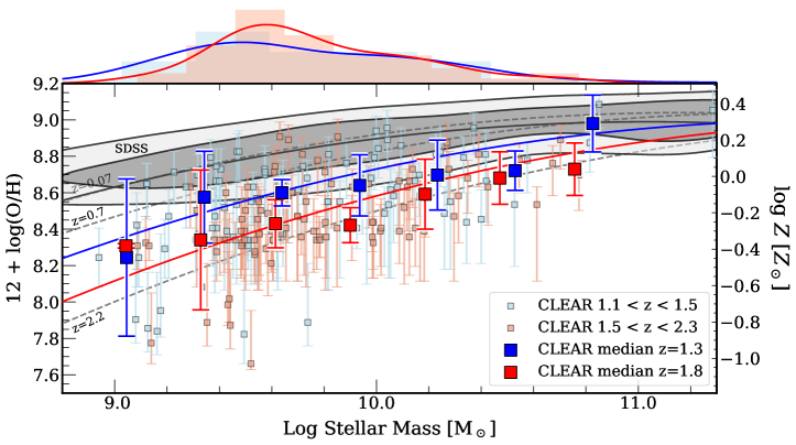
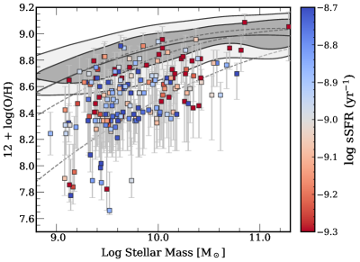
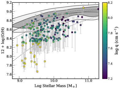
Figure 11: The stellar-mass, gas-phase-metallicity relation (MZR) for CLEAR galaxies at $1.1<z<2.3$. The top plot shows the MZR with the CLEAR galaxies color coded by redshift. Large squares show medians in bins of stellar mass. Error bars show the scatter in each bin. The red and blue solid lines show fits to the CLEAR galaxies. The gray-shaded region shows the distribution for SDSS galaxies derived using our analysis (identical to that applied to CLEAR). The black solid curve shows our quadratic fit to the SDSS galaxies (Equation 5 and Table 2). The dotted lines show the MZR relation at $z=0.07$, 0.7, and 2.2 derived by Maiolino et al. (2008). The histogram and curve along the top of the panel shows the distribution of stellar mass in the $z\sim 1.3$ (blue) and $z\sim 1.8$ CLEAR samples. The bottom panels show the MZR with galaxies color-coded by specific SFR (bottom left; $\log$ sSFR ) and nebular ionization (bottom right; $\log q$).

Figure 11 shows the relation between stellar–mass, and gas-phase metallicity (the “MZR”) derived for the galaxies in CLEAR at $1.1<z<2.3$ compared to some relations in the literature at low and high redshift. We also show results for SDSS DR14 using results derived from the same set of photoionization models and emission line fluxes as for CLEAR (see Section 4.2). Figure 11 shows that the gas-phase metallicities for the SDSS galaxies derived for these models mostly follows those derived by other methods (notably, Tremonti et al. 2004 and Maiolino et al. 2008, the latter is illustrated in the figure). Comparing these results, there is evolution from the relation from SDSS ($z\sim 0.2$) compared to CLEAR. Galaxies at higher redshift have lower metallicities, and this has been observed by multiple studies (using a myriad of methods to derive gas-phase abundances, e.g., Maiolino et al. 2008; Maiolino & Mannucci 2019; Henry et al. 2021; Sanders et al. 2021, and references therein).

To measure the evolution in the MZR, we parameterize the relation using the prescription of Maiolino et al. (2008),

$$12+\log\mathrm{O/H}=-0.0864(\log M_{\ast}-\log M_{0})^{2}+K_{0}.$$ (5)

Here, $\log M_{0}$ is a scale stellar mass (in units of Solar masses) when the relation achieves metallicity $K_{0}$. Figure 11 shows the relations derived by Maiolino et al. for SDSS and the AMAZE samples at $z=0.07$, 0.7, and 2.2 (as labeled), using an independent strong-line calibration (Kewley & Dopita 2002) calibrated against SDSS DR4 observations.

We fit Equation 5 to the results for our SDSS and CLEAR samples. For both SDSS and CLEAR we have modeled the same set of emission lines ([O iii]$\lambda\lambda$4959+5007, [O ii] $\lambda\lambda 3726$+3728, H$\beta$) with the same photoionization models (see Section 4.2). These are independent from the calibration used by others (e.g., Maiolino et al. 2008). For SDSS, because we have sufficient dynamical range in stellar mass we fit for both $M_{0}$ and $K_{0}$. However, because the stellar-mass distribution of CLEAR is strongly focused on $\log M_{\ast}/M_{\odot}\sim 9.3-9.9$ we fix $K_{0}=9.00$ at the value derived we derive from SDSS and equal to that obtained by Maiolino et al. (2008) at $z=2.2$. For CLEAR, we also fit for $M_{0}$ for subsamples of galaxies split in redshift for $1.1<z<1.5$ and $1.5<z<2.3$.

It is worth noting that the MZR relation we derive for SDSS (Figure 11, solid gray line) agrees well with the relation derived by Maiolino et al. (2008) (dashed gray line). This comparison is important because we have used a different photoionization model, and different choices of strong emission lines. Maiolino et al. (2008) calibrate their metallicities using photoionization models that assume lower $n_{e}$, which result in lower pressure. Nevertheless, the calibrations agree well for R₂₃ versus $12+\log(\mathrm{O/H})$ for high metallicities ($\hbox{$12+\log(\mathrm{O/H})$}>8.8$). At lower metallicities, our calibration shifts to higher $12+\log(\mathrm{O/H})$ at fixed R₂₃ (see Figure 9). This accounts for the slight increase in the median of the SDSS distribution we observed around masses $\log M_{\ast}/M_{\odot}\sim 9$ compared to the fitted relation from Maiolino et al. (2008). The differences emphasize the importance of calibrating the relation between strong emission lines and metallicity in order to study the absolute evolution in the MZR. The comparison we measure here is differential (in that we use the same set of photoionization models for the galaxies at all redshifts), but this ignores possible evolution in the physical conditions in the galaxies (in which case one should use photoionization models whose physical properties [especially the galaxy density/pressure] also evolve with time). We plan to explore these effects in a future study).

Table 2 shows the derived values of $M_{0}$ (and $K_{0}$) for our fits to the SDSS and CLEAR samples. By fixing $K_{0}$, we see a steady increase in $\log M_{0}$ with increasing redshift. This corresponds to a decrease in the typical gas-phase metallicity with increasing redshift (at fixed mass). Using the results of the analytic fits, at a stellar mass of $\log M_{\ast}/M_{\odot}=9.0$ we observe a decrease in $12+\log\mathrm{O/H}$ of 0.3 dex from $z\sim 0.2$ to $z\sim 1.35$ and an additional decrease of 0.2 dex $z\sim 1.9$. This implies that galaxies like a progenitor of the Milky Way (Papovich et al. 2015) had metallicities of $\hbox{$12+\log(\mathrm{O/H})$}\simeq 8.3$ at $z=1.9$ and $8.5$ at $z=1.4$ (or restated as saying the Milky Way progenitor had roughly $Z_{\mathrm{gas}}\approx 0.4-0.6$ $Z_{\odot}$ at 9–10 Gyr in the past). This is consistent with direct measurements of abundances in stars of this age within the Milky Way (e.g., Bergemann et al. 2014) and implies we are building a coherent picture of the chemical enrichment of galaxies like our own.

Table 2: Fitted parameters for the analytic form of the mass-metallicity relation using Equation 5.

sample	Redshift Range	$\log M_{0}$	$K_{0}$
SDSS	$z\sim 0.2$	11.04 $\pm$ 0.01	9.000 $\pm$ 0.002
CLEAR	$1.1<z<1.5$	11.77 $\pm$ 0.06	9.0
CLEAR	$1.5<z<2.3$	12.20 $\pm$ 0.04	9.0
CLEAR	$1.1<z<1.5$	12.06 $\pm$ 0.06	9.0

Note. — Except where noted, all fits are derived using the metallicities derived from the [O ii], [O iii], and H$\beta$ emission lines compared to the MAPPINGS V models.

In Figure 11, the lower two panels show the MZR with the CLEAR galaxies color-coded by sSFR and ionization parameter ($\log q$). There is an apparent dependence on sSFR, in that galaxies with higher sSFR have lower gas-phase metallicity (and because we show this as a function of specific SFR this relation is at fixed mass by construction). The dependence of the MZR on SFR has been observed previously both at high and low redshift, and several studies have argued that the“fundamental” MZR–SFR relation is independent of redshift (e.g., Ellison et al. 2008; Mannucci et al. 2010; Andrews & Martini 2013; Sanders et al. 2018, 2021; Cresci et al. 2019; Curti et al. 2020; Henry et al. 2021).

Similarly, there is an apparent trend between the galaxy MZR and ionization. Figure 11 shows that galaxies in CLEAR with higher stellar mass are generally only found to have lower ionization ($\log q$): indeed, galaxies with the lowest ionization ($\log q/\mathrm{(cm~{}s^{-1})}\mathrel{\hbox{\hbox to0.0pt{\hbox{\lower 4.0pt\hbox{$\sim$}}\hss}\hbox{$<$}}}7.3$) are only found with higher stellar masses ($\log M_{\ast}/M_{\odot}>10.2$). Galaxies with the highest ionization ($\log q/(\mathrm{cm~{}s^{-1}})\mathrel{\hbox{\hbox to0.0pt{\hbox{\lower 4.0pt\hbox{$\sim$}}\hss}\hbox{$>$}}}8.1$) are generally only found at lower stellar masses, $\log M_{\ast}/M_{\odot}<9.9$. There is also qualitative evidence that at fixed stellar mass galaxies with higher metallicity have lower ionization parameters. This is similar to the relation between SFR and the MZR discussed above, and implies that ionization, metallicity and sSFR are intertwined.

5.2 On the Mass–Ionization Relation

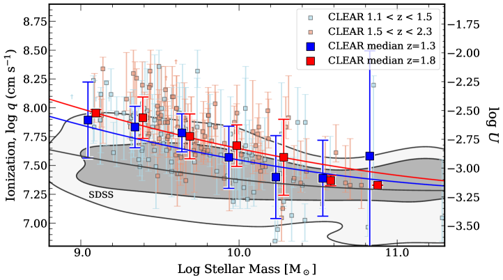
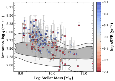
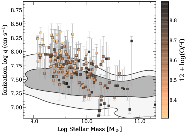
Figure 12: The stellar-mass, ionization relation (MQR) for CLEAR galaxies at $1.1<z<2.3$. The top plot shows the MQR with the CLEAR galaxies color-coded by redshift. Large squares show medians in bins of stellar mass. The error bars show the scatter in each bin. The shaded region denotes the SDSS galaxy distribution of ionization parameters derived using our analysis (identical to that applied to the CLEAR galaxies). The solid lines show analytic fits to the data for the SDSS (black), CLEAR $z=1.3$ (blue), and CLEAR $z=1.8$ samples. The bottom panels show the MQR with galaxies color-coded by specific SFR (bottom left; $\log$ sSFR ) and gas-phase metallicity, $12+\log(\mathrm{O/H})$.

Figure 12 shows the relation between stellar–mass and nebular ionization parameter (i.e., the “mass-ionization-relation”, or MQR) derived for the galaxies in CLEAR at $1.1<z<2.3$. In comparison, we also show the MQR for galaxies in SDSS analyzed using the same set of emission lines and photoionization models used for the analysis of the CLEAR galaxies (see Section 4.2). The MQR clearly evolves from $z\sim 0.2$ (from SDSS) to $z\sim 1.3$ and to $z\sim 1.8$ (from CLEAR). At fixed stellar mass, galaxies have higher ionization parameter at higher redshift, where the effect is stronger for galaxies of lower stellar mass. This extends trends seen both at lower redshift and higher stellar masses (see also Kewley et al. 2015; Kaasinen et al. 2018; Strom et al. 2022).

We parameterize the MQR using a simple quadratic relation inspired by the MZR (Maiolino et al. 2008),

$$\log q=0.0571\times(\log M_{\ast}-\log M_{0})^{2}+\log q_{0}.$$ (6)

Here, $\log M_{0}$ is a scale stellar mass (in units of $M_{\odot}$) when the relation achieves ionization $\log q_{0}$, and $q$ is measured in units of cm s^-1. For our SDSS sample, we fit for $M_{0}$ and $\log q_{0}$. For CLEAR, we fix $\log q_{0}$ to the value derived for the SDSS sample ($\log q_{0}=7.282$) because the stellar-mass distribution of CLEAR peaks at $\log M_{\ast}/M_{\odot}\sim 9.3-9.9$. For CLEAR we also fit $M_{0}$ for galaxies in subsamples of redshift, $1.1<z<1.5$ and $1.5<z<2.3$.

Table 3: Fitted parameters for the analytic form of the mass-ionization relation using Equation 6.

sample	Redshift Range	$\log M_{0}$	$\log q_{0}$
SDSS	$z\sim 0.2$	11.29 $\pm$ 0.11	7.282 $\pm$ 0.007
CLEAR	$1.1<z<1.5$	12.22 $\pm$ 0.10	7.282
CLEAR	$1.5<z<2.3$	12.56 $\pm$ 0.06	7.282

Note. — All fits derived using the nebular ionization parameters derived from the [O ii], [O iii], and H$\beta$ emission lines compared to the MAPPINGS V models.

Table 3 shows the best-fit values and their uncertainties for $M_{0}$ (and $Q_{0}$) for our fits to the SDSS and CLEAR samples. There is a steady increase in $\log M_{0}$ with increasing redshift. This corresponds to an increase in the typical nebular ionization with increasing redshift (at fixed mass). Using these fits, at a stellar mass of $\log M_{\ast}/M_{\odot}=9.0$ we observe an increase in $\log q$ of 0.29 $\pm$ 0.05 dex from $z\sim 0.2$ to $z\sim 1.35$ and an additional increase of 0.14 $\pm$ 0.04 dex from $z\sim 1.3$ to $z\sim 1.8$.

At a stellar mass of $\log M_{\ast}/M_{\odot}=10.0$ the evolution is weaker, as we observe a decrease in ionization parameter of 0.19 $\pm$ 0.03 dex from $z\sim 0.2$ to $z\sim 1.3$. At higher stellar masses $\log M_{\ast}/M_{\odot}\mathrel{\hbox{\hbox to0.0pt{\hbox{\lower 4.0pt\hbox{$\sim$}}\hss}\hbox{$>$}}}10.5$ there is very little evidence that the MQR evolves from $z\sim 0.2$ to $z\sim 1.1-2.3$, but sample is limited by smaller numbers of massive galaxies. For example, Kaasinen et al. (2018) find an increase in the ionization parameter of $\simeq$ 0.3 dex for galaxies with $\log M_{\ast}/M_{\odot}\simeq 10.4-10.9$ from $z\sim 0.2$ to 1.5, only slightly stronger than the trend we see here. Our results are also similar to the independent measurements derived by Strom et al. (2022) at $z\sim 2.3$.

One potential source of concern in the interpretation of the MQR (in Figure 12) is if our sample is biased by sources with strong emission lines. Our samples are selected with $m(\mathrm{F105W})<25$ mag, so sources with strong emission lines could be overrepresented (particularly near our magnitude limit). To test this scenario, we used the measurements of the EW for strong lines ([O ii], H$\beta$, and [O iii]) for sources in our sample (measured from their G102 and G141 spectra) that have redshifts that place these lines in the F105W passband. We then correct the F105W magnitude (using e.g., Eqn. 2 of Papovich et al. 2001), and exclude any object with $m(\mathrm{F105W})>25$ mag. This removes only 9 sources (a loss of $<$5% of the sample). Excluding these 9 sources, we refit the MQR using Equation 6, and find that $\log M_{0}$ is reduced by 0.05 and 0.04 dex for CLEAR at $z\sim 1.3$ and 1.8, respectively (this is less than the statistical uncertainty in Table 3). Therefore, the evolution in the MQR is not seriously impacted by the presence of strong emission lines in the sample.

The bottom panels of Figure 12 show the dependence of the MQR on sSFR and on the gas-phase metallicity. There is a an overall trend of increasing metallicity with increasing stellar mass, which is a consequence of the MZR (see Section 5.1). There is no identifiable trend between metallicity with ionization at fixed mass: for example, galaxies with $\log M_{\ast}/M_{\odot}=9.4-9.8$ span a wide range of $12+\log(\mathrm{O/H})$ and $\log q$. Qualitatively, in this stellar-mass range, galaxies with the highest ionization-parameters have lower metallicity (and vice versa) but this statement is limited by the size of our sample. We return to these points in Section 6.

5.3 Ionization Parameter Dependence on Specific SFR

Another interesting question is to what extent the change in ionization parameter is driven by changes in the SFR (or the changes in SFR at fixed stellar mass, which is the sSFR). Kaasinen et al. (2018) considered the correlation between ionization parameter and sSFR for SDSS galaxies and galaxies at $z\sim 1.5$. They concluded that higher $\log q$ is directly linked to an increase in SFR (see also Brinchmann et al. 2008).

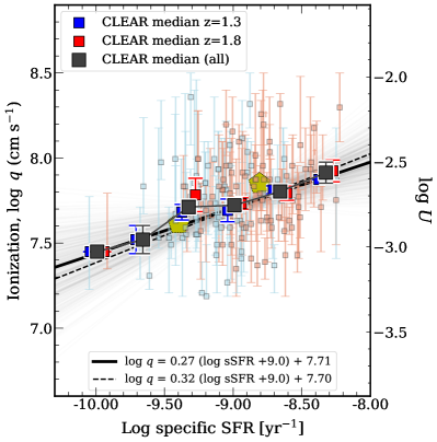
Figure 13: Relation between the specific SFR derived from SED fitting (see Section 2.5) and the gas phase ionization for CLEAR galaxies (see Section 4.2). The right axis shows the equivalent dimensionless ionization parameter, $U\equiv q/c$. The CLEAR galaxies are color coded by redshift; large squares show medians binned by sSFR (error bars show errors on the median). The CLEAR sample includes all galaxies with stellar masses, $\log M/M_{\odot}=[9.2,10.2]$. The dashed line is a linear fit to the CLEAR galaxies. The thick, solid line shows the fit to a subsample with an additional, log sSFR / yr^-1 $>$ $-9.5$ (the light solid lines show 500 random draws from the posterior). The large yellow pentagons show measurements for higher–mass galaxies at $z\sim 1.5$ ($\log M_{\ast}/M_{\odot}=10.4-11$, Kaasinen et al. 2018). There is evidence of a correlation between sSFR and gas ionization. The trend becomes stronger when considering sSFR as traced by the H$\beta$ emission equivalent width (Section 6.4).

To investigate the relation between nebular ionization and sSFR, we focus on CLEAR galaxies in the stellar mass range, $\log M_{\ast}/M_{\odot}=9.2-10.2$ (where the majority of our sample resides). Figure 13 shows the trend between ionization and sSFR for these galaxies in CLEAR. We fit a linear relation,

$$\log q=A\times(\log[\mathrm{sSFR}]+9.0)~{}+~{}\log q_{0},$$ (7)

where $q$ is the ionization parameter (in units of cm s^-1) and the sSFR is estimated from the stellar population fits to the galaxy SEDs (see Section 2.5) in units of yr^-1. Table 4 provides the fitted values and their uncertainties for $A$ and $\log q_{0}$.

In all cases there is a significant correlation between nebular ionization and specific SFR. For fits to the full galaxy sample (not shown in the figure) and for galaxy subsamples, there is a significant correlation (see Table 4). The full galaxy sample gives a slope of $A=0.50\pm 0.10$. We also estimate the significance using Pearson’s correlation coefficient, which gives $r=0.29$ (with a $p$-value of $8.2\times 10^{-5}$ [$3.9\sigma$ for a Gaussian distribution]). Limiting the fit to the subsample of galaxies with stellar mass in the range $\log M_{\ast}/M_{\odot}$ = [9.2, 10.2] yields a weaker correlation coefficient ($r=0.27$), yet still significant ($p=9.2\times 10^{-4}$). Restricting the fit to the subsample with $\log M_{\ast}/M_{\odot}$ = [9.2, 10.2] and $\log$ sSFR / yr^-1 $<-9.5$) yields a correlation coefficient of only $r=0.21$ (with a $p$-value of $0.013$ [about $2.5\sigma$]). While still significant, it is slightly weaker than the relation when considering the full sample, indicating that the range of galaxy stellar masses and/or SFR differences likely account at least partly for the correlation. Kaasinen et al. (2018) also observe a correlation between ionization parameter and sSFR with a very similar slope for measurements from the stacked spectra for $z\sim 1.5$ galaxies at higher stellar masses. Motivated by these results, we explore this relation more below (in Section 6.4).

6 Discussion

In the previous sections we described correlations between strong-line emission-line ratios, gas-phase metallicity ($12+\log(\mathrm{O/H})$), gas ionization parameter ($\log q$), stellar mass and SFR. These trends lead to interesting conclusions about the nature of star-forming galaxies at high redshift, but these depend on the application of the photo-ionization models to the data. In the sections that follow we discuss these factors, and we discuss the implications this makes for the evolution of metallicity and ionization in galaxies.

6.1 Evolution in Mass-Metallicity Relation and Caveats

The evolution in the MZR (Figure 11) has been observed for star-forming galaxies previously, and has been used to constrain the evolution of metals and feedback effects in galaxies as a function of redshift and stellar mass (see, e.g., Maiolino & Mannucci 2019). The most recent measurements find that over the mass range $\log M_{\ast}/M_{\odot}=9.5-10$ the evolution of the gas-phase metallicity evolves by $\Delta\log\mathrm{O/H}$ = 0.2–0.3 dex from $z\sim 2.3$ to $z\sim 0.1$ (e.g., Henry et al. 2021; Sanders et al. 2021). This is generally consistent with our findings in CLEAR, where we see that galaxies at $z=1.35$ (1.90) have metallicity lower by $\Delta\log\mathrm{O/H}$ = 0.25 (0.35) dex compared to SDSS galaxies at $z\sim 0.2$ at stellar masses, $\log M_{\ast}/M_{\odot}=9.4-9.8$.

Some comparisons to other studies of the MZR are useful as they highlight systematics in the analyses. Sanders et al. (2021) studied the evolution of the MZR to $z>3$ using Keck/MOSFIRE observations of $\simeq$450 galaxies. They find that the low-mass slope of the MZR is consistent with no evolution, following $\Delta(\log\mathrm{O/H})/\Delta\log M_{\ast}\sim 0.30$ from $z\sim 0$ to 3.3. However, the normalization of the MZR evolves strongly, with $\Delta(\log\mathrm{O/H})/\Delta z\simeq-0.11$ (at fixed $M_{\ast}$) with a small uncertainty ($\simeq$0.02 dex). They argue this is consistent with the idea that at fixed stellar mass the galaxy gas fractions and metal removal efficiencies increase at higher redshift.

We find stronger evolution with redshift in the normalization in our CLEAR and SDSS samples, $\Delta(\log\mathrm{O/H})/\Delta z=-0.21\pm 0.02$ dex from $z=0.2$ to $z=1.3$ and $\Delta(\log\mathrm{O/H})/\Delta z=-0.34\pm 0.04$ dex from $z=1.35$ to $z=1.90$. This is higher than that from Sanders et al. (2021) by $\sim 0.2-0.3$ dex and is likely related to the use of strong-line metallicity calibrators: Sanders et al. take average metallicities derived from multiple strong-line indicators, while we derive metallicities from the same set of lines fit to the MAPPINGS V photoionization models. Sanders et al. (2021) also use models that allow for increasing $\alpha$/Fe, which could account for some of the offset in the evolution. We take this difference as an estimate of the systematics in the strong-line calibrators (e.g., see Kewley & Ellison 2008, who show the normalization of different calibrators can vary by as much as 0.7 dex).

The study of Henry et al. (2021) is more similar to the analysis presented here. They used measurements from stacked HST/grism spectra of more than 1000 galaxies at $z\sim 1.3-2.3$ (along with higher quality spectra of $\sim$50 individual galaxies) to measure the evolution of the MZR and derived gas metallicities using strong lines ([O ii], H$\beta$, [O iii], H$\alpha$+[N ii]) with the calibration from Curti et al. (2017). They derive O/H abundances at $z\sim 1.3-2.3$ that are consistent with those from Sanders et al. (2018) at $z\sim 2.3$, yielding $\hbox{$12+\log(\mathrm{O/H})$}=8.28\pm 0.02$ ($8.37^{+0.01}_{-0.02}$) for $\log M_{\ast}/M_{\odot}=9-9.5$ ($9.5-10$). Comparing to the $z\sim 0.1$ results from Curti et al. they find that the normalization of the MZR evolves by $\Delta\log\mathrm{O/H}\simeq 0.3$ dex at a fixed mass $\log M_{\ast}/M_{\odot}=9-9.5$. This yields an evolution of $\Delta\log(\mathrm{O/H})/\Delta z\simeq-0.2$ dex from $z\sim 0.1$ to 1.8, consistent with the evolution we derive from our analysis the CLEAR and SDSS samples. The fact that Henry et al. measure the same absolute gas-phase metallicity as Sanders et al. (2018) at $z\sim 2$ but different evolution again indicates that systematics are important, primarily in the absolute normalization of the MZR, both at high and low redshifts.

Table 4: Fitted parameters for the linear relation between specific SFR and nebular ionization for CLEAR galaxies using Equation 7.

sample	slope, $A$	$\log q_{0}$	$r$	$p$-value
Full sample	0.50 $\pm$ 0.10	7.67 $\pm$ 0.02	0.29	8.2$\times$10-5
$\log M_{\ast}/M_{\odot}$=$[9.2,10.2]$	0.31 $\pm$ 0.10	7.70 $\pm$ 0.02	0.27	9.2$\times$10-4
$\log M_{\ast}/M_{\odot}$=$[9.2,10.2]$	0.27 $\pm$ 0.12	7.71 $\pm$ 0.02	0.21	0.013
& $\log\mathrm{sSFR}/\mathrm{yr}^{-1}>-9.5$

In summary, our CLEAR results add to the evidence that the MZR evolves by $\Delta(\log\mathrm{O/H)}/\Delta z\sim 0.2$ dex from $z=0.2$ to $z=1.3$ and that this rate of evolution in the MZR may increase at higher $z$ (we observe $\Delta(\log\mathrm{O/H)}/\Delta z=0.3$ from $z=1.35$ to $z=1.90$). The strength of our result is that we have used the same set of photoionization models to convert the strong emission line ratios to constraints on the gas–phase metallicities and ionization parameters, both for galaxies in CLEAR ($z\sim 1-2.3$) and SDSS (at $z\sim 0.2$). However, this strength is also a weakness because using the same set of photoionization models assumes that the physical conditions in the low redshift galaxies (SDSS) are the same as in the higher-redshift galaxies (CLEAR). For example, we use the MAPPINGS V models with higher pressure, $P_{e}/k=n_{e}T_{e}=10^{6.5}$ cm^-3 K, for the high-redshift galaxies given the expected temperatures and particle density of the H II regions ($T_{e}\sim 10^{4}$ K and $n_{e}\simeq 300$ cm^-3, see Sanders et al. 2016; Kaasinen et al. 2017; Strom et al. 2017; Runco et al. 2021), where the electron density is an order of magnitude larger than observations at $z\sim 0.1$ (e.g., Sanders et al. 2016). As discussed in Kewley et al. (2019b), adopting a lower pressure for the SDSS galaxies would decrease the metallicity of high-$Z$ galaxies at fixed R₂₃. This is evident in Figure 9, which shows difference between our calibration and that from Kewley et al. 2019b (who use $\log P_{e}/k\simeq 5$), and in Appendix A which shows the differences between our MZR and those from Henry et al. (2021, who use the calibration from , which is similar to ). Adopting lower pressure for the SDSS galaxies would lower the metallicity of high-$Z$ galaxies by $\sim 0.1$ dex (see also Sanders et al. 2021). Understanding these potential sources of systematic bias are crucial to have an accurate measurement of the redshift evolution in the MZR.

It is therefore remarkable that even in lieu of the systematic uncertainties, the MZR evolution in Figure 11 shows agreement between measurements from SDSS and CLEAR from different studies Therefore, while there is work needed to understand the impacts of the assumptions about the metallicity calibrations from the strong emission lines, there appears to be some consensus on the absolute evolution of the MZR.

6.2 Evolution in the Mass–Ionization Relation and Caveats

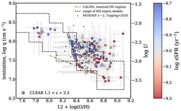
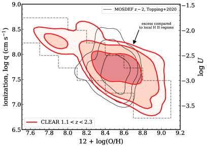
Figure 14: Gas-phase metallicities and ionization parameters for CLEAR galaxies. The top panel shows the data with large squares denoting the CLEAR galaxies (colored by specific SFR). Smaller points show measurements from MOSDEF (Topping et al. 2020). The dashed lines show the range of parameter space covered by nearby H II regions Pérez-Montero (2014). The thick solid lines shows measurements for resolved H II regions in CALIFA galaxies (Espinosa-Ponce et al. 2022). The The right axis shows the equivalent dimensionless ionization parameter, $U\equiv q/c$. The bottom panel shows the same information with a KDE derived distribution (for both the MOSDEF and CLEAR samples).

Figure 12 shows evidence for evolution in the MQR for star-forming galaxies. We quantify the evolution in the MQR over the redshift range $z\sim 0.2$ to $z\sim 2.3$ using our analysis of the galaxies in CLEAR and SDSS. At fixed stellar mass, $\log M_{\ast}/M_{\odot}=9.6$, the differential evolution between the SDSS galaxies and CLEAR galaxies corresponds to $\Delta\log q/\Delta z\simeq 0.2$ dex from $z\sim 0.2$ to $z\sim 1.9$.

Previous studies have seen evidence for this evolution, primarily in terms of an increase at high redshifts in the strength of emission-line ratios that are sensitive to the ionization parameter. Sanders et al. (2018) measured the evolution of O₃₂ as a function of stellar mass and redshift, finding a $0.5$ dex evolution in O₃₂ from $z\sim 2.3$ to $\sim 0$ for galaxies at $\log M_{\ast}/M_{\odot}\simeq\,9.5$. This corresponds to a change in ionization parameter of $\Delta(\log q)\approx 0.4$ dex (using Equation 4). Kaasinen et al. (2018) measured the ionization parameter from stacked spectra of massive galaxies ($\log M_{\ast}/M_{\odot}\simeq 10.4-11$) at $z\sim 1.5$. They showed these exhibit an increase in the ionization parameter of $\simeq$0.4 dex at fixed stellar mass from $z\sim 0.2$ to 1.5. This is consistent with the evolution we measure in CLEAR to $z\simeq 1.9$ and to $z\sim 0.2$ from SDSS.

Figure 12 (bottom-left panel) also shows that at fixed stellar mass galaxies in CLEAR span a range of specific SFR from log sSFR $\sim-9.3$ to $-$8.7, which corresponds to about a factor of $\sim 4$. Qualitatively, the figure shows that galaxies with higher sSFRs favor higher ionization parameters. This is reminiscent of the well-studied trend between the MZR and SFR in that galaxies with lower metallicity favor higher SFRs at fixed stellar mass reported in other studies (see Maiolino & Mannucci 2019; Sanders et al. 2021; Henry et al. 2021).

Is the MQR a consequence of the evolution in the MZR, or of the evolution of the SFR-MZR relation? To investigate this, Figure 12 (bottom-right panel) shows that at fixed stellar mass, higher metallicity galaxies in CLEAR generally have lower ionization parameters, but the scatter is large. The same Figure shows that higher ionization parameters correlate with lower-metallicities. However, we argue the situation is more nuanced: in Section 6.4 we show that galaxies in CLEAR, when matched in stellar mass and metallicity, show a wide range of ionization parameter. Therefore, the metallicity is not solely the cause of the evolution in the MQR.

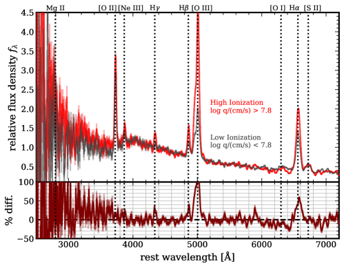
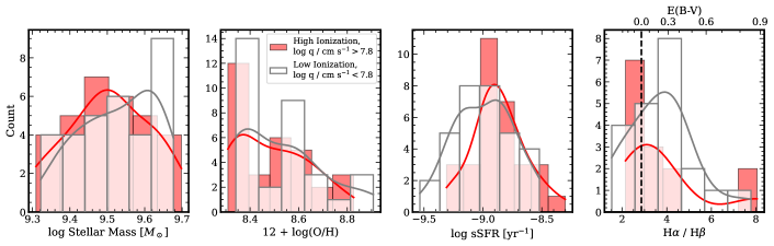
Figure 15: Comparison of the properties of galaxies in the high-ionization subsample ($\log q/[\mathrm{cm~{}s^{-1}}]>7.8)$ compared to the low-ionization subsample ($\log q/[\mathrm{cm~{}s^{-1}}]<7.8)$. The top panel shows the stacked G102 and G141 spectra for each sample (as labeled). Prominent emission features are indicated. All galaxies were selected to have stellar mass $9.3<\log M/M_{\odot}<9.7$ and $12+\log(\mathrm{O/H})>8.3$. The bottom panels show distributions of the galaxy properties in each subsample from this selection, including stellar masses and specific SFRs (derived from SED fitting), the gas-phase metallicities (derived from the emission line analysis), and extinction (derived from the observed H$\alpha$/H$\beta$ ratios). The stellar masses and metallicities are similar between the samples, while the sSFR shows differences (see discussion in the text).

6.3 Evolution of the Gas Metallicity and Ionization

Figure 14 shows the relation between the ionization parameter ($\log q$) and gas–phase metallicity ($12+\log(\mathrm{O/H})$) for the CLEAR galaxies. The figure compares these results to those from MOSDEF (Topping et al. 2020) at $z\sim 2$ and to measurements for individual H II regions in galaxies (Pérez-Montero 2014; Espinosa-Ponce et al. 2022). The metallicity and ionization of the CLEAR galaxies follow the physical parameter space seen in these other samples. Therefore, the general relation between ionization and metallicity seems to describe star-formation in galaxies at both low and high redshifts.

Inspecting Figure 14 more closely, there is also evidence that the distribution of $12+\log(\mathrm{O/H})$ for the $z>1$ galaxies skews to higher ionization parameters at fixed metallicity (at $\hbox{$12+\log(\mathrm{O/H})$}\mathrel{\hbox{\hbox to0.0pt{\hbox{\lower 4.0pt\hbox{$\sim$}}\hss}\hbox{$>$}}}8.4$). This is more apparent in the KDE distributions: compared to the nearby H II regions (compared to both Pérez-Montero 2014 and Espinosa-Ponce et al. 2022). The implication is that galaxies at higher redshift favor higher ionization parameters, (see also Kewley et al. 2015; Strom et al. 2017; Kaasinen et al. 2018; Topping et al. 2020; Runco et al. 2021, see also Sanders et al. 2020 who discuss how a decrease in the effective temperature of stars can lead to an increase in ionization parameter.) Here we see this trend exists for high redshift galaxies even at fixed metallicity and stellar mass.

What causes the increase in ionization parameter? To understand the answer, we divided a sample of galaxies into bins of $\log q$. We selected galaxies at $1.1<z<2.3$ from our CLEAR sample in a narrower range of stellar mass, $9.3\leq\log M_{\ast}/M_{\odot}\leq 9.7$, and we required that the galaxy gas-phase metallicities be $\hbox{$12+\log(\mathrm{O/H})$}>8.3$ (to remove low-metallicity galaxies from consideration). We then divided this sample into a high-ionization subsample of galaxies with $\log q>7.8$ (31 galaxies) and a low-ionization subsample of galaxies with $\log q<7.8$ (32 galaxies). The cuts in stellar mass and ionization have the effect of making both the stellar-mass distribution and metallicity distribution approximately the same for the high– and low–ionization subsamples (see below, and Figure 15). So, we are able to correlate trends between ionization and other galaxy properties.

We then stacked the WFC3 G102 and G141 dust-corrected spectra for these subsamples (following the methods in Section 3.1). Figure 15 shows these stacked spectra for the “low-ionization” ($\log q<7.8$) and “high-ionization” subsamples ($\log q>7.8$). The differences in the spectra are immediately clear (pun intended). The two samples have very different emission-line intensities, while the stellar continua of the two stacks are nearly identical. Figure 15 also shows the relative differences between the two spectra. The strongest difference is in the [O iii] emission, which is nearly twice as strong at the peak of the line for the high-ionization galaxies. The Balmer lines are also stronger by $\approx$30% stronger at the peak of the lines for the high-ionization galaxies. The [O ii] and [Ne iii] lines both show an increase in the higher-ionization subsample, while the [S ii] lines do not.

The bottom row of panels in Figure 15 shows the distributions of stellar mass, gas-phase metallicity, SED-derived sSFR, and the H$\alpha$/H$\beta$ ratios for the high- and low-ionization galaxy subsamples. Both subsamples were selected to have roughly the same stellar mass and gas-phase metallicities, and the panels show there are no substantive differences. Formally, a Kolmogorov-Smirnov (KS) test and a Mann-Whitney-$u$ (MWU) test applied to the distributions return $p$ values of 0.60 and 0.34, respectively, for stellar mass, and 0.45 and 0.71, respectively, for metallicity. However, the specific SFR distributions show evidence they are different. The KS and MWU tests return $p$ values 0.07 and 0.08, respectively. This is apparent in Figure 15 as a shift in the sSFR distribution of the high-ionization subsample toward higher sSFR. The final (right) panel of Figure 15 shows the distribution of the Balmer decrement, but this includes only those galaxies with $z<1.63$ for which H$\alpha$ is detected (14 and 23 galaxies in the high– and low-ionization subsamples, respectively). The mode of the high-ionization subsample is consistent with $E(B-V)=0$, and the low-ionization subsample shows slightly higher attenuation with a mode of $E(B-V)=0.2$, but both have low overall dust attenuation. The KS and MWU tests yield $p$ values of 0.45 and 0.69, respectively, providing no evidence they are drawn from different parent distributions (but this is in part because of the smaller sample sizes).

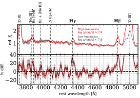
Figure 16: Zoom-in on spectroscopic features in the high-ionization subsample ($\log q/[\mathrm{cm~{}s^{-1}}]>7.8)$ compared to those in the low-ionization subsample ($\log q/[\mathrm{cm~{}s^{-1}}]<7.8)$ from Figure 15. The top panel shows both stacked spectra. The bottom panel shows the percent difference. The H$\beta$ and H$\gamma$ features (labeled in bold) are the most isolated at the resolution of the G102 and G141 grisms (i.e., they are not blended with other possible features). These lines all show excess emission of 20–30% in the high-ionization subsample compared to the low-ionization subsample, This is evidence that higher-ionization galaxies have higher specific SFRs.

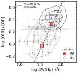
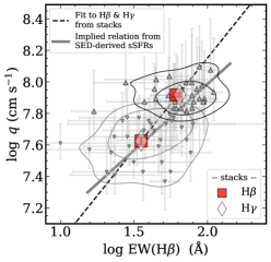
Figure 17: Comparison between H$\beta$ equivalent width, EW, and gas ionization parameter,$\log q$, for CLEAR galaxies in the high-ionization ($\log q>7.8$) and low-ionization subsamples ($\log q<7.8$). The left panel shows the measured [O iii]/[O ii] emission-line ratio against the H$\beta$ equivalent width measured from the stacks (large red squares), and individual points (gray downward / upward triangles show galaxies in the low / high ionization subsamples, respectively). The contours encompass 50 and 84 percentiles for each sample. The other large symbols show values derived from H$\gamma$, scaled by the Case-B ratio to H$\beta$. The dashed line is a linear fit to the stacked measurements. The right panel shows the same distribution against the ionization parameter $\log q$. Because the Balmer emission EW scales with specific SFR, the plots show strong evidence between ionization (and ionization parameter) and specific SFR galaxies at $z\sim 1-2$.

Why then do the galaxies in the high-ionization subsample have such stronger emission lines when all other galaxy properties appear to be similar? The key may be in the fact that see a correlation between these (broad-band-derived) specific SFR and ionization parameters (see Figure 13). Figure 16 shows the region around H$\beta$ and H$\gamma$ in the stacked spectra of the high- and low-ionization subsamples. We focus on these two lines as they are the strongest Balmer emission lines that are unblended at the WFC3 G102 and G141 spectral resolution (e.g., H$\alpha$ is blended with [N ii]; H$\epsilon$ is blended with [Ne III] 3968). Both of these Balmer lines (H$\beta$ and H$\gamma$) are stronger by $\approx$20-30% at the peak of the lines in the high-ionization galaxies.

We measured the strength of these emission lines using pPXF  applied to the stacked spectra (following Section 3.2). Table 1 reports the emission line equivalent widths. For all the Balmer lines, the high-ionization subsample has substantially stronger lines, with the equivalent width of H$\beta$ and H$\gamma$ higher by a factor of $\simeq$1.7–1.9 than those of the low-ionization subsample. Similarly, Figure 17 here shows that correlation between both the Balmer-line equivalent width (EW) against the ionization parameter ($\log q$) and against the [O iii]/[O ii] ratio. In the Figure we show the H$\beta$ EW as it is measured and we have increased the H$\gamma$ EW according to the theoretical H$\beta$/H$\gamma$ Case-B ratio.

The stronger Balmer emission (as evidenced by higher EW) in the high-ionization galaxies indicates that they have a higher production rate of H-ionizing photons (at fixed galaxy stellar mass). This translates to higher specific SFRs: for example, Reddy et al. (2018) show that $\log$ EW(H$\beta$) $=$ $0.32\times\log$ sSFR for galaxies at $z\sim 2$ in MOSDEF. This translates to a factor of two higher sSFR for the high-ionization galaxies in our sample compared to the low-ionization galaxies. We illustrate this in Figure 17, which shows the H$\beta$ EW compared to the both the O₃₂ ratio and the ionization parameter ($\Delta\log q$) in the high-ionization galaxies relative to the low-ionization galaxies. The lines in the Figure show fits,

$$\log\mathrm{O}_{32}=1.4\log\mathrm{EW(H\beta)}-2.3,$$ (8)

$$\log q=1.2\log\mathrm{EW(\hbox{H$\beta$})}+5.8,$$ (9)

for the stacked spectra from the CLEAR subsamples). Using the relation from Reddy et al. (2018), we find that $q\sim\mathrm{sSFR}^{0.4}$ for our CLEAR galaxy samples. Figure 17 also shows how these relations compare to the $\log q$–sSFR (derived from broad-band fitting, see Figure 13, and converted to EW(H$\beta$) using this relation), which is similar. The conclusion is that the ionization parameter and specific SFR are correlated for galaxies at fixed stellar mass and gas-phase metallicity.

Our result for the CLEAR galaxies is consistent with findings from some previous studies. Kewley et al. (2015) show strong evidence that the [O iii]/[O ii] ratio is correlated with the H$\beta$ EW in their sample of $0.2<z<0.6$ galaxies (but they did not differentiate by stellar mass). This is also seen by Kaasinen et al. (2018), who argue that the high ionization parameters for galaxies in their $z<0.3$ sample are driven by the ratio of the number density of hydrogen–ionizing photons to the gas density, and not by (lower) metallicities. In a study of SDSS galaxies, Kashino & Inoue (2019) similarly find that the ionization parameter is predominantly controlled by the specific SFR, with $q\sim\mathrm{sSFR}^{0.43}$ (converting to our units), approximately equal to the relation for the CLEAR galaxies.

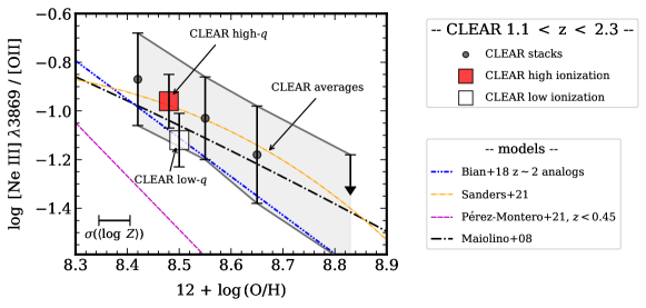
Figure 18: Comparison of [Ne iii]/[O ii] emission line ratios and gas-phase metallicity (12 $+\log$ O/H) derived for CLEAR galaxies and published relations from the literature. The data points show mean metallicities for the CLEAR samples and emission line ratios derived from the stacked spectra. The filled circles show values derived for galaxies in bins of stellar mass (see Section 3). The large squares show values derived for mass-matched samples at high and low ionization ($\log q/[\mathrm{cm~{}s^{-1}}]>7.8$ and $<7.8$, respectively, see Section 6.3), where these is no indication the [Ne iii]/[O ii] ratios are substantially different in these samples (as would be expected if they had significantly different metallicities, see e.g., Sanders et al. 2021). The models also include analogs of $z\sim 2$ galaxies (Bian et al. 2018), calibrations to SDSS at $z\sim 0$ and higher redshifts (Maiolino et al. 2008; Curti et al. 2017; Pérez-Montero et al. 2021).

6.4 Interpretation of the Specific SFR–Ionization Relation at $1.1<z<2.3$

We are now ready to address the question, what is the origin of the correlation between gas ionization parameter ($q$) and specific SFR? First, we consider several explanations for the correlation, including selection and physical effects.

6.4.1 Is a selection effect in stellar mass responsible?

There is an established correlation between stellar mass and ionization (see Figure 12). This is observed in multiple studies, including at high redshift (see, e.g., the recent study of Strom et al. 2022). However, in our analysis the stellar masses of the high-ionization and low-ionization subsamples in Figure 15 are nearly identical (see also the discussion in Section 6.3). We constructed both subsamples to have $9.3<\log M_{\ast}/M_{\odot}<9.7$, where the median stellar masses of both the high and low-ionization samples are both $\langle\log M_{\ast}/M_{\odot}\rangle=9.5$ Figure 15). If the stellar mass was the sole driver, Eq. 6 predicts there should be a difference in the in ionization parameter of only $\Delta\log q$ = 0.03 dex. This is much smaller than the $\Delta\log q\approx 0.3$ dex measured between the two samples (see Figure 13). Therefore, we disfavor stellar mass as the primary driver.

6.4.2 Is a selection effect in gas-phase metallicity responsible?

Figure 14 shows there is a correlation between gas-phase metallicity ($12+\log(\mathrm{O/H})$) and ionization parameter ($\log q$). The distributions of metallicities of the high- and low-ionization are again highly similar (Figure 15, and discussion in Section 6.3). A potential selection effect arises because the $12+\log(\mathrm{O/H})$ values are derived from what surmounts to the O₃₂ and R₂₃ line ratios. R₂₃ is famously double valued, and the fitting method we employed could skew the metallicities to higher values (as the line ratios are unable to get “over the R₂₃ hump” to lower-metallicity values). Indeed, this accounts for the “ridgeline” in the modes of the metallicity–ionization-parameter distributions seen in Figure 14. (This is in essence asking if our modeling prefers the “high-$Z$” solution.)

To test if this potential bias affects the correlation, we used the [Ne iii] $\lambda$3868 / [O ii] ratio an as alternative tracer of gas-phase metallicity. Multiple studies have demonstrated the correlation between [Ne iii]/[O ii] and $12+\log(\mathrm{O/H})$ (e.g., Maiolino et al. 2008; Bian et al. 2018; Pérez-Montero et al. 2021; Sanders et al. 2021). [Ne iii]/[O ii] is particularly useful as the lines are close in wavelength (mitigating extinction effects) and are accessible at rest-frame optical wavelengths. While the [Ne iii] ratio is often too weak to detect in individual galaxies ($\log\hbox{[Ne\,{\sc iii}]}/\hbox{[O\,{\sc ii}]}\sim-1$, see Table 1, although see Backhaus et al. 2022), it is detectable in the stacked spectra.

Figure 15 shows that the [Ne iii]/[O ii] ratios are similar in the stacked spectra of the low- and high-ionization samples. This is supported by the measured [Ne iii]/[O ii] ratios measured from the stacked spectra in Table 1. Figure 18 shows the [Ne iii]/[O ii] against $12+\log(\mathrm{O/H})$ derived from the stacked spectra (compared to the CLEAR stacks for the full sample in bins of stellar mass). Based on the [Ne iii]/[O ii] ratios, there is only a small difference between the values for the high- and low-subsamples ($\log\hbox{[Ne\,{\sc iii}]}/\hbox{[O\,{\sc ii}]}\ \simeq-1.0$ for both), and this is likely attributed to the difference in the ionization (see Kewley et al. 2019b; Maiolino & Mannucci 2019). This is important as the [Ne iii] fluxes are not used in the measurements of $12+\log(\mathrm{O/H})$. Indeed, we measured [Ne iii]/[O ii] in a stacked spectrum of CLEAR galaxies selected to have low metallicity, $12+\log(\mathrm{O/H})$$<$ 8.2, which shows they have much higher ratios, $\log\hbox{[Ne\,{\sc iii}]}/\hbox{[O\,{\sc ii}]}\ \simeq-0.6\pm 0.1$. This is consistent with other studies of low-$Z$ galaxies at these redshifts (e.g., Sanders et al. 2021), and this is substantially higher than that observed in the high- and low-ionization subsamples. Therefore, we disfavor the explanation that metallicity is responsible for the correlation between $\log q$ and sSFR.

6.4.3 Physical connections between the specific SFR and ionization parameter

There are physical reasons to expect a correlation between the specific SFR and the ionization parameter. Such mechanisms need to relate the sSFR (or specifically, the production of ionizing photons per unit mass) to the number density of gas particles. Brinchmann et al. (2008) show this can account for the emission-line ratios of low redshift galaxies (from SDSS, at $z\sim 0.1$). They further argue the elevated ionization parameters result from higher gas densities possibly combined with higher escape fractions of Hydrogen-ionizing photons ($f_{\mathrm{gas}}$). Similar correlations between specific SFR and ionization parameter (and/or line ratios such as [O iii]/[O ii]) have been observed previously at low and high redshifts (e.g., Nakajima & Ouchi 2014; Kewley et al. 2015; Sanders et al. 2016; Bian et al. 2016; Kaasinen et al. 2018; Kashino & Inoue 2019). In our CLEAR sample we see that this correlation persists even when accounting for stellar mass and metallicity (see Figures 13 and 15). Therefore, there is strong evidence for a physical connection between specific SFR and ionization.

A physical connection exists in the case where the H II regions are radiation bounded, where the ionization parameter can be written as (Charlot & Longhetti 2001; Nakajima & Ouchi 2014; Stasińska et al. 2015),

$$q\approx\left(\ \frac{3Q\ n_{\mathrm{H}}\ \epsilon^{2}\ \alpha_{B}^{2}}{4\pi}\ \right)^{1/3},$$ (10)

where $Q$ is the rate of Hydrogen ionizing photons, $\alpha_{B}$ is the case-B Hydrogen recombination coefficient, $n_{\mathrm{H}}$ is the number density of Hydrogen, and $\epsilon$ is the volume filling factor of the gas. At present there is little evidence for changes in $\epsilon$ in any environment (see, Brinchmann et al. 2008), and we do not consider this further here. The ionization parameter therefore depends on $Q$ and $n_{H}$, which observations show are higher at higher redshift (for the case of $n_{H}$; see e.g., Sanders et al. 2016 and Strom et al. 2017) or are expected to be higher at higher redshift (for the case of $Q$, given the observed bluer colors and lower metallicities of galaxies; see, e.g., Shivaei et al. 2018). This is a major driver of the evolution in the MQR (Fig. 12). The geometry of H II regions and star-forming nebula in distant galaxies may be more complicated. This could include nebulae that are either “matter bounded” (also called “density bounded”), where the region of ionization (the Strömgren sphere) extends beyond the nebula (see, e.g., Nakajima & Ouchi 2014) and/or there denser clouds with a low covering fraction (e.g., Naidu et al. 2022). We consider these effects in the discussion that follows.

Production rate of ionizing photons. $Q$ depends on the age of the stellar population, metallicity, and relative number of massive stars (typically those with $\mathrel{\hbox{\hbox to0.0pt{\hbox{\lower 4.0pt\hbox{$\sim$}}\hss}\hbox{$>$}}}10~{}\hbox{$M_{\odot}$}$). Therefore, to increase $Q$ requires either an increase in the relative number of massive stars and/or evolution in the properties of the stellar populations. One obvious possibility is that there is a change in the IMF: either an increase in the upper-mass cutoff, or high-mass slope. Currently evidence for such a changes are inconclusive (e.g., Finkelstein et al. 2011; Narayanan & Davé 2013), so we do not consider it further. However, it will remain important to consider for future studies.

Several studies modeling the UV stellar continua and optical emission line strengths have advocated for higher $Q$ values in some star-forming galaxies at both high and low redshifts, particularly when the metallicity of the stellar continuum is low ($Z\sim 0.1~{}\hbox{$Z_{\odot}$}$; e.g., Topping et al. 2020; Berg et al. 2021; Olivier et al. 2021). This may be exacerbated by super-Solar $\alpha$/Fe ratios, which lead to harder ionizing spectra (at fixed O/H). There is growing evidence for increased $\alpha$/Fe in galaxies at $z\sim 2$ (e.g., Steidel et al. 2016; Strom et al. 2018; Shapley et al. 2019; Sanders et al. 2020; Topping et al. 2020; Runco et al. 2021). One limitation of our work is that the MAPPINGS models do not currently provide for variations in $\alpha$/Fe, and it will important to test how this impacts the trends in our dataset. Nevertheless, for this to drive our observations, $\alpha$/Fe would need to vary with sSFR at fixed [O/H], which would itself be an important discovery. Although our current dataset is insufficient at present, this may be testable in the future by simultaneously modeling the rest-UV continuum spectra and measurements of the optical emission lines of galaxies (e.g., Topping et al. 2020; Olivier et al. 2021).

Gas Density. There is considerable evidence that the gas densities of galaxies at $z\sim 2$ are considerably higher than at low redshift (e.g., Shirazi et al. 2014; Sanders et al. 2016; Acharyya et al. 2019; Runco et al. 2021). This been argued to contribute to the elevated emission-line ratios in high-redshift galaxy samples (Brinchmann et al. 2008; Nakajima & Ouchi 2014; Kewley et al. 2019a). For changes in the gas density to account for our observations, these also must correlate with the specific SFR. One physical explanation for such a correlation is an extension of the Kennicutt–Schmidt relation, where the SFR density scales with gas density, $\rho_{\mathrm{SFR}}\sim\rho_{\mathrm{gas}}^{N}$ (see, e.g., Bacchini et al. 2019). The exponent scales from $N=1.4$ (for the classical Kennicutt-Schmidt relation) to 2 depending on timescales over which star-formation occurs (see, Madore 1977; Larson 1981; Kennicutt et al. 2007; Krumholz 2014; Elmegreen 2015; Bolatto et al. 2017; Bacchini et al. 2019). There are observations of galaxies at low redshift that indicate higher O₃₂ ratios for galaxies with smaller sizes (implying higher densities, e.g., Ji & Giavalisco 2022). Regardless, this provides a physical connection between the strength of H-recombination lines (tracing the SFR density) and the ionization parameter (tracing gas density in H II nebula).

A connection between specific SFR and ionization parameter is therefore expected, and borne out in our CLEAR dataset. Testing if the gas density drives this correlation will be feasible using observations of emission lines whose ratios are dependent on gas density. For example, the ratio of the S⁺ emission lines, [S II] $\lambda 6716$/[S II] $\lambda 6731$ varies by a factor of $\sim$2 as the gas density changes from $n_{e}\simeq 10$ to 1000 cm^-3 (Ryden & Pogge 2021). Currently, HST/WFC3 grism data have insufficient resolution to deblend [S ii] for galaxies at $z\mathrel{\hbox{\hbox to0.0pt{\hbox{\lower 4.0pt\hbox{$\sim$}}\hss}\hbox{$<$}}}1.5$. However, future spectroscopy at higher spectral resolution would be able to test for density variations directly.

Ionizing Radiation Escape Fractions. Several studies of low-redshift galaxies ($z\mathrel{\hbox{\hbox to0.0pt{\hbox{\lower 4.0pt\hbox{$\sim$}}\hss}\hbox{$<$}}}0.1$) show evidence that the escape fraction H-ionizing photons, $f_{\mathrm{esc}}$, is correlated with the ionization parameter, for example where $f_{\mathrm{esc}}\propto(\mathrm{O}_{32})^{2}$ (Chisholm et al. 2018; Izotov et al. 2018; Ji & Giavalisco 2022). This means that the geometry of the H II regions is likely an important factor, where non-uniform covering fractions and/or “matter-bounded” nebulae can lead to a higher escape fractions, $f_{\mathrm{esc}}>0$ (e.g., Nakajima & Ouchi 2014; Naidu et al. 2022). At a fixed ionization parameter, a non-zero $f_{\mathrm{esc}}$ requires a higher number density of ionizing photons relative to the gas density. Using a suite of simulations, Giammanco et al. (2005) showed that increasing the escape fraction of Hydrogen-ionizing photons from $f_{\mathrm{esc}}$=0 to 0.5 increases $\log q$ by as much as 1 dex. This can be boosted in the case of a “density–” (or “matter–”) bounded nebula, where the O⁺ region in the H II–region is truncated while the O⁺⁺ region, located closer to the ionizing source, is not (e.g., Nakajima & Ouchi 2014). This would lead to a potential correlation between $f_{\mathrm{esc}}$ and [O iii]/[O ii] ratio (see also Brinchmann et al. 2008 and Kashino & Inoue 2019). There is recent evidence for this in the findings of Naidu et al. (2022), who argue that high [O iii]/[O ii] line emission of $z\sim 2$ galaxies corresponds to a short-lived phase where massive stars have cleared sightlines in the nebular gas. This produces a geometry with a smaller covering fraction of dense gas, permitting higher $f_{\mathrm{esc}}$ (and higher [O iii]/[O ii]). As pointed out by Brinchmann et al. (2008, and others above), such an increase in $f_{\mathrm{esc}}$ at higher redshift is an important factor in interpreting the emission-line ratios of high redshift galaxies. There are an increasing number of observations (either direct measurements or inferences) that the escape fraction of H-ionizing photons is higher at high redshift (Vanzella et al. 2016, 2018; de Barros et al. 2016; Shapley et al. 2016; Bian et al. 2017; Ji et al. 2020; Begley et al. 2022), where inferences for reionization require $f_{\mathrm{esc}}\sim 0.1-0.2$ (e.g., Ouchi et al. 2009; Robertson et al. 2013; Bouwens et al. 2015; Ishigaki et al. 2018; Finkelstein et al. 2019).

The fact that we observe a correlation between ionization parameter and specific SFR in our CLEAR galaxies then implies there may be a correlation between specific SFR and $f_{\mathrm{esc}}$. This prediction stems from the fact that the ionization parameter and escape fraction are expected to correlate (Nakajima & Ouchi 2014), and we observe a correlation between specific SFR and $\log q$ (Figure 13) and between H$\beta$ EW and $\log q$ (Figure 17). Brinchmann et al. (2008) speculated that such a correlation could account for offsets in the emission-line ratios of SDSS galaxies (see also Nakajima & Ouchi 2014 and Kashino & Inoue 2019). Currently there are only weak constraints on a correlation between specific SFR or ionization parameter and $f_{\mathrm{esc}}$ at high redshifts, though some recent observations are suggestive (but sample sizes remain small, e.g., Bassett et al. 2019 and Naidu et al. 2022). Future observations of the escape fraction in high-$z$ galaxies like those in our CLEAR sample (either with UV spectroscopy or imaging, see Siana et al. 2010), probing a large range in specific SFR, [O iii]/[O ii] ratio would provide the data to test this directly.

We summarize this section by postulating that multiple effects likely contribute to the correlation between specific SFR and ionization parameter. While the current dataset is insufficient to differentiate these effects, we favor the explanation that both an increase in the gas density ($n_{H}$) and the escape fraction of H-ionizing fractions ($f_{\mathrm{esc}}$) drive the trend in specific SFR and ionization parameter, as these have the strongest physical bases. This will be testable directly with future data.

7 Summary

In this Paper, we have used data from CLEAR, including deep spectroscopy from the HST/WFC3 IR grisms, combined with broad-band photometry, to study the stellar populations, ionization and chemical abundances in a sample of $\simeq$ 200 star-forming galaxies at $z\sim~{}1.1-2.3$. At these redshifts the grisms measure emission from strong nebular lines in the rest-frame optical, including [O ii] $\lambda\lambda$3727, 3729, [O iii] $\lambda\lambda$4959, 5008, and H$\beta$, which are sensitive to physical conditions in the galaxies’ star-forming regions (at $z\mathrel{\hbox{\hbox to0.0pt{\hbox{\lower 4.0pt\hbox{$\sim$}}\hss}\hbox{$<$}}}1.5$ the data also cover H$\alpha$+[N ii] $\lambda\lambda$6549, 6585 and [S ii] $\lambda\lambda$6718, 6732). From the emission-line measurements, we derive constraints on the oxygen abundances ($12+\log(\mathrm{O/H})$) and ionization parameters ($\log q$) of the nebular gas using predictions from updated photoionization models (MAPPINGS V, Kewley et al. 2019a). Our findings can be summarized as follows.

1. The CLEAR galaxies show evolution in the gas-phase metallicity–mass relation (MZR) and ionization–mass relation (MQR) as a function of redshift. Galaxies with lower stellar masses have lower gas-phase metallicities and higher ionization parameters. Compared to low-redshift samples ($z\sim 0.2$) at fixed stellar mass, $\log M_{\ast}/M_{\odot}=9.4-9.8$, the CLEAR galaxies at $z=1.35$ (1.90) have lower metallicity, $\Delta(\log Z)$ = 0.25 (0.35) dex, and higher ionization, $\Delta(\log q)$ = 0.25 (0.35) dex. We provided updated analytic calibrations between O₃₂ and the ionization parameter (Eq. 4), and R₂₃ and metallicity (Eq. 3). We further provide analytic fits for the MZR and MQR at $z=1.3$ and $z=1.8$ (Eq. 5 and Eq. 6). Our measurement of the MZR is consistent with other derivations from the literature (e.g., Henry et al. 2021; Sanders et al. 2021), and motivates future studies of the systematics in calibrations of metallicities from strong-line indicators.

2. We find evidence that the ionization parameter $q/c=U$, is correlated with galaxy specific SFR, where $q\sim\mathrm{sSFR}^{0.4}$, derived from changes in the strength of galaxy H$\beta$ EW, where alternatively $\Delta\log q=1.2\log\mathrm{EW}(\hbox{H$\beta$})$ (see Eq. 7). This persists for galaxies at fixed mass and metallicity implying there is an underlying physical connection (see Fig. 17). We consider multiple physical effects for the origin of this relationship. We conclude that the higher gas ionization parameter is a consequence of increasing gas density, $n_{H}$, (and/or variable gas geometry), combined possibly with an increasing H-ionizing photon escape fraction, $f_{\mathrm{esc}}$, and all of these must increase with specific SFR.

Importantly, this work shows the capabilities that space-based observations using near-IR slitless spectroscopy have for engaging in these kinds of scientific studies. This provides a complementary picture to ground-based telescopes (where the capabilities from space provide improvements in wavelength coverage and stable/uniform flux sensitivity and calibration). Future work will expand these types of studies over vastly larger datasets (in the case of NGRST) and wavelength space (in the case of JWST).

Lastly, the work here has important considerations for observations of galaxies at even higher redshift. There is mounting evidence that galaxies near and into the EoR (e.g., $z\mathrel{\hbox{\hbox to0.0pt{\hbox{\lower 4.0pt\hbox{$\sim$}}\hss}\hbox{$>$}}}6$) have higher specific SFRs (e.g., Salmon et al. 2015; Santini et al. 2017), Balmer emission and [O iii] emission-line ratios (e.g., Smit et al. 2015; Roberts-Borsani et al. 2016; Matthee et al. 2017; Stark et al. 2017; Reddy et al. 2018; Hutchison et al. 2019; Endsley et al. 2021). It seems likely therefore that the physical manifestation between specific SFR and these emission line ratios will be similar in such galaxies and those in our CLEAR data. This will be directly testable with forthcoming observations from JWST.

 

We thank our colleagues on the CLEAR team for their valuable conversations and contributions. We wish to acknowledge Yingjie Cheng, Alison Coil, Alaina Henry, Ryan Sanders, Alice Shapley and Allison Strom for helpful comments, feedback, and suggestions (and clarifications). We also thank the anonymous referee for a helpful report, which greatly improved the quality and clarity of this work. This work is based on data obtained from the Hubble Space Telescope through program number GO-14227. Support for Program number GO-14227 was provided by NASA through a grant from the Space Telescope Science Institute, which is operated by the Association of Universities for Research in Astronomy, Incorporated, under NASA contract NAS5-26555. This work is supported in part by the National Science Foundation through grant AST 1614668. CP thanks Marsha and Ralph Schilling for generous support of this research. VEC acknowledges support from the NASA Headquarters under the Future Investigators in NASA Earth and Space Science and Technology (FINESST) award 19-ASTRO19-0122, as well as support from the Hagler Institute for Advanced Study at Texas A&M University. IJ acknowledges support from NASA under award number 80GSFC21M0002. This work was supported in part by NASA contract NNG16PJ33C, the Studying Cosmic Dawn with WFIRST Science Investigation Team. The authors acknowledge the Texas A&M University Brazos HPC cluster and Texas A&M High Performance Research Computing Resources (HPRC, http://hprc.tamu.edu) that contributed to the research reported here. This work benefited from generous support from the George P. and Cynthia Woods Mitchell Institute for Fundamental Physics and Astronomy at Texas A&M University.

Funding for the Sloan Digital Sky Survey IV has been provided by the Alfred P. Sloan Foundation, the U.S. Department of Energy Office of Science, and the Participating Institutions.

SDSS-IV acknowledges support and resources from the Center for High Performance Computing at the University of Utah. The SDSS website is www.sdss.org.

SDSS-IV is managed by the Astrophysical Research Consortium for the Participating Institutions of the SDSS Collaboration including the Brazilian Participation Group, the Carnegie Institution for Science, Carnegie Mellon University, Center for Astrophysics | Harvard & Smithsonian, the Chilean Participation Group, the French Participation Group, Instituto de Astrofísica de Canarias, The Johns Hopkins University, Kavli Institute for the Physics and Mathematics of the Universe (IPMU) / University of Tokyo, the Korean Participation Group, Lawrence Berkeley National Laboratory, Leibniz Institut für Astrophysik Potsdam (AIP), Max-Planck-Institut für Astronomie (MPIA Heidelberg), Max-Planck-Institut für Astrophysik (MPA Garching), Max-Planck-Institut für Extraterrestrische Physik (MPE), National Astronomical Observatories of China, New Mexico State University, New York University, University of Notre Dame, Observatário Nacional / MCTI, The Ohio State University, Pennsylvania State University, Shanghai Astronomical Observatory, United Kingdom Participation Group, Universidad Nacional Autónoma de México, University of Arizona, University of Colorado Boulder, University of Oxford, University of Portsmouth, University of Utah, University of Virginia, University of Washington, University of Wisconsin, Vanderbilt University, and Yale University.

Appendix A Modeling Gas-Phase Metallicity and Ionization with [O ii], [O iii], H$\beta$, H$\alpha$+[N ii], and [S ii]

In addition to the lines used above in the analysis (i.e., [O ii], H$\beta$, and [O iii]), the WFC3 grism spectra cover H$\alpha$+[N ii] for galaxies in our sample with $z\mathrel{\hbox{\hbox to0.0pt{\hbox{\lower 4.0pt\hbox{$\sim$}}\hss}\hbox{$<$}}}1.6$ and [S ii] to $z\mathrel{\hbox{\hbox to0.0pt{\hbox{\lower 4.0pt\hbox{$\sim$}}\hss}\hbox{$<$}}}1.5$ (where the H$\alpha$ and [N ii]  lines are blended at the resolution of the WFC3 grism data; see Figures 4 and 5). For those galaxies, we consider how including these emission lines, along with [O ii], H$\beta$, and [O iii], impacts the constraints on the galaxy gas-phase metallicities and ionization parameter.

We selected the subsample of 87 galaxies that have spectroscopic coverage of H$\alpha$+[N ii] (selected from the 196 galaxies in the full sample, see Section 2.4). We also include [S ii] emission if the line is present in the data (for galaxies at $z<1.5$). We then repeated our analysis using IZI with the same set of photoionization models (see Section 4.2), but using the full set of emission line fluxes (and uncertainties): [O ii], H$\beta$, [O iii], and H$\alpha$+[N ii] (and [S ii], if present).

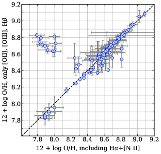
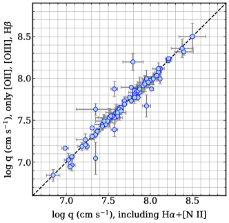
Figure 19: Comparison of gas-phase metallicities (12 + $\log$ O/H) (left) and ionization parameters, $\log q$, (right) derived using [O ii], [O iii], H$\beta$, H$\alpha$+[N ii](which are blended at the resolution of the WFC3 grism) and [S ii] (if present) (on the abscissa), versus fits using only with [O ii], [O iii], H$\beta$ (on the ordinate). The data points show the mode of the metallicity likelihood function, and the error bars show the inter-68-percentile derived from the highest density interval. The dashed line shows the unity relation. The majority of data points have metallicities and ionization parameters that are consistent between the two methods. In a small number of cases (10 out of 87) the metallicities derived including H$\alpha$+[N ii] and [S ii] favor lower gas-phase metallicities. This illustrates that for objects on the lower-branch of the R₂₃ relation additional information may be required to understand their gas phase metallicities.

Figure 19 compares the gas-phase metallicity ($12+\log\mathrm{O/H}$) and ionization parameters ($\log q$) between the values derived using only [O ii], [O iii], and H$\beta$, to those that also include H$\alpha$+[N ii]. The majority of data points show that the results for the ionization parameters from the two methods are nearly unchanged (81/87 $=93\%$ fall on the unity relation within their 68% uncertainties). The metallicities are also mostly consistent between the two methods, where 73/87 $(=84\%)$ fall on the unity relation within their 68% uncertainties. (In both cases the measurements are not independent as they both use some of the same emission lines).

In a small number of cases (10 out of 87) the metallicities derived including H$\alpha$+[N ii] and [S ii] favor significantly lower gas-phase metallicities. Figure 20 shows the posterior likelihoods on the metallicity, $P(12+\log\mathrm{O/H})$ and ionization parameter, $P(\log q)$, for some of these galaxies, comparing the likelihoods derived using only [O ii], [O iii], and H$\beta$, and those that include H$\alpha$+[N ii]. A comparison of the posterior likelihoods show that the constraints on ionization is nearly unchanged. This implies that the ionization is mostly driven by measurements of the [O iii]/[O ii] ratio, and that adding H$\alpha$+[N ii] (and [S ii]) provides little additional information. However, inspection of the metallicity posterior likelihood shows that adding H$\alpha$+[N ii] and [S ii] for some galaxies increases the probably density at lower metallicities. This is akin to stating that these adding H$\alpha$+[N ii] and [S ii] move the metallicity to the “lower branch” of the R₂₃–metallicity relation (see, e.g., Figure 9) and favors lower metallicity solutions as a result. Visually inspecting the spectra and posteriors in Figure 20 we see that in some cases the H$\alpha$ is weakly detected (with lower SNR, e.g., GS 47954 and GS 29256). There are also additional effects, for which our analysis does not account, such as the well-known metallicity (and by proxy, stellar mass) dependence on the [N ii]/H$\alpha$ ratio (e.g., Tremonti et al. 2004; Erb et al. 2006a; Nagao et al. 2006; Kewley et al. 2019b), which may complicate the fitting and interpretation. This illustrates that determining for objects on the lower-branch of the R₂₃ relation additional information may require additional information to understand their gas phase metallicities. Said another way, with CLEAR we are finding that galaxies at $1.1<z<2.3$ with stellar masses around $\log M_{\ast}/M_{\odot}\sim 9.2-10$ have $R_{23}$ values near or approaching the “peak” of the $R_{23}$–metallicity distribution (see figure 9), which occurs at $R_{23}\simeq$1.0 and $12+\log(\mathrm{O/H})\simeq 8.2$ (see equation 3). It is around this inflection point that additional information will be invaluable to diagnosis the metallicities of galaxies.

Figure 20: Examples of galaxies in CLEAR at $1.1<z<1.5$ that have gas-phase metallicities derived using [O ii], [O iii], H$\beta$, H$\alpha$+[N ii], and [S ii] that are substantially lower than those derived using [O ii], [O iii], and H$\beta$ alone. Each row shows one galaxy in our sample (with ID, spectroscopic redshift from the grism data, and stellar mass as indicated). The left panel in each row shows the WFC3 G102 (blue) and G141 (red) 1D extracted spectra. The dashed lines indicate strong emission lines (H$\alpha$ includes [N ii], which is blended at the grism resolution). The middle and right panels show the posterior likelihoods for the gas-phase metallicity, $P(12+\log\mathrm{O/H})$, and ionization parameter, $P(\log q)$, derived using only [O ii], [O iii], and H$\beta$ (shown in tan) compared to those derived using [O ii], [O iii], H$\beta$, H$\alpha$+[N ii], and [S ii] (shown in light blue). The likelihood on the ionization parameters are nearly identical showing these are strongly constrained by [O ii] and [O iii]. The posterior likelihood for metallicity for these galaxies shifts to the “lower branch” of the relation when H$\alpha$+[N ii] and [S ii] are included.

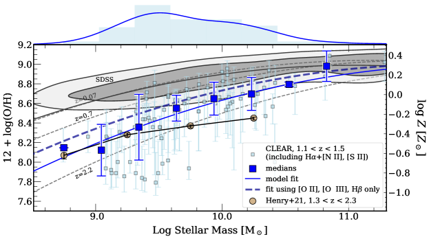
Figure 21: The stellar–mass, gas-phase metallicity relation (MZR) for galaxies at $1.1<z<1.5$ from CLEAR with metallicities derived using the combination of [O ii], [O iii], H$\beta$, H$\alpha$+[N ii], and [S ii]. The small-blue data points show the results for individual galaxies. The large data points show medians in bins of stellar mass. The shaded region shows the distribution derived using the same combination of emission lines from SDSS DR14. The black solid, thin line shows our fit to the SDSS galaxies. The dotted lines show the MZR relation at $z=0.07$, 0.7, and 2.2 from Maiolino et al. (2008). The histogram and curve along the top of the panel shows the distribution of stellar masses for the CLEAR galaxies in this subsample . The solid, thick line shows the fit to the CLEAR galaxies in this subsample; the dashed, thick line shows the fit to these same CLEAR galaxies using the metallicities derived only from [O ii], [O iii], and H$\beta$. The large circles show the relation derived by Henry et al. (2021) using all available emission lines (including data for this sample) with a different calibration of metallicity (see text).

Figure 21 shows the impact on the stellar-mass, gas-phase-metallicity (MZR) relation for galaxies in the CLEAR subsample with $1.1<z<1.5$, that include metallicities derived using the combination of [O ii], [O iii], H$\beta$, H$\alpha$+[N ii], and [S ii]. The figure compares the updated analytic fit (Eq. 5) with $\log M_{0}/M_{\odot}=12.07\pm 0.06$. Therefore, including the H$\alpha$+[N ii] lines shifts the MZR to lower metallicities at fixed stellar mass (compared to results using only [O ii], [O iii], and H$\beta$) of $\Delta\log Z=0.15$ (0.10) dex at a fixed stellar mass of $\log M_{\ast}/M_{\odot}=9.0$ (10.0) at $1.1<z<1.5$, but the overall qualitative trend in the MZR is unchanged from the results above.

Figure 21 also compares the results from CLEAR to those from Henry et al. (2021). These authors combined results from available WFC3 grism data for galaxies at $1.3<z<2.3$ that includes CLEAR along with other datasets (WISPS, Atek et al. 2010; 3DHST, Momcheva et al. 2016). These authors derive gas-phase metallicities calibrated against the relation from Curti et al. (2017). As illustrated in Figure 9, at lower values of metallicity (i.e., $8.0<12+\log\mathrm{O/H}<8.2$) the Curti et al. relation is similar to our results (derived by fitting the photoionization models from MAPPINGS V, Kewley et al. 2019a). However, at higher metallicities (i.e., $12+\log\mathrm{O/H}\mathrel{\hbox{\hbox to0.0pt{\hbox{\lower 4.0pt\hbox{$\sim$}}\hss}\hbox{$>$}}}8.4$) the Curti et al. relation is offset by 0.2–0.3 dex toward lower metallicities. This is evidence in Figure 21 which shows the MZR we derive (including [O ii], [O iii], H$\beta$, H$\alpha$+[N ii]) is consistent with that from Henry et al. for lower stellar masses/metallicities, but we observe an offset to higher metallicity at fixed stellar mass for higher masses/metallicities. The magnitude of this offset consistent with the systematic uncertainties in metallicity calibrations. This highlights the importance of including systematic uncertainties arising from calibration when interpreting the absolute evolution of the mass-metallicity relation.

Appendix B On the Effects of Dust Attenuation

In the analysis above, we have implicitly assumed that the dust attenuation of the nebular gas is equal to that of the stellar continua (see Section 3.1). That is, we take, $E(B-V)_{\mathrm{nebular}}=E(B-V)_{\mathrm{continuum}}$, where $E(B-V)=A(B)-A(V)$ is the color excess. The literature has found varying relationships between $E(B-V)_{\mathrm{gas}}$ (sometimes called $E(B-V)_{\mathrm{nebular}}$) and $E(B-V)_{\mathrm{continuum}}$ (sometimes called $E(B-V)_{\mathrm{stars}}$). Calzetti (2001) discuss the evidence that the nebular gas experiences roughly twice the dust attenuation as the stars in the integrated emission for local UV-luminous galaxies, with $E(B-V)_{\mathrm{nebular}}=E(B-V)_{\mathrm{continuum}}/0.44$. However, galaxies at higher redshifts, $z\sim 2$, show that the attenuation of the gas is more consistent with that of the stars, where $E(B-V)_{\mathrm{nebular}}\approx E(B-V)_{\mathrm{continuum}}$ (Erb et al. 2006b; Reddy et al. 2015), at least for galaxies with relatively low attenuation. For example, Reddy et al. (2015) found that the majority ($>50$%) of objects in their $H$-band selected sample of $z\sim 2$ galaxies (from MOSDEF) are consistent with $E(B-V)_{\mathrm{nebular}}=E(B-V)_{\mathrm{continuum}}$ (within the 1$\sigma$ uncertainties). Reddy et al. also found that the attenuation of the gas increases with respect to that of the stars for galaxies with higher stellar masses and SFRs, where the relation approaches $E(B-V)_{\mathrm{nebular}}=E(B-V)_{\mathrm{continuum}}/0.44$ for galaxies with SFR $>$ 20 $M_{\odot}$ yr^-1. Nearly all galaxies in our CLEAR sample have SFRs below this value: 95% of the sample have SFRs in the range, 2.2 – 19 $M_{\odot}yr^{-1}$ (see Figure 2). Therefore we we have assumed $E(B-V)_{\mathrm{nebular}}=E(B-V)_{\mathrm{stars}}$.

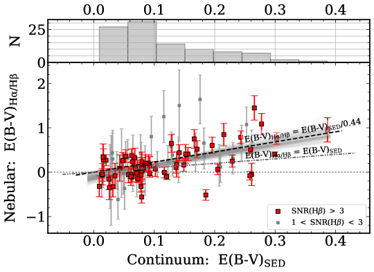
Figure 22: The relation between dust attenuation derived from the SED fitting, $E(B-V)_{\mathrm{SED}}$ and that derived directly from the H$\alpha$/H$\beta$ line ratio, $E(B-V)_{\mathrm{H\alpha/H\beta}}$. This plot shows data for CLEAR galaxies in our sample with $z<1.5$ where both H$\alpha$ and H$\beta$ lines are detected. The figure shows that considering the whole sample the nebular gas (traced by the H$\alpha$/H$\beta$ ratio) experiences more dust attenuation than the stars (traced by the continuum, modeled by the SED fitting). A linear fit (using linmix)to the full sample shows a best fit of $E(B-V)_{\mathrm{H\alpha/H\beta}}=E(B-V)_{\mathrm{SED}}/(0.4\pm 0.2$) (indicated by the swath of gray lines, which show random draws from the posterior of the fit). However, the majority of the galaxies ($>66$%) have $E(B-V)_{\mathrm{SED}}<0.13$, for which the data are consistent with $E(B-V)_{\mathrm{H\alpha/H\beta}}\approx E(B-V)_{\mathrm{SED}}$. We therefore adopt $E(B-V)_{\mathrm{nebular}}=E(B-V)_{\mathrm{SED}}$, but we show in Appendix B that assuming higher dust attenuation for the nebular gas would not impact substantially any of our findings.

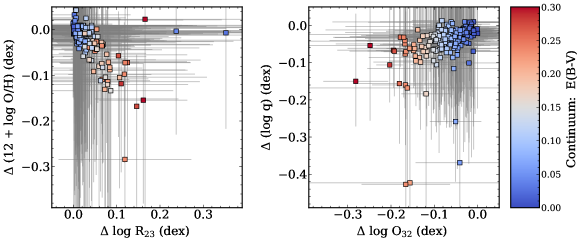
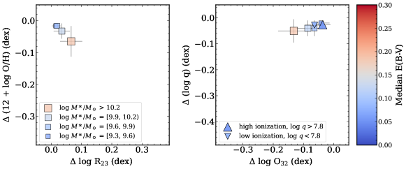
Figure 23: Change in R₂₃ and O₂₃ emission line ratios, and the derived gas-phase metallicity ($\Delta\log\mathrm{O/H}$, and ionization parameter, $Delta\log q$) when increasing the amount of dust attenuation in the gas. Each quantity is $\Delta x=x_{2}-x_{1}$, where $x_{1}$ is the quantity assuming equal dust attenuation in the gas and stars, and $x_{2}$ is the quantify assuming more dust attenuation in the gas (with $E(B-V)_{\mathrm{nebular}}=E(B-V)_{\mathrm{SED}}/0.44$). The top panels show the effects on our full sample, color-coded by $E(B-V)_{\mathrm{SED}}$. The bottom panels show medians for different subsamples (as labeled in the legends). For most of the galaxies in our sample, the increase in R₂₃ corresponds to a decrease in metallicity. Similarly the decrease in O₃₂ corresponds to a decrease in ionization parameter. However, the observed effects are small, particularly in the medians for the samples in the MZR, MQR, and when comparing the ionization parameters of the samples of “high” and “low” ionization (see text and Section 6.4).

We are able to test the relation between $E(B-V)_{\mathrm{nebular}}$ and $E(B-V)_{\mathrm{stars}}$ for galaxies in our sample that are well detected in H$\beta$ (with S/N $>$1) and have redshifts $z<1.5$ such that H$\alpha$ is also present in the data. We can then calculate $E(B-V)_{\mathrm{nebular}}=E(B-V)_{\mathrm{H\alpha/H\beta}}$ directly assuming the lines have an intrinsic ratio of H$\alpha$/H$\beta$ = 2.86 (for Case-B recombination, following, e.g., Nelson et al. 2016). Figure 22 compares this against $E(B-V)_{\mathrm{SED}}$ derived from the SED fitting (which we take as an estimate of $E(B-V)_{\mathrm{stars}}$). The figure shows that for galaxies with low attenuation, $E(B-V)_{\mathrm{SED}}\mathrel{\hbox{\hbox to0.0pt{\hbox{\lower 4.0pt\hbox{$\sim$}}\hss}\hbox{$<$}}}0.15$, there is little difference between $E(B-V)_{\mathrm{H\alpha/H\beta}}$ and $E(B-V)_{\mathrm{SED}}$. For galaxies with higher attenuation, we see that the nebular attenuation is higher than that derived from the SED fitting, approaching the value $E(B-V)_{\mathrm{nebular}}=E(B-V)_{\mathrm{stars}}/0.44$ consistent with (Calzetti 2001; Reddy et al. 2015). Formally, we parameterize the relation as $E(B-V)_{\mathrm{H\alpha/H\beta}}=E(B-V)_{\mathrm{SED}}/\kappa$, where a fit to the entire sample in Figure 22 gives $\kappa=0.4\pm 0.2$. This is consistent with Calzetti (2001). However, most of our sample has low over attenuation, with approximately two-thirds having $E(B-V)_{\mathrm{SED}}<0.13$. For this sample, there is no evidence to support a higher dust attenuation in the gas compared to the stars, where we find $\kappa=0.7\pm 2.0$. The CLEAR sample with $E(B-V)_{\mathrm{SED}}<0.13$ have median SFR of $\simeq 4$ $M_{\odot}$ yr^-1 (with an interquartile range of 2–6 $M_{\odot}$ yr^-1) compared to the sample CLEAR sample with $E(B-V)_{\mathrm{SED}}>0.15$ which has a median SFR = 9 $M_{\odot}$ yr^-1 (and interquartile range of 6–14 $M_{\odot}$ yr^-1). Therefore, our findings for CLEAR seem consistent with Reddy et al. (2015). Because the majority of our sample has low color excess and lower SFRs, we therefore argue that $E(B-V)_{\mathrm{nebular}}=E(B-V)_{\mathrm{SED}}$ is a reasonable assumption.

Nevertheless, we have conducted a study to determine what the impact would be if we instead adopted a higher dust attenuation in the nebular gas, using $E(B-V)_{\mathrm{nebular}}=E(B-V)_{\mathrm{SED}}/0.44$. We have repeated all the analyses assuming this case (including recomputing the gas-phase metallicities and ionization parameters). Figure 23 shows how the derived gas-phase metallicities and ionization parameters are impacted by increasing the dust attenuation, assuming $E(B-V)_{\mathrm{nebular}}=E(B-V)_{\mathrm{SED}}/0.44$. Each panel of the Figure shows the quantities ($x$) as $\Delta x=x_{2}-x_{1}$ where $x_{1}$ is the quantity assuming $E(B-V)_{\mathrm{nebular}}=E(B-V)_{\mathrm{SED}}$ (equal dust attenuation in the gas) and $x_{2}$ is the quantify assuming $E(B-V)_{\mathrm{nebular}}=E(B-V)_{\mathrm{SED}}/0.44$ (more dust attenuation in the gas). The increased dust attenuation has more of an effect on the [O ii] flux, which causes the R₂₃ ratio to increase and the O₃₂ ratio to decrease. The left panels show that on average the R₂₃ values of galaxies decrease by 0.05-0.1 dex, which corresponds to an increase in metallicity of $\Delta\log\mathrm{O/H}=0.02-0.06$ dex. This small change would have a minimal impact on the evolution of the MZR as these offsets are significantly smaller than the evolution we measure (Figure 11 and Section 5.1). Similarly, the O₃₂ values on average decrease by 0.05–0.15 dex, which corresponds to a decrease in the ionization parameter by $\approx$0.05 dex. Again, this imposes minimal impact because this is much smaller than the evolution we observe in the MQR (Figure 12 and Section 5.2). For the subsamples of galaxies with “high” and “low” ionization (at fixed stellar mass, see Figure 17 and Section 6.4), the change is also very minor. Qualitatively, the reason for the minimal impact is because the dust attenuation for these samples is already low. Figure 23 shows the ionization parameters would be increased by $0.02-0.04$ dex if the gas experiences stronger dust attenuation compared to that of the stellar continuum. Therefore, our results are reasonably robust even if the nebular gas for our sample is more attenuated than the derived from the SED fits.

References

- Abolfathi et al. (2018) Abolfathi, B., Aguado, D. S., Aguilar, G., et al. 2018, ApJS, 235, 42
- Acharyya et al. (2019) Acharyya, A., Kewley, L. J., Rigby, J. R., et al. 2019, MNRAS, 488, 5862
- Andrews & Martini (2013) Andrews, B. H., & Martini, P. 2013, ApJ, 765, 140
- Asplund et al. (2009) Asplund, M., Grevesse, N., Sauval, A. J., & Scott, P. 2009, ARA&A, 47, 481
- Astropy Collaboration et al. (2013) Astropy Collaboration, Robitaille, T. P., Tollerud, E. J., et al. 2013, A&A, 558, A33
- Atek et al. (2010) Atek, H., Malkan, M., McCarthy, P., et al. 2010, ApJ, 723, 104
- Bacchini et al. (2019) Bacchini, C., Fraternali, F., Iorio, G., & Pezzulli, G. 2019, A&A, 622, A64
- Backhaus et al. (2022) Backhaus, B. E., Trump, J. R., Cleri, N. J., et al. 2022, ApJ, 926, 161
- Bailer-Jones et al. (2018) Bailer-Jones, C. A. L., Rybizki, J., Fouesneau, M., Mantelet, G., & Andrae, R. 2018, AJ, 156, 58
- Baldwin et al. (1981) Baldwin, J. A., Phillips, M. M., & Terlevich, R. 1981, PASP, 93, 5
- Barro et al. (2019) Barro, G., Pérez-González, P. G., Cava, A., et al. 2019, ApJS, 243, 22
- Bassett et al. (2019) Bassett, R., Ryan-Weber, E. V., Cooke, J., et al. 2019, MNRAS, 483, 5223
- Begley et al. (2022) Begley, R., Cullen, F., McLure, R. J., et al. 2022, MNRAS, in press, arXiv:2202.04088
- Berg et al. (2021) Berg, D. A., Chisholm, J., Erb, D. K., et al. 2021, ApJ, 922, 170
- Bergemann et al. (2014) Bergemann, M., Ruchti, G. R., Serenelli, A., et al. 2014, A&A, 565, A89
- Bian et al. (2017) Bian, F., Fan, X., McGreer, I., Cai, Z., & Jiang, L. 2017, ApJ, 837, L12
- Bian et al. (2018) Bian, F., Kewley, L. J., & Dopita, M. A. 2018, ApJ, 859, 175
- Bian et al. (2016) Bian, F., Kewley, L. J., Dopita, M. A., & Juneau, S. 2016, ApJ, 822, 62
- Bian et al. (2010) Bian, F., Fan, X., Bechtold, J., et al. 2010, ApJ, 725, 1877
- Blanc et al. (2015) Blanc, G. A., Kewley, L., Vogt, F. P. A., & Dopita, M. A. 2015, ApJ, 798, 99
- Bolatto et al. (2017) Bolatto, A. D., Wong, T., Utomo, D., et al. 2017, ApJ, 846, 159
- Bouwens et al. (2015) Bouwens, R. J., Illingworth, G. D., Oesch, P. A., et al. 2015, ApJ, 811, 140
- Brammer (2021) Brammer, G. 2021, eazy-py, v0.5.2, Zenodo, doi:10.5281/zenodo.5012705. https://github.com/gbrammer/eazy-py
- Brammer (2022) —. 2022, grizli, v1.5.0, Zenodo, doi:10.5281/zenodo.1146904. https://github.com/gbrammer/grizli
- Brammer et al. (2015) Brammer, G., Ryan, R., & Pirzkal, N. 2015, Source-dependent master sky images for the WFC3/IR grisms, Space Telescope WFC Instrument Science Report, ,
- Brammer et al. (2008) Brammer, G. B., van Dokkum, P. G., & Coppi, P. 2008, ApJ, 686, 1503
- Brammer et al. (2012) Brammer, G. B., van Dokkum, P. G., Franx, M., et al. 2012, ApJS, 200, 13
- Brinchmann et al. (2008) Brinchmann, J., Pettini, M., & Charlot, S. 2008, MNRAS, 385, 769
- Bruzual & Charlot (2003) Bruzual, G., & Charlot, S. 2003, MNRAS, 344, 1000
- Calzetti (2001) Calzetti, D. 2001, PASP, 113, 1449
- Calzetti et al. (2000) Calzetti, D., Armus, L., Bohlin, R. C., et al. 2000, ApJ, 533, 682
- Cappellari (2017) Cappellari, M. 2017, MNRAS, 466, 798
- Charlot & Longhetti (2001) Charlot, S., & Longhetti, M. 2001, MNRAS, 323, 887
- Chen et al. (2012) Chen, Y.-M., Kauffmann, G., Tremonti, C. A., et al. 2012, MNRAS, 421, 314
- Chisholm et al. (2018) Chisholm, J., Gazagnes, S., Schaerer, D., et al. 2018, A&A, 616, A30
- Cleri et al. (2022) Cleri, N. J., Trump, J. R., Backhaus, B. E., et al. 2022, ApJ, 929, 3
- Coil et al. (2015) Coil, A. L., Aird, J., Reddy, N., et al. 2015, ApJ, 801, 35
- Conroy & Gunn (2010a) Conroy, C., & Gunn, J. E. 2010a, FSPS: Flexible Stellar Population Synthesis, , , ascl:1010.043
- Conroy & Gunn (2010b) —. 2010b, ApJ, 712, 833
- Cresci et al. (2019) Cresci, G., Mannucci, F., & Curti, M. 2019, A&A, 627, A42
- Curti et al. (2017) Curti, M., Cresci, G., Mannucci, F., et al. 2017, MNRAS, 465, 1384
- Curti et al. (2020) Curti, M., Mannucci, F., Cresci, G., & Maiolino, R. 2020, MNRAS, 491, 944
- D’Agostino et al. (2019) D’Agostino, J. J., Kewley, L. J., Groves, B., et al. 2019, ApJ, 878, 2
- de Barros et al. (2016) de Barros, S., Vanzella, E., Amorín, R., et al. 2016, A&A, 585, A51
- Delgado-Inglada et al. (2014) Delgado-Inglada, G., Morisset, C., & Stasińska, G. 2014, MNRAS, 440, 536
- Dopita et al. (2013) Dopita, M. A., Sutherland, R. S., Nicholls, D. C., Kewley, L. J., & Vogt, F. P. A. 2013, ApJS, 208, 10
- Ellison et al. (2008) Ellison, S. L., Patton, D. R., Simard, L., & McConnachie, A. W. 2008, ApJ, 672, L107
- Elmegreen (2015) Elmegreen, B. G. 2015, ApJ, 814, L30
- Endsley et al. (2021) Endsley, R., Stark, D. P., Chevallard, J., & Charlot, S. 2021, MNRAS, 500, 5229
- Erb et al. (2006a) Erb, D. K., Shapley, A. E., Pettini, M., et al. 2006a, ApJ, 644, 813
- Erb et al. (2006b) Erb, D. K., Steidel, C. C., Shapley, A. E., et al. 2006b, ApJ, 647, 128
- Espinosa-Ponce et al. (2022) Espinosa-Ponce, C., Sánchez, S. F., Morisset, C., et al. 2022, MNRAS, 512, 3436
- Estrada-Carpenter et al. (2019) Estrada-Carpenter, V., Papovich, C., Momcheva, I., et al. 2019, ApJ, 870, 133
- Estrada-Carpenter et al. (2020) —. 2020, ApJ, 898, 171
- Estrada-Carpenter et al. (2022) —. 2022, ApJ, in prep
- Finkelstein et al. (2011) Finkelstein, K. D., Papovich, C., Finkelstein, S. L., et al. 2011, ApJ, 742, 108
- Finkelstein et al. (2019) Finkelstein, S. L., D’Aloisio, A., Paardekooper, J.-P., et al. 2019, ApJ, 879, 36
- Fioc & Rocca-Volmerange (1999) Fioc, M., & Rocca-Volmerange, B. 1999, arXiv e-prints, astro
- Garg et al. (2022) Garg, P., Narayanan, D., Byler, N., et al. 2022, ApJ, 926, 80
- Giammanco et al. (2005) Giammanco, C., Beckman, J. E., & Cedrés, B. 2005, A&A, 438, 599
- Grogin et al. (2011) Grogin, N. A., Kocevski, D. D., Faber, S. M., et al. 2011, ApJS, 197, 35
- Hainline et al. (2009) Hainline, K. N., Shapley, A. E., Kornei, K. A., et al. 2009, ApJ, 701, 52
- Henry et al. (2013) Henry, A., Scarlata, C., Domínguez, A., et al. 2013, ApJ, 776, L27
- Henry et al. (2021) Henry, A., Rafelski, M., Sunnquist, B., et al. 2021, ApJ, 919, 143
- Hillier & Miller (1998) Hillier, D. J., & Miller, D. L. 1998, ApJ, 496, 407
- Hutchison et al. (2019) Hutchison, T. A., Papovich, C., Finkelstein, S. L., et al. 2019, ApJ, 879, 70
- Ishigaki et al. (2018) Ishigaki, M., Kawamata, R., Ouchi, M., et al. 2018, ApJ, 854, 73
- Izotov et al. (2018) Izotov, Y. I., Schaerer, D., Worseck, G., et al. 2018, MNRAS, 474, 4514
- Ji & Giavalisco (2022) Ji, Z., & Giavalisco, M. 2022, in prep
- Ji et al. (2020) Ji, Z., Giavalisco, M., Vanzella, E., et al. 2020, ApJ, 888, 109
- Jin et al. (2022) Jin, Y., Kewley, L. J., & Sutherland, R. 2022, ApJ, 927, 37
- Juneau et al. (2014) Juneau, S., Bournaud, F., Charlot, S., et al. 2014, ApJ, 788, 88
- Jung et al. (2021) Jung, I., Papovich, C., Finkelstein, S. L., et al. 2021, ApJ, submitted, arXiv:2111.14863
- Kaasinen et al. (2017) Kaasinen, M., Bian, F., Groves, B., Kewley, L. J., & Gupta, A. 2017, MNRAS, 465, 3220
- Kaasinen et al. (2018) Kaasinen, M., Kewley, L., Bian, F., et al. 2018, MNRAS, 477, 5568
- Kashino & Inoue (2019) Kashino, D., & Inoue, A. K. 2019, MNRAS, 486, 1053
- Kelly (2007) Kelly, B. C. 2007, ApJ, 665, 1489
- Kennicutt & Evans (2012) Kennicutt, R. C., & Evans, N. J. 2012, ARA&A, 50, 531
- Kennicutt (1998) Kennicutt, Jr., R. C. 1998, ARA&A, 36, 189
- Kennicutt et al. (2007) Kennicutt, Jr., R. C., Calzetti, D., Walter, F., et al. 2007, ApJ, 671, 333
- Kewley & Dopita (2002) Kewley, L. J., & Dopita, M. A. 2002, ApJS, 142, 35
- Kewley et al. (2013) Kewley, L. J., Dopita, M. A., Leitherer, C. l., et al. 2013, ApJ, 774, 100
- Kewley & Ellison (2008) Kewley, L. J., & Ellison, S. L. 2008, ApJ, 681, 1183
- Kewley et al. (2019a) Kewley, L. J., Nicholls, D. C., Sutherland, R., et al. 2019a, ApJ, 880, 16
- Kewley et al. (2019b) Kewley, L. J., Nicholls, D. C., & Sutherland, R. S. 2019b, ARA&A, 57, 511
- Kewley et al. (2015) Kewley, L. J., Zahid, H. J., Geller, M. J., et al. 2015, ApJ, 812, L20
- Koekemoer et al. (2011) Koekemoer, A. M., Faber, S. M., Ferguson, H. C., et al. 2011, ApJS, 197, 36
- Kriek et al. (2015) Kriek, M., Shapley, A. E., Reddy, N. A., et al. 2015, ApJS, 218, 15
- Kroupa (2001) Kroupa, P. 2001, MNRAS, 322, 231
- Krumholz (2014) Krumholz, M. R. 2014, Phys. Rep., 539, 49
- Larson (1981) Larson, R. B. 1981, MNRAS, 194, 809
- Leitherer et al. (2014) Leitherer, C., Ekström, S., Meynet, G., et al. 2014, ApJS, 212, 14
- Leja et al. (2019) Leja, J., Johnson, B. D., Conroy, C., et al. 2019, ApJ, 877, 140
- Luo et al. (2017) Luo, B., Brandt, W. N., Xue, Y. Q., et al. 2017, ApJS, 228, 2
- Ly et al. (2016) Ly, C., Malkan, M. A., Rigby, J. R., & Nagao, T. 2016, ApJ, 828, 67
- Ly et al. (2015) Ly, C., Rigby, J. R., Cooper, M., & Yan, R. 2015, ApJ, 805, 45
- Madau & Dickinson (2014) Madau, P., & Dickinson, M. 2014, ARA&A, 52, 415
- Madore (1977) Madore, B. F. 1977, MNRAS, 178, 1
- Maiolino & Mannucci (2019) Maiolino, R., & Mannucci, F. 2019, A&A Rev., 27, 3
- Maiolino et al. (2008) Maiolino, R., Nagao, T., Grazian, A., et al. 2008, A&A, 488, 463
- Mannucci et al. (2010) Mannucci, F., Cresci, G., Maiolino, R., Marconi, A., & Gnerucci, A. 2010, MNRAS, 408, 2115
- Matharu (2022) Matharu, J. 2022, ApJ, in prep
- Matthee et al. (2017) Matthee, J., Sobral, D., Darvish, B., et al. 2017, MNRAS, 472, 772
- Momcheva et al. (2016) Momcheva, I. G., Brammer, G. B., van Dokkum, P. G., et al. 2016, ApJS, 225, 27
- Moustakas et al. (2010) Moustakas, J., Kennicutt, Robert C., J., Tremonti, C. A., et al. 2010, ApJS, 190, 233
- Nagao et al. (2006) Nagao, T., Maiolino, R., & Marconi, A. 2006, A&A, 459, 85
- Naidu et al. (2022) Naidu, R. P., Matthee, J., Oesch, P. A., et al. 2022, MNRAS, 510, 4582
- Nakajima & Ouchi (2014) Nakajima, K., & Ouchi, M. 2014, MNRAS, 442, 900
- Narayanan & Davé (2013) Narayanan, D., & Davé, R. 2013, MNRAS, 436, 2892
- Nelson et al. (2016) Nelson, E. J., van Dokkum, P. G., Momcheva, I. G., et al. 2016, ApJ, 817, L9
- Nicholls et al. (2017) Nicholls, D. C., Sutherland, R. S., Dopita, M. A., Kewley, L. J., & Groves, B. A. 2017, MNRAS, 466, 4403
- Oke & Gunn (1983) Oke, J. B., & Gunn, J. E. 1983, ApJ, 266, 713
- Olivier et al. (2021) Olivier, G. M., Berg, D. A., Chisholm, J., et al. 2021, ApJ, submitted, arXiv:2109.06725
- Onodera et al. (2016) Onodera, M., Carollo, C. M., Lilly, S., et al. 2016, ApJ, 822, 42
- Osterbrock (1989) Osterbrock, D. E. 1989, Astrophysics of gaseous nebulae and active galactic nuclei
- Ouchi et al. (2009) Ouchi, M., Ono, Y., Egami, E., et al. 2009, ApJ, 696, 1164
- Pandas Development Team (2020) Pandas Development Team, T. 2020, pandas-dev/pandas: Pandas, vlatest, Zenodo, doi:10.5281/zenodo.3509134. https://doi.org/10.5281/zenodo.3509134
- Papovich et al. (2001) Papovich, C., Dickinson, M., & Ferguson, H. C. 2001, ApJ, 559, 620
- Papovich et al. (2015) Papovich, C., Labbé, I., Quadri, R., et al. 2015, ApJ, 803, 26
- Pauldrach et al. (2001) Pauldrach, A. W. A., Hoffmann, T. L., & Lennon, M. 2001, A&A, 375, 161
- Pérez-Montero (2014) Pérez-Montero, E. 2014, MNRAS, 441, 2663
- Pérez-Montero et al. (2021) Pérez-Montero, E., Amorín, R., Sánchez Almeida, J., et al. 2021, arXiv e-prints, arXiv:2103.10464
- Péroux & Howk (2020) Péroux, C., & Howk, J. C. 2020, ARA&A, 58, 363
- Pirzkal et al. (2018) Pirzkal, N., Rothberg, B., Ryan, R. E., et al. 2018, ApJ, 868, 61
- Planck Collaboration et al. (2020) Planck Collaboration, Aghanim, N., Akrami, Y., et al. 2020, A&A, 641, A6
- Poetrodjojo et al. (2018) Poetrodjojo, H., Groves, B., Kewley, L. J., et al. 2018, MNRAS, 479, 5235
- Reddy et al. (2015) Reddy, N. A., Kriek, M., Shapley, A. E., et al. 2015, ApJ, 806, 259
- Reddy et al. (2018) Reddy, N. A., Shapley, A. E., Sanders, R. L., et al. 2018, ApJ, 869, 92
- Riess et al. (2021) Riess, A. G., Yuan, W., Macri, L. M., et al. 2021, arXiv e-prints, arXiv:2112.04510
- Roberts-Borsani et al. (2016) Roberts-Borsani, G. W., Bouwens, R. J., Oesch, P. A., et al. 2016, ApJ, 823, 143
- Robertson et al. (2013) Robertson, B. E., Furlanetto, S. R., Schneider, E., et al. 2013, ApJ, 768, 71
- Runco et al. (2021) Runco, J. N., Shapley, A. E., Sanders, R. L., et al. 2021, MNRAS, 502, 2600
- Ryden & Pogge (2021) Ryden, B., & Pogge, R. W. 2021, Interstellar and Intergalactic Medium (Cambridge University Press), doi:10.1017/9781108781596
- Salmon et al. (2015) Salmon, B., Papovich, C., Finkelstein, S. L., et al. 2015, ApJ, 799, 183
- Sanders et al. (2017) Sanders, R. L., Shapley, A. E., Zhang, K., & Yan, R. 2017, ApJ, 850, 136
- Sanders et al. (2015) Sanders, R. L., Shapley, A. E., Kriek, M., et al. 2015, ApJ, 799, 138
- Sanders et al. (2016) —. 2016, ApJ, 816, 23
- Sanders et al. (2018) —. 2018, ApJ, 858, 99
- Sanders et al. (2020) Sanders, R. L., Shapley, A. E., Reddy, N. A., et al. 2020, MNRAS, 491, 1427
- Sanders et al. (2021) Sanders, R. L., Shapley, A. E., Jones, T., et al. 2021, ApJ, 914, 19
- Santini et al. (2017) Santini, P., Fontana, A., Castellano, M., et al. 2017, ApJ, 847, 76
- Savaglio et al. (2005) Savaglio, S., Glazebrook, K., Le Borgne, D., et al. 2005, ApJ, 635, 260
- Shapley et al. (2016) Shapley, A. E., Steidel, C. C., Strom, A. L., et al. 2016, ApJ, 826, L24
- Shapley et al. (2015) Shapley, A. E., Reddy, N. A., Kriek, M., et al. 2015, ApJ, 801, 88
- Shapley et al. (2019) Shapley, A. E., Sanders, R. L., Shao, P., et al. 2019, ApJ, 881, L35
- Shirazi et al. (2014) Shirazi, M., Vegetti, S., Nesvadba, N., et al. 2014, MNRAS, 440, 2201
- Shivaei et al. (2015) Shivaei, I., Reddy, N. A., Shapley, A. E., et al. 2015, ApJ, 815, 98
- Shivaei et al. (2018) Shivaei, I., Reddy, N. A., Siana, B., et al. 2018, ApJ, 855, 42
- Siana et al. (2010) Siana, B., Teplitz, H. I., Ferguson, H. C., et al. 2010, ApJ, 723, 241
- Simons et al. (2021) Simons, R. C., Papovich, C., Momcheva, I., et al. 2021, ApJ, 923, 203
- Skelton et al. (2014) Skelton, R. E., Whitaker, K. E., Momcheva, I. G., et al. 2014, ApJS, 214, 24
- Smit et al. (2015) Smit, R., Bouwens, R. J., Franx, M., et al. 2015, ApJ, 801, 122
- Smith et al. (2006) Smith, L. J., Westmoquette, M. S., Gallagher, J. S., et al. 2006, MNRAS, 370, 513
- Somerville & Davé (2015) Somerville, R. S., & Davé, R. 2015, ARA&A, 53, 51
- Stark et al. (2017) Stark, D. P., Ellis, R. S., Charlot, S., et al. 2017, MNRAS, 464, 469
- Stasińska et al. (2015) Stasińska, G., Izotov, Y., Morisset, C., & Guseva, N. 2015, A&A, 576, A83
- Steidel et al. (2016) Steidel, C. C., Strom, A. L., Pettini, M., et al. 2016, ApJ, 826, 159
- Steidel et al. (2014) Steidel, C. C., Rudie, G. C., Strom, A. L., et al. 2014, ApJ, 795, 165
- Straughn et al. (2011) Straughn, A. N., Kuntschner, H., Kümmel, M., et al. 2011, AJ, 141, 14
- Strom et al. (2022) Strom, A. L., Rudie, G. C., Steidel, C. C., & Trainor, R. F. 2022, ApJ, 925, 116
- Strom et al. (2018) Strom, A. L., Steidel, C. C., Rudie, G. C., Trainor, R. F., & Pettini, M. 2018, ApJ, 868, 117
- Strom et al. (2017) Strom, A. L., Steidel, C. C., Rudie, G. C., et al. 2017, ApJ, 836, 164
- Suzuki et al. (2017) Suzuki, T. L., Kodama, T., Onodera, M., et al. 2017, ApJ, 849, 39
- Thomas et al. (2013) Thomas, D., Steele, O., Maraston, C., et al. 2013, MNRAS, 431, 1383
- Topping et al. (2020) Topping, M. W., Shapley, A. E., Reddy, N. A., et al. 2020, MNRAS, 495, 4430
- Tremonti et al. (2004) Tremonti, C. A., Heckman, T. M., Kauffmann, G., et al. 2004, ApJ, 613, 898
- Tumlinson et al. (2017) Tumlinson, J., Peeples, M. S., & Werk, J. K. 2017, ARA&A, 55, 389
- van der Walt et al. (2011) van der Walt, S., Colbert, S. C., & Varoquaux, G. 2011, Computing in Science and Engineering, 13, 22
- Vanzella et al. (2016) Vanzella, E., de Barros, S., Vasei, K., et al. 2016, ApJ, 825, 41
- Vanzella et al. (2018) Vanzella, E., Nonino, M., Cupani, G., et al. 2018, MNRAS, 476, L15
- Virtanen et al. (2020) Virtanen, P., Gommers, R., Oliphant, T. E., et al. 2020, Nature Methods, 17, 261
- Waskom (2021) Waskom, M. L. 2021, Journal of Open Source Software, 6, 3021. https://doi.org/10.21105/joss.03021
- Wisnioski et al. (2015) Wisnioski, E., Förster Schreiber, N. M., Wuyts, S., et al. 2015, ApJ, 799, 209
- Xue et al. (2011) Xue, Y. Q., Luo, B., Brandt, W. N., et al. 2011, ApJS, 195, 10
- York et al. (2000) York, D. G., Adelman, J., Anderson, John E., J., et al. 2000, AJ, 120, 1579
- Zahid et al. (2017) Zahid, H. J., Kudritzki, R.-P., Conroy, C., Andrews, B., & Ho, I. T. 2017, ApJ, 847, 18
- Zahid et al. (2014) Zahid, H. J., Kashino, D., Silverman, J. D., et al. 2014, ApJ, 792, 75