Bias and Priors in Machine Learning Calibrations for High Energy Physics
Abstract
Machine learning offers an exciting opportunity to improve the calibration of nearly all reconstructed objects in high-energy physics detectors. However, machine learning approaches often depend on the spectra of examples used during training, an issue known as prior dependence. This is an undesirable property of a calibration, which needs to be applicable in a variety of environments. The purpose of this paper is to explicitly highlight the prior dependence of some-machine learning-based calibration strategies. We demonstrate how some recent proposals for both simulation-based and data-based calibrations inherit properties of the sample used for training, which can result in biases for downstream analyses. In the case of simulation-based calibration, we argue that our recently proposed Gaussian Ansatz approach can avoid some of the pitfalls of prior dependence, whereas prior-independent data-based calibration remains an open problem.
I Introduction
Calibration is the task of removing bias from an inference – that is, to ensure the inference is “correct on average”. There are two major classes of calibration: simulation-based calibration, where the goal is to infer a truth reference object, and data-based calibration, where the goal is to match simulation and data distributions.
Both simulation-based calibrations and data-based calibrations are essential components of the experimental program in high-energy physics (HEP), and a significant amount of time is spent deriving these results to enable downstream analyses. We focus on the ATLAS and CMS experiments at the Large Hadron Collider (LHC) for our examples, but this discussion is relevant for all of HEP (and really any experiment). ATLAS and CMS have performed many recent calibrations, including the energy calibration of single hadrons Aad et al. (2017); Sirunyan et al. (2017), jets Aad et al. (2021); Khachatryan et al. (2017), muons Aad et al. (2016); Sirunyan et al. (2020a), electrons/photons Aad et al. (2019a); Khachatryan et al. (2015a, b), and leptons Aad et al. (2015); Sirunyan et al. (2018a). The reconstruction efficiencies of all of these objects are also calibrated and include the classification efficiency of jets from heavy flavor Aad et al. (2019b); Sirunyan et al. (2018b) and even more massive particles Aaboud et al. (2019); Sirunyan et al. (2020b).
Machine learning is a promising tool to improve both types of calibration. In particular, machine learning methods can readily process high-dimensional inputs and therefore can incorporate more information to improve the precision and accuracy of a calibration. There have been a large number of proposals for improving the simulation-based calibrations of various object energies, including single hadrons Belayneh et al. (2020); ATLAS Collaboration (2020a); Akchurin, N. and Cowden, C. and Damgov, J. and Hussain, A. and Kunori, S. (2021); Akchurin et al. (2021); Polson et al. (2021); Pata et al. (2021), muons Kieseler et al. (2021), and jets ATLAS Collaboration (2018, 2020b); Sirunyan et al. (2020c); Haake and Loizides (2019); Haake (2020); Baldi, Pierre and Blecher, Lukas and Butter, Anja and Collado, Julian and Howard, Jessica N. and Keilbach, Fabian and Plehn, Tilman and Kasieczka, Gregor and Whiteson, Daniel (2020); Komiske et al. (2017); ATL (2019); Maier et al. (2022); Kasieczka et al. (2020a); Arjona Martínez et al. (2019) at colliders; kinematic reconstruction in deep inelastic scattering Diefenthaler et al. (2021); and neutrino energies in a variety of experiments Liu et al. (2020); Delaquis et al. (2018); Baldi et al. (2019); Abbasi et al. (2021); Aartsen et al. (2020); Carloni et al. (2021). Further ideas can be found in Ref. Feickert and Nachman (2021). For data-based calibration, a machine learning procedure was recently proposed in Ref. Pollard and Windischhofer (2021).
Caution is needed to ensure that calibrations resulting from a machine learning approach satisfy certain important properties. One critical property of a calibration is that it should be universal – a calibration derived in one place should be applicable elsewhere. A non-universal calibration would have a rather limited utility, and can produce undesirable results if applied to a dataset that does not exactly match the calibration dataset. Statistically, universality is synonymous with prior independence. Most of the existing machine-learning-based calibration proposals, though, are inherently prior dependent, as we will explain below.
A second critical property of a calibration is closure, which means that on average, the calibration produces the correct answer.111Any measure of central tendency can be used to measure closure, such as the median or mode. In this paper, we will focus on the mean, as it is the usual target in machine learning and HEP applications. To quantify closure, one often computes the bias of a calibration, which is the average deviation of the calibrated result from the target value. A calibration can be biased due to the choice of estimator or fitting procedure used, even if the usual pitfalls of dataset-induced biases are taken care of. As explained below, universality and closure are related, and a prior-dependent calibration will necessarily have irreducible bias.222Prior independence is a necessary prerequisite for closure. However, even with prior independence, closure is not guaranteed.
In this paper, we explain the origin of prior dependence for common calibration techniques, with explicit illustrative examples, and demonstrate the associated bias that these procedures incur. For simulation-based calibrations, we advocate for our Gaussian Ansatz Gambhir et al. (2022) as a machine-learning-based strategy that is prior independent and bias-free. For data-based calibrations, we are unaware of any prior-independent methods in the literature. We hope that by highlighting these issues, we can inspire the development of prior-independent calibration methods.
The remainder of this paper is organized as follows. In Sec. II, we review the statistical properties of machine-learning-based calibration. In Sec. III, we clarify the meaning of resolution and uncertainty in the HEP context. To demonstrate the issue of prior dependence, we present Gaussian examples in Sec. IV. In Sec. V, we study an HEP application of calibration in the context of jet energy measurements at the LHC. The paper ends in Sec. VI with our conclusions and outlook.
II The Statistics of Calibration
In this section, we review some of the basic features of simulated-based and data-based calibration, and discuss the issues of prior dependence and bias.
II.1 Simulation-based Calibration
In simulation-based calibration, the goal is to infer target (or true) features from detector-level features – that is, to construct an estimator or calibration function where
| (1) |
is the inferred estimate. To carry out simulation-based calibration, one starts with a set of pairs, which typically come from an in-depth numerical simulation of an experiment. For the case study in Sec. V, will be the experimentally measurable features of hadronic jets and will be the true jet energy.
For concreteness, one can think of the calibration function as being parametrized by a universal function approximator such as a neural network, whose weights and biases are learned. This is often done by minimizing the mean squared error (MSE) loss:
| (2) |
where capital letters correspond to random variables and represents the expectation value over the training sample used to derive the calibration. The calibration function is then deployed on the testing sample, which could be the dataset of interest or a hold-out control region.
Using the calculus of variations, one can show that with enough training data, a flexible enough functional parametrization, and a sufficiently exhaustive training procedure, the asymptotic solution to Eq. (2) is:
| (3) |
where lowercase letters correspond to an instance of a random variable. In this way, learns the mean value of for a given in the training set. Alternative loss functions result in statistics other than the mean. See e.g. Ref. Cheong et al. (2020) for alternative approaches, including mode learning, which is a standard target for many traditional calibrations (usually in the form of truncated Gaussian fits; see e.g. Khachatryan et al. (2015b)).
II.2 Prior Dependence and Bias
A key assumption of simulation-based calibration is that the detector response is universal:
| (4) |
This equation says that for a given truth input , the detector response is the same between the training data used for deriving the calibration and the testing data used for deploying the calibration. In some cases, the detector response might depend on more features than , and if these hidden features are mismodeled, then Eq. (4) may not hold. For our analysis of simulation-based calibration, we assume Eq. (4) throughout.
Calibrations of the form of Eq. (3) are not universal, even if the detector response is. Writing out the MSE-based calibration in integral form, we have:
| (5) |
Here, we have used Bayes’ theorem to make explicit the dependence of on , the prior of true values used for the training. Thus, even if is universal via Eq. (4), the truth distribution is not:
| (6) |
The non-universality of the calibration function leads to bias, as we now explain.
The bias of a calibration quantifies the degree of non-closure. Specifically, bias is the average difference between the reconstructed value and the truth reference value. It is evaluated over the test sample, conditioned on the truth values:
| (7) |
A bias of zero means that, on average, the reconstructed and truth values agree. For MSE regression, the bias is:
| (8) | ||||
This bias is dependent on the training prior through . Thus, a prior-dependent calibration is necessarily biased, since it depends on the choice of .333Note that the bias does not depend on the choice of testing prior, , but rather only on . Depending on the choice of , it is possible for the bias to be zero, but this does not imply the inference is prior independent. For example, if , and , then one can show that . Note that even if the training dataset is statistically identical to the testing dataset (i.e. ), it is not guaranteed that the calibration will be unbiased.
One way to reduce the bias is if the prior is “wide and flat enough”, such that the prior asymptotically approaches a uniform sampling over the real line relative to the detector response. For example, one can show using Eq. (8) that if the prior is Gaussian with standard deviation , the detector response is a Gaussian noise model with standard deviation , and the test set is statistically identical to the training set, then the bias scales as:
| (9) |
In cases with steeply falling spectra, as is common in HEP, prior dependence usually leads to large biases in calibration, even if the testing and training sets follow the same distribution.
II.3 Mitigating Prior Dependence
A majority of simulation-based calibrations (with or without machine learning) are set up using the MSE loss as described above, which means that they are biased. That said, there are alternative methods to mitigate the prior dependence and thereby reduce the bias. For example, simulation-based jet calibrations at the LHC use a technique called numerical inversion (see e.g. Ref. Cukierman and Nachman (2017)). The idea of numerical inversion is to regress from with a function and then define the calibration function through the inverse:
| (10) |
Traditionally, is one dimensional and is parametrized with functions that can easily be inverted numerically, hence the name. The function is given by:
| (11) |
Since the detector response is universal, is universal, and thus the derived is also universal. Under certain assumptions, the from numerical inversion is also unbiased Cukierman and Nachman (2017).
Numerical inversion has been extended to work with neural networks ATLAS Collaboration (2018, 2020b), where the inversion step is accomplished with a second neural network. Alternatively, it may be possible to also achieve this with a natively invertible neural network such as a normalizing flow Rezende and Mohamed (2015); Kobyzev et al. (2020). A key challenge with numerical inversion and its neural network generalizations are that they do not scale well to high dimensions.
In Ref. Gambhir et al. (2022), we propose an alternative way to achieve a prior-independent calibration that scales well to high- and variable-dimensional settings. This approach is based on finding the local maximum likelihood, such that the learned calibration function becomes:
| (12) |
where MLC stands for maximum likelihood classifier – see Ref. Nachman and Thaler (2021a). Again, because the detector response is universal, maximum likelihood calibrations are universal,444One important caveat is that universality here means prior independence over the space of priors that share the same support as the training set. One cannot get away with training a model on a single instance and expecting it to work everywhere! and in certain configurations, are provably unbiased. In particular, if the detector response is a Gaussian noise model centered on , then one can show that the bias is zero using Eq. (7):
| (13) | ||||
Here, we have made use of the fact that for a Gaussian, is maximized at , and that the average of this Gaussian is simply . This conclusion holds even if the detector response includes offsets, or if the noise depends on .555It is not always true that a maximum likelihood calibration is unbiased. For instance, if is drawn from a uniform distribution , then the maximum likelihood estimate from a single sample is , whereas an unbiased estimate would be .
The strategy in Ref. Gambhir et al. (2022) is to estimate the (local) likelihood density by extremizing the Donsker-Varadhan representation (DVR) Monroe D. Donsker and S. R. S. Varadhan (1975); Belghazi et al. (2018) of the Kullback-Leibler divergence Kullback and Leibler (1951):
| (14) |
By parametrizing via a specially chosen Gaussian Ansatz (see Ref. Gambhir et al. (2022) for details), one can extract the local maximum likelihood estimate and resolution with a single neural network training.
We focused on regression in the above discussion, but prior dependence also appears in classification calibration. A classifier trained with the MSE loss function or the binary cross entropy (BCE) will learn the probability of the signal given an observed . If the fraction of signal is different in the training set and the test set, that is, , then the output can no longer be interpreted as the probability of the signal. Luckily, classifiers are almost never used this way in HEP, since the classification score is not interpreted directly as a probability.666See Ref. Guo et al. (2017) for a review in the machine learning literature and Ref. Cranmer et al. (2015) for related studies in the context of HEP likelihood ratios. In this case, simulation-based calibrations may not be required,777There may be practical issues associated with prior dependence, e.g., if there is an extreme class imbalance, the classifier may not learn well. In the extreme limit of only one class present in the training, then there is a prior dependence also on the result. though data-based calibrations are still essential, as described next.
II.4 Data-based Calibration
In data-based calibration, the goal is to account for possible differences between a true detector response, and a simulated detector model . That is, the goal is to match detector level features between data and a simulation at the distribution level, in contrast to simulation-based distribution, where the goal is to match and a target feature at the object level. Usually, is a control dataset, and is a simulated detector output generated from truth-level features .
In the machine learning literature, data-based calibration is called domain adaptation. Machine learning domain adaptation has been widely studied in the context of HEP Rogozhnikov (2016); Andreassen and Nachman (2020); Cranmer et al. (2015); Diefenbacher et al. (2020); Nachman and Thaler (2021b) (see also decorrelation Louppe et al. (2017); Dolen et al. (2016); Moult et al. (2018); Stevens and Williams (2013); Shimmin et al. (2017); Bradshaw et al. (2019); ATL (2018); Kasieczka and Shih (2020); Xia (2019); Englert et al. (2019); Wunsch et al. (2019); Rogozhnikov et al. (2015); Collaboration (2020); Clavijo et al. (2020); Kasieczka et al. (2020b); Kitouni et al. (2020); Ghosh and Nachman (2021)), but these tools have not yet been applied to per-object calibrations. Traditional methods typically use binned or simple parametric approaches to calibrate differences between data and simulation.
The authors of Ref. Pollard and Windischhofer (2021) propose to use tools from the field of optimal transport (OT) to perform the data-based calibration using machine learning. The central idea is to learn a map that “moves” as little as possible, but still achieves . In this case, the OT-based calibration is:
| (15) |
where is the Jacobian factor. The precise transportation map depends on the choice of OT metric. Eq. (15) can be interpreted as shifting simulated samples to , and additionally reweighting each sample by . One can also write a corresponding expression for the OT-calibrated detector model, conditioned on :
| (16) |
Eq. (16) can be thought of as a “corrected simulated response” function that accounts for mismodeling in the original simulation, . At first glance, Eq. (16) might seem prior independent, since it is conditioned on the truth-level . As we will see, though, there is implicit prior dependence in . For simplicity, consider the special case of one dimension. Here, for any OT metric, the OT map is simply given by:
| (17) |
where is the cumulative distribution function of , i.e. . This function maps quantiles of the simulated distribution to quantiles of the data distribution. The Jacobian of this transformation is:
| (18) | ||||
Thus, since the prior explicitly appears, the derived OT-based detector model in Eq. (16) is prior dependent.
In line with simulation-based calibration, the bias of a data-based calibration is the average difference between the estimator and the desired value , conditioned on .888This differs from the simulation-based calibration definition, which was conditioned on . In data, there is no truth level . However, sometimes, a proxy can be used as a in data, allowing for a direct comparison of true versus reconstructed values in data-based calibration. For example, when performing data-based calibration on a +jets sample, the of the can be used as a proxy for the true jet . For OT-based calibration, the bias for a given value of is:
| (19) | ||||
If , then the bias is zero. Otherwise, the calibration is biased, a consequence of prior dependence. Note that this is in contrast to simulation-based calibration, where non-universality can imply a bias even if .
II.5 Unbiased Data-based Approaches?
As defined above, the goal of a data-based calibration is to match to . This is an inherently prior dependent task, however, since – that is to say, the simulated detector output depends on the simulation input. Instead, one can ask if the corrected response function, , is universal. If it is, then one can use the same corrected response function to generate for a variety of priors . At least in the special case of one-dimensional OT-based calibration, however, we have shown above that the corrected response function is not universal.
To our knowledge, no one has proposed a data-based calibration method that is prior independent, whether using machine learning or not. This implies that all data-based calibration methods in use are biased, though the degree of bias may be small if the testing and training truth-level densities are similar enough. We encourage the community to develop a prior-independent data-based calibration strategy, or prove that it is impossible.
III Resolution and Uncertainty in Calibrations
The discussion thus far has focused on mitigating bias in calibration. Two related concepts are the resolution and uncertainty of a calibration. In this section, we review calibration resolution and uncertainty, and we clarify important nomenclature in HEP settings.
III.1 Resolution
As already mentioned, the bias of a calibration refers to the difference in central tendency (such as the mean, median, or mode) between a reconstructed quantity and a reference quantity. By contrast, the resolution of a calibration refers to the spread in the difference between the reconstructed and reference quantities. Using variance as our measure of spread, the resolution can be written as the variance of differences between the reconstructed and truth values, conditioned on the truth values, evaluated over the test sample:
| (20) |
Resolutions, like biases, can be prior dependent. When using the MSE-based calibration (Eq. (3)), this becomes:
| (21) | ||||
The prior dependence is seen by applying Bayes’ Theorem to .
As before, this prior dependence can be reduced if the prior is wide compared to the detector response. If the prior is Gaussian with standard deviation , and the detector response is a Gaussian noise model with standard deviation , then by applying Eq. (III.1), one can show that the resolution scales as:
| (22) |
On the other hand, for the prior-independent MLC calibration (Eq. (12)), the resolution can be shown to be:
| (23) |
In HEP (and many other) applications, however, it is common to instead refer to the resolution with respect to a measurement rather than the true value . That is, for an inference , we would like a measure of the spread of values consistent with this measurement, which we will denote (distinguished by the argument rather than ). Depending on the context and type of calibration, there are a variety of ways to define – for instance, as the standard deviation from a Gaussian fit to the distribution of reconstructed over true energies (see e.g. Ref. Cukierman and Nachman (2017)). For our purposes, we can define the point resolution as the variance of ’s conditioned on :
| (24) | ||||
For the MSE-based calibration, this is simply the variance of the posterior, . However, for frequentist approaches where the posterior is not well defined, such as the maximum likelihood calibration, the resolution cannot be defined this way and care must be taken. For Gaussian noise models , the likelihood is symmetric under interchanging the arguments and , so one can take the resolution to be (applying Eq. (20)):
| (25) |
Calibrations do not necessarily improve the resolution and can sometimes make the resolution seem worse. For example, if a calibration requires multiplying the reconstructed quantity by a fixed number greater than one, then the resolution will grow by the same amount.999This is also true if we had used the relative resolution, , which is also commonly used in HEP, rather than the absolute resolution. It is therefore important to compare resolutions only after calibration.
If a calibration incorporates many features that determine the resolution of a given quantity, then the resolution can improve from calibration. For example, suppose the reconstructed value is some function of observable quantities , i.e. . For instance, in the context of jet energy calibrations, for some constant and an observable quantity (e.g. energy dependence on the pseudorapidity). If any of the have a non-trivial probability density, this will be inherited by the reconstructed value and thus will have a non-zero resolution. This resolution is completely reducible, however, through a calibration that is dependent – that is, a calibration function rather than . The ability to incorporate many auxiliary features is why machine-learning-based approaches, such as the Gaussian Ansatz Gambhir et al. (2022), have the potential to improve analyses at HEP experiments.
III.2 Uncertainty
In the machine learning literature, “resolution” would be referred to as a type of “uncertainty”. Uncertainty in the statistical context refers to the limited information about contained in . In the HEP literature, though, we use uncertainty in a different way, to instead refer to the limited information we have about the bias and resolution of a calibration.
The reason for this difference in nomenclature is that HEP research is based primarily on simulation-based inference, where data are analyzed by comparison to model predictions. (This is the case for the vast majority of analyses at the LHC.) In this context, the word “uncertainty” is reserved to refer to uncertainties on model parameters. A worse resolution can degrade the statistical precision of a measurement, but if it is well modeled by the simulation, then there is no associated systematic uncertainty (though there will still be statistical uncertainties).
Both simulation-based and data-based calibrations can have associated uncertainties. For simulation-based calibrations, even if they are prior independent, there can be uncertainties in the detector models themselves. For data-based calibrations, there are additional uncertainties associated with the truth-level prior; see Sec. II.5.
One of the goals of data-based calibration is to improve the modeling of the calibration in simulation to match the data. Typically, data-based calibrations are performed in dedicated event samples with well-understood physics processes. The residual uncertainty following the data-based calibration is dominated by the modeling of the underlying process. For example, data-based jet calibrations (called “in situ” calibrations) compare the jet to a well-measured reference object such as a boson. The momentum imbalance between the jet and the boson will be due in part to differences in the calibration between data and simulation and in part due to the mismodeling of initial and final state radiation. Uncertainties on the latter are then incorporated into the data-based calibration uncertainty. In nearly all cases, data-based calibrations are performed independent of the uncertainties, which are computed post-hoc. In the future, these uncertainties may be improved with uncertainty/inference-aware machine learning methods Blance et al. (2019); Englert et al. (2019); Louppe et al. (2017); Dolen et al. (2016); Moult et al. (2018); Stevens and Williams (2013); Shimmin et al. (2017); Bradshaw et al. (2019); ATL (2018); Kasieczka and Shih (2020); Wunsch et al. (2019); Rogozhnikov et al. (2015); Collaboration (2020); Clavijo et al. (2020); Kasieczka et al. (2020b); Kitouni et al. (2020); Estrade et al. (2019); Wunsch et al. (2020); Elwood et al. (2020); Xia (2019); De Castro and Dorigo (2019); Charnock et al. (2018); Alsing and Wandelt (2019); Simpson and Heinrich (2022); Kasieczka et al. (2020a); Bollweg et al. (2020); Araz and Spannowsky (2021); Bellagente et al. (2021); Nachman (2019); Dorigo and de Castro (2020); Ghosh and Nachman (2021); Ghosh et al. (2021).
IV Gaussian Examples
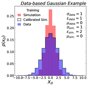
In this section, we demonstrate some of the calibration issues related to bias and prior dependence in a simple Gaussian example. We assume that the truth information (the “prior”) is distributed according to a Gaussian distribution with mean and variance :
| (26) |
The detector response is assumed to induce Gaussian smearing centered on the truth input with variance :
| (27) |
For the simulation-based calibration in Sec. IV.1, the goal is to learn given , assuming perfect knowledge of the detector response. For the data-based calibration in Sec. IV.2, the goal is to map in “simulation” to in “data”. In this latter study, we assume that data and simulation have the same true probability density and differ only in their detector response, – that is, “mismodels” .
IV.1 Simulation-based Calibration
If we use the MSE approach in Eq. (3), there is a prior dependence in the calibration, which induces bias. Perhaps counter-intuitively, this bias persists even if the prior is the same as the data density:
| (28) |
as we now show.
In the Gaussian case, the reconstructed data are distributed according to:
| (29) |
and it is possible to solve Eq. (5) analytically, in the asymptotic limit:
| (30) |
For comparison, we can also compute the unbiased maximum likelihood calibration using Eq. (12):
| (31) |
It is also possible to analytically compute the point resolutions, , for both the MSE and MLC fits (Eqs. (24) and (25), respectively):
| (32) | ||||
| (33) |
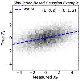
To illustrate this setup, we simulate this scenario numerically for , , and . In Fig. 1a, we show the simulated data, for which both the true and reconstructed values follow a Gaussian distribution. The first step of a typical calibration is to predict the true from the reconstructed . Since we know that the average dependence of the true on the reconstructed is linear, we perform a first-order polynomial fit to the data using numpy polyfit, which is represented by the blue dashed line in Fig. 1a. This calibration function is then applied to all reconstructed values:
| (34) |
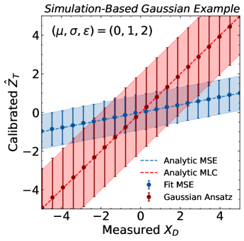
The resulting calibration curve is presented in blue in Fig. 1b, along with the associated resolution .
For comparison, we perform a maximum likelihood calibration using the Gaussian Ansatz introduced in Ref. Gambhir et al. (2022):
| (35) |
where we have dropped the subscripts (, ) for compactness of notation. As described in Ref. Gambhir et al. (2022), the calibration function is obtained by minimizing the DVR loss function from Eq. (14), such that after training:
| (36) | ||||
| (37) |
For Gaussian noise models, this maximum likelihood estimate is unbiased, as confirmed by the numerical results in Fig. 1b. We implement the Gaussian Ansatz in Keras Chollet (2017) with the Tensorflow backend Abadi et al. (2016). The network consists of three hidden layers with 16 nodes per layer, with rectified linear unit activations. The and networks are each a single node with linear activation. The network is set to zero by hand. Optimization is carried out with Adam Kingma and Ba (2014) over 100 epochs with a batch size of 128. As desired, the Gaussian Ansatz yields a calibration that is independent of the prior .
To demonstrate the bias, we plug in Eq. (28) into Eq. (8) to get the bias from the MSE calibration approach:
| (38) |
It is possible to solve Eq. (38) analytically for the Gaussian setup:
| (39) |
As expected, as . For , though, there is a non-zero bias with the MSE approach. The -binned resolutions can also be computed using Eqs. (III.1) and (23):
| (40) | ||||
| (41) |
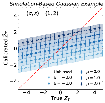
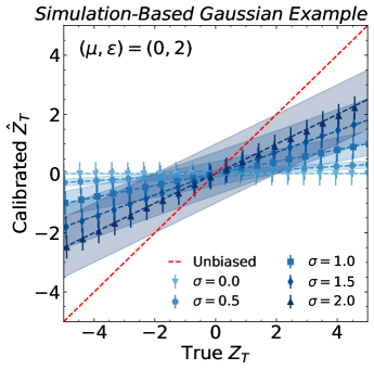
The fitted biases and resolutions are presented in Fig. 2, which exhibits the bias expected from Eq. (39). This illustrates the large bias introduced by the MSE regression procedure.
To further highlight the role of prior dependence, we repeat the MSE calibration procedure, where we test multiple values of the prior parameters and to confirm the predictions in Eq. (39). As shown in Fig. 2a, changes in simply shift the calibration up and down, but do not improve the calibration quality across the true values of . As shown in Fig. 2b, changes in change the slope of the calibration. In the limit , the calibration curve approaches the unbiased curve, as anticipated from Eq. (9).
IV.2 Data-based Calibration
As discussed in Sec. II.5, we are unaware of any prior-independent data-based calibration. To highlight this challenge, we study the OT-based technique introduced in Ref. Pollard and Windischhofer (2021) and mentioned in Sec. II.4. In our Gaussian example, the goal is to calibrate a “simulation” sample with to match a “data” sample with .
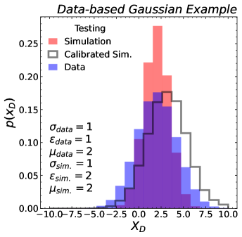
For simplicity, we assume that the true spectra (determined by ) are the same in data and in simulation, such that there is no systematic uncertainty in the calibration (see Sec. III.2). Only , the parameter governing the detector response, is different between simulation and data – the simulation mismodels the real detector. To highlight the issue of prior dependence, we consider a “training” set with one value of and a “testing” set with a different value of , with a shared value of . The calibration will be derived on the training set and deployed on the testing set. Again for simplicity, we assume that detector effects (determined by ) are the same in both the train and test sets.
The one-dimensional OT map from one Gaussian to another Gaussian can be computed analytically:
| (42) |
where the mean and standard deviation of sample are and , respectively. This equation can be derived following Eq. (17), by computing cumulative distribution function (CDF) of sample with the inverse CDF of sample .
For the training set with , we have
| (43) | ||||
The test set only differs in the value of , so the correct calibration function should be:
| (44) | ||||
As long as , then and so the calibration is not universal.
A numerical demonstration of this bias is presented in Fig. 3, where histograms of the data and simulation are presented along with the calibrated result. In Fig. 3a, we see the calibration derived in the training sample, where by construction, the calibrated simulation matches the data. Since the truth distribution is different in the test set, however, the training calibration applied in the test set is biased, as shown in Fig. 3b. The actual calibration function is plotted in Fig. 4 and compared to the analytic expectation from Eqs. (44) and (43). The fact that the calibration derived on the train set is not the same as the calibration derived on the test set shows that the calibration derived in one and applied to the other will lead to a residual bias.
V Calibrating Jet Energy Response
Jets are ubiquitous at the LHC, and their calibration is an essential input to a majority of physics analyses performed by ATLAS and CMS. In this section, we consider a simplified version of simulation-based and data-based jet energy calibrations. To illustrate the impact of the prior dependence, we use a realistic and also extreme example where calibrations are derived in a sample of generic quark and gluon jets and then applied to a test sample of jets from the decay of a heavy new resonance. To further simplify the problem, we consider a calibration of the invariant mass of the leading two jets. In practice, jet energy calibrations are derived for individual jets, but this requires at least including calibrating the jet rapidity in addition to the jet energy. We keep the problem one-dimensional in order to ensure the problem is easy to visualize and to mitigate the dependence on features that are not explicitly modeled. For a high-dimensional study of jet energy calibrations in a prior-independent way, see Ref. Gambhir et al. (2022).
V.1 Datasets
Our study is based on generic dijet production in quantum chromodynamics (QCD). For these studies, we will consider two different datasets to demonstrate simulation-based and data-based jet energy calibrations. The first dataset is made with a full detector simulation. The full simulation sample uses Pythia 6.426 Sjöstrand et al. (2006) with the Z2 tune Chatrchyan et al. (2011) and interfaced with a Geant4-based Agostinelli et al. (2003); Allison et al. (2006, 2016) full simulation of the CMS experiment Chatrchyan et al. (2008). In simulation-based calibration, our goal will be to reconstruct the truth-level from the detector-level . The second dataset is constructed with a fast detector simulation. The fast simulation uses Pythia 8.219 Sjöstrand et al. (2008) interfaced with Delphes 3.4.1 de Favereau et al. (2014); Mertens (2015); Selvaggi (2014) using the default CMS detector card. In data-based calibration, our goal will be to match this fast simulation to “data”, which will be represented by the full simulation. The full simulation sample comes from the CMS Open Data Portal CMS Collaboration (2016a, b, c) and processed into an MIT Open Data format Komiske et al. (2020, 2019a, 2019b, 2019c). The fast simulation sample is available at Ref. G. Kasieczka, B. Nachman, and D. Shih (2021); Nachman and Thaler (2021c).
For each dataset, we have access to the parton-level hard-scattering scale from Pythia, which is in general different from the jet-level transverse momentum we are interested in studying. To avoid any issues related to the trigger, we focus on events where TeV. Particles (at truth level) or particle flow candidates (at reconstructed level) are used as inputs to jet clustering, implemented using FastJet 3.2.1 Cacciari et al. (2012); Cacciari and Salam (2006) and the anti- algorithm Cacciari et al. (2008) with radius parameter . No calibrations are applied to the reconstructed jets.
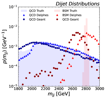
To emulate two different physics processes while controlling for all hidden variables, we consider dijet events with two different sets of event weights. This will allow us to study the prior-dependent effects of each calibration.
-
•
QCD. This set of weights comes from the original Pythia event generation. The resulting spectra are steeply falling in the invariant mass of the two jets, .
-
•
BSM. To emulate a narrow dijet resonance, we consider a second set of weights given by
(45) where TeV and GeV. Note that the weighting is applied using the true .
The distributions as described above are shown in Fig. 5. In the full simulation, one can see a difference between and for both QCD and BSM, necessitating a simulation-based calibration. Additionally, the distribution is significantly different between the full and fast simulations, which to correct requires a data-based calibration.
For all following results, half of the examples are used for training and half are used for testing.
V.2 Simulation-based Calibration
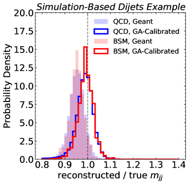
The goal for the simulation-based calibration is to learn a function to predict from in the full simulation. In contrast to the Gaussian example in Sec. IV.1, we do not know the functional form of the calibration. Therefore, we use a neural network to provide a flexible parametrization of the calibration and numerically minimize the MSE loss. The neural network has three hidden layers with 50 nodes per layer, with the rectified linear unit activation for intermediate layers and a linear activation for the output. The network is implemented in Keras with the Tensorflow backend and optimized with Adam using a batch size of 1000 and 50 epochs. Training is performed over the QCD sample to obtain the calibration function. The learned calibration function is then applied to both the QCD and BSM test samples.
The result of MSE calibration is shown in Fig. 6a. Prior to any calibration, the detector response is about 5% low in both the QCD and BSM test samples. After calibration, the mean is nearly unity for the QCD sample, albeit with a large width – that is to say, the average bias is close to zero over the prior, but the average resolution is large. For the BSM sample, though, the calibrated mean is far from unity, demonstrating the bias and prior dependence of the MSE calibration. The MSE-based calibration obtained from the QCD fit is not universal, and gives poor results when applied to the BSM sample.101010The converse is also true – attempting to use a calibration fitted on the BSM sample will lead to bias on the QCD sample, or any other BSM sample for that matter. These non-universal fits lead to mass sculpting, in which a fit depends strongly on the mass point used in training. See e.g. Kitouni et al. (2021) for discussions on sculpting and mass decorrelation.
For comparison, in Fig. 6b we show results from a maximum-likelihood-based calibration trained on the QCD sample, using the Gaussian Ansatz in Eq. (35). The , , , and networks of the Gaussian Ansatz each consist of three hidden layers with 32 nodes per layer, with the same activation functions, batch size, and epochs as in the Gaussian example. The calibration function trained on the QCD sample can be used for the BSM sample, and as Fig. 6b shows, the calibration is indeed universal and unbiased, as expected.
V.3 Data-based Calibration
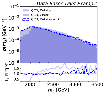
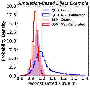
The goal for the data-based calibration task is to “correct” , given by the fast simulation (Delphes), to the observed data distribution , given by the full simulation (Geant4). We now apply the same procedure described in Sec. IV.2 to the dijet example.
An OT-based calibration is derived using QCD jets, to align the fast simulation Delphes) sample with the full simulation Geant4 sample. The calibration function, given by the optimal transport map (Eq. (17)), can be computed numerically by sorting and integrating the weighted data points to build the cumulative distribution functions. On the QCD sample, this calibration closes by construction. In particular, as shown in Fig. 7a, the blue dashed line in the ratio plot fluctuates around unity, with deviations due to statistical fluctuations that differ between the two halves of the event samples.
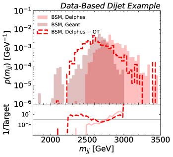
When this calibration is applied to the BSM events, however, the calibration overshoots, as shown with the red dashed line in the ratio plot in Fig. 7b. While the resulting dashed distribution agrees better with the data histogram in dark red than does the fast sim histogram in light red, the overall agreement is still rather poor. This again highlights the issue of prior dependence in data-based calibrations.
VI Conclusions
In this paper, we explored the prior dependence of machine-learning-based calibration techniques. There is a growing number of machine learning proposals for simulation-based and data-based calibration and in nearly all cases, there is a prior dependence. We highlighted the resulting calibration bias in a synthetic Gaussian example and a more realistic particle physics example of dijet production at the LHC.
In the simulation-based calibration case, most proposals learn a truth target from detector-level observables using loss functions like the MSE. A neural network trained in this way will learn the average true value given the detector-level inputs, which depends on the spectrum of truth values. However, we have shown that this will yield a calibration that lacks the critical properties of universality and closure.
There are fewer proposals for machine learning data-based calibrations, but we studied one recent idea based on OT and showed its prior dependence. While we focused on one-dimensional examples, the prior dependence is a generic feature of these approaches. Going to higher dimensions may even exacerbate the issue since it is harder to visualize and control prior differences in many dimensions.
New learning approaches are required to ensure that machine learning-based calibrations are universal. For simulation-based calibration, the ATLAS collaboration has proposed a prior-independent method called generalized numerical inversion ATLAS Collaboration (2018, 2020b). While prior independent, this technique is typically biased and does not scale well to many dimensions. We proposed a new approach based on maximum likelihood estimation in Ref. Gambhir et al. (2022), based on parametrizing the log-likelihood with a Gaussian Ansatz. Maximum-likelihood-based approaches are prior independent by construction and are well-motivated statistically. Parametrizing the maximum likelihood estimator with neural networks requires a different learning paradigm than current approaches, but it extends well to many dimensions. To our knowledge, there are currently no prior-independent data-based calibration approaches.
To make the most use of the complex data from the LHC and other HEP experiments, it is essential to use all of the available information for object calibration. This will require modern machine learning to account for all of the subtle correlations in high dimensions. It is important, however, that we construct these machine learning calibration functions in a way that integrates all of the features of classical calibration methods. We highlighted prior independence in this paper as a cornerstone of calibration. In the future, innovations that incorporate knowledge of the detector response or physics symmetries may further enhance the precision and accuracy of machine learning calibrations.
Code and Data
The code for this paper can be found at https://github.com/hep-lbdl/calibrationpriors, which makes use of Jupyter notebooks Kluyver et al. (2016) employing NumPy Harris et al. (2020) for data manipulation and Matplotlib Hunter (2007) to produce figures. All of the machine learning was performed on a Nvidia RTX6000 Graphical Processing Unit (GPU). The physics datasets are hosted on Zenodo at Refs. Komiske et al. (2019a, b, c); Nachman and Thaler (2021c).
Acknowledgements.
BN is supported by the U.S. Department of Energy (DOE), Office of Science under contract DE-AC02-05CH11231. RG and JT are supported by the National Science Foundation under Cooperative Agreement PHY-2019786 (The NSF AI Institute for Artificial Intelligence and Fundamental Interactions, http://iaifi.org/), and by the U.S. DOE Office of High Energy Physics under grant number DE-SC0012567.References
- Aad et al. (2017) Georges Aad et al. (ATLAS), “Topological cell clustering in the ATLAS calorimeters and its performance in LHC Run 1,” Eur. Phys. J. C 77, 490 (2017), arXiv:1603.02934 [hep-ex] .
- Sirunyan et al. (2017) A. M. Sirunyan et al. (CMS), “Particle-flow reconstruction and global event description with the CMS detector,” JINST 12, P10003 (2017), arXiv:1706.04965 [physics.ins-det] .
- Aad et al. (2021) Georges Aad et al. (ATLAS), “Jet energy scale and resolution measured in proton–proton collisions at TeV with the ATLAS detector,” Eur. Phys. J. C 81, 689 (2021), arXiv:2007.02645 [hep-ex] .
- Khachatryan et al. (2017) Vardan Khachatryan et al. (CMS), “Jet energy scale and resolution in the CMS experiment in pp collisions at 8 TeV,” JINST 12, P02014 (2017), arXiv:1607.03663 [hep-ex] .
- Aad et al. (2016) Georges Aad et al. (ATLAS), “Muon reconstruction performance of the ATLAS detector in proton–proton collision data at =13 TeV,” Eur. Phys. J. C 76, 292 (2016), arXiv:1603.05598 [hep-ex] .
- Sirunyan et al. (2020a) Albert M Sirunyan et al. (CMS), “Performance of the reconstruction and identification of high-momentum muons in proton-proton collisions at 13 TeV,” JINST 15, P02027 (2020a), arXiv:1912.03516 [physics.ins-det] .
- Aad et al. (2019a) Georges Aad et al. (ATLAS), “Electron and photon performance measurements with the ATLAS detector using the 2015–2017 LHC proton-proton collision data,” JINST 14, P12006 (2019a), arXiv:1908.00005 [hep-ex] .
- Khachatryan et al. (2015a) Vardan Khachatryan et al. (CMS), “Performance of Photon Reconstruction and Identification with the CMS Detector in Proton-Proton Collisions at sqrt(s) = 8 TeV,” JINST 10, P08010 (2015a), arXiv:1502.02702 [physics.ins-det] .
- Khachatryan et al. (2015b) Vardan Khachatryan et al. (CMS), “Performance of Electron Reconstruction and Selection with the CMS Detector in Proton-Proton Collisions at s = 8 TeV,” JINST 10, P06005 (2015b), arXiv:1502.02701 [physics.ins-det] .
- Aad et al. (2015) Georges Aad et al. (ATLAS), “Identification and energy calibration of hadronically decaying tau leptons with the ATLAS experiment in collisions at =8 TeV,” Eur. Phys. J. C 75, 303 (2015), arXiv:1412.7086 [hep-ex] .
- Sirunyan et al. (2018a) A. M. Sirunyan et al. (CMS), “Performance of reconstruction and identification of leptons decaying to hadrons and in pp collisions at 13 TeV,” JINST 13, P10005 (2018a), arXiv:1809.02816 [hep-ex] .
- Aad et al. (2019b) Georges Aad et al. (ATLAS), “ATLAS b-jet identification performance and efficiency measurement with events in pp collisions at TeV,” Eur. Phys. J. C 79, 970 (2019b), arXiv:1907.05120 [hep-ex] .
- Sirunyan et al. (2018b) A. M. Sirunyan et al. (CMS), “Identification of heavy-flavour jets with the CMS detector in pp collisions at 13 TeV,” JINST 13, P05011 (2018b), arXiv:1712.07158 [physics.ins-det] .
- Aaboud et al. (2019) Morad Aaboud et al. (ATLAS), “Performance of top-quark and -boson tagging with ATLAS in Run 2 of the LHC,” Eur. Phys. J. C 79, 375 (2019), arXiv:1808.07858 [hep-ex] .
- Sirunyan et al. (2020b) Albert M Sirunyan et al. (CMS), “Identification of heavy, energetic, hadronically decaying particles using machine-learning techniques,” JINST 15, P06005 (2020b), arXiv:2004.08262 [hep-ex] .
- Belayneh et al. (2020) Dawit Belayneh et al., “Calorimetry with deep learning: particle simulation and reconstruction for collider physics,” Eur. Phys. J. C 80, 688 (2020), arXiv:1912.06794 [physics.ins-det] .
- ATLAS Collaboration (2020a) ATLAS Collaboration, “Deep Learning for Pion Identification and Energy Calibration with the ATLAS Detector,” ATL-PHYS-PUB-2020-018 (2020a).
- Akchurin, N. and Cowden, C. and Damgov, J. and Hussain, A. and Kunori, S. (2021) Akchurin, N. and Cowden, C. and Damgov, J. and Hussain, A. and Kunori, S., “On the Use of Neural Networks for Energy Reconstruction in High-granularity Calorimeters,” (2021), arXiv:2107.10207 [physics.ins-det] .
- Akchurin et al. (2021) N. Akchurin, C. Cowden, J. Damgov, A. Hussain, and S. Kunori, “Perspectives on the Calibration of CNN Energy Reconstruction in Highly Granular Calorimeters,” (2021), arXiv:2108.10963 [physics.ins-det] .
- Polson et al. (2021) L. Polson, L. Kurchaninov, and M. Lefebvre, “Energy reconstruction in a liquid argon calorimeter cell using convolutional neural networks,” (2021), arXiv:2109.05124 [physics.ins-det] .
- Pata et al. (2021) Joosep Pata, Javier Duarte, Jean-Roch Vlimant, Maurizio Pierini, and Maria Spiropulu, “MLPF: Efficient machine-learned particle-flow reconstruction using graph neural networks,” (2021), arXiv:2101.08578 [physics.data-an] .
- Kieseler et al. (2021) Jan Kieseler, Giles C. Strong, Filippo Chiandotto, Tommaso Dorigo, and Lukas Layer, “Calorimetric Measurement of Multi-TeV Muons via Deep Regression,” (2021), arXiv:2107.02119 [physics.ins-det] .
- ATLAS Collaboration (2018) ATLAS Collaboration, “Generalized Numerical Inversion: A Neural Network Approach to Jet Calibration,” ATL-PHYS-PUB-2018-013 (2018).
- ATLAS Collaboration (2020b) ATLAS Collaboration, “Simultaneous Jet Energy and Mass Calibrations with Neural Networks,” ATL-PHYS-PUB-2020-001 (2020b).
- Sirunyan et al. (2020c) Albert M Sirunyan et al. (CMS), “A Deep Neural Network for Simultaneous Estimation of b Jet Energy and Resolution,” Comput. Softw. Big Sci. 4, 10 (2020c), arXiv:1912.06046 [hep-ex] .
- Haake and Loizides (2019) Rüdiger Haake and Constantin Loizides, “Machine Learning based jet momentum reconstruction in heavy-ion collisions,” Phys. Rev. C 99, 064904 (2019), arXiv:1810.06324 [nucl-ex] .
- Haake (2020) Rüdiger Haake (ALICE), “Machine Learning based jet momentum reconstruction in Pb-Pb collisions measured with the ALICE detector,” PoS EPS-HEP2019, 312 (2020), arXiv:1909.01639 [nucl-ex] .
- Baldi, Pierre and Blecher, Lukas and Butter, Anja and Collado, Julian and Howard, Jessica N. and Keilbach, Fabian and Plehn, Tilman and Kasieczka, Gregor and Whiteson, Daniel (2020) Baldi, Pierre and Blecher, Lukas and Butter, Anja and Collado, Julian and Howard, Jessica N. and Keilbach, Fabian and Plehn, Tilman and Kasieczka, Gregor and Whiteson, Daniel, “How to GAN Higher Jet Resolution,” (2020), arXiv:2012.11944 [hep-ph] .
- Komiske et al. (2017) Patrick T. Komiske, Eric M. Metodiev, Benjamin Nachman, and Matthew D. Schwartz, “Pileup Mitigation with Machine Learning (PUMML),” JHEP 12, 051 (2017), arXiv:1707.08600 [hep-ph] .
- ATL (2019) Convolutional Neural Networks with Event Images for Pileup Mitigation with the ATLAS Detector, Tech. Rep. (CERN, Geneva, 2019).
- Maier et al. (2022) B Maier, S M Narayanan, G de Castro, M Goncharov, Ch Paus, and M Schott, “Pile-up mitigation using attention,” Machine Learning: Science and Technology 3, 025012 (2022).
- Kasieczka et al. (2020a) Gregor Kasieczka, Michel Luchmann, Florian Otterpohl, and Tilman Plehn, “Per-Object Systematics using Deep-Learned Calibration,” (2020a), arXiv:2003.11099 [hep-ph] .
- Arjona Martínez et al. (2019) J. Arjona Martínez, Olmo Cerri, Maurizio Pierini, Maria Spiropulu, and Jean-Roch Vlimant, “Pileup mitigation at the Large Hadron Collider with graph neural networks,” Eur. Phys. J. Plus 134, 333 (2019), arXiv:1810.07988 [hep-ph] .
- Diefenthaler et al. (2021) Markus Diefenthaler, Abduhhal Farhat, Andrii Verbytskyi, and Yuesheng Xu, “Deeply Learning Deep Inelastic Scattering Kinematics,” (2021), arXiv:2108.11638 [hep-ph] .
- Liu et al. (2020) Junze Liu, Jordan Ott, Julian Collado, Benjamin Jargowsky, Wenjie Wu, Jianming Bian, and Pierre Baldi (DUNE), “Deep-Learning-Based Kinematic Reconstruction for DUNE,” (2020), arXiv:2012.06181 [physics.ins-det] .
- Delaquis et al. (2018) S. Delaquis et al. (EXO), “Deep Neural Networks for Energy and Position Reconstruction in EXO-200,” JINST 13, P08023 (2018), arXiv:1804.09641 [physics.ins-det] .
- Baldi et al. (2019) Pierre Baldi, Jianming Bian, Lars Hertel, and Lingge Li, “Improved Energy Reconstruction in NOvA with Regression Convolutional Neural Networks,” Phys. Rev. D 99, 012011 (2019), arXiv:1811.04557 [physics.ins-det] .
- Abbasi et al. (2021) R. Abbasi et al., “A Convolutional Neural Network based Cascade Reconstruction for the IceCube Neutrino Observatory,” JINST 16, P07041 (2021), arXiv:2101.11589 [hep-ex] .
- Aartsen et al. (2020) M. G. Aartsen et al. (IceCube), “Cosmic ray spectrum from 250 TeV to 10 PeV using IceTop,” Phys. Rev. D 102, 122001 (2020), arXiv:2006.05215 [astro-ph.HE] .
- Carloni et al. (2021) Kiara Carloni, Nicholas W. Kamp, Austin Schneider, and Janet M. Conrad, “Convolutional Neural Networks for Shower Energy Prediction in Liquid Argon Time Projection Chambers,” (2021), arXiv:2110.10766 [hep-ex] .
- Feickert and Nachman (2021) Matthew Feickert and Benjamin Nachman, “A Living Review of Machine Learning for Particle Physics,” (2021), arXiv:2102.02770 [hep-ph] .
- Pollard and Windischhofer (2021) Chris Pollard and Philipp Windischhofer, “Transport away your problems: Calibrating stochastic simulations with optimal transport,” (2021), arXiv:2107.08648 [physics.data-an] .
- Gambhir et al. (2022) Rikab Gambhir, Benjamin Nachman, and Jesse Thaler, “Learning uncertainties the frequentist way: Calibration and correlation in high energy physics,” (2022), arXiv:2205.03413 [hep-ph] .
- Cheong et al. (2020) Sanha Cheong, Aviv Cukierman, Benjamin Nachman, Murtaza Safdari, and Ariel Schwartzman, “Parametrizing the Detector Response with Neural Networks,” JINST 15, P01030 (2020), arXiv:1910.03773 [physics.data-an] .
- Cukierman and Nachman (2017) A. Cukierman and B. Nachman, “Mathematical Properties of Numerical Inversion for Jet Calibrations.” Nucl. Instrum. Meth. A 858, 1 (2017), arXiv:1609.05195 [physics.data-an] .
- Rezende and Mohamed (2015) Danilo Jimenez Rezende and Shakir Mohamed, “Variational inference with normalizing flows,” International Conference on Machine Learning 37, 1530 (2015).
- Kobyzev et al. (2020) Ivan Kobyzev, Simon Prince, and Marcus Brubaker, “Normalizing Flows: An Introduction and Review of Current Methods,” IEEE Transactions on Pattern Analysis and Machine Intelligence , 1 (2020).
- Nachman and Thaler (2021a) Benjamin Nachman and Jesse Thaler, “E Pluribus Unum Ex Machina: Learning from Many Collider Events at Once,” (2021a), arXiv:2101.07263 [physics.data-an] .
- Monroe D. Donsker and S. R. S. Varadhan (1975) Monroe D. Donsker and S. R. S. Varadhan, “Asymptotic evaluation of certain markov process expectations for large time,” Communications on Pure and Applied Mathematics 28, 1–47 (1975).
- Belghazi et al. (2018) Mohamed Ishmael Belghazi, Aristide Baratin, Sai Rajeswar, Sherjil Ozair, Yoshua Bengio, Aaron Courville, and R Devon Hjelm, “Mine: Mutual information neural estimation,” (2018), 10.48550/arxiv.1801.04062.
- Kullback and Leibler (1951) Solomon Kullback and Richard A Leibler, “On information and sufficiency,” The annals of mathematical statistics 22, 79–86 (1951).
- Guo et al. (2017) Chuan Guo, Geoff Pleiss, Yu Sun, and Kilian Q. Weinberger, “On calibration of modern neural networks,” in Proceedings of the 34th International Conference on Machine Learning, Proceedings of Machine Learning Research, Vol. 70, edited by Doina Precup and Yee Whye Teh (PMLR, 2017) pp. 1321–1330.
- Cranmer et al. (2015) Kyle Cranmer, Juan Pavez, and Gilles Louppe, “Approximating Likelihood Ratios with Calibrated Discriminative Classifiers,” (2015), arXiv:1506.02169 [stat.AP] .
- Rogozhnikov (2016) A. Rogozhnikov, “Reweighting with Boosted Decision Trees,” Proceedings, 17th International Workshop on Advanced Computing and Analysis Techniques in Physics Research (ACAT 2016): Valparaiso, Chile, January 18-22, 2016 762, 012036 (2016), arXiv:1608.05806 [physics.data-an] .
- Andreassen and Nachman (2020) Anders Andreassen and Benjamin Nachman, “Neural Networks for Full Phase-space Reweighting and Parameter Tuning,” Phys. Rev. D 101, 091901 (2020), arXiv:1907.08209 [hep-ph] .
- Diefenbacher et al. (2020) S. Diefenbacher, E. Eren, G. Kasieczka, A. Korol, B. Nachman, and D. Shih, “DCTRGAN: Improving the Precision of Generative Models with Reweighting,” Journal of Instrumentation 15, P11004 (2020), arXiv:2009.03796 [hep-ph] .
- Nachman and Thaler (2021b) Benjamin Nachman and Jesse Thaler, “Neural Conditional Reweighting,” (2021b), arXiv:2107.08979 [physics.data-an] .
- Louppe et al. (2017) Gilles Louppe, Michael Kagan, and Kyle Cranmer, “Learning to Pivot with Adversarial Networks,” in Advances in Neural Information Processing Systems, Vol. 30, edited by I. Guyon, U. V. Luxburg, S. Bengio, H. Wallach, R. Fergus, S. Vishwanathan, and R. Garnett (Curran Associates, Inc., 2017) arXiv:1611.01046 [stat.ME] .
- Dolen et al. (2016) James Dolen, Philip Harris, Simone Marzani, Salvatore Rappoccio, and Nhan Tran, “Thinking outside the ROCs: Designing Decorrelated Taggers (DDT) for jet substructure,” JHEP 05, 156 (2016), arXiv:1603.00027 [hep-ph] .
- Moult et al. (2018) Ian Moult, Benjamin Nachman, and Duff Neill, “Convolved Substructure: Analytically Decorrelating Jet Substructure Observables,” JHEP 05, 002 (2018), arXiv:1710.06859 [hep-ph] .
- Stevens and Williams (2013) Justin Stevens and Mike Williams, “uBoost: A boosting method for producing uniform selection efficiencies from multivariate classifiers,” JINST 8, P12013 (2013), arXiv:1305.7248 [nucl-ex] .
- Shimmin et al. (2017) Chase Shimmin, Peter Sadowski, Pierre Baldi, Edison Weik, Daniel Whiteson, Edward Goul, and Andreas Søgaard, “Decorrelated Jet Substructure Tagging using Adversarial Neural Networks,” (2017), arXiv:1703.03507 [hep-ex] .
- Bradshaw et al. (2019) Layne Bradshaw, Rashmish K. Mishra, Andrea Mitridate, and Bryan Ostdiek, “Mass Agnostic Jet Taggers,” (2019), arXiv:1908.08959 [hep-ph] .
- ATL (2018) “Performance of mass-decorrelated jet substructure observables for hadronic two-body decay tagging in ATLAS,” ATL-PHYS-PUB-2018-014 (2018).
- Kasieczka and Shih (2020) Gregor Kasieczka and David Shih, “DisCo Fever: Robust Networks Through Distance Correlation,” (2020), 10.1103/PhysRevLett.125.122001, arXiv:2001.05310 [hep-ph] .
- Xia (2019) Li-Gang Xia, “QBDT, a new boosting decision tree method with systematical uncertainties into training for High Energy Physics,” Nucl. Instrum. Meth. A930, 15–26 (2019), arXiv:1810.08387 [physics.data-an] .
- Englert et al. (2019) Christoph Englert, Peter Galler, Philip Harris, and Michael Spannowsky, “Machine Learning Uncertainties with Adversarial Neural Networks,” Eur. Phys. J. C79, 4 (2019), arXiv:1807.08763 [hep-ph] .
- Wunsch et al. (2019) Stefan Wunsch, Simon Jórger, Roger Wolf, and Gunter Quast, “Reducing the dependence of the neural network function to systematic uncertainties in the input space,” (2019), 10.1007/s41781-020-00037-9, arXiv:1907.11674 [physics.data-an] .
- Rogozhnikov et al. (2015) Alex Rogozhnikov, Aleksandar Bukva, V. V. Gligorov, Andrey Ustyuzhanin, and Mike Williams, “New approaches for boosting to uniformity,” JINST 10, T03002 (2015), arXiv:1410.4140 [hep-ex] .
- Collaboration (2020) CMS Collaboration, “A deep neural network to search for new long-lived particles decaying to jets,” Machine Learning: Science and Technology (2020), 10.1088/2632-2153/ab9023, 1912.12238 .
- Clavijo et al. (2020) Jose M. Clavijo, Paul Glaysher, and Judith M. Katzy, “Adversarial domain adaptation to reduce sample bias of a high energy physics classifier,” (2020), arXiv:2005.00568 [stat.ML] .
- Kasieczka et al. (2020b) Gregor Kasieczka, Benjamin Nachman, Matthew D. Schwartz, and David Shih, “ABCDisCo: Automating the ABCD Method with Machine Learning,” (2020b), 10.1103/PhysRevD.103.035021, arXiv:2007.14400 [hep-ph] .
- Kitouni et al. (2020) Ouail Kitouni, Benjamin Nachman, Constantin Weisser, and Mike Williams, “Enhancing searches for resonances with machine learning and moment decomposition,” (2020), arXiv:2010.09745 [hep-ph] .
- Ghosh and Nachman (2021) Aishik Ghosh and Benjamin Nachman, “A Cautionary Tale of Decorrelating Theory Uncertainties,” (2021), arXiv:2109.08159 [hep-ph] .
- Blance et al. (2019) Andrew Blance, Michael Spannowsky, and Philip Waite, “Adversarially-trained autoencoders for robust unsupervised new physics searches,” JHEP 10, 047 (2019), arXiv:1905.10384 [hep-ph] .
- Estrade et al. (2019) Victor Estrade, Cécile Germain, Isabelle Guyon, and David Rousseau, “Systematic aware learning - A case study in High Energy Physics,” EPJ Web Conf. 214, 06024 (2019).
- Wunsch et al. (2020) Stefan Wunsch, Simon Jörger, Roger Wolf, and Günter Quast, “Optimal statistical inference in the presence of systematic uncertainties using neural network optimization based on binned Poisson likelihoods with nuisance parameters,” (2020), 10.1007/s41781-020-00049-5, arXiv:2003.07186 [physics.data-an] .
- Elwood et al. (2020) A. Elwood, D. Krücker, and M. Shchedrolosiev, “Direct optimization of the discovery significance in machine learning for new physics searches in particle colliders,” J. Phys. Conf. Ser. 1525, 012110 (2020).
- De Castro and Dorigo (2019) Pablo De Castro and Tommaso Dorigo, “INFERNO: Inference-Aware Neural Optimisation,” Comput. Phys. Commun. 244, 170–179 (2019), arXiv:1806.04743 [stat.ML] .
- Charnock et al. (2018) Tom Charnock, Guilhem Lavaux, and Benjamin D. Wandelt, “Automatic physical inference with information maximizing neural networks,” Physical Review D 97 (2018), 10.1103/physrevd.97.083004.
- Alsing and Wandelt (2019) Justin Alsing and Benjamin Wandelt, “Nuisance hardened data compression for fast likelihood-free inference,” Mon. Not. Roy. Astron. Soc. 488, 5093–5103 (2019), arXiv:1903.01473 [astro-ph.CO] .
- Simpson and Heinrich (2022) Nathan Simpson and Lukas Heinrich, “neos: End-to-end-optimised summary statistics for high energy physics,” (2022), 10.48550/arXiv.2203.05570, arXiv:2203.05570 .
- Bollweg et al. (2020) Sven Bollweg, Manuel Haußmann, Gregor Kasieczka, Michel Luchmann, Tilman Plehn, and Jennifer Thompson, “Deep-Learning Jets with Uncertainties and More,” SciPost Phys. 8, 006 (2020), arXiv:1904.10004 [hep-ph] .
- Araz and Spannowsky (2021) Jack Y. Araz and Michael Spannowsky, “Combine and Conquer: Event Reconstruction with Bayesian Ensemble Neural Networks,” (2021), arXiv:2102.01078 [hep-ph] .
- Bellagente et al. (2021) Marco Bellagente, Manuel Haußmann, Michel Luchmann, and Tilman Plehn, “Understanding Event-Generation Networks via Uncertainties,” (2021), arXiv:2104.04543 [hep-ph] .
- Nachman (2019) Benjamin Nachman, “A guide for deploying Deep Learning in LHC searches: How to achieve optimality and account for uncertainty,” (2019), 10.21468/SciPostPhys.8.6.090, arXiv:1909.03081 [hep-ph] .
- Dorigo and de Castro (2020) Tommaso Dorigo and Pablo de Castro, “Dealing with Nuisance Parameters using Machine Learning in High Energy Physics: a Review,” (2020), arXiv:2007.09121 [stat.ML] .
- Ghosh et al. (2021) Aishik Ghosh, Benjamin Nachman, and Daniel Whiteson, “Uncertainty Aware Learning for High Energy Physics,” (2021), arXiv:2105.08742 [hep-ex] .
- Chollet (2017) Fraciois Chollet, “Keras,” GitHub repository (2017).
- Abadi et al. (2016) Martín Abadi, Paul Barham, Jianmin Chen, Zhifeng Chen, Andy Davis, Jeffrey Dean, Matthieu Devin, Sanjay Ghemawat, Geoffrey Irving, Michael Isard, et al., “Tensorflow: A system for large-scale machine learning.” in OSDI, Vol. 16 (2016) pp. 265–283.
- Kingma and Ba (2014) Diederik Kingma and Jimmy Ba, “Adam: A method for stochastic optimization,” (2014), arXiv:1412.6980 [cs] .
- Sjöstrand et al. (2006) Torbjorn Sjöstrand, Stephen Mrenna, and Peter Z. Skands, “PYTHIA 6.4 Physics and Manual,” JHEP 05, 026 (2006), arXiv:hep-ph/0603175 [hep-ph] .
- Chatrchyan et al. (2011) Serguei Chatrchyan et al. (CMS), “Measurement of the Underlying Event Activity at the LHC with TeV and Comparison with TeV,” JHEP 09, 109 (2011), arXiv:1107.0330 [hep-ex] .
- Agostinelli et al. (2003) S. Agostinelli et al. (GEANT4), “GEANT4–a simulation toolkit,” Nucl. Instrum. Meth. A 506, 250–303 (2003).
- Allison et al. (2006) J. Allison et al., “Geant4 developments and applications,” IEEE Transactions on Nuclear Science 53, 270–278 (2006).
- Allison et al. (2016) J. Allison et al., “Recent developments in Geant4,” Nucl. Instrum. Meth. A 835, 186–225 (2016).
- Chatrchyan et al. (2008) S. Chatrchyan et al. (CMS), “The CMS Experiment at the CERN LHC,” JINST 3, S08004 (2008).
- Sjöstrand et al. (2008) Torbjorn Sjöstrand, Stephen Mrenna, and Peter Z. Skands, “A Brief Introduction to PYTHIA 8.1,” Comput. Phys. Commun. 178, 852 (2008), arXiv:0710.3820 [hep-ph] .
- de Favereau et al. (2014) J. de Favereau, C. Delaere, P. Demin, A. Giammanco, V. Lemaître, A. Mertens, and M. Selvaggi (DELPHES 3), “DELPHES 3, A modular framework for fast simulation of a generic collider experiment,” JHEP 02, 057 (2014), arXiv:1307.6346 [hep-ex] .
- Mertens (2015) Alexandre Mertens, “New features in Delphes 3,” Proceedings, 16th International workshop on Advanced Computing and Analysis Techniques in physics (ACAT 14): Prague, Czech Republic, September 1-5, 2014, J. Phys. Conf. Ser. 608, 012045 (2015).
- Selvaggi (2014) Michele Selvaggi, “DELPHES 3: A modular framework for fast-simulation of generic collider experiments,” Proceedings, 15th International Workshop on Advanced Computing and Analysis Techniques in Physics Research (ACAT 2013): Beijing, China, May 16-21, 2013, J. Phys. Conf. Ser. 523, 012033 (2014).
- CMS Collaboration (2016a) CMS Collaboration, “Simulated dataset QCD_Pt-1000to1400_TuneZ2_7TeV_pythia6 in AODSIM format for 2011 collision data (SM Exclusive),” CERN Open Data Portal (2016a), 10.7483/OPENDATA.CMS.96U2.3YAH.
- CMS Collaboration (2016b) CMS Collaboration, “Simulated dataset QCD_Pt-1400to1800_TuneZ2_7TeV_pythia6 in AODSIM format for 2011 collision data (SM Exclusive),” CERN Open Data Portal (2016b), 10.7483/OPENDATA.CMS.RC9V.B5KX.
- CMS Collaboration (2016c) CMS Collaboration, “Simulated dataset QCD_Pt-1800_TuneZ2_7TeV_pythia6 in AODSIM format for 2011 collision data (SM Exclusive),” CERN Open Data Portal (2016c), 10.7483/OPENDATA.CMS.CX2X.J3KW.
- Komiske et al. (2020) Patrick T. Komiske, Radha Mastandrea, Eric M. Metodiev, Preksha Naik, and Jesse Thaler, “Exploring the Space of Jets with CMS Open Data,” Phys. Rev. D 101, 034009 (2020), arXiv:1908.08542 [hep-ph] .
- Komiske et al. (2019a) Patrick Komiske, Radha Mastandrea, Eric Metodiev, Preksha Naik, and Jesse Thaler, “CMS 2011A Simulation | Pythia 6 QCD 1000-1400 | pT > 375 GeV | MOD HDF5 Format,” (2019a).
- Komiske et al. (2019b) Patrick Komiske, Radha Mastandrea, Eric Metodiev, Preksha Naik, and Jesse Thaler, “CMS 2011A Simulation | Pythia 6 QCD 1400-1800 | pT > 375 GeV | MOD HDF5 Format,” (2019b).
- Komiske et al. (2019c) Patrick Komiske, Radha Mastandrea, Eric Metodiev, Preksha Naik, and Jesse Thaler, “CMS 2011A Simulation | Pythia 6 QCD1800-inf | pT > 375 GeV | MOD HDF5 Format,” (2019c).
- G. Kasieczka, B. Nachman, and D. Shih (2021) G. Kasieczka, B. Nachman, and D. Shih, “Neural Conditional Reweighting,” (2021), arXiv:2107.08979 [physics.data-an] .
- Nachman and Thaler (2021c) Benjamin Nachman and Jesse Thaler, “Delphes dijet dataset,” (2021c).
- Cacciari et al. (2012) Matteo Cacciari, Gavin P. Salam, and Gregory Soyez, “FastJet User Manual,” Eur. Phys. J. C72, 1896 (2012), arXiv:1111.6097 [hep-ph] .
- Cacciari and Salam (2006) Matteo Cacciari and Gavin P. Salam, “Dispelling the myth for the jet-finder,” Phys. Lett. B641, 57 (2006), arXiv:hep-ph/0512210 [hep-ph] .
- Cacciari et al. (2008) Matteo Cacciari, Gavin P. Salam, and Gregory Soyez, “The anti- jet clustering algorithm,” JHEP 04, 063 (2008), arXiv:0802.1189 [hep-ph] .
- Kitouni et al. (2021) Ouail Kitouni, Benjamin Nachman, Constantin Weisser, and Mike Williams, “Enhancing searches for resonances with machine learning and moment decomposition,” Journal of High Energy Physics 2021 (2021), 10.1007/jhep04(2021)070.
- Kluyver et al. (2016) Thomas Kluyver, Benjamin Ragan-Kelley, Fernando Pérez, Brian Granger, Matthias Bussonnier, Jonathan Frederic, Kyle Kelley, Jessica Hamrick, Jason Grout, Sylvain Corlay, Paul Ivanov, Damián Avila, Safia Abdalla, and Carol Willing, “Jupyter notebooks – a publishing format for reproducible computational workflows,” in Positioning and Power in Academic Publishing: Players, Agents and Agendas, edited by F. Loizides and B. Schmidt (IOS Press, 2016) pp. 87 – 90.
- Harris et al. (2020) Charles R. Harris, K. Jarrod Millman, St’efan J. van der Walt, Ralf Gommers, Pauli Virtanen, David Cournapeau, Eric Wieser, Julian Taylor, Sebastian Berg, Nathaniel J. Smith, Robert Kern, Matti Picus, Stephan Hoyer, Marten H. van Kerkwijk, Matthew Brett, Allan Haldane, Jaime Fern’andez del R’ıo, Mark Wiebe, Pearu Peterson, Pierre G’erard-Marchant, Kevin Sheppard, Tyler Reddy, Warren Weckesser, Hameer Abbasi, Christoph Gohlke, and Travis E. Oliphant, “Array programming with NumPy,” Nature 585, 357–362 (2020).
- Hunter (2007) J. D. Hunter, “Matplotlib: A 2d graphics environment,” Computing in Science & Engineering 9, 90–95 (2007).